The semi-annual oscillation (SAO) in the upper troposphere and lower stratosphere (UTLS)

Both the scientific and operational communities are increasingly interested in subseasonal to seasonal variations of weather and climate. The semi-annual oscillation (SAO) has been studied extensively at the surface as well as in the middle atmosphere (upper stratosphere and the lower mesosphere). However, the SAO in the upper troposphere and lower stratosphere (UTLS) has been less discussed. Here we find evident SAO of temperature in the UTLS (250–175 hPa) from the subtropics to middle latitudes (22.5–42.5^∘) using high-quality satellite measurements, reanalysis data, and model simulations. We show the mechanism of its formation by an energy budget analysis. The temperature in the Northern Hemisphere (NH) UTLS shows the first peak in February according to the dynamical heating and shows the second peak in July due to the dynamical heating and moist processes. Similar to the NH, the austral winter time maximum temperature in the Southern Hemisphere (SH) is related to dynamical heating and the austral summer time maximum is related to both moisture and dynamical heating in the UTLS. Model simulations indicate that the SAO in the UTLS is partly affected by the existence of an SAO in sea surface temperatures (SSTs) in the SH mid-latitudes and weakly affected by the SAO in SSTs in the NH mid-latitudes.

1 Introduction

Subseasonal to seasonal predictions of weather and climate are increasingly important due to the urgent requirements of decision makers (Merryfield et al., 2020). As an important component of subseasonal to seasonal variations, the semi-annual oscillation (SAO) has been well known at the surface (surface-SAO) (Meehl et al., 1998) as well as in the middle atmosphere (MA-SAO) (Garcia et al., 1997). It is well known that the annual cycle of temperature gradient and mean sea level pressure is dominated by a strong half-yearly oscillation between 50 and 65^∘ S, which exceeds the magnitude of the yearly wave in many locations in the SH near the surface (Walland and Simmonds, 1998; Simmonds and Jones, 1998). This surface-SAO is a coupled ocean-atmosphere phenomenon, and a change of the seasonal cycle of sea surface temperatures (SSTs) at 50^∘ S could alter the amplitude of the surface-SAO (Meehl et al., 1998). Bracegirdle (2011) showed that this surface SAO is coupled with the stratospheric circulation, and correlations are found over a large altitude range in the troposphere and stratosphere. Yang and Wu (2022) relate the semi-annual surface air response to changes in the oceanic mixed layers. The SAO is also noticeable as the dominating mode of wind and temperature variability in the tropical middle atmosphere between the middle stratosphere and the upper mesosphere (Read, 1962; Garcia et al., 1997). This MA-SAO is a complex interplay of momentum advection, planetary waves from the extratropics, and vertically propagating equatorial waves including both global-scale waves and small-scale gravity waves (Hamilton and Mahlman, 1988; Richter and Garcia, 2006; Ern et al., 2015, 2021).

In comparison, only a few studies focused on the SAO in the upper troposphere and lower stratosphere (UTLS). The SAO in temperature was reported by Loon (1967) over the middle troposphere in the SH with two maxima in March and September near the equinoxes, which is related to varying heating/cooling rates in different latitude bands. Loon and Jenne (1969) described the tropical-subtropical SAO of the zonal wind and temperature in the SH based on data of the 20 radiosonde stations in the upper troposphere (100–300 hPa). They also found that the amplitude of SAO in temperature and wind are different along different longitudes, i.e., with stronger signals in the Eastern Hemisphere (Loon and Jenne, 1969; Chen and Tsay, 2014). According to Loon and Jenne (1969), the temperature oscillation is the result of an intensification of vertical motions from autumn to winter and the zonal wind oscillation is associated with second harmonics of opposite phase in the temperature. Shea et al. (1995) made a further study on the tropical-subtropical SAO (TS-SAO) in the upper troposphere with more extensive data coverage. Shea et al. (1995) found that the TS-SAO of temperature, which has maxima in the transitional seasons in the tropics and peaks in the extreme seasons in the subtropics, resulted from a marked semi-annual variation of the winds in the tropics with maxima in the intermonsoon months. The precise mechanism for this oscillation seems somewhat unclear, but may be associated with thermal fluctuations connected with the movement of the intertropical convergence zone from one side of the Equator to the other and associated modulations of the mean meridional circulation (Read and Castrejón‐Pita, 2012).

While measurements in the UTLS are relatively sparse, reanalysis data are widely used to investigate temperature variabilities (Broeke, 2000; Fueglistaler et al., 2009; Gettelman et al., 2011; Wang et al., 2016; Shangguan et al., 2019). Despite the importance of the SAO in the mid-latitudes, there have been few articles focused on it since that of Loon (1967), and these have been mostly based on radiosonde and reanalysis data. With the development of satellite techniques, many new remote sensing data are available in the UTLS. According to many studies (Wickert et al., 2001, 2009; Ho et al., 2017), the Global Navigation Satellite System Radio Occultation (GNSS RO) can provide highly accurate temperature profiles from the middle-upper troposphere to lower stratosphere by measuring the time delay in occulted signals from one satellite to another. The first RO mission (Challenging Minisatellite Payload, CHAMP) was launched in 2001, and the Constellation Observing System for Meteorology, Ionosphere and Climate (COSMIC), which is a constellation of six satellites since late 2006 is widely applied in climate research (Ho et al., 2014; Randel and Wu, 2015; Gao et al., 2017). Compared with radiosonde data, the GNSS RO data have global coverage (both over continents and oceans) and are not affected by weather (Anthes et al., 2008).

In this study, we use the GNSS RO data and the latest ECMWF reanalysis ERA5 (Hersbach et al., 2019) and the NASA MERRA2 reanalysis (GMAO, 2015a, b) to study the SAO in the UTLS (UTLS-SAO), and to discuss its origin. We expand the oscillation using temperature data available from GNSS RO and reanalyses between 60^∘ N to 60^∘ S spanning the period 2001–2017, and using Hadley Centre SST data set (Rayner et al., 2003) for a spatial coherence picture in the same period. The latest ERA5 and MERRA2 data, which include more recent instrument observations and improved data assimilation methods, should provide more reliable estimates than earlier studies. Power spectrum densities (PSD) analysis is used to analyze the time scale of temporal variability and a significance test is used to diagnose whether the SAO signal is significant and not an artifact. In particular, the SAO investigated in this study is sinus-like with periods of ∼ 6 months, i.e., it is not just a harmonic of the annual cycle. The energy budget, i.e., the heating rates according to dynamical, radiative, and moist processes, are analyzed to explain the formation of the SAO in temperature. To understand the relationship between SAO and SSTs, three model simulations with NCAR’s Whole Atmosphere Community Climate Model, version 6 (WACCM6) are used. Details of the data and model simulations are described in Sect. 2. In Sect. 3, we show the analysis and results. Conclusions are summarized in Sect. 4.

2 Data and methods

2.1 GNSS RO temperature data

The CHAMP provides ca. 150 occultation events globally per day from May 2001 to October 2008, and COSMIC began providing 1000–3000 occultation events per day since late 2006 (Wickert et al., 2001; Anthes et al., 2008). Many studies have demonstrated that GNSS RO temperature data have good quality in the range 8–30 km (Schmidt et al., 2005, 2010; Ho et al., 2009, 2012). In our study, we make use of monthly mean temperature data at 500–10 hPa. About 100 observations per month per 5^∘ latitude grid can be provided by a single satellite CHAMP and more than 10 times the number of profiles are available since late 2006 due to the start of the COSMIC mission. WetPrf products are interpolated onto 100 m vertical resolution from 0.1 to 40 km based on the one-dimensional variational method (Kursinski et al., 2000; Wee and Kuo, 2015). According to Xu et al. (2017) biases could exist for altitudes below ∼ 5–8 km in the wetPrf. We use the reprocessed and post-processed RO data, which are stable and accurate observations for climate studies. The CHAMP wetPf2 version is 2016.2430 and the COSMIC-1 wetPrf products are 2013.3520 and 2016.1120.

The GNSS RO monthly zonal means of standard pressure level (400–10 hPa) were determined based on CHAMP and COSMIC-1 for the period 2001–2017, for this, 5^∘ nonoverlapping latitude bands centered at 57.5^∘ S–57.5^∘ N were used. Data exceeding 3 times the standard deviation have been discarded at each level. For the COSMIC-1 data, we make additional monthly zonal means of standard pressure levels with a grid resolution 10^∘ (latitude) × 10^∘ (longitude) for the period 2007–2017. The same averaging strategy is used.

The GNSS RO data are available from May 2001 with some missing data during August–September 2001 and January–February 2002. Due to the missing data in the early part of the GNSS RO records, a spectral analysis of temperature data was performed using a Lomb-Scargle periodogram to identify the various periods in the time series (Lomb, 1976; Scargle, 1982; Horne and Baliunas, 1986; Press and Rybicki, 1989). The Lomb-Scargle periodogram can handle the periodic signals with missing data. For the SAO we choose the maximum PSD between 5 and 7 months and use the probability 0.95 of detection for the significance test (Horne and Baliunas, 1986). The significance test is used to check whether the peak is a true signal peak and not the result of random fluctuations.

2.2 Reanalysis data

The ERA5 is the latest ECMWF reanalysis (released in 2018) and various newly reprocessed data sets, recent instruments, improved data assimilation system are used in ERA5 (Hersbach et al., 2020). Detailed information can be found in ERA5 data documentation https://confluence.ecmwf.int/display/CKB/ERA5:+data+documentation (last access: 18 July 2022). The ERA5 monthly averaged data on pressure levels from 2001 to 2017 with 2.5^∘ horizontal resolution are downloaded from Climate Data Store (CDS) (Hersbach et al., 2019). MERRA2 is the latest atmospheric reanalysis of NASA's Global Modeling and Assimilation Office (GMAO) with data resolution 0.5^∘ × 0.625^∘ (Gelaro et al., 2017). Both reanalyses contain the eastward wind (u), northward wind (v), vertical pressure velocity (ω) and temperature (T) on pressure levels. Both reanalyses have assimilated GNSS RO bending angles.

2.3 Model simulations

The WACCM6 is one of the two available atmospheric components of the Community Earth System Model (CESM) from NCAR. It simulates atmospheric processes from the surface to about 140 km, which resolves the stratospheric dynamical and chemical processes well (Marsh et al., 2013; Gettelman et al., 2019). The standard version of WACCM has 70 vertical levels with a vertical resolution of about 1 km in the UTLS region (Gettelman et al., 2019; Wang et al., 2019). The horizontal resolution used here is 1.9^∘ × 2.5^∘.

The model is integrated into its atmosphere-only mode, with prescribed SSTs. We first employ a control simulation, with SSTs prescribed to historically observed values over the period from 2001 to 2017. The SSTs are provided by the Hadley Centre SST data set (Rayner et al., 2003). For comparison, we then employ two sensitivity simulations, which removed the SAO of SSTs (SST-SAO) globally (rmSAO run) and in the Tropics (rmSAO-TP run). The SST-SAO is removed by a band-pass filter (signals between 5 and 7 months are removed) using the Butterworth method (Butterworth, 1930). The differences between these two sensitivity simulations and the control simulation, therefore, indicate the influences of the SST-SAO on the UTLS-SAO.

2.4 Thermal budget analysis

To explain the SAO of temperature in the UTLS, the thermal budget is analyzed using the MERRA2 reanalysis as well as model simulations. The thermal budget of the UTLS is a balance between the dynamical heating and the total diabatic (Gettelman and Birner, 2007). The thermodynamic balance formalism is expressed as (Andrews et al., 1987; Abalos et al., 2013):

$$\begin{array}{}\text{(1)}& {\displaystyle }\stackrel{\mathrm{‾}}{T_t}=-{\stackrel{\mathrm{‾}}{v}}^{*}\stackrel{\mathrm{‾}}{T_y}-{\stackrel{\mathrm{‾}}{w}}^{*}S-e^{\frac{z}{H}}\left[e^{\frac{-z}{H}}\right(\stackrel{\mathrm{‾}}{v^{\prime }{t}^{\prime }}{\displaystyle \frac{\stackrel{\mathrm{‾}}{T_y}}{S}}+\stackrel{\mathrm{‾}}{w^{\prime }{T}^{\prime }}){]}_z+\stackrel{\mathrm{‾}}{Q}\text{(2)}& {\displaystyle }{\stackrel{\mathrm{‾}}{v}}^{*}=\stackrel{\mathrm{‾}}{v}-{\mathit{\rho }}_{\mathrm{0}}^{-\mathrm{1}}[{\mathit{\rho }}_{\mathrm{0}}\stackrel{\mathrm{‾}}{v^{\prime }{\mathrm{\Theta }}^{\prime }}/{\stackrel{\mathrm{‾}}{\mathrm{\Theta }}}_z{]}_z\text{(3)}& {\displaystyle }{\stackrel{\mathrm{‾}}{w}}^{*}=\stackrel{\mathrm{‾}}{w}+\left(a\cos \mathit{\varphi }{)}^{-\mathrm{1}}\right[\cos \mathit{\varphi }\stackrel{\mathrm{‾}}{v^{\prime }{\mathrm{\Theta }}^{\prime }}/{\stackrel{\mathrm{‾}}{\mathrm{\Theta }}}_z{]}_{\mathit{\varphi }},\end{array}$$

where H is 7 km, ρ₀ is the atmosphere density, ϕ is latitude, overbars in the equation denote zonal means, primes indicate deviations from it and subscripts denote partial derivatives. ${\stackrel{\mathrm{‾}}{v}}^{*}$ and ${\stackrel{\mathrm{‾}}{w}}^{*}$ are components of the residual circulations, which can be calculated by Eqs. (2)–(3). $\stackrel{\mathrm{‾}}{w}$ is the zonal mean vertical velocity, which is converted from the vertical pressure velocity ω in the reanalysis. Θ denotes potential temperature. $S=H\frac{N^{\mathrm{2}}}{R}$ with R=287 m² s⁻² K⁻¹ and N² is the Brunt-Väisälä frequency. The first three terms on the right side of the Eq. (1) indicate the dynamical heating, while Q is the diabatic heating. The dynamical heating includes the heating by the meridional component of the residual circulation (the first term on the right side of Eq. (1), the heating/cooling by downwelling/upwelling (the second term on the right side of Eq. (1), and heating related to eddys (the third term on the right side of Eq. (1), mainly associated with the vertical eddy heat flux). In the UTLS region, Q is mainly determined by radiation and moisture condensation processes.

The MERRA2 provides very detailed temperature tendencies related to dynamics, radiation, moisture, friction, gravity wave drag and near-surface turbulence. In the UTLS region, the friction, gravity wave drag and near-surface turbulence terms are very small, then we only use the dynamics, radiation and moisture terms in this study. In addition, to keep a balance of the thermal budget during the data assimilation, an extra term called the analysis tendencies (ANA) is used in MERRA2 reanalysis (Mapes and Bacmeister, 2012). ANA can be interpreted as the negative of model physical tendency error. Therefore, the ANA can be considered as residual (Mapes and Bacmeister, 2012). We further calculate the first two terms in Eq. (1) with the given equations and then separate the dynamical term of MERRA2 into the meridional component of the residual circulation, the heating by downwelling and eddy terms.

In the WACCM6 model, the temperature tendencies related to dynamics, radiation, moisture and gravity wave drag processes are also diagnosed and have direct outputs (Gettelman and Birner, 2007). Here we also use the dynamics, radiation and moisture terms in this study. The radiation term consists of long-wave and short-wave terms in the simulation. The dynamical term is also separated into the meridional component of the residual circulation, the heating by downwelling and eddy terms with the same method as MERRA2.

3 Analysis and results

3.1 Spatial distribution of the SAO

According to the Lomb-Scargle PSD values for the temperature data, the annual cycle is strongest in most of the regions. Figure 1 shows the SAO PSD in the period 2001–2017 and the lapse rate tropopause determined from GNSS RO data. The most prominent SAO signal with strong and significant SAO PSD can be seen in the UTLS region (250–175 hPa) from the subtropics (22.5^∘) to mid-latitudes (42.5^∘) in both hemispheres. This is also observed in the ratio of semi-annual/annual cycle PSD (Fig. S1 in the Supplement). The ratio is larger than 0.6 in the UTLS (300–175 hPa) from the subtropics to mid-latitudes (20–45^∘) and middle-upper troposphere (500–200 hPa) from tropics (10^∘ S–10^∘ N). The most prominent SAO PSDs can also be seen in the tropics from 400 to 225 hPa (Figs. 1 and S1). This is consistent with the results from Loon and Jenne (1969), which shows clear SAO of temperature in the upper troposphere in the tropics and SH subtropics. Our results give a survey of the SAO and find that the significant SAO also persists in the lower stratosphere and the mid-latitudes, i.e., 70–30 hPa in SH (32.5–47.5^∘ S) and NH (37.5–47.5^∘ N) mid-latitudes. It is also noteworthy that the magnitude of SAO PSD in the tropics in the troposphere and lower stratosphere is much weaker than the signals in mid-latitudes. In consideration of the peak of SAO PSD magnitude, we then mainly focus on the SAO in the UTLS region (250–175 hPa) in mid-latitudes (32.5–42.5^∘) hereafter in this study.

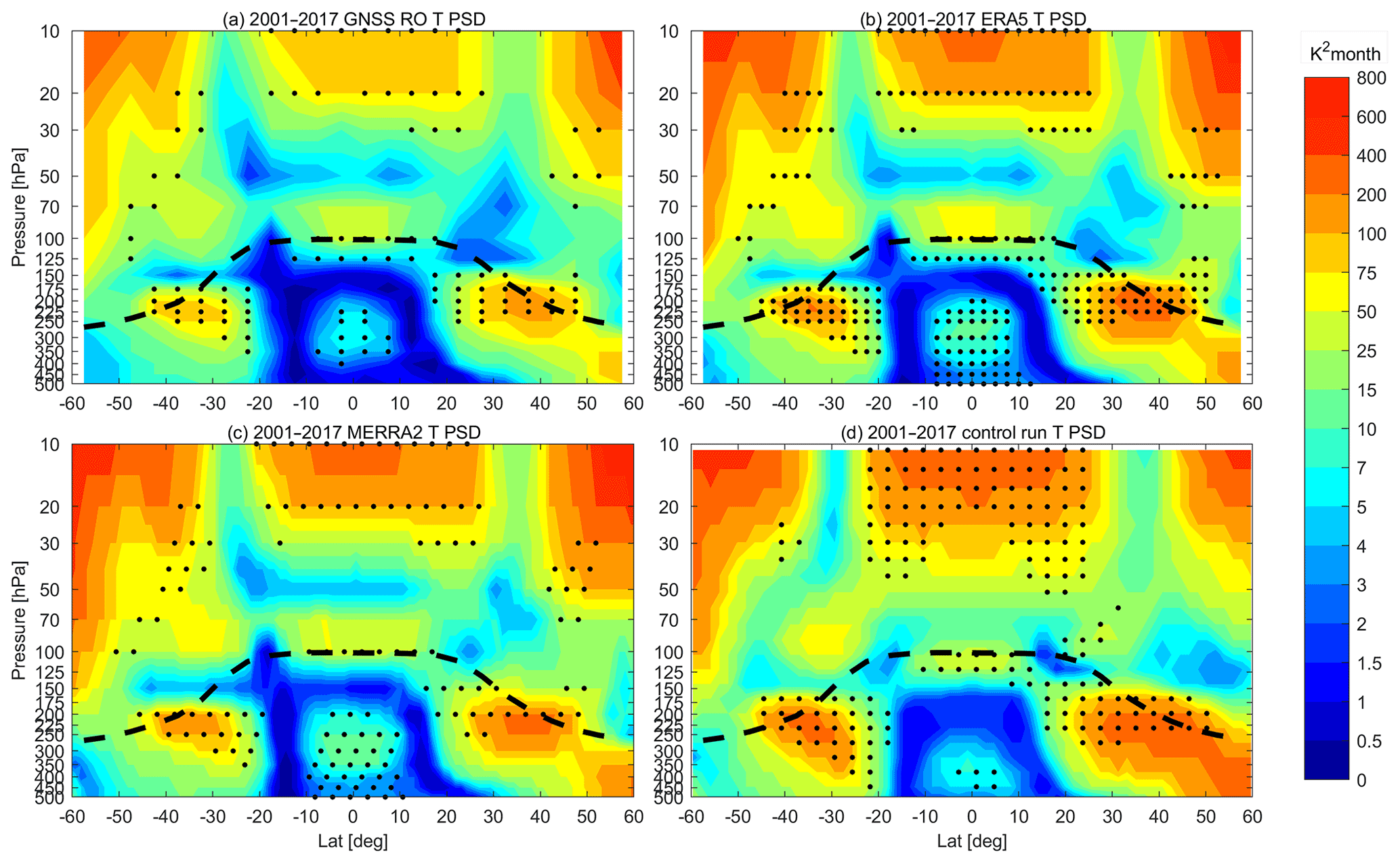
Figure 1 The power spectrum densities (PSD) of SAO based on GNSS RO (a), ERA5 (b), MERRA2 (c) and model simulation (d) temperature for the period 2001–2017. The dots mark the significant area at 95 % level. The dashed black lines mark the tropopause height calculated with GNSS RO data.

The reanalysis data and model simulations show good agreement with GNSS RO for the general pattern of SAO PSD. The ERA5 data show the best agreement with the GNSS RO, with a very similar spatial pattern and comparable magnitude as shown in Fig. 1a–b. The SAO signals in MERRA2 are slightly weaker and less significant than those in GNSS RO and ERA5 (Figs. 1c and S1c). The model also shows a good representation of the SAO in the UTLS, except that the significant region of SAO in the tropical regions is not observed from 350 to 200 hPa (Figs. 1d and S1d).

Further information can be gained from Fig. 2, which shows the latitude-longitude distributions of the SAO PSD at 200 hPa. The significant SAO region at 200 hPa in mid-latitudes is larger in the Eastern than in the Western Hemisphere, which is consistent with previous studies (Loon and Jenne, 1969). Note that due to data limitation of the CHAMP (ca. 150 occultation events globally per day), the PSD shown in Fig. 2a is calculated for the period 2007–2017. Further analysis indicates that the different period of analysis does not influence the results. As shown in Fig. S2, the PSD distribution 2007–2017 from the ERA5, MERRA2 and the control simulation is very similar to that shown in Fig. 2, which is analyzed for the period 2001–2017. Large SAO PSD occurs around the Asian region (25–45^∘ N, 20–100^∘ E), the Australian region (45–30^∘ S, 30–180^∘ E), as well as the North American region around the Great Lakes. The strong SAO signals over that region are likely related to both moist and dynamical processes. As seen in Figs. S3 and S4, there are strong upward motion over South Asia but downward motion from North Africa to Central Asia. The strong upwelling brings a large amount of water vapor from the surface to the upper troposphere, which condenses there and heats the atmosphere at around 200 hPa. At the same time, the strong downwelling leads to dynamical heating over the regions from North Africa to Central Asia. A further energy budget analysis indicates that the vertical transportation of water vapor and subsequent condensation in the upper troposphere over the Asian region is much stronger than in other regions and leads to a stronger peak of temperature in the summer season (Fig. S5). In addition, the radiative cooling is relatively weaker than in other regions, which also contributes to the stronger temperature peak in the Asia region (Fig. S5). Again, the ERA5 has the best agreement with GNSS RO measurements with a consistent pattern and comparable magnitude (Fig. 2b). The MERRA2 and the model simulation also show good agreement with the GNSS RO data (Fig. 2c–d). It is noteworthy that there are also significant SAO signals in the Tropics except over the Pacific. However, the magnitude of the SAO PSD in the Tropics is much weaker than that in mid-latitudes. According to previous studies, the SAO of the tropical stationary eddies is caused by the semi-annual east-west seesaw of the global divergent circulation between the areas of the Asian-Australian (AA) monsoon (60^∘ E–120^∘ W) and the extra-AA monsoon (120^∘ W–60^∘ E) particularly in SH tropics (Chen and Wu, 1992; Chen et al., 1996).

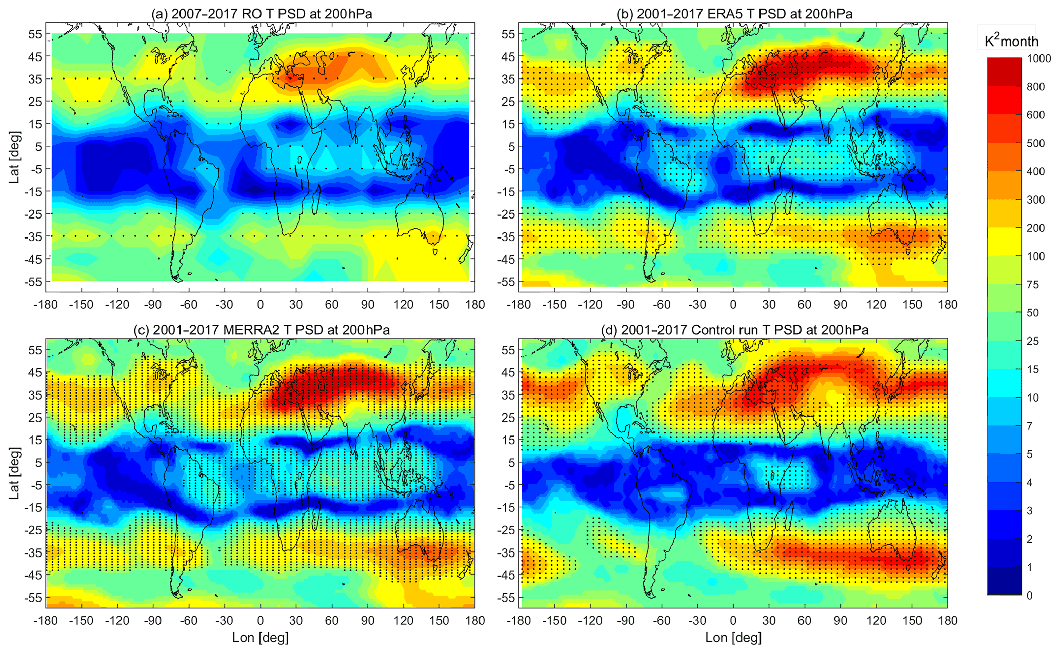
Figure 2 The PSD of SAO based on COSMIC-1 (2007–2017) (a), ERA5 (2001–2017) (b), MERRA2 (2001–2017) (c) and model simulation (2001–2017) (d) at 200 hPa. The dots mark the significant area at 95 % level.

3.2 Time evolution and mechanism of the SAO in the UTLS

To analyze the time evolution of SAO signals, Fig. 3 shows the time series in the zonal mean temperature and corresponding annual cycle anomalies in the NH mid-latitudes (NHM) (32.5–42.5^∘ N) and SH mid-latitudes (SHM) (32.5–42.5^∘ S) at 200 hPa. From the time series, the SAO of temperature is evident in both hemispheres, with two clear peaks of temperature in each year. Such oscillation can be seen in all the observed and reanalysis data sets, including the GNSS RO measurements as well as the ERA5 and MERRA2 reanalysis. The model simulations can also simulate the SAO of temperature except that there is an offset of about 1 K between the control simulation and the observation or reanalysis. From the annual cycle anomalies, two peaks of temperature exist in February and July in the NHM and in February and August in the SHM. The peak in July/August is more intense than in February, especially in the NHM. For all the datasets, the peaks in January–February and July–August are relatively even in NHM. In SHM the peak of simulations in August is weaker than observation/reanalysis.

Figure 3 Time series of the zonal mean temperature (T) at 200 hPa averaged around the Northern Hemisphere mid-latitudes (NHM) 32.5–42.5^∘ N (a) and their corresponding annual cycle anomalies (b). The Southern Hemisphere mid-latitudes (SHM) 32.5–42.5^∘ S (c) and their corresponding annual cycle anomalies (d).

To further investigate the mechanism of the SAO in the UTLS, the thermal budget is analyzed using the MERRA2 data and model simulations. The annual cycle of the heating rates at 200 hPa averaged over the latitude bands from 32.5 to 42.5^∘ in the two hemispheres is shown in Fig. 4. To show the relationship between the heating rates and the temperature, the annual cycle of temperature from the MERRA2 reanalysis data is also shown in Fig. 4. In the NHM, there are two peaks of total heating rates in December and June and two nadirs in March and September (Fig. 4a). While the total heating rate is positive, the temperature will increase. The total heating rates are positive from mid-November to mid-January and from April to July, which leads to increases in temperature during the same periods. From mid-January and July, the total heating rate turns to be negative, and the temperature starts to decrease. Therefore, there are two peaks of temperature in February and July. At the same time, there are two nadirs of temperature in April and November. To clearly show the relative contribution of different terms to the total heating rate, the variation of each term at peaks and nadirs of total heating rates is selected and shown in Fig. 5a. Overall, the dynamical processes contribute the most prominent positive heating rates through all terms, which is mostly offset by the radiative cooling. The radiative term can further be separated into short-wave warming and long-wave cooling (Fig. S6a). The short-wave and long-wave terms are all strongest during summer and the radiative heating rates are negative due to larger negative value of long-wave terms. The moisture and analysis terms are quite small. For the first temperature peak in January–February, it is mainly related to the dynamical heating, since the dynamical warming is slightly stronger than the radiative cooling and other terms are near zero in December. The second temperature peak in July is caused by a combination of moist and dynamical processes. There is a secondary peak of dynamical heating in June, although it is offset by radiative cooling. The moist processes delay the transition of total heating rates from positive to negative, which is in July but would be 1 month earlier otherwise. This positive peak in moist heating is related to the release of heat by the condensation of water vapor that is transported by deep convections in the upper troposphere. The negative total heating rates in March and September are mainly determined by the strong radiative cooling, which is stronger than the sum of the other terms.

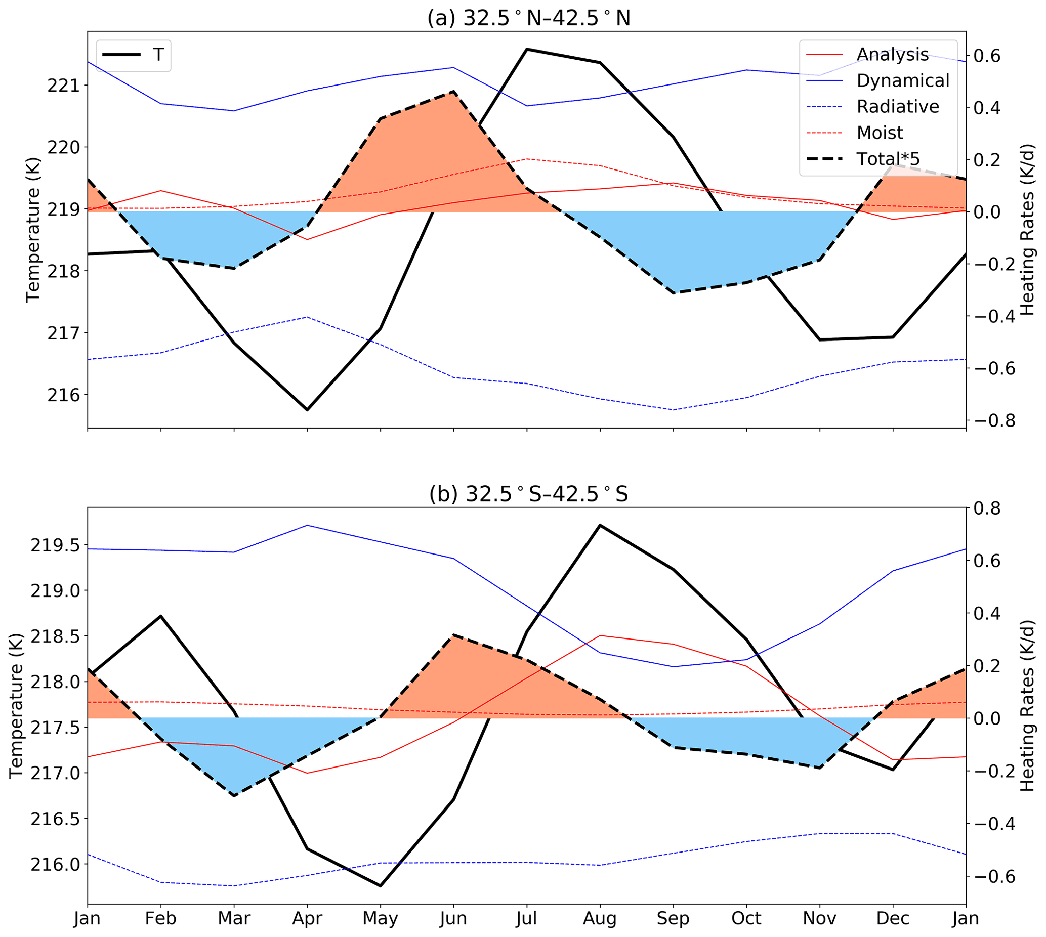
Figure 4 Annual cycle of the zonal mean temperature (T) and heating rates at 200 hPa averaged around the NHM 32.5–42.5^∘ N (a) and the SHM 32.5–42.5^∘ S (b) based on MERRA2 data. The red, blue, dashed blue and dashed red lines indicate the heating rates related to analysis tendency dynamics, radiation and condensation, respectively. The positive total heating rates are filled with light red color and the negative total heating rates are filled with light blue color. The total heating rates, which are the sum of analysis, dynamical, radiative and moist heating rates, have been enlarged 5 times to be more visible in the figures.

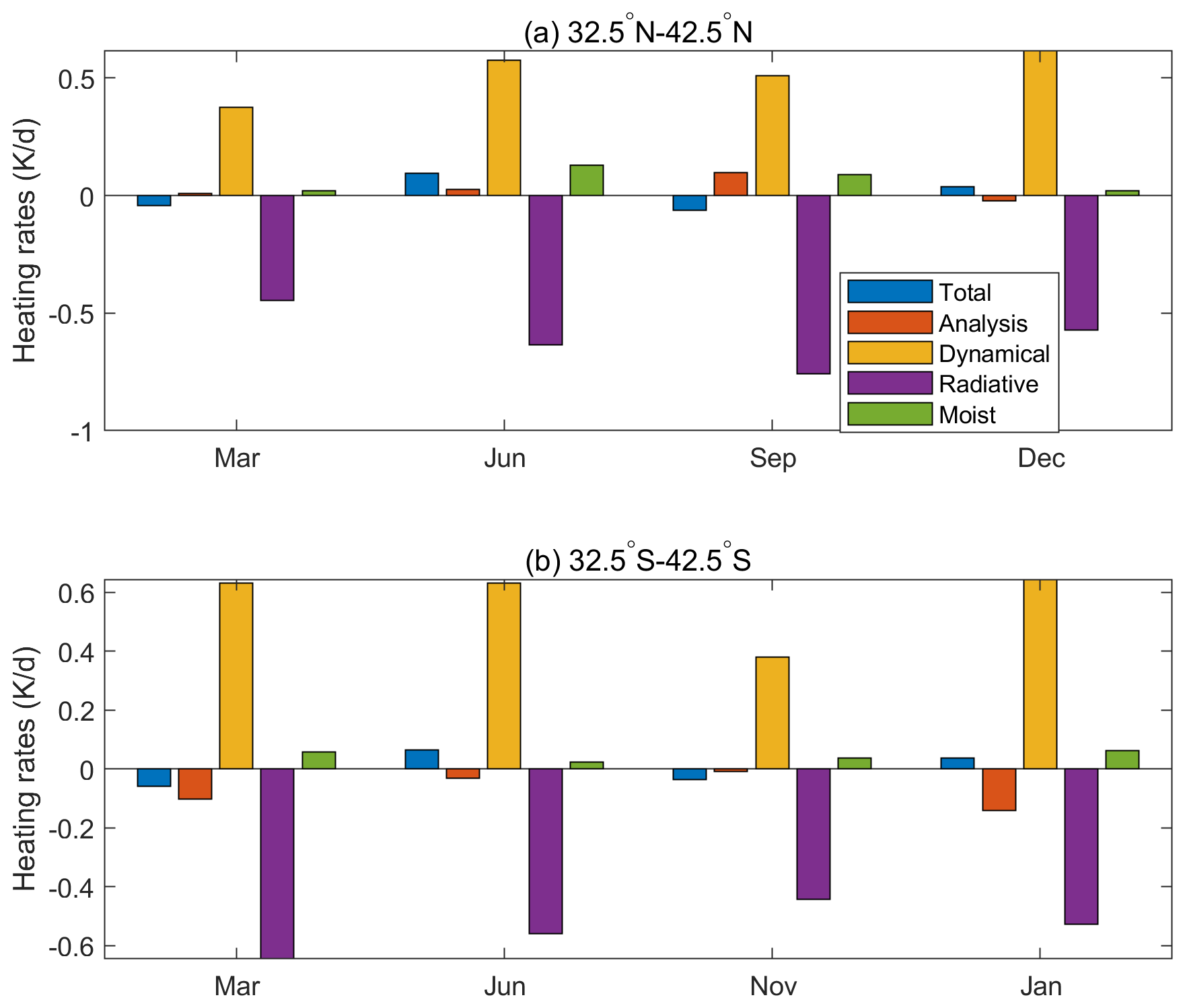
Figure 5 The variation of heating rates terms at 200 hPa at peaks and troughs of the total heating rates around the NHM 32.5–42.5^∘ N (a) and the SHM 32.5–42.5^∘ S (b) based on MERRA2 data. The blue, red, yellow, purple and green bars are total, analysis tendency, dynamical, radiative and moisture terms, respectively.

In the SHM (Figs. 4b and 5b), the total heating rates are positive from mid-November to mid-January and from May to August, which leads to a first peak of temperature in February and the second peak in August. For the SH austral summer, although the annual variation of the moist heating is relatively weak, it is stronger in DJF than in other months. In addition, the dynamical heating is also relatively strong in DJF. Therefore, both the dynamical and moist processes contribute to the positive total heating rates and lead to the temperature peak in SH austral summer. For the SH austral winter, the positive total heating rate and subsequent temperature maximum are mainly related to dynamical heating. Note that the ANA term in the SHM is large, which indicates a poor ability of the MERRA2 model to represent the temperature variations in SHM UTLS. The moist processes are lower in the SHM than in the NHM, which is perhaps due to overall weaker monsoon circulation. The energy budget analysis can also be confirmed by model simulations (Fig. S7). Figure S7 is the same as Fig. 4 but for the control simulation. The model shows a very similar annual variation of dynamical, radiative, moisture and total heating rates in both the NHM and SHM compared to the MERRA2 reanalysis.

In Fig. 6 the dynamical term is further divided into the eddy, heating by downwelling (−wS) and heating by the meridional component of the residual circulation (−vT_y) terms according to Eq. (1). The eddy term is mainly associated with the vertical eddy heat flux. As seen from Fig. 6, the −vT_y term is close to zero, which is less important in the UTLS region than other terms as also indicated by previous studies (Abalos et al., 2013). The −wS term is strongest during boreal winter (DJF) in both hemispheres, since the vertical component of the residual circulation (including the tropical upwelling and the extratropical downwelling) is most prominent in DJF. This is consistent with previous studies which shows a strongest dynamical cooling according to the upwelling in the Tropics (Abalos et al., 2013). In the SH, there is a secondary peak of the −wS term in JJA. The eddy term is non-negligible in the upper troposphere (at 200 hPa) and peaks from April to June. The first peak in dynamical heating during boreal winter (DJF) is dominated by the −wS term while the secondary peak near June is significantly influenced by the eddy term.

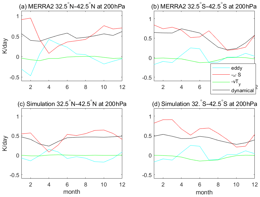
Figure 6 Annual cycle of dynamical heating rates at 200 hPa averaged around the NHM 32.5–42.5^∘ N (a) and the SHM 32.5–42.5^∘ S based on MERRA2 (a–b) and control simulation (c–d). The cyan, red, green and black lines are the eddy, heating by downwelling (−wS), heating by the meridional component of the residual circulation (−vT_y) and dynamical term, respectively.

3.3 Relationship between the UTLS-SAO and the SSTs

As introduced in Sect. 1, there is also a pronounced SAO signal at the surface (Meehl et al., 1998). While the surface is the main energy source of the atmosphere, it would be very interesting to investigate the relationship between the UTLS-SAO and the surface-SAO. Since the surface-SAO is a coupled ocean-atmosphere phenomenon and is strongly modified by the seasonal cycle of SSTs (Meehl et al., 1998), we mainly focus on the relationship between the UTLS-SAO and the SAO in SSTs (SST-SAO) in this study. We checked the PSD of the SST-SAO (Fig. S8), and there are significant SAO signals in the Tropics from the Eastern Pacific (120^∘ W) to the Atlantic Ocean, Indian Ocean and the Western Pacific (150^∘ E), which was also found by earlier studies (Schott et al., 2009; Park and Lee, 2014; Yan et al., 2018). The SST-SAO in the Pacific and Atlantic oceans in the Tropics is related to the SAO of solar radiation (Yashayaev and Zveryaev, 2001), while the SST-SAO in the tropical Indian Ocean is related to the Indian monsoon (Hu et al., 2005). The SAO signals over the Central Pacific (150^∘ E–120^∘ W) are not significant (Fig. S8), which resembles the UTLS-SAO in the tropics as shown in Fig. 2. This indicates the potential connection between the SST-SAO and the UTLS-SAO in the Tropics.

To identify the relationship between the subtropical to mid-latitude UTLS-SAO and the SST-SAO, the correlation coefficients are calculated between the SST-SAO and ULTS SAO in the tropical (5^∘ S–5^∘ N) and the SH/NH mid-latitude (Fig. S9). Firstly, we extracted ERA5 temperature SAO signals (5–7 months) using the 1-D wavelet Morlet transform (Lilly and Olhede, 2009, 2012). Secondly, we calculated the Pearson correlation coefficient between SAO signals and SST-SAOs. As shown in Fig. S9, both the SH/NH mid-latitude and tropical UTLS-SAO are strongly and significantly correlated with SST variations. The UTLS-SAO shows a positive correlation with SST-SAO in the tropics (5^∘ S–5^∘ N), especially over the Indian Ocean and the Western Pacific (Fig. S9c), whereas the SST-SAO is most pronounced (Fig. S8). The SH/NH mid-latitudes show very similar correlation patterns with SST-SAO (Fig. S9a–b) since the UTLS-SAO in the two hemispheres are almost in phase with each other (Fig. 3). All correlations are mainly negative in Fig. S9a–b, which indicate there are global phase variations.

We then further investigate the impacts of the SST-SAO on UTLS-SAO using our model simulations. As introduced in Sect. 2.3, we first employ a control simulation using the WACCM6 model with SSTs prescribed to observed variations. As seen in Figs. 1–3, the model represents the UTLS-SAO relatively well although the simulated temperature is ca. 1 K lower than observations. We then employ a sensitive simulation with the same configuration except that the SST-SAO has been removed globally (the rmSAO run). As discussed above, SST-SAO is mainly significant in the Tropics (Fig. S8), and the UTLS-SAO is most correlated with tropical SSTs, therefore we employ a third simulation with the SST-SAO removed only in the Tropics (the rmSAO-TP simulation).

Figure 7 shows the PSD of SAO in temperature from the rmSAO and rmSAO-TP runs, as well as their relative differences with respect to the control simulation. Similar to the control simulation, there are significant SAO signals in the rmSAO and rmSAO-TP simulations. When the SST-SAO is removed globally, the SAO in the tropical upper–middle troposphere (500–175 hPa) is not significant. However, if the SST-SAO is removed only in the Tropics, the upper troposphere SAO in the Tropics is still significant, which indicates that the upper–middle troposphere SAO in the Tropics is significantly influenced by the SST-SAO in the extratropics. At the same time, the SAO in the lower stratosphere of mid-latitudes (70–30 hPa in SH 32.5–47.5^∘ S and NH 37.5–47.5^∘ N) is also significantly reduced in both the rmSAO and rmSAO-TP simulations.

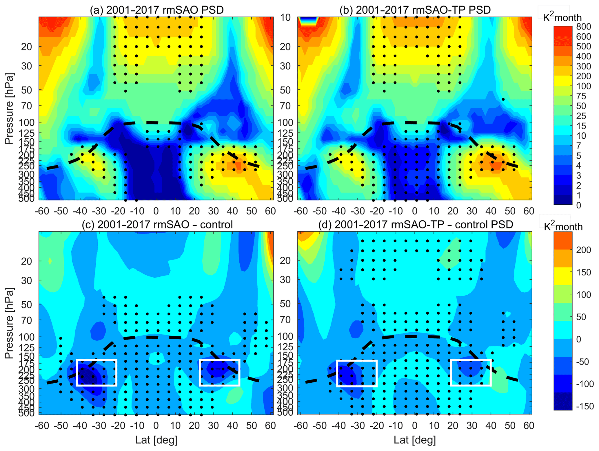
Figure 7 (a) The PSD of SAO analyzed for the period 2001–2017 based on model simulation with removed SST-SAO (rmSAO). (b) Same as (a), but for the simulation with removed SST-SAO in the Tropics (rmSAO-TP). The dots mark the significant area at 95 % level. (c) The difference of SAO PSD between the rmSAO and the control simulations (rmSAO – Control) for the period 2001–2017. (d) Same as (c), but for the difference between the rmSAO-TP and the control simulations (rmSAO-TP – Control). The black dots mark areas with significant differences of the two time series at 95 % level based on t-test. The dashed black lines mark the tropopause height calculated with GNSS RO data.

Although the UTLS-SAO is still significant in the rmSAO and rmSAO-TP simulations, the magnitudes of the UTLS-SAO in the two sensitive simulations are significantly reduced (Figs. 7c–d). Compared with control simulation, the magnitude of rmSAO simulation is reduced by 31 % for NHM and 55 % for SHM (rectangular box in Fig. 7c). The averaged magnitude reduction of rmSAO-TP simulation is 14 % in NHM and 41 % in SHM (rectangular box in Fig. 7d). Such a reduction of SAO PSD caused by removing SST-SAO is larger in the SHM and NHM than in the Tropics. This clearly shows that the SST-SAO modifies the strength of the SAO in the UTLS.

This result can also be confirmed by the averaged seasonal cycle of the extracted UTLS-SAO signal as shown in Fig. 8a. To compare the amplitude of SAO signals in model simulations, we extracted SAO signals (5–7 months) using the 1-D wavelet Morlet transform (Lilly and Olhede, 2009, 2012). As shown in Fig. 8a, the averaged amplitude of the rmSAO simulation (blue lines) is smaller than the control simulation (red lines) (11 %), and the amplitude of the rmSAO-TP simulation (dash black lines) is slightly weaker than the control simulation (1 %). This demonstrates that the SST-SAO in extratropical regions for the UTLS-SAO in NHM is more important. Reduction of the SAO amplitude related to removing SST-SAO is more evident in the SHM (Fig. 8b) compared to that in NHM. Compared with the control simulation, the averaged amplitude of the rmSAO and rmSAO-TP simulation is reduced by 33 % and 29 %, respectively. This might be related to the relatively large area of ocean in the SH compared to the NH. Anyway, a connection has been established between the surface and the UTLS SAO, and it is obvious that the SST-SAO significantly influences the UTLS-SAO.

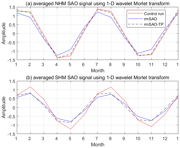
Figure 8 The average extracted SAO signals (5–7 months) based on 1-D wavelet Morlet transform for the Northern Hemisphere mid-latitudes (NHM) (a) and for the Southern Hemisphere mid-latitudes (SHM) (b). The red, blue and dashed black lines are results of the control, rmSAO and rmSAO-TP runs, respectively.

To further find out through what processes of the SSTs modifies the UTLS-SAO, the thermal budget analysis is applied to the three model simulations. Figure 9 shows a comparison of the thermal budget in the UTLS between the two sensitivity simulations and the control simulation. In the NH, the total heating rates are significantly reduced from May to July, which is mainly caused by the weaker dynamical and moist heating in the two sensitivity simulations. From August to September, the reduction of moist heating is also evident but is offset by less radiative cooling. In October, the negative values of the total heating rates are also reduced in the sensitivity simulations of rmSAO due to the reduced radiative cooling. During boreal winter, the impact of removing SST-SAO is not significant.

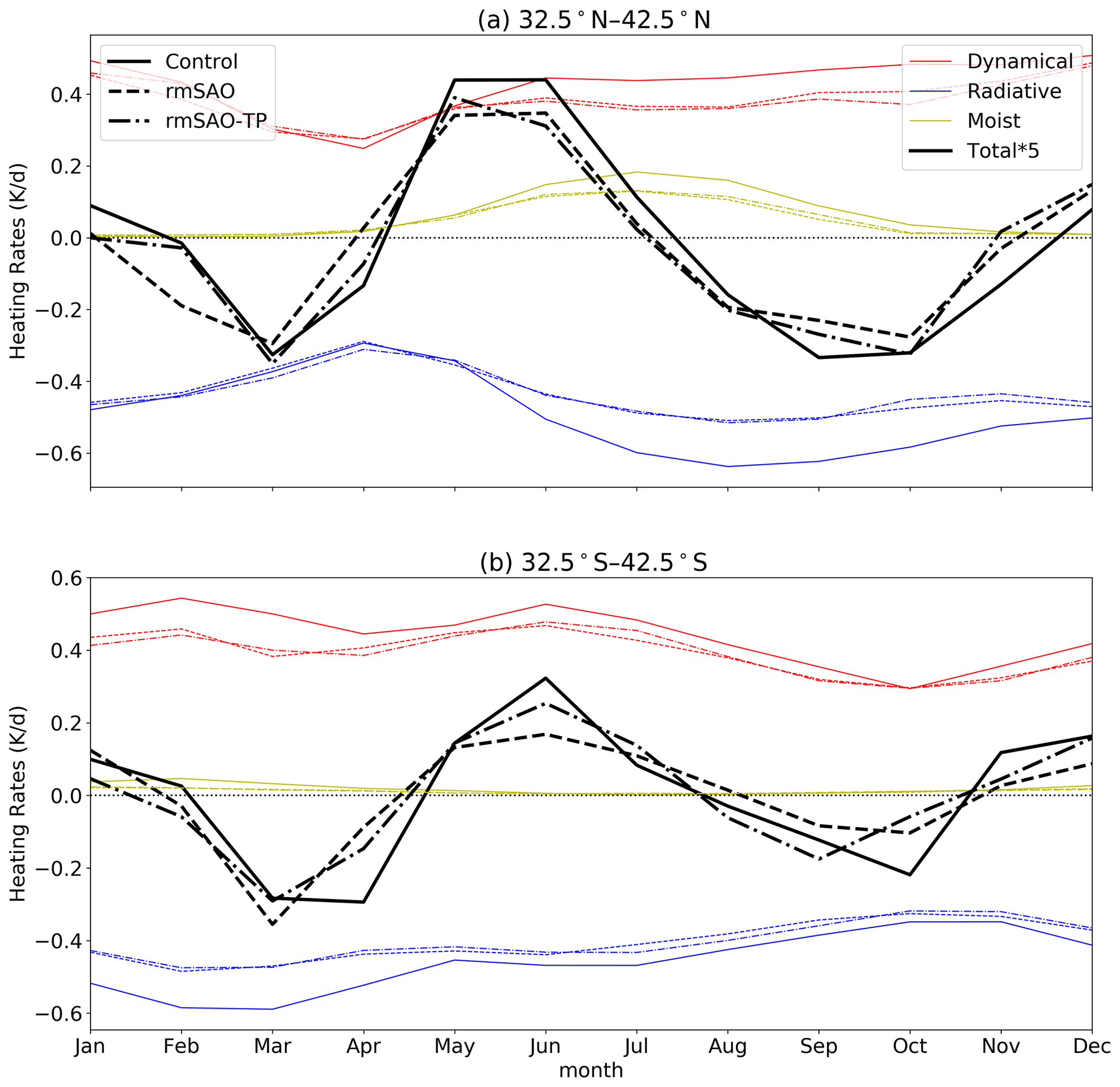
Figure 9 Annual cycle of the heating rates at 200 hPa averaged around the Northern Hemisphere mid-latitudes 32.5–42.5^∘ N (a) and the Southern Hemisphere mid-latitudes 32.5–42.5^∘ S (b). The red, blue and yellow lines indicate the heating rates related to dynamics, radiation and condensation processes, respectively. The total heating rates, which are the sum of the dynamical, radiative and moist heating rates, are illustrated by black lines. The solid, dashed and dotted-dashed lines indicate data from the control, rmSAO and rmSAO-TP simulations, respectively.

In the SH, the total heating rates are reduced overall and especially significantly reduced in austral summer (November–December). This is related to the weaker dynamical and moist heating, although it is partly offset by less radiative cooling. In austral winter, the changes in total heating rate are not significant either. The negative values of the total heating rate are also reduced in the sensitivity simulations due to the reduced radiative cooling in April, but not in March. In summary, the UTLS-SAO is modified by the SST-SAO mainly through its modification to the summer time moist heating, dynamical heating and autumn radiative cooling.

4 Conclusions

Variability of zonal mean temperatures over 500–10 hPa is analyzed based on high-quality GNSS temperature measurements and reanalysis data (MERRA2 and ERA5) covering 2001–2017. All data sets show a good agreement and ERA5 has the best agreement with GNSS RO data. The model simulations have also good agreement with other data sets except in the tropical region. Our results confirm the tropical and subtropical SAO of temperature in the upper troposphere as reported by previous studies (Loon and Jenne, 1969). In addition, we also find a significant SAO of temperature in the lower stratosphere (just above the tropopause and from 70 to 30 hPa) in the mid-latitudes of both hemispheres. From the PSD of the SAO of temperature, the SAO signal is most pronounced from the subtropics to mid-latitudes (22.5–42.5^∘) in the UTLS region (250–175 hPa). The SAO of temperature with maxima in February and July/August in the NH/SH mid-latitudes in the UTLS is observed. Furthermore, the SAO signals are likely related to both moist and dynamical processes.

The explanation of the SAO of temperature in the UTLS is given by a thermal budget analysis. In the NH, the first temperature peak in February is mainly related to the dynamical heating while the second peak in July is caused by a combination of moist and dynamical processes. The temperature peaks follow the transitions of total heating rates by definition, and the moist processes delay the transition of total heating rate from positive to negative in July. In the SH, both the dynamical and moist processes contribute to the temperature peak in austral summer, while the temperature maximum in winter (August) is mainly related to dynamical heating. The further energy budget analysis indicates that the vertical transportation of water vapor and subsequent condensation in the upper troposphere is much stronger and leads to a stronger peak of temperature in the summer season in the NHM. Through the thermal budget analysis, we also find that the UTLS-SAO in the SH can be well represented by the WACCM6 model. A significant part in the SH represented by MERRA2 model cannot be explained by ANA, dynamical and moist processes, which indicates that the budget for the SH is not as reliable as for the NH.

Based on a series of model simulations, we analyze the relationship between UTLS-SAO and the SST-SAO. The results indicate that the amplitude of the UTLS-SAO can be significantly reduced while the SST-SAO is removed in the Tropics, and will be further reduced if the SST-SAO is removed globally. The UTLS-SAO of temperature is therefore partly modified by the SSTs, which is stronger in the SHM than in the NHM. A comparison of the thermal budget between the sensitivity simulations and the control simulation further indicates that the SST-SAO mainly modifies the UTLS-SAO through its modification to the summer time moist heating, dynamical heating and autumn radiative cooling.

The annual and semi-annual variations are the most pronounced short-term climate signals. In the past decades, numerous studies have been carried out to investigate various aspects of the semi-annual cycle in the surface and stratosphere. Few attempts have been made to analyze the SAO in the UTLS especially in the mid-latitudes. The major effort of this study not only explores the structure of the SAO in the mid-latitudinal UTLS and its relationship with thermodynamic balance but also provides the relevance between the SAO in the UTLS and SSTs by climate model simulations. However, a full mechanistic understanding of the SAO drivers in the UTLS, the predictability of the SAO in the UTLS as well as its potential impacts on surface weather and climate awaits further studies.