Radar observations of winds, waves and tides in the mesosphere and lower thermosphere over South Georgia island (54° S, 36° W) and comparison with WACCM simulations

The mesosphere and lower thermosphere (MLT) is a dynamic layer of the earth's atmosphere. This region marks the interface at which neutral atmosphere dynamics begin to influence the upper atmosphere and ionosphere. However, our understanding of this region and our ability to accurately simulate it in global circulation models (GCMs) is limited by a lack of observations, especially in remote locations. To this end, a meteor radar was deployed from 2016 to 2020 on the remote mountainous island of South Georgia (54^∘ S, 36^∘ W) in the Southern Ocean. In this study we use these new measurements to characterise the fundamental dynamics of the MLT above South Georgia including large-scale winds, solar tides, planetary waves (PWs), and mesoscale gravity waves (GWs). We first present an improved method for time–height localisation of radar wind measurements and characterise the large-scale MLT winds. We then determine the amplitudes and phases of the diurnal (24 h), semidiurnal (12 h), terdiurnal (8 h), and quardiurnal (6 h) solar tides at this latitude. We find very large amplitudes up to 30 m s⁻¹ for the quasi 2 d PW in summer and, combining our measurements with the meteor SAAMER radar in Argentina, show that the dominant modes of the quasi 5, 10, and 16 d PWs are westward 1 and 2. We investigate and compare wind variance due to both large-scale “resolved” GWs and small-scale “sub-volume” GWs in the MLT and characterise their seasonal cycles. Last, we use our radar observations and satellite temperature observations from the Microwave Limb Sounder to test a climatological simulation of the Whole Atmosphere Community Climate Model (WACCM). We find that WACCM exhibits a summertime mesopause near 80 km altitude that is around 10 K warmer and 10 km lower in altitude than observed. Above 95 km altitude, summertime meridional winds in WACCM reverse to poleward, but this not observed in radar observations in this altitude range. More significantly, we find that wintertime zonal winds between 85 to 105 km altitude are eastward up to 40 m s⁻¹ in radar observations, but in WACCM they are westward up to 20 m s⁻¹. We propose that this large discrepancy may be linked to the impacts of secondary GWs (2GWs) on the residual circulation, which are not included in most global models, including WACCM. These radar measurements can therefore provide vital constraints that can guide the development of GCMs as they extend upwards into this important region of the atmosphere.

1 Introduction

The mesosphere and lower thermosphere (MLT) is an atmospheric region that marks the transition between the neutral dynamics of the middle atmosphere and ionised processes in the thermosphere and ionosphere above (Smith et al., 2011, 2017; Jackson et al., 2019; Sassi et al., 2019). The unique features of this region set the MLT apart from other atmospheric layers (Smith, 2012), including the coldest naturally occurring temperatures at the summertime polar mesopause, enormous local dynamical variability due to atmospheric tides and planetary waves (PWs), and a residual circulation that is to first order driven by small-scale atmospheric gravity waves (GWs).

The dynamics and circulation in the MLT are important for global transport of important trace chemical species (Smith et al., 2011; Kvissel et al., 2012), including transporting NO_x and meteor smoke into the winter polar stratosphere, which can affect stratospheric ozone and surface climate (Funke et al., 2017; Garcia et al., 2017), whereas the annual formation and depletion of polar mesospheric clouds (PMCs) at the summertime mesopause has an impact on sensitive chemical processes (Thurairajah et al., 2013; Siskind et al., 2018). Neutral winds in the MLT can also have first-order effects on the impacts of space weather in the ionised atmosphere above (Jackson et al., 2019; Sassi et al., 2019).

The MLT is also where the impact of solar tides on the neutral winds is greatest. Direct solar heating of the stratosphere below causes tides to propagate upwards and grow exponentially in amplitude, leading to wind reversals in the MLT that can be up to 100 m s⁻¹ over the course of one day (e.g. Jacobi et al., 1999; Mitchell et al., 2002; Murphy et al., 2006; Vincent, 2015). Planetary scale waves, which occur at periods from 2 d to more than 16 d and can reach amplitudes up to several tens of m s⁻¹ (Schoeberl and Clark, 1980; Salby, 1981a, b), also play a key role in the dynamics of the MLT by modulating GW breaking (Holton, 1984) and through non-linear interactions with solar tides (Beard et al., 1999).

One fundamental aspect of the MLT is its strong response to the forcing due to atmospheric GWs, which results in upwelling in the middle atmosphere over the summertime pole and downwelling over the winter pole (Soloman and Garcia, 1987; Vargas et al., 2015). These adiabatic cooling and heating conditions drive the thermal structure of the atmosphere away from that expected under radiative equilibrium, leading to a global-scale pole-to-pole residual circulation from the summer pole to the winter pole in the MLT (Houghton, 1978; Holton, 1983; Becker, 2012).

The sensitivity of the residual MLT circulation to GWs makes its simulation in high-top global models especially challenging (Becker, 2012; Yasui et al., 2018; Jackson et al., 2019). The majority of GWs in global models and their generation mechanisms are sub-grid scale, and the momentum deposition and subsequent driving due to these waves must be parameterised (Alexander et al., 2010). In nearly all current GW parameterisations, however, the magnitude and direction of GW momentum that reaches the MLT is almost entirely dependent on the selected GW launch spectrum near the surface, the vertical columnar propagation of GW momentum, and filtering by the background winds below. Circulations in the MLT can therefore be highly sensitive to the tuning of these GW parameterisations in ways in which the lower atmosphere is not. Further, concepts such as oblique GW propagation (e.g. Hasha et al., 2008; Song and Chun, 2008; Choi et al., 2009; Kalisch et al., 2014), the in situ generation of GWs in the middle atmosphere from jets and fronts (Fairlie et al., 1990; Sato and Yoshiki, 2008, e.g.), and secondary GWs (Vadas et al., 2018; Vadas and Becker, 2018; Kogure et al., 2020) can change the magnitude and direction of GW momentum reaching the MLT, but these are not currently included in standard operational parameterisation schemes in most global models.

Developments of advanced models employing realistic parameterisations of subgrid-scale GW influences and high time cadence observations of neutral winds, waves, and tides in the MLT are required to make progress in this regard. Satellite observations can provide a global picture, but they lack the sampling cadence to accurately constrain short timescale variability of GW processes. Meteor wind radars (MWRs), however, offer one of the best methods for measuring the neutral winds in the MLT. By measuring the radial Doppler shift of reflected radio pulses from ionised meteor trails near 90 km altitude, MWRs can derive continuous measurements of the neutral winds in the MLT at one location (Hocking et al., 2001).

To this end, a meteor radar was installed on the remote island of South Georgia (54^∘ S, 36^∘ W) in the Southern Ocean. The radar made near-continuous measurements of neutral winds in the MLT from February 2016 to November 2020. South Georgia is located near to the global GW “hot spot” of activity in the stratosphere of the southern Andes and Antarctic Peninsula (Hindley et al., 2015; Hoffmann et al., 2013; Hindley et al., 2020), and is also an intense source of wintertime GW activity itself (Hoffmann et al., 2014; Hindley et al., 2021). Further, recent modelling and observations have indicated significant generation and propagation of 2GWs in the mesosphere and thermosphere in the region (Vadas and Becker, 2019; Heale et al., 2020; Kogure et al., 2020; Lund et al., 2020; Fritts et al., 2021; Heale et al., 2022).

The goal of this study is to use these measurements to characterise the fundamental dynamics of the MLT at this remote location. In Sect. 2 we describe the radar, satellite, and modelling data sets used in this study, and in Sect. 3 we describe a new method for the localisation of derived radar winds. There then follow five results sections: in Sect. 4 we show mean winds and temperatures over the island; in Sect. 5 we characterise the solar tides; in Sect. 6 we investigate PWs; and in Sect. 7 we investigate GW activity. Last, in Sect. 8 we compare observed winds and temperatures in the MLT to climatological dynamics from the Whole Atmosphere Community Climate Model (WACCM). Our results are discussed in Sect. 9 and we summarise the study and draw our conclusions in Sect. 10.

2 Data

2.1 The South Georgia meteor radar

A SKiYMET VHF meteor radar was installed at King Edward Point (KEP) on the island of South Georgia (54^∘ S, 36^∘ W) in the Southern Ocean in January 2016. The radar was deployed in an “all sky” configuration and consists of a single solid-state transmitter operating at 35.24 MHz with a pulse repetition frequency (PRF) of 625 Hz and 7-bit Barker code, and a five-element receiver array. Peak power is around 7.5 kW. Receiver interferometry was used for simultaneous measurement of range, zenith angle, and azimuth of ionised meteor trials and enables the height and location of these trails to be determined. The Doppler shift of the returning radio pulses can be used to infer a radial “drift velocity” for each detected trail, which can be interpreted as a radial wind vector measurement at the given height, location, and time. For a full description of the SKiYMET meteor radar system, see Hocking et al. (2001).

Figure 1 Distributions of meteor echoes detected over King Edward Point (KEP) on South Georgia. Panel (a) shows the horizontal distribution of meteor echoes on 21 June 2018, where echoes are coloured according to their time of detection (see e for colour scale), whereas (b), (c), (d) and (e) show histograms of the average height, zenith angle, horizontal (ground) range, and local time of all detected meteor echoes respectively per day for all operational days. Panel (f) shows the number of meteor echoes detected per day for each day of operation during 2016 to 2020.

An overview of the meteor trail detections by the KEP radar is provided in Fig. 1. The radial component of meteor trail drift velocities are measured between altitudes of around 70 to 110 km (Fig. 1b), centred near 90 km. The peak height of the meteor distribution is related to neutral density and can vary seasonally by a few kilometres.

Meteors are detected at angles up to ∼ 80^∘ from the zenith (Fig. 1c); however, in this study we only select meteors between zenith angles of 15 and 65^∘ (dashed lines in Fig. 1c). This is to avoid potential errors in the projection of horizontal wind from meteor echoes near the zenith, and errors in the measured height of meteor echoes at large zenith angles.

Meteors are detected in all horizontal directions, as illustrated in Fig. 1a. Receivers are blanked during each transmitter pulse to avoid saturation of the receivers, resulting in a small band of arrival times during which reflected pulses are not detected. This results in the horizontal ring between 200 and 250 km from the radar, where no drift velocity measurements can be made. Despite the island's highest mountains lying to the west and south, there is also an obstruction of detections at large zenith angles to the north east due to the proximity of the relatively small Mount Duce.

The number of unambiguous meteor detections per day is shown in Fig. 1f. The radar began collecting data on 3 February 2016, typically detecting between around 2000 and 5000 meteor echoes per day. This increased to around 4000 to 8000 meteors per day from 2017 onwards. There are some time periods during 2016, 2017, and 2019 when the radar had to be taken offline due to power limitations at the KEP base, which is supplied by a hydroelectric plant on the island; however, the use of the hydroelectric energy prevented any unwanted interference from power generators on the base. The radar was uninstalled on 25 November 2020 and is expected to be redeployed at Halley research station in Antarctica.

In this study we also use measurements from the Southern Argentina Agile Meteor Radar (SAAMER) system deployed at Rio Grande (54^∘ S, 68^∘ W) in Tierra del Fuego, Argentina, as described by Fritts et al. (2010a, b). The SAAMER radar is located around 2000 km to the west of South Georgia at the same latitude, which provides an opportunity for an investigation into eastward and westward propagating planetary wave modes in Sect. 6. Throughout the study, identical data-processing steps to derive winds are applied to the meteor detections from the SAAMER and KEP radars for consistency. Derived winds from the KEP radar have also contributed to the studies by Liu et al. (2021) and Stober et al. (2021a).

2.2 Microwave Limb Sounder

Here we use version 5 of the level 2 temperature retrieval from the Microwave Limb Sounder (MLS) (MLS, Waters et al., 2006), which flies aboard NASA's Aura satellite. Aura was launched in 2004 and is part of the “A-train” constellation, following a sun-synchronous polar orbit and crossing the Equator at 01:30 and 13:30 local time each day (Schoeberl et al., 2006). MLS measures vertical profiles of microwave emissions of the atmospheric limb in five spectral bands over the altitude range of approximately 261 to 0.001 hPa (around 10 to 100 km). Temperature and pressure are retrieved from the 118- and 239 GHz bands with an estimated temperature precision in the middle atmosphere better than 3–4 K and an accuracy of between 2 and 3 K (Livesey et al., 2015; Schwartz et al., 2008). The vertical resolution of MLS varies from around 3.6–5 km between 10 and 25 km altitude to ∼ 10 km above 40 km altitude, and the along-track spacing of the vertical profiles is approximately 170 km.

2.3 WACCM

WACCM is a comprehensive global climate model that extends from near the surface to the lower thermosphere, at around 140 km altitude. Here we use an ensemble of three WACCM simulations for the period 1950–2014 that have specified sea surface temperatures based on observations. Other external input, such as anthropogenic pollutants and volcanic emissions, is also based on the observational records. The atmospheric simulations are free-running and coupled to interactive chemistry and radiation. This specific configuration is part of the Coupled Earth System Model (CESM) version 2 (Danabasoglu et al., 2020) and was completed as a contribution to the sixth round of the Coupled Model Intercomparison Project (CMIP6, Eyring et al., 2016) using the latest version (version 6) of the model (Gettelman et al., 2019). Improvements of WACCM6 over previous versions include a finer horizontal grid (0.95 × 1.25^∘), improved atmospheric chemical processes and aerosols (Tilmes et al., 2019), an expanded database of volcanic eruptions (Neely and Schmidt, 2016), additional fluxes of energetic particles due to space weather (Marsh et al., 2007; Matthes et al., 2017), and realistic magnitudes and occurrence rates of the Quasi-Biennial Oscillation (QBO) and El Niño Southern Oscillation (ENSO). For a detailed description of WACCM version 6 and its validation, we refer the reader to Gettelman et al. (2019).

3 Methods

3.1 Improved time–height localisation of radar winds using a Gaussian weighting approach

Time–height localised measurements of zonal and meridional winds u and v from meteor radar systems are usually derived by binning the measured radial velocities of individual meteors into time–height bins (e.g. Hocking et al., 2001). Then, for all meteor echoes $i=\mathrm{1},\mathrm{2},\mathrm{\dots },N$ in each bin, a least-squares fit of the function

$$\begin{array}{}\text{(1)}& \left(\begin{array}{c}{v}_{{\mathrm{h}}_{\mathrm{1}}}\\ v_{{\mathrm{h}}_{\mathrm{2}}}\\ \mathrm{⋮}\\ v_{{\mathrm{h}}_N}\end{array}\right)=\left(\begin{array}{cc}\sin {\mathit{\theta }}_{\mathrm{1}}& \cos {\mathit{\theta }}_{\mathrm{1}}\\ \sin {\mathit{\theta }}_{\mathrm{2}}& \cos {\mathit{\theta }}_{\mathrm{2}}\\ \mathrm{⋮}& \mathrm{⋮}\\ \sin {\mathit{\theta }}_N& \cos {\mathit{\theta }}_N\end{array}\right)\left(\begin{array}{c}u\\ v\end{array}\right)+\left(\begin{array}{c}{\mathit{\epsilon }}_{\mathrm{1}}\\ {\mathit{\epsilon }}_{\mathrm{2}}\\ \mathrm{⋮}\\ {\mathit{\epsilon }}_N\end{array}\right)\end{array}$$

is performed to recover estimates of u and v, where $v_{\mathrm{h}}=v_{\mathrm{r}}/\sin \mathit{\varphi }$ is the horizontal projection of the measured radial velocity v_r of the meteor trail, ϕ is the angle from the zenith, θ is azimuth (defined clockwise from north), and ε is an error term for each meteor measurement. These time–height bins can be typically around 1–2 h in time and ∼ 3 km in height (Hocking and Thayaparan, 1997; Mitchell et al., 2002; Mitchell and Beldon, 2009). A threshold value of at least 20 meteor echoes in a bin can be applied to ensure a reliable fit (Mitchell and Beldon, 2009). Note that because meteors from all azimuths are used in this fit, and the cosine function is unique over one period, the slightly uneven distribution of meteors with azimuth in Fig. 1a does not significantly affect the results of our wind fitting method.

This method is simple and effective, but it has several important limitations, namely (1) meteors near the boundaries of the time–height bin count 100 % to the centre of the bin, but not to neighbouring bins; (2) the fit is not constrained by the fits of neighbouring bins, that is, we would not expect a wildly different value for u and v from one hour to the next to be physical, yet this is permitted by the method; and (3) in bins with low meteor counts the cutoff threshold is applied and the fit is not performed, even if the fit could be constrained by using neighbouring bins.

Here we describe a new approach to mitigate these problems. Instead of defining a time–height bin centred at time t₀ and height z₀, we define a two-dimensional Gaussian weighting function centred at (t₀,z₀). This Gaussian function has standard deviations σ_t=0.85 h and σ_z=1.275 km, which correspond to full-width-at-half-maximum (FWHM) values of 2 h and 3 km in time and height respectively. The central location of the function (t₀,z₀) is then moved through time and height in steps of 1 h and 1 km. For a given height and time at each of these steps, each meteor echo i has a weighting w_i, which is the product of its weightings in time $w_{t_i}$ and height $w_{z_i}$, given by

$$\begin{array}{}\text{(2)}& \begin{array}{rl}{w}_i& =w_{t_i}{w}_{z_i}\\ & =\exp \left({\displaystyle \frac{-(t_i-t_{\mathrm{0}}{)}^{\mathrm{2}}}{\mathrm{2}{\mathit{\sigma }}_t^{\mathrm{2}}}}\right)\exp \left({\displaystyle \frac{-(z_i-z_{\mathrm{0}}{)}^{\mathrm{2}}}{\mathrm{2}{\mathit{\sigma }}_z^{\mathrm{2}}}}\right)\end{array}.\end{array}$$

These weightings are then used to perform a weighted least-squares fit of the function in Eq. (1). The fit is performed using a weighted matrix inversion method as

$$\begin{array}{}\text{(3)}& \left(\genfrac{}{}{0ex}{}{u}{v}\right)={\left({\mathbf{X}}^{\top }({\mathbf{W}}_{\mathrm{2}}\circ \mathbf{X})\right)}^{-\mathrm{1}}{\mathbf{X}}^{\top }(\mathit{W}\circ \mathit{Y}),\end{array}$$

where X is an N×2 matrix containing the sine and cosine terms of azimuth as in Eq. (1), $\mathit{W}=\left(w_{\mathrm{1}},w_{\mathrm{2}},\mathrm{\dots }{w}_N\right)$ is an N×1 column vector containing the weightings, $\mathit{Y}=\left(v_{{\mathrm{h}}_{\mathrm{1}}},v_{{\mathrm{h}}_{\mathrm{2}}},\mathrm{\dots }{v}_{{\mathrm{h}}_N}\right)$ is an N×1 vector containing the measured horizontal velocities, and W₂ is simply an N×2 duplicate of the weighting vector W. Here, ∘ denotes elementwise multiplication (Hadamard product) between two matrices, X⁻¹ denotes the matrix inverse, and X^⊤ denotes the transpose.

Although Eq. (3) can be rearranged to be written more simply, we found that this formulation was the most efficient to solve computationally. To further improve computation speed, we only consider horizontal velocities from meteor echoes with a combined time–height weighting of w_i>0.05 (around two standard deviations) for each fit, which keeps the above matrices relatively small. This cutoff means that winds derived at least two standard deviations apart in height (± 1.7 km) or time (±2.55 h) are entirely independent.

Due to the irregular distribution of meteors in time and height, for each fit we use the same weights in the vector W to compute a weighted mean of the altitude and time to which the derived winds correspond. This is usually offset from the centres of the tim–height Gaussians because of irregular distributions of meteors, especially with height. This means that our derived horizontal winds vary smoothly and accurately with the true distribution of meteor detections in height and time, which is not necessarily the case with the traditional time–height bin approach where fixed bin centres are used, as in, for example, Mitchell et al. (2002).

3.2 Comparison with a traditional height gates approach

The new Gaussian weighting method is compared with a traditional time–height bin method in Fig. 2. Derived zonal (top) and meridional (bottom) winds from radar measurements at KEP during the period 3 to 8 May 2017 are shown for a time–height bin method (left) and the new Gaussian weighted method described above (right).

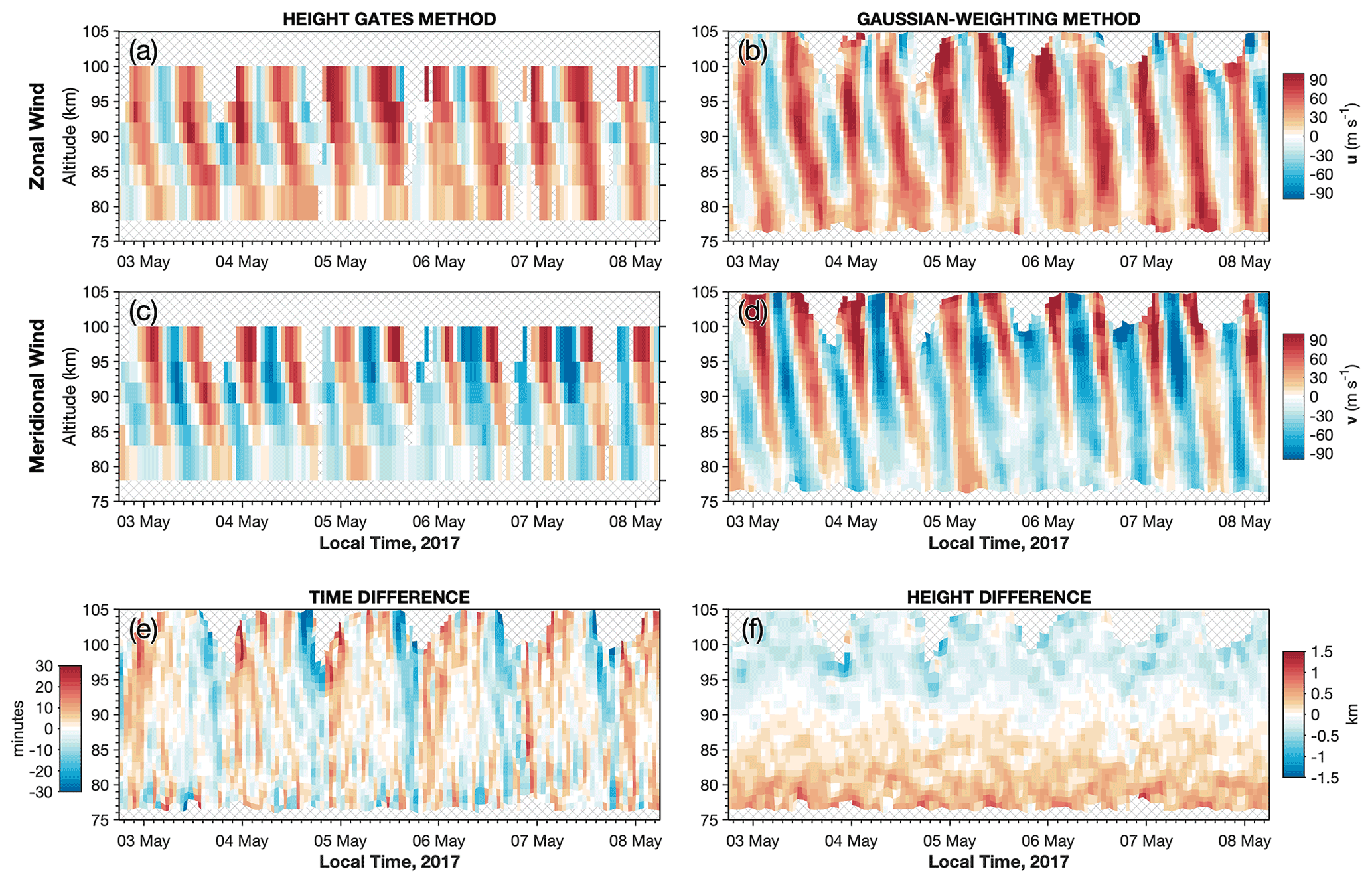
Figure 2 Derived zonal and meridional winds from the South Georgia meteor radar during May 2017 using (a, c) a traditional time–height binning approach and (b, d) the new Gaussian time–height weighting approach described here. Hatched areas show regions with too few meteors to reliably derive winds. Lower panels (e) and (f) show differences between the Gaussian-weighted mean time and height of each derived wind measurement using the new method and the time and height at the centre of the weighting function (as would be used in a traditional binning method).

The height bins chosen follow those used by Mitchell et al. (2002) and are at altitudes of 78–83, 83–86, 86–89, 89–92, 92–95, and 95–100 km. They are 2 h wide in time and are stepped along in 1 h steps. A threshold of at least 20 meteors for the fit is applied in both methods, and the hatched regions indicate where this condition is not met.

Periodic oscillations near 12 h in the zonal and meridional winds are found in Fig. 2 in both methods. This is the semidiurnal solar tide, which is dominant at this latitude and season.

Several advantages to the new Gaussian weighting method are found. First, the full altitude range of the available measurements is revealed and reliable winds are automatically found at higher and lower altitudes during the morning (local time) when meteor counts are high. On some occasions, we found that winds can be derived up to 110 km altitude (not shown) with a realistic tidal phase progression with height, suggesting that altitude independence can be maintained with this method despite low meteor counts.

Second, winds are successfully derived by the Gaussian weighting method for time periods where too few meteors were detected to ensure a reliable fit using the traditional method, such as during the afternoon of 6 May 2017. This is because additional meteor echoes, which would have been in adjacent bins in the traditional method, are available to constrain the fit in Eq. (3). These missing periods cannot be filled in simply by the interpolation of the surrounding wind measurements. This also has the advantage of reducing spurious wind fits during periods of low meteor counts, because the inclusion of neighbouring meteor measurements helps to prevent unphysically large changes in wind between two adjacent time steps or height levels.

We note that the wind measurements in the Gaussian weighting method appear to warp away from a regular time–height grid at upper and lower altitudes. This is due to the derived winds being correctly allocated to the weighted mean time and height of the available meteors, which is not considered in the traditional method.

This effect is quantified in panels (e) and (f) of Fig. 2, which show differences between the time and altitude at the centre of the Gaussian function (as in a binning approach) and the average Gaussian-weighted time and altitude of the meteors used for the wind derivation. We can see that, due to the irregular distribution of meteor echoes with time and height, if the times and heights of derived values are simply assigned to the centre of a “bin” this can result in up to around 20 min or 1 km from the correctly weighted time–height average of the meteor echo locations. Accounting for this time offset is less important for the mean winds, but it can be important for accurately fitting the phases of the solar tides, especially higher order tidal modes.

This new approach can help to extend reliable wind measurements to the full vertical extent of meteor echo detections, allow for derived winds on shorter time scales, more accurately derive the time and height of derived quantities, and is applicable to any meteor wind radar system.

4 Large-scale winds and temperatures in the MLT over South Georgia

The general dynamics of the large-scale zonal and meridional winds over South Georgia are characterised in the power spectra in Fig. 3, which shows a normalised Lomb–Scargle periodogram of hourly winds at 90 km altitude for the period February 2016 to November 2020 inclusive. The large semidiurnal solar tide S₂ dominates, with the diurnal (S₁) and terdiurnal (S₃) tides showing roughly equal amplitudes at this latitude. At periods longer than 1 d, peaks near 2, 5, 10, and 16 d are found, which correspond to known planetary wave periods, although other periodicities are also present (e.g. quasi-6 d). At periods shorter than the inertial period (f∼14.8 h at this latitude) but excluding tidal periods, the spectra are dominated by gravity waves and follow a $-\mathrm{5}/\mathrm{3}$ gradient (solid red line) as expected from theory (e.g. Smith et al., 1987). A significant peak is also found near 12.4 h, which likely corresponds to the semidiurnal lunar tide M₂, suggesting that this radar dataset at South Georgia could be useful for investigating lunar tides, although the diurnal lunar tide M₁ appears to be very weak at this latitude.

Figure 3 Normalised power spectra of the hourly zonal (a) and meridional (b) winds at 90 km altitude measured by the South Georgia meteor radar for the period 2016 to 2020. Annotations show peaks corresponding to solar tides S_1–4, lunar tides M_1–2 and planetary waves, where shaded grey regions for the latter show an approximate range of periods. The dashed horizontal line shows the 90 % confidence level, f denotes the inertial period (∼ 14.8 h) at 54^∘ S, and the black line illustrates an idealised $-\mathrm{5}/\mathrm{3}$ power law for gravity waves.

It should be noted in Fig. 3 that the standard 90 % significance level shown inherently assumes a flat frequency spectrum, which is not the case for most atmospheric spectra. Consideration therefore should also be given to the relative size of peaks compared with their neighbouring frequencies, such as for the quardiurnal (S₄) solar tide, but this is challenging to quantify.

Further, there is an apparent change in the slope of the GW part of the spectrum at periods less than around 4 h, which is due to our sensitivity limits. Although we sample the winds hourly (which implies a 2 h Nyquist resolution limit), the fact that we apply a sliding Gaussian window with a FWHM equal to 2 h as described in Sect. 3.1 above means that we are not sensitive to oscillations with periods less than around 2–4 h, meaning that this part of the spectrum in Fig. 3 is likely to be indistinguishable from retrieval noise and measurement error.

To explore the dynamics of the MLT on monthly timescales, Fig. 4 shows derived monthly zonal (top) and meridional (bottom) winds against altitude for 2016 to 2020. These winds are derived as monthly composite days where, for each month, all meteor measurements in that month are assumed to occur on the same day. Hourly winds are fitted via the method in Sect. 3.1 and the average wind for each monthly composite day is found. The rightmost panels in Fig. 4 show a composite year using the same 30 d sliding window, except that all measurements are assumed to occur in the same year.

Figure 4 Monthly mean zonal and meridional winds (a–d) in the MLT from radar measurements over South Georgia during 2016 to 2020. Panels (e) and (f) show monthly mean temperatures from MLS satellite measurements. Rightmost panels show winds and temperatures derived from an average (composite) year using all meteor detections and all temperature measurements during 2016 to 2020.

The zonal winds in Fig. 4a, b indicate a clear annual cycle, with eastward winds in austral winter and a strong wind shear that descends in altitude during summer. The onset and descent of this summertime wind shear follows a characteristic “triangular” pattern when plotted on time–height axes, with a rapid (∼ 1 month) onset during spring followed by a gradual descent in altitude throughout summer into autumn over approximately 5 to 6 months. This is consistent with other meteor radar wind observations at high midlatitudes in both hemispheres (e.g. Fritts et al., 2010b; Sandford et al., 2010; Stober et al., 2021c). The vertical gradient of the zonal wind in summer is particularly strong, from around −20 m s⁻¹ (westward) to up to +40 m s⁻¹ (eastward) over only 10 to 15 km altitude.

In the monthly mean winds shown here, there does not appear to be a significant change in the observed zonal winds over South Georgia during the southern sudden stratospheric warming (SSW, e.g. Rao et al., 2020) in September 2019. This is likely because, as shown recently by Liu et al. (2021), wind responses occurred on timescales of up to around 10 d, which are shorter than those shown in the results here.

Meridional winds in Fig. 4c, d are northward and up to 20 m s⁻¹ during summer, and southward wind during winter. This flow is part of a summer-to-winter pole circulation in the MLT that is sometimes referred to as the mesospheric branch of the Brewer–Dobson circulation (BDC) as described by Murgatroyd and Singleton (1961), although the BDC is most significant in the tropical troposphere and lower stratosphere. The summertime northward flow maximises near 80 km altitude, whereas the wintertime southward flow is weaker but persists for approximately 1 to 2 months longer than the summertime conditions. Interestingly, during 2016, 2017, and 2020 there is a brief reversal of the southward flow to northward during winter. This also occurs at altitudes above 90 km and 95 km during 2018 and 2019 respectively. This weak wintertime reversal was also found in radar observations at high latitudes in both hemispheres by Sandford et al. (2010), which could suggest a weak semiannual modulation of the summer-to-winter pole flow in the MLT. This modulation could be connected to the mesospheric component of the tropical semiannual oscillation (SAO, e.g. Smith et al., 2017; Ern et al., 2021). The weak meridional wind reversal seen here during winter coincides with the eastward phase of the tropical SAO in the mesosphere, which is known to be out of phase with the stronger stratospheric component of the SAO. Another explanation for this could be shifts in the amplitude and/or phase of quasi-stationary planetary waves in the winter stratosphere and lower mesosphere, which could play a major role in modulating the flow observed at a single location.

Observed winds during the winter of 2016 show differences from the other years in this 5-year period. The zonal winds are more than 10 m s⁻¹ weaker on average below 90 km altitude during July–August, and more than 20 m s⁻¹ weaker than the following year during June–July above 90 km altitude. Meridional winds during 2016 also show the largest wintertime reversal from southward to northward and back to southward again during June to October. Although meteor counts were lower than those for other years (Fig. 1f), the sliding 30 d composite window still provides at least ∼ 30 000 measurements from which to fit winds in a given composite day; thus, our results are unlikely to be affected by this.

The reason for the unusual winds observed during 2016 is not immediately clear. It is known that the El Niño Southern Oscillation (ENSO) and Quasi-Biennial Oscillation (QBO) can have a significant effect on MLT dynamics (e.g. de Wit et al., 2016; Laskar et al., 2016; Sun et al., 2018). In 2016, ENSO was in an unusually strong warm phase, and there was an unprecedented disruption of the QBO (Osprey et al., 2016). As mentioned above, it is also likely that changes in quasi-stationary planetary waves in the winter hemisphere play a major role in the observed interannual variability. A study that could explore a possible link between these dynamical processes and the reduced wind speeds observed over South Georgia in 2016 could provide valuable information into coupling processes between atmospheric layers. Such a study would, however, require a longer time series of observations for sufficient statistics and a numerical modelling component for exploring a plausible mechanism, and so is outside the scope of this article.

The bottom panels of Fig. 4 show monthly mean temperatures in the MLT from MLS satellite observations, averaged over a horizontal region within a 400 km radius of the island for each height level, which is close to the size of the horizontal collecting area of the meteor radar. These show the annual cycle of temperatures in the MLT, including the cold summertime mesospause where temperatures fall below 160 K between 95 and 100 km altitude around the summer solstice, despite the polar mesosphere being subject to constant sunlight. This temperature structure is different from that expected under radiative equilibrium (Geller, 1983), and is instead driven away from this state by the effects of atmospheric waves (e.g. Smith, 2012; Becker, 2012). The wintertime mesopause is warmer and occurs above 105 km altitude each year.

5 Solar Tides

The diurnal variability of the MLT region is dominated by solar tides, which have periods that are integer fractions of 1 d. Tides measured in the MLT have typically propagated upwards from the stratosphere and troposphere below, where the atmospheric response to solar heating is largest, rather than being directly excited in the MLT (Smith, 2003, 2012). As shown recently by Dempsey et al. (2021), tidal amplitudes and variability at high latitudes are not always well simulated in numerical models; thus, characterising the tidal magnitudes and seasonal variability here can have value.

To characterise the solar tides, we use a sliding composite day method (sometimes referred to as a superposed epoch analysis), which is a common approach to meteor radar measurements (Davis et al., 2013). Here, meteors that are detected within a specified range of days before and after a specific day are assumed to have been measured on that same day. The Gaussian-weighted wind-fitting method outlined in Sect. 3.1 is then followed to create a composite day of hourly zonal and meridional winds at each height level for all measurements in this time window.

We then fit sinusoids of 24, 12, 8, and 6 h to these hourly winds simultaneously. This is done by assuming that the daily hourly winds for each height consist of a sum of four sinusoidal waves at tidal periods n = 24, 12, 8, 6 h described by constants A_n and B_n oscillating around a mean background wind C. For the hourly zonal wind u(t) at one height, this can be written as

$$\begin{array}{}\text{(4)}& u\left(t\right)=\left(\begin{array}{ccc}\mathcal{A}& \mathcal{B}& C\end{array}\right)\left(\begin{array}{c}\cos (\mathrm{2}\mathit{\pi }t/\mathit{\tau })\\ \sin (\mathrm{2}\mathit{\pi }t/\mathit{\tau })\\ \mathrm{1}\end{array}\right),\end{array}$$

where t contains the weighted average times of the hourly wind measurements in hours, $\mathcal{A}=\left(A_{\mathrm{24}},A_{\mathrm{12}},A_{\mathrm{8}},A_{\mathrm{6}}\right)$ and $\mathcal{B}=\left(B_{\mathrm{24}},B_{\mathrm{12}},B_{\mathrm{8}},B_{\mathrm{6}}\right)$ are row vectors containing the tidal amplitude coefficients for the cosine and sine terms respectively, C is the mean, and $\mathit{\tau }=\left(\mathrm{24},\mathrm{12},\mathrm{8},\mathrm{6}\right)$ is a column vector containing tidal periods in hours. The two matrices in Eq. (4), therefore, have sizes 1×9 and 9×24 respectively. By taking the transpose of both matrices on the right-hand side, we can arrange Eq. (4) as P=Mx and solve as $x=M^{-\mathrm{1}}P$ to yield the tidal coefficients. Amplitudes and phases for each tidal period $n=\mathrm{24},\mathrm{12},\mathrm{8},\mathrm{6}$ are given by $\sqrt{A_n^{\mathrm{2}}+B_n^{\mathrm{2}}}$ and ${\tan }^{-\mathrm{1}}(A_n/B_n)$ respectively, and C is the mean background wind for the composite day. We then repeat this process to fit meridional tidal coefficients to the composite day meridional winds v(t).

Figure 5 shows the monthly amplitudes and phases of the zonal and meridional tidal components, averaged for the period 2016 to 2020. Monthly composite tidal amplitudes and phases for the full period 2016 to 2020 are also included in Figs. S1 and S2 in the Supplement.

Figure 5 Zonal and meridional wind amplitudes and phases of the diurnal (24 h), semidiurnal (12 h), terdiurnal (8 h), and quardiurnal (6 h) solar tides in the MLT over South Georgia averaged for the years 2016 to 2020. Tidal amplitudes and phases are fitted to composite daily winds derived using a sliding 30 d time window of measurements. Phases are given in hours since midnight local time. Hatched regions show where the measured tidal amplitudes are low (less than 5 m s⁻¹ for the 24, 12, and 8 h tides, and less than 2.5 m s⁻¹ for the 6 h tide) and phase measurements may less reliable.

Our results show that the semidiurnal tide is dominant at this latitude, especially during winter, with amplitudes that can reach up to 60 and 80 m s⁻¹ in the zonal and meridional directions respectively during April to May each year, broadly consistent with previous studies (e.g. Murphy et al., 2006; Conte et al., 2017). The intra-annual variability of the semidiurnal tide is broadly characterised by an “equinox high” and “solstice low”, although we find a lag of around 1.5 months in the tidal maxima after the solstice and equinox dates. We also find that the meridional component of the semidiurnal tide is consistently around 25 % to 35 % larger than the zonal component throughout the year.

The amplitudes of the diurnal and terdiurnal tides in Fig. 5a, b and i, j are weaker, reaching values up to 15 and 10 m s⁻¹ respectively. The diurnal tide maximises in summer, where the meridional component is as much as three times as large as the zonal. Largest average values for the meridional component are up to 15 m s⁻¹ above 100 km altitude during December to March, but can be as large as 25 m s⁻¹ during individual years. The altitude structure of the diurnal tide is also somewhat opposite to the semidiurnal, maximising above 100 km and below 85 km, whereas the semidiurnal tide maximises in between these altitude ranges.

The amplitude of the terdiurnal tide broadly follows the annual and semiannual cycle of the semidiurnal tide, especially in the meridional direction in Fig. 5j, with maxima of around 5 to 10 m s⁻¹ around May and September. The autumnal maximum of the terdiurnal tide is broadly consistent with averaged amplitudes from December to March from satellite measurements by Smith (2000) at latitudes near 60^∘ S. The timing of this maximum is an interesting result, because it has been suggested (Moudden and Forbes, 2013) that the observed terdiurnal tide could primarily be the result of non-linear interaction of the diurnal (D) and semidiurnal (S) tides, rather than by direct solar excitation. Moudden and Forbes (2013) used global satellite measurements from SABER to decompose the terdiurnal tide (T) into its constituent eastward (E) and westward (W) propagating modes and zonal wavenumbers (1, 2, …, N). They found that the dominant mode of the terdiurnal tide was TW3, which could be the result a non-linear interaction between DW1 and SW2.

However, as discussed in detail by Lilienthal et al. (2018), excitation mechanisms of the terdiurnal tide, in particular the role of direct solar heating versus non-linear interactions is still under debate. In the modelling studies of Lilienthal et al. (2018) and Lilienthal and Jacobi (2019), they found that the solar heating was dominant, but that non-linear interactions could become significant at midlatitudes during winter. The wintertime maximum of the terdiurnal tide in our results could therefore be consistent with the results of both Moudden and Forbes (2013) and Lilienthal and Jacobi (2019) and suggest that both factors could be important during this time.

The quardiurnal (Fig. 5) tide at this latitude is weaker in amplitude than the other dominant modes, reaching maxima of only 5 and 2.5 m s⁻¹ in the zonal and meridional directions respectively during April to May. These amplitude values and seasonality, however, are broadly consistent with measurements of the quardiurnal tide in the northern hemisphere by Smith (2004) and Pancheva et al. (2021). This is a useful result, because the quardiurnal tide can be challenging to measure due to its small amplitudes, which often fall below measurement accuracy.

The zonal and meridional tidal phases, which we define as the local time of the first positive (eastward for zonal, northward for meridional) wind maximum in hours, are shown in the two right-hand columns of Fig. 5. White hatched areas indicate regions where measured tidal amplitudes are relatively low; thus, measured phases may be less reliable. A seasonal cycle is revealed for each of the four tidal modes considered here. One interesting result is that when the amplitudes of each tide are large, the measured phases exhibit a $\frac{\mathit{\pi }}{\mathrm{2}}$ phase lag between the zonal and meridional components, where the meridional phase lags behind the zonal by a quarter cycle. This is consistent with the circular polarisation and anticlockwise rotation of the tidal wind vector (when viewed on a hodograph), which is indicative of an upwardly propagating tide in the southern hemisphere. Further, when the tidal amplitudes are relatively large, there also appears to be a negative change in tidal phase with increasing height, which is again consistent with an upwardly propagating tide. This is the case for the diurnal tide during late summer and the semidiurnal and terdiurnal tides during winter.

This implies that, when tidal amplitudes are relatively large, our phase measurements are robust and realistic. This phase consistency is especially encouraging for our measurements of the terdiurnal tide, whose small amplitude generally makes accurate measurements challenging. However, during time periods when tidal amplitudes are relatively small (hatched areas in Fig. 5), this phase consistency breaks down, indicating that our tidal phase analysis is poorly constrained during these times.

6 Planetary Waves

In this section we investigate PWs in our radar wind observations over South Georgia. PWs are global-scale propagating waves with small zonal wavenumbers and periods of order days that arise as one of several rotational Hough modes in the earth's atmosphere, where conservation of angular momentum is the restoring force that governs the oscillation (e.g. Smith, 2012). Note that we can only investigate travelling PWs using our single-site measurements here and not stationary PWs, which we are unable to separate from the large-scale flow.

To characterise the spectral properties of travelling PWs here, we use the S-transform (Stockwell et al., 1996). The S-transform is a spectral analysis technique that can provide time-frequency localisation of the complex spectrum, allowing us to probe the temporal variability of various periods present in our wind measurements. This is particularly useful for the study of PWs, whose amplitudes and periods may vary significantly over just a few cycles. The spectral coefficients of the S-transform are also directly related to wave amplitudes without the need for further scaling, which is an advantage over traditional forms of the continuous wavelet transform (CWT). The S-transform has also been used previously by Fritts et al. (2010b) to characterise PWs in meteor radar wind observations. Here we use the S-transform analysis of Hindley et al. (2019), which follows the same analytic approach as that of Stockwell et al. (1996) but includes several scaling options and significant improvements in computation speed. We select a scaling parameter of c=1 to provide a fair balance between temporal and spectral localisation (see Hindley et al., 2019) meaning that any measured PW amplitudes can be considered to be “averaged” over approximately one wave cycle.

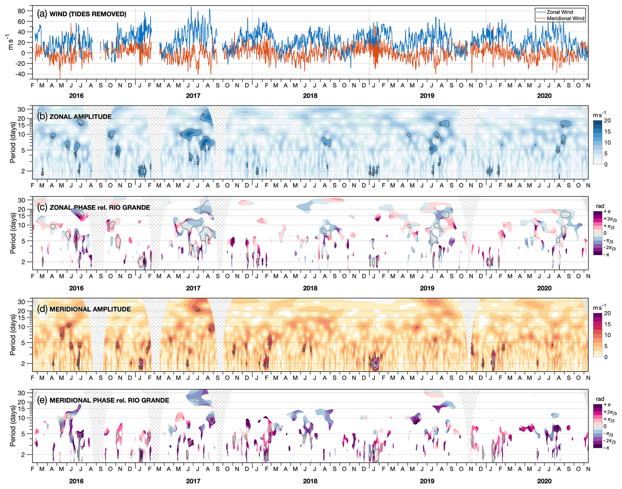
Figure 6 S-transform spectral analysis of planetary wave periods over South Georgia from meteor radar observations. Panel (a) shows 6-hourly zonal (blue) and meridional (orange) radar winds at 95 km altitude. Panels (b) and (d) show measured S-transform amplitudes of these zonal and meridional winds respectively, whereas (c) and (e) show the corresponding co-varying phase relative to 6-hourly wind measurements from the SAAMER meteor radar located 2000 km to the west. Here, a positive (negative) phase shift indicates a dominant eastward (westward) propagating PW mode. Hatched regions in (b) and (c) indicate unusable regions of spectral analyses due to missing data periods and “cone-of-influence” effects around these times.

Figure 6a shows 6-hourly zonal and meridional winds at 95 km altitude for the time period 2016 to 2020. These winds are found by subtracting a daily fit of the 24, 12, 8, and 6 h solar tides as described in Sect. 5, and then low-pass filtering the residual winds with a cutoff of 6 h. Figure 6b, d show PW amplitudes measured by our S-transform analysis for periods from 1.75 to 35 d. Hatched areas indicate missing time periods (due to the radar being offline) and unusable regions due to the “cone-of-influence” effect.

Periodic signals at known PW periods near approximately 2, 5, 10, and 16 d are observed. During December to February each year, a periodicity near 2 d is observed in both the zonal and meridional directions with amplitudes exceeding 10 m s⁻¹. This is indicative of the Q2DW, which maximises during summer at high midlatitudes (e.g. Tunbridge and Mitchell, 2009). The largest measured amplitudes of the Q2DW seen here occur during January 2019, exceeding 15 and 30 m s⁻¹ in the zonal and meridional directions respectively. We found that the phase of the large-amplitude meridional Q2DW during this time (not shown in Fig. 6) is consistently around 03:00 local time throughout January 2019. Interestingly, the phases of the meridional components of the diurnal and semidiurnal tides shown in Fig. 5 are also both around 03:00 to 06:00 local time, which could suggest a phase locking of the tides and the Q2DW, which could lead to the large amplitudes observed.

Planetary wave activity at longer periods near 5, 6, 10, 16, and 20 d is also observed in both the zonal and meridional directions in Fig. 6b, d, with amplitudes greater than 10 m s⁻¹ persisting for more than a month on occasions. These periodicities likely correspond to presence of the quasi 5 d wave (Q5DW, Day and Mitchell, 2010a), the quasi 6 d wave (Forbes and Zhang, 2017; Yamazaki et al., 2020), the quasi 10 d wave (Q10DW, Forbes and Zhang, 2015; Wang et al., 2021), and the quasi 16 d wave (Q16DW, (Day and Mitchell, 2010b). Each of these PWs typically reach a maximum at high midlatitudes during mid to late winter, which is consistent with each of the previous studies listed above. One interesting time period occurs during June to August 2017, where there is an apparent superposition of periods near 6–8, 10–11, and 20–21 d in the zonal wind measurements, each up to 15 m s⁻¹ in amplitude. It is likely that these periodicities correspond to the Q5DW, Q10DW, and Q16DW respectively, but their periods may be modulated due to non-linear interactions with each other. In the subsequent years 2019 and 2020, these PWs are measured again during June to August but with periods closer to their traditional periods near 5, 10, and 16 d, where they occur at slightly weaker amplitudes near to 10 m s⁻¹. For these periods, the measured zonal wind PW amplitudes are almost always larger than the meridional, which is in contrast to the Q2DW amplitude during summer. We should note that there also exists a quasi 4 d wave (Yamazaki et al., 2021) that grows and maximises during summer at high latitudes, and this may be apparent during June 2017 in our results.

Eastward and westward propagating modes

Planetary waves observed at a single location can consist of a superposition of eastward (E) and westward (W) propagating modes, each with a zonal wavenumber, e.g. 1, 2, 3. To investigate this we combine our results at KEP with wind measurements at the same altitude from the SAAMER meteor radar system at Rio Grande, in Tierra del Fuego (TDF), Argentina (54^∘ S, 68^∘ W) to provide information on these eastward and westward propagating modes. We apply the same S-transform analysis to mean winds from TDF, and then find the co-varying PW signals between the two sites as $C_{\mathrm{a},\mathrm{b}}=S_{\mathrm{a}}{S}_{\mathrm{b}}^{*}$, where S_a and S_a are the S-transform spectra for TDF and KEP respectively, C_a,b is the complex covariance spectrum and $S_{\mathrm{b}}^{*}$ denotes the complex conjugate. We then find the phase difference of any co-varying signals between the two sites as ${\tan }^{-\mathrm{1}}\left(\frac{\mathbb{R}\left(C_{\mathrm{a},\mathrm{b}}\right)}{\mathbb{I}\left(C_{\mathrm{a},\mathrm{b}}\right)}\right)$, where ℝ and 𝕀 denote the real and imaginary parts of C_a,b.

The results of this analysis are shown in Fig. 6c, e for the zonal and meridional direction respectively. Here, a positive (negative) phase shift indicates a dominant eastward (westward) propagating mode. The KEP and TDF radars are located approximately 2000 km apart, which is around $\mathrm{1}/\mathrm{12}$ of the circumference of the earth at this latitude (∼ 23 500 km). Therefore, measured phase differences near $\frac{\mathit{\pi }}{\mathrm{6}}$, $\frac{\mathit{\pi }}{\mathrm{3}}$, and $\frac{\mathit{\pi }}{\mathrm{2}}$ correspond to dominant zonal wavenumbers of 1, 2, and 3, and so on. Regions where the measured PW amplitude at KEP is less than 5 m s⁻¹ are coloured white, and the 10 m s⁻¹ contour lines from panels (b) and (d) are added to indicate when PW activity is significant.

We find that the PW periods near 5, 10, and 16 d that occur at large amplitudes in the zonal direction during winter in Fig. 6b consistently correspond to small negative (blue) phase shifts in Fig. 6c, which indicates a dominant westward propagating mode for these PWs. For example, during June to September 2019 the measured phase shift PWs near 5, 10, and 16 d are between $\frac{-\mathit{\pi }}{\mathrm{6}}$ and $\frac{-\mathit{\pi }}{\mathrm{3}}$, indicating dominant modes close to W1 and W2 (westward modes 1 and 2). The westward propagating Q10DW mode here is consistent with the results of Wang et al. (2021), who found evidence of a strong W1 mode of the Q10DW using meteor radar winds from Rothera and McMurdo, Antarctica during the months leading up to the 2019 southern sudden stratospheric warming (SSW Rao et al., 2020, ,). During August to September 2020 in Fig. 6c, the small negative phase shift corresponding to the Q16DW is indicative of a dominant W1 mode, as predicted by Salby (1981b).

We should note that this analysis can only determine the dominant PW mode at any given time and period, and with only two sites we cannot unambiguously determine PW modes due to possible aliasing effects. However, because our two sites are relatively close together, this means that aliasing is unlikely for PW zonal wavenumbers smaller than perhaps 4 or 5. On the other hand, because the sites are so close, the phase shift for zonal wavenumber 1 is relatively small, $\sim \frac{\mathit{\pi }}{\mathrm{6}}$, which may be susceptible to measurement error.

The measured phase shifts for the Q2DW during summer each year in Fig. 6d, e also exhibit some unexpected results. Tunbridge et al. (2011) and Pancheva et al. (2018) used MLS temperature measurements to provide a global decomposition of the Q2DW into its eastward and westward propagating modes. They found that the large summertime amplitudes at high midlatitudes primarily correspond to the westward propagating zonal wavenumbers 2 and 3 (W2 and W3) modes. During winter, both studies also showed evidence of a weaker eastward propagating zonal wavenumber 2 (E2) mode of the Q2DW, which, although maximising near the stratopause, was visible near 90 km. The MLS observations in Pancheva et al. (2018) were also supported by numerical simulations from the NOGAPS-ALPHA model, which supported the observed seasonal change in the dominant modes (Pancheva et al., 2016).

In our results, however, we do not find a consistent phase shift during summer for the Q2DW. In the meridional direction, instead, we measure a range of large positive phases shifts, which would indicate eastward modes E3 and higher, which is not consistent with the studies mentioned above. Close inspection of the wind time series (not shown) indicates that these large positive phase shifts are clearly visible in the measurements. Further, the recent study of Fritts et al. (2021) found that although the W3 mode was dominant at this latitude during a large-amplitude Q2DW event, secondary modes of W1, W2, and W4 and eastward modes E1 and E2 were also present. This suggests that we are unlikely to recover consistent phase information using only two sites, and more measurements around the circle of latitude are likely required to accurately characterise the dominant modes of the Q2DW.

7 Gravity waves

In this section we explore GW activity over South Georgia in meteor radar observations. GWs are major contributors to the momentum forcing in the MLT that drives the residual circulation, including the cold summertime polar mesopause and much of the vertical transport of trace chemical species (e.g. Smith, 2012). Despite their importance, GWs are challenging to simulate in global models due to their small scales compared with model grid sizes, but their impacts can be on a global scale (Alexander et al., 2010). Further understanding and quantification of the GW impacts in the MLT is needed to drive the development of the next generation of high-top numerical models that extend into the thermosphere.

There have been recent advances in sophisticated radar systems and analysis techniques for measuring GW properties from meteor radars, including the derivation of GW horizontal and vertical wind vectors using measurements from single sites and multiple arrays of radars (e.g. Manson et al., 2004; Stober et al., 2013; Gudadze et al., 2019; Stober et al., 2021b; Conte et al., 2022). The South Georgia radar, however, is isolated and does not share its field of view with any other radar systems, but such methods may be applicable to these data in the future.

7.1 Resolved and sub-volume GWs in radar measurements

Here we apply two simple methods to characterise GW activity in the radar observations over South Georgia. The first method is to consider “resolved” GWs that can be resolved in the hourly derived winds over the whole radar collecting area (e.g. Song et al., 2017; Vargas et al., 2021). To do this, we subtract the fitted 24, 12, 8, and 6 h tidal components and the daily mean from the zonal and meridional winds, and apply a low-pass filter to remove any remaining periods longer than 6 h, leaving residual hourly wind perturbations u_res and v_res, which we assume are due to GWs. These residual winds can be further explored, for example, using hodograph analysis as in the study by Song et al. (2017), but here we simply estimate the variance due to these resolved GW perturbations for comparison with the second method below. We derive variance due to resolved GWs by adding the resolved residual perturbations in the quadrature $U_{\text{res}}={\left(u_{\text{res}}^{\mathrm{2}}+v_{\text{res}}^{\mathrm{2}}\right)}^{\mathrm{1}/\mathrm{2}}$ and take the monthly variance of U_res for each height.

One important consideration for the resolved GW method is the careful removal of tidal components from the residual wind perturbations, particularly the dominant semidiurnal tide. We found that simply removing the tidal components by fitting sinusoids can still result in residual periodic features near 12 h that can sometimes have large amplitudes. These arise because of gradual changes in the tidal phase throughout the year, which mean that the semidiurnal tidal period may be very close to, but not exactly 12 h, which can cause side lobes around 12 h as visible in Fig. 3. Further, non-linear interactions between the semidiurnal tide and large amplitude planetary waves (e.g. Beard et al., 1999), especially during winter, can result in periodicities close to 12 h, which may not be adequately removed by a simple sinusoidal fit. For this reason, although GW periods can be up to ∼ 14 h (the inertial period at 54^∘ S), we apply the 6 h cut off filter to avoid this tidal contamination for our resolved GWs, and we assume that any higher order tides (4.8, 4 h etc.) are small.

The second method of characterising GW activity is to use the simple “sub-volume” variance method as described by Mitchell and Beldon (2009). For this method we take the measured radial meteor drift velocity for each meteor echo and subtract the radial projection of the hourly horizontal zonal and meridional winds, which are interpolated to the time and height of each meteor position. These residual radial velocities of each meteor echo are assumed to be due to small-scale GWs that are not resolved in the derived horizontal winds. We then take the monthly variance of these residual perturbations for each height.

One limitation of the sub-volume method is that it cannot distinguish between random errors in the radial velocity measurement or meteor geolocation (derived using interferometry between detections from the antenna array) and perturbations due to GWs. Over time, freeze–thaw weathering effects on the cables connecting the antennae array to the receiver can cause degradation of the signal, affecting the accuracy of meteor position determination. However, as has been shown in previous studies (e.g. Mitchell and Beldon, 2009; Beldon and Mitchell, 2009), this approach exhibits a clear seasonal cycle that cannot be explained by systematic or random errors due to hardware degradation, and is supported by GW observations from satellite observations in the MLT (e.g. Liu et al., 2019).

7.2 The observational filter

The observational filter refers to the range of GW horizontal and vertical wavelengths and/or periods of GWs that the instrument is sensitive to (Preusse et al., 2002; Alexander and Barnet, 2007). The two methods for estimating GW variance applied here have mutually exclusive observational filters. That is, they are sensitive to different and non-overlapping parts of the GW spectrum.

The resolved GW variance method is sensitive to GWs with (i) periods 2≲τ≲6 h and (ii) horizontal scales greater than around 400 km (the approximate horizontal collecting area of the radar) and (iii) vertical scales greater than around 3 km. These limits are determined by the specifications for the derived winds chosen in Sect. 3 and the 6 h cutoff filter. GWs detected by this method are likely to be inertia–gravity waves (IGWs) for which the effects of the earth's rotation are important (Fritts and Alexander, 2003).

The sub-volume GW variance method is sensitive to GWs that have (i) periods τ≲2 h or (ii) horizontal scales less than around 400 km, or (iii) vertical scales less than around 3 km. Note that a GW only needs to satisfy one of these criteria to be detected (Davis, 2014). Note that this is quite different from the observational filters of, for example, satellite observations, where a GW must satisfy all resolution limits to be resolved. We expect that this sub-volume method is predominantly sensitive to GWs that are relatively small-scale, that is, smaller than the collecting area of the radar, which we expect to be the dominant factor of the three listed above.

7.3 Comparison of GW variances

Figure 7 shows monthly resolved (panels a, b) and sub-volume (panels c, d) GW variance against height over South Georgia for 2016 to 2020. As in Fig. 4, the rightmost panels (panels b, d) show an average composite year for the period 2016 to 2020. Note that values are around 4 to 5 times smaller in the resolved GW variance than in the sub-volume variance. This is expected because the sub-volume variance is of individual meteor drift velocities, which can vary much more significantly than the large-scale horizontal winds. It can also include some error in radial velocity and position.

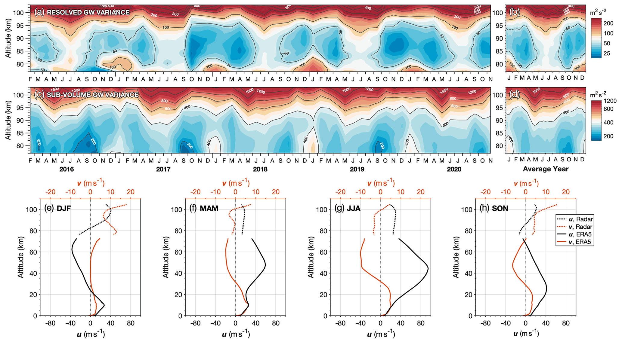
Figure 7 Wind variance against height due to gravity waves (GWs) for (a, b) large-scale “resolved” GWs in the derived winds and (b, c) small-scale “sub-volume” GWs. Panels (e)–(h) show seasonal averages of zonal u (black, lower axis) and meridional v (orange, upper axis) winds against height from ERA5 reanalysis (solid) and the meteor radar (dotted) over South Georgia for the period 2016 to 2020.

Climatological zonal (black, bottom axis) and meridional (orange, top axis) wind speeds against height are shown in panels (e)–(h) for four seasons during 2016 to 2020 from ERA5 (Copernicus Climate Change Service, 2017) reanalysis produced at the European Centre for Medium Range Weather Forecasts (ECMWF). ERA5 winds are averaged over a horizontal region 400 km radius from the island for each height level to simulate the radar's field of view. Winds in the MLT from the South Georgia radar for the same time periods are shown by the dotted lines.

Both GW variance methods exhibit annual and semiannual cycles in Fig. 7. Above 90 km altitude, a large wintertime maximum is observed and a smaller maximum is found during summer, with local minima near the spring and autumn equinoxes. At altitudes below 90 km, there is a summertime maximum with smaller values near the spring and autumn equinoxes in September and March and a weaker maximum during mid winter. These seasonal patterns are consistent with those of previous studies of high latitude GW variance in the MLT (Mitchell and Beldon, 2009; Song et al., 2021), but to our knowledge this is the first time these two GW variance methods have been compared using measurements from the same radar.

One interesting result is how closely the resolved GW variance follows a seasonal cycle, with a clear symmetry around the winter solstice in Fig. 7b. This is encouraging considering that the method is sensitive to only a small range of GW periods 2≲τ≲6 h. The summertime maximum in the resolved variance is also proportionally larger than the equivalent summertime maximum in the sub-volume variance, suggesting a significant role for large-scale internal GWs in the MLT in summer.

The result that both methods exhibit similar seasonal activity suggests that GWs at a wide range of GW scales broadly follow the same seasonal pattern in the MLT at this location. There does not appear to be a significant period where one method shows large variance but the other does not, suggesting that the sources and filtering of these waves could follow similar patterns. It could also be the case that the small-scale GWs in the sub-volume method could be secondary GWs (2GWs) generated in situ from the breaking or dissipation of the larger-scale GWs in the resolved method, as discussed by Vadas and Becker (2018). Although the modelling study of Becker and Vadas (2018) predicted scales of several hundreds of kilometres for these 2GWs, the recent studies of Lund et al. (2020) and Fritts et al. (2021) used a higher spatial resolution localised model over the southern Andes to suggest that 2GWs at much smaller scales of less than 100 km could be generated. Note that GW-breaking, large-scale turbulence and secondary GW generation are all expected to be detectable in the simple GW variance, not just propagating GWs. Further exploration of this topic is needed to constrain the origins of the GW variance in radar observations over South Georgia, such as the inclusion of coincident nadir sounding satellite observations (e.g. Kogure et al., 2020).

Regarding GW directions, we can infer that, by considering the summertime zonal wind profile in Fig. 7e, the measured GW variance in the mesosphere over South Georgia during summer is likely to be due to GWs with eastward (positive) phase speeds that can propagate freely upwards to the MLT without breaking at critical levels where the wind speed equals the phase speed. These GWs are likely to be of non-orographic origin, considering the eastward winds near the surface. GWs westward (negative) phase speeds with sources in the troposphere, such as orographic “mountain” waves, are unlikely to reach the mesosphere during summer due to critical filtering by westward winds in the stratosphere and above.

Conversely, GW variance in the MLT during winter is not expected to be due to GWs with eastward phase speeds propagating up from near the surface due to the strong filtering effect of the eastward zonal winds below (Fig. 7g). Despite this, as discussed by Becker (2012), the thermal structure of the MLT at polar and high midlatitudes exhibits a residual circulation that is likely indicative of an eastward momentum forcing due to GWs. They proposed that this issue can be explained by the impact of 2GWs generated in the breaking regions of orographic “primary” GWs with westward phase speeds. The significance of this is discussed further in Sects. 8 and 9 below.

8 Comparison of radar winds and satellite temperatures with WACCM

In this section, we compare the observed winds from the South Georgia meteor radar and temperature measurements from MLS to climatological winds and temperatures in WACCM. WACCM is a comprehensive global climate model that extends from near the surface to the lower thermosphere, at around 140 km altitude. As global-scale numerical climate models are being cautiously extended into the mesosphere and lower thermosphere, meteor radar measurements of wind remain one of the only continuous long-term wind measurement techniques that can be used to constrain circulations and guide future development of these models. As discussed in Sect. 2.3, the WACCM simulations cover the period 1950 to 2014 and were prepared for the CMIP6 model intercomparison project.

Here we show the WACCM monthly-mean zonal and meridional winds and temperatures against height interpolated to the location of South Georgia. The selected run used an ensemble of three realisations from which we take the ensemble mean. We take a climatological average of WACCM monthly mean winds and temperatures for all years during 2000 to 2014 inclusive. This time period was carefully selected to be long enough for any oscillations near 11 years (e.g. solar cycle) to average out, but not so long that any changes due to long-term climate indices (e.g. CO₂) could have an impact (Ramesh et al., 2020). WACCM monthly mean winds and temperatures in the MLT for this time period were carefully inspected (see Fig. S3), and interannual variability (such as the magnitude and sign of the zonal winds in winter or the height of the summertime zonal wind reversal) was found to be relatively small (that is, a few kilometres or a few metres per second. Therefore, we can have good confidence that a meaningful comparison can be made between the climatological average of WACCM winds and temperatures for 2000 to 2014 and an average of meteor radar winds and MLS-derived temperatures over South Georgia for 2016 to 2020.

8.1 Comparison of zonal and meridional winds

Figure 8 shows average years of monthly mean meteor radar, WACCM, and MLS winds and temperatures over South Georgia from 60 to 105 km altitude. The MLS temperatures are averaged over a horizontal area less than 400 km radius from the island for each height level to simulate the radar's field of view. In panels (b), (d), and (f), tick marks on the right hand axis indicate the approximate altitudes of the WACCM vertical grid levels.

Figure 8 Comparison of an average year of meteor radar-derived zonal (a, b) and meridional (c, d) winds and satellite-derived temperature measurements from MLS (e, f) in the mesosphere and lower thermosphere with climatological winds and temperatures from WACCM simulations over South Georgia.

During summer, both the radar and WACCM exhibit a realistic zonal wind reversal from westward to eastward in the MLT. However, the wind reversal in WACCM occurs at around 75 km altitude compared with around 85 km in the radar observations, and the magnitude of the summertime eastward jet is around 20 m s⁻¹ larger in WACCM. Further, the duration of these summertime conditions is shorter than observations indicate, lasting from only November to February in WACCM but from October to March in the radar. Another interesting point is that, below 90 km altitude, the observed zonal wind in the MLT at high midlatitudes typically exhibits a rapid reversal from eastward to westward at the onset of spring followed by a slowly descending reversal with height back to eastward throughout summer into autumn (e.g. Fritts et al., 2010b; Sandford et al., 2010; Stober et al., 2021c). The zonal winds in WACCM do not appear to follow this characteristic structure in the wind reversal, instead showing a relatively smooth and equal transition in and out of summertime conditions.

The most significant difference, however, between the radar observations and WACCM in Fig. 8 is the direction of the wintertime zonal winds. Radar and satellite observations indicate that the wintertime winds are eastward throughout the MLT at high midlatitudes during winter, forming part of a mesospheric extension of the eastward stratospheric polar vortex (e.g. Beldon and Mitchell, 2009; Harvey et al., 2019). In WACCM, the zonal winds decelerate and eventually reverse to westward above 85 km altitude throughout April to September. This was the case in every year of the WACCM run during 2000 to 2014 (see Fig. S3) and is also the case for the 1850 to 2014 mean, as shown by Ramesh et al. (2020). This difference is well known (e.g. Smith, 2012; Harvey et al., 2019) and may be considered one of the most significant biases in numerical simulations of the MLT, with important impacts for MLT chemistry. There is a growing body of literature that suggests that this reversal of the modelled zonal winds could be due to an incomplete representation of drag due to GWs, in particular, 2GWs (Vadas and Becker, 2018; Becker and Vadas, 2018; Vadas et al., 2018; Heale et al., 2020, 2022). This aspect is discussed further in Sect. 9.

In the meridional direction, the magnitude and altitude of the largest northward winds during summer shows good agreement between WACCM and the radar, reaching maxima of around 14 m s⁻¹ between 75 and 80 km.

However, in the radar observations, this summertime flow remains northward and extends to 105 km altitude, but in WACCM it weakens and reverses to southward above 90 km altitude during November to February. This southward flow in WACCM is part of a summertime winter-to-summer pole flow in the lower thermosphere discussed by, for example, Liu (2007) and Qian et al. (2017), that occurs at higher altitudes (above around 100 km) than the well-known summer-to-winter pole circulation in the MLT region.

Our radar observations, however, do not show evidence of this flow in the height range considered here and are consistent with other meteor radar observations sites around the world, as shown recently in the study by Stober et al. (2021c). Of the six radar sites considered by Stober et al., including four high-latitude locations in Argentina, Antarctica, and Scandinavia, none showed a significant summertime meridional wind reversal from equatorward to poleward flow between altitudes of 80–100 km, as predicted by the WACCM simulation used here. Observations from the powerful SAAMER radar system at Rio Grande, the closest radar site to South Georgia, extend to 110 km altitude but do not show a meridional wind reversal either. Further, meridional wind observations from an equatorial meteor radar site on Ascension Island do not show a reversal between 82 and 95 km, as shown in the study by Davis et al. (2013). These results suggest that the summertime winter-to-summer flow simulated in WACCM is likely to occur at altitudes well above around 105 to 110 km in the real atmosphere.

During winter, meridional flow in the radar observations in Fig. 8c is southward at around 2 to 10 m s⁻¹ below 100 km altitude, above which there is a weak reversal to northward up to 10 m s⁻¹. In WACCM, this reversal appears to occur nearly 20 km lower at around 80 km altitude. There is also an interesting feature of a brief reversal from southward to northward in the radar winds during midwinter (around June–July) that is found to occur in 3 of the 5 years in the radar observations (see Fig. 4) but is not seen in any year in WACCM during 2000 to 2014 (see Fig. S3). As discussed in Sect. 4 above, this could also be due to quasi-stationary PWs, which can introduce an apparent bias into the observed MLT winds when only a single location is considered, such as here over South Georgia. Meridional winds in WACCM in Fig. 8d, however, do not show features to suggest that any such planetary waves might have similar effects in the model.

8.2 Comparison of temperatures in the MLT

Temperatures from MLS and WACCM are shown in Fig. 8e, f. The temperature structure of the MLT is one of the primary drivers of the residual circulation that we observe in our mean wind measurements from the radar (Becker, 2012; Smith, 2012). As both winds and temperatures affect wave propagation and dissipation, realistic simulations of both are necessary to adequately represent the interactive dynamics.

The seasonal cycle is characterised by a cold summertime mesospause below 160 K and a warmer wintertime upper mesosphere of more than 200 K. The seasonal temperature variability in panels (e) and (f) of Fig. 8 closely corresponds to the wind patterns seen in panels (a) to (d). In WACCM, the summertime mesopause is approximately the same temperature as that observed by MLS, but it is tightly located to between 75 and 80 km altitude, which closely corresponds to the strong zonal wind gradient with height in panel (b) and the largest northward winds in panel (d). Conversely, the observed MLS temperature structure during summer has the same summertime mesopause temperatures below 160 K, but it is centred at around 15 km higher in altitude and spread over a larger vertical region. This corresponds to a large vertical spread in the northward meridional wind in the radar in panel (c) and a smaller zonal wind gradient with height in panel (a). As discussed above, the summertime temperature conditions in WACCM do not start as early or persist as long as the observations suggest. Cold polar mesopause temperatures have a first- order effect on the formation of polar mesospheric clouds, which are involved in the annual creation and destruction of key chemical species. An improvement in simulating these cold polar temperatures is therefore likely to lead to improved long-term forecasts of atmospheric chemistry at climate timescales in WACCM simulations that include these chemical processes.

During winter, the mesopause occurs at approximately the same altitude in both MLS and WACCM, but in WACCM it is around 20 K warmer. This could be indicative of an anomalous westward GW drag in the polar region in WACCM that causes an anomalous polar warming (Becker, 2012), driving a westward vertical shear of the residual wind with increasing altitude, which eventually reverses, as shown in Fig. 8b. Further, a strong positive temperature gradient above the mesopause in WACCM indicates a faster transition into the thermosphere than observed by MLS throughout the year. This aspect could help to explain the reversal of the summertime meridional winds in WACCM from northward to southward above 90 km altitude and the lower vertical extent of northward winds during winter.

9 Discussion

9.1 Secondary GWs and differences between radar observations and WACCM

In Sect. 8 we highlighted several differences between the observed and simulated temperature structures and residual circulations in radar and satellite observations and WACCM. One key discrepancy is westward winds during winter in WACCM that are not observed by the radar.

Unlike the lower atmosphere, the temperature structure and residual circulation of the MLT region is highly sensitive to the drag and driving effects of atmospheric waves, particularly GWs (e.g. Smith, 2012; Becker, 2012). In global models, however, parameterisations must be used to account for GW processes due to their relatively small size (particularly near their sources) compared with the model grid (Holton, 1983; McLandress and Scinocca, 2005). The GW parameterisation in WACCM uses a discrete spectrum of GWs and is based on the approach of Lindzen (1981), with several updates (Richter et al., 2010; Garcia et al., 2017).

Westward wintertime winds in the simulated polar MLT are a long-standing feature of WACCM (Harvey et al., 2019; Ramesh et al., 2020; Stober et al., 2021c), but they are also found in the thermospheric extension WACCM-X (Liu et al., 2010; Pedatella et al., 2014; Liu et al., 2018; Pancheva et al., 2020) and in other high-top models such as the MUAM (Lilienthal et al., 2018). Although not all global model configurations yield this feature, models that do simulate the observed eastward winds in winter may each have other biases of their own in other altitude regions, as shown by Pedatella et al. (2014) and more recently by Stober et al. (2021c). Careful tuning of the GW parameterisation scheme in WACCM may likely produce a closer agreement to the observations for a given season; however, this may give rise to other biases in different regions and seasons.

The long-standing nature of this discrepancy is indicative of the complexity of the processes involved, and likely the importance of accurately simulating the momentum deposition effects of GWs.

Although authors suggest impacts of secondary GWs as a promising mechanism to improve the MLT simulations of whole atmosphere models based on recent studies (e.g. Becker and Vadas, 2018), there are also substantial uncertainties regarding impacts of GW generation due to flow imbalance in the upper stratosphere and lower mesosphere.

As discussed by Becker and Vadas (2018) and Vadas and Becker (2019), it has been proposed that at high latitudes during winter, primary GWs propagate upwards from near the surface and undergo wave breaking and/or diffusion, which provides a local body force on the background flow. These local body forces then act to generate 2GWs, which they themselves break and generate tertiary waves, and so on. This multi-step vertical coupling changes the direction of the momentum deposition in the MLT, as secondary waves are generated in concentric rings in all directions except for perpendicular to the direction of the initial primary wave (Vadas et al., 2018; Lund et al., 2020; Kogure et al., 2020; Fritts et al., 2021; Heale et al., 2022). This anomalous eastward drag causes and anomalous cooling over the polar cap, which results in an eastward wind shear with altitude in the residual circulation of the MLT, as observed by the KEP radar in Fig. 8. It should also be mentioned that there is substantial additional uncertainty surrounding GWs generated due to flow imbalance in the upper stratosphere and lower mesosphere itself, a process that is also not included in standard model parameterisations. The impact of these additional non-orographic primary GWs on the MLT region is still not fully understood.

These issues mean that even if the filtering of surface-launched parameterised GWs by the background winds is correctly specified in model parameterisations, and the columnar assumption of vertical wave propagation is reasonably valid, it is the final step of directional GW momentum deposition (either by primary or by secondary GWs) that must be accurately simulated to develop realistic circulations in the MLT. The proposal of Vadas and Becker (2018) and Becker and Vadas (2018) is to resolve these 2GWs through the accurate simulation of local body forces on the atmosphere during wave breaking and dissipation, which then spontaneously generate propagating 2GWs. Another approach could be to develop a multi-height GW drag parameterisation scheme (e.g. Ribstein et al., 2022) which may be computationally cheaper to implement.

9.2 On the directional separation of sub-volume GW variance

In Sect. 7 we used the simple method of Mitchell and Beldon (2009) to derive estimates of sub-volume GW variances from meteor radar observations over South Georgia. In the initial submission of this paper (available online), we went further to explore the separation of this sub-volume GW variance into different directions, namely the variance of GW perturbations in the east–west (zonal) and north–south (meridional) directions. Given a long enough time window for sufficient meteor echoes (we used a rolling monthly window), this can be done by binning (or weighting) the residual velocity perturbations by azimuth to obtain an estimate of the directional orientation of the measured GW variances. The initial results yielded an apparent seasonal cycle in the directionality of the sub-volume GW variance.

However, we include an important note here regarding one problem with this method. The problem derives from the error in the height determination of meteor echoes and the subtraction of the local background wind to yield residual wind perturbations (which are assumed to be due to GWs). If the background wind conditions were always uniform with height, the method would work perfectly despite this error. However, during summer there is a strong zonal wind shear located near the meteor echo detection peak between 85 and 90 km altitude (see Fig. 4). This significant change in the zonal wind speed with altitude means that errors in the meteor echo height determination could lead to significant inaccuracy in the subtraction of the local background wind component. This would lead to increased variance in the residual wind perturbations during summer, especially when considering only the zonal direction, which could be incorrectly attributed to increased variance due to zonally orientated GWs. This is what was observed in the initial submission of this paper, but we are unable to separate variance because of this effect of genuine changes in GW variances in different directions. We therefore include this note as a caution until a method is developed that can separate variance in the zonal direction due to these two effects during summer with confidence.

10 Summary and Conclusions

In this paper we have described a new SKiYMET meteor radar system deployed at King Edward Point on South Georgia island (54^∘ S, 34^∘ W). The radar system made near-continuous measurements of winds in the mesosphere and lower thermosphere from February 2016 until it was removed in November 2020. Here, we described a new Gaussian weighting method for improved time–height resolution of meteor radar winds, characterised the mean winds, solar tides, PWs, and GWs in the MLT over South Georgia and compared our measurements with a climatological WACCM simulation from the CMIP6 project. We find that:

1. The large-scale zonal winds in the MLT above South Georgia are characterised by eastward flow up to 40 m s⁻¹ during winter and a zonal wind shear from around 20 m s⁻¹ westward to 40 m s⁻¹ eastward during summer. The large-scale meridional winds are characterised by poleward flow during winter below 100 km and equatorward flow during summer from 75 to 105 km altitude.

2. The semidiurnal solar tide is dominant at this latitude, reaching up to 80 m s⁻¹ during April and May and exhibiting a clear annual and semiannual cycle. The terdiurnal and quardiurnal tides are also found to maximise during May with amplitudes of more than 10 and 5 m s⁻¹ respectively, whereas the diurnal tide is comparatively weak (around 10 m s⁻¹) at this latitude, especially during winter.

3. The Q2DW in the MLT reached very large amplitudes of more than 30 m s⁻¹ in the meridional direction during January 2019. We also measure zonal amplitudes of up to 15 m s⁻¹ at PW periods near 5, 6, 10, and 16 d during winter and, by combining our measurements with those from the nearby SAAMER meteor radar at Rio Grande, we find that these PWs have predominantly westward propagating modes 1 and 2.

4. The variance of wind perturbations due to both large-scale “resolved” GWs and small-scale “sub-volume” GWs exhibit similar annual and semiannual cycles throughout the MLT. Comparatively larger variance is due to large-scale GWs during summer, which we propose corresponds to eastward propagating non-orographic waves from below.

5. The climatological WACCM simulation exhibits a summertime mesopause that is up to 10 K warmer and ∼ 10 km lower in altitude than observed by the South Georgia radar and by MLS, above which simulated eastward zonal winds are up to 20 ms larger than observed. Simulated summertime meridional winds also reverse to poleward above 95 km, implying a winter-to-summer pole circulation in the lower thermosphere in WACCM that is not found in this altitude range in our radar observations.

6. Most significantly, the observed wintertime zonal winds throughout the MLT are eastward up to 40 m s⁻¹ but in the WACCM simulation they are westward up to 20 m s⁻¹ above 80 km altitude. This coincides with a wintertime mesospause in WACCM that is nearly 20 K warmer than that observed by MLS. We propose that this large discrepancy could be due to the impact of an anomalous eastward forcing by secondary GWs that is not currently simulated in WACCM, leading to an unrealistic thermal structure and residual circulation.

These results highlight the important contribution that measurements of the MLT made at remote locations such as South Georgia can provide to develop our understanding of MLT wind, wave, and tidal dynamics. These insights can be used to constrain and guide the development of general circulation models as they are extended into this dynamic region of the earth's atmosphere.