the Creative Commons Attribution 4.0 License.
the Creative Commons Attribution 4.0 License.
 | 20 Jul 2022
Radiative closure and cloud effects on the radiation budget based on satellite and shipborne observations during the Arctic summer research cruise, PS106
Carola Barrientos-Velasco
Hartwig Deneke
Anja Hünerbein
Hannes J. Griesche
Patric Seifert
Andreas Macke
For understanding Arctic climate change, it is critical to quantify and address uncertainties in climate data records on clouds and radiative fluxes derived from long-term passive satellite observations. A unique set of observations collected during the PS106 expedition of the research vessel Polarstern (28 May to 16 July 2017) by the OCEANET facility, is exploited here for this purpose and compared with the CERES SYN1deg ed. 4.1 satellite remote-sensing products. Mean cloud fraction (CF) of 86.7 % for CERES SYN1deg and 76.1 % for OCEANET were found for the entire cruise. The difference of CF between both data sets is due to different spatial resolution and momentary data gaps, which are a result of technical limitations of the set of shipborne instruments. A comparison of radiative fluxes during clear-sky (CS) conditions enables radiative closure (RC) for CERES SYN1deg products by means of independent radiative transfer simulations. Several challenges were encountered to accurately represent clouds in radiative transfer under cloudy conditions, especially for ice-containing clouds and low-level stratus (LLS) clouds. During LLS conditions, the OCEANET retrievals were particularly compromised by the altitude detection limit of 155 m of the cloud radar. Radiative fluxes from CERES SYN1deg show a good agreement with ship observations, having a bias (standard deviation) of −6.0 (14.6) and 23.1 (59.3) W m−2 for the downward longwave (LWD) and shortwave (SWD) fluxes, respectively. Based on CERES SYN1deg products, mean values of the radiation budget and the cloud radiative effect (CRE) were determined for the PS106 cruise track and the central Arctic region (70–90∘ N). For the period of study, the results indicate a strong influence of the SW flux in the radiation budget, which is reduced by clouds leading to a net surface CRE of −8.8 and −9.3 W m−2 along the PS106 cruise and for the entire Arctic, respectively. The similarity of local and regional CRE supports the consideration that the PS106 cloud observations can be representative of Arctic cloudiness during early summer.
- Article
(6741 KB) - Full-text XML
- BibTeX
- EndNote


Arctic warming is a robust feature of climate change (Meredith et al., 2019). The Arctic air temperature increases at more than twice the rate of the global mean air temperature (Ballinger et al., 2020). This phenomenon, named Arctic amplification, has been predicted by models and confirmed by measurements (Serreze and Barry, 2011; Winton, 2006; Johannessen et al., 2004). Clouds strongly influence the atmospheric energy budget and are a primary source of uncertainty in the Arctic climate system (Huang et al., 2017; Tan and Storelvmo, 2019; Zib et al., 2012).
Arctic clouds are complex due to their complicated structure, complex interactions with various physical processes, and feedbacks (Morrison et al., 2012; Kay et al., 2016). They influence the shortwave (SW) and longwave (LW) fluxes, thereby modulating the radiation and heat budgets. In the summer Arctic, the highly reflective surface and low sun angles enhance cloud-surface reflections (Curry et al., 1996; Barrientos Velasco et al., 2020). Therefore, an effective combination of observations and modelling is needed to better understand Arctic clouds and climate (Kay et al., 2016).
A key advantage of using satellite instruments for investigating changes in the climate system, is the provision of consistent observations covering relatively long time periods with near-global spatial coverage (Stubenrauch et al., 2013; Christensen et al., 2016; Huang et al., 2017). For example, Hartmann and Ceppi (2014) find large changes in the Arctic radiation budget at the top of the atmosphere (TOA), based on CERES (Clouds and the Earth's Radiant Energy System) observations, with trends of −5 and 3 W m−2 per decade for the SW and LW net fluxes, respectively. In contrast, Devasthale et al. (2016) report large discrepancies and no significant trends in cloud data records based on the Advanced Very-High-Resolution Radiometer (AVHRR). Hence, these observations require critical evaluation to identify their shortcomings before they can be used to diagnose processes responsible for Arctic climate change.
Due to the limited availability of ground-based observations in the Arctic, only a few studies have compared ground- and satellite-based observations of clouds and radiative fluxes. Dong et al. (2016) present a radiative closure (RC) study comparing ground-based and satellite retrievals of microphysical and radiative properties of single-layer clouds at the Atmospheric Radiation Measurement North Slope of Alaska (ARM NSA) site at Utqiaġvik, Alaska. Considering overpasses of the Terra and Aqua satellites from 2000 to 2006, and the CERES Synoptic 1∘ daily flux (SYN1deg, eds. 2 and 4) products (Loeb et al., 2009; Rutan et al., 2015; Minnis et al., 2020), this study reports good agreement of retrievals of liquid water path (QL) and cloud optical depth (τ) under both snow-covered and snow-free surface conditions. Using ARM and CERES SYN1deg cloud retrievals as input for radiative transfer simulations, the modelled downward SW fluxes (SWD) agree with the corresponding ARM observations and CERES SYN1deg products within 10 W m−2.
The investigation by Riihelä et al. (2017) presents an intercomparison between ground-based observations and several satellite products of surface (SFC) radiative fluxes. Downward and upward LW and SW radiative flux observations, from the Tara drifting ice camp and long-term observations on the Greenland Ice Sheet, are compared to the CERES SYN1deg ed.3A, FluxNet, and Satellite Application Facility on Climate Monitoring cLoud, Albedo and RAdiation (CLARA) data sets (Karlsson et al., 2017), and the Global Energy and Water Exchanges (GEWEX) Surface Radiation Budget (SRB; (Wu and Fu, 2011)). This study concludes that CERES SYN1deg has the smallest root-mean-square error (RMSE) compared to in situ fluxes. This study recommends further investigation of differences in the surface and cloud properties that lead to discrepancies in flux retrievals.
Alongside RC studies with satellite products, ground-based long-term observations can provide independent estimates of the cloud radiative effect (CRE), and thus show how clouds influence the radiation budget. For example, Ebell et al. (2020) simulated radiative fluxes based on more than 2 years (June 2016 to September 2018) of cloud properties retrieved from remote-sensing observations with the Cloudnet algorithms at the atmospheric observatory of the Arctic French–German research station – The German Alfred Wegener Institute for Polar and Marine Research and French Polar Institute Paul Emile Victor (AWIPEV) – at Ny-Ålesund, Norway (Nomokonova et al., 2019). Simulated and observed surface broadband LW and SW fluxes were compared for all-sky (AS), clear-sky (CS), and cloudy conditions. For AS conditions, a mean difference of 3.1 and 0.2 W m−2 was found for the SWD flux and the downward LW (LWD) flux, respectively, confirming RC for the study period. Based on the simulations, estimates of CRE at the SFC (CRESFC), TOA (CRETOA), and within the atmosphere (CREATM) were derived. For the location of Ny-Ålesund, the annual averages revealed a surface warming by clouds of about 11.1 and −16.1 W m−2 at the TOA, with significant variability observed particularly during summer.
In contrast to large-scale observations, field campaigns provide a higher degree of detail to investigate relevant physical processes, and to study remote locations with previously poor observational coverage. The Surface Heat Budget of the Arctic Ocean (SHEBA) programme investigated the physical processes governing the surface energy budget and sea-ice mass balance, covering the Beaufort Sea and a complete annual cycle from October 1997 to October 1998 (Uttal et al., 2002). Based on SHEBA data, Shupe and Intrieri (2004) determined the CRESFC, considering the influence of surface albedo (α) and cloud properties in detail. This study found that low-level liquid clouds had the largest radiative effect. This study also recommended the use of polarization-sensitive lidars to improve the differentiation of ice crystals and cloud droplets, and to generally improve retrieval algorithms for estimating liquid water content (qL) towards a better understanding of the radiative effect of Arctic clouds.
With the aim to better understand the physical mechanisms underlying Arctic Amplification, the project Arctic Amplification: Climate Relevant Atmospheric and SurfaCe Processes and Feedback Mechanisms (AC)3 held two major field campaigns in the early summer of 2017, northwest of Svalbard (Wendisch et al., 2019). Both campaigns performed in situ and remote-sensing observations over the Arctic Ocean. While ACLOUD (Arctic Cloud Observations Using Airborne Measurements during Polar Day) was an aircraft campaign, the PS106 shipborne campaign took place aboard the German research vessel (R/V) Polarstern. The PS106 expedition consisted of two legs, PASCAL (Physical Feedbacks of Arctic Boundary Layer, Sea Ice, Cloud, and Aerosol; PS106/1) from 24 May to 21 June 2017, and with some observations continuing during SiPCA (Survival of Polar Cod in a Changing Arctic Ocean; PS106/2) from 23 June to 20 July (Macke and Flores, 2018). The mobile remote-sensing platform OCEANET-Atmosphere (hereafter denoted as OCEANET) was set up aboard Polarstern (Macke, 2009; Kalisch and Macke, 2012; Hanschmann et al., 2012; Kanitz et al., 2013; Griesche et al., 2020). The atmospheric observations collected with OCEANET were subsequently utilized to derive macro- and microphysical properties of clouds based on the Cloudnet algorithm (Illingworth et al., 2007; Griesche et al., 2020).
The present paper aims to investigate the radiative effects of clouds and their influence on the radiation budget during the PS106 expedition. Radiative fluxes are simulated based on reanalysis profiles and observed cloud properties. They are compared to the CERES SYN1deg ed. 4.1 products (hereafter referred to as CERES SYN1deg), as well as shipborne flux observations as a basis for a radiative closure assessment. From these data, an estimate of CRE and the radiation budget during PS106 is given. Our investigation specifically attempts to answer the following questions:
-
How consistent are cloud properties derived from the ship-based observations and the CERES SYN1deg cloud products?
-
How closely do our radiative transfer simulations agree with the CERES SYN1deg SFC fluxes and Polarstern flux observations under CS conditions?
-
Under which circumstances is it possible to confirm RC between flux observations, our radiative transfer simulations, and the CERES SYN1deg products?
-
What was the radiation budget during PS106, how was it influenced by clouds as quantified by CRE, and how representative were the local conditions for the entire Arctic?
The paper is structured as follows: first, Sect. 2 presents a description of the observations and methods. Results and discussion follow this description in Sect. 3. Its first part summarizes the atmospheric conditions during PS106, followed by a sensitivity study to determine the uncertainties of the radiative transfer simulations. The differences between simulations and observations are quantified for specific case studies, and the entire PS106 expedition is discussed in Sect. 3.3. and 3.4, respectively. Based on these results, Sect. 3.5 presents the estimated radiation budget and CRE for PS106 and the entire Arctic. Finally, the paper closes with conclusions and an outlook to future research in Sect. 4.
This section describes the shipborne observations and resulting cloud products, as well as the satellite-based cloud and radiation products used as basis for this study. Furthermore, a description of ancillary data, used for the radiative transfer simulations and to describe the surface and atmospheric conditions, are presented alongside the method used for the radiative transfer simulations. In addition, a classification of sky conditions based on the shipborne data sets and the setup used for the broadband radiative transfer simulations are introduced.
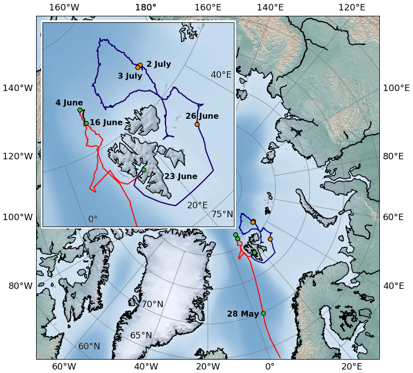
Figure 1Cruise track of the Polarstern PS106 expedition is shown on a polar stereographic map of the Arctic. The red line shows the track for the first leg (PS106/1, also denoted as PASCAL), the black line indicates the position for the ice floe camp during PASCAL, and the blue line shows the cruise track for the second leg (PS106/2, also denoted as SiPCA). The upper left box zooms in the ice floe camp drift. Green dots indicate the start of the PASCAL and SiPCA legs, and the beginning and end of the ice floe camp. Orange dots depict the location of several case studies.
2.1 Shipborne data set
2.1.1 Shipborne instrumentation
The OCEANET facility was established to provide continuous atmospheric observations aboard research vessels such as the German icebreaker Polarstern. It has been operated since 2009 during transfer cruises between the hemispheres, crossing the Atlantic Ocean from Bremerhaven in Germany, to Punta Arena in Chile, and Stellenbosch or Cape Town in South Africa (Macke, 2009; Kalisch and Macke, 2012; Hanschmann et al., 2012; Kanitz et al., 2013). In 2017, OCEANET was operated for the first time in the Arctic Ocean during two legs of the PS106 expedition named PASCAL and SiPCA, respectively (see Fig. 1; Macke and Flores, 2018; Griesche et al., 2020).
The instrumentation of OCEANET consists of a multiwavelength Raman polarization lidar, PollyXT, a 14-channel microwave radiometer (MWR), a Humidity And Temperature PROfiler (HATPRO), and a fish-eye sky camera. For the first time in the standard OCEANET observations, a Doppler cloud radar of type Mira-35 was installed about 10 m above the container during the PS106 cruise, complementing the OCEANET observations. The cloud radar can profile optically thick clouds and measure Doppler spectra produced by the vertical cloud motion due to its polarimetric capabilities, and valuable information on the hydrometeor type can also be derived. These remote-sensing instruments are combined with observations by an optical disdrometer of type OM470, and Vaisala RS92-SGP radiosondes launched every 6 h as input to the Cloudnet processing (see Sect. 2.1.2; Griesche et al., 2020).
On the roof of the measurement container, a CMP21 broadband pyranometer (0.285–2.8 µm) and a CGR4 broadband pyrgeometer (4.5–42 µm), both manufactured by Kipp & Zonen, were installed. For surface radiation measurements in polar regions, the accuracy of these instruments is expected to be within ±10 and ±20 W m−2 for pyrgeometers and pyranometers, respectively (Lanconelli et al., 2011). In the case of the pyrgeometer, additional uncertainties due to variation in the vertically integrated water vapour (IWV) column need to be considered. At values below 10 mm of IWV, the atmospheric window produces spectral inhomogeneities, which distort the pyrgeometer measurements (Gröbner et al., 2014). Gröbner and Wacker (2015) compared the performance of a calibrated World Infrared Standard Group (WISG) and a CGR4 pyrgeometer, and found that for specific periods, deviations can reach up to ±3 W m−2. Thus, in this study, the total instrumental uncertainty for the pyrgeometer is assumed to be ±13 W m−2. Operating these instruments aboard Polarstern might introduce additional uncertainties due to harsh environmental conditions like the exhaust plume of the ship, and the superstructures of the ship interfering with the observations (see Fig. A1).

Figure 2Time series of surface properties along the PS106 cruise track. Panel (a) shows the surface albedo based on CERES SYN1deg in red. Panel (b) shows the temperature based on Polarstern (PS) observations at 10 m a.s.l. in orange, and the skin temperatures from ERA5 and CERES SYN1deg in blue and red, respectively. The lower coloured band indicates the times when Polarstern was located in open ocean (blue), the marginal sea-ice zone (yellow), and in mostly sea ice (teal).
In addition, a meteorological station measuring atmospheric pressure, temperature, and relative humidity with a sensor of type Series EE33 from E+E Elektronik, was installed at about 10 m above sea level (m a.s.l.) next to the OCEANET container during PS106. The measured values of this near-surface temperature are presented in Fig. 2b.
2.1.2 Cloudnet products and description of sky conditions
The Cloudnet project targets a systematic evaluation of the representation of clouds in the weather forecast and climate models (Illingworth et al., 2007). Within its scope, a robust suite of algorithms has been developed for retrieving vertical profiles of macro- and microphysical properties of clouds from a synergistic combination of cloud radar, lidar, and MWR observations. A complete description is given in Illingworth et al. (2007), while details about its adaptation for PS106, including a new approach for the continuous determination of the ice effective radius (rE,I), is presented in Griesche et al. (2020). This section provides a summary of the Cloudnet products used as the basis of the present study, i.e. the location of the cloud boundaries, as well as vertical profiles of qL, liquid effective radius (rE,L), ice water content (qI) and rE,I.
As a first step, the measurements are averaged onto a common pixel grid with a vertical and temporal resolution of 31.18 m and 30 s, respectively, leaving a total of 595 vertical pixel grids and, in general, more than 2700 time steps (Griesche et al., 2020). Then, each pixel is categorized into seven distinct classes, following a bitwise diagnosis described by Hogan and Connor (2004). The final target classification provides 11 different pixel categories: clear sky, cloud droplets only, drizzle or rain, drizzle or rain and cloud droplets, ice, ice and supercooled droplets, melting ice, melting ice and cloud droplets, aerosols, insects, and aerosols and insects.
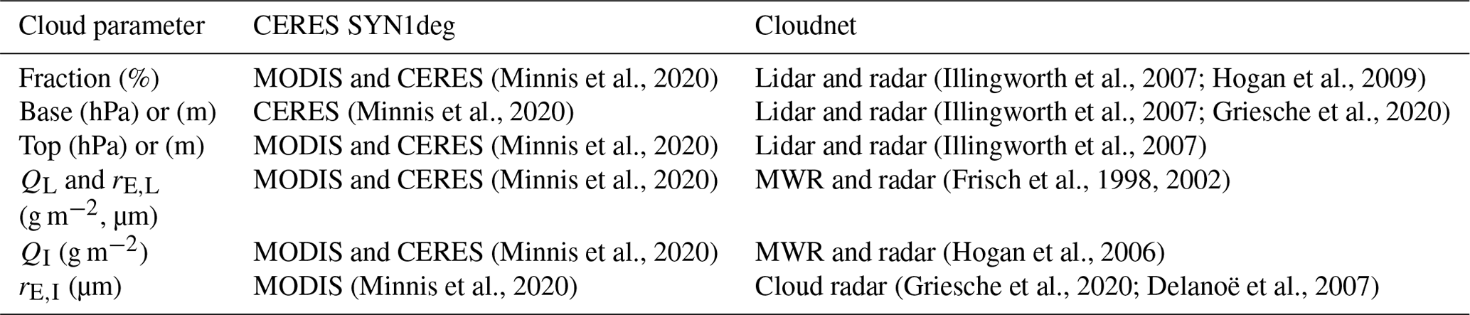
(Minnis et al., 2020)(Illingworth et al., 2007; Hogan et al., 2009)(Minnis et al., 2020)(Illingworth et al., 2007; Griesche et al., 2020)(Minnis et al., 2020)(Illingworth et al., 2007)(Minnis et al., 2020)(Frisch et al., 1998, 2002)(Minnis et al., 2020)(Hogan et al., 2006)(Minnis et al., 2020)(Griesche et al., 2020; Delanoë et al., 2007)Table 1Table indicating references and remote-sensing instrumentation used to derive cloud macro- and microphysical properties for CERES SYN1deg and Cloudnet data sets. Units are shown in brackets.
The determination of the cloud thermodynamic phase is implemented following the methodology introduced in Griesche et al. (2020), which is based on the lidar and radar measurements (see Table 1). The liquid phase is assigned to pixels when the lidar backscatter signal exceeds a threshold of Mm−1 sr−1, and is reduced by at least a factor of 10 within 250 m due to the strong attenuation by liquid clouds. When the Doppler radar signal indicates falling particles at a dew point temperature below 0 ∘C, the pixel is considered as ice. If both criteria are fulfilled simultaneously, the pixel is classified as a mixed-phase pixel.
Once a cloudy pixel is identified, the cloud water content and effective radius are determined, regardless of whether the cloud is detected as a single or mixed-phase cloud. The QL is retrieved based on the HATPRO MWR measurements using the retrieval method developed in Löhnert and Crewell (2003). This method relies on a long-term radiosonde training data set, which in this case is based on Ny-Ålesund, NO (78.9∘ N, 11.85∘ E, WMO Code 6260). Once QL is known, qL and rE,L are determined. The retrieval of qL is obtained by distributing the observed QL from the HATPRO MWR adiabatically among the identified liquid and mixed-phase cloud pixels classified by the Cloudnet algorithm. This method assumes a log-normal cloud-droplet size distribution, which is constant with height. The uncertainties of qL are calculated by error propagation assuming a typical uncertainty of 20–25 g m−2 in QL (Löhnert and Crewell, 2003). The retrieval of rE,L considers the radar reflectivity factor and the profile of QL based on the methodology described in Frisch et al. (2002). The reflectivity used to derive the rE,L was likely not affected by the presence of ice crystals, since most of the mixed-phase cloud cases observed during PS106 had cloud top temperatures larger than −10 ∘C and a radar reflectivity around −20 dBZ (not shown). The study of Bühl et al. (2016) showed that at these temperatures and radar reflectivities, the signal of the mixed-phase cloud is dominated by the presence of liquid droplets rather than the ice crystals. In cases where the radar reflectivity is lower (e.g. −40 dBZ) the ice crystals dominate the signal of the mixed-phase cloud more, and other methods are necessary to derive the rE,L (Kalesse et al., 2019; Radenz et al., 2019).
The qI is obtained based on the measurements from the cloud radar for pixels flagged as ice or mixed-phase cloud (Hogan et al., 2006). The ice water path (QI) is calculated by vertically integrating qI. These parameters depend on temperature (T; ∘C) and cloud radar reflectivity (Ze; dBZ). Based on the values of qL and qI, vertical profiles of cloud fraction (CF) are calculated. The rE,I is derived based on empirical relationships between the visible extinction coefficient, cloud radar reflectivity and model temperature, as it is further described in Griesche et al. (2020). Additionally, Cloudnet provides CF, averaged to hourly values for 67 equidistant height layers, with a thickness of 300 m, ranging from 150 m up to 19.95 km (see Fig. 4a).
The Cloudnet products also contain quality flags that indicate when the pixels have a reliable retrieval, contain a mixture of liquid droplets and ice crystals, and when large ice crystals, drizzle, or rain might bias the radar reflectivity. Precipitation (PPT) conditions compromise the retrieval accuracy of QL and QI from the MWR and cloud radar, respectively.
Three independent types of flagging categories are used to complement the analysis. These flags are based on Cloudnet target classification, and the identification of low-level stratus (LLS) clouds from Griesche et al. (2020). Quality flags determine the atmospheric conditions directly affecting the lidar beam or cloud radar signal. This characterization identifies “optimum conditions (OC)”, moments with “LLS clouds”, “PPT”, and “PPT and LLS”. A second classification describes structural flags by identifying “clear-sky”, “single-layer”, and “multilayer” clouds. Moreover, the last flag classification focuses on the cloud phase. We identify “clear-sky” moments, clouds with “PPT”, “ice”, “liquid”, “mixed-phase clouds type 1” in which ice and liquid droplets are separately identified, and “mixed-phase clouds type 2” in which Cloudnet distinguishes a mixed layer of ice and supercooled droplets in the same layer of cloud. Complex cloud systems like multilayer mixed-phase clouds can also be identified by the simultaneous use of structural and phase flags; however, they are outside the analysis of the time series classification (Fig. 5).
The three classification types only focus on clear or cloudy pixels. Thus, as a first step, any Cloudnet pixel of “aerosols”, “insects”, and “aerosols and insects” is removed by changing its assigned value to zero to discard them from the analysis. Once this step is done, a set of iterative conditional assignments is applied independently to each vertical column. For instance, if no cloudy pixel is present in the atmospheric column, that column is flagged as ”clear-sky”. If cloudy pixels are found in a single column, and no clear-sky pixels are identified in between, then the algorithm classifies the column as “single-layer”. If one or more clear pixels are identified between cloudy pixels, the flag of multiple levels is assigned. A similar method is followed, but with different conditions for quality and phase flags. Lastly, the three types of flags are linearly interpolated to match the temporal resolution of the simulations, and stored separately in the output files of the radiative transfer simulations. Section 3.1 provides a broader description of the atmospheric conditions and analysis of the flagging system during PS106.
2.2 Satellite data set
The CERES SYN1deg product provides global SW and LW radiative fluxes at the TOA, at four pressure levels, and at the SFC interpolated to an hourly resolution. While TOA fluxes are directly based on observations by the CERES SYN1deg instruments, in-atmosphere and SFC fluxes are calculated based on the Fu–Liou radiative transfer model (Fu and Liou, 1992), and are adjusted for consistency with the TOA observations (Gupta et al., 2010; Rose et al., 2013; Rutan et al., 2015; Kato et al., 2018; Minnis et al., 2020). The CERES SYN1deg uses cloud properties from geostationary and polar satellites observations, in particular from the Moderate Resolution Imaging Spectroradiometer (MODIS). As ancillary input, CERES SYN1deg relies on reanalysis data from the Global Modelling Assimilation Office's (GMAO) Global Earth Observing System version 5.4 (GEOS-5). In addition to radiative fluxes, various surface, cloud and aerosol parameters are included in the product to enable an exploration of the relationships among clouds, aerosols, and radiation (Minnis et al., 2020). Specifically, CERES SYN1deg provides several relevant cloud properties. The parameters considered in this study are CF, QL, QI, rE,L, rE,I, cloud base (PB) and top pressure (PT). The cloud properties are reported for four atmospheric pressures intervals. Nevertheless, it has been decided to consider the total atmospheric values for the analysis. Note that the cloud properties mentioned are retrieved based on MODIS retrievals of cloud emissivity, cloud effective temperature, cloud particle effective radius, and cloud optical thickness. A description of the retrievals is presented in Minnis et al. (2020). A summary of the cloud parameters used in this study is presented in Table 1. The CERES SYN1deg flux products considered in this study provide fluxes based on an AS, cloudy without aerosols (NA), CS, and virtually pristine (P, neither clouds nor aerosols) scenario.
Amongst the surface parameters included in CERES SYN1deg, α, skin temperature (Ts), and snow/ice coverage are relevant for our analysis. In contrast to previous versions, α is determined considering the 1.24 µm channel instead of the 2.13 µm channel over snow surfaces. This change has the advantage of increasing the range of retrievable cloud optical depths over snow-cover areas (Sun-Mack et al., 2006). However, this modification also increases the uncertainty of α due to higher variability in snow albedo and bidirectional reflectance (Minnis et al., 2020). All CERES SYN1deg parameters are provided on a spatial grid with a resolution of 1∘ latitude by 1∘ longitude and at a temporal resolution of 1 h.
2.3 Radiative transfer simulations
The TROPOS Cloud and Aerosol Radiative effect Simulator (henceforward T-CARS) is a Python-based framework to carry out radiative transfer simulations with a particular focus on the investigation of the radiative effects of aerosols and clouds. Parts of this framework have already been applied and described in Barlakas et al. (2020) and Witthuhn et al. (2021). The T-CARS enables the use of various sources for input data, such as atmospheric profiles of trace gases, temperature, humidity, properties of clouds, aerosols, and surface parameters. The present study employs the widely used rapid radiative transfer model (RRTM) for GCM applications (RRTMG; Mlawer et al., 1997; Barker et al., 2003; Clough et al., 2005).
In this study, the daily T-CARS output files have a standard grid that consists of 197 atmospheric levels ranging from the surface up to 20 km height and 1 min temporal resolution. The first 10 km of the atmosphere is divided into 160 levels with a geometric layer thickness of 62.5 m. The level thickness of each pixel for the first 10 km of the atmosphere corresponds to two vertical levels of Cloudnet's pixel which are averaged to the standard grid. The following 5 km of the atmosphere have a layer thickness of 250 m, while the last 5 km of the atmosphere have a layer thickness of 193.8 m.
Hourly pressure level profiles of temperature, pressure, ozone mass mixing ratio, and specific humidity from the European Centre for Medium-Range Weather Forecasts (ECMWF) Re-Analysis (ERA5) data set are used as input parameters for the simulations. The ERA5 uses 4D-Var assimilation using polar and geostationary satellites, surface, radiosonde, dropsonde, and aircraft measurements (Hersbach et al., 2020). In the case of PS106, the Vaisala Radiosonde RS92-SGP launched from Polarstern every 6 h were also assimilated.
The atmospheric temperature and pressure measured at 10 m a.s.l. aboard Polarstern are used in T-CARS as Ts and surface pressure, respectively. We opted for this setup since these parameters are the closest to the surface and are the only measurements available for the entire cruise. For comparison purposes, the surface temperature from ERA5 and CERES SYN1deg are also considered.
The α for the radiative transfer simulations is based on CERES SYN1deg. The data set is interpolated in space and time to the position of Polarstern at 1 min resolution for the entire PS106 cruise.
All input data sets are linearly interpolated to the standard grid. For trace gases, the climatological values from the Air Force Geophysics Laboratory (AFGL) sub-Arctic summer atmosphere (Anderson et al., 1986) are used. The pressure level ERA5 data set is used in the model by interpolating atmospheric pressure, temperature, specific humidity, and ozone mass mixing ratio. Considering the Cloudnet cloud properties, rE,L and rE,I are linearly interpolated onto the standard grid. The values of qL and qI are converted to values of QL and QI by multiplying with the layer thickness.
For the LW and SW simulations, the RRTMG parameterizations for ice and liquid cloud optical properties are based on the radiative transfer model, Streamer, and Key (1996) and Hu and Stamnes (1993), respectively, have been selected. The parameterization for ice clouds assumes spherical ice crystals with rE,I values with an allowed range between 5.0 and 131.0 µm. Radiative fluxes are known to be sensitive to assumptions about the crystal habit, e.g. hexagonal shape (Wendisch et al., 2005). However, the decision was made based on the availability of parameterizations in RRTMG and to be consistent with the Cloudnet parameterization of ice crystals. In the case of rE,L, the model only allows values within the range from 2.5 to 60 µm. To maximize data coverage, the Cloudnet rE,L values below 2.5 µm have been clipped to this range. Note that this modification increases the original values by less than 0.05 % of the number of observations. Therefore, this choice modification does not significantly change the distribution or mean value of rE,L.
The surface input parameters, such as the ship measurement of pressure, temperature, and the albedo from CERES SYN1deg, are also interpolated to 1 min resolution. The surface emissivity is set to a constant value based on the fraction of sea ice in the vicinity of Polarstern, using CERES SYN1deg as source. When the sea-ice fraction exceeds 50 %, a constant surface emissivity of 0.9999 is used, while a value of 0.9907 is used below this threshold. These constant values are based on Wilber et al. (1999).
The T-CARS output provides vertical profiles of broadband upward and downward LW and SW fluxes, and heating rates for cloudy and CS conditions along the PS106 cruise track. Additionally, the geographic coordinates, the quality flags mentioned in Sect. 2.1.2, profiles of temperature and pressure levels, as well as the cloud top and cloud base height obtained from the Cloudnet data set, and the cloud boundaries from the analysis of LLS described in Griesche et al. (2020) are included as output variables.
The present study defines CRE as the difference between the AS and CS net fluxes in W m−2, following, e.g. Mace et al. (2006). The net CRE is obtained as the sum of the CRELW and CRESW components, which are calculated using Eq. (1). In this equation, “x” stands for either LW or SW, and is computed both at the SFC and TOA. Given the net CRESFC and CRETOA, the net CRE throughout the atmosphere (CREATM) is obtained by subtracting of the values at the TOA and SFC.
The main results of the present investigation are described and discussed in this section. First, the atmospheric and surface conditions during PS106 are described in Sect. 3.1. In Sect. 3.2, a sensitivity study of the radiative fluxes in CS conditions is given in order to quantify the expected uncertainty of the radiative transfer simulations, and to quantify the effect of atmospheric and surface variability on fluxes. Section 3.3 presents three case studies, comparing our own radiative transfer simulations based on T-CARS, the CERES SYN1deg-based flux products, and ship-based flux observations. An assessment of RC for the CERES SYN1deg fluxes considering the entire PS106 cruise is given in Sect. 3.4. The radiation budget and its modulation by clouds as quantified by CRE for the PS106 expedition is investigated in Sect. 3.5. Results obtained along the ship track and for the whole Arctic are compared in order to assess the representativeness of the observations conducted during the PS106 expedition.
3.1 Atmospheric and surface conditions
A general description of the meteorological and synoptic conditions during the PASCAL expedition (leg 1 of PS106) has already been given by Knudsen et al. (2018). Here, a complementary and more specific description is provided, focusing in particular on aspects influencing radiative fluxes, in situ observations, and satellite and ancillary data sets required as input for radiative transfer simulations.
Time series of α, near-surface and Ts along the PS106 cruise track are presented in Fig. 2. The track covered open ocean, the marginal ice zone, and ocean covered by dense sea ice. These regions can be differentiated by their α, which has been obtained here from the CERES SYN1deg data set (see Fig. 2a). The retrieval of α used by CERES SYN1deg is described in Minnis et al. (2020) and references therein. Based on the sea-ice concentration, the ERA5 broadband α is calculated as a linear combination of the sea ice and open water contributions. For the considered time period, the sea-ice concentration in ERA5 is based on the corresponding operational product provided by EUMETSAT's Ocean and Sea Ice Satellite Application Facility (OSI SAF; Eastwood et al., 2014) and the Operational Sea surface Temperature and Ice Analysis (OSTIA) data set (Hirahara et al., 2016). For PS106, there is, in general, a relatively good agreement between both α data sets along the cruise track, with a standard deviation of about 0.1. The largest differences occur during the second leg for the period from 25 June to 8 July 2017, when the CERES SYN1deg albedo is systematically higher than the ERA5-based values. Some of the observed differences might be attributed to the different spatial resolutions of the data sets (1∘ for CERES SYN1deg versus 0.25∘ for ERA5). Another potential cause for discrepancies is the omission of the effect of melt ponds in ERA5, which results in a systematic underestimation of the broadband α by ERA5 from June to mid-August, as discussed in Pohl et al. (2020).
The CERES SYN1deg α is used later as input for the radiative transfer simulations. It is based directly on solar reflectance observations, and due to the maturity of CERES SYN1deg products, it is expected to yield accurate results (Rutan et al., 2015). Its use also ensures consistency with the CERES SYN1deg flux products and allows us to better focus on the influence of other parameters. Nevertheless, the large influence of α on the solar radiation budget is investigated and discussed in more detail (see Sect. 3.5).
The Ts and the near-surface air temperature are warmest at the beginning of the expedition when Polarstern was located over open ocean. For the rest of the expedition, the temperatures maintained a relatively steady value near 270 K, except for 8 June and 3 July 2017, when the temperatures dropped to around 266 K. In general, all temperatures presented in Fig. 2b are in good agreement, except for 29, 9–10, 22–23 June, 3–4, and 15 July 2017. Most of these differences might be due to local variability, as there is good agreement of onboard measurements. The largest difference in Ts between CERES SYN1deg and ERA5 is found for 23 June 2017, which was the start of the second leg where Polarstern was located in Svalbard (see Fig. 1). This difference might be due to the challenges posed by a realistic representation of the marginal sea-ice zone.
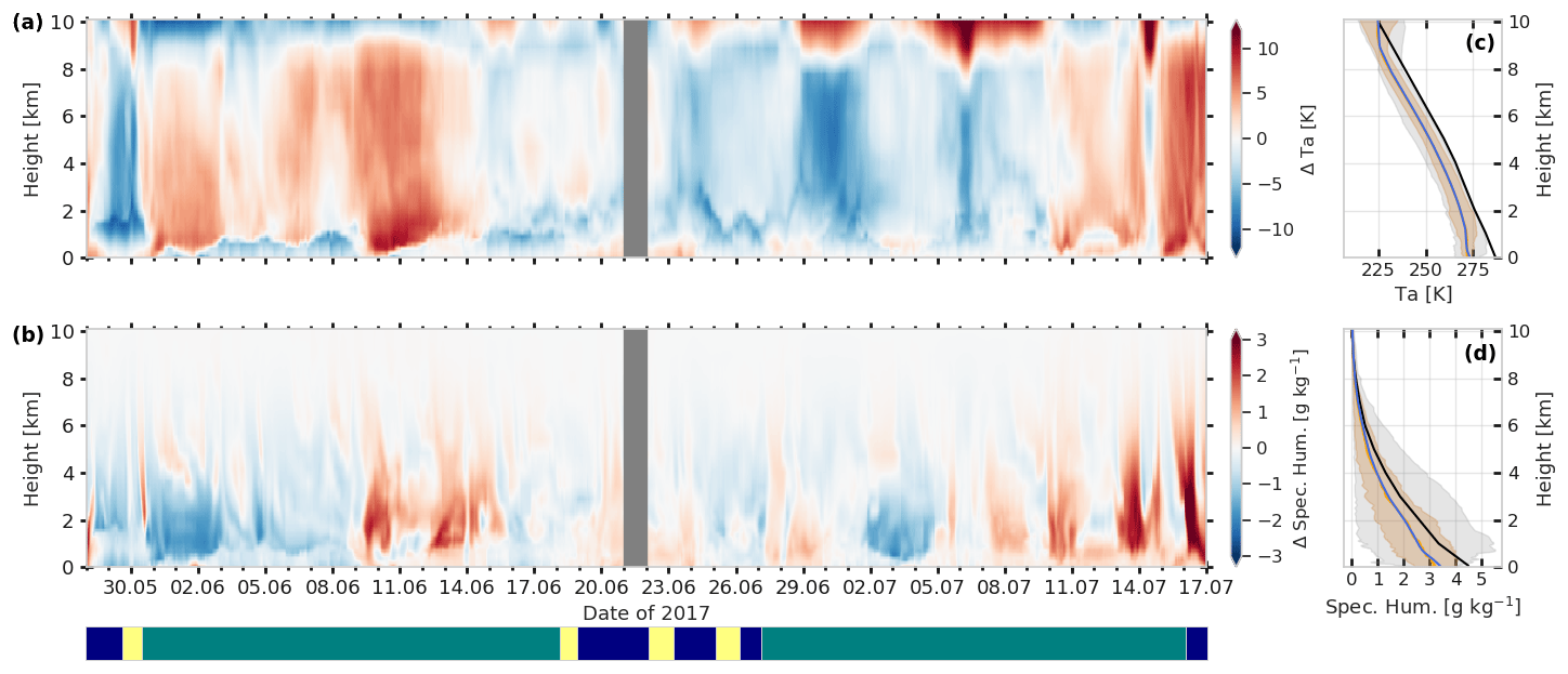
Figure 3Time–height plot of atmospheric profiles obtained along the PS106 cruise track. (a) ERA5 atmospheric temperature anomalies. (b) ERA5 specific humidity anomalies. (c) Mean profiles of atmospheric temperature and (d) mean profiles of specific humidity for ERA5 (orange) and radiosondes (blue). The sub-Arctic summer standard atmosphere (Anderson et al., 1986) is displayed in black. The grey-shaded area indicates the minimum and maximum values, while the brownish-shaded area shows the interquartile range of the ERA5 profiles. The lower coloured band indicates the times when Polarstern was located in open ocean (blue), the marginal sea-ice zone (yellow) and in mostly sea ice (teal).
The anomalies of the vertical profiles of atmospheric temperature and specific humidity based on ERA5 are shown in Fig. 3 for the PS106 track, together with the mean profiles and the sub-Arctic summer standard atmosphere (Anderson et al., 1986). The anomalies have been calculated with respect to the mean profiles of the cruise. Figure 3a and b, indicate a strong temperature and humidity inversion layers from 1–9 June 2017, followed by a generally warmer atmosphere from 10–14 June 2017. Moreover, relatively warm and humid conditions are observed at the end of leg 2 (11–16 July 2017), caused by water vapour transport as described in Knudsen et al. (2018) and Viceto et al. (2022). Based on the shipborne observations, the near-surface temperature varied more strongly during leg 1 than during leg 2 of PS106 (see Fig. 2b). Most of the humidity intrusions observed in Fig. 3b have southerly and westerly origins of the advected air masses, based on the wind direction obtained from the radiosondes (not shown). The mean vertical profiles of atmospheric temperature and specific humidity indicate good agreement of radiosondes and ERA5, which are colder and dryer than the climatological values of the sub-Arctic summer standard atmosphere.

Figure 4Cloud fraction (CF) observed along the PS106 cruise track. Daily mean CF based on Cloudnet plus detection of low-level stratus (LLS) clouds introduced by Griesche et al. (2020) (red) and CERES SYN1deg (blue). The lower coloured band indicates the times when Polarstern was located in open ocean (blue), the marginal sea-ice zone (yellow) and in mostly sea ice (teal).
A characterization of cloud conditions during the PS106 expedition is given next, considering CF, vertical layer structure, and thermodynamic phase. The Cloudnet vertical profiles of CF are shown in Fig. 4a, while a comparison of daily mean CF is presented in Fig. 4b. For the latter panel, Cloudnet and LLS clouds are combined in the comparison to CF values of CERES SYN1deg. All CF values have been aggregated from hourly to daily means. To ensure consistent temporal sampling, hourly values with data gaps in the shipborne observations have been excluded from CERES SYN1deg. It is worth mentioning that the combination of LLS and Cloudnet CF improved the analysis by reducing the fraction of data gaps from 25.2 % to 6.6 % for the entire PS106 period.
The comparison aims to determine the consistency of the CERES SYN1deg and Cloudnet CF, despite their different instrumental origin, perspectives, spatial and temporal sampling, and retrieval algorithms. It is worth noting that CERES SYN1deg provides a spatially averaged CF for a 1∘ latitude by 1∘ longitude region, while Cloudnet yields vertically resolved information on cloud cover as time series for the location of Polarstern. Mean values of CF are 86.7 % and 76.1 % for CERES SYN1deg and Cloudnet plus LLS, respectively. The CERES SYN1deg CF, without exclusion of Cloudnet data gaps, is higher at 86.9 %, indicating that data gaps occur more frequently in cloudy conditions.
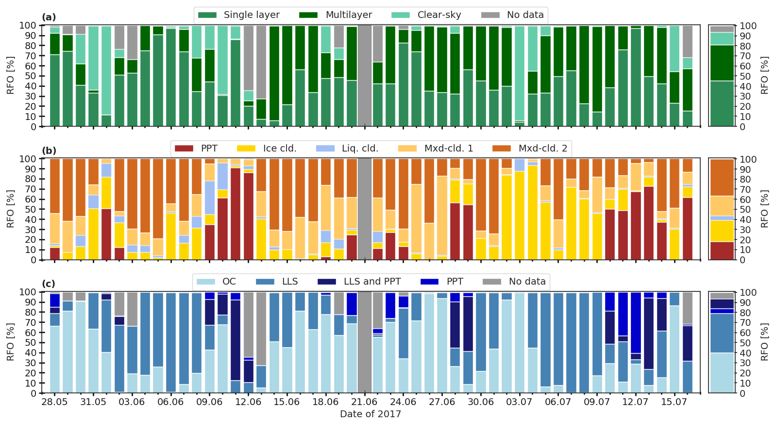
Figure 5Daily and overall relative frequency of occurrence (RFO) of various cloud characteristics. Panel (a) shows the RFO of clear-sky, single-layer clouds, and multilayer clouds. Panel (b) shows the RFO of the thermodynamic phase of single-layer clouds, differentiating periods of ice clouds, liquid clouds, mixed-phase clouds of type 1 or 2, and precipitation (PPT). Panel (c) is the RFO of various quality flags indicating optimum conditions (OC), low-level stratus (LLS), PPT and simultaneous occurrence of LLS and PPT.
A description of the type of clouds observed during PS106 is shown in Fig. 5. The used classification is based on the Cloudnet target classification and supplemented by the analysis of LLS clouds. While the cloud type classification was already presented in Fig. 18c of Griesche et al. (2020), data quality and a more detailed description of mixed-phase clouds are considered here. Details of the classification methodology for the three flags are explained in Sect. 2.1.2.
During PS106, approximately 45.4 % and 35.6 % of the time, single- and multilayer clouds were observed by Cloudnet, respectively (Fig. 5a). The remaining 12.4 % of the time, CS conditions were detected, and data gaps occurred for 6.6 % of the time. While single-layer clouds were more frequent during the first leg, the frequency of multilayer clouds was higher during the second leg (see Figs. 5a and 18c in Griesche et al., 2020). The frequencies of single- and multilayer clouds are typical for early summer conditions, as previously reported by other studies (e.g. Shupe et al., 2011; Nomokonova et al., 2019).
The cloud phase flag was included to analyse the thermodynamic phase of clouds. Even though it is available for the entire PS106 time series, the focus here is directed to the thermodynamic phase of single-layer clouds since these cases are the most frequent, and an analysis is less complex than for multilayer conditions. Figure 5b shows only single-layer cloud periods. This figure indicates an occurrence frequency of 36.7 % for single-layer mixed-phase clouds of type 2 (ice and supercooled droplets), 19.4 % for mixed-phase clouds of type 1 (well-separated ice and liquid phase), and 21.5 % for single-layer ice clouds. The remaining period is composed of single-layer clouds with PPT (17.9 %), and single-layer liquid clouds (4.5 %). We emphasize the need to consider PPT periods since, during these events, there are larger uncertainties in observations (i.e. cloud radar, lidar, MWR, and radiometers).
The quality status flag shows that only 40.1 % of the time, optimum observation conditions were identified (see Fig. 5c). For about 39.0 % of the time, LLS with a cloud base below 155 m prevailed, implying that during these periods, the cloud base height lay below the altitude detection limit of 155 m of the cloud radar (see Fig. 18a in Griesche et al., 2020). The PPT alone, and moments with LLS and PPT occurred for about 5.1 % and 9.2 % of the time, respectively. Under LLS and PPT conditions, the observations of cloud macro- and microphysical parameters have a reduced accuracy. Thus, for only about 40.1 % of the time, observations are of sufficient quality, e.g. for radiative transfer simulations, while observations with a degraded quality occurred for 59.9 % of the period.
3.2 Sensitivity analysis of clear-sky (CS) radiation
This section presents a sensitivity analysis of the radiative fluxes at the surface for CS conditions. Its goal is to quantify the response of radiative fluxes to variability and uncertainty of various atmospheric and surface parameters during PS106, which are required as input to radiative transfer simulations. The accuracy of CS radiative fluxes is of particular interest, as it serves as a reference for the calculation of CRE, and thus places a limit on its accuracy. The propagation of the input uncertainties to radiative fluxes is thus used to establish uncertainty limits for the subsequent RC study.
A CS atmosphere has been created as a reference case, based on the conditions at a position of 81.9∘ N and 32.51∘ E on 3 July 2017. This day was selected because it is the day with the longest CS period during PS106 (see Figs. 1, 4 and 5). For the sensitivity analysis, all atmospheric and surface parameters required as input were prescribed by the actual conditions, with the exception of α, which was kept constant and set to the daily mean value of 0.65. The intention is to avoid resulting variations in fluxes due to fluctuations of the α, which ranged from 0.58 to 0.78 on that day (see Fig. 2a). For the day, the CERES SYN1deg ice coverage lay above 0.5. Thus, the surface emissivity was set to a constant value of 0.9999. The solar zenith angle (SZA) ranged from 59 to 75∘, which does not cover the full range of SZA encountered during the PS106 expedition (47.6 to 80.1∘ for the period from 31 May to 16 July 2017). Despite such minor discrepancies, we assume here that the conditions of this reference day are representative for the entire PS106 cruise for the purpose of this sensitivity analysis.
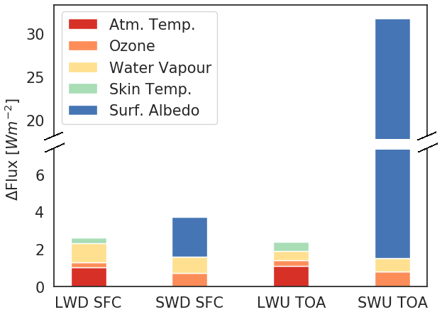
Figure 6Results of the sensitivity analysis visualized as stacked bar chart of the absolute change in CS fluxes in response to perturbations of various input parameters of the T-CARS simulation. Changes are shown for the downward LW (LWD) and SW (SWD) fluxes at the surface (SFC), and the upward LW (LWU) and SW (SWU) fluxes at the top of the atmosphere (TOA), in response to changes in atmospheric temperature, ozone and water vapour column, skin temperature and surface albedo.
The response of radiative fluxes to perturbations of atmospheric parameters, including temperature, ozone, and humidity, has been quantified. In addition, the effects of variations of Ts, α, and surface emissivity are also considered. This analysis focuses on both the downward and upward fluxes at the SFC, as well as the upward fluxes at the TOA for both the LW and SW broadband radiation. A summary of the main sensitivities is presented in Fig. 6, while the full results are listed in the Appendix as Tables A1 to A4. Note that the values used later as uncertainty limits for the RC analysis are highlighted in bold.
The perturbation of atmospheric temperature is based on the instrumental uncertainty of ±0.5 K of the radiosonde temperature sensor, as well as the observed range of atmospheric temperature anomalies of about ±7 K during PS106 (see Fig. 3c). The variation of ±0.5 K has the strongest effect on the LWD flux at the SFC, resulting in a variation of ±1 W m−2. Note that 3 July 2017 is a day with slightly colder than average temperatures for the first 8 km of the atmosphere, and warmer than average temperatures at about 10 km (see Fig. 3a). Considering the larger temperature perturbation of ±7 K results in a variation of up to ±14.9 W m−2 (see Table A1). At the TOA, the variations of ±0.5 and ±7 K yield daily mean differences of ±1.1 and ±15.4 W m−2, respectively.
Ozone reduces the SW flux in the atmosphere by absorption at ultraviolet (λ≲0.35 µm) and visible wavelengths (0.5 µm ≲λ≲0.7 µm). To quantify the sensitivity to ozone, the findings of Bahramvash Shams et al. (2019) are used as basis, who investigated the variation of the vertical profiles of ozone at four Arctic sites from 2005–2017. Perturbation of the ozone column amount by ±12.5 % and ±25 % are assumed. The former value is used to approximate the monthly variation of ozone during summer months (see Fig. 5 in Bahramvash Shams et al., 2019), which is similar to the uncertainty of ±10 % ozonesondes (Deshler et al., 2017). The smaller variation leads to a decrease of ±0.7 and ±0.3 W m−2 at the SFC and TOA for the SW flux, respectively, and ±0.3 W m−2 at both the SFC and TOA for the LW. Variations of ozone concentration are particularly important in the stratosphere, where reduced ozone causes colder temperatures, which enhances the decrease of ozone (Randel and Wu, 1999). It is also worth noting that ozone concentration is linked to synoptic mechanisms through interactions with atmospheric dynamics and photochemistry (Anstey and Shepherd, 2014).
Water vapour is the dominant absorber throughout most of the LW (Delamere et al., 2010) and has strong absorption bands in the SW (λ>900 nm). The strength of SW absorption also depends on the SZA (Wyser et al., 2008). Our sensitivity analysis considers a variation of 5 %, which is used to represent the instrumental uncertainty of radiosondes, and 15 %, which approximates the range between the minimum and maximum column amounts. The variation of 5 % leads to differences of ±1 and ±0.9 W m−2 for the SWD and LWD, respectively, at the SFC. At the TOA, this perturbation yields differences of ±0.5 and ±0.7 W m−2 for the upward LW (LWU) and SW (SWU), respectively (see Table A1). The column amount of water vapour is largest in July, and a positive trend in water vapour since the 1990s has been reported, especially during summer (Di Biagio et al., 2012; Rinke et al., 2019). In addition, recurrent episodes of humidity intrusions can increase the water vapour column by about 8 times above the background level, and increase the LWD flux at the SFC by up to 16 W m−2 (Doyle et al., 2011).
During PS106, the temperature measurement aboard Polarstern closest to the surface was located at 10 m a.s.l. The accuracy of the temperature of ±0.3 ∘C is used for the sensitivity study, together with a perturbation of ±5 ∘C, which corresponds to the largest difference between ship measurements and Ts obtained from ERA5 and CERES SYN1deg (see Fig. 2b). The variation of this parameter only influences the LW fluxes, causing changes of ±0.3 and ±1.4 W m−2 for the LWD and LWU, respectively, at the SFC. At the TOA, a difference of ±0.5 W m−2 is noted in the LWU. Naturally, more considerable variation in Ts yields to larger flux differences as indicated in Tables A2 and A4, which is particularly relevant for days when these differences are more pronounced (e.g. 6–8 June, 22–23 June, 2–5 July 2017; see Fig. 2b).
The α is an extremely important parameter for the SW radiative fluxes (Shupe et al., 2005; Sedlar et al., 2011; Ebell et al., 2020; Stapf et al., 2020). The retrieval of this parameter from satellites in the Arctic is particularly challenging due to the difficulty of cloud detection over snow- and ice-covered surfaces and rapid temporal changes induced by melting. In contrast, ground-based observations often have limited spatial representativeness. Figure 2a shows the time series of hourly α from CERES SYN1deg. From 27 June to 8 July 2017, the difference is most noticeable. For the PS106 cruise, the mean difference of α between CERES SYN1deg and ERA5 is 0.08. For the sensitivity study, the daily mean value of 0.65 is used for α. Variations by ±0.08 are used to investigate the sensitivity of radiative fluxes. Additionally, the minimum (0.05), mean (0.53), and maximum (0.84) values of the CERES SYN1deg α for the entire cruise are used to quantify the sensitivity of SW fluxes to α during the PS106 cruise.
A variation of the α by ±0.08 yields a mean flux difference of ±2.1 and ±33.6 W m−2 at the SFC for SWD and SWU, respectively. This difference also depends strongly on the SZA. For instance, a SZA of 59∘ leads to a flux difference of SWU at the SFC of ±46.6 W m−2, whereas at a SZA of 75∘, this difference is ±20.8 W m−2 (not shown). The values presented in Tables A2 and A4 for the α also indicate the large contrast between the additional values studied (0.84, 0.53, 0.3, and 0.05) minus the constant α of 0.65. At the SFC, open ocean (e.g. α equal to 0.05) causes a large reduction of SWD and SWU by 13.9 and 241.1 W m−2, respectively. On the other hand, the highest α observed during PS106 (0.84) results in an increase of SWD and SWU of 5.1 and 8.4 W m−2, respectively. At the TOA, the daily mean values indicate a reduction by 217.6 and an increase by 72 W m−2 for α of 0.05 and 0.84, respectively. To the best of our knowledge, the importance of α under CS Arctic conditions has also been analysed in other studies (Wyser et al., 2008; Di Biagio et al., 2012; Sedlar and Devasthale, 2012). The values mentioned are consistent with the radiative kernel calculations presented by Bright and O'Halloran (2019) (see their Fig. 1 for the months of June–July–August). Due to the values mentioned, the SWU is the most relevant parameter, sensitive to large differences when estimating the radiation budget and CRE.
The last parameter considered in the analysis is the surface emissivity. A value of 0.9999 is used for surfaces covered by ice, while a value of 0.9907 is used for water surfaces based on Wilber et al. (1999). Additionally, the constant value of 0.988 used by Riihelä et al. (2017) is considered, who used this value for a wider Arctic area, based on Hori et al. (2006). The variation of this parameter only affects the LWU. Contrasting the surface emissivity over sea ice and open ocean, a mean flux difference of 0.8 and 0.7 W m−2 at the SFC and TOA, respectively, are found. The comparison with the value used in Riihelä et al. (2017) yields a smaller difference of 0.2 W m−2 at the SFC and 0.1 W m−2 at TOA.
A summary of the results of the sensitivity study is shown in Fig. 6. Considering the propagation of the uncertainty of input parameters to radiative fluxes, a total uncertainty of the LWD and SWD fluxes at the SFC of ±2.6 and ±3.7 W m−2, respectively, is inferred. The largest part of this uncertainty is introduced by the amount of water vapour and the atmospheric temperature for LWD, and by the α for SWD. Combining these values with the instrumental uncertainties presented in Sect. 2.1.1, total uncertainty limits of ±16 and ±24 W m−2 for LWD and SWD, respectively, at the SFC are inferred as basis of the subsequent RC assessment for CS conditions.
It is worth clarifying that additional uncertainties come from neglecting the presence of aerosols, the assumption of near-surface temperature as Ts, the extrapolation of hourly data to 1 min resolution, the assumption that the coarse spatial grid of 0.25∘ latitude by 0.25∘ longitude (i.e. ERA5 data set) or 1∘ latitude by 1∘ longitude (i.e. CERES SYN1deg products) can capture the atmospheric and surface conditions, and variability experienced during PS106. While it was attempted to quantify some of these uncertainties (e.g. the omission of aerosols in Fig. B1 and Sect. 3.4.1), a careful and more specific analysis will be made by carrying out several sensitivity analyses to quantify these uncertainties considering the observations from the Multidisciplinary drifting Observatory for the Study of Arctic Climate (MOSAiC) expedition (Shupe et al., 2022). Our primary focus will be on the spatiotemporal differences among shipborne, reanalysis, and satellite observations, which we believe are the largest source of uncertainties.
3.2.1 Case studies
The following subsection presents three case studies, which have been selected to cover typical sky conditions during PS106. Radiative fluxes and CRE at the SFC obtained from the T-CARS simulations, CERES SYN1deg products, and the shipborne observations are compared to illustrate periods with a good agreement and larger discrepancies. A day with a long CS period, single-layer, multilayer, and mixed-phase clouds are presented. For the cloud cases, the comparison of fluxes is accompanied by a comparison of cloud properties to investigate their role as a potential source for observed differences in fluxes.
For these cases, it is assessed whether RC can be reached between the shipborne observations on the one hand and the T-CARS simulations and CERES SYN1deg products on the other hand. For CS conditions, the uncertainty limits have been established in Sect. 3.2. In contrast to the RC assessment at the SFC, the lack of independent observations and inputs only allow an assessment of the consistency of fluxes simulated by the T-CARS setup and CERES SYN1deg at the TOA.
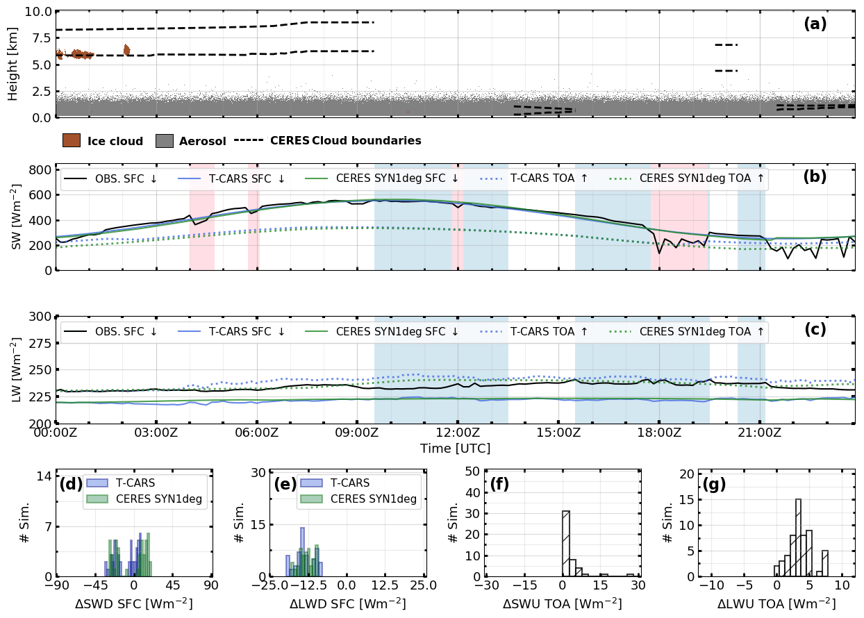
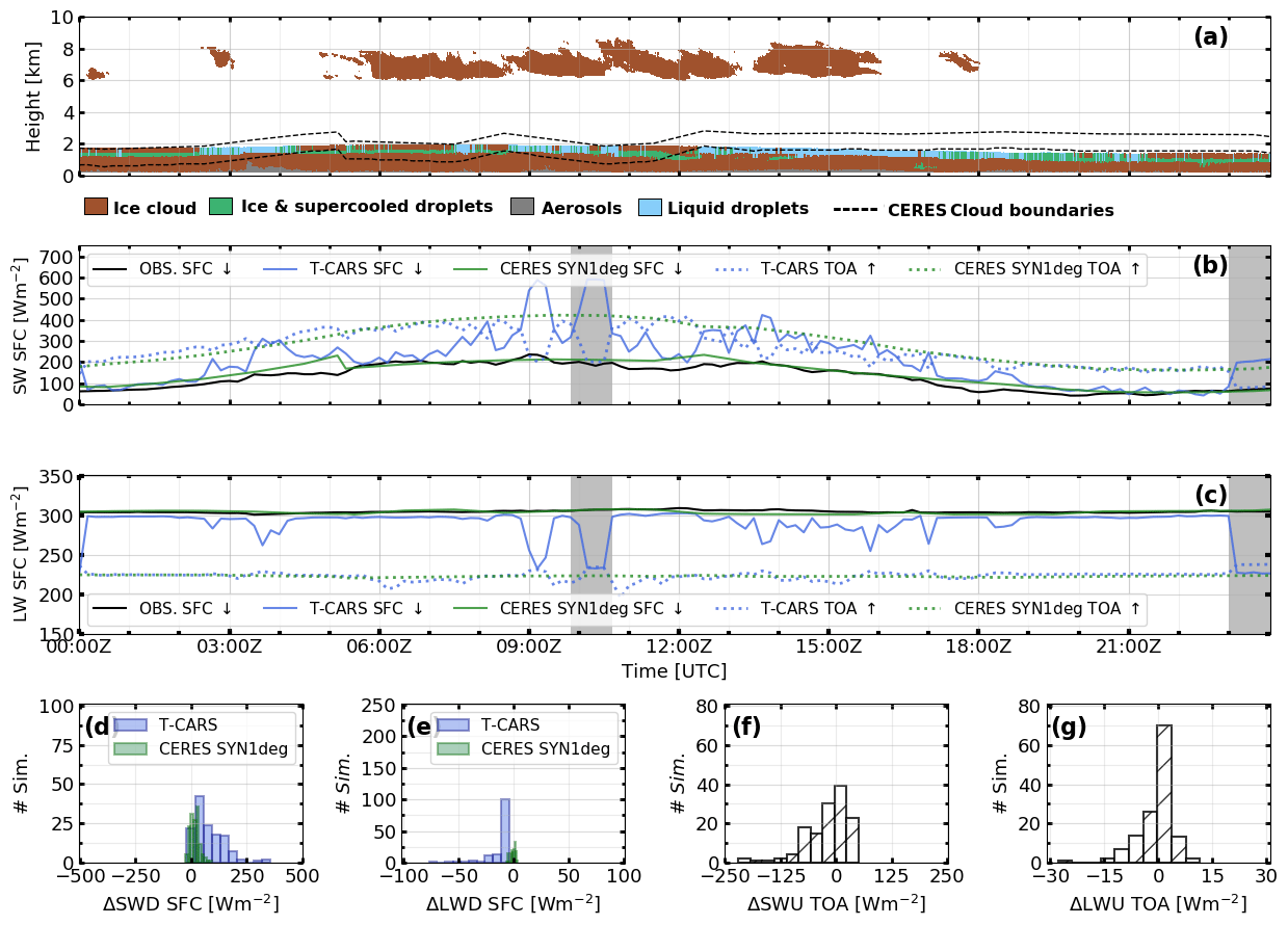
Figure 7Overview of radiative fluxes for the 3 July 2017 case. Panel (a) shows the time series of the Cloudnet target classification and the CERES SYN1deg-based cloud boundaries (dashed black lines). Panel (b) and (c) show the time series of the SW fluxes and LW fluxes, respectively. In both panels (b and c), the down-looking arrow indicates (↓) the downward fluxes at the surface (SFC), and the up-looking arrow (↑) shows the upward fluxes at the top of the atmosphere (TOA). Panels (d) and (e) show histograms of the difference of T-CARS/CERES SYN1deg SWD and LWD fluxes and observations at the SFC, respectively. Panels (f) and (g) show histograms of the difference of T-CARS minus CERES SYN1deg SWU and LWU fluxes at the TOA, respectively. Pink shading indicates periods when the ship's superstructures obstructed the shipborne flux observations. Light-blue background indicates the CS period considered for the analysis.
A common figure layout is used to give an overview of meteorological conditions and radiative fluxes to present the case days in Figs. 7, 8 and 10. Their first panels show the Cloudnet target classification overlaid with the cloud top and base heights obtained from CERES SYN1deg as time series. Panels (b) and (c) show the time series of downward (upward) fluxes at the SFC (TOA) for the SW and LW fluxes averaged to 10 min temporal resolution. Background shading is used for periods when environmental conditions or instrumental limitations compromised the observations. The pink background indicates periods when the shipborne flux observations were obstructed by Polarstern's superstructure, mainly affecting the SW flux. The pale yellow background is used for periods when the Cloudnet retrievals were unable to correct for attenuation, and light blue indicates the periods of CS conditions that are agreeable between CERES SYN1deg and Cloudnet. Panels (d) and (e) show the distribution of the flux difference between shipborne observations and simulations for SWD and LWD, respectively. Panel (f) shows the comparison between CERES SYN1deg products and T-CARS simulations for the SWU flux, panel (g) shows the same as (f), but for the LWU flux.
The comparison of the microphysical properties of clouds such as water path (Q) and effective radius (rE) between Cloudnet and CERES SYN1deg are shown in panels (a) and (b), respectively, of Figs. 9 and 11. Additionally, the time series of CRE at the SFC and TOA based on T-CARS and CERES SYN1deg are presented in panel (c) of the figures mentioned.
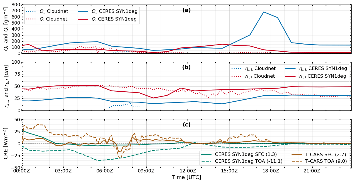
Figure 9Time series of cloud microphysical properties and CRE between CERES SYN1deg and Cloudnet for the 2 July 2017 case. Panel (a) shows the comparison between CERES SYN1deg and Cloudnet of liquid water path (QL; blue) and ice water path (QI; red). Panel (b) shows the liquid effective radii (rE,L; blue) and the ice effective radii (rE,I; red). Panel (c) shows the cloud radiative effect (CRE) at the surface (SFC; solid lines) and the top of the atmosphere (TOA; dashed lines) from T-CARS (brown) and CERES SYN1deg (green).
3.2.2 CS case: 3 July 2017
As mentioned before, 3 July was the day with the longest cloud-free period during PS106 (see Figs. 4, 5, and C1). An overview of meteorological conditions and radiative fluxes for this day is given in Fig. 7. Panel (a) shows that ice clouds were observed by Cloudnet from 00:00 to around 02:30 Z on that day. Later periods when CERES SYN1deg reported clouds while Cloudnet did not, were further analysed by means of the AS camera images. They showed a thin cloud at the horizon for the period between 21:30 to 23:59 Z, which is outside the field of view for the zenith-pointing active remote-sensing instruments.
Good agreement is found for the shipborne flux observations, the T-CARS simulations, and the CERES SYN1deg products for SWD at the SFC. The mean difference of the simulations minus the observations lies below 8 W m−2, a value that is well within the uncertainty limit of ±24 W m−2 used for the RC assessment. For the LWD fluxes, there is a larger difference between the shipborne observations on the one hand, and the T-CARS simulations and CERES SYN1deg products on the other hand. However, the mean difference remains below 14 W m−2, again smaller than the uncertainty limit of ±16 W m−2 chosen for the RC assessment. Therefore, our results confirm that RC is reached for both the SWD and LWD fluxes for this CS case.
To analyse the consistency of T-CARS simulations and CERES SYN1deg products at the TOA, the SWU and LWU fluxes are considered. Figure 7a shows a similar temporal behaviour of the SWU fluxes for the considered period. The mean difference between T-CARS and CERES SYN1deg is 10.0 W m−2, with the largest instantaneous differences occurring after 18:40 Z. Since the T-CARS simulations use the same α as CERES SYN1deg for input, the reason for this difference is most likely due to the spatiotemporal interpolation of CERES SYN1deg (Young et al., 1998). For the LWU fluxes, the mean difference is 3.7 W m−2, possibly due to differences in the CERES SYN1deg Ts and the shipborne measurement of near-surface temperature used by T-CARS (see Fig. 2). The mean differences of the radiative fluxes are sufficiently small to confirm the consistency of CERES SYN1deg and T-CARS fluxes, in agreement with similar studies which compared CERES SYN1deg with other radiative transfer simulations (e.g. Dong et al., 2016; Dolinar et al., 2016).
3.2.3 Single- and multilayer ice cloud case: 2 July 2017
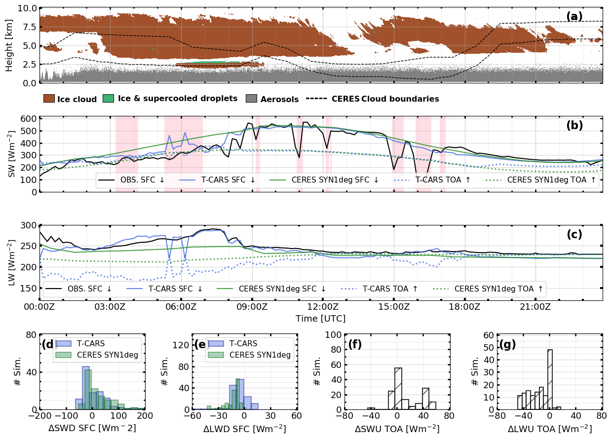
Single- and multilayer clouds were present for 45.4 % and 35.6 % of the time during PS106, respectively (see Fig. 5b). 2 July 2017 has been chosen as the case day with a dominant presence of this type of clouds. Based on the Cloudnet target classification, this day was characterized by well-defined single- and multilayer ice clouds (see Figs. 8a and C2). Middle and high-level ice clouds were observed for most of the day, with an average cloud base at or above 2.6 km. An exception is the period from 05:57 to 08:35 Z, when a relatively thin cloud layer consisting of ice and supercooled droplets was identified (see Fig. 8a). For most of the day, the cloud top height from CERES SYN1deg is significantly lower than that from Cloudnet. The cloud base height is relatively close to the base obtained from the Cloudnet target classification. It is well-known that the retrieval of cloud top height from passive satellite instruments is limited by large uncertainties for thin ice clouds and polar regions (e.g. Yost et al., 2020), so these discrepancies are not surprising.
Table 2Summary of case studies' results. Values indicate the bias and the cloud radiative effect (CRE) for each case study in W m−2 at the surface (SFC) and the top of the atmosphere (TOA).
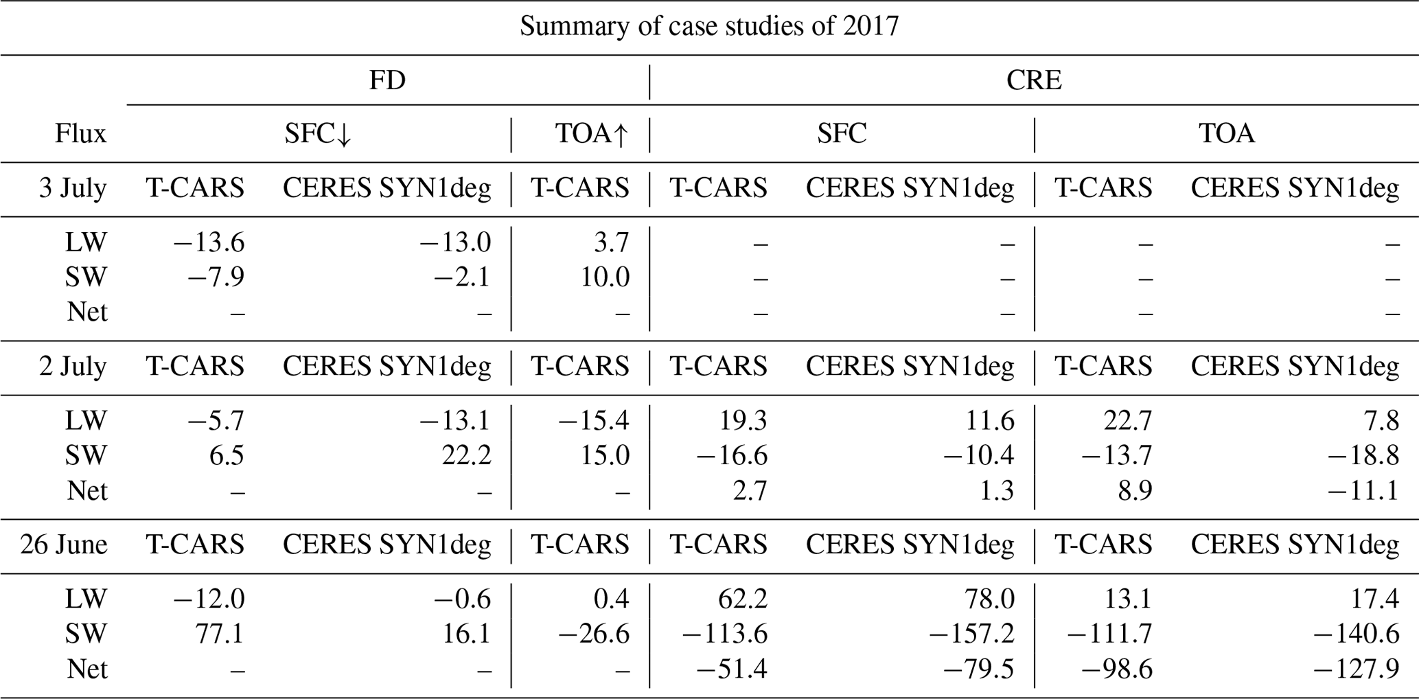
A comparison of CERES SYN1deg and T-CARS fluxes against observations for the SWD and LWD reveals good agreement, with values below the CS uncertainty limits established in Sect. 3.2 (see Table 2). In general, this comparison suggests that RC is achieved for T-CARS and CERES SYN1deg considering the daily mean. At the TOA, however, there is a more significant difference of −15.4 and −15.0 W m−2 for LWU and SWU, respectively. This difference is likely linked to the differences in cloud properties retrieved by Cloudnet and CERES SYN1deg that are displayed in Fig. 9. Discrepancies in other parameters such as the Ts, atmospheric profiles, cloud top height, and cloud geometrical thickness might also be relevant.
Panels (a) and (b) of Fig. 9 show the time series of Q and rE obtained from Cloudnet and CERES SYN1deg, respectively. The comparison of Q shows the integrated values for the entire atmosphere, whereas panel (b) displays the mean values obtained from CERES SYN1deg and the maximum derived by Cloudnet. Despite the difference in retrieval methods, there is, in general, a good agreement between the values of QI and rE,I from CERES SYN1deg and Cloudnet (see Fig. 9a and b). Based on CERES SYN1deg, the entire day was characterized by the presence of a mixed-phase cloud. The values shown for QL are relatively large, especially during the period from 17:00 to 19:00 Z. It is possible that within the CERES SYN1deg footprint, a cloud with such a large QL might have been present. Nevertheless, it is worth noting that the fluxes shown in Fig. 8b and c are calculated considering the CF, which remained below 15 % from 12:30 Z until the end of the day (not shown). The latter suggests that care must be taken when comparing cloud properties obtained from the shipborne active instruments and from CERES SYN1deg with its coarse spatial footprint.
For this case study, the net CRESFC is similar between T-CARS and CERES SYN1deg, despite the noted discrepancies in cloud properties. The net CRESFC has mean values of 1.3 and 2.7 W m−2 for CERES SYN1deg and T-CARS, respectively. At the TOA, the difference is more significant due to the mentioned differences in LW. The net CRETOA derived by T-CARS is 8.9 W m−2, whereas CERES SYN1deg suggests a cooling of −11.1 W m−2. Such inconsistencies need to be clarified and further investigated in future studies.
3.2.4 Mixed-phase clouds: 26 June 2017
The last case study chosen is 26 June 2017. This day was selected due to the presence of well-defined cloud layers consisting of ice and liquid droplets, corresponding to a mixed-phase cloud of type 1. A further reason is the long period of optimum observation conditions reported by Cloudnet (Fig. 5c). Moreover, this day is also of interest due to an underestimation of a high-level cloud amount by CERES SYN1deg in comparison to Cloudnet, as is corroborated in Fig. 10a. This day is also characterized by changing surface conditions, as the ship crossed through the sea-ice transit zone (see Figs. 1, 2a and C3).
This day was characterized by a low-level cloud located within the first 2 km of the atmosphere, and by several periods with a relatively thin ice cloud layer located between 6 and 9 km height (Fig. 10a). According to Cloudnet, the well-separated liquid-phase layer within the ice clouds is characterized by low-radar reflectivity values, upward-directed Doppler velocity, and high-lidar backscatter. There were two moments around 10:00Z and 23:00Z where, due to uncorrected attenuation, QL could not be derived by Cloudnet (Fig. 10a and b). These two moments, marked by the pale-yellow shaded areas, are excluded from the T-CARS and CERES SYN1deg histogram analysis for a fair comparison (Fig. 10d–g).
Panels (b) and (c) of Fig. 10 indicate a good agreement between observations and CERES SYN1deg fluxes. The daily mean difference of fluxes is 16.1 and −0.6 W m−2 for SWD and LWD, respectively. For the T-CARS simulations, the mean flux difference is significantly larger, with 77.1 W m−2 for SWD and −12.0 W m−2 for LWD (see Table 2). Based on these results, RC can be confirmed for the LWD and SWD fluxes from CERES SYN1deg products and the LWD T-CARS simulations. The difference in the T-CARS SWD fluxes exceeds the expected uncertainty limits. To investigate the reasons for this, the cloud properties from both data sets are compared.
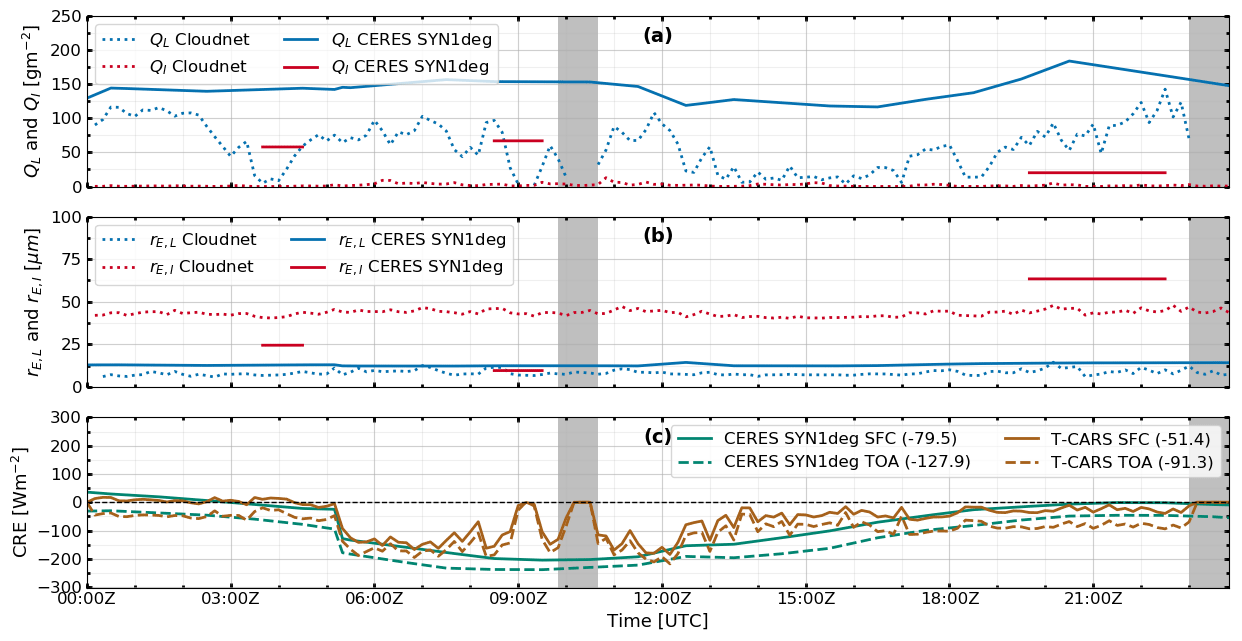
Figure 11Same as Fig. 9, but for the 26 June 2017 case. The grey shading indicates periods with uncorrected attenuation by the Cloudnet products.
Panels (a) and (b) of Fig. 11 show the time series of cloud properties from the Cloudnet and CERES SYN1deg data sets. In contrast to Cloudnet, CERES SYN1deg reports only three periods with the presence of a mixed-phase cloud. The largest difference in cloud properties occurs in the cloud water path products. For Cloudnet, the mean QL is 56.2 g m−2, and for QI, the mean is 1.9 g m−2. In the case of CERES SYN1deg, these values are 119.7 and 38.1 g m−2 for QL and QI, respectively. The variable and lower values of Q are likely responsible for the rapid changes and the positive (negative) bias of the SWD (LWD) flux visible in Fig. 10a and b.
The radiative effect of clouds on this day has a strong cooling influence both at the SFC and TOA, that is enhanced by α. An abrupt change of the CRE at the SFC and TOA is visible at 05:00 Z in Fig. 11c, due to a simultaneous rapid reduction of α from a value of 0.6 to 0.27 (see also Fig. 2a).
Based on CERES SYN1deg, a daily mean net CRE of −79.5 and −127.9 W m−2 is found at the SFC and TOA. The T-CARS simulations also indicate radiative cooling at the SFC and TOA, but smaller in magnitude (see Table 2). As the SWD and LWD fluxes at the SFC from CERES SYN1deg are more consistent with observations, the CERES SYN1deg values are considered to be more accurate.
3.3 Radiative closure assessment based on PS106 observations
In this subsection, CERES SYN1deg fluxes and CS T-CARS simulations are compared to the shipborne observations of the broadband SWD and LWD fluxes for the PS106 expedition. This comparison enables an assessment of RC for the entire expedition, and to identify conditions with significant discrepancies. In Sect. 3.4.1 and 3.4.2, CS and AS conditions are considered separately.
3.3.1 CS radiative fluxes
For the CS comparison, simulated and observed fluxes have been analysed based on the atmospheric classification described in Sect. 3.1 (see Fig. A1). Furthermore, to improve the data quality, AS camera images were used to screen periods with larger differences. With this supplementary information, periods with broken cloud conditions and periods with external factors, which could potentially compromise the radiation observations, were excluded (e.g. the exhaust plume of Polarstern).

Figure 12Histograms of flux difference (FD) of simulations minus observations for the downward LW (LWD) flux (a, c) and the downward SW (SWD) flux (b, d) for clear-sky (CS) conditions. Panels (a) and (b) show T-CARS comparison, where the filled histograms show the filtered data by excluding the moments where the observations were compromised. Panels (c) and (d) show the comparison of CERES SYN1deg for all-sky (AS; green), clear-sky (CS; red) and pristine (P) simulations (blue) for the same filtered time steps as in T-CARS.
The comparison of SWD and LWD fluxes from T-CARS and CERES SYN1deg with shipborne observations for CS conditions is presented in Fig. 12. Figure 12a shows a histogram of the differences of the radiative fluxes from T-CARS minus observations of LWD. This comparison indicates a skewed-left distribution with a negative mean bias of the T-CARS simulations of −24.9 W m−2. After applying the improved quality screening described above, a mean flux difference of −14.2 W m−2 is found, together with a correlation coefficient (R2) of 0.92, and a more symmetric distribution than without this quality screening. The mean flux difference below the uncertainty limit of ±16 W m−2, and the good R2 confirms that RC is achieved for the T-CARS simulations under CS conditions.
In the case of CERES SYN1deg, the mean flux difference between simulations minus observations for the LWD flux is −4.6 W m−2, with a standard deviation of 20.9 W m−2, and a RMSE of 18.5 W m−2. While the bias suggests that RC is found for CERES SYN1deg, the rather low R2 of 0.476 indicates that the values do not reproduce variability as well as the T-CARS simulations, and might be affected by the presence of clouds within the CERES SYN1deg footprint (see Fig. 12c). To test this hypothesis, CS and pristine (P) CERES SYN1deg products were also considered. For both data sets, R2 reached values above 0.765, which confirms that the AS CERES SYN1deg R2 is reduced by the presence of clouds. With this change, the bias however increased to −19.8 and −20.2 W m−2 for the CS and P data sets, respectively (see Fig. 12c).
Several simulations were conducted using only the Vaisala RS92-SGP radiosondes, launched every 6 h from Polarstern (Schmithüsen, 2017a, b), and also sensitivity analyses were made by varying the atmospheric temperature and humidity to try to match the observations of the LWD flux (not shown). However, the negative bias found for both T-CARS and CERES SYN1deg fluxes might also be caused by a positive bias of the shipborne pyrgeometer observations, e.g. due to the influence of the exhaust plume of Polarstern, or other factors affecting the pyrgeometer. As there was only one pyrgeometer measurement aboard Polarstern, it is impossible to further investigate this bias. However, for future campaigns, it is recommended here to operate two pyrgeometers, installed in different locations of the research vessel, to exclude such influences.
The comparison for the SWD flux uses a stricter screening of data, which also excludes all periods when the pyranometer's field of view was obstructed by the superstructure of Polarstern. For T-CARS, a positive bias of 44.2 W m−2 and R2 of 0.85 were found initially, without this screening. With screening, a bias of 9.5 W m−2 and R2 of 0.95 were obtained. In the case of CERES SYN1deg, the biases for AS, CS, and P conditions were found to have values of −27.1, 3.6, and 12.0 W m−2, respectively. These values confirm that the larger negative bias for AS conditions is due to the presence of clouds that were captured within the CERES SYN1deg footprint, but did not pass over the shipborne remote-sensing instrumentation. The second peak, centred around −50.0 W m−2 in Fig. 12d, is most likely due to momentary obstructions on the observations that were not captured by the initial screening that contains about 5 data points of CERES SYN1deg simulations. In general, the biases of T-CARS and CERES SYN1deg are both within the uncertainty limit of ±20 W m−2, indicating that RC is determined for both data sets.
Previous studies reported a similar magnitude of differences between simulated and observed downward fluxes for CS conditions. For instance, the analysis by Ebell et al. (2020) focused on Ny-Ålesund and reported a mean (median) flux difference of −5.0 (−5.5) W m−2 and 12.6 (−2.6) W m−2 for LWD and SWD, accordingly (see their Fig. 3). The studies of Shupe et al. (2015) and Miller et al. (2015) found a median difference of simulations and observations for the LWD (SWD) flux of −6.9 (5.4) and −5.5 (15.6) W m−2 for the Barrow and Summit-Greenland sites, respectively.
The treatment of aerosol in the CERES SYN1deg products is based on the aerosol optical depth (AOD) obtained from the Model of Atmospheric Transport and Chemistry (MATCH; Collins et al., 2001). The comparison between the CERES SYN1deg CS and P fluxes yields a mean difference of 0.4 and −7.5 W m−2 for LWD and SWD, respectively. Considering the entire PS106 cruise, mean flux differences of 0.5 for LWD and −10.8 W m−2 for SWD are found (see Fig. B1a, b, e, and f).
While the LW value indicates that LW aerosol effects are negligible for most purposes, the SW values are relatively large in comparison to the direct aerosol effect of −0.44 to −2.6 W m−2 reported by Rastak et al. (2014).
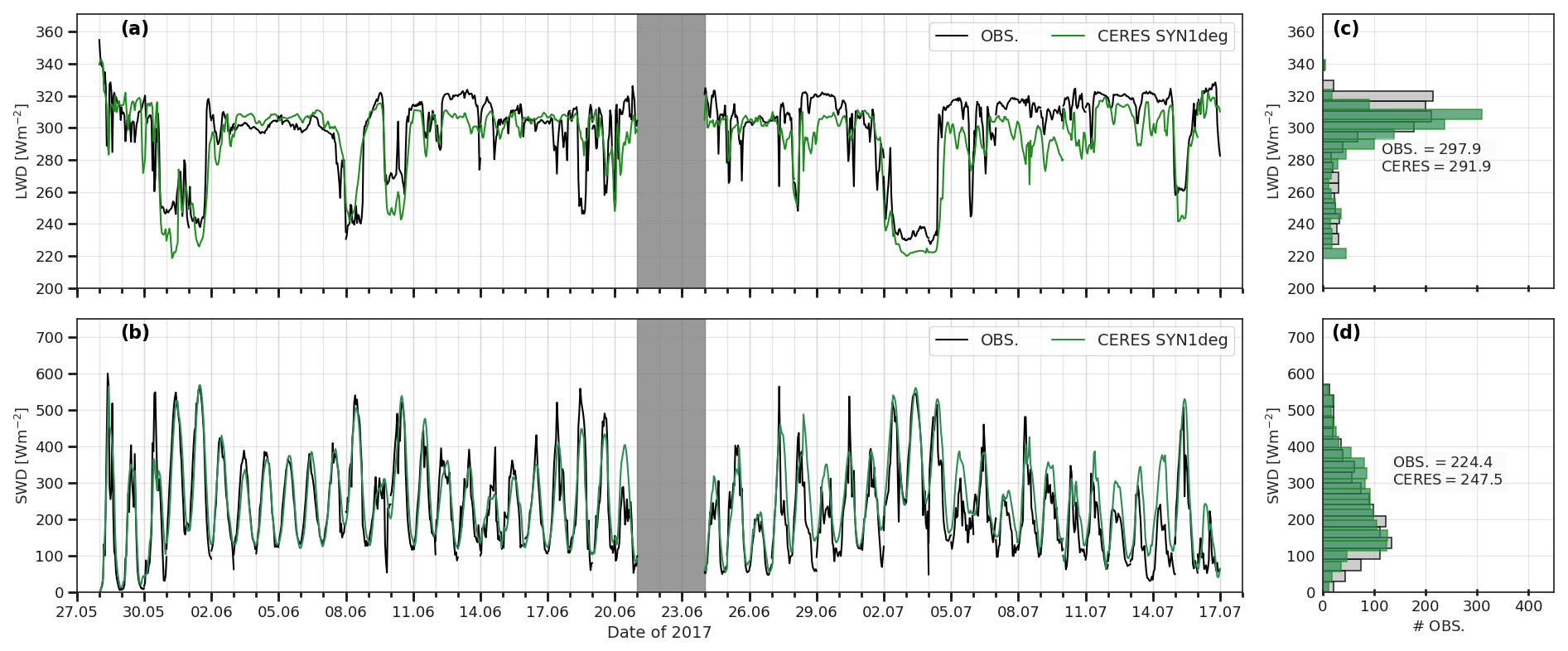
Figure 13Time series during PS106 of downward LW (LWD; panel a) and downward SW (SWD; panel b) fluxes. In panels (a) and (b), observations are shown in solid black lines, CERES SYN1deg AS products in the solid green line. The distribution of each time series is shown in panels (c) and (d).

Figure 14Scatter plots comparing the CERES SYN1deg fluxes and ship-based radiative flux observations (Obs.) for the downward LW (LWD; panel a) and SW (SWD; panel b) fluxes. The black line represents the best linear fit. The resulting fit equation and the square of the Pearson correlation coefficient (R2) are shown in each panel.
3.3.2 AS radiative fluxes
In this subsection, the CERES SYN1deg products are compared to the shipborne observations for AS conditions. The T-CARS simulations analysed as a time series are not considered in the discussion due to the instrumental limitations that occurred during PPT, LLS conditions, or uncorrected attenuation instances, making it impossible to conduct a RC assessment including cloudy-sky conditions. The comparison between observations and CERES SYN1deg fluxes is shown in Figs. 13 and 14. Figure 13a shows the time series of the LWD observations and CERES SYN1deg AS simulations, indicating mostly good agreement. Some periods can be identified with a reduced agreement. These cases occur particularly during PPT periods, which might affect the pyrgeometer measurements (e.g. 12, 20, 28 to 29 June, and 11–14 July). Larger discrepancies are also observed in the presence of multilayer clouds (e.g. 20 June and 5–9 July), which feature a more challenging structure and pose challenges for passive remote sensing (Minnis et al., 2019; Yost et al., 2020).
The discrepancy shown for 13 June 2017 might also be attributed to PPT as it was also the case on 12 June. However, this cannot be confirmed by the observations due to missing data. This day was also brought to attention by Barrientos Velasco et al. (2020), since the near-surface temperature measured on the ice floe by several instruments reached a mean temperature of 281.1, about 4 K warmer than the temperature measured aboard Polarstern (Barrientos Velasco et al., 2020), CERES SYN1deg and ERA5 Ts. This day was also characterized by a more humid than usual upper atmosphere, a cyclonic weather system, northerly winds (Barrientos Velasco et al., 2020), strong temperature inversions, and an intense persistent fog leading to a very low-horizontal visibility (see Fig. 18b in Griesche et al., 2020). This humidity intrusion can lead to an additional energy flux to the surface, enhancing the fog to persist (Tjernström et al., 2019). The fluctuations of atmospheric temperature and relative humidity described might be different from the atmospheric profiles used by CERES SYN1deg, causing the difference of up to 20 W m−2 (Fig. 13a).
The mean flux difference of the LWD fluxes between CERES SYN1deg and observations for AS conditions is −6.0 W m−2, a value that is within the instrumental uncertainty of ±13 W m−2 of the pyrgeometer (see Fig. 13c). Hence, RC for the LWD flux can be confirmed for CERES SYN1deg. Figure 14a shows a scatter plot comparing CERES SYN1deg SFC fluxes with the shipborne observations. The linear regression is calculated and illustrated in the same plot to determine the correlation of both data sets, which indicates R2 of 0.69.
Similar to LWD, there is relatively good agreement between the CERES SYN1deg simulations and observations for SWD for the entire PS106 (see Figs. 13b and 14b). Most of the discrepancies are caused by PPT (e.g. 13 to 14 July), broken cloud conditions, and instances when Polarstern's superstructures compromised the pyranometer observations (see Fig. A1). Figure 13d shows the distribution of the time series of the SWD flux. This panel shows a similar distribution between the observations and the SWD flux simulated by CERES SYN1deg. This comparison indicates that CERES SYN1deg SWD flux is positively biased by 23.1 W m−2, with a standard deviation of 59.3 W m−2. This value is considered acceptable since the instrumental uncertainty is ±20 W m−2, and the moments with broken cloud conditions or obstruction of the observations are not excluded from the comparison. Nevertheless, it is important to stress that obtaining good quality shipborne observations of downward fluxes is challenging due to recurrent obstructions of the view of the radiometer's sensor.
The study of Riihelä et al. (2017) presents a comparison of radiative fluxes between the CERES SYN1deg ed. 3 products and in situ observations from the drifting Tara ice camp from April–September 2007. Their results are presented as daily means and indicate a RMSE of 24.5 and 17.1 W m−2 for SWD and LWD, respectively. In our study, results are relatively similar for LWD, with a RMSE of 12.3 W m−2. In the case of SWD, the RMSE found for PS106 has a value of 46.5 W m−2. It should be noted that our results are based on hourly means instead of the daily mean reported by Riihelä et al. (2017). Furthermore, the observations made during the Tara ice floe camp were unaffected by interference of the ship's superstructure with the observations.
The study by Dong et al. (2016) focuses on the RC of SWD flux for single-layer overcast liquid-phase Arctic stratus clouds over the snow-free and snow-covered surfaces. Their analysis considers CERES SYN1deg eds. 2 and 4 products, which are subsequently compared to radiation observations and cloud retrievals at the ARM NSA site at Utqiaġvik, Alaska. Edition 4 of CERES SYN1deg shows a mean bias against observations below 10 W m−2 for SWD and for snow-free as well as snow conditions. Evidently, our flux difference of 23.1 W m−2 is larger than the value reported by Dong et al. (2016); however, the present study includes more complex cloud situations, which enlarges the differences of radiative fluxes.
3.4 Cloud radiative effect (CRE) and radiation budget during PS106
This section presents an analysis of the radiation budget and CRE for the summertime Arctic and for the period of the PS106 expedition, based on CERES SYN1deg products. While it was initially planned to also include the T-CARS simulations in this analysis, their limited temporal coverage precludes meaningful results. In particular, the exclusion of situations with the prevailing LLS clouds is expected to bias mean fluxes. The CERES SYN1deg data for the period of the first (from 16:45 Z on 28 May until 00:00 Z on 20 June 2017) and second leg of PS106 (22 June to 16 July 2017) are used for consistency with the temporal analyses given in the previous sections. The cruise track during this period lay entirely within the Arctic, defined here to cover the range from 70–90∘ N, and consistent with the definition used by several previous studies (e.g. Walsh et al., 2009; Huang et al., 2017). In addition to the effects of clouds on the radiation budget, the relevance of the direct aerosol radiative effect for the radiation budget is briefly discussed based on CERES SYN1deg data sets.
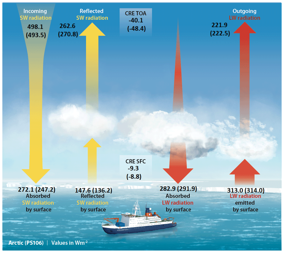
Figure 15Radiation budget for the period of the PS106 cruise. Values show mean values for the Arctic (70 to 90∘ N; top) and PS106 expedition (bottom in parentheses). Shortwave (SW) and longwave (LW) in yellow and red, respectively. Values in central boxes indicate the mean cloud radiative effect (CRE) at the surface (SFC) and the top of the atmosphere (TOA). Period analyzed is from 16:45 Z on 28 May until 00:00 Z on 20 June 2017 and from 22 June to 16 July 2017. Average values are given in W m−2.
An overview of the most important components of the radiation budget is given in Fig. 15, showing mean values along the PS106 cruise track and for the entire Arctic as separate panels. A full list of the different flux components can be found in the Appendix in Table B1. Along the PS106 cruise track and under AS conditions, the radiation budget at the SFC indicates a strong warming influence by the SW net flux with 110.9 W m−2, while the LW fluxes cool the SFC by −22.1 W m−2. The presence of clouds enhances the LWD flux at the SFC by about 62.1 W m−2, while reducing the SWD and SWU by 121.0 and 51.5 W m−2, respectively. For the period of interest, the net radiation budget at the SFC has a value of 88.8 W m−2 for PS106, and a value of 94.4 W m−2 for the entire Arctic. The difference in the net radiation budget for the PS106 track and the entire Arctic is relatively small with a value of 5.6 W m−2, and can be attributed to differences in the mean incoming SW radiation at the TOA, LWD radiation, the transmission of SW radiation through the atmosphere, and α.
At the TOA and for the PS106 cruise, the mean net radiation budget is 0.2 W m−2, while for CS conditions, the net radiation budget would be48.6 W m−2. At the TOA, the presence of clouds increases the reflected solar radiation by 62.9 W m−2 and reduces outgoing LW flux by 14.5 W m−2. For the Arctic, the net radiation budget under AS conditions has a value of 7.8 W m−2, versus a value of 47.9 W m−2 for CS conditions. This indicates that the cooling by CRE is smaller for the entire Arctic than for PS106. This difference can mainly be attributed to an increased reflection of solar radiation due to a larger CF and higher α along the PS106 track compared to the Arctic.
To consider the radiation budget of the atmosphere, the flux divergence has been calculated as the difference of the mean values at the TOA and SFC. The net values found for the entire Arctic (−86.6 W m−2) and PS106 (−88.6 W m−2) show a significant cooling, and are once more relatively similar in magnitude. Since the net radiation budget for PS106 and the Arctic are relatively similar at the SFC, TOA, and within the atmosphere, the PS106 expedition can be considered representative for the entire Arctic (see Table B1).
Additionally, the direct radiative effect of aerosols on the radiative fluxes and the radiation budget has been examined for CS and AS conditions. By considering the different CERES SYN1deg flux products, specifically the AS, cloudy without aerosols (NA), CS, and P fluxes, an estimate of the direct radiative effect of aerosols can be obtained. A summarized version of Table B1 is given in Table B2 in the Appendix, showing the mean perturbation in radiative fluxes arising from aerosols. To be expected, aerosol effects are mainly limited to the SW radiation and are the largest under CS conditions. A decrease of SWD (SWU) of 10.8 W m−2 (6.1 W m−2) is found at the SFC for the PS106 track. Slightly larger values are calculated for the entire Arctic, with a reduction of the SWD (SWU) by 13.9 W m−2 (7.4 W m−2). Aerosols have a small warming effect in LW, leading to an increase no larger than 0.7 and 0.1 W m−2 for LWD and LWU, for both the PS106 track and the entire Arctic, respectively. At the TOA, the effect of aerosols does not surpass more than 0.2 W m−2 for the SWU and LWU fluxes.
Considering net fluxes for P and CS conditions, the direct aerosol radiative effect at the SFC along the PS106 track and the entire Arctic are −4.2 and −5.9 W m−2, respectively. At the TOA, the radiative effect of aerosols causes a minor cooling by −0.1 W m−2 for both the PS106 track and the Arctic for CS conditions, which changes to a small warming effect of 2.2 and 1.9 W m−2 for PS106 and the Arctic, respectively, in the presence of clouds. These values are consistent with the study of Markowicz et al. (2021), who determined the aerosol radiative effect based on radiative transfer simulations and the long-term aerosol reanalysis, provided by the Navy Aerosol Analysis and Prediction System (NAAPS) from 2003–2015. Focusing on the Arctic, they report an annual mean net direct (indirect) aerosol radiative effect of −3.01 (−1.88) and −0.73 (0.31) W m−2, at the SFC and TOA, respectively (see their Table 5). While the values calculated in our study are relatively larger than their annual mean values, our values are consistent with the early summer values reported for the months from May–July (see their Figs. 12a and 13a).
It is worth pointing out that the values of aerosol radiative effects reported here critically depend on an accurate representation of aerosol properties in the radiative transfer calculations underlying the CERES SYN1deg products. As aerosol properties are represented based on the assimilation of MODIS products into the MATCH aerosol transport model, its accuracy in the Arctic determines the accuracy of our findings, and the use of reanalysis properties can have significant biases (e.g. Witthuhn et al., 2021).

Figure 16Time series of the cloud radiative effect (CRE) for the cruise track of the PS106 expedition based on CERES SYN1deg fluxes. Panel (a) shows the LW CRE at the surface (SFC) and top of the atmosphere (TOA). Panel (b) shows the SW CRE at the SFC and TOA, and panel (c) shows the net CRE at the SFC and TOA. The lower coloured band indicates the times when Polarstern was located in open ocean (blue), the marginal sea-ice zone (yellow) and in mostly sea ice (teal).
Given that the main interest of this study is the radiative effect of clouds in the Arctic, the CRE along the cruise track of the PS106 expedition is shown as a time series with hourly resolution in Fig. 16 for the SW, LW, and net components at the SFC and the TOA. The LW CRE at the SFC and TOA has mean values of 60.6 and 14.4 W m−2, respectively. These values imply a significant warming of the surface and cooling of the atmosphere caused by clouds. Moments when the LW CRE at the SFC surpassed 80 W m−2 occurred mostly for persistent mixed-phase, single-layer low-level clouds (e.g. 3–6, 16–17, 25 June, and 1 July 2017; see Fig. 5a and c). The persistent cloud structure observed from 5–7 June 2017 is studied in more detail in Egerer et al. (2021), who suggest that humidity inversions supply moisture to the cloud layer, increasing the persistence of the cloud. Time periods with the largest LW CRE and cloud conditions described occurred mostly over sea ice or the marginal zone.
The SW CRE shows a clear dependency on the α and SZA, as shown by the oscillations visible at the SFC and TOA in Fig. 16b. The colour band shown at the bottom of Fig. 16 indicates whether Polarstern was located in the open sea, the sea-ice marginal zone, or within the sea ice. The surface conditions and SZA strongly modulate the magnitude of SW CRE. Thus, the highest values of SW CRE are found for open ocean rather than for sea ice, due to the high α of ice, which increases the amount of reflected SW radiation and reduces SW CRE.
Table 3The table indicates the averaged results of the cloud radiative effect (CRE) for the LW, SW, and net fluxes based on CERES SYN1deg for the PS106 cruise and the entire Arctic. The standard deviation is given in parentheses.
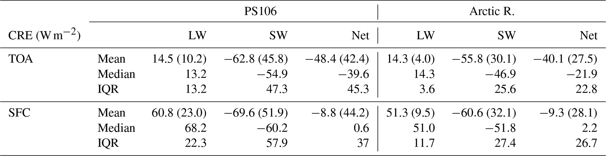
For the cruise track of the PS106 expedition, SW cooling by clouds dominates over LW warming, leading to a net cooling of −8.8 W m−2 at the SFC (see Table 3). For a similar time period, the net CRE at the SFC was also investigated by two other studies, both reporting stronger cooling. For Ny-Ålesund, NO, Ebell et al. (2020) find values within a range of about −20 to −40 W m−2 (see Fig. 6c in Ebell et al., 2020). Considering SW CRE, the study of Stapf et al. (2020) focused on the ACLOUD airborne campaign, calculated a mean SW CRE at the SFC of −32 W m−2. However, by considering a proposed cloud-free retrieval of α, taking spectral effects into account, this value increases to −62 W m−2, which is similar to our result of −68.8 W m−2 (see Table 3). It is worth noting that Ebell et al. (2020) explicitly take the effects of white-sky and black-sky albedo, and values obtained by CERES SYN1deg represent a cloud-free albedo (Chen et al., 2006) into account. Due to the strong sensitivity of SW CRE to α, a critical assessment of the accuracy of α used by CERES SYN1deg, including spectral and directionality effects, e.g. with in situ observations, is recommended.
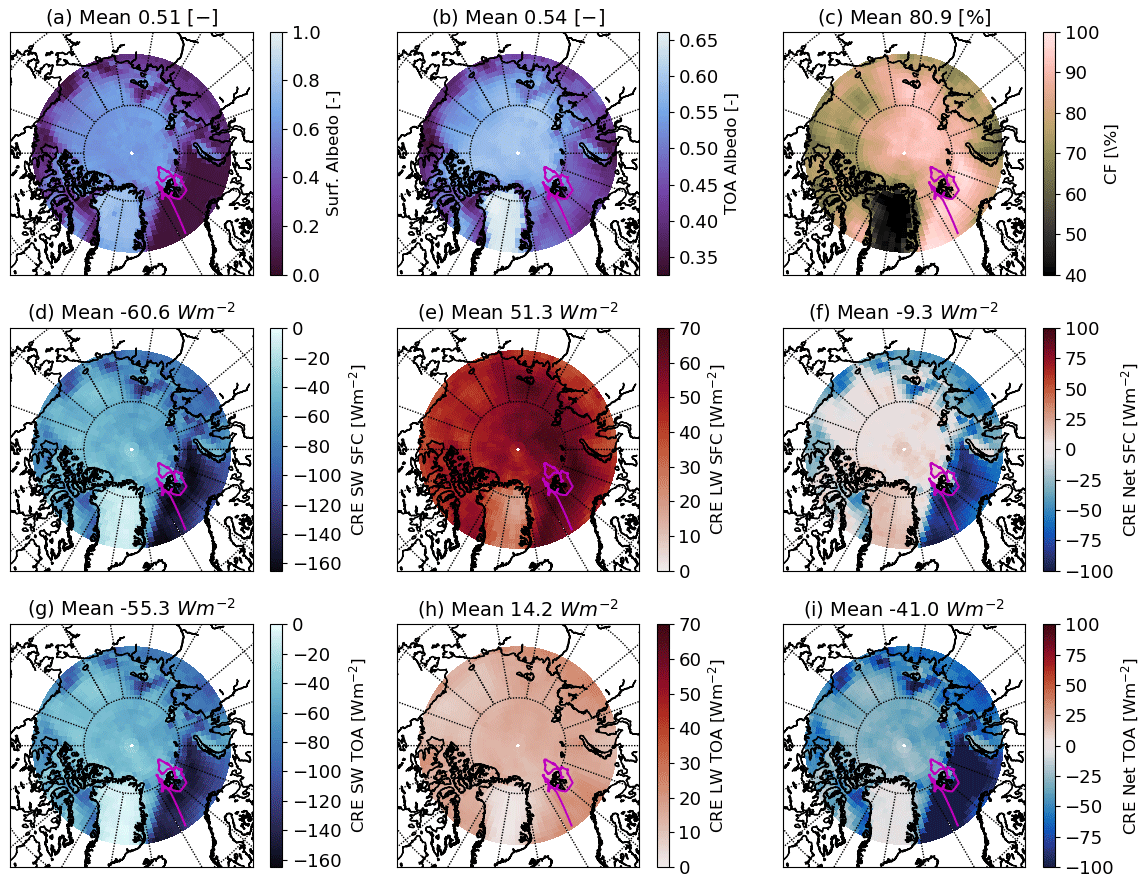
Figure 17Maps of several time-averaged CERES SYN1deg data sets for the Arctic (70 to 90∘ N) and the time period of the PS106 expedition. Panel (a) shows the mean surface albedo (α), (b) the top of the atmosphere (TOA) albedo, and (c) the mean cloud fraction (CF). Panels (d), (e), and (f) show the CRE for the SW, LW, and net spectral regions, respectively, at the surface (SFC), while panels (g), (h), and (i) present the same at the TOA. An orthographic projection is used, and the PS106 cruise track is indicated in magenta.
A similar analysis has been applied to the entire Arctic to embed the results obtained for PS106 in a wider context. Panels (f) and (i) of Fig. 17 show the mean CRE at the SFC and TOA for the entire time period of PS106, respectively. Additionally, the mean α, the TOA albedo, and the CF are shown in panels (a), (b), and (c), respectively.
For the considered time period and the Arctic region, a larger CF is found over open ocean than over land. This might be attributed to an increase of lower-tropospheric stability over land, which inhibits the mixing between the free troposphere and cloud layer, thus reducing CF (Morrison et al., 2012). The latter effect is most evident over the Barents Sea, central Arctic, Baffin Bay, and Siberian Sea (Fig. 17c). Over sea ice, CF is also large, with a particularly high occurrence of low and mid-low level clouds (not shown).
Based on CERES SYN1deg, low-level clouds are frequently found over the entire Arctic Ocean, with enhanced occurrence frequencies over the Barents Sea, Kara Sea, Laptev Sea, and the central Arctic. Mid-level clouds are mainly present over Greenland, East Arctic-Russia, Ellesmere Island and the central Arctic Ocean. High-level clouds occur more frequently over land, specifically over the Arctic-Russia, near Iqaluit in Canada, north of Sweden, Finland, and Norway (not shown). The spatial distribution of CF as visible in Fig. 17c, is consistent with the results of Palm et al. (2010) who report about an anticorrelation between sea-ice extent and CF based on satellite-based lidar measurements from the CALIOP mission for a 5-year period.
Differences in the spatial distribution of CF yield differences in CRE values both at the SFC and TOA. As indicated by Fig. 17f, the CRESFC is highly dependent on α, suggesting a warming effect of clouds by up to 20.5 W m−2 over highly reflective regions covered by snow/sea ice (Fig. 17a). At the TOA, the CRE shows a similar dependence on α, but with a stronger cooling effect. The mean CRE for the considered period is −9.3 W m−2 at the SFC, while it is −40.1 W m−2 at the TOA (see Table 3). The TOA albedo depends on CF and α. Low values are only expected for CS conditions over ocean, while high values correspond to either snow-covered or opaque clouds. This effect is, in particular, visible for the Barents Sea area, which corresponds to open ocean with a low α (Fig. 17a). Thus, the relatively high values found in Fig. 17b are caused by the frequent occurrence of clouds, as indicated in Fig. 17c. This region is of particular interest because mean values of CRE at the TOA and SFC are larger than for the rest of the Arctic.
Intrieri et al. (2002)Sedlar et al. (2011)de Boer et al. (2011)Miller et al. (2015)Wang et al. (2019)Ebell et al. (2020)Stapf et al. (2020)Stapf et al. (2021)Dong et al. (2010)Kay and L'Ecuyer (2013)Table 4Summary of literature comparison of the cloud radiative effect (CRE) at the surface (CRESFC) from different studies. Values in parentheses indicate the mean for the entire study.
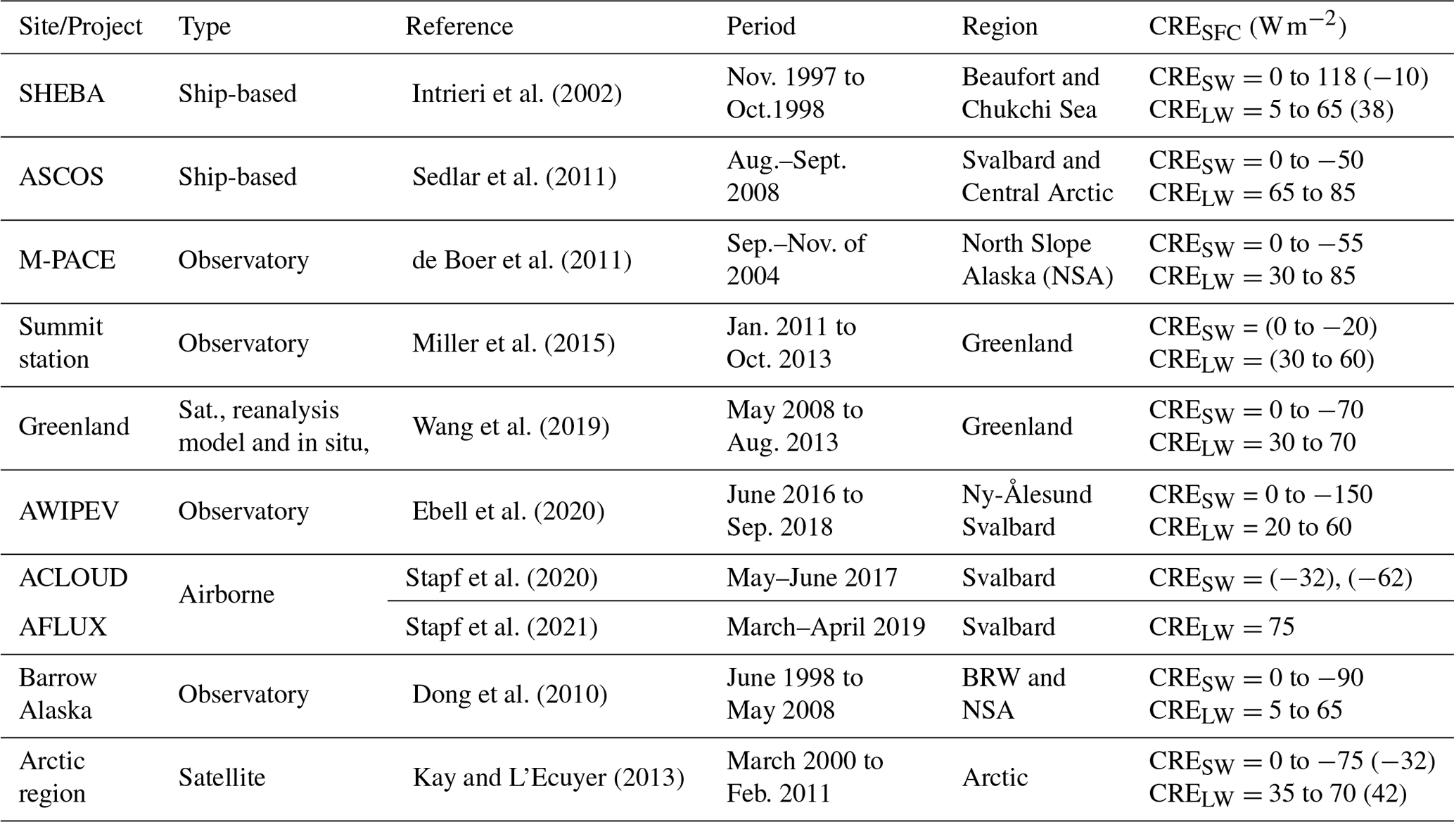
Previous studies have also investigated the CRESFC in the Arctic; see Table 4 for a list. The SHEBA expedition carried out observations in the Beaufort and Chukchi seas, and its observations were used to estimate the CRESFC for an entire annual cycle. Based on SHEBA, Intrieri et al. (2002) concluded that clouds warm the surface for most of the year. During early July, however, a cooling effect of the surface by about −4 W m−2 was found. Based on the Arctic Summer Cloud Ocean Study (ASCOS) shipborne campaign, CRESFC was also calculated, finding a warming effect, with values ranging from 5 to about 75 W m−2 (see Fig. 8 in Sedlar et al., 2011). Long-term observations can be used to resolve details of the annual cycle. Based on 10 year observations at NSA and the National Oceanic and Atmospheric Administration's (NOAA) Barrow Observatory (BRW) sites, the analysis of Dong et al. (2010) found a CRESFC ranging from −15 to −35 W m−2 for the time period from end of May to mid-July (see Fig. 3 in Dong et al., 2010). In contrast, the mixed-phase Arctic Clouds Experiment (M-PACE) conducted at the NSA site found a CRESFC ranging from 40 to 80 W m−2 for the months from September–December (de Boer et al., 2011), which is significantly larger than values reported by Dong et al. (2010).
In contrast to the remainder of the Arctic, Greenland is covered by ice and snow during the entire year. Clouds have a warming effect during the entire annual cycle, with the highest values of CRE found from July–August (see Fig. 5 in Miller et al., 2015). Miller et al. (2015) report values within a range of about 25 to 45 W m−2, which is larger than the mean values reported here, reaching a maximum of 20.5 W m−2 over Greenland (see Fig. 17).
Kay and L'Ecuyer (2013) derived the CRE based on a combination of active and passive satellite-based remote-sensing observations over the Arctic Ocean, and report a mean CRESFC of about −30 to −40 W m−2 at the surface for the period from the end of May to mid-July. These values are evidently larger than the mean value of −9.3 W m−2 found in the present study. However, the results of Kay and L'Ecuyer (2013) focus mostly on the Arctic Ocean and exclude Greenland.
The comparison and discussion of our results with previous studies provide valuable context on the CRE across the Arctic for different seasons and locations. Nevertheless, it is worth noting that such a comparison cannot fully account for all factors affecting the results, including the consideration of particular sites, regions, cloud conditions, seasons, data sets, methods to obtain α, and different temporal averaging.
This study investigated the characteristics of Arctic clouds, and their effect on radiative fluxes and the radiation budget during Polarstern's PS106 cruise held in the early summer of 2017. An intercomparison of cloud properties, derived from the shipborne cloud remote-sensing observations using the CERES SYN1deg ed. 4.1 satellite products, was first conducted, followed by an intercomparison of radiative fluxes from shipborne observations, radiative transfer simulations, and CERES. For this purpose, a radiative transfer setup for the simulation of SW and LW fluxes, denoted as T-CARS, was implemented using atmospheric profiles from the ERA5 reanalysis, Cloudnet cloud products, and other ancillary data as input. This setup has also been used to quantify the sensitivity of CS radiative fluxes to various input parameters.
Considering the different perspectives and sensitivities of the satellite and shipborne remote-sensing observations, the horizontally resolved field of view of CERES SYN1deg, and the vertically resolved view of the active remote- sensing instruments aboard Polarstern are found to offer complementary information on Arctic clouds.
A list of the main conclusions of this paper is given here:
-
Based on the CERES SYN1deg (Cloudnet) products, clouds occurred for about 86.7 % (76.1 %) of the time during PS106. Differences between the CERES SYN1deg and Cloudnet are mainly due to the different spatial resolution, data gaps, and moments of misidentifying clouds by Cloudnet. In the case studies, situations were identified where CERES SYN1deg underestimates high-level clouds, likely due to previously reported limitations of CERES SYN1deg products in polar regions (Trepte et al., 2019; Sun-Mack et al., 2018).
-
A case study comparing the CERES SYN1deg products (T-CARS simulations) with ship-based observations of downward fluxes in CS conditions yields satisfactory agreement, with flux mean differences of −13 W m−2 (−13.6 W m−2) for LWD, and −2.1 W m−2 (−7.9 W m−2) for SWD. This finding holds, despite the harsh environmental conditions and shipborne operation, which likely increase the instrumental uncertainties (estimated to be ±20 W m−2 for pyranometer/SWD and ±13 W m−2 for pyrgeometers/LWD). While the T-CARS simulations currently neglect aerosol effects, the CERES SYN1deg products suggest that on average, aerosols increase the LWD flux by 0.5 W m−2, and decrease SWD by 10.8 W m−2 (Fig. B1), confirming that aerosol effects are minor for LW and only relevant for SW.
-
For AS conditions, CERES SYN1deg surface radiative fluxes and observations agree well during PS106, with a mean difference of 6.0 and 23.1 W m−2 for SWD and LWD, respectively. The comparison yields a R2 of 0.69 (0.77) and RMSE of 12.2 W m−2 (46.5 W m−2) for LWD (SWD). These results are consistent with the findings by Dong et al. (2016), and Riihelä et al. (2017), who also performed comparisons between in situ radiative fluxes and CERES SYN1deg products at the ARM NSA site, as well as the Tara ice camp, and on the Greenland Ice Sheet, respectively. Instrumental limitations arise from the ship-based operation of instruments and the harsh environmental conditions, which cause a reduced accuracy of the observed radiative fluxes, and limits their accuracy for radiative closure studies.
-
Based on the CERES SYN1deg products, the mean radiation budget has been estimated along the cruise track and for the entire Arctic for the period of PS106. A dominating contribution of the SW radiation to the SRB is found, leading to a net SFC flux of 88.8, and 94.4 W m−2 for PS106 and the entire Arctic, respectively. Moreover, the effect of clouds on the radiation budget has been investigated. The mean net CRE during PS106 along the cruise track is −8.8 W m−2 at the SFC and −48.4 W m−2 at the TOA, implying an atmospheric cooling of 39.6 W m−2 (Table 3). For the entire Arctic, the net CRE is similar to PS106, with values of −9.3, and −40.1 W m−2, at the SFC and TOA, respectively (Fig. 17). The similarity of the local and regional CRE suggests that the PS106 cloud observations along the cruise track are representative of the cloud conditions found over the Arctic during this time of the year. Our results are also consistent with the summer results obtained from Ebell et al. (2020), who calculated the CRE during 2017 at Ny-Ålesund – NO (see their Fig. 6).
In the future, we plan to carry out a similar analysis based on observations from the MOSAiC expedition. This will extend the temporal coverage of observations to a full annual cycle in the central Arctic, and thus increase the climatological relevance of findings.
The radiative closure assessment using shipborne remote-sensing observations as input for the T-CARS simulations has been limited to specific cases in the present study. An extension to the full period of the cruise would allow a more in-depth investigation of the accuracy of the Cloudnet cloud products for specific cloud conditions. Particular attention should be given to the accuracy of the Cloudnet retrievals for relatively low values of QL and QI. For MOSAiC, cloud products based on the Shupe–Turner retrievals (Shupe et al., 2015) and distributed by ARM will also be available, allowing for a comparison of the Cloudnet and ARM products with respect to their ability to accurately represent the optical properties of Arctic clouds. Particular attention will be given to periods when the LW radiative properties are sensitive to small changes in QL (e.g. <50 g m−2; Turner, 2007; Tjernström et al., 2015; Achtert et al., 2020), which have been found to be poorly captured in our study. Moreover, given the importance of α and Ts to the interpretation of the radiation budget, it is planned to evaluate the local values observed during MOSAiC to the values used in this study.
Satellite observations and products are necessary to extend the analysis of CREs to a wider regional and decadal perspective. This would allow the investigation of long-term changes of CRE and the radiation budget. To contribute to the latter, we acknowledge the particular importance of the LW radiation budget across the entire annual cycle in the Arctic region (Sedlar and Tjernström, 2017). Therefore, we will expand our analysis by implementing radiative kernel techniques to diagnose climate feedback based on ground-based and satellite remote-sensing observations (Soden et al., 2008; Tan and Storelvmo, 2019).
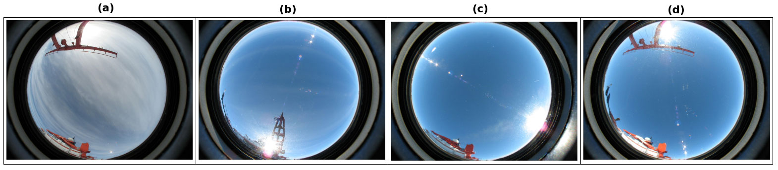
Figure A1Sky-camera photographs for 2 July 2017 04:00:08 Z (a), 2 July 2017 12:13:33 Z (b), 3 July 2017 04:14:09 Z (c), and 3 July 2017 12:04:08 Z (d). All times in UTC.
Table A1Results of the sensitivity analysis, varying several atmospheric parameters. The table indicates the mean upward (U) and downward (D) SW and LW flux differences at the surface of clear-sky (CS) perturbed simulations minus idealized atmosphere simulation. Values in W m−2. Values highlighted in bold are used as uncertainties.
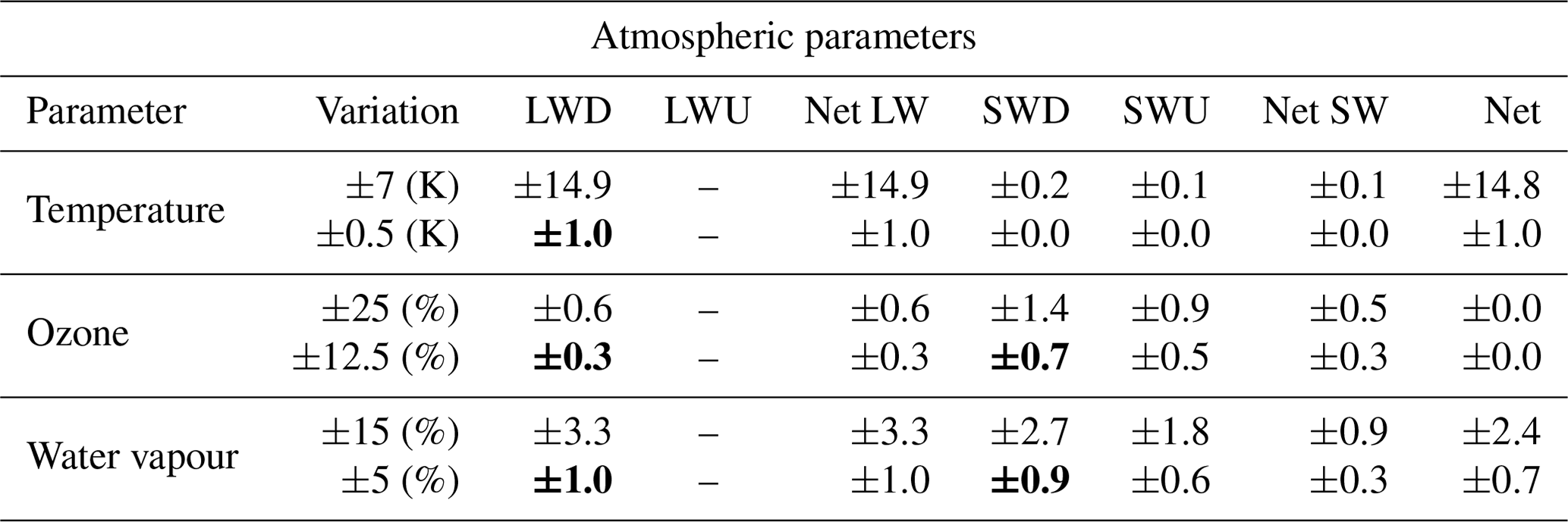
Table A2Variation of several surface parameters. The table indicates the mean upward (U) and downward (D) SW and LW flux differences at the surface of clear-sky (CS) perturbed simulations minus idealized atmosphere simulation. Values in W m−2. Values highlighted in bold are used as uncertainties.
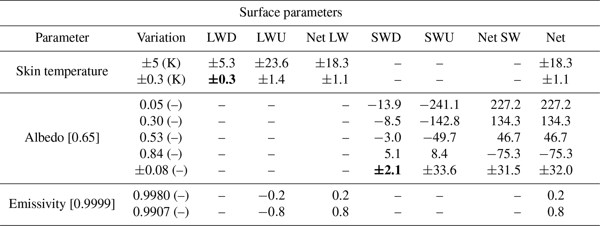
Table A3Variation of several atmospheric parameters. The table indicates the mean upward SW (SWU), LW (LWU), and net flux differences at the top of the atmosphere (TOA) of clear-sky (CS) perturbed simulations minus the created idealized atmosphere. Values in W m−2. Values highlighted in bold are used as uncertainties.
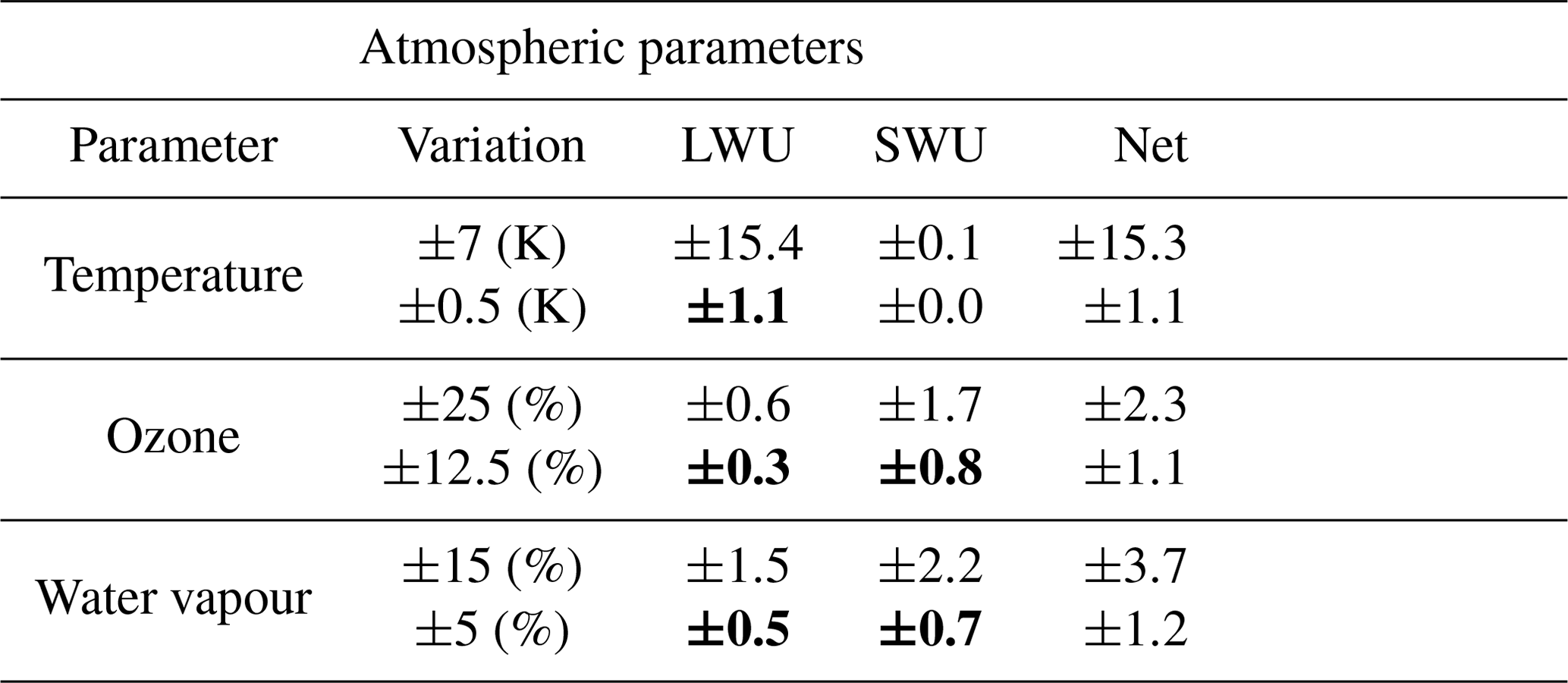
Table A4The table indicates the mean upward SW (SWU), LW (LWU), and net flux differences at the top of the atmosphere (TOA) of clear-sky (CS) perturbed simulations minus idealized atmosphere simulation. Values in W m−2. Values highlighted in bold are used as uncertainties.
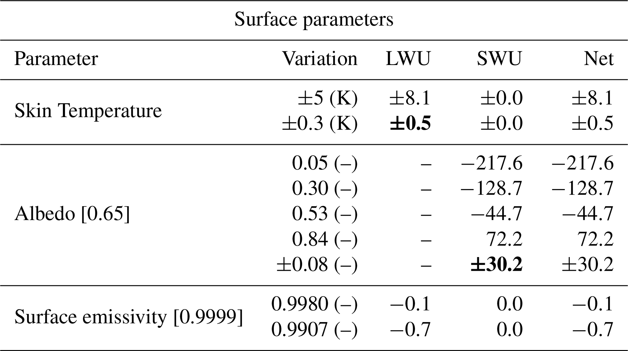
Table B1Radiation budget for PS106 for all-sky (AS) and clear-sky (CS) conditions based on the CERES SYN1deg data set. Values represent mean and standard deviation (in parentheses) from 28 May to 20 June, 22 June to 16 July 2017.
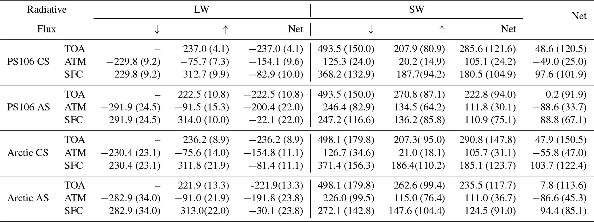
Table B2Radiation budget for PS106 for pristine (P) and cloudy without aerosols (NA) conditions based on the CERES SYN1deg data set from 28 May to 20 June, and 22 June to 16 July 2017.
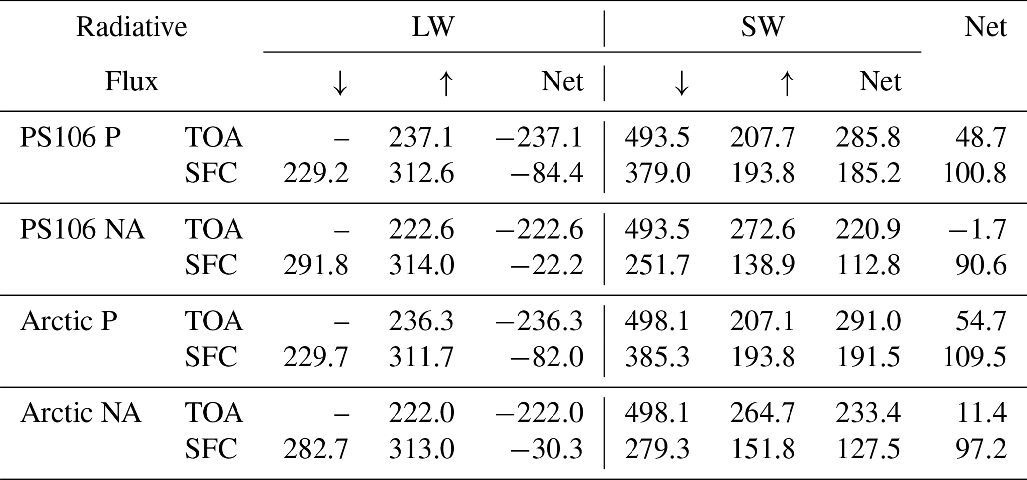
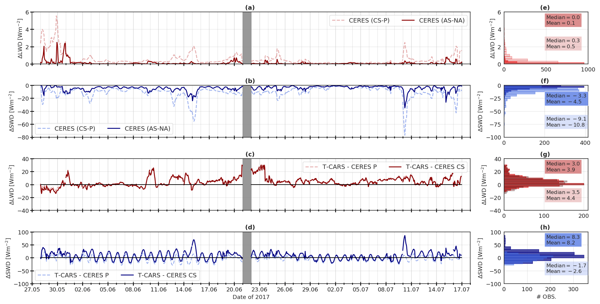
Figure B1Time series of the difference of downward surface radiative fluxes between CERES SYN1deg and T-CARS for pristine (P), clear-sky (CS), all-sky (AS), and cloudy without aerosols (NA) conditions. Panel (a) shows the difference of the downward LW (LWD) CERES SYN1deg (CS-P) and CERES SYN1deg (AS-NA). Panel (b) shows the same as (a), but the downward SW (SWD) flux. Panel (c) shows the LWD differences between T-CARS and CERES SYN1deg P, and T-CARS minus CERES SYN1deg CS. The histograms of each left-hand side panel are shown on the right. The LWD and SWD fluxes are shown in red and blue, respectively.
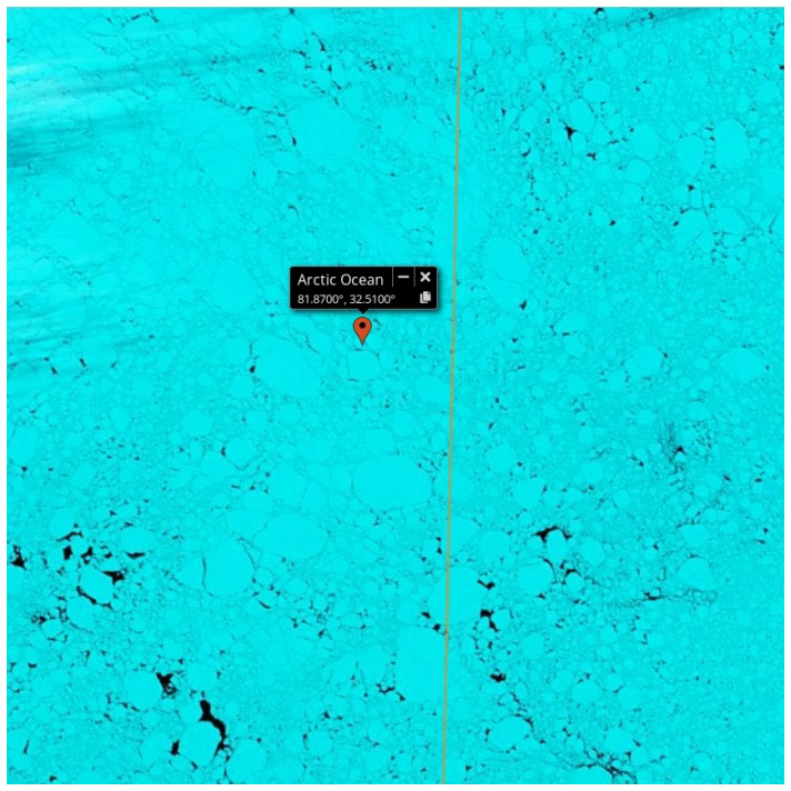
Figure C1Moderate Resolution Imaging Spectroradiometer (MODIS) screenshot for 3 July 2017. The red symbol indicates Polarstern's location. The orange line indicates the MODIS track. Image obtained from EOSDIS Worldview 2021 Version 3.15.

Figure C2Same as Fig. C1, but for 2 July 2017. Image obtained from EOSDIS Worldview 2021 Version 3.15.
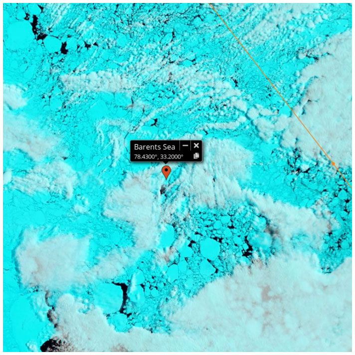
Figure C3Same as Fig. C1, but for 26 June 2017. Image obtained from EOSDIS Worldview 2021 Version 3.15.
The analysed Cloudnet data are available at Griesche et al. (2020a) (https://doi.org/10.1594/PANGAEA.919463), Griesche et al. (2020b) (https://doi.org/10.1594/PANGAEA.919452), Griesche et al. (2020c) (https://doi.org/10.1594/PANGAEA.919383), Griesche et al. (2020d) (https://doi.org/10.1594/PANGAEA.919386), and Griesche et al. (2020e) (https://doi.org/10.1594/PANGAEA.919399). The analysis of low-level stratus (LLS) clouds introduced in Griesche et al. (2020) is based on the data set available at Griesche et al. (2020f) (https://doi.org/10.1594/PANGAEA.920246).
The data used for surface parameters based on single-layer hourly ERA5 data are available at Hersbach et al. (2018b) (https://doi.org/10.24381/cds.adbb2d47) and for pressure levels are available at Hersbach et al. (2018a) (https://doi.org/10.24381/cds.bd0915c6).
The CERES SYN1deg products were obtained from the NASA Langley Research Center Atmospheric Science Data Center, which is available at NASA/LARC/SD/ASDC (2017) (https://doi.org/10.5067/TERRA+AQUA/CERES/SYN1DEG-1HOUR_L3.004A).
The T-CARS simulations are available at Barrientos Velasco et al. (2021) (https://doi.org/10.5281/zenodo.5725382).
CBV, HD and AH conceptualized the manuscript. PS and HJG were responsible for the data curation of the observations. CBV performed the formal analysis, methodology, visualization and writing of the original draft preparation. AM was responsible for the funding acquisition and the project administration. All authors contributed to the subsequent improvement of the analysis and editing of the manuscript.
The contact author has declared that neither they nor their co-authors have any competing interests.
Publisher's note: Copernicus Publications remains neutral with regard to jurisdictional claims in published maps and institutional affiliations.
This article is part of the special issue “Arctic mixed-phase clouds as studied during the ACLOUD/PASCAL campaigns in the framework of (AC)³ (ACP/AMT/ESSD inter-journal SI)”. It is not associated with a conference.
We gratefully acknowledge funding by the Deutsche Forschungsgemeinschaft (DFG, German Research Foundation) – Project Number 268020496 – TRR 172, within the Transregional Collaborative Research Center “ArctiC Amplification: Climate Relevant Atmospheric and SurfaCe Processes, and Feedback Mechanisms (AC)3” during phase I, and by the Bundesministerium für Bildung und Forschung for the project “Combining MOSAiC and Satellite Observations for Radiative Closure and Climate Implications” (MOSARiCs) – Project Number 03F0890A. We thank Captain Thomas Wunderlich and the entire crew of Polarstern for their logistic support. We also thank our colleagues at AWI, DWD, Leipziger Institut für Meteorologie and TROPOS for their logistic support and scientific cooperation. We thank the anonymous reviewers, for their suggestions and comments, which significantly improved the final version of this manuscript. We would like to acknowledge the Copernicus Climate Change Service (C3S) for making their ERA5 products easily accessible. Similarly, we deeply acknowledge the NASA Langley Research Center Atmospheric Science Data Center for making available their products for the analysis of this study.
This research has been supported by the Deutsche Forschungsgemeinschaft (grant no. 268020496) and the Bundesministerium für Bildung und Forschung for the project “Combining MOSAiC and Satellite Observations for Radiative Closure and Climate Implications” (MOSARiCs) (project no. 03F0890A).
This paper was edited by Radovan Krejci and reviewed by two anonymous referees.
Achtert, P., O'Connor, E. J., Brooks, I. M., Sotiropoulou, G., Shupe, M. D., Pospichal, B., Brooks, B. J., and Tjernström, M.: Properties of Arctic liquid and mixed-phase clouds from shipborne Cloudnet observations during ACSE 2014, Atmos. Chem. Phys., 20, 14983–15002, https://doi.org/10.5194/acp-20-14983-2020, 2020. a
Anderson, G., Clough, S., Kneizys, F., Chetwynd, J., and Shettle, E.: AFGL Atmospheric Constituent Profiles (0.120km), p. 46, 1986. a, b, c
Anstey, J. A. and Shepherd, T. G.: High-latitude influence of the quasi-biennial oscillation, Q. J. Roy. Meteor. Soc., 140, 1–21, 2014. a
Bahramvash Shams, S., Walden, V. P., Petropavlovskikh, I., Tarasick, D., Kivi, R., Oltmans, S., Johnson, B., Cullis, P., Sterling, C. W., Thölix, L., and Errera, Q.: Variations in the vertical profile of ozone at four high-latitude Arctic sites from 2005 to 2017, Atmos. Chem. Phys., 19, 9733–9751, https://doi.org/10.5194/acp-19-9733-2019, 2019. a, b
Ballinger, T. J., Overland, J. E., Wang, M., Bhatt, U. S., Hanna, E., Hanssen-Bauer, I., Kim, S. J., Thoman, R. L., and Walsh, J. E.: Surface Air Temperature, United States. National Oceanic and Atmospheric Administration. Office of Oceanic and Atmospheric Research. Pacific Marine Environmental Laboratory (U.S.) Cooperative Institute for Climate, Ocean, and Ecosystem Studies International Arctic Research Center University of Alaska Fairbanks. Geophysical Institute University of Lincoln Norske meteorologiske institutt/Norwegian Meteorological Institute Han’guk Haeyang Yŏn’guwŏn. Pusŏl Kŭkchi Yŏn’guso/Korea Polar Research Institute, https://doi.org/10.25923/gcw8-2z06, 2020. a
Barker, H. W., Stephens, G. L., Partain, P. T., Bergman, J. W., Bonnel, B., Campana, K., Clothiaux, E. E., Clough, S., Cusack, S., Delamere, J., Edwards, J., Evans, K. F., Fouquart, Y., Freidenreich, S., Galin, V., Hou, Y., Kato, S., Li, J., Mlawer, E., Morcrette, J.-J., O'Hirok, W., Räisänen, P., Ramaswamy, V., Ritter, B., Rozanov, E., Schlesinger, M., Shibata, K., Sporyshev, P., Sun, Z., Wendisch, M., Wood, N., and Yang, F.: Assessing 1D Atmospheric Solar Radiative Transfer Models: Interpretation and Handling of Unresolved Clouds, J. Climate, 16, 2676–2699, https://doi.org/10.1175/1520-0442(2003)016<2676:ADASRT>2.0.CO;2, 2003. a
Barlakas, V., Deneke, H., and Macke, A.: The sub-adiabatic model as a concept for evaluating the representation and radiative effects of low-level clouds in a high-resolution atmospheric model, Atmos. Chem. Phys., 20, 303–322, https://doi.org/10.5194/acp-20-303-2020, 2020. a
Barrientos Velasco, C., Deneke, H., Griesche, H., Seifert, P., Engelmann, R., and Macke, A.: Spatiotemporal variability of solar radiation introduced by clouds over Arctic sea ice, Atmos. Meas. Tech., 13, 1757–1775, https://doi.org/10.5194/amt-13-1757-2020, 2020. a, b, c, d
Barrientos Velasco, C., Deneke, H., and Hünerbein, A.: Radiative transfer simulations for the Arctic research expedition PS106, Zenodo [data set], https://doi.org/10.5281/zenodo.5725382, 2021. a
Bright, R. M. and O'Halloran, T. L.: Developing a monthly radiative kernel for surface albedo change from satellite climatologies of Earth's shortwave radiation budget: CACK v1.0, Geosci. Model Dev., 12, 3975–3990, https://doi.org/10.5194/gmd-12-3975-2019, 2019. a
Bühl, J., Seifert, P., Myagkov, A., and Ansmann, A.: Measuring ice- and liquid-water properties in mixed-phase cloud layers at the Leipzig Cloudnet station, Atmos. Chem. Phys., 16, 10609–10620, https://doi.org/10.5194/acp-16-10609-2016, 2016. a
Chen, Y., Sun-Mack, S., Arduini, R., and Minnis, P.: Clear-sky and surface narrowband albedo variations derived from VIRS and MODIS data, 12th Conference on Cloud Physics, and 12th Conference on Atmospheric Radiation, 10–14 July 2006, Madison, WI, 2006. a
Christensen, M. W., Behrangi, A., L’ecuyer, T. S., Wood, N. B., Lebsock, M. D., and Stephens, G. L.: Arctic Observation and Reanalysis Integrated System: A New Data Product for Validation and Climate Study, B. Am. Meteorol. Soc., 97, 907–916, https://doi.org/10.1175/BAMS-D-14-00273.1, 2016. a
Clough, S., Shephard, M., Mlawer, E., Delamere, J., Iacono, M., Cady-Pereira, K., Boukabara, S., and Brown, P.: Atmospheric radiative transfer modeling: a summary of the AER codes, J. Quant. Spectrosc. Ra., 91, 233–244, https://doi.org/10.1016/j.jqsrt.2004.05.058, 2005. a
Collins, W. D., Rasch, P. J., Eaton, B. E., Khattatov, B. V., Lamarque, J.-F., and Zender, C. S.: Simulating aerosols using a chemical transport model with assimilation of satellite aerosol retrievals: Methodology for INDOEX, J. Geophys. Res.-Atmos., 106, 7313–7336, https://doi.org/10.1029/2000JD900507, 2001. a
Curry, J. A., Schramm, J. L., Rossow, W. B., and Randall, D.: Overview of Arctic Cloud and Radiation Characteristics, J. Climate, 9, 1731–1764, https://doi.org/10.1175/1520-0442(1996)009<1731:OOACAR>2.0.CO;2, 1996. a
de Boer, G., Collins, W. D., Menon, S., and Long, C. N.: Using surface remote sensors to derive radiative characteristics of Mixed-Phase Clouds: an example from M-PACE, Atmos. Chem. Phys., 11, 11937–11949, https://doi.org/10.5194/acp-11-11937-2011, 2011. a, b
Delamere, J. S., Clough, S. A., Payne, V. H., Mlawer, E. J., Turner, D. D., and Gamache, R. R.: A far-infrared radiative closure study in the Arctic: Application to water vapor, J. Geophys. Res.-Atmos., 115, https://doi.org/10.1029/2009JD012968, 2010. a
Delanoë, J., Protat, A., Bouniol, D., Heymsfield, A., Bansemer, A., and Brown, P.: The Characterization of Ice Cloud Properties from Doppler Radar Measurements, J. Appl. Meteorol. Clim., 46, 1682–1698, https://doi.org/10.1175/JAM2543.1, 2007. a
Deshler, T., Stübi, R., Schmidlin, F. J., Mercer, J. L., Smit, H. G. J., Johnson, B. J., Kivi, R., and Nardi, B.: Methods to homogenize electrochemical concentration cell (ECC) ozonesonde measurements across changes in sensing solution concentration or ozonesonde manufacturer, Atmos. Meas. Tech., 10, 2021–2043, https://doi.org/10.5194/amt-10-2021-2017, 2017. a
Devasthale, A., Sedlar, J., Kahn, B. H., Tjernström, M., Fetzer, E. J., Tian, B., Teixeira, J., and Pagano, T. S.: A Decade of Spaceborne Observations of the Arctic Atmosphere: Novel Insights from NASA’s AIRS Instrument, B. Am. Meteorol. Soc., 97, 2163–2176, https://doi.org/10.1175/BAMS-D-14-00202.1, 2016. a
Di Biagio, C., di Sarra, A., Eriksen, P., Ascanius, S. E., Muscari, G., and Holben, B.: Effect of surface albedo, water vapour, and atmospheric aerosols on the cloud-free shortwave radiative budget in the Arctic, Clim. Dynam., 39, 953–969, 2012. a, b
Dolinar, E. K., Dong, X., Xi, B., Jiang, J. H., and Loeb, N. G.: A clear-sky radiation closure study using a one-dimensional radiative transfer model and collocated satellite-surface-reanalysis data sets, J. Geophys. Res.-Atmos., 121, 13698–13714, https://doi.org/10.1002/2016JD025823, 2016. a
Dong, X., Xi, B., Crosby, K., Long, C. N., Stone, R. S., and Shupe, M. D.: A 10 year climatology of Arctic cloud fraction and radiative forcing at Barrow, Alaska, J. Geophys. Res.-Atmos., 115, https://doi.org/10.1029/2009JD013489, 2010. a, b, c, d
Dong, X., Xi, B., Qiu, S., Minnis, P., Sun-Mack, S., and Rose, F.: A radiation closure study of Arctic stratus cloud microphysical properties using the collocated satellite-surface data and Fu-Liou radiative transfer model, J. Geophys. Res.-Atmos., 121, 10175–10198, https://doi.org/10.1002/2016JD025255, 2016. a, b, c, d, e
Doyle, J. G., Lesins, G., Thackray, C. P., Perro, C., Nott, G. J., Duck, T. J., Damoah, R., and Drummond, J. R.: Water vapor intrusions into the High Arctic during winter, Geophys. Res. Lett., 38, https://doi.org/10.1029/2011GL047493, 2011. a
Eastwood, S., Lavergne, T., and Tonboe, R.: Algorithm theoretical basis document for the OSI SAF global reprocessed sea ice concentration product, EUMETSAT Network Satellite Application Facilities, 28, https://osisaf-hl.met.no/sites/osisaf-hl.met.no/files/baseline_document/osisaf_cdop2_ss2_atbd_sea-ice-conc-reproc_v1p1.pdf (last access: 15 July 2022), 2014. a
Ebell, K., Nomokonova, T., Maturilli, M., and Ritter, C.: Radiative Effect of Clouds at Ny-Ålesund, Svalbard, as Inferred from Ground-Based Remote Sensing Observations, J. Appl. Meteorol. Clim., 59, 3–22, https://doi.org/10.1175/JAMC-D-19-0080.1, 2020. a, b, c, d, e, f, g, h
Egerer, U., Ehrlich, A., Gottschalk, M., Griesche, H., Neggers, R. A. J., Siebert, H., and Wendisch, M.: Case study of a humidity layer above Arctic stratocumulus and potential turbulent coupling with the cloud top, Atmos. Chem. Phys., 21, 6347–6364, https://doi.org/10.5194/acp-21-6347-2021, 2021. a
Frisch, A. S., Feingold, G., Fairall, C. W., Uttal, T., and Snider, J. B.: On cloud radar and microwave radiometer measurements of stratus cloud liquid water profiles, J. Geophys. Res.-Atmos., 103, 23195–23197, https://doi.org/10.1029/98JD01827, 1998. a
Frisch, S., Shupe, M., Djalalova, I., Feingold, G., and Poellot, M.: The Retrieval of Stratus Cloud Droplet Effective Radius with Cloud Radars, J. Atmos. Ocean. Tech., 19, 835–842, https://doi.org/10.1175/1520-0426(2002)019<0835:TROSCD>2.0.CO;2, 2002. a, b
Fu, Q. and Liou, K. N.: On the Correlated k-Distribution Method for Radiative Transfer in Nonhomogeneous Atmospheres, J. Atmos. Sci., 49, 2139–2156, https://doi.org/10.1175/1520-0469(1992)049<2139:OTCDMF>2.0.CO;2, 1992. a
Griesche, H., Seifert, P., Engelmann, R., Radenz, M., and Bühl, J.: Cloudnet target classification during PS106, PANGAEA [data set], https://doi.org/10.1594/PANGAEA.919463, 2020a. a
Griesche, H., Seifert, P., Engelmann, R., Radenz, M., and Bühl, J.: Cloudnet IWC during PS106, PANGAEA [data set], https://doi.org/10.1594/PANGAEA.919452, 2020b. a
Griesche, H., Seifert, P., Engelmann, R., Radenz, M., and Bühl, J.: Cloudnet LWC during PS106, PANGAEA [data set], https://doi.org/10.1594/PANGAEA.919383, 2020c. a
Griesche, H., Seifert, P., Engelmann, R., Radenz, M., and Bühl, J.: Cloudnet ice particles effective radius during PS106, PANGAEA [data set], https://doi.org/10.1594/PANGAEA.919386, 2020d. a
Griesche, H., Seifert, P., Engelmann, R., Radenz, M., and Bühl, J.: Cloudnet liquid droplet effective radius during PS106, PANGAEA [data set], https://doi.org/10.1594/PANGAEA.919399, 2020e. a
Griesche, H., Seifert, P., Engelmann, R., Radenz, M., and Bühl, J.: OCEANET-ATMOSPHERE low level stratus clouds during PS106, PANGAEA [data set], https://doi.org/10.1594/PANGAEA.920246, 2020f. a
Griesche, H. J., Seifert, P., Ansmann, A., Baars, H., Barrientos Velasco, C., Bühl, J., Engelmann, R., Radenz, M., Zhenping, Y., and Macke, A.: Application of the shipborne remote sensing supersite OCEANET for profiling of Arctic aerosols and clouds during Polarstern cruise PS106, Atmos. Meas. Tech., 13, 5335–5358, https://doi.org/10.5194/amt-13-5335-2020, 2020. a, b, c, d, e, f, g, h, i, j, k, l, m, n, o, p, q, r
Gröbner, J. and Wacker, S.: Pyrgeometer Calibration Procedure at the PMOD/WRC-IRS, World Meteorological Organization, https://library.wmo.int/doc_num.php?explnum_id=7365 (last access: 13 July 2022), 2015. a
Gröbner, J., Reda, I., Wacker, S., Nyeki, S., Behrens, K., and Gorman, J.: A new absolute reference for atmospheric longwave irradiance measurements with traceability to SI units, J. Geophys. Res.-Atmos., 119, 7083–7090, https://doi.org/10.1002/2014JD021630, 2014. a
Gupta, S. K., Kratz, D. P., Stackhouse, Paul W., J., Wilber, A. C., Zhang, T., and Sothcott, V. E.: Improvement of Surface Longwave Flux Algorithms Used in CERES Processing, J. Appl. Meteorol. Clim., 49, 1579–1589, https://doi.org/10.1175/2010JAMC2463.1, 2010. a
Hanschmann, T., Deneke, H., Roebeling, R., and Macke, A.: Evaluation of the shortwave cloud radiative effect over the ocean by use of ship and satellite observations, Atmos. Chem. Phys., 12, 12243–12253, https://doi.org/10.5194/acp-12-12243-2012, 2012. a, b
Hartmann, D. L. and Ceppi, P.: Trends in the CERES Dataset, 2000–13: The Effects of Sea Ice and Jet Shifts and Comparison to Climate Models, J. Climate, 27, 2444–2456, https://doi.org/10.1175/JCLI-D-13-00411.1, 2014. a
Hersbach, H., Bell, B., Berrisford, P., Biavati, G., Horányi, A., Muñoz Sabater, J., Nicolas, J., Peubey, C., Radu, R., Rozum, I., Schepers, D., Simmons, A., Soci, C., Dee, D., and Thépaut, J.-N.: ERA5 hourly data on pressure levels from 1979 to present, Copernicus Climate Change Service (C3S) Climate Data Store (CDS) [data set], https://doi.org/10.24381/cds.bd0915c6, 2018a. a
Hersbach, H., Bell, B., Berrisford, P., Biavati, G., Horányi, A., Muñoz Sabater, J., Nicolas, J., Peubey, C., Radu, R., Rozum, I., Schepers, D., Simmons, A., Soci, C., Dee, D., and Thépaut, J.-N.: ERA5 hourly data on single levels from 1979 to present, Copernicus Climate Change Service (C3S) Climate Data Store (CDS) [data set], https://doi.org/10.24381/cds.adbb2d47, 2018b. a
Hersbach, H., Bell, B., Berrisford, P., Hirahara, S., Horányi, A., Muñoz-Sabater, J., Nicolas, J., Peubey, C., Radu, R., Schepers, D., Simmons, A., Soci, C., Abdalla, S., Abellan, X., Balsamo, G., Bechtold, P., Biavati, G., Bidlot, J., Bonavita, M., De Chiara, G., Dahlgren, P., Dee, D., Diamantakis, M., Dragani, R., Flemming, J., Forbes, R., Fuentes, M., Geer, A., Haimberger, L., Healy, S., Hogan, R. J., Hólm, E., Janisková, M., Keeley, S., Laloyaux, P., Lopez, P., Lupu, C., Radnoti, G., de Rosnay, P., Rozum, I., Vamborg, F., Villaume, S., and Thépaut, J.-N.: The ERA5 global reanalysis, Q. J. Roy. Meteor. Soc., 146, 1999–2049, https://doi.org/10.1002/qj.3803, 2020. a
Hirahara, S., Balmaseda, M. A., de Boisseson, E., and Hersbach, H.: 26 sea surface temperature and sea ice concentration for ERA5, Eur. Centre Medium Range Weather Forecasts, Berkshire, UK, ERA Rep. Ser, 26, https://www.ecmwf.int/sites/default/files/elibrary/2016/16555-sea-surface-temperature-and-sea-ice-concentration-era5.pdf (last access: 15 July 2022), 2016. a
Hogan, R. and Connor, E.: Facilitating cloud radar and lidar algorithms: the Cloudnet Instrument Synergy/Target Categorization product, http://www.met.rdg.ac.uk/~swrhgnrj/publications/categorization.pdf (last access: 13 July 2022), 2004. a
Hogan, R. J., Mittermaier, M. P., and Illingworth, A. J.: The Retrieval of Ice Water Content from Radar Reflectivity Factor and Temperature and Its Use in Evaluating a Mesoscale Model, J. Appl. Meteorol. Clim., 45, 301–317, https://doi.org/10.1175/JAM2340.1, 2006. a, b
Hogan, R. J., O'Connor, E. J., and Illingworth, A. J.: Verification of cloud-fraction forecasts, Q. J. Roy. Meteor. Soc., 135, 1494–1511, https://doi.org/10.1002/qj.481, 2009. a
Hori, M., Aoki, T., Tanikawa, T., Motoyoshi, H., Hachikubo, A., Sugiura, K., Yasunari, T. J., Eide, H., Storvold, R., Nakajima, Y., and Takahashi, F.: In-situ measured spectral directional emissivity of snow and ice in the 8–14 µm atmospheric window, Remote Sens. Environ., 100, 486–502, https://doi.org/10.1016/j.rse.2005.11.001, 2006. a
Hu, Y. X. and Stamnes, K.: An Accurate Parameterization of the Radiative Properties of Water Clouds Suitable for Use in Climate Models, J. Climate, 6, 728–742, https://doi.org/10.1175/1520-0442(1993)006<0728:AAPOTR>2.0.CO;2, 1993. a
Huang, Y., Dong, X., Xi, B., Dolinar, E. K., Stanfield, R. E., and Qiu, S.: Quantifying the Uncertainties of Reanalyzed Arctic Cloud and Radiation Properties Using Satellite Surface Observations, J. Climate, 30, 8007–8029, https://doi.org/10.1175/JCLI-D-16-0722.1, 2017. a, b, c
Illingworth, A. J., Hogan, R. J., O'Connor, E., Bouniol, D., Brooks, M. E., Delanoë, J., Donovan, D. P., Eastment, J. D., Gaussiat, N., Goddard, J. W. F., Haeffelin, M., Baltink, H. K., Krasnov, O. A., Pelon, J., Piriou, J.-M., Protat, A., Russchenberg, H. W. J., Seifert, A., Tompkins, A. M., van Zadelhoff, G.-J., Vinit, F., Willén, U., Wilson, D. R., and Wrench, C. L.: Cloudnet, B. Am. Meteorol. Soc., 88, 883–898, https://doi.org/10.1175/BAMS-88-6-883, 2007. a, b, c, d, e, f
Intrieri, J. M., Fairall, C. W., Shupe, M. D., Persson, P. O. G., Andreas, E. L., Guest, P. S., and Moritz, R. E.: An annual cycle of Arctic surface cloud forcing at SHEBA, J. Geophys. Res.-Oceans, 107, SHE 13-1–SHE 13-14, https://doi.org/10.1029/2000JC000439, 2002. a, b
Johannessen, O. M., Bengtsson, L., Miles, M. W., Kuzmina, S. I., Semenov, V. A., Alekseev, G. V., Nagurnyi, A. P., Zakharov, V. F., Bobylev, L. P., Pettersson, L. H., Hasselmann, K., and Cattle, H. P.: Arctic climate change: observed and modelled temperature and sea-ice variability, Tellus A, 56, 328–341, https://doi.org/10.1111/j.1600-0870.2004.00060.x, 2004. a
Kalesse, H., Vogl, T., Paduraru, C., and Luke, E.: Development and validation of a supervised machine learning radar Doppler spectra peak-finding algorithm, Atmos. Meas. Tech., 12, 4591–4617, https://doi.org/10.5194/amt-12-4591-2019, 2019. a
Kalisch, J. and Macke, A.: Radiative budget and cloud radiative effect over the Atlantic from ship-based observations, Atmos. Meas. Tech., 5, 2391–2401, https://doi.org/10.5194/amt-5-2391-2012, 2012. a, b
Kanitz, T., Ansmann, A., Engelmann, R., and Althausen, D.: North-south cross sections of the vertical aerosol distribution over the Atlantic Ocean from multiwavelength Raman/polarization lidar during Polarstern cruises, J. Geophys. Res.-Atmos., 118, 2643–2655, https://doi.org/10.1002/jgrd.50273, 2013. a, b
Karlsson, K.-G., Anttila, K., Trentmann, J., Stengel, M., Fokke Meirink, J., Devasthale, A., Hanschmann, T., Kothe, S., Jääskeläinen, E., Sedlar, J., Benas, N., van Zadelhoff, G.-J., Schlundt, C., Stein, D., Finkensieper, S., Håkansson, N., and Hollmann, R.: CLARA-A2: the second edition of the CM SAF cloud and radiation data record from 34 years of global AVHRR data, Atmos. Chem. Phys., 17, 5809–5828, https://doi.org/10.5194/acp-17-5809-2017, 2017. a
Kato, S., Rose, F. G., Rutan, D. A., Thorsen, T. J., Loeb, N. G., Doelling, D. R., Huang, X., Smith, W. L., Su, W., and Ham, S.-H.: Surface Irradiances of Edition 4.0 Clouds and the Earth’s Radiant Energy System (CERES) Energy Balanced and Filled (EBAF) Data Product, J. Climate, 31, 4501–4527, https://doi.org/10.1175/JCLI-D-17-0523.1, 2018. a
Kay, J. E. and L'Ecuyer, T.: Observational constraints on Arctic Ocean clouds and radiative fluxes during the early 21st century, J. Geophys. Res.-Atmos., 118, 7219–7236, https://doi.org/10.1002/jgrd.50489, 2013. a, b, c
Kay, J. E., L'Ecuyer, T., Chepfer, H., Loeb, N., Morrison, A., and Cesana, G.: Recent Advances in Arctic Cloud and Climate Research, Current Climate Change Reports, 2, 159–169, https://doi.org/10.1007/s40641-016-0051-9, 2016. a, b
Key, J.: Streamer user's guide, Tech. Rep., Boston University, 96–01, 85, https://geocryos.ssec.wisc.edu/streamer/userman.pdf (last access: 15 July 2022), 1996. a
Knudsen, E. M., Heinold, B., Dahlke, S., Bozem, H., Crewell, S., Gorodetskaya, I. V., Heygster, G., Kunkel, D., Maturilli, M., Mech, M., Viceto, C., Rinke, A., Schmithüsen, H., Ehrlich, A., Macke, A., Lüpkes, C., and Wendisch, M.: Meteorological conditions during the ACLOUD/PASCAL field campaign near Svalbard in early summer 2017, Atmos. Chem. Phys., 18, 17995–18022, https://doi.org/10.5194/acp-18-17995-2018, 2018. a, b
Lanconelli, C., Busetto, M., Dutton, E. G., König-Langlo, G., Maturilli, M., Sieger, R., Vitale, V., and Yamanouchi, T.: Polar baseline surface radiation measurements during the International Polar Year 2007–2009, Earth Syst. Sci. Data, 3, 1–8, https://doi.org/10.5194/essd-3-1-2011, 2011. a
Loeb, N. G., Wielicki, B. A., Doelling, D. R., Smith, G. L., Keyes, D. F., Kato, S., Manalo-Smith, N., and Wong, T.: Toward Optimal Closure of the Earth's Top-of-Atmosphere Radiation Budget, J. Climate, 22, 748–766, https://doi.org/10.1175/2008JCLI2637.1, 2009. a
Löhnert, U. and Crewell, S.: Accuracy of cloud liquid water path from ground-based microwave radiometry 1. Dependency on cloud model statistics, Radio Sci., 38, https://doi.org/10.1029/2002RS002654, 2003. a, b
Mace, G. G., Benson, S., and Kato, S.: Cloud radiative forcing at the Atmospheric Radiation Measurement Program Climate Research Facility: 2. Vertical redistribution of radiant energy by clouds, J. Geophys. Res.-Atmos., 111, https://doi.org/10.1029/2005JD005922, 2006. a
Macke, A.: The Expedition of the Research Vessel “Polarstern” to the Antarctic in 2008 (ANT-XXIV/4), Berichte zur Polar- und Meeresforschung – Reports on Polar and Marine Research, 591, https://epic.awi.de/id/eprint/28678/1/Mac2008e.pdf (last access: 13 July 2022), 2009. a, b
Macke, A. and Flores, H.: The Expeditions PS106/1 and 2 of the Research Vessel POLARSTERN to the Arctic Ocean in 2017, Berichte zur Polar- und Meeresforschung, 714, https://doi.org/10.2312/BzPM_0714_2017, 2018. a, b
Markowicz, K., Lisok, J., and Xian, P.: Simulation of long-term direct aerosol radiative forcing over the arctic within the framework of the iAREA project, Atmos. Environ., 244, 117882, https://doi.org/10.1016/j.atmosenv.2020.117882, 2021. a
Meredith, M., Sommerkorn, M., Cassotta, S., Derksen, C., Ekaykin, A., Hollowed, A., Kofinas, G., Mackintosh, A., Melbourne-Thomas, J., Muelbert, M., Ottersen, G., Pritchard, H., and Schuur, E.: Polar Regions, in: IPCC Special Report on the Ocean and Cryosphere in a Changing Climate, edited by: Pörtner, H.-O., Roberts, D. C., Masson-Delmotte, V., Zhai, P., Tignor, M., Poloczanska, E., Mintenbeck, K., Alegría, A., Nicolai, M., Okem, A., Petzold, J., Rama, B., and Weyer, N. M., Cambridge University Press, https://www.ipcc.ch/srocc/chapter/chapter-3-2/ (last access: 13 July 2022), 2019. a
Miller, N. B., Shupe, M. D., Cox, C. J., Walden, V. P., Turner, D. D., and Steffen, K.: Cloud Radiative Forcing at Summit, Greenland, J. Climate, 28, 6267–6280, https://doi.org/10.1175/JCLI-D-15-0076.1, 2015. a, b, c, d
Minnis, P., Sun-Mack, S., Smith Jr., W. L., Hong, G., and Chen, Y.: Advances in neural network detection and retrieval of multilayer clouds for CERES using multispectral satellite data, in: Remote Sensing of Clouds and the Atmosphere XXIV, 11152, p. 1115202, International Society for Optics and Photonics, 2019. a
Minnis, P., Sun-Mack, S., Chen, Y., Chang, F., Yost, C. R., Smith, W. L., Heck, P. W., Arduini, R. F., Bedka, S. T., Yi, Y., Hong, G., Jin, Z., Painemal, D., Palikonda, R., Scarino, B. R., Spangenberg, D. A., Smith, R. A., Trepte, Q. Z., Yang, P., and Xie, Y.: CERES MODIS Cloud Product Retrievals for Edition 4–Part I: Algorithm Changes, IEEE T. Geosci. Remote, 11152, 1–37, https://doi.org/10.1117/12.2532931, 2020. a, b, c, d, e, f, g, h, i, j, k, l
Mlawer, E. J., Taubman, S. J., Brown, P. D., Iacono, M. J., and Clough, S. A.: Radiative transfer for inhomogeneous atmospheres: RRTM, a validated correlated-k model for the longwave, J. Geophys. Res.-Atmos., 102, 16663–16682, https://doi.org/10.1029/97JD00237, 1997. a
Morrison, H., de Boer, G., Feingold, G., Harrington, J., Shupe, M. D., and Sulia, K.: Resilience of persistent Arctic mixed-phase clouds, Nat. Geosci., 5, 11–17, https://doi.org/10.1038/ngeo1332, 2012. a, b
NASA/LARC/SD/ASDC: CERES and GEO-Enhanced TOA, Within-Atmosphere and Surface Fluxes, Clouds and Aerosols 1-Hourly Terra-Aqua Edition4A, Atmospheric Science Data Center [data set], https://doi.org/10.5067/TERRA+AQUA/CERES/SYN1DEG-1HOUR_L3.004A, 2017. a
Nomokonova, T., Ebell, K., Löhnert, U., Maturilli, M., Ritter, C., and O'Connor, E.: Statistics on clouds and their relation to thermodynamic conditions at Ny-Ålesund using ground-based sensor synergy, Atmos. Chem. Phys., 19, 4105–4126, https://doi.org/10.5194/acp-19-4105-2019, 2019. a, b
Palm, S. P., Strey, S. T., Spinhirne, J., and Markus, T.: Influence of Arctic sea ice extent on polar cloud fraction and vertical structure and implications for regional climate, J. Geophys. Res.-Atmos., 115, https://doi.org/10.1029/2010JD013900, 2010. a
Pohl, C., Istomina, L., Tietsche, S., Jäkel, E., Stapf, J., Spreen, G., and Heygster, G.: Broadband albedo of Arctic sea ice from MERIS optical data, The Cryosphere, 14, 165–182, https://doi.org/10.5194/tc-14-165-2020, 2020. a
Radenz, M., Bühl, J., Seifert, P., Griesche, H., and Engelmann, R.: peakTree: a framework for structure-preserving radar Doppler spectra analysis, Atmos. Meas. Tech., 12, 4813–4828, https://doi.org/10.5194/amt-12-4813-2019, 2019. a
Randel, W. J. and Wu, F.: Cooling of the Arctic and Antarctic polar stratospheres due to ozone depletion, J. Climate, 12, 1467–1479, 1999. a
Rastak, N., Silvergren, S., Zieger, P., Wideqvist, U., Ström, J., Svenningsson, B., Maturilli, M., Tesche, M., Ekman, A. M. L., Tunved, P., and Riipinen, I.: Seasonal variation of aerosol water uptake and its impact on the direct radiative effect at Ny-Ålesund, Svalbard, Atmos. Chem. Phys., 14, 7445–7460, https://doi.org/10.5194/acp-14-7445-2014, 2014. a
Riihelä, A., Key, J. R., Meirink, J. F., Kuipers Munneke, P., Palo, T., and Karlsson, K.-G.: An intercomparison and validation of satellite-based surface radiative energy flux estimates over the Arctic, J. Geophys. Res.-Atmos., 122, 4829–4848, https://doi.org/10.1002/2016JD026443, 2017. a, b, c, d, e, f
Rinke, A., Segger, B., Crewell, S., Maturilli, M., Naakka, T., Nygård, T., Vihma, T., Alshawaf, F., Dick, G., Wickert, J., and Keller, J.: Trends of vertically integrated water vapor over the Arctic during 1979–2016: Consistent moistening all over?, J. Climate, 32, 6097–6116, 2019. a
Rose, F. G., Rutan, D. A., Charlock, T., Smith, G. L., and Kato, S.: An Algorithm for the Constraining of Radiative Transfer Calculations to CERES-Observed Broadband Top-of-Atmosphere Irradiance, J. Atmos. Ocean. Tech., 30, 1091–1106, https://doi.org/10.1175/JTECH-D-12-00058.1, 2013. a
Rutan, D. A., Kato, S., Doelling, D. R., Rose, F. G., Nguyen, L. T., Caldwell, T. E., and Loeb, N. G.: CERES Synoptic Product: Methodology and Validation of Surface Radiant Flux, J. Atmos. Ocean. Tech., 32, 1121–1143, https://doi.org/10.1175/JTECH-D-14-00165.1, 2015. a, b, c
Schmithüsen, H.: Upper air soundings during POLARSTERN cruise PS106/1 (ARK-XXXI/1.1), PANGAEA, https://doi.org/10.1594/PANGAEA.882736, 2017a. a
Schmithüsen, H.: Upper air soundings during POLARSTERN cruise PS106/2 (ARK-XXXI/1.2), PANGAEA, https://doi.org/10.1594/PANGAEA.882843, 2017b. a
Sedlar, J. and Devasthale, A.: Clear-sky thermodynamic and radiative anomalies over a sea ice sensitive region of the Arctic, J. Geophys. Res.-Atmos., 117, 1–11, https://doi.org/10.1029/2012JD017754, 2012. a
Sedlar, J. and Tjernström, M.: Clouds, warm air, and a climate cooling signal over the summer Arctic, Geophy. Res. Lett., 44, 1095–1103, https://doi.org/10.1002/2016GL071959, 2017. a
Sedlar, J., Tjernström, M., Mauritsen, T., Shupe, M. D., Brooks, I. M., Persson, P. O. G., Birch, C. E., Leck, C., Sirevaag, A., and Nicolaus, M.: A transitioning Arctic surface energy budget: the impacts of solar zenith angle, surface albedo and cloud radiative forcing, Clim. Dynam., 37, 1643–1660, 2011. a, b, c
Serreze, M. C. and Barry, R. G.: Processes and impacts of Arctic amplification: A research synthesis, Global Planet. Change, 77, 85–96, https://doi.org/10.1016/j.gloplacha.2011.03.004, 2011. a
Shupe, M. D. and Intrieri, J. M.: Cloud Radiative Forcing of the Arctic Surface: The Influence of Cloud Properties, Surface Albedo, and Solar Zenith Angle, J. Climate, 17, 616–628, https://doi.org/10.1175/1520-0442(2004)017<0616:CRFOTA>2.0.CO;2, 2004. a
Shupe, M. D., Uttal, T., and Matrosov, S. Y.: Arctic Cloud Microphysics Retrievals from Surface-Based Remote Sensors at SHEBA, J. Appl. Meteorol., 44, 1544–1562, https://doi.org/10.1175/JAM2297.1, 2005. a
Shupe, M. D., Walden, V. P., Eloranta, E., Uttal, T., Campbell, J. R., Starkweather, S. M., and Shiobara, M.: Clouds at Arctic Atmospheric Observatories. Part I: Occurrence and Macrophysical Properties, J. Appl. Meteorol. Clim., 50, 626–644, https://doi.org/10.1175/2010JAMC2467.1, 2011. a
Shupe, M. D., Turner, D. D., Zwink, A., Thieman, M. M., Mlawer, E. J., and Shippert, T.: Deriving Arctic Cloud Microphysics at Barrow, Alaska: Algorithms, Results, and Radiative Closure, J. Appl. Meteorol. Clim., 54, 1675–1689, https://doi.org/10.1175/JAMC-D-15-0054.1, 2015. a, b
Shupe, M. D., Rex, M., Blomquist, B., Persson, P. O. G., Schmale, J., Uttal, T., Althausen, D., Angot, H., Archer, S., Bariteau, L., Beck, I., Bilberry, J., Bucci, S., Buck, C., Boyer, M., Brasseur, Z., Brooks, I. M., Calmer, R., Cassano, J., Castro, V., Chu, D., Costa, D., Cox, C. J., Creamean, J., Crewell, S., Dahlke, S., Damm, E., de Boer, G., Deckelmann, H., Dethloff, K., Dütsch, M., Ebell, K., Ehrlich, A., Ellis, J., Engelmann, R., Fong, A. A., Frey, M. M., Gallagher, M. R., Ganzeveld, L., Gradinger, R., Graeser, J., Greenamyer, V., Griesche, H., Griffiths, S., Hamilton, J., Heinemann, G., Helmig, D., Herber, A., Heuzé, C., Hofer, J., Houchens, T., Howard, D., Inoue, J., Jacobi, H.-W., Jaiser, R., Jokinen, T., Jourdan, O., Jozef, G., King, W., Kirchgaessner, A., Klingebiel, M., Krassovski, M., Krumpen, T., Lampert, A., Landing, W., Laurila, T., Lawrence, D., Lonardi, M., Loose, B., Lüpkes, C., Maahn, M., Macke, A., Maslowski, W., Marsay, C., Maturilli, M., Mech, M., Morris, S., Moser, M., Nicolaus, M., Ortega, P., Osborn, J., Pätzold, F., Perovich, D. K., Petäjä, T., Pilz, C., Pirazzini, R., Posman, K., Powers, H., Pratt, K. A., Preußer, A., Quéléver, L., Radenz, M., Rabe, B., Rinke, A., Sachs, T., Schulz, A., Siebert, H., Silva, T., Solomon, A., Sommerfeld, A., Spreen, G., Stephens, M., Stohl, A., Svensson, G., Uin, J., Viegas, J., Voigt, C., von der Gathen, P., Wehner, B., Welker, J. M., Wendisch, M., Werner, M., Xie, Z., and Yue, F.: Overview of the MOSAiC expedition–Atmosphere, Elementa: Science of the Anthropocene, 10, 00060, https://doi.org/10.1525/elementa.2021.00060, 2022. a
Soden, B. J., Held, I. M., Colman, R., Shell, K. M., Kiehl, J. T., and Shields, C. A.: Quantifying Climate Feedbacks Using Radiative Kernels, J. Climate, 21, 3504–3520, https://doi.org/10.1175/2007JCLI2110.1, 2008. a
Stapf, J., Ehrlich, A., Jäkel, E., Lüpkes, C., and Wendisch, M.: Reassessment of shortwave surface cloud radiative forcing in the Arctic: consideration of surface-albedo–cloud interactions, Atmos. Chem. Phys., 20, 9895–9914, https://doi.org/10.5194/acp-20-9895-2020, 2020. a, b, c
Stapf, J., Ehrlich, A., Lüpkes, C., and Wendisch, M.: Radiative energy budget and cloud radiative forcing in the daytime marginal sea ice zone during Arctic spring and summer, Atmos. Chem. Phys. Discuss. [preprint], https://doi.org/10.5194/acp-2021-279, 2021. a
Stubenrauch, C. J., Rossow, W. B., Kinne, S., Ackerman, S., Cesana, G., Chepfer, H., Girolamo, L. D., Getzewich, B., Guignard, A., Heidinger, A., Maddux, B. C., Menzel, W. P., Minnis, P., Pearl, C., Platnick, S., Poulsen, C., Riedi, J., Sun-Mack, S., Walther, A., Winker, D., Zeng, S., and Zhao, G.: Assessment of Global Cloud Datasets from Satellites: Project and Database Initiated by the GEWEX Radiation Panel, B. Am. Meteorol. Soc., 94, 1031–1049, https://doi.org/10.1175/BAMS-D-12-00117.1, 2013. a
Sun-Mack, S., Chen, Y., Arduini, R., and Minnis, P.: Clear-sky narrowband albedo variations derived from VIRS and MODIS data, 13th Conference on Satellite Meteorology and Oceanography, 20–23 September 2004, Nortfolk Waterside Marriot in Norfolk, Virginian, USA, p. 6, 2006. a
Sun-Mack, S., Minnis, P., Chen, Y., Doelling, D. R., Scarino, B. R., Haney, C. O., and Smith, W. L.: Calibration Changes to Terra MODIS Collection-5 Radiances for CERES Edition 4 Cloud Retrievals, IEEE T. Geosci. Remote, 56, 6016–6032, https://doi.org/10.1109/TGRS.2018.2829902, 2018. a
Tan, I. and Storelvmo, T.: Evidence of Strong Contributions From Mixed-Phase Clouds to Arctic Climate Change, Geophys. Res. Lett., 46, 2894–2902, https://doi.org/10.1029/2018GL081871, 2019. a, b
Tjernström, M., Shupe, M. D., Brooks, I. M., Persson, P. O. G., Prytherch, J., Salisbury, D. J., Sedlar, J., Achtert, P., Brooks, B. J., Johnston, P. E., Sotiropoulou, G., and Wolfe, D.: Warm-air advection, air mass transformation and fog causes rapid ice melt, Geophys. Res. Lett., 42, 5594–5602, https://doi.org/10.1002/2015GL064373, 2015. a
Tjernström, M., Shupe, M. D., Brooks, I. M., Achtert, P., Prytherch, J., and Sedlar, J.: Arctic Summer Airmass Transformation, Surface Inversions, and the Surface Energy Budget, J. Climate, 32, 769–789, https://doi.org/10.1175/JCLI-D-18-0216.1, 2019. a
Trepte, Q. Z., Minnis, P., Sun-Mack, S., Yost, C. B., Chen, Y., Jin, Z., Hong, G., Chang, F.-L., Smith Jr., W. L., Bedka, K. M., and Chee, T. L.: Global cloud detection for CERES Edition 4 using Terra and Aqua MODIS data, IEEE T. Geosci. Remote, 57, 9410–9449, https://doi.org/10.1109/TGRS.2019.2926620, 2019. a
Turner, D. D.: Improved ground-based liquid water path retrievals using a combined infrared and microwave approach, J. Geophys. Res.-Atmos., 112, https://doi.org/10.1029/2007JD008530, 2007. a
Uttal, T., Curry, J. A., McPhee, M. G., Perovich, D. K., Moritz, R. E., Maslanik, J. A., Guest, P. S., Stern, H. L., Moore, J. A., Turenne, R., Heiberg, A., Serreze, M. C., Wylie, D. P., Persson, O. G., Paulson, C. A., Halle, C., Morison, J. H., Wheeler, P. A., Makshtas, A., Welch, H., Shupe, M. D., Intrieri, J. M., Stamnes, K., Lindsey, R. W., Pinkel, R., Pegau, W. S., Stanton, T. P., and Grenfeld, T. C.: Surface Heat Budget of the Arctic Ocean, B. Am. Meteorol. Soc., 83, 255–276, https://doi.org/10.1175/1520-0477(2002)083<0255:SHBOTA>2.3.CO;2, 2002. a
Viceto, C., Gorodetskaya, I. V., Rinke, A., Maturilli, M., Rocha, A., and Crewell, S.: Atmospheric rivers and associated precipitation patterns during the ACLOUD and PASCAL campaigns near Svalbard (May–June 2017): case studies using observations, reanalyses, and a regional climate model, Atmos. Chem. Phys., 22, 441–463, https://doi.org/10.5194/acp-22-441-2022, 2022. a
Walsh, J. E., Chapman, W. L., and Portis, D. H.: Arctic Cloud Fraction and Radiative Fluxes in Atmospheric Reanalyses, J. Climate, 22, 2316–2334, https://doi.org/10.1175/2008JCLI2213.1, 2009. a
Wang, W., Zender, C. S., van As, D., and Miller, N. B.: Spatial Distribution of Melt Season Cloud Radiative Effects Over Greenland: Evaluating Satellite Observations, Reanalyses, and Model Simulations Against In Situ Measurements, J. Geophys. Res.-Atmos., 124, 57–71, https://doi.org/10.1029/2018JD028919, 2019. a
Wendisch, M., Pilewskie, P., Pommier, J., Howard, S., Yang, P., Heymsfield, A. J., Schmitt, C. G., Baumgardner, D., and Mayer, B.: Impact of cirrus crystal shape on solar spectral irradiance: A case study for subtropical cirrus, J. Geophys. Res.-Atmos., 110, https://doi.org/10.1029/2004JD005294, 2005. a
Wendisch, M., Macke, A., Ehrlich, A., Lüpkes, C., Mech, M., Chechin, D., Dethloff, K., Velasco, C. B., Bozem, H., Brückner, M., Clemen, H.-C., Crewell, S., Donth, T., Dupuy, R., Ebell, K., Egerer, U., Engelmann, R., Engler, C., Eppers, O., Gehrmann, M., Gong, X., Gottschalk, M., Gourbeyre, C., Griesche, H., Hartmann, J., Hartmann, M., Heinold, B., Herber, A., Herrmann, H., Heygster, G., Hoor, P., Jafariserajehlou, S., Jäkel, E., Järvinen, E., Jourdan, O., Kästner, U., Kecorius, S., Knudsen, E. M., Köllner, F., Kretzschmar, J., Lelli, L., Leroy, D., Maturilli, M., Mei, L., Mertes, S., Mioche, G., Neuber, R., Nicolaus, M., Nomokonova, T., Notholt, J., Palm, M., van Pinxteren, M., Quaas, J., Richter, P., Ruiz-Donoso, E., Schäfer, M., Schmieder, K., Schnaiter, M., Schneider, J., Schwarzenböck, A., Seifert, P., Shupe, M. D., Siebert, H., Spreen, G., Stapf, J., Stratmann, F., Vogl, T., Welti, A., Wex, H., Wiedensohler, A., Zanatta, M., and Zeppenfeld, S.: The Arctic Cloud Puzzle: Using ACLOUD/PASCAL Multiplatform Observations to Unravel the Role of Clouds and Aerosol Particles in Arctic Amplification, B. Am. Meteorol. Soc., 100, 841–871, https://doi.org/10.1175/BAMS-D-18-0072.1, 2019. a
Wilber, A., Kratz, D., and Gupta, S.: Surface Emissivity Maps for Use in Retrievals of Longwave Radiation Satellite, https://www-calipso.larc.nasa.gov/resources/calipso_users_guide/data_summaries/pdfs/Wilber.NASATchNote99.pdf (last access: 1 October 2020), 1999. a, b
Winton, M.: Amplified Arctic climate change: What does surface albedo feedback have to do with it?, Geophys. Res. Lett., 33, https://doi.org/10.1029/2005GL025244, 2006. a
Witthuhn, J., Hünerbein, A., Filipitsch, F., Wacker, S., Meilinger, S., and Deneke, H.: Aerosol properties and aerosol–radiation interactions in clear-sky conditions over Germany, Atmos. Chem. Phys., 21, 14591–14630, https://doi.org/10.5194/acp-21-14591-2021, 2021. a, b
Wu, F. and Fu, C.: Assessment of GEWEX/SRB version 3.0 monthly global radiation dataset over China, Meteorol. Atmos. Phys., 112, 155–166, 2011. a
Wyser, K., Jones, C., Du, P., Girard, E., Willen, U., Cassano, J., Christensen, J., Curry, J. A., Dethloff, K., Haugen, J.-E., Jacob, D., Koltzow, M., Laprise, R., Lynch, A., Pfeifer, S., Rinke, A., Serreze, M., Shaw, M. J., Tjernström, M., and Zagar, M.: An evaluation of Arctic cloud and radiation processes during the SHEBA year: simulation results from eight Arctic regional climate models, Clim. Dynam., 30, 203–223, 2008. a, b
Yost, C. R., Minnis, P., Sun-Mack, S., Chen, Y., and Smith, W. L.: CERES MODIS Cloud Product Retrievals for Edition 4–Part II: Comparisons to CloudSat and CALIPSO, IEEE T. Geosci. Remote, 5, 3695–3724, https://doi.org/10.1109/TGRS.2020.3015155, 2020. a, b
Young, D. F., Minnis, P., Doelling, D. R., Gibson, G. G., and Wong, T.: Temporal Interpolation Methods for the Clouds and the Earth’s Radiant Energy System (CERES) Experiment, J. Appl. Meteorol., 37, 572–590, https://doi.org/10.1175/1520-0450(1998)037<0572:TIMFTC>2.0.CO;2, 1998. a
Zib, B. J., Dong, X., Xi, B., and Kennedy, A.: Evaluation and Intercomparison of Cloud Fraction and Radiative Fluxes in Recent Reanalyses over the Arctic Using BSRN Surface Observations, J. Climate, 25, 2291–2305, https://doi.org/10.1175/JCLI-D-11-00147.1, 2012. a