A model for simultaneous evaluation of NO₂, O₃, and PM₁₀ pollution in urban and rural areas: handling incomplete data sets with multivariate curve resolution analysis

A powerful methodology, based on the multivariate curve resolution alternating least squares (MCR-ALS) method with quadrilinearity constraints, is proposed to handle complex and incomplete four-way atmospheric data sets, providing concise results that are easy to interpret. Changes in air quality by nitrogen dioxide (NO₂), ozone (O₃), and particulate matter (PM₁₀) in eight sampling stations located in the Barcelona metropolitan area and other parts of Catalonia during the COVID-19 lockdown period (2020) with respect to previous years (2018 and 2019), are investigated using such methodology. The MCR-ALS simultaneous analysis of the three contaminants among the eight stations and for the 3 years allows the evaluation of potential correlations among the pollutants, even when having missing data blocks. Correlated profiles are shown by NO₂ and PM₁₀ due to similar pollution sources (traffic and industry), evidencing a decrease in 2019 and 2020 due to traffic restriction policies and the COVID-19 lockdown period, especially noticeable in the most transited urban areas (i.e., Vall d'Hebron, Granollers and Gràcia). The O₃ evidences an opposed interannual trend, showing higher amounts in 2019 and 2020 with respect to 2018 due to the decreased titration effect, more significant in rural areas (Begur) and in the control site (Obserbatori Fabra).

1 Introduction

Monitoring studies of air quality have always been indispensable to assess the impact of air pollutants on human health and the environment. Most evaluated air pollutants include the ones linked to industrial and traffic emissions, such as tropospheric ozone (O₃), nitrogen dioxide (NO₂) and particulate matter (PM₁₀), due to its potential effects on human health (Zúñiga, et al., 2016; Khaniabadi et al., 2017), and are the chemicals evaluated in the present study.

The chemistry of nitrogen oxides (NO_x) and O₃ is highly complex because NO_x is the responsible for tropospheric O₃ production but also for its elimination (Lerdau et al., 2000; Crutzen, 1979). On the one hand, the formation of tropospheric O₃ is a consequence of the photochemical reaction of the sunlight with NO_x and volatile organic compounds (VOCs) released by car exhausts and industries, according to the following equation: NO_x + VOC + hv → O₃. Thus, (NO_x) behave as catalysts in the photochemical production of O₃, especially at higher solar radiation and during hours of high traffic. However, at hours of low solar radiation and during nighttime, NO_x are responsible for the O₃ destruction in a process called titration: NO_x + O₃ → NO_x + O₂. In inner rural areas with low anthropogenic activities, the latter titration effect produced by NO_x emissions is generally not observed, resulting in higher average O₃ concentrations than in urban areas. Overall, the complex equilibrium among O₃ and NO_x species results in continuous concentration changes of O₃, which is difficult to attribute to a unique source.

Conversely, the chemistry of PM₁₀ is not directly correlated to NO_x and O₃, but it is also complex due to its multiple and diverse emission sources. Different PM₁₀ sources exist, including city background (background levels of emissions such as construction, demolition and domestic heating), traffic (motor emissions and tire, pavement and brakes abrasion products), industry (high levels of sulfate, nitrate, and other burning products), and natural sources (i.e., marine aerosols and air masses, especially African dust) (Querol et al., 2004; Saud et al., 2011).

Different approaches exist to assess air quality by evaluating concentration changes of these chemical pollutants. In classical air quality monitoring studies, the data treatment strategy generally involves data arrangement and analysis using traditional statistics. However, these methods require extensive computer calculations and their results are often limited and restricted. Instead, chemometric methods are powerful data analysis tools used to investigate the sources of data variance in experimentally measured environmental monitoring big data sets, such as air quality data sets that often contain some missing blocks. These methods can be used to extract and summarize the information often hidden in these environmental big data sets. Among these methods, the Multivariate Curve Resolution Alternating Least Squares (MCR-ALS) method (Tauler, 1995), originally used in the spectrochemical analysis of chemical mixtures, has also been proved to be a competitive method in air pollution studies (Malik and Tauler, 2013; Alier et al., 2011). The MCR-ALS method is a flexible, soft-modeling factor analysis method that allows for the introduction of natural constraints, like non-negativity of the factor solutions. Although it only requires the fulfillment of a bilinear model for the factor decomposition, it can be easily adjusted to the analysis of more complex multiway data structures and multilinear models, such as three-way and four-way environmental data sets (Tauler, 2021), which can be analyzed using trilinear and quadrilinear MCR-ALS models, as shown in this study. The results of the application of the MCR-ALS method can be used for the discovery of the main driving factors (latent variables) responsible for the observed data variance, in this case, the observed changes in the measured chemical pollutants.

The present study is focused on promoting and extending the use of the MCR-ALS method, including trilinear and quadrilinear constraints, for the investigation of NO₂, O₃, and PM₁₀ air pollution. In addition, this study is aimed at providing different strategies to deal with and estimate missing data, also using the MCR-ALS methodology (Alier and Tauler, 2022). The selected chemometric strategy is ultimately used to evaluate the temporal patterns of the three pollutants during 2018, 2019, and 2020 in eight monitoring stations located in Catalonia (Spain), including three urban, one control site, one semi-urban, and three rural stations. The different stations were specifically selected to evaluate the influence of the geographical location on air pollution. The period of time evaluated (i.e., 1 January to 31 December 2018, 2019, and 2020) was chosen to cover the COVID-19 lockdown period in Catalonia, and to enable a comparison with respect to the same time period in the previous 2 years. Considering that the strictest COVID-19 lockdown period in Catalonia occurred in the month of April 2020, a specific evaluation of air quality changes produced during this time period with respect to the previous 2 years is provided in this study.

2 Materials and methods

2.1 Air quality data

The experimental data used in this work consisted of O₃, NO₂, and PM₁₀ concentrations recorded from eight air quality monitoring stations, operated by the Department of Environment of the Catalan Autonomous Government. The selected air quality monitoring stations consisted of three urban stations (Gràcia, Vall d'Hebron and Granollers), one semi-urban stations (Manlleu), and one control site (Observatori Fabra), all located in the province of Barcelona, and three rural stations, i.e., Juneda and Bellver de Cerdanya in the province of Lleida, and Begur (Costa Brava, NE Catalonia) in the province of Girona. More detailed information about the characteristics of the stations is provided in a previous air quality monitoring study by the authors (Gorrochategui et al., 2021). The NO₂ concentrations were measured by means of chemiluminescence according to the UNE method 77212:1993, using automatically operated MCV 30QL analyzers. The O₃ concentrations were measured by means of UV photometry according to ISO FDIS 139464:1998, automatically operated with MCV 48 AUV analyzers. The PM₁₀ concentrations were measured by means of gravimetric determination, using manually operated high volume samplers (MCV CAV-A/MS). The generated databases with all the concentrations measured were compiled by the Department of Air Monitoring and Control Service of the Generalitat de Catalunya (Xarxa de Vigilància i Previsió de la Contaminació Atmosfèrica, XVPCA. Departament de Territori i Sostenibilitat, 2020).

2.2 Experimental data multisets

In this study, two experimental data multisets were analyzed (see Fig. 1). Both of them contained hourly concentrations of NO₂, O₃, and PM₁₀ measured in the eight air quality monitoring stations but for distinct periods of time. The first data multiset contained air quality data recorded in the month of April 2018, April 2019, and April 2020 (i.e., the latter being the time when the strictest COVID-19 lockdown occurred in Catalonia, Gobierno de España, 2020b) in the different stations. The second data multiset contained air quality data recorded in the same eight stations, but during a longer period of time: from 1 January to 31 December 2018, 2019, and 2020. The latter multiset was built in order to evaluate annual trends of air pollution; especially interesting in 2020, an extraordinary year due to the COVID-19 pandemic.

As observed in Fig. 1, both data multisets contained some missing data blocks, which were not included in the MCR-ALS analyses of individual contaminants, apart from some spot values, which were further estimated to undergo chemometric analysis.

In the data set of the month of April, no missing data existed for NO₂ and O₃. However, for PM₁₀, data for 3 months of April were missing (i.e., Begur 2018, Begur 2020, and Observatori Fabra 2018), as observed in Fig. 1a. In the data set for the entire 3 years (Fig. 1b), for NO₂ and O₃, the months of January and February 2018 in the Observatori Fabra station were missing, respectively. For PM₁₀, data from three air quality monitoring stations were missing: Gràcia (September and October, 2018), Begur (months from January to October, 2018, and months from January to July 2020) and Observatori Fabra (months from January to September 2018).

2.3 Data sets arrangement

In this study, the two data multisets were separately arranged to further undergo individual MCR-ALS analyses of the complete experimental data sets (Fig. 1).

To conduct the analysis of the month of April, data matrices for NO₂, O₃, and PM₁₀ were separately arranged in a first step. For each contaminant, a total of 24 data matrices, one per year (3 years) and per monitoring station (eight stations), of size 30×24 (month days × hourly measurements), were obtained. As observed in Fig. 1a, these 24 data matrices were labeled as D_{station–year}; with the name of the corresponding air quality station (V: Vall d'Hebron, Gn: Ganollers, M: Manlleu, J: Juneda, Bl: Bellver, Ga: Gràcia, Bg: Begur, and O: Observatori Fabra) and the 2 last digits of the year (2018, 2019, and 2020). These 24 data matrices were then arranged using a column-wise augmentation, obtaining 3 augmented data matrices: ${\mathbf{D}}_{{\text{caug-April-NO}}_{\mathrm{2}}}$, ${\mathbf{D}}_{{\text{caug-April-O}}_{\mathrm{3}}}$ and ${\mathbf{D}}_{{\text{caug-April-PM}}_{\mathrm{10}}}$. The first two augmented matrices (NO₂ and O₃) contained concentration measures for the month of April for each station and each year folded one on top of the other, first performing the augmentation for the 3 years (30×3) and then for the eight stations ($\mathrm{30}\times \mathrm{3}\times \mathrm{8}$), as shown in Fig. 1a. The resulting dimensions of these two column-wise augmented data matrices for further MCR-ALS analysis were 720×24. However, as previously stated, for PM₁₀, data of 3 months were missing and thus, the final column-wise augmented matrix was built only with the six stations containing no missing data ($\mathrm{30}\times \mathrm{3}\times \mathrm{6}$), resulting in a (540×24) matrix (yellow-shaded area in Fig. 1a).

To conduct the analysis of the entire 3 years, data matrices for NO₂, O₃, and PM₁₀ were also separately arranged in a second step. For each contaminant, a total of 24 data matrices, one per year and per monitoring station, of size 365×24 (year days × hourly measurements), were obtained.

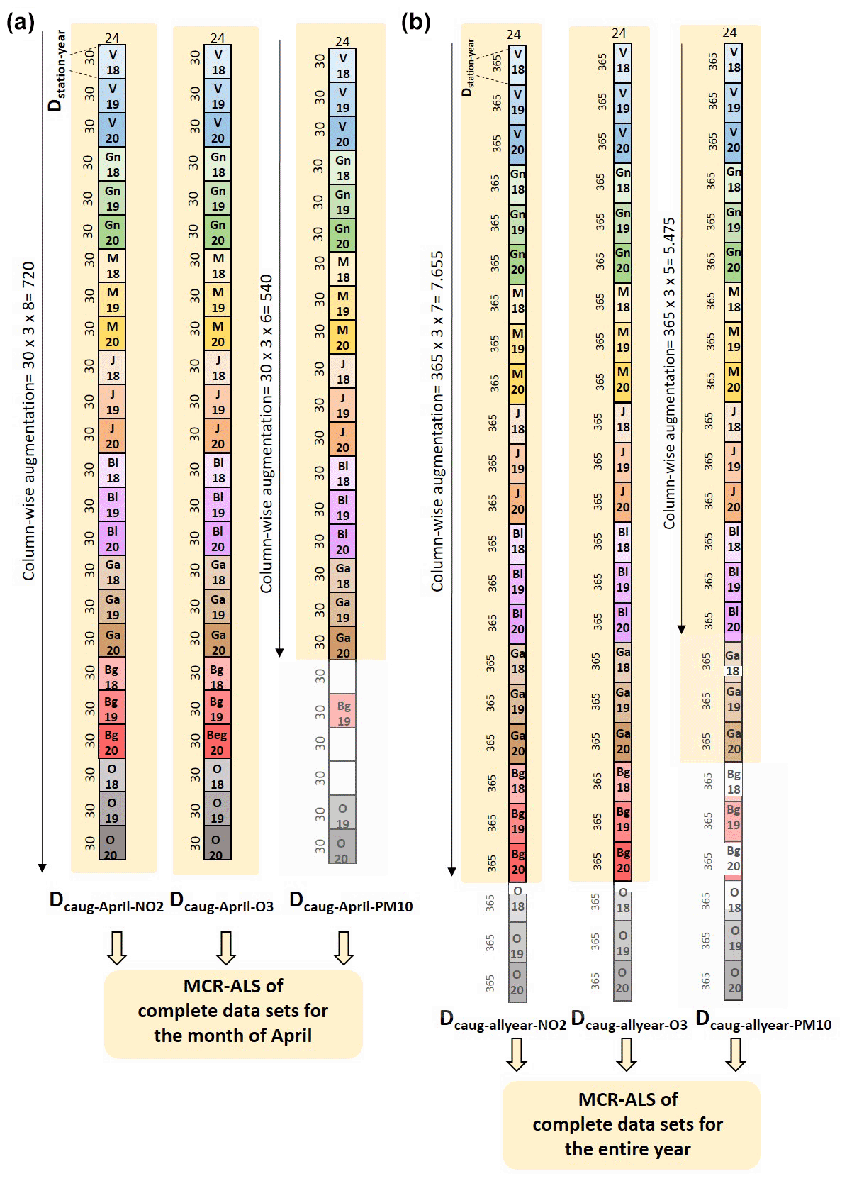
Figure 1 Data arrangement for individual analysis of completed data sets. Concentrations of NO₂, O₃, and PM₁₀ in the month of April (a) and the entire year, for one year and one station (b) can be arranged in a data matrix with the days in the rows and the 24 h measurements in the columns D_{station-April} or D_station-year. These individual data matrices are arranged in three (one per each pollutant) column-wise augmented data matrices. For the data set of April in 2018–2019–2020 (a), the augmented matrices are ${\mathbf{D}}_{{\text{caug-April-NO}}_{\mathrm{2}}}$, ${\mathbf{D}}_{{\text{caug-April-O}}_{\mathrm{3}}}$ (720, 24) and ${\mathbf{D}}_{{\text{caug-April-PM}}_{\mathrm{10}}}$ (540, 24). For the data set of the entire year in 2018–2019–2020 (b), the augmented matrices are ${\mathbf{D}}_{{\text{caug-allyear-NO}}_{\mathrm{2}}}$, ${\mathbf{D}}_{{\text{caug-allyear-O}}_{\mathrm{3}}}$ (7655, 24) and ${\mathbf{D}}_{{\text{caug-allyear-PM}}_{\mathrm{10}}}$ (5475, 24). Stations containing missing data (white gaps in the figure) are excluded for further MCR-ALS analysis (yellow-shaded area). VH: Vall d'Hebron, Grn: Granollers, Mn: Manlleu, Jun: Juneda, Bell: Bellver, Gra: Gràcia, Beg: Begur, OF: Observatori Fabra.

These 24 data matrices were then arranged using a column-wise arrangement, obtaining three augmented data matrices: ${\mathbf{D}}_{{\text{caug-allyear-NO}}_{\mathrm{2}}}$, ${\mathbf{D}}_{{\text{caug-allyear-O}}_{\mathrm{3}}}$, and ${\mathbf{D}}_{{\text{caug-allyear-PM}}_{\mathrm{10}}}$ (Fig. 1b). In this case, for the three contaminants, some data were missing (white gaps in the figure). For NO₂ and O₃, some data from the Observatori Fabra station was missing. Thus, the resulting augmented matrices, ${\mathbf{D}}_{{\text{caug-allyear-NO}}_{\mathrm{2}}}$ and ${\mathbf{D}}_{{\text{caug-allyear-O}}_{\mathrm{3}}}$, contained information of the whole year, seven stations and the 3 years ($\mathrm{365}\times \mathrm{3}\times \mathrm{7}$), resulting in 7655×24 matrices, as shown in the figure. For PM₁₀, data of three stations were missing (white gaps in the figure) corresponding to Gràcia, Begur and Observatori Fabra. Thus, in order to perform the MCR-ALS analysis, the resulting PM₁₀ column-wise augmented matrix only contained information of five stations with no missing data ($\mathrm{365}\times \mathrm{3}\times \mathrm{5}$), resulting in a 5475×24 matrix (yellow-shaded area in Fig. 1b).

Data arrangement for the simultaneous study of the three pollutants considering the whole incomplete multiblock experimental data sets is further described in Sect. 2.7.

2.4 Estimation of missing data

Estimation of missing data was used for the case when failures of stations and/or their malfunction caused the absence of measurements for a few hours or a few days. In order to estimate such missing data, the nearest-neighbor method (Peterson, 2009) (i.e., knn imputation) was used. In this study, the function mdcheck (i.e., missing data checker and infiller) of PLS Toolbox version 8.9.1 (Eigenvector Inc., WA) was utilized to perform the imputation. This function checks for missing data and infills them using a PCA model imputation from distinct algorithms. In our case, three algorithms were tested consisting of “SVD” (Singular Value Decomposition), “NIPALS” (Nonlinear Iterative Partial Least Squares) and “knn”, the latter providing the better estimation results in our case, and thus, the one that was finally used in this study.

It is important to mention that estimation of missing data was not performed in cases where the entire month was missing. For those cases, the station was not included in the MCR-ALS analysis of the complete data set. For the analysis of incomplete multiblock data sets, an especial arrangement was performed using a particular data fusion strategy, as further explained in Sect. 2.7.

2.5 MCR-ALS analysis of the experimental data

Different chemometric methods have been proposed in the literature for the analysis of environmental monitoring data. The MCR-ALS method is frequently used in spectrochemical mixture data analysis, which can also be easily extended to the analysis of environmental source apportionment data sets (Alier et al., 2011). The MCR-ALS is a flexible, soft-modeling factor analysis tool which allows for the application of natural constraints (see below), and it can be easily adapted to the analysis of complex multiway (multimode) data structures, such as three- and four-way environmental data sets using trilinear and quadrilinear model constraints (De Juan et al., 1998; Smilde et al., 2004; Malik and Tauler, 2013).

The simplest application of the MCR-ALS method is based on a bilinear model that performs the factor decomposition of a two-way data set (i.e., a data table or a data matrix). Equation (1) summarizes this bilinear model in its element-wise way, while Eq. (2) presents the same model in a matrix linear algebra format:

$$\begin{array}{}\text{(1)}& {\displaystyle }\begin{array}{rl}& d_{i,j}={\sum }_{n=\mathrm{1}}^N{x}_{i,n}{y}_{j,n}+e_{i,j}i=\mathrm{1},\mathrm{\dots }I\left(\text{days}\right),\\ & j=\mathrm{1},\mathrm{\dots }J\left(\mathrm{hours}\right)\end{array}\text{(2)}& {\displaystyle }\mathbf{D}={\mathbf{XY}}^T+\mathbf{E}.\end{array}$$

In Eq. (1), the individual data values, d_i, j elements (in this case the O₃, NO₂ or PM₁₀ concentration values measured on 1 d (i) at a particular hour (j)) are decomposed as the sum of a reduced number of contributions (components), n=1,  … N. Each one of them are defined by the product of two factors, x_i, n (scores) and y_j, n (loadings). In addition, the term e_i, j is the residual part of d_i, j, which cannot be explained by these N components and accounts as experimental noise and uncertainties. In Eq. (2), the data matrix, D, of dimensions I×J is decomposed into the scores factor matrix X (I×N) and the loadings factor matrix, Y^T (N×J). The number of components, N, is selected to explain the data variance as much as possible, while the unexplained small contributions of data variance and experimental noise are in E. Multivariate Curve Resolution (MCR; Tauler, 1995) performs the bilinear model factor decomposition shown in Eqs. (1) and (2) using an alternating least squares (ALS) algorithm under a set of constraints which reduce the extent of the bilinear model rotation ambiguities (Abdollahi and Tauler, 2011) and allow the physical identification and interpretation of the factor matrices X and Y^T, for example, the application of non-negativity constraints to the elements of the factor matrices X and Y^T (Bro and De Jong, 1997; De Juan and Tauler, 2003). Models with a different number of components can be tested and a final decision is taken considering the data fit and the shapes and reliability of the resolved profiles. The ALS algorithm also needs initial estimates of either X or Y^T factor matrices. These initial estimates can be obtained from the more “dissimilar” rows or columns of the original data matrix (Winding and Guilment, 2002). Equation (2) for D is solved iteratively, which updates the solutions (vector profiles in X and Y^T matrices) until they fit the data optimally and fulfill the proposed constraints.

In this work the MCR-ALS method has been applied, either to the individual data matrices D_{station, year} described in the previous section and in Fig. 1 for every pollutant (O₃, NO₂ or PM₁₀), at one period of time (April or full year), and at one monitoring station, or to the augmented matrices of the same three pollutants for the 3 years ($k=\mathrm{1},$… 3) simultaneously and for the different stations (l=1, … ,8), concatenated vertically in D_caug-April or D_caug-allyear (see Fig. 1). In the case of the individual data matrices described above for the period of time (April or full year), D_{station,april} or D_{station, year}, the factor (scores) matrix X will have the April or full year day profiles of the components, respectively, and the factor (loadings) matrix Y^T will have the corresponding hour profiles of these components. In the case of the column-wise augmented data matrices D_caug-April or D_caug-allyear, bilinear model Eq. (2) was extended as

$$\begin{array}{}\text{(3)}& {\mathbf{D}}_{\mathrm{caug}}={\mathbf{X}}_{\mathrm{caug}}{\mathbf{Y}}^T+{\mathbf{E}}_{\mathrm{caug}},\end{array}$$

where X_caug is now the augmented factor (scores) matrix with the augmented day profiles concatenated vertically for the different years and stations, and Y^T is the matrix of the hour profiles again, which are common for all the concatenated matrices in X_caug. During the ALS optimization of the bilinear model in Eq. (3), constraints can be also applied, and the same aspects relating to the number of components and convergence as for solving Eq. (2), are considered.

2.6 MCR-ALS analysis of the complete experimental data sets using trilinear and quadrilinear constraints

Solving Eq. (3) using bilinear MCR-ALS does not take into account the temporal and spatial structure of the data in the vertical concatenated mode, which includes the information of the day, year and station. This data structure can be considered in the trilinear and especially in the quadrilinear extensions of the bilinear models described in Eqs. (1)–(3).

The factor decomposition model given before can be extended to a three-way dataset, $\underset{\mathrm{¯}}{\mathbf{D}}$, or to a four-way data set, $\underset{=}{\mathbf{D}}$, expressed individually for every data value as given by Eqs. (4) and (5).

$$\begin{array}{}\text{(4)}& {\displaystyle }{d}_{i,j,kl}={\sum }_{n=\mathrm{1}}^N{x}_{i,n}{y}_{j,n}{z}_{kl,n}+e_{i,j,kl}\left(\text{trilinear model}\right)\text{(5)}& {\displaystyle }{d}_{i,j,k,l}={\sum }_{n=\mathrm{1}}^N{x}_{i,n}{y}_{j,n}{z}_{k,n},w_{l,n}+e_{i,j,k,l}\left(\text{quadrilinear model}\right),\end{array}$$

where $d_{i,j,kl}$ are the individual data values (concentrations of O₃, NO₂ or PM₁₀) in the four experimental data modes: the day of April or of the full year $i=\mathrm{1},\mathrm{\dots }\mathrm{30}$ or $i=\mathrm{1},\mathrm{\dots },\mathrm{365}$, the hour of the day $j=\mathrm{1},\mathrm{\dots },\mathrm{24}$, and the year–station $kl=\mathrm{1},\mathrm{\dots }\mathrm{24}$ in the case of the trilinear model, and $d_{i,j,k,l}$ has the year–station third mode separated in year $k=\mathrm{1},\mathrm{2},\mathrm{3}$, and station, $l=\mathrm{1},\mathrm{\dots },\mathrm{8}$ in the quadrilinear model. These data values are modeled as the sum of a number of components (contributions), $n=\mathrm{1},\mathrm{\dots }N$, defined by the product of three factors x_i, n, y_j, n, and z_kl, n in the case of the trilinear model and in four factors in the case of the quadrilinear model,= x_i, n, y_j, n, z_k, n and w_l, n. These factors are related to the three and four data modes, respectively (day, hour and year–station or day, hour, year and station). ${\mathbf{e}}_{i,j,kl}$ and ${\mathbf{e}}_{i,j,k,l}$ are the part of ${\mathbf{d}}_{i,j,kl}$ and ${\mathbf{d}}_{i,j,k,l}$ not explained by the contribution of these N components. These trilinear and quadrilinear models can be written in a matrix form using the decomposition of every individual D_kl data slice (every individual matrix D_kl), as shown in Eqs. (6) and (7).

$$\begin{array}{}\text{(6)}& {\displaystyle }{\mathbf{D}}_{kl}=\mathbf{X}{\mathbf{Z}}_{kl}{\mathbf{Y}}^T+{\mathbf{E}}_{kl}\left(\text{trilinear model}\right)\text{(7)}& {\displaystyle }{\mathbf{D}}_{kl}=\mathbf{X}{\mathbf{Z}}_k{\mathbf{W}}_l{\mathbf{Y}}^T+{\mathbf{E}}_{kl}\left(\mathrm{quadrilinearmodel}\right)\end{array}$$

Under the trilinear model, all individual data matrices, D_kl, (I, J) are simultaneously decomposed with the same number of components N and the same daily X (I, N) and hourly Y^T (N, J) profiles. Thus, they differ only in a diagonal matrix Z_kl (N, N), different for every one of the $kl=\mathrm{1},\mathrm{\dots },\mathrm{24}$ year–stations (year–station profiles), which gives the relative amounts of the N components in every data matrix (year–station), D_kl. These N diagonal elements of Z_kl can also be grouped in the third factor matrix Z ($K\times L,N$). Under the quadrilinear model, all individual data matrices, D_kl, (I, J) are simultaneously decomposed with the same number of components N and the same daily X (I, N) and hourly Y^T (N, J) profiles. Thus, they differ in the diagonal matrices Z_k (N, N) and W_l (N, N), which are different for every year (k) and station (l), which give the relative amounts of the N components in every data matrix D_kl, respectively. These N diagonal elements of the Z_k and W_l matrices can also be grouped in the third- and four-factor matrices Z (K, N) and W (L, N). Therefore, the proposed trilinear and quadrilinear models take advantage of the natural structure of the analyzed data sets, especially in relation to their different temporal modes (i.e., hourly, daily, yearly) and the different type of monitoring stations analyzed simultaneously. The implementation of trilinear and quadrilinear models as a constraint in the MCR-ALS method has been described in previous works (Tauler, 2021; Malik and Tauler, 2013; Alier et al., 2011). Here only a brief explanation of the implementation of the quadrilinear model constraint for the case of study is shown.

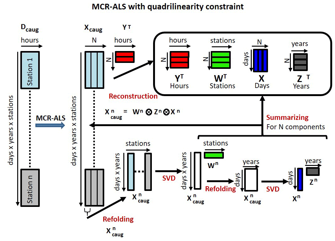
Figure 2 MCR-ALS with the quadrilinearity constraint. Graphical description of the implementation of the quadrilinearity constraint during the Alternating Least Squares (ALS) optimization. See Eqs. (4)–(7) and their explanation in the paper.

Figure 2 shows the practical implementation of the quadrilinearity constraint in the MCR-ALS analysis of the four-way data set obtained in the two types of data, when the April data of the three parameters (O₃, NO₂ and PM₁₀) were studied over the 3 years (2018–2019 and 2020), and over the different monitoring stations described above, and also for the analogous four-way data set when instead of April data, the full-year data were considered for the same years and stations.

The individual data sets with the concentrations of the three parameters (one per year and station), were arranged in the column-wise augmented data matrix D_caug of dimensions 30 (April) or 365 d × 3 years × 8 stations, giving a total number of 720 rows for April data or of 8760 rows for the full-year data, and 24 hourly measures in columns. These number of row elements is for the case of no-missing data, however they will be lowered for the cases of missing data, especially in the case of the full-year data (see previous section in missing data). The application of the quadrilinearity constraint implies that the augmented profiles of every component n, ${\mathbf{x}}_{\mathrm{aug}}^n$, having the vertically concatenated information of days × years × stations is first refolded in the data matrix ${\mathbf{X}}_{\mathrm{aug}}^n$ of dimensions 30 (April) or 365 (all year) × 3 (years) rows by 8 (stations). This augmented factor matrix is decomposed by SVD considering only the first singular component into the product of two vector profiles, one long vector profile ${\mathbf{x}}_{\mathrm{caug}}^n$ (90 or 1095×1) of the combined day–year profile by a vector profile wⁿ (8×1) describing differences among the different stations for the component n. The ${\mathbf{x}}_{\mathrm{caug}}^n$ long vector day–year profile can be further refolded in a matrix and decomposed by SVD into the product of two new vector profiles, one related to the year profile, zⁿ, and another to the day profile xⁿ, for the considered component n. In this way, for every component (contribution), the concentration of any one of the three parameters (O₃, NO₂, and PM₁₀) is decomposed in the product of four profiles, one related to the day (of April or of the whole year), xⁿ, another related to the hour of the day, yⁿ, another to the considered year, zⁿ, and another to the monitoring station, wⁿ. This factor decomposition allows a detangled interpretation of the temporal and spatial sources of variation for the observed concentrations of the three pollutants. Therefore, the application of this quadrilinearity constraint implies that for every component, the daily changes are described by the same single xⁿ vector profile which changes over the years and station by station by the corresponding scalar values in zⁿ and wⁿ. Once the three profiles in the three augmented modes, x_n, z_n and w_n, are obtained, they can be multiplied using the Kronecker product (Soloveychik and Trushin, 2016) to reconstruct the long vector profile, ${\mathbf{x}}_{\mathrm{aug}}^n$, (see Fig. 2) and rebuild the bilinear model in the next iteration of the general ALS optimization. Finally, the vector profiles for every component n in the different modes, can be grouped in the corresponding factor matrices X, Z, and W, which together with Y^T give the full quadrilinear decomposition of the four-way data set, $\underset{=}{\mathbf{D}}$. See previous works for a more detailed description of the algorithm used for the practical implementation of the quadrilinearity constraint in MCR-ALS (De Juan and Tauler, 2001; De Juan et al., 1998).

2.7 MCR-ALS simultaneous analysis of incomplete multiblock experimental data

The simultaneous analysis of the NO₂, O₃, and PM₁₀ experimental data can be done one step forward using a data fusion multiblock strategy. This would imply building a single MCR model for the whole multiset data obtained for the three pollutants, NO₂, O₃, and PM₁₀ in April or in the whole year, for the 3 years, 2018, 2019, and 2020, and for the different monitoring stations. This is expressed in the following data matrix equation (see also Fig. 3):

$$\begin{array}{}\text{(8)}& \begin{array}{rl}{\mathbf{D}}_{\mathrm{craug}}& =[{\mathbf{D}}_{{\mathrm{caugNO}}_{\mathrm{2}}},{\mathbf{D}}_{{\mathrm{caugO}}_{\mathrm{3}}},{\mathbf{D}}_{{\mathrm{caugPM}}_{\mathrm{10}}}]\\ & ={\mathbf{X}}_{\mathrm{caug}}[{\mathbf{Y}}_{{\mathrm{NO}}_{\mathrm{2}}}^T,{\mathbf{Y}}_{{\mathrm{O}}_{\mathrm{3}}}^T,{\mathbf{Y}}_{\mathrm{PM}}^T]={\mathbf{X}}_{\mathrm{caug}}{\mathbf{Y}}_{\mathrm{raug}}^T.\end{array}\end{array}$$

In this Equation the column-wise augmented data matrices, ${\mathbf{D}}_{{\mathrm{caugNO}}_{\mathrm{2}}}$, ${\mathbf{D}}_{{\mathrm{caugO}}_{\mathrm{3}}}$, and ${\mathbf{D}}_{{\mathrm{caugPM}}_{\mathrm{10}}}$ described previously (and analyzed separately by MCR-ALS with different factor decomposition models, bilinear, trilinear and quadrilinear), are now concatenated horizontally giving the new single row and column-wise super-augmented data matrix D_craug, which is decomposed in the two new augmented factor matrices, X_caug and ${\mathbf{Y}}_{\mathrm{raug}}^T$, using the MCR bilinear model and constraints, like it was described in Sect. 2.4. The resolved hour profiles for the three contaminants ${\mathbf{Y}}_{{\mathrm{NO}}_{\mathrm{2}}}^T$, ${\mathbf{Y}}_{{\mathrm{O}}_{\mathrm{3}}}^T$, and ${\mathbf{Y}}_{\mathrm{PM}}^T$ will be in the augmented rows of the new ${\mathbf{Y}}_{\mathrm{raug}}^T$. In addition, if the trilinearity/quadrilinearity constraints are applied to the columns of the resolved factor matrix X_caug as described above in Sect. 2.6 using matrix decompositions of Eqs. (6) and (7), the common day, year and station profiles will be separately recovered and analyzed.

However as previously described, April and the whole-year individual data sets were not obtained for all stations, years, and pollutants. Therefore, they could not be fitted together in a rectangular super-augmented data matrix containing all the data for all the years and stations as shown in Eq. (8) for D_craug. Some of the individual data sets were missing (see Sect. 2.3 and 2.4). In particular, in the case of April, two different data blocks could be arranged. First, the NO₂, O₃ and PM₁₀ concentrations data for 3 years and 6 stations were arranged in the complete row- and column-wise augmented April data block, DA1_craug, with 540 rows (30 d × 3 years × 6 stations) and 72 columns (24 h for NO₂ + 24 h for O₃ + 24 h for PM₁₀). Secondly, the additional NO₂ and O₃ concentration data for 3 years and 2 stations were arranged in the complete row- and column-wise augmented April data block DA2_craug with 180 rows (30 d × 3 years × 2 stations) and 48 columns (24 h for NO₂ + 24 h for O₃). These two April data blocks can be analyzed independently, but a new data set can be built concatenating the two data blocks as shown in Fig. S1, which will be reformulated and analyzed as shown in the next Equation.

$$\begin{array}{}\text{(9)}& \begin{array}{rl}& \mathbf{DA}{\mathbf{12}}_{\mathrm{craug}}=[\mathbf{DA}{\mathbf{1}}_{\mathrm{craug}};[\mathbf{DA}{\mathbf{2}}_{\mathrm{craug}},\mathbf{NaN}(\mathrm{180},\mathrm{24})\left]\right]=\\ & =\mathbf{XA}{\mathbf{12}}_{\mathrm{caug}}\mathbf{YA}{\mathbf{12}}_{\mathrm{raug}}^T=\mathbf{XA}{\mathbf{12}}_{\mathrm{caug}}[{\mathbf{Y}}_{{\mathrm{NO}}_{\mathrm{2}}},{\mathbf{Y}}_{{\mathrm{O}}_{\mathrm{3}}},{\mathbf{Y}}_{{\mathrm{PM}}_{\mathrm{10}}}]\end{array}\end{array}$$

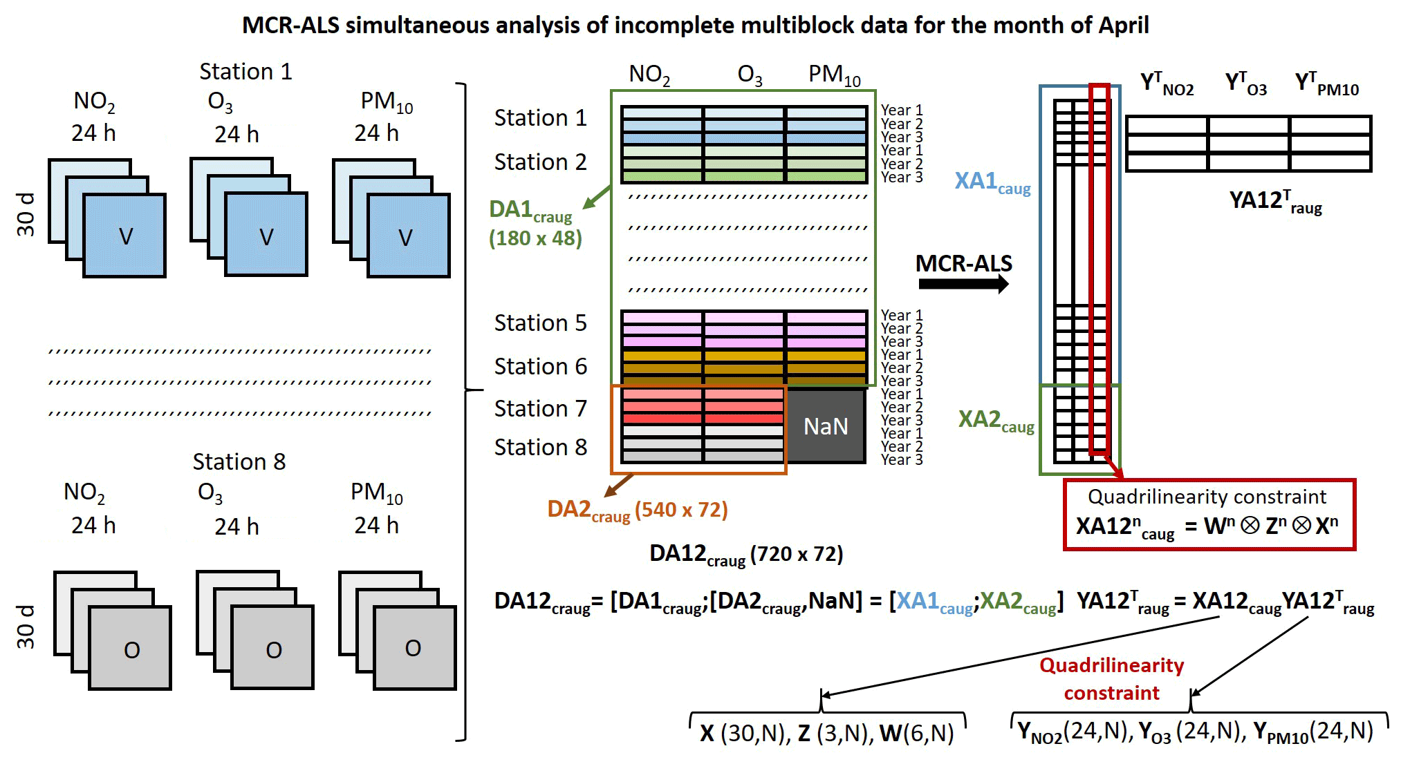
Figure 3 MCR-ALS with the quadrilinearity constraint for the simultaneous analysis of the three contaminants in the incomplete multiblock data set for the month of April. See Eq. (9) and their explanation in the paper.

This new incomplete data set DA12_craug is built using the two data blocks previously defined, DA1_craug and DA2_craug, both concatenated vertically and filling the empty data block, corresponding to the unknown concentrations of PM₁₀ for two missing stations with the NaN notation. The application of MCR-ALS to this incomplete data set is decomposed using a bilinear model (see in Fig. 3), giving the two factor matrices XA12_caug and $\mathbf{YA}{\mathbf{12}}_{\mathrm{raug}}^T$. The factor matrix XA12_caug has the column-wise augmented day × year × station profiles in its columns and the $\mathbf{YA}{\mathbf{12}}_{\mathrm{raug}}^T$ factor matrix has the row-wise augmented hour profiles for NO₂ (${\mathbf{Y}}_{{\mathrm{NO}}_{\mathrm{2}}}$), O₃ (${\mathbf{Y}}_{{\mathrm{O}}_{\mathrm{3}}}$), and PM₁₀ (${\mathbf{Y}}_{{\mathrm{PM}}_{\mathrm{10}}}$) in its rows. As previously stated, the trilinearity/quadrilinearity constraints can be applied during the ALS factor decomposition to the XA12_caug factor matrix and allow the separate recovery of the day, year and station profiles, a part of the hour profiles for NO₂, O₃ and PM₁₀obtained in $\mathbf{YA}{\mathbf{12}}_{\mathrm{raug}}^T$.

Analogous equations can be described for the NO₂, O₃, and PM₁₀ experimental data measured not only in April but during the whole year. In this case however, the two data blocks, DY1_craug and DY2_craug, will have different sizes than for the only April month data because they are for all the days of the whole year. Different data sets were missing in this case. The data for 5 stations with 5475 rows (365 d × 3 years × 5 stations) and 72 columns (24 h for NO₂ + 24 h for O₃ + 24 h for PM) is contained in DY1_craug, and DY2_craug has the additional data for 2 stations, but only for NO₂ and O₃ concentrations, with 2190 rows (365 d × 3 years × 2 stations) and 48 columns (24 h for NO₂ + 24 h for O₃) (see Fig. S2). For the whole year data, the bilinear factor decomposition can be described by the new Eq. (10):

$$\begin{array}{}\text{(10)}& \begin{array}{rl}& \mathbf{DY}{\mathbf{12}}_{\mathrm{craug}}=[\mathbf{DY}{\mathbf{1}}_{\mathrm{craug}};[\mathbf{DY}{\mathbf{2}}_{\mathrm{craug}},\mathbf{NaN}(\mathrm{2190},\mathrm{24})\left]\right]=\\ & \mathbf{XY}{\mathbf{12}}_{\mathrm{caug}}\mathbf{YY}{\mathbf{12}}_{\mathrm{raug}}^T=\mathbf{XY}{\mathbf{12}}_{\mathrm{caug}}[{\mathbf{Y}}_{{\mathrm{NO}}_{\mathrm{2}}},{\mathbf{Y}}_{{\mathrm{O}}_{\mathrm{3}}},{\mathbf{Y}}_{{\mathrm{PM}}_{\mathrm{10}}}],\end{array}\end{array}$$

where DY12_craug is now the new incomplete data set built with the two data blocks DY1_craug and DY2_craug concatenated vertically, and NaN (2190,24) is for the missing PM₁₀ concentrations during 3 years in the missing 2 stations (see Fig. S2 in the Supplement). The two factor matrices, XY12_caug and $\mathbf{YY}{\mathbf{12}}_{\mathrm{raug}}^T$, are now obtained in the bilinear decomposition of DY12_craug. The first factor matrix XY12_caug has the column-wise augmented day × year × station profiles in its columns and the second factor matrix $\mathbf{YY}{\mathbf{12}}_{\mathrm{raug}}^T$ has the hour profiles for NO₂, O₃, and PM₁₀ in its rows. Similarly, as previously stated, the trilinearity/quadrilinearity constraints applied during the ALS factor decomposition to the XY12_caug factor matrix will allow the separate recovery of the day, year and station profiles, apart from the hour profiles for NO₂ (${\mathbf{Y}}_{{\mathrm{NO}}_{\mathrm{2}}}$), O₃ (${\mathbf{Y}}_{{\mathrm{O}}_{\mathrm{3}}}$), and PM₁₀ (${\mathbf{Y}}_{{\mathrm{PM}}_{\mathrm{10}}}$) obtained in $\mathbf{YY}{\mathbf{12}}_{\mathrm{raug}}^T$. The difference with the results of April data is that now the column-wise augmented profiles in XY12_caug will have information about the 365 d of the whole year and not only for the 30 d of April. Figure S3 in the Supplement is given to graphically illustrate the bilinear model applied to the incomplete two-block data set.

In the proposed approach, missing data blocks were not included in the least squares estimations of the factor solutions (XY12_caug and [${\mathbf{Y}}_{{\mathrm{NO}}_{\mathrm{2}}}$, ${\mathbf{Y}}_{{\mathrm{O}}_{\mathrm{3}}}$, ${\mathbf{Y}}_{{\mathrm{PM}}_{\mathrm{10}}}$] in Eq. 10). On the one hand, this is an advantage of the proposed method since linear equations are only solved for the known data blocks; but on the other hand, some data regions of the factor solutions (those corresponding to the missing data blocks, NaN block in Eq. 10) will not give so much overdetermined linear equations from a least squares point of view as the other data blocks without missing values. Therefore, this can be reflected in the reliability of some parts of the factor estimations. This is an important aspect that needs further investigation and some research is pursued in this direction.

2.8 Evaluation of MCR-ALS results

The final evaluation of the MCR-ALS fitting results is performed calculating the explained data variances (R²) using Eq. (11):

$$\begin{array}{}\text{(11)}& R^{\mathrm{2}}=\mathrm{100}\times \left(\mathrm{1}-{\displaystyle \frac{{\sum }_{i=\mathrm{1}}^m{\sum }_{j=\mathrm{1}}^n{\left(d_{ij}-{\widehat{d}}_{ij}\right)}^{\mathrm{2}}}{{\sum }_{i=\mathrm{1}}^m{\sum }_{j=\mathrm{1}}^n{d}_{ij}^{\mathrm{2}}}}\right),\end{array}$$

where d_ij are the experimental predicted O₃, NO₂, or PM₁₀ concentrations, and ${\widehat{d}}_{ij}$ are the corresponding calculated values by MCR-ALS using either the bilinear (Eqs. 1–3), trilinear (Eqs. 4 and 6), or quadrilinear (Eqs. 5 and 7) models. Apart from the global fitting with the full model (all components), the explained variances can also be calculated individually for every MCR-ALS component, where now the calculated values, ${\widehat{d}}_{ij}$, only take one of the n components of the model into account. In this way, the relative importance of the different contributions can be evaluated, as well as their overlapping degree with the other contributions or components.

2.9 Software

The development platform MATLAB 9.10.0 R2021a (The MathWorks, Inc., Natick, MA, USA) was used for data analysis and visualization. The new graphical interface MCR-ALS GUI 2.0 (Malik and Tauler, 2013), freely available as a toolbox at the web address http://www.mcrals.info/ (last access: 6 July 2022), was used for bilinear and trilinear data sets. Statistics Toolbox^TM for MATLAB and PLS Toolbox 8.9.1 (Eigenvector Research Inc., Wenatchee, WA, USA) were also used in this work. A new specific MCR-ALS command line code for incomplete multiblock data sets is under final development and it can be requested from one of the authors (RT, email:roma.tauler@idaea.csic.es).

3 Results and discussion

Results of MCR-ALS will be shown separately for the analysis of the month of April and for the analysis of the entire years. In the study of the month of April, the individual analysis of the three contaminants per separate is initially performed, using only data from stations with no missing blocks (i.e., data matrices ${\mathbf{D}}_{{\text{caug-April-NO}}_{\mathrm{2}}}$, ${\mathbf{D}}_{{\text{caug-April-O}}_{\mathrm{3}}}$ and ${\mathbf{D}}_{{\text{caug-April-PM}}_{\mathrm{10}}}$, yellow-shaded area of Fig. 1a). Then, a simultaneous analysis of the three contaminants containing incomplete data is performed (i.e., data matrix D_A12craug, Fig. S1). In the study of the entire years, again the individual analysis of the three contaminants per separate is initially performed, using only data from stations with no missing blocks (i.e., data matrices ${\mathbf{D}}_{{\text{caug-allyear-NO}}_{\mathrm{2}}}$, ${\mathbf{D}}_{{\text{caug-allyear-O}}_{\mathrm{3}}}$ and ${\mathbf{D}}_{{\text{caug-allyear-PM}}_{\mathrm{10}}}$, yellow-shaded area of Fig. 1b). Then, a simultaneous analysis of the three contaminants containing incomplete data is performed (i.e., data matrix D_Y12craug, Fig. S3). In all cases the selection of the number of components and the initial estimates for MCR-ALS were performed as described in Sect. 2.5. A summary of the explained variances of the MCR-ALS analyses for the different data sets with non-negativity and either bilinear, trilinear or quadrilinear modeling, and with a different number of components is given in Table 1.

Table 1 MCR-ALS decomposition and explained variances for the different models.

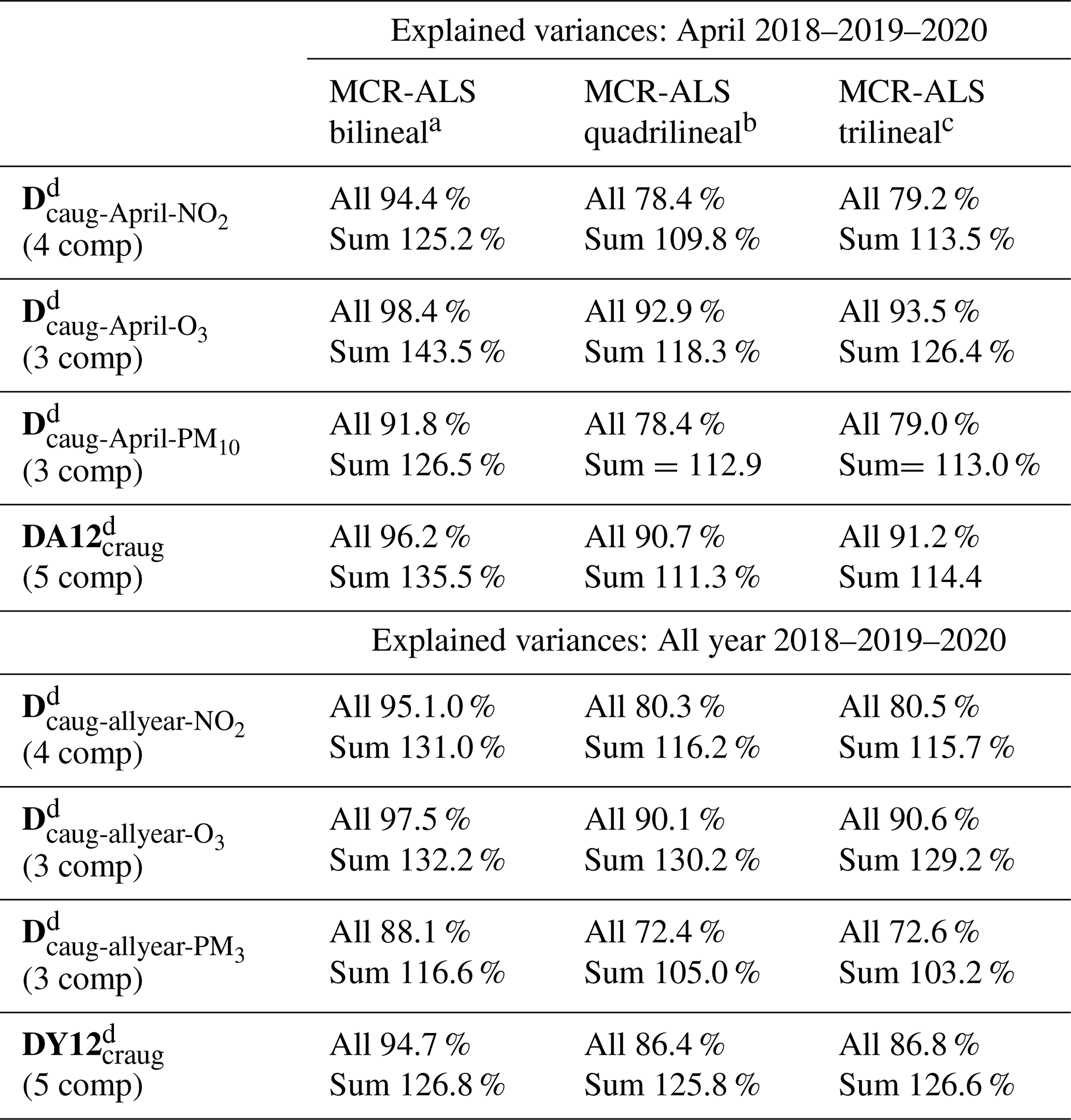
^a MCR-ALS for raw data with non-negativity constraint.
^b MCR-ALS for raw data with non-negativity and quadrilinearity constraint.
^c MCR-ALS for raw data with non-negativity and trilinearity constraint.
^d Augmented data matrices and number of components (see Fig. 1, Eqs. 3, 9 and 10, and explanation in “Data sets arrangement” section).

The MCR-ALS bilinear analysis of April data in the ${\mathbf{D}}_{{\text{caug-April-NO}}_{\mathrm{2}}}$, ${\mathbf{D}}_{{\text{caug-April-O}}_{\mathrm{3}}}$ and ${\mathbf{D}}_{{\text{caug-April-PM}}_{\mathrm{10}}}$ data matrices with non-negativity constraints explained respectively 94.40 %, 98.4 % and 91.8 % of the total variance when four, three, and three components were considered (Table 1). These values indicate the higher complexity of the NO₂ data compared to O₃ data, as will be shown also below. When the quadrilinearity constraint was applied, these values decreased to 78.4 %, 92.9 % and 78. 4 % respectively, reconfirming the less complex and more regular changes of O₃ concentrations in the 3 years at the different monitoring stations. Variances explained by the individual components are given in the figures shown below. The amount of variance overlap (also given in Table 1) in every case can be obtained by subtracting the sum of the individual variances from the variance obtained with all the components simultaneously. Again, this difference is larger in the case of NO₂. In Table 1, the variances obtained when the trilinearity constraint was applied, instead of the quadrilinearity constraint, are also given, with similar results to those obtained by both multilinear models. In the case of MCR-ALS for all-year data of the ${\mathbf{D}}_{{\text{caug-allyear-NO}}_{\mathrm{2}}}$, ${\mathbf{D}}_{{\text{caug-allyear-O}}_{\mathrm{3}}}$ and ${\mathbf{D}}_{{\text{caug-allyear-PM}}_{\mathrm{10}}}$ data matrices, rather similar results to those from April were obtained in terms of explained variances for all three types of models (see Table 1), again reflecting the higher complexity of the NO₂ data over the years and stations compared to O₃ data, and the intermediate behavior of PM₁₀ data, although the latter is more similar to the NO₂ data.

Possible correlations between NO₂, O₃, and PM₁₀ data sets during the month of April of 2018, 2019, and 2020 as well as in the eight stations were investigated using the incomplete data arrangement described in Sect. 2.7 and Fig. S1. The MCR-ALS analysis of DA12_craug with five components and with only negativity constraints gave a total explained variance of 96.2 % (Table 1). When the quadrilinearity constraint was applied, the total explained variance decreased to 90.7 % (91.2 % for the trilinear MCR-ALS model). Such a decrease of only 5 % between bilinear and quadrilinear MCR-ALS models indicated a good quadrilinear behavior of the whole system in April. The explained variances of each component individually are given below with the corresponding figures of the resolved profiles. The case of the simultaneous study of NO₂, O₃, and PM₁₀ profiles along all 3 years (i.e., 2018, 2019 and 2020) in the seven stations using the incomplete data arrangement is described in Sect. 2.7 and Fig. S3. Results using five components also indicated a rather good quadrilinear behavior of the system. A more detailed description of the profiles, describing the concentration changes of the three pollutants and of the behavior of the whole systems formed by all of them in the different stations and during the 3 years, separately for April and for the entire year, is given below.

3.1 Study of the month of April

3.1.1 NO₂ study (${\mathbf{D}}_{{\text{caug-April-NO}}_{\mathrm{2}}}$ data matrix)

In Fig. 4, from left to right, the profiles of the different modes of the four components are shown: X – day (blue), Z – year (black), W – station (green), and Y – hours (red). Component profiles in the four modes obtained by MCR-ALS when using non-negativity and quadrilinearity constraints are shown in Fig. 4.

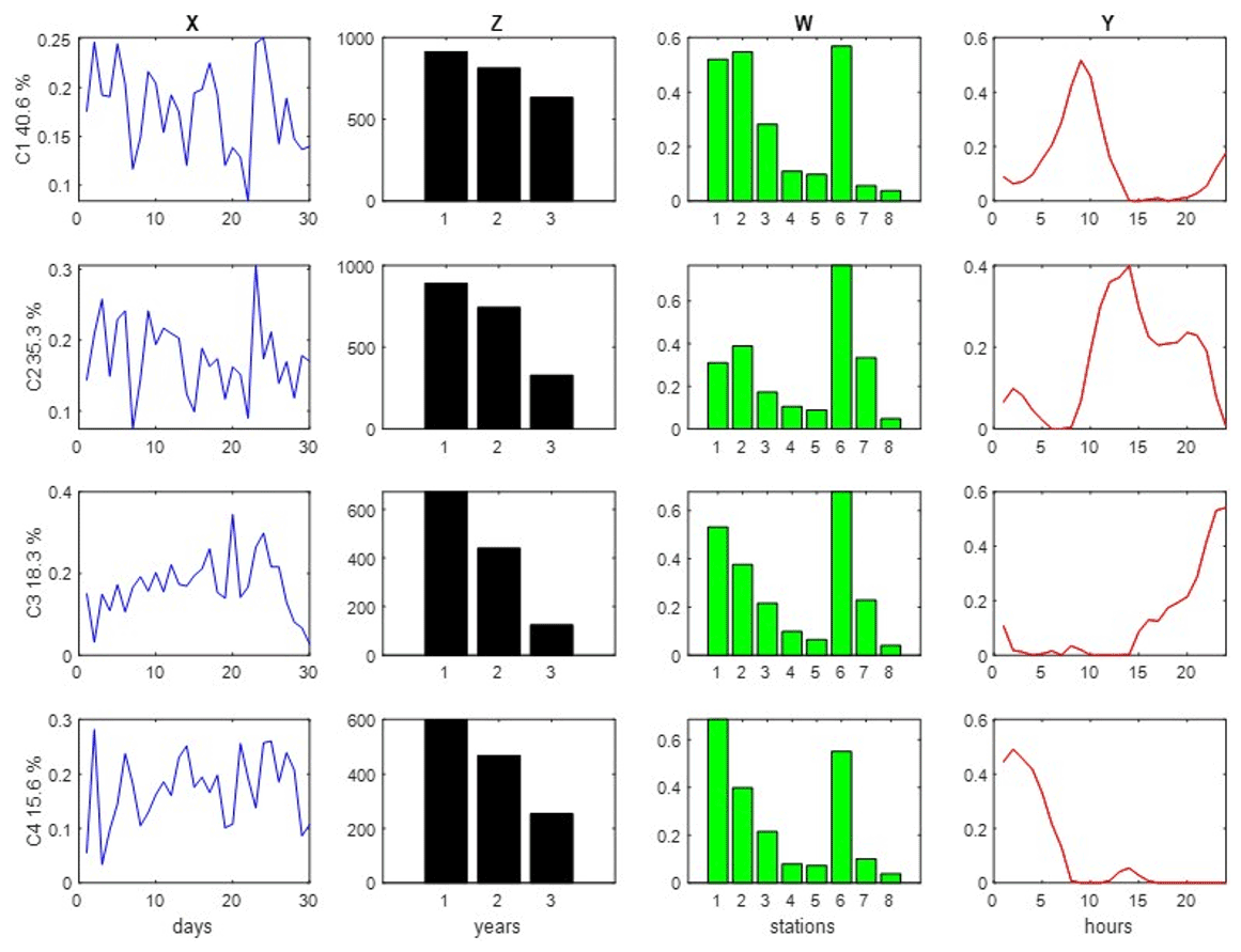
Figure 4 MCR-ALS analysis of NO₂ concentrations in the column-wise super-augmented data matrix ${\mathbf{D}}_{{\text{caug-April-NO}}_{\mathrm{2}}}$ (Eq. 3) using non-negativity and quadrilinearity constraints. Profiles of the four different data modes are given in different colors: (X) in blue – days of April; (Z) in black – year 1=2018, 2=2019 and 3=2020; (W) in green – stations 1: Vall d'Hebron, 2: Granollers, 3: Manlleu, 4: Juneda, 5: Bellver, 6: Gràcia, 7: Begur, 8: Observatori Fabra; and (Y) in red - hours of the day.

The NO₂ hour profile of the first component (C1) showed a narrow maximum between 09:00–11:00 LT (Spain, throughout) coincident with the rush-hour traffic and due to fuel combustion by vehicles. In the second component (C2) this hour profile presented a much wider peak during daily hours (10:00–20:00 LT), again potentially attributed to the combined effects of traffic emissions and O₃ formation (see below). The third component (C3) reached an hourly maximum in the late evening, approximately at 22:00 LT, whereas the fourth component (C4) showed a maximum between 00:00 and 05:00 LT, describing the NO₂ nighttime behavior. As observed in the year profiles (Z-mode), for all the components, NO₂ contributions showed a significant decrease in 2019 and even higher in 2020 with respect to 2018; the latter possibly attributed to the COVID-19 curfew and mobility restrictions. Moreover, as observed in the station profiles (W-mode), such a depletion was consequently more notorious in the three urban stations (Vall d'Hebron (1), Granollers (2) and Gràcia (6)), which were the stations with higher NO₂ concentration levels. Considering that the principal emission source of NO₂ is traffic, it is reasonable that the four MCR-ALS resolved components evidenced a decline in the year-mode, corresponding to a diminution in April 2020 (under the strictest lockdown), compared to 2019 (under no pandemic) and 2018 (under no pandemic and no other traffic restrictions in Barcelona, such as the low emission zones (LEZs; LEZ – Àrea Metropolitana de Barcelona, 2020). Moreover, as stated in a previous study of the authors (Gorrochategui et al., 2021), in April 2020 a historical record of rainfall was registered in the control site of Observatory Fabra (8). Therefore, the highly rainy conditions of April 2020 favored the cleansing of the atmosphere, including NO₂ gases. Finally, the day profiles (X-mode) for the different components did not show any particular pattern for the different days of the month.

3.1.2 O₃ study (${\mathbf{D}}_{{\text{caug-April-O}}_{\mathrm{3}}}$ data matrix)

Profiles obtained by MCR-ALS for the three components using non-negativity and quadrilinearity constraints are shown in Fig. 5. The MCR-ALS hourly (Y-mode) resolved profiles of the first component (C1) showed a maximum between 14:00–22:00 LT, due to the cumulative solar radiation. There was practically no difference in this component among stations, years or the days of the month. The MCR-ALS hourly resolved profile of the second component (C2) showed a different O₃ profile, corresponding to the concentration at night. As observed in the W-mode, O₃ concentration at night was higher in the rural station of Begur (7) and in the control site Observatori Fabra (8). The latter is emplaced in Collserola mountain and only receives some impact from Barcelona's city. The higher nightly O₃ concentration observed in these stations is due to the fact that in inner rural areas, as well as in the control site, with low anthropogenic activities, the titration effect (i.e., O₃ destruction under no solar radiation) produced by NO₂ emissions is generally not observed, resulting in higher average O₃ concentrations than in urban areas. Finally, the third component (C3) also showed a maximum between 16:00–21:00 LT, similar to the behavior described by C1, but narrower and with a pattern among stations different to C1.

Figure 5 MCR-ALS analysis of O₃ concentrations in the column-wise super-augmented data matrix ${\mathbf{D}}_{{\text{caug-April-O}}_{\mathrm{3}}}$ (Eq. 3) using non-negativity and quadrilinearity constraints. Profiles of the four different data modes are given in different colors: (X) in blue – days of April; (Z) in black – year 1=2018, 2=2019 and 3=2020; (W) in green – stations 1: Vall d'Hebron, 2: Granollers, 3: Manlleu, 4: Juneda, 5: Bellver, 6: Gràcia, 7: Begur, 8: Observatori Fabra; and (Y) in red – hours of the day.

3.1.3 PM₁₀ study (${\mathbf{D}}_{{\text{caug-April-PM}}_{\mathrm{10}}}$ data matrix)

Profiles obtained by MCR-ALS for these three components using non-negativity and quadrilinearity constraints are shown in Fig. 6. The MCR-ALS hourly resolved profiles in the Y-mode for the three resolved components indicated a wide maximum between 00:00–15:00 LT (C1), between 15:00–22:00 LT (C2), and between 10:00–20:00 LT (C3). As observed in the year profile (Z-mode), the PM₁₀ contribution decreased in 2019 but most significantly in 2020, probably due to the COVID-19 lockdown period. This same behavior was observed for NO₂ (Fig. 4), and it is due to the fact that among the PM₁₀ sources, traffic should also be included. Moreover, such a depletion was more evident in the urban stations profile (W-mode) of Vall d'Hebron (1), Granollers (2), and Gràcia (6).

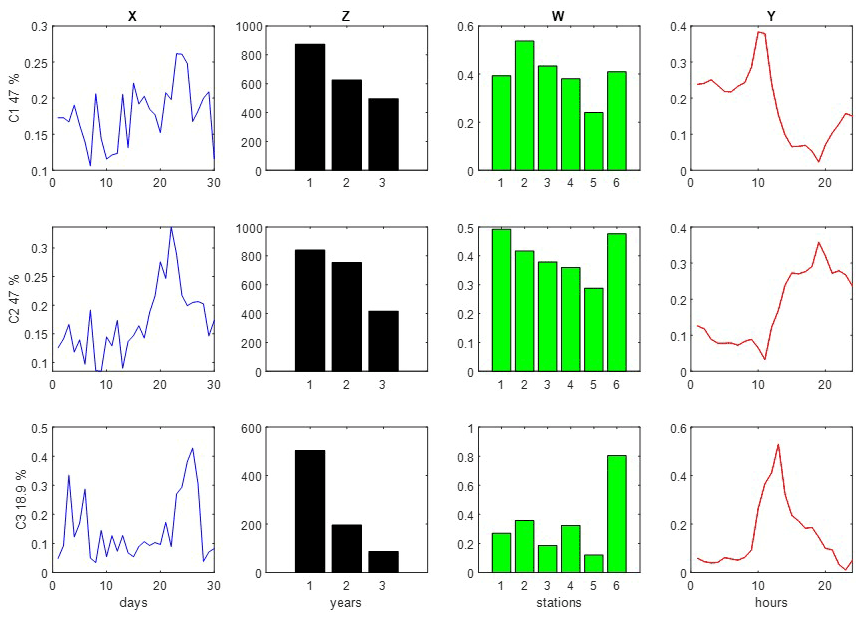
Figure 6 MCR-ALS analysis of PM₁₀ concentrations in the column-wise super-augmented data matrix ${\mathbf{D}}_{{\text{caug-April-PM}}_{\mathrm{10}}}$ (Eq. 3) using non-negativity and quadrilinearity constraints. Profiles of the four different data modes are given in different colors: (X) in blue – days of April; (Z) in black – year 1=2018, 2=2019 and 3=2020; (W) in green – stations 1: Vall d'Hebron, 2: Granollers, 3: Manlleu, 4: Juneda, 5: Bellver, 6: Gràcia; and (Y) in red – hours of the day.

3.1.4 NO₂, O₃ and PM₁₀ simultaneous study (DA12_craug data matrix)

The MCR-ALS resolved profiles of the DA12_craug data matrices (see “Materials and methods” Sect. 2.7) are given in Fig. 7. Results obtained for the hour profiles (Y-mode, in red) of the three pollutants, NO₂, O₃ and PM₁₀, are overlaid in the same plot with the same time axis. In this way, possible correlations among the different pollutants can be better explored in these plots. Profiles of components 1 (C1) and 2 (C2) mostly described the O₃ pollution: C1 hour profile showed an O₃ daytime profile with a wide maximum between 12:00–22:00 LT and C2 described the O₃ nighttime profile, again with a large maximum between 00:00–10:00 LT. Component 3 (C3) described both PM₁₀ and NO₂ correlated pollution sources, with PM₁₀ having the highest contribution. The correlation between NO₂ and PM₁₀ can be due to the common sources of these contaminants (i.e., traffic and industry). Component 4 (C4) described the nighttime profile of NO₂ and lastly, component 5 (C5) showed the daily NO₂ profile with two maxima, one in the morning (10:00–15:00 LT) and another in the late evening (20:00–22:00 LT), probably attributed to the traffic. From the year profiles in Z-mode, the evolution of the pollution in the month of April along 2018, 2019 and 2020 could be elucidated. Interestingly, for C1 and C2 (mostly describing O₃ pollution), the variation remained rather constant for the month of April during these 3 years. Moreover, the variation among stations in the profiles (W-mode) for the first two components was very little. Only in C2, the stations of Begur (7) and Observatori Fabra (8) showed a higher O₃ contribution, probably due to the lower titration effect produced in rural areas and in the Observatori Fabra control site (8), as previously observed in the individual MCR-ALS analysis of O₃ data. In contrast, the variation among stations and among years was more significant for the rest of the components (C3–C5), mainly describing NO₂ and PM₁₀ contamination. As observed in Z-modes, contamination by NO₂ and PM₁₀ was lower in 2019 and even lower in 2020. Considering that the most important source of NO₂ is traffic, the decrease in 2019 can be explained by the implementation of LEZs (LEZ – Àrea Metropolitana de Barcelona, 2020) in Barcelona, as a traffic restriction policy, first implemented in 2017 and finally put into permanent effect on 1 January 2020. However, the decrease observed in 2020 might be mostly associated with the COVID-19 lockdown restrictions, being April 2020, the time when the strictest confinement was declared in Catalonia (Gobierno de España, 2020a). Regarding the variation among stations, C3–C5 showed a higher NO₂ and PM₁₀ contribution in three urban stations (Vall d'Hebron (1), Granollers (2), and Gràcia (6)), which is in accordance with the higher traffic density registered on these sites. The results observed for C3–C5 regarding NO₂ and PM₁₀ pollution were in concordance with those of their respective individual models, evidencing the good performance of the MCR-ALS simultaneous analysis of the incomplete multiblock data sets and the confirmation of the reliability of the proposed approach.

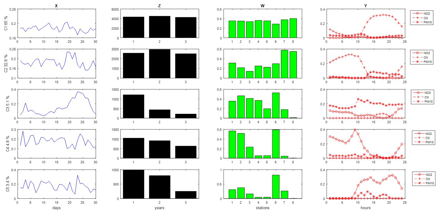
Figure 7 MCR-ALS analysis of NO₂, O₃ and PM₁₀ concentrations in the column-wise super-augmented incomplete April data matrix DA12_craug (see Eq. 9) using non-negativity and quadrilinearity constraints. Profiles of the four different data modes are given in different colors: (X) in blue – days of the year; (Z) in black – year 1=2018, 2=2019 and 3=2020; (W) in green – stations 1: Vall d'Hebron, 2: Granollers, 3: Manlleu, 4: Juneda, 5: Bellver, 6: Gràcia, 7: Begur, 8: Observatori Fabra; and (Y) in red – hours of the day.

3.2 Study of the entire years

3.2.1 NO₂ study (${\mathbf{D}}_{{\text{caug-allyear-NO}}_{\mathrm{2}}}$ data matrix)

Profiles obtained by MCR-ALS using non-negativity and quadrilinearity constraints are shown in Fig. S4. The hour profiles of the four resolved components in the analysis of the entire years were similar to those obtained in the analysis of the month of April: C1 hour profile in April's model was equivalent to C3 hour profile in all years' model, and C2 and C4 hour profiles were equivalent in both models. Also, the diminution observed in Z-mode profile in 2019, and to a greater extent in 2020, in the month of April was also produced when analyzing all the years, but to a lesser extent. This might be due to the fact that the traffic restriction policies were mostly implemented during the strictest confinement (from 14 March to 4 May in Catalonia) and were gradually removed in the de-escalation phases (Gorrochategui et al., 2021). Also, the extraordinary rainy conditions registered in April 2020 (Gorrochategui et al., 2021) were not registered for the rest of the months, making the NO₂ depletion less noticeable in the analysis of the entire year. Regarding stations, the ones showing the higher contribution were the same three urban stations (i.e., Vall d'Hebron (1), Granollers (2) and Gràcia (6)) observed in the study of the month of April. In the day-of-year X-mode, some seasonal tendencies can be observed in C1 and C2, with their lower intensities in the middle of the profile corresponding to the warmer seasons with higher sunlight radiation and higher NO₂ depletion due to the photochemical reaction to form O₃. The year profiles in C3 and C4 did not show major differences over the years.

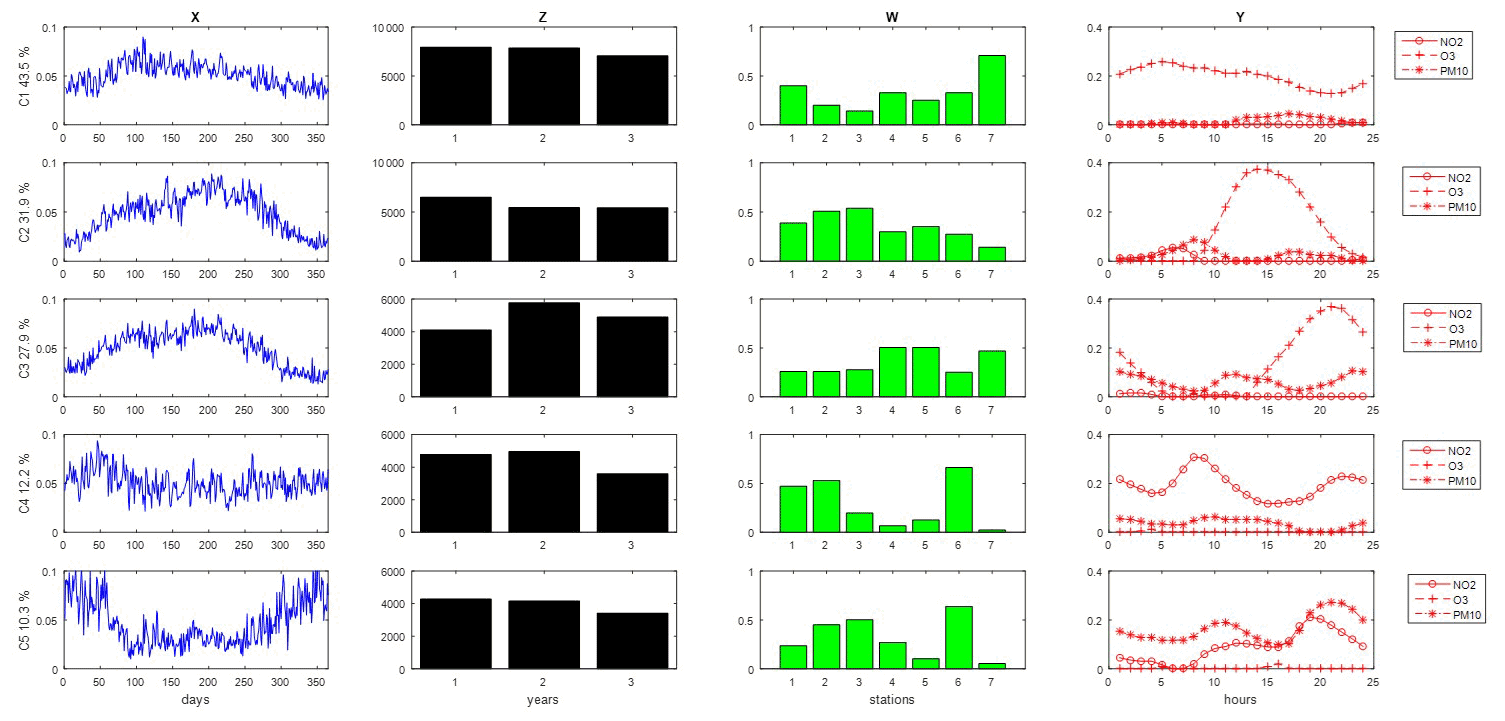
Figure 8 MCR-ALS results of the simultaneous analysis of NO₂, O₃ and PM₁₀ for the entire years (incomplete super-augmented data matrix D_Y12craug) using non-negativity and quadrilinearity constraints. Profiles of the four different data modes are given in different colors: (X) in blue – days of the month April; (Z) in black – year; (W) in green – stations; and (Y) in red – hours. In the Y-mode, the hour profiles of the three contaminants are overlapped. The different stations are indicated as 1: Vall d'Hebron, 2: Granollers, 3: Manlleu, 4: Juneda, 5: Bellver, 6: Gràcia, 7: Begur.

3.2.2 O₃ study (${\mathbf{D}}_{{\text{caug-allyear-O}}_{\mathrm{3}}}$ data matrix)

Only few differences between the analysis of the entire years versus that of the month of April were observed in the inter-year Z-mode (Fig. S5). Component 2 in all years' model, corresponding to a late evening peak of O₃, suffered a slightly significant increase in 2019 and 2020 with respect to 2018, which was not observed in the analysis of the month of April. Such increments can be explained by the reduction of the titration effect, which was a little higher when considering the entire years. The diminution of C3 in 2019 and in 2020 was also more evident when analyzing the entire years. In this case, this component was associated with the daily maximum of O₃, coincident with the sunlight hours and summer and spring seasons, when the photochemical reactions with NO_x take place to form O₃. The reason why the changes in O₃ were more evident when considering the all-year analysis instead of just the month of April, as opposed to what happened with NO₂, might be due to the fact that despite the traffic restrictions being gradually removed in the de-escalation phases, the curfew policies remained, causing a potential cumulative suppression of the titration effect.

3.2.3 PM₁₀ study (${\mathbf{D}}_{{\text{caug-allyear-PM}}_{\mathrm{10}}}$ data matrix)

As with NO₂ and O₃, the profiles of the components in the MCR-ALS analysis of PM₁₀ of the all years' model were similar to those obtained in the analysis of the month of April (Fig. S6). The hour profiles of C1 and C3 in April's model were equivalent to that of C3 and C1 in all years' model, respectively, and C2 described the same PM₁₀ profile in both models. Also, the diminution observed in 2019 and to a greater extent in 2020 in the month of April was also produced when analyzing all the years, but to a lesser extent, as stated for NO₂. Moreover, the meteorological stations with higher contribution in the model were the same as in the model of April, except for Manlleu (3), which showed a significant contribution in C2 of this model for the first time when the entire years' PM₁₀ data were investigated.

3.2.4 NO₂, O₃ and PM₁₀ simultaneous study (DY12_craug data matrix)

The MCR-ALS resolved profiles of DY12_craug are given in Fig. 8. As observed in the Y-mode profiles, C1 and C2 mostly described O₃ pollution: C1 showed an O₃ profile with little daily variation whereas C2 described a wide O₃ maximum between 14:00–20:00 LT. Moreover, the seasonal trend of C2 (X-mode) showed a wide maximum, coincident with the solar radiation registered in summer and spring months. The C2 was higher in the urban stations and lower in the rural station of Begur (7), which could indicate that such O₃ resulted from the photochemical reaction among NO_x in the presence of sunlight in highly transited areas. The nighttime profile of O₃ was clearly showed by C3, with a wide maxim between 17:00–00:00 LT. Interestingly, C3 was the only component to clearly show an increase in 2019 and 2020 with respect to 2018. As explained in the individual model, such an increase is due to the diminution of the titration effect. The NO₂ profile is described in C4, with a first maximum between 09:00–12:00 LT and a second but lower maximum in the late evening (20:00–00:00 LT). Component 5 described the simultaneous contribution of NO₂ and PM₁₀, with a higher contribution of PM₁₀, also having the same two-maxima profile observed in C5 for NO₂. Interestingly, both C5 and C6 presented maximums in the urban stations (Vall d'Hebron (1), Granollers (2), and Gràcia (6)), and a decrease in 2020, due to the traffic diminution registered during the COVID-19 lockdown period.

4 Conclusions

The MCR-ALS method with quadrilinearity constraints has demonstrated to be a powerful tool to resolve the principal contamination profiles of four-way environmental data sets, even when containing missing data blocks. The main advantage provided by the use of quadrilinearity constraints is the better and easier interpretability of the profiles, which appear more condensed and concise.

In this study, resolved MCR profiles using quadrilinearity constraints have been shown to adequately describe the different patterns and evolution of NO₂, O₃, and PM₁₀ contamination during the different hours of the day, during the different days (hourly and daily variations) for the two periods of time evaluated: the month of April versus the entire year for 2018, 2019 and 2020. For each period of time studied, the individual models of the contaminants together with their simultaneous analysis have been performed.

The simultaneous analysis of the incomplete multiblock data sets allowed the exploration of the potential correlations among the three contaminants, which was easily interpretable with the representation of overlapped hour profiles of NO₂, O₃ and PM₁₀. Interestingly, both in the study of the month of April and the study of the entire years, the simultaneous analysis of the three contaminants evidenced a correlation between NO₂ and PM₁₀, due to their common pollution sources (i.e., traffic and industry). Moreover, the profiles of these two contaminants showed an inter-year decrease, due to the introduction of LEZs (LEZ – Àrea Metropolitana de Barcelona, 2020) in 2019 and due to the COVID-19 lockdown restrictions as well as the high amount of rainfall registered in April 2020 (Gobierno de España, 2020b). Such a decrease was consistently higher in the three most transited urban stations studied: Vall d'Hebron, Granollers and Gràcia.

On the other hand, MCR-ALS O₃ profiles, both in individual and simultaneous models, presented an opposite inter-year trend, especially when analyzing the entire years. Globally, O₃ profiles showed an increase in 2019 and in 2020 with respect to 2018, which can be attributed to the diminution of the titration effect linked to the lockdown and curfew restrictions. Such an effect was more evident in inner rural areas and in the control site (i.e., Begur and Observatori Fabra), where the amount of NO_x necessary to react with O₃ and to produce its suppression is lower compared to urban areas due to the smaller traffic density and industrial activity.

Overall, this work contributes to the better knowledge of the evolution of NO₂, O₃ and PM₁₀ contamination in eight rural and urban areas of Catalonia during the 2 years before the COVID-19 (i.e., 2018 and 2019) and the year of the pandemic itself (i.e., 2020). The work also highlights (a) the capacity of MCR-ALS with quadrilinearity constraints to perform simultaneous analysis of different contamination sources to study potential correlations among them and (b) the good performance of this approach in the analysis of complex four-way environmental data sets containing missing data blocks,providing concise and easily interpretable results.