the Creative Commons Attribution 4.0 License.
the Creative Commons Attribution 4.0 License.
 | 19 Jan 2022
A single-peak-structured solar cycle signal in stratospheric ozone based on Microwave Limb Sounder observations and model simulations
Martyn P. Chipperfield
Wuhu Feng
Ryan Hossaini
Graham W. Mann
Michelle L. Santee
Mark Weber
Until now our understanding of the 11-year solar cycle signal (SCS) in stratospheric ozone has been largely based on high-quality but sparse ozone profiles from the Stratospheric Aerosol and Gas Experiment (SAGE) II or coarsely resolved ozone profiles from the nadir-viewing Solar Backscatter Ultraviolet Radiometer (SBUV) satellite instruments. Here, we analyse 16 years (2005–2020) of ozone profile measurements from the Microwave Limb Sounder (MLS) instrument on the Aura satellite to estimate the 11-year SCS in stratospheric ozone. Our analysis of Aura-MLS data suggests a single-peak-structured SCS profile (about 3 % near 4 hPa or 40 km) in tropical stratospheric ozone, which is significantly different to the SAGE II and SBUV-based double-peak-structured SCS. We also find that MLS-observed ozone variations are more consistent with ozone from our control model simulation that uses Naval Research Laboratory (NRL) v2 solar fluxes. However, in the lowermost stratosphere modelled ozone shows a negligible SCS compared to about 1 % in Aura-MLS data. An ensemble of ordinary least squares (OLS) and three regularised (lasso, ridge and elastic net) linear regression models confirms the robustness of the estimated SCS. In addition, our analysis of MLS and model simulations shows a large SCS in the Antarctic lower stratosphere that was not seen in earlier studies. We also analyse chemical transport model simulations with alternative solar flux data. We find that in the upper (and middle) stratosphere the model simulation with Solar Radiation and Climate Experiment (SORCE) satellite solar fluxes is also consistent with the MLS-derived SCS and agrees well with the control simulation and one which uses Spectral and Total Irradiance Reconstructions (SATIRE) solar fluxes. Hence, our model simulation suggests that with recent adjustments and corrections, SORCE data can be used to analyse effects of solar flux variations. Furthermore, analysis of a simulation with fixed solar fluxes and one with fixed (annually repeating) meteorology confirms that the implicit dynamical SCS in the (re)analysis data used to force the model is not enough to simulate the observed SCS in the middle and upper stratospheric ozone. Finally, we argue that the overall significantly different SCS compared to previous estimates might be due to a combination of different factors such as much denser MLS measurements, almost linear stratospheric chlorine loading changes over the analysis period, variations in the stratospheric dynamics as well as relatively unperturbed stratospheric aerosol layer that might have influenced earlier analyses.
- Article
(6831 KB) - Full-text XML
-
Supplement
(4246 KB) - BibTeX
- EndNote


Changes in solar irradiance over the 11-year cycle are an important external forcing to the climate system. As the largest changes occur at shorter wavelengths, such as the ultra-violet (UV) part of the solar spectrum, detecting related changes in stratospheric ozone is an obvious approach to improve our understanding of solar–climate interactions (e.g. Gray et al., 2010). Increased UV radiation during solar maximum enhances photolysis of oxygen at shorter UV wavelengths leading to ozone production, while at longer UV wavelengths enhanced ozone photolysis leads to net ozone loss through increased concentrations of atomic oxygen (Haigh, 1994).
Though many chemical models have suggested a single-peak-structured solar cycle signal (SCS) in stratospheric ozone (e.g. SPARC, 2010, chap. 10), observation-based estimates differ widely. Chandra (1984) performed an initial attempt to estimate SCS using satellite-derived stratospheric ozone profiles from Nimbus-4 Backscatter Ultra-Violet (BUV) radiometer data for the 1970–1976 time period. Their analysis suggested up to 12 % decrease in upper stratospheric ozone from solar maximum to solar minimum. Later, Hood et al. (1993) analysed 11.5 years (January 1979 to June 1990) of Nimbus-7 Solar BUV (SBUV) data and suggested that the upper stratospheric SCS is significantly smaller than the earlier estimate (about 8 %). Chandra and McPeters (1994), Fleming et al. (1995), and McCormack and Hood (1996) also analysed about 15 years (1979–1993) of SBUV data to report a SCS of about 6 %–8 % near 2 hPa, and a minimum response in the mid-stratosphere. Similarly, Chandra et al. (1996) found that upper stratosphere ozone profiles from the Microwave Limb Sounder (MLS) on board the Upper Atmospheric Research Satellite (UARS) displayed a similar magnitude of ozone change, which is about 5 % UV decrease (averaged between 200–205 nm) during the declining phase of solar cycle 22, which led to about 2 %–4 % ozone decrease in the upper stratosphere. In contrast, Wang et al. (1996) analysed Stratospheric Aerosol and Gas Experiment (SAGE) I and SAGE II ozone profiles (1979–1991) to find an almost negligible SCS in the upper stratosphere.
With the successful implementation of the Montreal Protocol, some satellite data were able to detect decreases in the upper stratospheric chlorine loading. Hence, some studies such as Newchurch et al. (2003) analysed SAGE I/II (1979–2003) and Halogen Occultation Experiment (HALOE, 1991–2003) data to suggest early signs of ozone recovery by the year 2000 in upper stratospheric ozone. However, Steinbrecht et al. (2004) analysed mid-latitude lidar-radar profiles (1987–2003) and argued that increased solar activity might have been responsible for a sudden increase in upper stratospheric ozone after the year 2000.
Later, Soukharev and Hood (2006) analysed 25 years of SBUV/SBUV2 (1979–2003) ozone profiles to show a minimum SCS in the middle stratosphere and up to 2 % SCS in the upper stratosphere. In contrast to Wang et al. (1996), their analysis of SAGE II data (1985–2003) showed up to 4 % SCS in the upper stratosphere but HALOE (1992–2003) data indicated opposite trends of about −2 % SCS in the middle stratosphere. In contrast, Remsberg (2008) and Remsberg and Lingenfelser (2010) also analysed HALOE and SAGE II ozone profiles for the HALOE time period (1992–2005) to show first and second peaks near 32 km (5 hPa) and 50 km (0.5 hPa), respectively. Recently, Dhomse et al. (2016) and Maycock et al. (2016) analysed updated SAGE V7.0 ozone profiles to show a significantly reduced SCS in the upper stratosphere. Both of those studies also noted that the SCS structure is altered significantly if the analysis is performed in mixing ratio units rather than native number density units. Recently, Ball et al. (2019) analysed updated BAyeSian Integrated and Consolidated (BASIC V2) data (1984–2016) that also showed a double-peak-structured SCS with primary peak near 35 km and secondary peak near 24 km.
Though most of the observation-based studies suggested a double-peak-structured SCS, initial 2-D model studies (Garcia et al., 1984; Brasseur, 1993; Huang and Brasseur, 1993; Fleming et al., 1995) could simulate only a single-peak-structured SCS in the middle stratosphere. The lack of double-peak structure in the chemical models was attributed to discrepancies in the 2-D transport. Later, Dhomse et al. (2011) used a 3-D chemical transport model (CTM) to successfully simulate a double-peak-structured SCS over 1979–2005 time period. However, most free-running 3-D chemistry-climate models (CCMs) also simulate only a single-peak-structured SCS in the tropical middle stratosphere (SPARC, 2010, Fig. 8.11). The inability of CCMs to simulate a SBUV/SAGE-type SCS is generally attributed to inadequate or missing representation of key dynamical processes such as the Quasi-Biennial Oscillation (QBO), El Niño–Southern Oscillation, changes in the meridional circulation and stratospheric aerosol-induced chemical/dynamical changes following the El Chichón and Mount Pinatubo volcanic eruptions (e.g. Lee and Smith, 2003; Smith and Matthes, 2008; Dhomse et al., 2011, 2015, 2020; Chiodo et al., 2014).
Another important factor has been large uncertainties in solar flux measurements (e.g. Ermolli et al., 2013). Most model simulations are forced with solar irradiance variability from (semi)empirical models such as Naval Research Laboratory (NRL) and SATIRE (e.g. Lean, 2000; Krivova et al., 2010; Yeo et al., 2014; Coddington et al., 2016) that are in general good agreement with many solar observations (Lean and DeLand, 2012; Coddington et al., 2019). However, with the launch of the Solar Radiation and Climate Experiment (SORCE) satellite in January 2003, high-resolution solar irradiance measurements suggested significantly different UV variability (Harder et al., 2009). Using SORCE measurements some modelling studies (Haigh et al., 2010; Merkel et al., 2011; Swartz et al., 2012) suggested a negative SCS in the upper stratosphere–lower mesosphere (US–LM). These studies included analysis of few years of MLS and Sounding of the Atmosphere using Broadband Emission Radiometry (SABER) datasets to show consistent changes in the observed ozone profiles. In contrast, Dhomse et al. (2013) used the same SORCE fluxes and found that SORCE-based solar spectral irradiance (SSI) changes were not enough to explain observed ozone changes. Other studies soon confirmed that initial versions of SORCE data overestimated UV variability (e.g. Ermolli et al., 2013; Haberreiter et al., 2017).
An important aspect of solar flux variability has been differences in terms of sunspot numbers (SSNs) and their durations over different solar cycles (e.g. Chapman et al., 2020). For example, SILSO World Data Center (2021) data clearly show significantly different maximum monthly SSNs during solar cycle 21 (≈ 210), 22 (≈ 200), 23 (≈ 150) and 24 (≈ 100). This clearly highlights that recent solar cycles had values about 200 reducing to 150 and 100 during solar cycles 23 and 24, respectively. This indicates that solar flux variability (solar maxima minus solar minima) would have different characteristics over different solar cycles. Hence, Dhomse et al. (2015) analysed model and satellite datasets over different time periods to show differences in SCS magnitudes depending on analysis period such as 1979–2013 (SBUV), 1984–2005 (SAGE), 1992–2005 (HALOE) and 2004–2013 (MLS). However, for each analysis period, both satellite and model-simulated ozone profiles showed a double-peak-structured SCS in the tropical stratospheric ozone. It is important to note that the SBUV, SAGE II and HALOE analysis periods include years where the stratospheric aerosol layer was strongly perturbed by El Chichón and/or Mount Pinatubo volcanic eruptions.
Overall, there is still a large uncertainty in our understanding of the true nature of the ozone SCS profile as most estimates rely on sparsely sampled solar occultation instruments (SAGE II, HALOE) or SBUV data with poor vertical resolution and may depend on the time period considered (e.g. Remsberg and Lingenfelser, 2010; Dhomse et al., 2015) . Here, we analyse 16 years (2005–2020) of updated, high-quality and densely sampled MLS ozone profiles to quantify the stratospheric SCS. We also use the TOMCAT/SLIMCAT 3-D CTM to analyse effects of different updated solar fluxes. Finally, we present the estimated SCS profile using different linear regression models such as ordinary least squares (OLS), lasso, ridge, and elastic net. The model setup and satellite data used here are described in Sect. 2 followed by details of our regression model in Sect. 3. Key results are discussed in Sect. 4.
We have performed simulations with the TOMCAT three-dimensional CTM (Chipperfield, 2006; Chipperfield et al., 2017) for the 2004–2020 time period. The model setup is similar to the control simulation used in our recent studies (e.g. Dhomse et al., 2019; Feng et al., 2021; Weber et al., 2021). Briefly, the model contains a detailed description of stratospheric chemistry and is forced using European Centre for Medium-Range Weather Forecasts fifth-generation reanalysis (ERA-5) meteorological fields (Hersbach et al., 2020). Model simulations are performed at 2.8∘ × 2.8∘ horizontal resolution with 32 levels ranging from the surface to ∼ 60 km. Surface concentrations of ozone depleting substances (ODSs) and greenhouse gases are from Engel et al. (2018b). Stratospheric sulfate aerosol surface density (SAD) data are from ftp://iacftp.ethz.ch/pub_read/luo/CMIP6/ (last access: August 2021) and have been updated since Dhomse et al. (2015) to extend until 2018. As the equivalent SAD values are not yet released for later years, we use monthly averaged SAD (1996–2005) for 2019 and 2020. Thus, our analysis will miss the impact on ozone of SAD changes following the Raikoke and Ulawun eruptions in June 2019. The model also includes contributions from four chlorinated very short-lived substances (CH2Cl2, CHCl3, C2Cl4, and C2H4Cl2) as described in Hossaini et al. (2017, 2019). Additionally, the model includes a fixed 5 ppt of stratospheric Bry from brominated VSLS CHBr3 (1 ppt) and CH2Br2 (1 ppt) (e.g. Feng et al., 2007).
To understand the effects of solar irradiance variability on the evolution of ozone, we performed five simulations with different solar fluxes. Three simulations use solar irradiance variability from NRLSSI v2 (hereafter NRL2 (Coddington et al., 2016), SATIRE (Yeo et al., 2014), SORCE (Harder et al., 2019)) and are labelled A_NRL, B_SAT and C_SOR, respectively. As TOMCAT has 203 relatively coarse spectral bins in the photolysis scheme (Lyman alpha and 170–850 nm), daily high-resolution SSI datasets are integrated for the model spectral bins before calculating monthly means (e.g. Dhomse et al., 2011, 2013). To quantify the effect of any implicit SCS in ERA5 reanalysis data, we also performed a fourth model simulation, D_SFix, which uses constant solar fluxes for the entire 2005–2020 time period. To separate chemical effects of time-varying solar fluxes, a fifth simulation (E_DFix) uses NRL2 solar fluxes but fixed dynamic forcing (annually repeating dynamical fields from year 2004). NRL2, SATIRE and SORCE v19 data are obtained via the Laboratory for Atmospheric and Space Physics (LASP) Solar Irradiance Data Center (https://lasp.colorado.edu/lisird/, last access: June 2021) at the University of Colorado.
This study primarily focuses on the analysis of MLS version 5 (v5) data. Daily MLS ozone profiles are obtained from https://disc.gsfc.nasa.gov/datasets?page=1&keywords=ML2O3_005 (last access: June 2021). MLS profiles have been filtered according to the guidelines specified by Livesey et al. (2020), who provide a critical analysis of the v5 dataset. Briefly, the scientifically useful altitude range for MLS ozone profiles is from 261 to 0.001 hPa. The retrieval precision (∼ 2 %) and accuracy (∼ 6 %) are optimum near 10 hPa but degrade above and below that level, reaching values of 30 % and 10 %, respectively, at 0.2 and 100 hPa, the extremes of the domain shown in this study. MLS zonal monthly means are calculated by binning the profiles onto 64 latitude intervals (TOMCAT model latitudes).
Here we use an ensemble of multivariate linear regression (MLR) models to estimate the SCS in both MLS and TOMCAT ozone profiles. The basic MLR setup is a slightly modified version to that used in Dhomse et al. (2011). Briefly, the MLR has 52 terms, including 12 monthly linear trend terms, 24 QBO terms (at 30 and 50 hPa) as well 12 age-of-air (AoA) TOMCAT tracer terms to account for inter-annual dynamical variability. For solar flux variability, we include the composite Mg-II index from University of Bremen, Germany, via http://www.iup.uni-bremen.de/UVSAT/Datasets/mgii (last access: June 2021) (Snow et al., 2014). El Niño–Southern Oscillation (ENSO), Arctic Oscillation (AO) and Antarctic Oscillation (AAO) index terms are also included to account for effects of important teleconnection patterns. QBO, ENSO, AO and AAO indices are obtained from Climate Prediction Center, via https://www.cpc.ncep.noaa.gov/ (last access: 15 May 2021). To simplify interpretation of regression coefficients, excluding 12 linear trend terms, all the explanatory variables are detrended and normalised between 0 and 1. As F10.7 solar flux changes over the 2005–2020 time period are about 99.4 units, estimated SCS using normalised Mg-II index can be considered to be the same as SCS per 100 solar flux units.
MLR models include various explanatory variables to separate the influence of individual processes, but they are required to be completely independent. However, to some extent most atmospheric processes are coupled. Hence, most previous studies have used OLS regression models that suffer from multi-collinearity issues. For example, the two QBO terms used here as well as in various earlier studies are not completely independent. Dynamical proxies such as age of air (or eddy heat fluxes in Dhomse et al. (2006)) are also coupled with the QBO phase via the Holton–Tan mechanism (Holton and Tan, 1982). Additionally, OLS models are designed to minimise errors but have relatively high variance. This means even slight changes in explanatory variables can lead to large changes in the estimated regression coefficients. Therefore, we use an ensemble of regularised least squares (RLS) models. RLS models constrain or shrink regression coefficients to reduce the variance. Ridge regression (or L1 regularisation) uses Tikhonov regularisation (Hoerl and Kennard, 1970), where coefficients for all the parameters are scaled down with optimum weight or penalty term. In contrast, lasso regression (L2 regularisation, Tibshirani, 1996) uses the square of the penalty term to scale down the regression coefficients. Elastic net regression (Zou and Hastie, 2005) combines the strengths of lasso and ridge regression to scale down the regression coefficients. Regression models used here are from Python scikit module (Pedregosa et al., 2011). For details see https://scikit-learn.org/stable/modules/linear_model.html (last access: 30 July 2021).
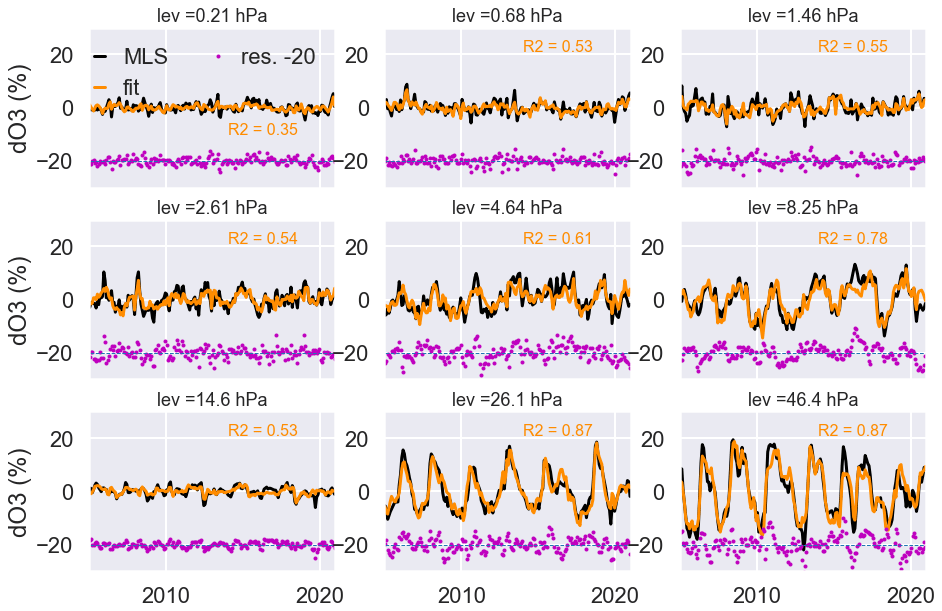
Figure 1Monthly mean ozone anomalies from MLS V5 (black line) for 2005–2020 and corresponding regression fits (orange line) for nine different pressure levels at 1.5∘ N. Goodness of fit (R2) values are also shown with dark-orange-coloured text, and residuals are shown at the bottom of each panel as pink dots. For clarity the residuals are shifted by −20 %.
Different combinations of multivariate regression models are used to estimate long-term ozone trends as well as to quantify the influence of important processes on ozone variability (e.g. Braesicke et al., 2018; SPARC/IO3C/GAW, 2019). Here, we use identical regression models to estimate the SCS in stratospheric ozone from MLS and the model simulations described above. Figure 1 compares MLS ozone anomalies and OLS MLR-fitted regression lines near the Equator (1.5∘ latitude) at nine pressure levels. As expected, the largest ozone variability (≈ ± 15 %) is observed in the lower stratosphere (46.4 hPa) and its magnitude declines almost linearly to higher altitudes except 14.6 hPa. Minimum variability seen near 14.6 hPa is somewhat puzzling, and one possible explanation might be the damping effects of the QBO and semi-annual oscillation-related ozone variability near these levels. Overall, the regression lines show excellent agreement with monthly MLS ozone anomalies (R2 > 0.5) and the residuals are less than a few percent at all levels. Somewhat larger residuals (up to 5 %) occur near 46 hPa (though R2 ≥ 0.85), indicating that even with 24 QBO terms, the regression model has some difficulty in capturing some of the QBO-related ozone variability due to the unusual QBO behaviour over the last decade (e.g. Osprey et al., 2016; Anstey et al., 2021).
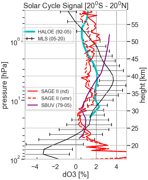
Figure 2Comparison of ozone solar cycle signal (SCS) from various satellite data products for the tropical (20∘ N–20∘ S) region. SCS derived using SAGE II V7.0 (1984–2005) data in terms of number density and mixing ratio units (Dhomse et al., 2016) are shown with solid and dashed red lines, respectively. SCS from HALOE (1992–2005) and SAGE-corrected SBUV (McLinden et al., 2009) (1979–2005) datasets are shown with aqua and purple lines, respectively (Dhomse et al., 2011). SCS from MLS V5 data (2005–2020) is shown with the black line.
Figure 2 shows the MLS observation-based SCS (2005–2020) for the tropical latitude band (20∘ S–20∘ N). The SCS estimated using HALOE (1992–2005, volume mixing ratio, VMR), SAGE II (1984–2005, VMR), SAGE II (1984–2005, number density) and SBUV (1979–2005, VMR) presented in Dhomse et al. (2011, 2015) is also shown for direct comparison. Figure 2 clearly shows that the MLS-based SCS is significantly different to that from all other datasets, although with some similarity to the HALOE-based SCS. A key feature is that the MLS SCS shows a clear broad positive peak in the mid-upper stratosphere that is almost twice as large as any other satellite-data-based SCS reported in the past (e.g. Soukharev and Hood, 2006; Remsberg and Lingenfelser, 2010). On the other hand, our estimates are somewhat consistent with the latest BASIC v2-based estimates (1984–2016) presented in Ball et al. (2019), though MLS shows a ∼ 50 % larger amplitude and it peaks around 40 km against around 35 km in the BASIC data. However, it is important to note that for the 2004–2016 time period, MLS data are used in the BASIC v2 reconstruction. Hence differences between our SCS estimates and that presented in Ball et al. (2019) could be due to using a longer time series (extended time period) or the aliasing effects of other processes (volcanoes, EESC changes).
Near the stratopause region (around 50 km), only MLS and HALOE show a SCS of less than 1 %. The clear difference between MLS versus SAGE II, HALOE and SBUV could be due to a combination of various factors. First, as SAGE and HALOE use the solar occultation technique, even under ideal conditions they provide only about 900 profiles per month over the whole globe. Hence, fewer and sparser profiles are used to calculate monthly mean profiles. In contrast, MLS is a thermal emission limb sounder with a few hundred thousand profiles available for monthly mean calculations. Hence, the MLS-derived SCS suffers minimal impact from non-uniform temporal sampling compared to SAGE and HALOE (e.g. Toohey et al., 2013; Sofieva et al., 2014; Millán et al., 2016). Second, the HALOE and SAGE II data cover a period that has non-linear changes in the equivalent effective stratospheric chlorine loading (EESC, e.g. Newman et al., 2007; Engel et al., 2018a), whereas MLS covers a period where EESC is decreasing almost linearly in response to the actions taken under the Montreal Protocol (e.g. Kohlhepp et al., 2012; Strahan and Douglass, 2018). Third, all of the satellite ozone retrieval algorithms rely on meteorological (re)analysis datasets for the background atmospheric state. Therefore, with technological advances as well as the huge increase in the number of assimilated meteorological observations, the MLS retrieval scheme might have some advantage over the earlier data records. Fourth, the eruption of Mount Pinatubo in June 1991 injected about 14–23 Tg SO2 into the stratosphere (e.g. Guo et al., 2004), leading to significant enhancement in the stratospheric aerosol layer for few years. The enhanced stratospheric aerosol leads to larger ozone retrieval errors for occultation instruments, particularly in the lower stratosphere (e.g. Wang et al., 1996; Thomason, 2012). Enhanced stratospheric aerosol from Mount Pinatubo also caused significant ozone losses and changes in the stratospheric circulation (e.g. Dhomse et al., 2015, 2020) that could have had an impact on the SCS estimates. Fifth, MLS observations cover the recent solar cycle (number 24, 2009–2020), which is one of the weakest cycles (fewer sunspots) over the last century; hence SSI changes may have been somewhat different than for earlier solar cycles. However, a weaker solar cycle does not mean that the SCS during previous cycles would be larger as complications also arise from various complex couplings such as temperature feedback (increased direct radiative heating during solar maxima) and wavelength-dependent photolysis rates (irradiance changes are not uniform across different wavelengths). Sixth, SBUV and SBUV/2 are nadir-viewing instruments with very coarse vertical resolution, especially in the upper stratosphere, which can lead to different (and smoother) SCS profiles.
Another very important difference is observed in the lower stratosphere, where MLS suggests a much smaller (± 1 %) SCS compared to about 5 % SCS in the SAGE II data. It has long been postulated that the lower stratospheric SCS is most probably due to the aliasing effect of volcanic eruptions, QBO and ENSO (e.g. Lee and Smith, 2003; Chiodo et al., 2014). In fact, Dhomse et al. (2011) clearly showed that a CTM simulation with annually repeating dynamics produced a secondary peak in the tropical lower stratosphere that was significantly smaller when simulations are performed with fixed stratospheric aerosol. As there have been no significant volcanic eruptions during the MLS period, this suggests that the large positive SCS in the tropical lower stratosphere reported in SBUV and SAGE II-based studies might be due to non-linear changes in EESC and influences from strongly perturbed stratospheric aerosol layer leading abrupt changes in ozone chemistry and stratospheric dynamics following major volcanic eruptions. Later, we show that a simulation with fixed dynamics does not show a secondary peak for the 2005–2020 time period.

Figure 3Monthly mean ozone anomalies (%) from MLS V5 (black line) and five TOMCAT model simulations for the tropics (20∘ S–20∘ N) for 2005–2020. Ozone anomalies from simulations with NRL V2 (Coddington et al., 2016), SATIRE (Yeo et al., 2014) and SORCE (Harder et al., 2019) are shown with blue, green and red lines, respectively, whereas anomalies from fixed solar fluxes and fixed dynamics (year 2004) are shown with cyan and orange colours. Anomalies are shown for five pressure levels (top to bottom): 1, 3.1, 10, 31 and 100 hPa.
We performed the MLS-like analysis on TOMCAT-simulated ozone profiles from runs A_NRL, B_SAT, C_SOR and D_SFix for all 64 latitude bands and 36 pressure levels ranging from 300 to 0.1 hPa. Comparisons between model (including E_DFix) and MLS tropical (20∘ S–20∘ N) ozone anomalies at five different pressure levels are shown in Fig. 3. Overall, anomalies from the first three simulations (A_NRL, B_SAT and C_SOR) show very similar ozone variations, and mean ozone differences in the tropics are within ± 1 % at all pressure levels. An important aspect in Fig. 3 is that even at 1 hPa modelled ozone differences are always less than 1 %, suggesting consistency between all three solar flux datasets. This clearly highlights that earlier studies showing large negative SCS simulated using SORCE data (e.g. Haigh et al., 2010; Merkel et al., 2011) must have predicted unrealistic ozone variations due to biases in SORCE data as well as much shorter MLS time series.
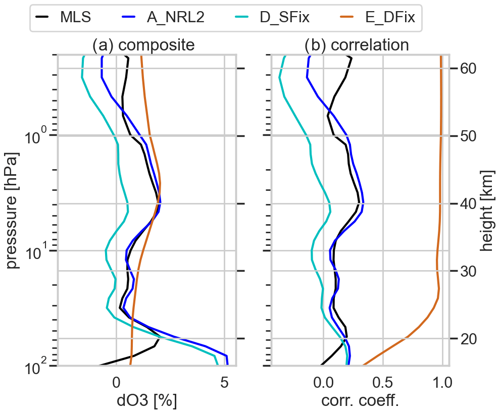
Figure 4(a) MLS ozone profile composite for solar maxima (n=40) and solar minima (n=51) months (black line). Percentage ozone differences for the tropics (20∘ N–20∘ S) between a model simulation with time-varying NRL2 solar flux (A_NRL), fixed solar flux (D_SFix ) and fixed dynamics (E_DFix) simulations are shown with blue, cyan and orange lines, respectively. (b) Correlation coefficient between Mg-ii index and monthly mean ozone anomalies from MLS and simulations A_NRL, D_SFix and E_DFix.
Additionally, anomalies from D_SFix and E_DFix illustrate the effects of solar flux variations. For example, in the lower stratosphere E_DFix shows much smaller variations while D_SFix anomalies are very similar to A_NRL anomalies, confirming exclusive dynamical influence on the ozone variability. However, in the mid-upper stratosphere D_SFix anomalies are clearly smaller than A_NRL, and E_DFix anomalies show variations of about ± 2 %. In order to better understand the effects of time-varying solar fluxes we performed composite and correlation analyses on detrended tropical (20∘ S–20∘ N) ozone anomalies. Figure 4 shows ozone composites for solar maximum and minimum months, as well as the correlation between tropical ozone anomalies and the Mg-ii index. Solar maximum/minimum months are calculated by selecting months when the Mg-ii index is higher/lower than 1 standard deviation. The composite and correlation analyses clearly indicate that A_NRL and MLS-derived estimates are in excellent agreement. As expected, A_NRL shows up to 3 % ozone increase during solar maximum that is almost exclusively because of solar flux variations (E_DFix). An important feature in Fig. 4 is that D_SFix ozone anomalies show very little change between solar maximum and solar minimum months suggesting the implicit SCS in ERA5 dynamics is not enough to simulate observed (MLS-based) ozone variations in the middle and upper stratosphere. As expected run E_DFix anomalies show very high correlation with Mg-ii index throughout the stratosphere. In contrast, both MLS and A_NRL correlation are close to each other with peak values of about 0.3 near 4 hPa and D_SFix anomalies show very little or negligible correlation with the Mg-ii index. Again, this confirms that ERA5 dynamical fields contain only little or no implicit SCS.

Figure 5Latitude–pressure cross sections of solar regression coefficients (or solar cycle signal per 100 solar flux units) for MLS (top row) as well as model simulations A_NRL (second row), B_SAT (third row), C_SOR (fourth row) and D_SFix (bottom row). Regression coefficients are from OLS (first column), lasso (second column), ridge (third column) and elastic net (fourth column) regression models. Stippling indicates regions where regression coefficients are smaller than 1σ uncertainty estimates.
Figure 5 shows SCS estimates for four model simulations as well as MLS data using OLS and three regularised (lasso, ridge, and elastic net) regression models. As expected, regression coefficients from the three regularised models are somewhat smaller than OLS estimates, but overall all the regression models show consistent behaviour. Some key features are a maximum SCS near the tropical and mid-latitude mid-upper stratosphere (near 4 hPa or 40 km) and a negative SCS in the low- and mid-latitude lower stratosphere. It is important to note that the MLS and model-based (A_NRL, B_SAT and C_SOR) SCS are larger than 1σ uncertainty in the tropical and mid-latitude middle stratospheric region (between 30 and 3 hPa). Larger uncertainty in the estimated SCS at the high-latitude lower stratosphere must be due to the relatively short available time series (16 years) and large interannual variability in those regions. Additionally, a second lobe of positive SCS extending from the tropical middle stratosphere to the Arctic lower stratosphere (near 50 hPa) is clearly visible in all the panels. This is consistent with an earlier analysis by Labitzke and Loon (1988).
However, an unexpected feature is that except for the ridge regression model, a large SCS near the Antarctic lower stratosphere is visible in all the models. To our knowledge, this type of strong SCS in the Antarctic stratosphere has not been reported in earlier studies. It could be due to a combination of various factors. First, most of the earlier studies used SBUV, SAGE or HALOE datasets that have limited coverage during dark polar night. Second, the sudden stratospheric warming in the 2019 Antarctic polar vortex stratosphere (e.g. Lim et al., 2020) and wave activity in other recent years, as well as ongoing EESC decreases, might have caused the aliasing effect for the SCS estimation. Actually, close inspection of D_SFix-based estimates suggests that half of the SCS in the Antarctic lower stratosphere may be of dynamical origin.
Another important feature in Fig. 5 is that in the lower stratosphere, all four model simulations (and MLS data) show large negative SCS confirming significant dynamical influence and very little effect from time-varying solar fluxes. However, we find that model-simulated and MLS SCS vary significantly in the mid-latitude lower stratosphere. In the Southern Hemisphere mid-latitudes, MLS data suggest up to −6 % SCS, whereas the model simulations suggest only up −2 %. On the other hand, in the Northern Hemisphere mid-latitudes, MLS data suggest negligible SCS, but model simulations show −4 % SCS. These inter-hemispheric differences between model and MLS data might be due to discrepancies in the ERA5 reanalysis dataset that is used to force TOMCAT (e.g. Chrysanthou et al., 2021).
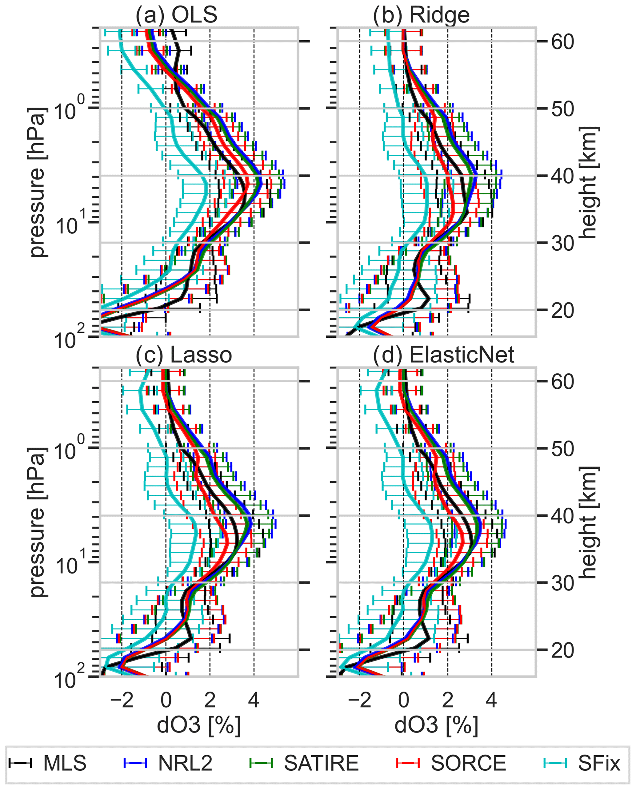
Figure 6Solar cycle signal (SCS) for 2005–2020 period (per 100 solar flux units) in tropical (20∘ N–20∘ S) stratospheric ozone from MLS and ozone profiles from four model simulations (A_NRL, B_SAT, C_SOR and D_SFix) using four types of regression models (a) OLS, (b) lasso, (c) ridge and (d) elastic net. Horizontal lines show averaged 1σ uncertainties.
Figure 6 shows a comparison between the mean SCS for the tropics (20∘ S–20∘ N) from the four different regression models shown in Fig. 4. As seen in Fig. 1, MLS shows the largest SCS near 4 hPa and all the model simulations also show similar SCS profiles. Note that the SCS based on runs A_NRL and B_SAT show nearly identical behaviour. This suggests that although there are non-negligible differences between the construction of the NRL2 and SATIRE solar irradiances (e.g. Yeo et al., 2014; Matthes et al., 2017; Coddington et al., 2019), their wavelength-dependent differences seem to cancel out to produce a nearly identical SCS in stratospheric ozone. In terms of magnitude, OLS-based estimates suggest that MLS shows up to a 3 % SCS near 4 hPa (∼ 40 km), while the NRL2 and SATIRE peaks are about 4.5 % and the SORCE peak lies between the MLS and NRL2 estimates. An important feature in Fig. 5 is that even with regularisation, the MLS-based SCS does not show a significant reduction or alternation, confirming the robustness of the estimated SCS. Most importantly, in Fig. 4 run D_SFix suggested an almost negligible chemical SCS near 4 hPa, but the regression model suggests a SCS of up to 1 % at this altitude demonstrates possibility of some implicit SCS ERA5 dynamical fields.
In the lower stratosphere (below 25 km) all the simulations show a smaller (or more negative) SCS compared to MLS. As expected, the regularisation models (lasso, ridge and elastic net) do not change the profile structure significantly but the estimated magnitudes are somewhat smaller in magnitude with similar behaviour in the three model simulations. Interestingly, even with regularisation the MLS-based SCS does not turn negative in the upper stratosphere, indicating that earlier SORCE-based studies (e.g. Haigh et al., 2010; Merkel et al., 2011; Ball et al., 2016) were likely impaired by their shorter timescales as well as biases in an earlier version of the SORCE dataset.
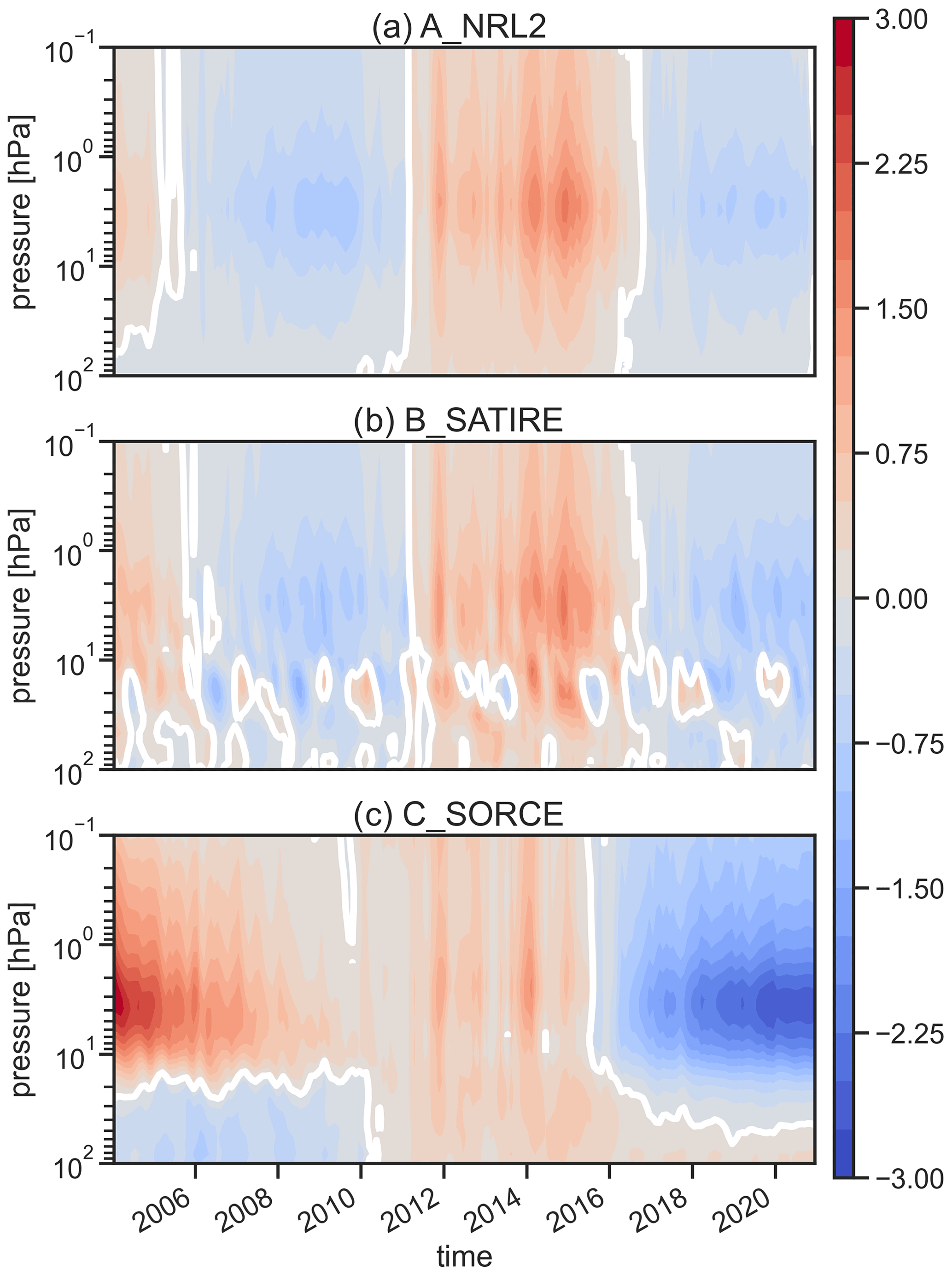
Figure 7Percentage difference in tropical ozone (20∘ N–20∘ S) between a model simulation with time-varying solar flux and a simulation with fixed solar flux for (a) NRL2, (b) SATIRE and (c) SORCE. White-coloured lines show zero contours.
Finally, as run C_SOR also shows good agreement with MLS-based SCS (though within associated uncertainties) similar to runs A_NRL and B_SAT, we analyse the difference between these model simulations. Figure 7 shows tropical (20∘ S–20∘ N) percentage ozone differences between three model simulations with time-varying solar fluxes (A_NRL, B_SAT and C_SOR) and the simulation with fixed solar fluxes (D_SFix, which uses the mean 2005–2020 NRL V2 fluxes). As expected, all comparisons show the largest ozone difference in the mid-upper stratosphere. The time-varying solar flux simulations show a steady decline in ozone differences until 2008 and positive ozone changes after 2011 (solar maximum), followed by an ozone decrease after 2016. Interestingly, run C_SOR show much larger positive differences during 2004/2005 that hardly turn negative in 2008 but show up to −3 % ozone differences in 2016. As seen in Fig. 6, both runs A_NRL and B_SAT show a similar pattern in ozone differences, though the magnitude of ozone change is somewhat larger in run B_SAT. A somewhat different structure in ozone difference during maxima and minima might be due to differences in absolute solar fluxes.
The most interesting aspect in Fig. 7 is that near 5 hPa, run C_SOR shows up to +3 % ozone difference between 2005–2008 compared to about +2 % in runs A_NRL and B_SAT. Similarly, after 2016 run C_SOR shows ozone differences over −3 % in magnitude in the mid-upper stratospheric ozone, which is around 1.5× larger than runs A_NRL and B_SAT. So, although there are significant variations in the ozone difference magnitudes, various model simulations clearly show that all of the solar flux datasets lead to similar patterns in ozone variation (i.e. ozone increases towards solar maxima followed by steady decline towards solar minima). Thus, the results from composite analysis are consistent with the regression analysis. However, the magnitude of ozone variations with respect to the NRL V2-based fixed solar flux simulation is almost double in a simulation with SORCE solar fluxes, whereas regression analysis suggests run C_SOR has a weaker SCS in the low-mid stratosphere. This clearly highlights that model-simulated ozone changes depend on both magnitude of solar irradiances as well as their time variations. Most importantly, somewhat different (and non-linear) ozone differences seen in C_SOR suggest that SORCE solar fluxes may still have some time-varying biases. The larger UV variability reported in earlier versions of the SORCE data (see Sect. 1) is reduced but apparently still larger than that given by SATIRE or NRL v2.
Our key result is that we have presented an analysis of the solar cycle signal (SCS) in stratospheric ozone based on MLS v5 satellite data (2005–2020). Previously, our understanding of the ozone SCS has been largely based on 22 years of SAGE II v7 data (Dhomse et al., 2016; Maycock et al., 2016). As the MLS satellite instrument has a much better spatial coverage than any other ozone dataset providing more than 16 years of continuous ozone profile measurements, it is ideally suited for re-evaluating our understanding of the processes controlling/modifying stratospheric ozone. MLS data also cover a period where EESC changes are almost linear and there has been no major volcanically induced perturbation to the stratospheric aerosol layer. Hence the SCS attribution is relatively cleaner than in previous datasets where trends as well as attribution are complicated as they include periods with strong volcanic eruptions.
Our analysis suggests a single-peak-structured SCS in the tropical stratosphere, which is significantly different to that derived in previous studies based on SAGE II and SBUV datasets during earlier periods. In contrast, the MLS-based SCS shows a similar structure to that from HALOE data, although its peak amplitude near 3 hPa is almost double that of HALOE (up to 3 %). The lack of a secondary peak in MLS satellite data suggests that the Mount Pinatubo-volcanic-eruption-induced chemical and dynamical changes might have caused an aliasing effect in the estimated SCS presented in earlier studies. However, this analysis is consistent with the postulations discussed in modelling studies such as Lee and Smith (2003), Dhomse et al. (2011), and Chiodo et al. (2014).
We also performed three model sensitivity simulations with different solar flux datasets: NRL2, SATIRE and SORCE. We find that the SCS from the simulation with SORCE fluxes is somewhat smaller in magnitude but is within the uncertainties seen in the MLS-derived SCS as well as NRL2 and SATIRE data. Overall, all three model simulations show SCS structures very similar to that in MLS data. Importantly, it suggests that with recent adjustments and corrections (Harder et al., 2019), SORCE data can be used to study the effects of solar flux variations, though some time-varying biases in SORCE data cannot be ruled out. We also performed an ensemble of linear regression models (OLS, lasso, ridge and elastic net) that confirm the robustness of the SCS. All of the regression models show a broad peak near low-mid latitudes around 4 hPa. MLS data and model simulations also indicate a much larger SCS in the Antarctic stratosphere that could be due to the aliasing effect of ozone recovery due to a decrease in EESC loading as well as changes in stratospheric transport in the Southern Hemisphere. Finally, regression and composite analyses of model simulations with respect to fixed solar flux simulations suggest that both absolute magnitude as well as time variations in solar flux forcing datasets play key roles in SCS estimates.
MLS data are available at https://disc.gsfc.nasa.gov/datasets?keywords=ML2O3_005&page=1 (NASA Earth Data, 2022) following download instructions from https://disc.gsfc.nasa.gov/data-access (last access: January 2022). TOMCAT data can be downloaded from https://doi.org/10.5281/zenodo.5875190 (Dhomse et al., 2022).
The NRL V2 dataset is available via the LaTiS web service interface at https://lasp.colorado.edu/lisird/latis/dap/nrl2_ssi_P1M (University of Colorado, 2021a). SORCE data are available at https://lasp.colorado.edu/data/sorce/ssi_data/composite/sorce_L3_combined_c24h_20030225_20200225.nc (University of Colorado, 2021b). Combined SATIRE (SATIRE-T and SATIRE-S) datasets are available at https://doi.org/10.17617/1.5U (Max Planck Institute for Solar System Research, 2021).
The solar activity proxy index (Mg II index) is available at http://www.iup.uni-bremen.de/UVSAT/Datasets/mgii (Universität Bremen, 2021). QBO, ENSO, AO and AAO indices are obtained from the Climate Prediction Center, via https://www.cpc.ncep.noaa.gov/ (NOAA, 2021).
The supplement related to this article is available online at: https://doi.org/10.5194/acp-22-903-2022-supplement.
SSD designed the research, analysed the data, and prepared the figures. MPC, SSD, WF and RH designed the TOMCAT model simulations which were performed by MPC. GWM, MLS and MW provided insightful comments about stratospheric aerosol, MLS satellite data and the Mg-II solar index. SSD and MPC wrote the article, with contributions from all co-authors.
The contact author has declared that neither they nor their co-authors have any competing interests.
Publisher's note: Copernicus Publications remains neutral with regard to jurisdictional claims in published maps and institutional affiliations.
We are grateful to William Ball for useful comments. We thank the European Centre for Medium-Range Weather Forecasts for providing their analyses. The model simulations were performed on the UK national Archer and Leeds Arc4 HPC systems.
This research has been supported by the Natural Environment Research Council (grant no. NE/R001782/1) and the National Centre for Earth Observation (grant no. NE/R016518/1). Work at the Jet Propulsion Laboratory, California Institute of Technology, was carried out under a contract with the National Aeronautics and Space Administration.
This paper was edited by Jens-Uwe Grooß and reviewed by two anonymous referees.
Anstey, J. A., Banyard, T. P., Butchart, N., Coy, L., Newman, P. A., Osprey, S., and Wright, C. J.: Prospect of Increased Disruption to the QBO in a Changing Climate, Geophys. Res. Lett., 48, e2021GL093058, https://doi.org/10.1029/2021GL093058, 2021. a
Ball, W., Haigh, J., Rozanov, E., Kuchar, A., Sukhodolov, T., Tummon, F., Shapiro, A., and Schmutz, W.: High solar cycle spectral variations inconsistent with stratospheric ozone observations, Nat. Geosci., 9, 206–209, 2016. a
Ball, W. T., Rozanov, E. V., Alsing, J., Marsh, D. R., Tummon, F., Mortlock, D. J., Kinnison, D., and Haigh, J. D.: The Upper Stratospheric Solar Cycle Ozone Response, Geophys. Res. Lett., 46, 1831–1841, https://doi.org/10.1029/2018GL081501, 2019. a, b, c
Braesicke, P., Neu, J. L., Fioletov, V. E., Godin-Beekmann, S., Hubert, D., Petropavlovskikh, I., Shiotani, M., Sinnhuber, B.-M., Ball, W., Chang, K.-L., Damadeo, R., Dhomse, S., Frith, S., Gaudel, A., Hassler, B., Hossaini, R., Kremser, S., Misios, S., Morgenstern, O., Salawitch, R. J., Sofieva, V., Tourpali, K., Tweedy, O., and Zawada, D.: Update on Global Ozone: Past, Present, and Future, Chapter 3, in: WMO Scientific Assessment of Ozone Depletion (2018), WMO (World Meteorological Organization), Geneva, Switzerland, available at: https://elib.dlr.de/135132/ (last access: June 2021), 2018. a
Brasseur, G.: The response of the middle atmosphere to long-term and short-term solar variability: a two-dimensional model, J. Geophys. Res., 98, 23079–23090, https://doi.org/10.1029/93JD02406, 1993. a
Chandra, S.: An assessment of possible ozone-solar cycle relationship inferred from NIMBUS 4 BUV data, J. Geophys. Res.-Atmos., 89, 1373–1379, https://doi.org/10.1029/JD089iD01p01373, 1984. a
Chandra, S. and McPeters, R. D.: The solar cycle variation of ozone in the stratosphere inferred from Nimbus 7 and NOAA 11 satellites, J. Geophys. Res., 99, 20665–20671, https://doi.org/10.1029/94jd02010, 1994. a
Chandra, S., Froidevaux, L., Waters, J. W., White, O. R., Rottman, G. J., Prinz, D. K., and Brueckner, G. E.: Ozone variability in the upper stratosphere during the declining phase of the solar cycle 22, Geophys. Res. Lett., 23, 2935–2938, https://doi.org/10.1029/96GL02760, 1996. a
Chapman, S. C., McIntosh, S. W., Leamon, R. J., and Watkins, N. W.: Quantifying the Solar Cycle Modulation of Extreme Space Weather, Geophys. Res. Lett., 47, e2020GL087795, https://doi.org/10.1029/2020GL087795, 2020. a
Chiodo, G., Marsh, D. R., Garcia-Herrera, R., Calvo, N., and García, J. A.: On the detection of the solar signal in the tropical stratosphere, Atmos. Chem. Phys., 14, 5251–5269, https://doi.org/10.5194/acp-14-5251-2014, 2014. a, b, c
Chipperfield, M. P.: New version of the TOMCAT/SLIMCAT off-line chemical transport model: Intercomparison of stratospheric tracer experiments, Q. J. Roy. Meteor. Soc., 132, 1179–1203, https://doi.org/10.1256/qj.05.51, 2006. a
Chipperfield, M. P., Bekki, S., Dhomse, S., Harris, N. R., Hassler, B., Hossaini, R., Steinbrecht, W., Thiéblemont, R., and Weber, M.: Detecting recovery of the stratospheric ozone layer, Nature, 549, 211–218, 2017. a
Chrysanthou, A., Dhomse, S., Feng, W., Yajun, L., Hossaini, R., Ball, W., and Chipperfield, M.: The conundrum of the recent variations in the lower stratospheric ozone: An update, Quadrennial Ozone Symposium, Symposium, Online Meeting (live-streamed from Daejeon, S. Korea), available at: http://qos2021.yonsei.ac.kr/overview.php, last access: 1 December 2021. a
Coddington, O., Lean, J. L., Pilewskie, P., Snow, M., and Lindholm, D.: A Solar Irradiance Climate Data Record, B. Am. Meteorol. Soc., 97, 1265–1282, https://doi.org/10.1175/BAMS-D-14-00265.1, 2016. a, b, c
Coddington, O., Lean, J., Pilewskie, P., Snow, M., Richard, E., Kopp, G., Lindholm, C., DeLand, M., Marchenko, S., Haberreiter, M., and Baranyi, T.: Solar Irradiance Variability: Comparisons of Models and Measurements, Earth Space Sci., 6, 2525–2555, https://doi.org/10.1029/2019EA000693, 2019. a, b
Dhomse, S., Weber, M., Wohltmann, I., Rex, M., and Burrows, J. P.: On the possible causes of recent increases in northern hemispheric total ozone from a statistical analysis of satellite data from 1979 to 2003, Atmos. Chem. Phys., 6, 1165–1180, https://doi.org/10.5194/acp-6-1165-2006, 2006. a
Dhomse, S., Chipperfield, M. P., Feng, W., and Haigh, J. D.: Solar response in tropical stratospheric ozone: a 3-D chemical transport model study using ERA reanalyses, Atmos. Chem. Phys., 11, 12773–12786, https://doi.org/10.5194/acp-11-12773-2011, 2011. a, b, c, d, e, f, g, h
Dhomse, S., Chipperfield, M., Damadeo, R., Zawodny, J., Ball, W., Feng, W., Hossaini, R., Mann, G., and Haigh, J.: On the ambiguous nature of the 11 year solar cycle signal in upper stratospheric ozone, Geophys. Res. Lett., 43, 7241–7249, https://doi.org/10.1002/2016GL069958, 2016. a, b, c
Dhomse, S., Feng, W., Montzka, S. A., Hossaini, R., Keeble, J., Pyle, J., Daniel, J., and Chipperfield, M.: Delay in recovery of the Antarctic ozone hole from unexpected CFC-11 emissions, Nat. Commun., 10, 1–12, 2019. a
Dhomse, S. S., Chipperfield, M. P., Feng, W., Ball, W. T., Unruh, Y. C., Haigh, J. D., Krivova, N. A., Solanki, S. K., and Smith, A. K.: Stratospheric O3 changes during 2001–2010: the small role of solar flux variations in a chemical transport model, Atmos. Chem. Phys., 13, 10113–10123, https://doi.org/10.5194/acp-13-10113-2013, 2013. a, b
Dhomse, S. S., Chipperfield, M. P., Feng, W., Hossaini, R., Mann, G. W., and Santee, M. L.: Revisiting the hemispheric asymmetry in midlatitude ozone changes following the Mount Pinatubo eruption: A 3-D model study, Geophys. Res. Lett., 42, 3038–3047, https://doi.org/10.1002/2015GL063052, 2015. a, b, c, d, e, f
Dhomse, S. S., Mann, G. W., Antuña Marrero, J. C., Shallcross, S. E., Chipperfield, M. P., Carslaw, K. S., Marshall, L., Abraham, N. L., and Johnson, C. E.: Evaluating the simulated radiative forcings, aerosol properties, and stratospheric warmings from the 1963 Mt Agung, 1982 El Chichón, and 1991 Mt Pinatubo volcanic aerosol clouds, Atmos. Chem. Phys., 20, 13627–13654, https://doi.org/10.5194/acp-20-13627-2020, 2020. a, b
Dhomse, S. S., Chipperfield, M. P., Wuhu, F., and Hossaini, R. H.: TOMCAT CTM simulated ozone profiles using NRL2, SATIRE and SORCE solar fluxes, Zenodo [data set], https://doi.org/10.5281/zenodo.5875190, 2022. a
Engel, A., Bönisch, H., Ostermöller, J., Chipperfield, M. P., Dhomse, S., and Jöckel, P.: A refined method for calculating equivalent effective stratospheric chlorine, Atmos. Chem. Phys., 18, 601–619, https://doi.org/10.5194/acp-18-601-2018, 2018a. a
Engel, A., Rigby, M., Burkholder, J., Fernandez, R., Froidevaux, L., Hall, B., Hossaini, R., Saito, T., Vollmer, M., and Yao, B.: Update on Ozone-Depleting Substances (ODSs) and other gases of interest to the Montreal Protocol, Chapter 1, in: Scientific Assessment of Ozone Depletion: 2018, Global Ozone Research and Monitoring Project, Tech. rep., WMO (World Meteorological Organization), Geneva, Switzerland, 2018b. a
Ermolli, I., Matthes, K., Dudok de Wit, T., Krivova, N. A., Tourpali, K., Weber, M., Unruh, Y. C., Gray, L., Langematz, U., Pilewskie, P., Rozanov, E., Schmutz, W., Shapiro, A., Solanki, S. K., and Woods, T. N.: Recent variability of the solar spectral irradiance and its impact on climate modelling, Atmos. Chem. Phys., 13, 3945–3977, https://doi.org/10.5194/acp-13-3945-2013, 2013. a, b
Feng, W., Chipperfield, M. P., Dorf, M., Pfeilsticker, K., and Ricaud, P.: Mid-latitude ozone changes: studies with a 3-D CTM forced by ERA-40 analyses, Atmos. Chem. Phys., 7, 2357–2369, https://doi.org/10.5194/acp-7-2357-2007, 2007. a
Feng, W., Dhomse, S. S., Arosio, C., Weber, M., Burrows, J. P., Santee, M. L., and Chipperfield, M. P.: Arctic Ozone Depletion in 2019/20: Roles of Chemistry, Dynamics and the Montreal Protocol, Geophys. Res. Lett., 48, e2020GL091911, https://doi.org/10.1029/2020GL091911, 2021. a
Fleming, E. L., Chandra, S., Jackman, C. H., Considine, D. B., and Douglass, A. R.: The middle atmospheric response to short and long term solar UV variations: analysis of observations and 2D model results, J. Atmos. Terr. Phys., 57, 333–365, https://doi.org/10.1016/0021-9169(94)E0013-D, 1995. a, b
Garcia, R. R., Solomon, S., Roble, R. G., and Rusch, D. W.: A numerical response of the middle atmosphere to the 11-year solar cycle, Planet. Space Sci., 32, 411–423, https://doi.org/10.1016/0032-0633(84)90121-1, 1984. a
Gray, L. J., Beer, J., Geller, M., Haigh, J. D., Lockwood, M., Matthes, K., Cubasch, U., Fleitmann, D., Harrison, G., Hood, L., Luterbacher, J., Meehl, G. A., Shindell, D., van Geel, B., and White, W.: Solar influences on climate, Rev. Geophys., 48, RG4001, https://doi.org/10.1029/2009RG000282, 2010. a
Guo, S., Bluth, G. J. S., Rose, W. I., Watson, I. M., and Prata, A. J.: Reevaluation of SO2 release of the 15 June 1991 Pinatubo eruption using ultraviolet and infrared satellite sensors, Geochem. Geophy. Geosy., 5, Q04001, https://doi.org/10.1029/2003GC000654, 2004. a
Haberreiter, M., Schöll, M., Dudok de Wit, T., Kretzschmar, M., Misios, S., Tourpali, K., and Schmutz, W.: A new observational solar irradiance composite, J. Geophys. Res.-Space, 122, 5910–5930, 2017. a
Haigh, J., Winning, A., Toumi, R., and Harder, J.: An influence of solar spectral variations on radiative forcing of climate, Nature, 467, 696–699, https://doi.org/10.1038/nature09426, 2010. a, b, c
Haigh, J. D.: The role of stratospheric ozone in modulating the solar radiative forcing of climate, Nature, 370, 544–546, 1994. a
Harder, J. W., Fontenla, J. M., Pilewskie, P., Richard, E. C., and Woods, T. N.: Trends in solar spectral irradiance variability in the visible and infrared, Geophys. Res. Lett., 36, L07801, https://doi.org/10.1029/2008GL036797, 2009. a
Harder, J. W., Beland, S., and Snow, M.: SORCE-based solar spectral irradiance (SSI) record for input into chemistry-climate studies, Earth Space Sci., 6, 2487–2507, 2019. a, b, c
Hersbach, H., Bell, B., Berrisford, P., Hirahara, S., Horányi, A., Muñoz-Sabater, J., Nicolas, J., Peubey, C., Radu, R., Schepers, D., Simmons, A., Soci, C., Abdalla, S., Abellan, X., Balsamo, G., Bechtold, P., Biavati, G., Bidlot, J., Bonavita, M., De Chiara, G., Dahlgren, P., Dee, D., Diamantakis, M., Dragani, R., Flemming, J., Forbes, R., Fuentes, M., Geer, A., Haimberger, L., Healy, S., Hogan, R. J., Hólm, E., Janisková, M., Keeley, S., Laloyaux, P., Lopez, P., Lupu, C., Radnoti, G., de Rosnay, P., Rozum, I., Vamborg, F., Villaume, S., and Thépaut, J.-N.: The ERA5 global reanalysis, Q. J. Roy. Meteor. Soc., 146, 1999–2049, https://doi.org/10.1002/qj.3803, 2020. a
Hoerl, A. E. and Kennard, R. W.: Ridge regression: Biased estimation for nonorthogonal problems, Technometrics, 12, 55–67, 1970. a
Holton, J. R. and Tan, H.-C.: The quasi-biennial oscillation in the Northern Hemisphere lower stratosphere, J. Meteorol. Soc. Jpn. Ser. II, 60, 140–148, 1982. a
Hood, L. L., Jirikowic, J. L., and McCormack, J. P.: Quasi-Decadal Variability of the Stratosphere: Influence of Long-Term Solar Ultraviolet Variations, J. Atmos. Sci., 50, 24, 3941–3958, https://doi.org/10.1175/1520-0469, 1993. a
Hossaini, R., Chipperfield, M. P., Montzka, S. A., Leeson, A. A., Dhomse, S. S., and Pyle, J. A.: The increasing threat to stratospheric ozone from dichloromethane, Nat. Commun., 8, 1–9, 2017. a
Hossaini, R., Atlas, E., Dhomse, S. S., Chipperfield, M. P., Bernath, P. F., Fernando, A. M., Mühle, J., Leeson, A. A., Montzka, S. A., Feng, W., Harrison, J. J., Krummel, P., Vollmer, M. K., Reimann, S., O'Doherty, S., Young, D., Maione, M., Arduini, J., and Lunder, C. R.: Recent trends in stratospheric chlorine from very short-lived substances, J. Geophys. Res.-Atmos., 124, 2318–2335, 2019. a
Huang, T. Y. and Brasseur, G. P.: Effect of long-term solar variability in a two-dimensional interactive model of the middle atmosphere, J. Geophys. Res., 98, 20413–20427, https://doi.org/10.1029/93jd02187, 1993. a
Kohlhepp, R., Ruhnke, R., Chipperfield, M. P., De Mazière, M., Notholt, J., Barthlott, S., Batchelor, R. L., Blatherwick, R. D., Blumenstock, Th., Coffey, M. T., Demoulin, P., Fast, H., Feng, W., Goldman, A., Griffith, D. W. T., Hamann, K., Hannigan, J. W., Hase, F., Jones, N. B., Kagawa, A., Kaiser, I., Kasai, Y., Kirner, O., Kouker, W., Lindenmaier, R., Mahieu, E., Mittermeier, R. L., Monge-Sanz, B., Morino, I., Murata, I., Nakajima, H., Palm, M., Paton-Walsh, C., Raffalski, U., Reddmann, Th., Rettinger, M., Rinsland, C. P., Rozanov, E., Schneider, M., Senten, C., Servais, C., Sinnhuber, B.-M., Smale, D., Strong, K., Sussmann, R., Taylor, J. R., Vanhaelewyn, G., Warneke, T., Whaley, C., Wiehle, M., and Wood, S. W.: Observed and simulated time evolution of HCl, ClONO2, and HF total column abundances, Atmos. Chem. Phys., 12, 3527–3556, https://doi.org/10.5194/acp-12-3527-2012, 2012. a
Krivova, N. A., Vieira, L. E. A., and Solanki, S. K.: Reconstruction of solar spectral irradiance since the Maunder minimum, J. Geophys. Res.-Space, 115, A12112, https://doi.org/10.1029/2010JA015431, 2010. a
Labitzke, K. and Loon, H. V.: Associations between the 11-year solar cycle, the QBO and the atmosphere. Part I: the troposphere and stratosphere in the northern hemisphere in winter, J. Atmos. Terr. Phys., 50, 197–206, https://doi.org/10.1016/0021-9169(88)90068-2, 1988. a
Lean, J.: Evolution of the Sun's spectral irradiance since the Maunder Minimum, Geophys. Res. Lett., 27, 2425–2428, 2000. a
Lean, J. L. and DeLand, M. T.: How Does the Sun's Spectrum Vary?, J. Climate, 25, 2555–2560, https://doi.org/10.1175/JCLI-D-11-00571.1, 2012. a
Lee, H. and Smith, A.: Simulation of the combined effects of solar cycle, quasi-biennial oscillation, and volcanic forcing on stratospheric ozone changes in recent decades, J. Geophys. Res.-Atmos., 108, 4049, https://doi.org/10.1029/2001JD001503, 2003. a, b, c
Lim, E.-P., Hendon, H. H., Butler, A. H., Garreaud, R. D., Polichtchouk, I., Shepherd, T. G., Scaife, A., Comer, R., Coy, L., Newman, P. A., Thompon, D. W. J., and Nakamura, H.: The 2019 Antarctic sudden stratospheric warming, SPARC Newsletter, 54, 10–13, 2020. a
Livesey, N. J., Read, W. G., Wagner, P. A., Froidevaux, L., Santee, M. L., Schwartz, M. J., Lambert, A., Millan, L., Pumphrey, H. C., Manney, G. L., A., F. R., Jarnot, R. F., Knosp, B. W., and Lay, R. R.: EOS MLS Version 5.0x Level 2 and 3 data quality and description document, Tech. Rep. No. JPL D-105336 Rev. A, Jet Propulsion Laboratory, California Institute of Technology, Pasadena, CA, 2020. a
Matthes, K., Funke, B., Andersson, M. E., Barnard, L., Beer, J., Charbonneau, P., Clilverd, M. A., Dudok de Wit, T., Haberreiter, M., Hendry, A., Jackman, C. H., Kretzschmar, M., Kruschke, T., Kunze, M., Langematz, U., Marsh, D. R., Maycock, A. C., Misios, S., Rodger, C. J., Scaife, A. A., Seppälä, A., Shangguan, M., Sinnhuber, M., Tourpali, K., Usoskin, I., van de Kamp, M., Verronen, P. T., and Versick, S.: Solar forcing for CMIP6 (v3.2), Geosci. Model Dev., 10, 2247–2302, https://doi.org/10.5194/gmd-10-2247-2017, 2017. a
Maycock, A. C., Matthes, K., Tegtmeier, S., Thiéblemont, R., and Hood, L.: The representation of solar cycle signals in stratospheric ozone – Part 1: A comparison of recently updated satellite observations, Atmos. Chem. Phys., 16, 10021–10043, https://doi.org/10.5194/acp-16-10021-2016, 2016. a, b
McCormack, J. P. and Hood, L. L.: Apparent solar cycle variations of upper stratospheric ozone and temperature: Latitude and seasonal dependences, J. Geophys. Res.-Atmos., 101, 20933–20944, https://doi.org/10.1029/96jd01817, 1996. a
McLinden, C. A., Tegtmeier, S., and Fioletov, V.: Technical Note: A SAGE-corrected SBUV zonal-mean ozone data set, Atmos. Chem. Phys., 9, 7963–7972, https://doi.org/10.5194/acp-9-7963-2009, 2009. a
Merkel, A. W., Harder, J. W., Marsh, D. R., Smith, A. K., Fontenla, J. M., and Woods, T. N.: The impact of solar spectral irradiance variability on middle atmospheric ozone, Geophys. Res. Lett., 38, L13802, https://doi.org/10.1029/2011GL047561, 2011. a, b, c
Millán, L. F., Livesey, N. J., Santee, M. L., Neu, J. L., Manney, G. L., and Fuller, R. A.: Case studies of the impact of orbital sampling on stratospheric trend detection and derivation of tropical vertical velocities: solar occultation vs. limb emission sounding, Atmos. Chem. Phys., 16, 11521–11534, https://doi.org/10.5194/acp-16-11521-2016, 2016. a
Max Planck Institute for Solar System Research (MPS): THE SUN AND THE EARTH'S CLIMATE, available at: https://doi.org/10.17617/1.5U, last access: June 2021. a
NASA Earth Data: MLS data, NASA [data set], available at https://disc.gsfc.nasa.gov/datasets?keywords=ML2O3_005&page=1, last access: January 2022. a
Newchurch, M., Yang, E.-S., Cunnold, D., Reinsel, G. C., Zawodny, J., and Russell III, J. M.: Evidence for slowdown in stratospheric ozone loss: First stage of ozone recovery, J. Geophys. Res.-Atmos., 108, 4507, https://doi.org/10.1029/2003JD003471, 2003. a
Newman, P. A., Daniel, J. S., Waugh, D. W., and Nash, E. R.: A new formulation of equivalent effective stratospheric chlorine (EESC), Atmos. Chem. Phys., 7, 4537–4552, https://doi.org/10.5194/acp-7-4537-2007, 2007. a
NOAA: Climate News, available at: https://www.cpc.ncep.noaa.gov/, last access: June 2021. a
Osprey, S. M., Butchart, N., Knight, J. R., Scaife, A. A., Hamilton, K., Anstey, J. A., Schenzinger, V., and Zhang, C.: An unexpected disruption of the atmospheric quasi-biennial oscillation, Science, 353, 1424–1427, https://doi.org/10.1126/science.aah4156, 2016. a
Pedregosa, F., Varoquaux, G., Gramfort, A., Michel, V., Thirion, B., Grisel, O., Blondel, M., Prettenhofer, P., Weiss, R., Dubourg, V., Vanderplas, J., Passos, A., Cournapeau, D., Brucher, M., Perrot, M., and Duchesnay, É.: Scikit-learn: Machine Learning in Python, J. Mach. Learn. Res., 12, 2825–2830, 2011. a
Remsberg, E.: On the response of Halogen Occultation Experiment (HALOE) stratospheric ozone and temperature to the 11-year solar cycle forcing, J. Geophys. Res.-Atmos., 113, D22304, https://doi.org/10.1029/2008JD010189, 2008. a
Remsberg, E. and Lingenfelser, G.: Analysis of SAGE II ozone of the middle and upper stratosphere for its response to a decadal-scale forcing, Atmos. Chem. Phys., 10, 11779–11790, https://doi.org/10.5194/acp-10-11779-2010, 2010. a, b, c
SILSO World Data Center: Sunspot Number and Long-term Solar Observations, Royal Observatory of Belgium, Monthly Report on the International Sunspot Number, on-line Sunspot Number catalogue available at: https://wwwbis.sidc.be/silso/datafiles (last access: June 2021), 2005–2020, 2021. a
Smith, A. and Matthes, K.: Decadal-scale periodicities in the stratosphere associated with the solar cycle and the QBO, J. Geophys. Res., 113, D05311, https://doi.org/10.1029/2007JD009051, 2008. a
Snow, M., Weber, M., Machol, J., Viereck, R., and Richard, E.: Comparison of Magnesium II core-to-wing ratio observations during solar minimum 23/24, J. Space Weather Space, 4, A04, https://doi.org/10.1051/swsc/2014001, 2014. a
Sofieva, V. F., Kalakoski, N., Päivärinta, S.-M., Tamminen, J., Laine, M., and Froidevaux, L.: On sampling uncertainty of satellite ozone profile measurements, Atmos. Meas. Tech., 7, 1891–1900, https://doi.org/10.5194/amt-7-1891-2014, 2014. a
Soukharev, B. E. and Hood, L. L.: Solar cycle variation of stratospheric ozone: Multiple regression analysis of long-term satellite data sets and comparisons with models, J. Geophys. Res.-Atmos., 111, D20314, https://doi.org/10.1029/2006JD007107, 2006. a, b
SPARC: SPARC CCMVal Report on the Evaluation of Chemistry-Climate Models, Tech. rep., SPARC, available at: http://www.sparc-climate.org/publications/sparc-reports/ (last access: June 2021), 2010. a, b
SPARC/IO3C/GAW: SPARC/IO3C/GAW Report on Long-term Ozone Trends and Uncertainties in the Stratosphere, edited by: Petropavlovskikh, I., Godin-Beekmann, S., Hubert, D., Damadeo, R., Hassler, B., and Sofieva, V., SPARC Report No. 9, GAW Report No. 241, WCRP-17/2018, https://doi.org/10.17874/f899e57a20b, electronic version available at: http://www.sparc-climate.org/publications/sparc-reports/sparc-report-no9 (last access : June 2021), 2019. a
Steinbrecht, W., Claude, H., and Winkler, P.: Enhanced upper stratospheric ozone: Sign of recovery or solar cycle effect?, J. Geophys. Res., 109, D02308, https://doi.org/10.1029/2003JD004284, 2004. a
Strahan, S. E. and Douglass, A. R.: Decline in Antarctic ozone depletion and lower stratospheric chlorine determined from Aura Microwave Limb Sounder observations, Geophys. Res. Lett., 45, 382–390, 2018. a
Swartz, W. H., Stolarski, R. S., Oman, L. D., Fleming, E. L., and Jackman, C. H.: Middle atmosphere response to different descriptions of the 11-yr solar cycle in spectral irradiance in a chemistry-climate model, Atmos. Chem. Phys., 12, 5937–5948, https://doi.org/10.5194/acp-12-5937-2012, 2012. a
Thomason, L. W.: Toward a combined SAGE II-HALOE aerosol climatology: an evaluation of HALOE version 19 stratospheric aerosol extinction coefficient observations, Atmos. Chem. Phys., 12, 8177–8188, https://doi.org/10.5194/acp-12-8177-2012, 2012. a
Tibshirani, R.: Regression shrinkage and selection via the lasso, J. Roy. Stat. Soc. B Met., 58, 267–288, 1996. a
Toohey, M., Hegglin, M. I., Tegtmeier, S., Anderson, J., Añel, J. A., Bourassa, A., Brohede, S., Degenstein, D., Froidevaux, L., Fuller, R., Funke, B., Gille, J., Jones, A., Kasai, Y., Krüger, K., Kyrölä, E., Neu, J. L., Rozanov, A., Smith, L., Urban, J., von Clarmann, T., Walker, K. A., and Wang, R. H. J.: Characterizing sampling biases in the trace gas climatologies of the SPARC Data Initiative, J. Geophys. Res.-Atmos., 118, 11847–11862, https://doi.org/10.1002/jgrd.50874, 2013. a
Universität Bremen: Observations of solar activity by GOME, SCIAMACHY, and GOME-2, Universität Bremen [data set], available at: http://www.iup.uni-bremen.de/UVSAT/Datasets/mgii, last access: June 2021. a
University of Colorado: nrl2_ssi_P1M data, University of Colorado [data set], available at: https://lasp.colorado.edu/lisird/latis/dap/nrl2_ssi_P1M, last access: June 2021a. a
University of Colorado: sorce_L3_combined_c24h_20030225_ 20200225 data, University of Colorado [data set], available at: https://lasp.colorado.edu/data/sorce/ssi_data/composite/sorce_L3_combined_c24h_20030225_20200225.nc, last access: June 2021b. a
Wang, H., Cunnold, D., and Bao, X.: A critical analysis of stratospheric aerosol and gas experiment ozone trends, J. Geophys. Res.-Atmos., 101, 12495–12514, 1996. a, b, c
Weber, M., Arosio, C., Feng, W., Dhomse, S. S., Chipperfield, M. P., Meier, A., Burrows, J. P., Eichmann, K.-U., Richter, A., and Rozanov, A.: The Unusual Stratospheric Arctic Winter 2019/20: Chemical Ozone Loss From Satellite Observations and TOMCAT Chemical Transport Model, J. Geophys. Res.-Atmos., 126, e2020JD034386, https://doi.org/10.1029/2020JD034386, 2021. a
Yeo, K., Krivova, N., Solanki, S., and Glassmeier, K.: Reconstruction of total and spectral solar irradiance from 1974 to 2013 based on KPVT, SoHO/MDI, and SDO/HMI observations, Astron. Astrophys., 570, A85, https://doi.org/10.1051/0004-6361/201423628, 2014. a, b, c, d
Zou, H. and Hastie, T.: Regularization and variable selection via the elastic net, J. Roy. Stat. Soc. B Met., 67, 301–320, 2005. a