the Creative Commons Attribution 4.0 License.
the Creative Commons Attribution 4.0 License.
 | 19 Jan 2022
On the cross-tropopause transport of water by tropical convective overshoots: a mesoscale modelling study constrained by in situ observations during the TRO-Pico field campaign in Brazil
Abhinna K. Behera
Emmanuel D. Rivière
Sergey M. Khaykin
Virginie Marécal
Mélanie Ghysels
Jérémie Burgalat
Gerhard Held
Deep convection overshooting the lowermost stratosphere is well known for its role in the local stratospheric water vapour (WV) budget. While it is seldom the case, local enhancement of WV associated with stratospheric overshoots is often published. Nevertheless, one debatable topic persists regarding the global impact of this event with respect to the temperature-driven dehydration of air parcels entering the stratosphere. As a first step, it is critical to quantify their role at a cloud-resolving scale before assessing their impact on a large scale in a climate model. It would lead to a nudging scheme for large-scale simulation of overshoots.
This paper reports on the local enhancements of WV linked to stratospheric overshoots, observed during the TRO-Pico campaign conducted in March 2012 in Bauru, Brazil, using the BRAMS (Brazilian version of the Regional Atmospheric Modeling System; RAMS) mesoscale model. Since numerical simulations depend on the choice of several preferred parameters, each having its uncertainties, we vary the microphysics or the vertical resolution while simulating the overshoots. Thus, we produce a set of simulations illustrating the possible variations in representing the stratospheric overshoots. To better resolve the stratospheric hydration, we opt for simulations with the 800 m horizontal-grid-point presentation. Next, we validate these simulations against the Bauru S-band radar echo tops and the TRO-Pico balloon-borne observations of WV and particles. Two of the three simulations' setups yield results compatible with the TRO-Pico observations. From these two simulations, we determine approximately 333–2000 t of WV mass prevailing in the stratosphere due to an overshooting plume depending on the simulation setup. About 70 % of the ice mass remains between the 380 and 385 K isentropic levels. The overshooting top comprises pristine ice and snow, while aggregates only play a role just above the tropopause. Interestingly, the horizontal cross section of the overshooting top is about 450 km2 at the 380 K isentrope, which is similar to the horizontal-grid-point resolution of a simulation that cannot compute overshoots explicitly. In a large-scale simulation, these findings could provide guidance for a nudging scheme of overshooting hydration or dehydration.
- Article
(7943 KB) - Full-text XML
-
Supplement
(4329 KB) - BibTeX
- EndNote


Water vapour (WV) concentrations in the stratosphere impact both chemistry (Shindell et al., 1999; Shindell, 2001; Herman et al., 2002) and Earth's radiative balance (Forster and Shine, 2002). It also contributes to the formation of polar stratospheric clouds (Toon et al., 1990; Hervig et al., 1997). WV is the primary greenhouse gas on Earth (Rind, 1998), essentially in the upper troposphere and lower stratosphere (UTLS), aside from its chemical effects. Furthermore, Solomon et al. (2010) discusses the non-negligible fluctuations in surface temperatures caused by minute changes in stratospheric WV over a decadal timescale.
The tropical tropopause layer serves as a gate where water enters the stratosphere (Brewer, 1949; Holton et al., 1995). In the first order, the very cold temperature field across the tropical tropopause layer (TTL) constrains the abundance of WV in the stratosphere (Holton and Gettelman, 2001; Randel et al., 2001). The TTL is a transition zone around the tropical tropopause extending from 14 to 19 km with intermediate properties between the troposphere and the stratosphere (Folkins et al., 1999; Fueglistaler et al., 2009). Inside, above the level of zero radiative heating, air masses progressively ascend and get dehydrated due to solid condensation or sedimentation of ice particles, a process known as the cold-trap mechanism (Sherwood and Dessler, 2000). The first trajectory studies by Fueglistaler et al. (2005) and James et al. (2008), which ignored the contribution of deep convection in the TTL, show agreement with the abundance and variability of WV in the tropical tropopause as measured by satellite-borne sensors, confirming the cold trap as the principal mechanism dominating WV entry into the tropics. Nonetheless, open-ended debates over the trend of stratospheric WV (Oltmans et al., 2000; Rosenlof et al., 2001; Randel et al., 2006; Scherer et al., 2008) and tropopause temperature (Seidel and Randel, 2006) in the 1990s and 2000s demonstrate that additional factors may be at play in the processes that determine WV entering the stratosphere (Randel and Jensen, 2013).
One identified factor is the deep convection in the tropics, overshooting the stratosphere. It injects ice particles directly above the tropopause, which may experience partial sublimation before falling back to the troposphere. Consequently, the net effect should be hydration that mitigates the large-scale dehydration effect. Recently many case studies, based both on modelling (e.g. Chaboureau et al., 2007; Grosvenor et al., 2007; Chemel et al., 2009; Liu et al., 2010; Dauhut et al., 2015) and observations (e.g. Corti et al., 2008; Khaykin et al., 2009; Iwasaki et al., 2012; Sargent et al., 2014; Khaykin et al., 2016; Jensen et al., 2020), have validated the hydration effect of stratospheric overshoots at local scales in the tropical belt. Occasionally, studies have shown that if the lower stratosphere is saturated with ice, the net effect is dehydration by ice crystal growth in the stratosphere, removing WV by sedimentation (Hassim and Lane, 2010; Danielsen, 1982). The forward domain-filling trajectory model by Schoeberl et al. (2018) establishes that the hydration process takes over the dehydration process at the tropopause level from December 2008 to February 2009. Schoeberl et al. (2018) also shows a 2 % increase in global stratospheric WV in a numerical model by just introducing deep convection. Nonetheless, at a large or global scale, the relative contribution of stratospheric overshoots to the cold trap remains unknown (Smith, 2021).
In recent years, studies suggest that deep convection reaching the tropopause may influence the stratospheric WV budget on a large scale. Subsequently, the deep convection is now a part of trajectory domain-filling studies of stratospheric WV distribution (e.g. Schoeberl and Dessler, 2011; Wright et al., 2011; Ueyama et al., 2015). Schoeberl et al. (2012) cannot rigorously conclude on the quantitative characterisation of convective moistening of the stratosphere because of its small contribution. Furthermore, it is below the precision level of satellite H2O measurements. Nonetheless, Schoeberl et al. (2012) parameterise the impact of deep convection producing gravity waves to mitigate the TTL hydration. Ueyama et al. (2015) estimate an enhancement of ∼0.3 ppmv of H2O across 100 hPa at a large scale in the Southern Hemisphere during the austral summer of 2006–2007 from a trajectory-based study; the trajectories are initialised from the satellite-observed convective cloud tops. Advancing further, Ueyama et al. (2018) report an enhancement of about 0.6 ppmv WV at this level between 10∘ S and 50∘ N during the 2007 boreal summer. Carminati et al. (2014) obtain an indirect signature of the stratospheric overshoots at a global scale by studying the diurnal cycle of the EOS Aura MLS (Microwave Limb Sounder) H2O mixing ratio due to deep convection overshooting the 100 hPa layer, highlighting the most active convective regions. However, the critical impact of stratospheric overshoots on the global distribution of WV has so far proven difficult to estimate.
Another potential strategy is to upscale stratospheric overshooting effects by forcing them into a large-scale simulation, where the overshoots are explicitly resolved in cloud-resolving numerical simulations. However, cloud-resolving simulation studies of several cases must be conducted before proceeding with this phase. The combined study of results corroborated by observations would encourage a stratospheric overshoot nudging strategy in a larger-scale or Brazilian size simulation. Furthermore, utilising the superparameterisation method (Grabowski, 2001; Khairoutdinov and Randall, 2001; Khairoutdinov et al., 2005), explicitly adding a cloud-resolving simulation in each grid or subgrid point of a general circulation model (GCM) simulation or sub-GCM simulation to consolidate the local-scale aspects such as the diurnal cycle and convection strength (e.g. Khairoutdinov and Randall, 2006; Randall et al., 2016), would provide information on the influence of overshoots at a large scale. The goal of this research is to learn more about cloud-resolving simulations.
Here, we perform three simulations of an observed case of stratospheric overshoots using the BRAMS (Brazilian version of the Regional Atmospheric Modeling System; RAMS) mesoscale model. They are different from each other in terms of the microphysical setup or the vertical grid structure. As a result, this study generates a variety of estimations for ice injection into the stratosphere and water remaining after sublimation. We use the data from a well-documented case on 13 March 2012 in Bauru, São Paulo state, Brazil, during the TRO-Pico, a small balloon campaign (Khaykin et al., 2016; Ghysels et al., 2016). On that particular day, two lightweight balloon-borne hygrometers intercepted a hydrated stratospheric air parcel emanating from two distinct overshooting plumes. However, no ice particles were detected by the particle counter and backscatter sondes. It is also worth noting that at these altitudes, the relative humidity with respect to ice was reported to be about 40 %–50 %.
The paper is organised as follows: Sect. 2 gives a concise description of the observed case, as well as the TRO-Pico campaign and the balloon-borne devices utilised for WV measurements. The BRAMS model and the setup of the three simulations are described in Sect. 3. The TRO-Pico observed dataset is used to validate the simulations in Sect. 4. The key findings are discussed in Sect. 5, which depicts the structure and composition of overshooting plumes. The stratospheric WV mass budget is studied quantitatively in Sect. 6. Finally, Sect. 7 summarises the work's primary findings as well as upscaling strategies.
2.1 Overview of TRO-Pico campaign
TRO-Pico is a French initiative based on a small balloon campaign in Bauru (22.36∘ S, 49.03∘ W), state of São Paulo, Brazil, and funded by the Agence Nationale de la Recherche (ANR). Its purpose is to study the stratospheric water vapour entry in the tropics at different spatial and timescales. In particular, TRO-Pico's main goal is to better quantify the role of overshooting convection at a local scale in order to better quantify its role at a larger scale with respect to other processes. It took place in March 2012 for the first intensive observation period (IOP) and from November 2012 to March 2013, with regular soundings including a second IOP in January and February 2013. The case under investigation in this paper is part of the first IOP, while Behera et al. (2018) investigated the November 2012 to March 2013 TRO-Pico period. Several lightweight devices were used in this campaign, including Pico-spectromètres à diode laser accordables (Pico-SDLA), which weighs 8 kg, the Fluorescent Advanced Stratospheric Hygrometer for Balloon (FLASH-B), which weighs 1 kg, and compact optical backscatter aerosol detector (COBALD), which weighs 1.3 kg. Hydrogen/helium-inflated Raven Aerostar zero-pressure plastic (open) balloons with volumes of 500 and 1500 m3, as well as 1.2 kg Totex rubber balloons that were somewhat larger than conventional radiosonde balloons, were used. The TRO-Pico campaign provided measurements of CO2, CH4, O3, and NO2 using a large set of equipment. On the other hand, WV and particle measurements were the campaign's main sampling. Only the Pico-SDLA and FLASH-B WV-measuring devices, along with the light optical aerosol counter (LOAC) and COBALD particle measurement equipment, were flown on 13 March 2012. The balloons collected data with a vertical resolution of approximately 20 m. Readers interested in balloon-borne measurement technology may read Vernier et al. (2018) and Pommereau et al. (2011), as well as the references in those papers, which are based on large balloon campaigns, BATAL and HIBISCUS, respectively.
Pico-SDLA is an infrared laser hygrometer emitting at 2.61 µm in a 1 m long open optical cell (Ghysels et al., 2016). Its uncertainty is about 4 % in the TTL conditions. FLASH-B is a Lyman-α hygrometer measuring WV at nighttime only with an uncertainty of 5 % in the UTLS (Khaykin et al., 2009). LOAC is an optical particle counter based on the scattered light at 60∘ by ambient aerosol or particles for different wavelength channels (Renard et al., 2016). COBALD, developed at ETH Zürich, is a backscatter sonde that applies several wavelengths (Brabec et al., 2012). Here, we use both the particle/aerosol instruments for the ice particle detection above the tropopause level.
2.2 Meteorological conditions, flight trains, and balloon-borne measurements
Before discussing the details of the observations, we summarise the meteorological conditions on 13 March 2012, in the central region of the state of São Paulo. This day was after the peak of the rainy season, with frequent heavy thunderstorms. There was no noticeable deep convective activity around Bauru before local noon (15:00 UT). The synoptic situation during the entire day exhibited an extremely weak pressure gradient across all of São Paulo, with very light westerly winds in the mid-levels of the troposphere. Nonetheless, a vigorous thermodynamic instability prevailed throughout that afternoon. At IPMet in Bauru, convective available potential energy (CAPE) values of 4000 J kg−1 were forecast in the central and western parts of São Paulo state by the meso-ETA weather model (Mesinger et al., 2012; Betts and Miller, 1986), of which an adapted version (Held et al., 2007) was routinely running with a horizontal resolution of 10 km × 10 km during the TRO-Pico campaign. These conditions were indeed favourable for the development of relatively small and short-lived deep convective cells, which started to appear from local noon. The main convective activity in the area of interest for the TRO-Pico campaign was about 100 km east of Bauru near Botucatu, and later between Botucatu and Bauru with a series of short-lived and almost stationary convective cells. The reader is referred to Sect. 4 and the animation on cloud tops in the Supplement for the time evolution of the convective cells at these locations.
On 13 March 2012, a flight train comprising Pico-SDLA and LOAC sensors was launched at 20:20 UT under a 500 m3 Aerostar open balloon. The balloon reached the upper TTL around 21:54 UT and began to descend at around 22:00 UT under a parachute from ∼24 km altitude. A total of 3 h later, after the launching of Pico-SDLA, another flight train comprising FLASH-B and COBALD instruments was launched under a 1.2 kg Totex extensible balloon. This balloon burst at 23:39 UT. Ghysels et al. (2016) and Khaykin et al. (2016) report on the WV profiles from both stratospheric hygrometers. Within a layer from altitude 15 to 21.2 km, Ghysels et al. (2016) demonstrate a Pico-SDLA/FLASH Pearson correlation coefficient of 0.98, where both the hygrometers recorded two particular local enhancements of the WV mixing ratio at 18.5 and 17.8 km altitude, respectively. Besides, they registered a third local enhancement at 17.2 km altitude, albeit of smaller magnitude in comparison to the earlier two. One remarkable point is that the LOAC particle counter detected no ice particles within these altitudes during the flight train. Moreover, the COBALD backscatter sonde flown under the same balloon as FLASH ruled out the presence of ice particles.
The trajectory study of Khaykin et al. (2016) establishes a well-documented link between the local enhancement of WV in the stratospheric part of the TTL, seen by Pico-SDLA and FLASH-B, and the air mass advected from stratospheric overshooting plumes. However, based on a more extensive investigation of a deep convective system that developed during the local afternoon of 13 March 2012, in the southeast of Bauru, and decayed in the evening, the current work provides additional insights into the time evolution of this meteorological state. A comparison between Bauru S-band radar images with model outputs is made in Sect. 4 to monitor the detected convective activity and development of specific plumes.
2.3 S-band radar
This modelling study benefits from the echo tops product of convective systems observed by the Doppler S-band radar, located at IPMet/UNESP in Bauru. It facilitates the validation of our simulations. The echo top measurements depend highly on the technical specifications of the radar, such as wavelength, beam width, pulse width (PW), pulse repetition frequency (PRF), and radial and azimuth resolution. In the case of Bauru S-band radar, the beam width is 2∘; the PW is 0.8 µs at a PRF of 620/465 pulses per second, limiting the range to 240 km with a radial resolution of 250 m and 1∘ in azimuth. Thus, the Bauru radar can only identify raindrops, liquid, or frozen particles, with a general threshold of 10 dBZ, corresponding to a rainfall rate of 0.15–0.3 mm h−1 when the beam cross section is filled. The radar records reflectivity, spectral width, and radial velocities at 16 different elevations between 0.3 and 45∘. Due to the 2∘ beam width, it may underestimate the altitude and size of the overshooting plumes containing small cloud droplets and mostly ice particles when they are at a relatively long distance from the station.
3.1 Brazilian developments on the Regional Atmospheric Modeling System (BRAMS)
BRAMS, version 4.2, maintained at Centro de Previsão de Tempo e Estudos Climáticos (CPTEC) (Freitas et al., 2009), is a 3-D regional and cloud-resolving model based on the RAMS model, version 5.04, developed at Colorado State University (CSU)/ATMET (Cotton et al., 2003). The Brazilian developments, tuned for the tropics, are essentially on the cumulus convection, surface scheme, and surface moisture initialisation. It simulates the turbulence, subgrid-scale convection, radiation, surface–air exchange, and cloud microphysics with the two-moment configuration at different scales ranging from large continental to large-eddy-scale simulations. Additionally, it can simulate seven types of hydrometeors, viz., cloud, and rain as liquid particles and pristine ice, snow, aggregate, hail, and graupel as ice particles (Walko et al., 1995). Here, the mixing ratios of hydrometeors and concentration are prognostic variables (Meyers et al., 1997). A gamma distribution represents all hydrometeors, where ν, the shape parameter, determines both the modal diameter and the maximum concentration at that diameter.
In Eq. (1), fgam denotes the probability density function for the modified gamma distribution of hydrometeors with a diameter of D, as obtained from (Walko et al., 1995). Γ(ν) is the normalisation constant, and Dn is the characteristic diameter of the modified gamma distribution. A bigger ν indicates a narrower distribution width and a larger modal diameter. As a result, the proportion of smaller and bigger hydrometeors in the distribution is modulated. The size distribution of hydrometers would be more peaked as the modal diameter increased.
Furthermore, using a smart grid-nesting system that solves equations simultaneously between computational meshes while applying any number of two-way interactions, the BRAMS/RAMS can solve the fully compressible non-hydrostatic equations (Tripoli and Cotton, 1982). It also includes a deep and shallow cumulus system based on the Grell and Dévényi (2002) mass flow approach, which can be used to simulate tracer convection. Marécal et al. (2007) are able to simulate the WV distribution in the tropical UTLS in a deep convective atmosphere using this model. Similarly, Liu et al. (2010) simulate stratospheric overshooting convection and concomitant WV increases in west Africa during the monsoon. The latter study was limited to balloon-borne WV measurements from the African Monsoon Multidisciplinary Analysis (AMMA) campaign and brightness temperatures from the Meteosat Second Generation (MSG) satellite, resulting in limited quantitative data on overshoots. However, S-band radars are used in the current investigation to better constrain deep convective cells both spatially and temporally.
3.2 Simulation setups
We use the BRAMS model to run three cloud-resolving simulations, including multiple grid-nesting to explicitly address the stratospheric overshoots associated with the case study in Sect. 2. In these simulations, the modelling strategy is to assess the sensitivity of the stratospheric water budget linked to overshoots to the model setup, such as microphysical parameters or vertical resolution, resulting in various hydration or ice injection amounts. It is likely to have an impact on our conclusions about the underlying physical characteristics related with overshoots, as well as the mechanism for setting them up in large-scale H2O nudging scheme simulations (or Brazilian size). We employ the same domain (mother grid) as a step forward from Behera et al. (2018) seasonal-scale study, where the model cannot explicitly resolve the overshoots. Then we raise the spatial resolution until we reach the third grid, ensuring that the overshoots are explicitly resolved. We start the simulation several hours before the onset of deep convection activity in the radar data, because we will use Bauru radar observation to evaluate the development of convective cells, as mentioned in Sect. 2.3, and to give the model enough time to spin up.
Following that, we run three simulations with a spatial resolution of 800 m × 800 m. The first of the three simulations is the reference simulation (REF). The shape parameter (ν) of the hydrometeors in the bulk microphysics setting differs from REF in the second simulation, which is indicated as NU21 (ν=2.1). NU21 is projected to produce hydrometeors with greater mean mass diameters. To better assess TTL dynamics, the third simulation, denoted HVR (high vertical resolution) hereafter, has a greater vertical grid-point resolution than REF and NU21. The impact of NU21's sensitivity on the microphysical component, as well as HVR's vertical resolution, on simulations of deep convection and overshooting plumes, is then examined.
3.2.1 General setup
REF, NU21, and HVR comprise the grid-nesting system of three grids holding the same grid positions and the same horizontal grid-point presentation. The horizontal grid-point resolution increases from 20 km, parent grid, to 4 km in the second grid and 800 m in the third grid. The parent grid encompasses a large part of southern Brazil with a domain of 1840 km × 1640 km, centred at 23∘ S, 49.9∘ W. The second grid comprises a domain of 964 km × 624 km, encompassing the state of São Paulo, centred at 22.4∘ S, 49.0∘ W, slightly south of Bauru. The area of the third grid covers the most active convective region around Bauru with a domain size of 201 km × 165 km, centred at 22.1∘ S, 49.2∘ W. We restrict the top layer of the domain to 30 km altitude with a sponge layer of 5 km to absorb gravity waves at the top on a terrain-following σ-coordinate system, regardless of the vertical resolution of the simulations.
Each simulation begins at 12:00 UT on 12 March 2012, and ends 48 h later. To reduce computing costs, we activated the third grid only at 10:00 UT on 13 March and recorded model outputs every 7.5 min after that. This data record frequency corresponds to the volume scans produced by the IPMet S-band radar. These are used to validate the cloud-top models. To ensure numerical stability, the simulation integration time step varies between 2 and 10 s for the coarsest grid. It is 5 times smaller for the second grid and 25 times lower for the third grid. Invoking the radiation module has a time resolution of 300–500 s. The ECMWF operational analyses with 1.0∘ spatial resolution initialise all simulations and force the first grid's boundary conditions every 6 h. Following the work of Liu et al. (2010), there is no nudging of ECMWF data at the domain's centre.
3.2.2 Specific setup
REF, NU21, and HVR simulations deviate from each other over the following points.
-
The shape parameter (ν) in the gamma function distribution concerning the hydrometeors is ν=2.0 in REF; however, it is ν=2.1 in NU21. On 13 March 2012, at 10:00 UT, we introduce this setting to all the grids of NU21. Both NU21 and REF are exactly equal until this point in time. The goal here is to investigate the impact of this microphysical parameter, the size distribution of various hydrometeors, during the most active time of deep convection in order to avoid any potential early divergence. Note that Penide et al. (2010) perform a cloud-resolving scale simulation using the BRAMS model to explore the hydrometeors' size distribution in mesoscale convective systems applying ν=2.0.
-
HVR differs from REF with respect to the vertical grid-point resolution in the TTL. REF has 68 vertical levels with about 300 m resolution within the TTL, whereas HVR has 99 vertical levels with typically 150 m vertical resolution within the TTL, except at the tropopause level where it is 100 m. Unlike REF and NU21, HVR is carried out entirely at the higher vertical resolution starting at 12:00 UT on 12 March 2012. In the BRAMS model, it is unfeasible to change the vertical grid structure in the middle of the integration of simulation unless each layer in REF would correspond to a layer in HVR, which is not the case here.
We validate the three BRAMS simulations using observations from the S-band radar of IPMet, located in Bauru, and the balloon-borne measurements of the TRO-Pico campaign, respectively. Note that the balloon-borne measurements are part of the first IOP phase of the 2-year field campaign.
4.1 Validation of modelled cloud tops against radar echo top observations
We examine the BRAMS model's capacity to initiate and describe deep convection activity at an accurate time and location by comparing simulated outputs to S-band radar data. To do so, we estimate the modelled cloud-top layers every 1 km at altitudes ranging from 9 to 20 km, much like the echo top products. We determine the modelled cloud-top height for this altitude range if the concentration of condensed water, i.e. ice plus liquid, exceeds a specified mixing ratio threshold within a specific layer. The cloud-top altitude assignment for a given (x, y) grid mesh is conclusive once all the vertical levels are read because this criterion is implemented in a bottom–top loop. We use a threshold of condensed water concentration to a cloud top based on its range of altitudes to account for the drop in hydrometeor concentration with altitude inside the TTL linked to a deep convective cell. It is 1 g kg−1 for the layers ranging from 9–10 to 15–16 km. It is 0.45 g kg−1 for 16–17 km, 0.2 g kg−1 for 17–18 km, and 0.008 g kg−1 for layers above 18 km. These thresholds are chosen as a function of typical hydrometeor concentrations within overshooting plumes (see Liu et al., 2010).
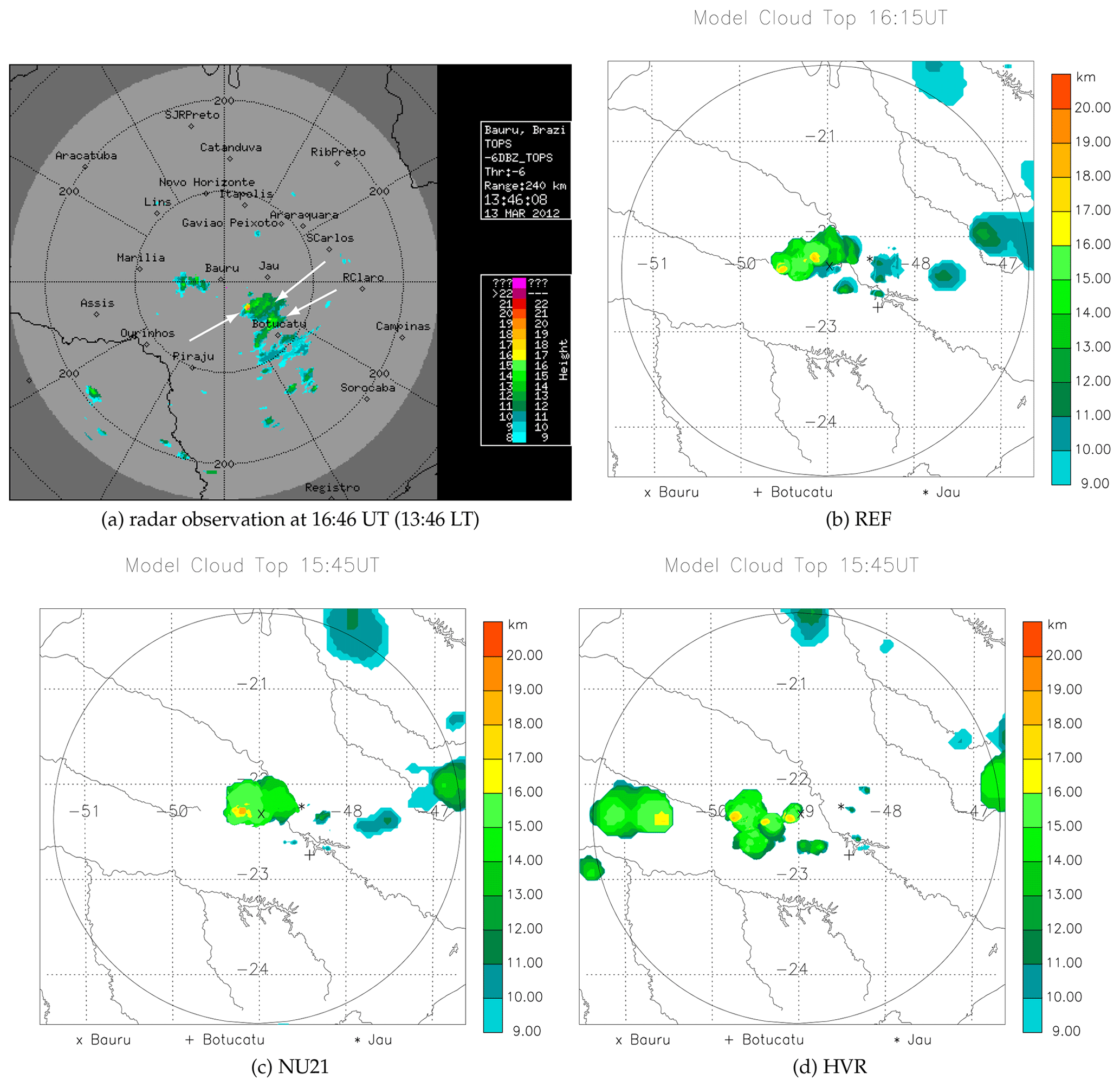
Figure 1Snapshots of echo tops, observed by the S-band radar and modelled cloud tops from the BRAMS simulations on 13 March 2012, centred at Bauru. (a) Radar observation at 16:45 UT, then (b–d) REF at 16:15 UT, NU21 at 15:45 UT, and HVR at 15:45 UT. The circle displayed in panels (b), (c), and (d) corresponds to the 240 km radar range in (a). The arrows represent the three deep convective cells that surround Botucatu, one of which has a cloud-top height greater than 18 km.
Figure 1 allows a qualitative comparison of the radar echo tops and modelled cloud tops from the three simulations. It illustrates the capacity of BRAMS to reproduce the principal features: triggering deep convection, structure evolution, and severity of the overshooting plume in this relatively unorganised convective cluster. Note that here we compare the convective plumes when they are within a 100 km radius of Bauru (the inner circle in Fig. 1a) to avoid a relatively large scanning angle of the radar and thus to obtain accurate echo top heights. Furthermore and importantly, the modelled cloud tops are well within the third grid, not near or at the edges of this grid. We observe that the model can reproduce relatively well these highly unpredictable convective systems. There exist similar deep convective clusters around Bauru in the radar images and the simulations, although at slightly different times. The radar image at 16:46 UT (13:46 local time; Fig. 1a) shows a storm cluster comprising three cells near Botucatu, southeast of Bauru with the echo top of the furthest west one reaching higher than 18 km level. We should emphasise that small cloud droplets and ice particles, which are the principal components of overshooting plumes, are considerably less sensitive to the S-band radar because they do not sufficiently fill the beam cross section. In REF (Fig. 1b), we notice a comparable convective storm complex to have developed at 16:15 UT west of Bauru, depicting two cloud tops of height greater than 17 and 18 km, respectively. At 15:45 UT, NU21 (Fig. 1c) indicates a similar convective system in the west of Bauru, as seen on the radar image (Fig. 1a) 1 h later in the southeast of Bauru, but with only one cloud top greater than 18 km level. HVR (Fig. 1d) also produces a convective cluster at 15:45 UT in the west of Bauru but comprising three cells in the vicinity of Bauru, 100 km, with two cloud tops of height greater than 17 km and one greater than 18 km.
The full time series of the comparison between the modelled cloud tops and the S-band radar echo tops is in the Supplement (animation of cloud tops) every 7.5 min from 15:01 to 18:52 UT on 13 March 2012. Figure 1 demonstrates the main features of this series of comparison at the peak of the convective activity. The radar is largely cloud free at the start of the convective activity (15:01 UT); the only convective cells are around 100 km south–southeast of Bauru near Botucatu, with tops typically at 9 to 10 km in altitude. REF reproduces this feature qualitatively with the same range of maximum height but much closer to Bauru, however, south–northwest of Bauru. The same type of storm cluster is observed in NU21 at 14:15 UT. About 45 min later, at 15:00 UT, NU21 produces convective activity triggering at the same position as in REF but with more intensity and higher cloud tops. It highlights that deep convection triggers earlier in NU21. At 14:15 UT, there is no sign of convective activities in HVR, unlike in the radar image, but it appears at 15:00 UT near Ourinhos – southwest of Bauru. The convective cells are overgrown in the area than in NU21 at 14:15 UT, though in a similar position. By 15:00 UT, the deep convection altitude in HVR is also higher than in REF and the radar echo tops. It is also located much more west than the radar observations. However, stratospheric overshoots are present in the simulations as well as in the radar observations with the echo top above 17 km at the peak of the convective activity, i.e. during 16:00–17:00 UT. In the three simulations, convective activity increases in height and spreads over larger areas in the TTL as time passes. In HVR, it is further west–southwest of Bauru. Thus, all simulations predict the onset of convective activity to be slightly earlier than observed. Given the uncertainties in modelling and S-band radar perceptions of deep convective activity, associating one-by-one simulations with radar convective cells in spatial and temporal terms is a difficult task (e.g. Li et al., 2008; Rowe and Houze, 2014; Weisman et al., 1997). As a result, it may not be the most appropriate criterion for evaluating these disorganised deep convective cloud simulations.
Table 1Count of overshoots above 17 km altitude for the S-band radar (end time UT of the volume scan) and for the REF, NU21, and HVR simulations. Their counts are represented as multiples of ×. Within a 1 km thick layer, the altitude is the lowest point. The modelled overshoots are calculated by taking into account the height of each plume in the 7.5 min time-lapse imagery, which must be greater than or equal to 17 km, as well as the spatial spread of each plume. Figure 6 depicts a scenario in which the spatial extent of the overshoot is also taken into account.
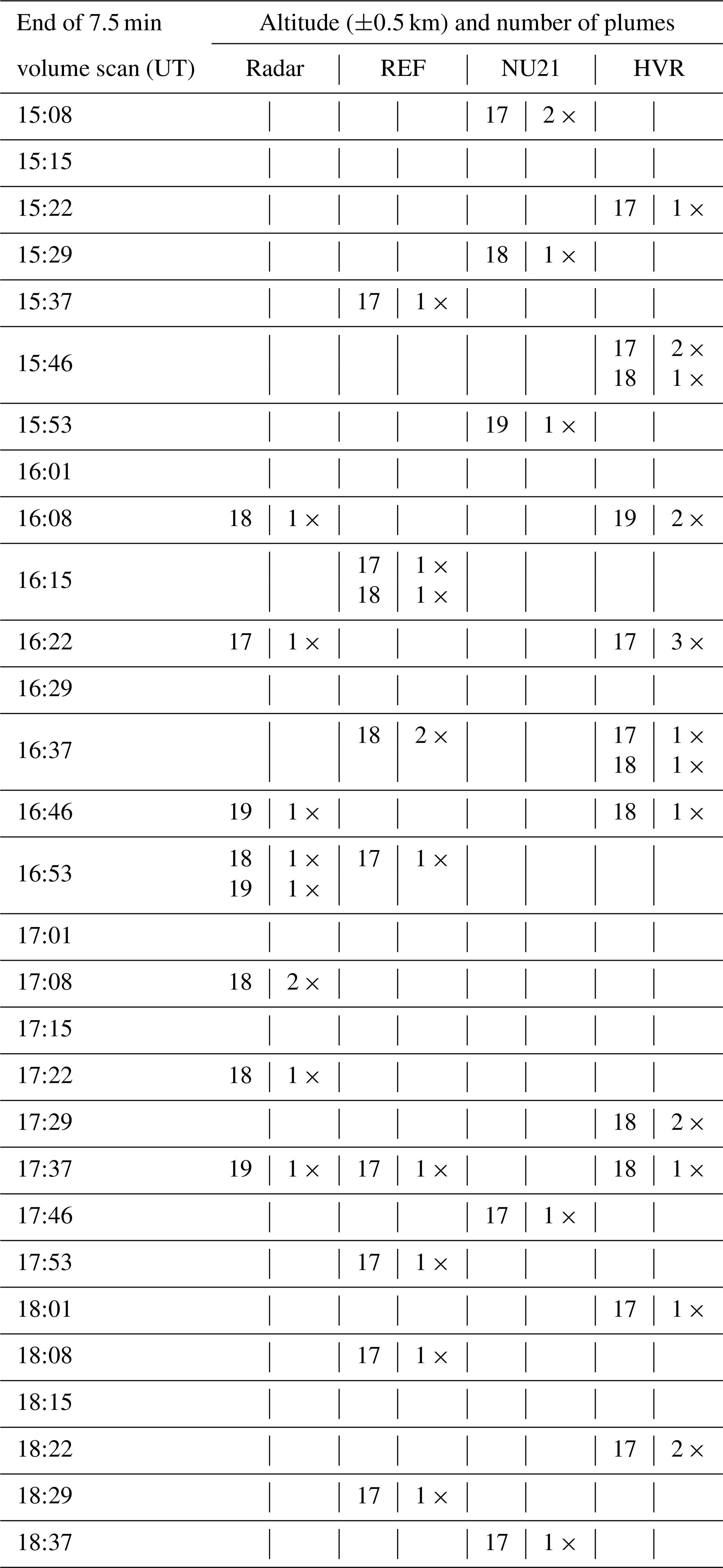
However, during the period 15:00–18:30 UT on 13 March 2012, within a 100 km radius of Bauru, we tabulate (Table 1) the number of overshooting plumes higher than 17 km altitude – the radar threshold for detecting overshoots. It is to have a general understanding and knowledge with in the three cloud-resolving simulations. The observation period is limited to 18:30 UT since the radar images reveal deep convection decaying after that time. REF can produce an equal amount of overshooting plumes observed by the S-band radar, though at somewhat higher altitudes, as shown in Table 1. We expect this because radar sensitivity to low-ice content is low, causing the radar to underestimate the number of overshoots. Furthermore, a situation in which the 380 K layer is below the 17 km altitude threshold is a reasonable explanation. The overall number of overshooting cells in NU21, on the other hand, implies that it is less favourable than REF and radar at producing overshooting plumes. The time series analysis of cloud clusters indicates that the lifetime of overshooting plumes appears to be longer than REF, where overshooting plumes rarely reach 19 km (see the animation on cloud tops in the Supplement). HVR, on the other hand, has approximately 18 overshooting plumes during the observation period, which is significantly more than REF (10 overshoots) and NU21 (6 overshoots).
To further understand the situation, one can expect HVR to determine more reliable dynamics across the tropical tropopause than REF and NU21, respectively. Contrary to expectations, it tends to intensify massive deep convection activity. A plausible fact to explain such behaviour in HVR is the ratio between vertical and horizontal grid points, which overestimates vertical motions due to grid cell saturation (Homeyer et al., 2014; Homeyer, 2015). It might be the model's Courant–Friedrichs–Levy (CFL) limit, which in finite-difference simulation techniques constrains the relationship between infinitesimal increases in space grid points and infinitesimal time step increments. In the BRAMS model, the von Neumann stability assessment (Deriaz and Haldenwang, 2020) is necessary for the transport equations related to convection. Aside from that, Eulerian model simulations of high vertical resolution, high-frequency wave motions, such as inertia–gravity waves (e.g. Staquet, 2004; Young, 2021), can be overdetermined. As a result, they can exaggerate cloud microphysics (Aligo et al., 2009) and cause erroneous cloud conditions near the TTL (Jensen and Pfister, 2004). Therefore, we leave HVR out of the next sections to describe the details, and we do not look at this simulation's water budget in the lower stratosphere.
In Sect. 4.1, we essentially outline several principal aspects by closely studying the simulated convective plumes. First, we locate the position of deep convective activity further west–northwest in the model, typically 50 to 60 km west–northwest. Second, the time evolution of the convective clusters reveals that they are moving north–northwest, while most of the convective activity remains in the west of the Tietê River in both cases. Overall, we cannot expect the model to predict precisely the position and time of convective activity development. REF and, to a certain extent, NU21 provide reasonable predictions in space and time. They generate good estimates of convective cloud tops but initiate the plumes generally earlier compared to the radar observation. In contrast, HVR yields unfavourable conditions and exaggerates its size.
4.2 Validation against TRO-Pico balloon-borne measurements
The WV and particle measurements performed in the vicinity of overshoots in the frame of the TRO-Pico campaign establish a well-documented database to validate model simulations. For our study, as the balloon-borne measurements belong to a moment several hours after the overshooting event – this time interval between the overshooting event and the balloon-borne measurements is indicated as δtom hereafter; the simulation validation strategy is as follows. We observe the modelled overshooting plume at 17.2 and 17.8 km altitudes, respectively, where FLASH-B and Pico-SDLA hygrometers captured the WV local enhancements (see Khaykin et al., 2016). Then, after the same δtom, we investigate the WV enhancement at these levels in the model.
4.2.1 REF simulation
To validate the local WV enhancement at 17.2 km altitude due to the modelled overshoots, we combine the TRO-Pico measurements by FLASH-B at 23:45 UT corresponding to an overshooting event that occurred at 16:46 UT with δtom=7 h on 13 March 2012. We observe the time evolution of the modelled (REF) overshooting plume at 17.2 km altitude from 16:15 UT to 23:15 UT to maintain the same δtom. Figure 2 illustrates the horizontal cross section of the total water content at 17.2 km altitude at three different time stamps, viz., 16:15, 19:45, and 23:15 UT, sequentially. It also draws the horizontal wind streamline to follow the direction of the moving plume at this height. We prepare this kind of plot every 7.5 min to follow the evolution of the overshooting cell at that height. For simplicity and due to space limitations, we show only these three plots in the paper.
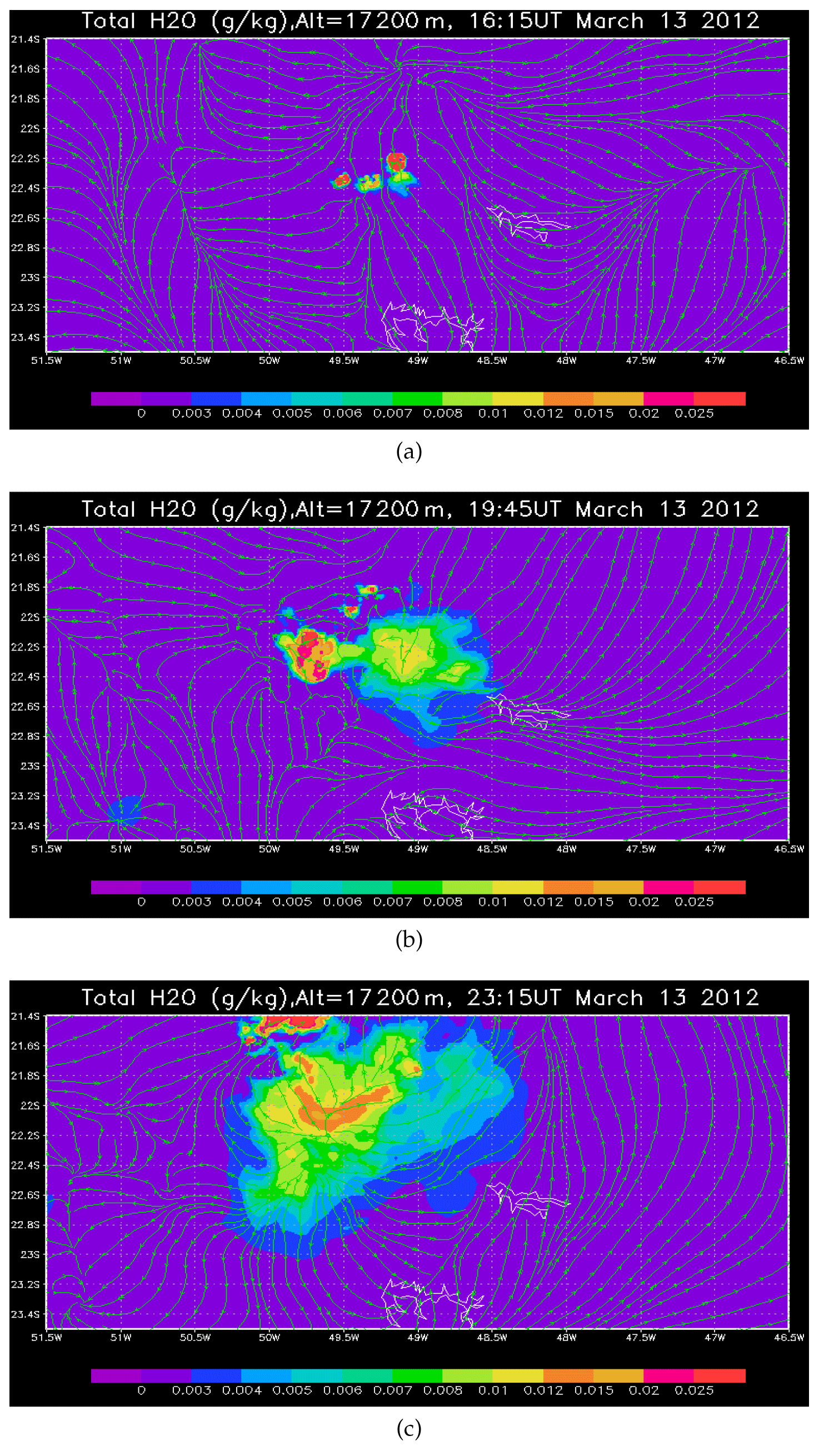
Figure 2BRAMS simulation: REF total water content, ice, liquid, and vapour in g kg−1, at 17.2 km altitude at (a) 16:15 UT, (b) 19:45 UT, and (c) 23:15 UT, respectively. The streamlines represent the horizontal wind fields within the domain, a composite of the second and third grids.
Figure 2a illustrates REF determined overshooting plume at 22.2∘ S, 49.15∘ W, entering the stratosphere at 16:15 UT. About after 3.5 h, we observe this plume spreading wide horizontally (Fig. 2b), mostly east to 49.4∘ W. Furthermore, several other overshooting plumes developed in between but did not interact with the eastern part of the convective plume. Around 23:15 UT (Fig. 2c), most of the original plume moved eastward of 49.1∘ W by advecting northward, as precisely as described in the trajectory analysis of the same case in Khaykin et al. (2016). At some positions within the overshooting plume corresponding to the maxima of H2O mixing ratio (ice, liquid, and vapour), we obtain the local enhancement is typically 2 ppmv of the total water content (see Fig. 3a) at this altitude within ±35 km northeast of Bauru.
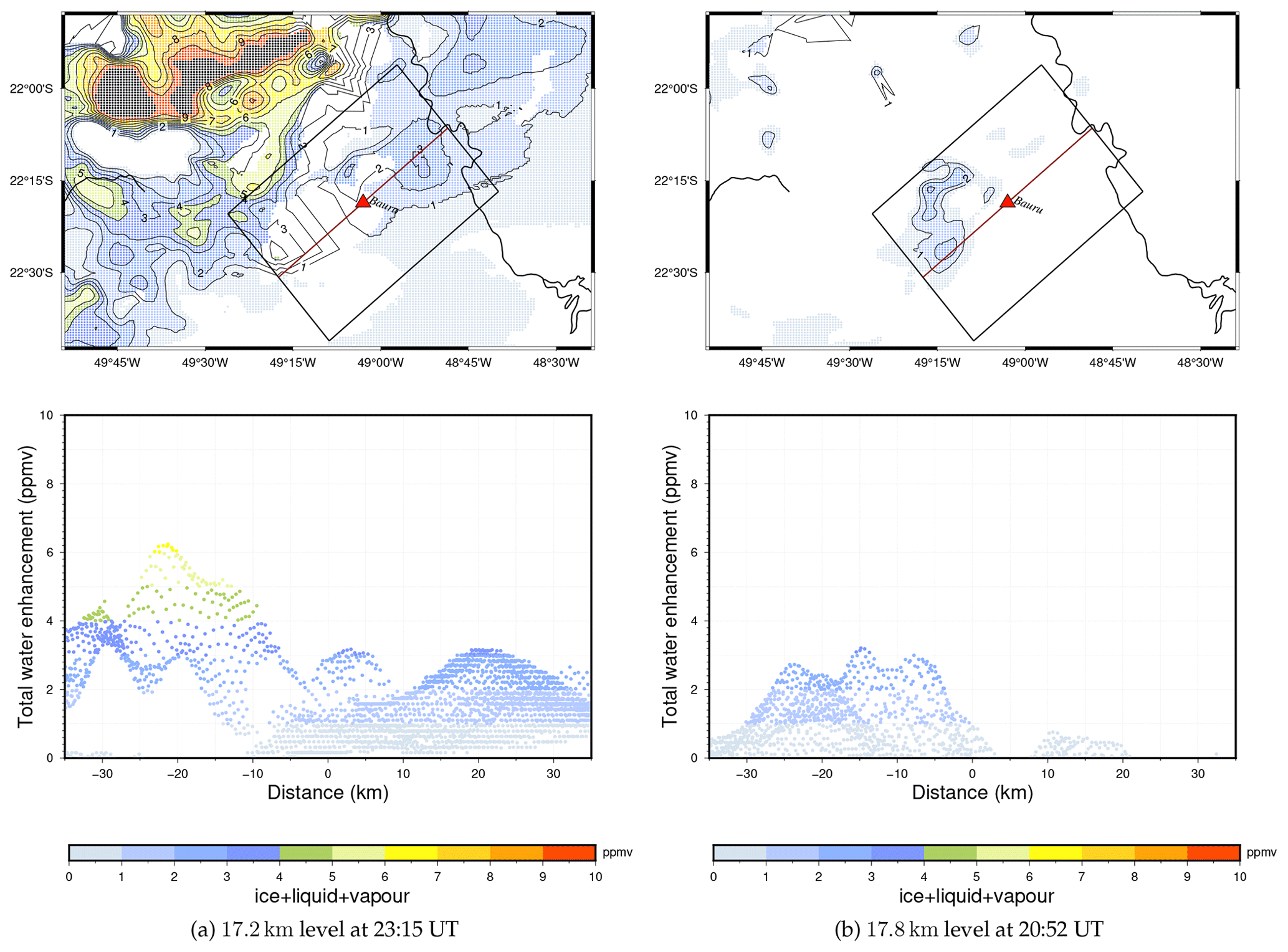
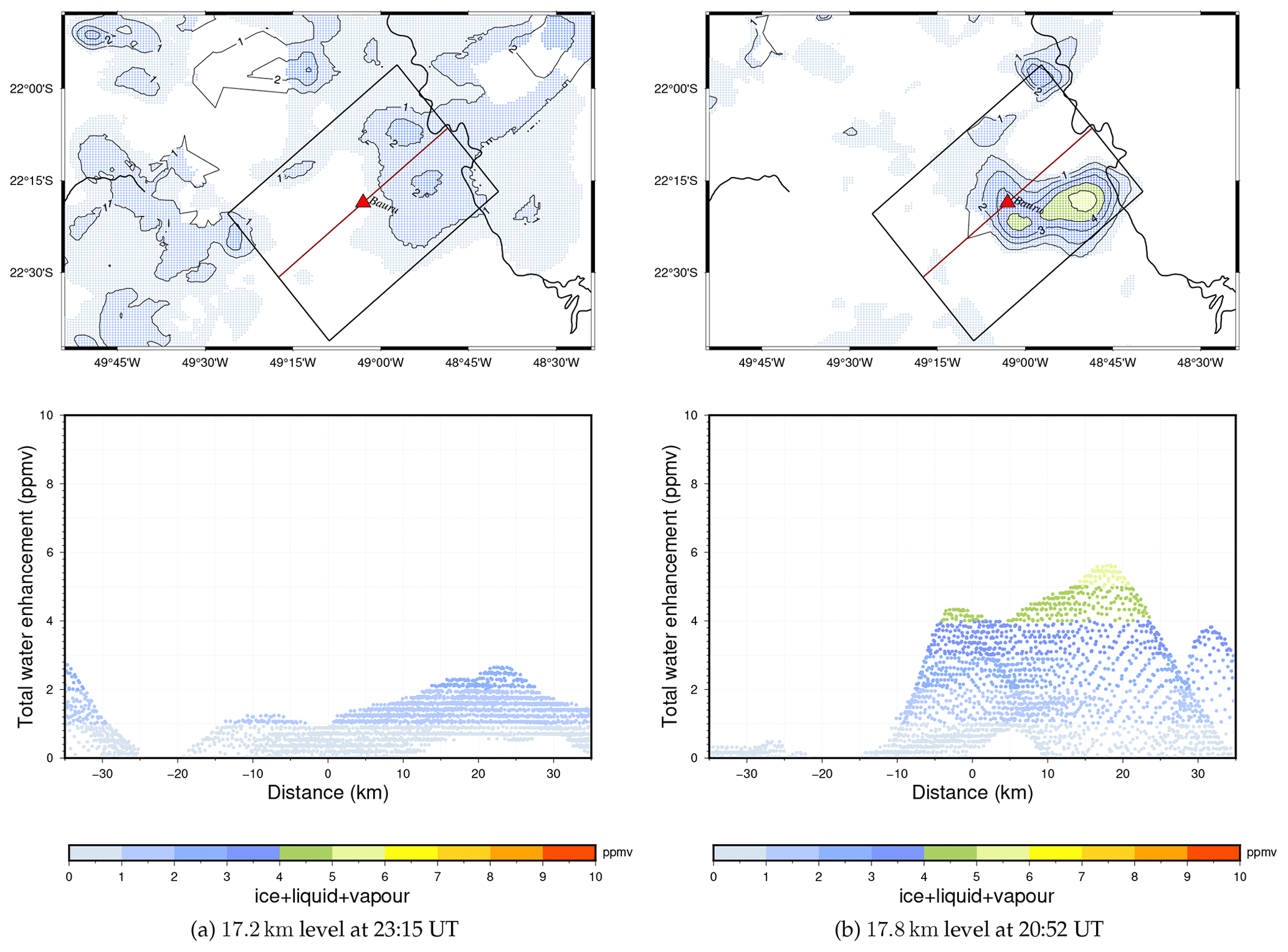
Figure 3REF providing total water (ice, liquid, and vapour) enhancement at (a) 17.2 km altitude at 23:15 UT and (b) 17.8 km altitude at 20:52 UT, respectively. The top panel shows the horizontal cross sections of the vertical grid at these altitudes, depicting the only grid points when their total water content is higher than the model levels simply above and below in a vertical column. The isolines show the enhanced total water content (ppmv) with respect to the model layer below it. The bottom panel shows the grid points'/pixels' water content confined by the northeast-tilting rectangle having the length of 70 km and half width of 25 km. The red triangle denotes Bauru (0 km); the northeast direction is positive, and vice versa.
Figure 3 highlights such H2O enhancement domains in isolines. In Fig. 3a, at 23:15 UT around Bauru within an area of 70 km × 50 km, tilting northeast following the analysis in Fig. 2, REF produces many grid points representing H2O enhancement of about 0.5 ppmv at 17.2 km altitude, which is in agreement with FLASH-B and Pico-SDLA measurements. The confirmation of no ice remaining indicates that all the ice has sublimated or sedimented in the simulation. It agrees with the measurements carried out using LOAC and COBALD under the Pico-SDLA and FLASH-B, where they did not detect any ice particles in the stratosphere. The modelled 0.5 ppmv enhancement at the 17.2 km level is comparable to the one measured by FLASH-B, 0.45 ppmv, in that range of altitude. REF also produces very high H2O enhancement, greater than 10 ppmv, in the northwest region away from Bauru. Such extremely wet conditions are possible due to a very recent overshoot in this area in the simulation.
Then, we implement the same strategy to validate the hydration due to overshoot at 17.8 km altitude; see Fig. 3b. It is the altitude of the second water enhancement captured by both Pico-SDLA and FLASH-B hygrometers. Khaykin et al. (2016) report this H2O enhancement comes from another overshooting plume than the one explaining the 17.2 km H2O enhancement. We investigate if a realistic overshooting plume in BRAMS can appear with a similar H2O enhancement following the same δtom time around Bauru. For the H2O enhancement at 17.8 km altitude identified by Pico-SDLA at 22:04 UT, the associated overshooting event occurred at 17:38 UT. This implies the δtom=4 h 26 min. Following the overshooting plume, as in Fig. 2, from 16:15–20:52 UT, REF yields a similar δtom while obtaining the H2O enhancement. REF produces many grid points/pixels with H2O enhancement of 0.7 ppmv around Bauru within an area of 70 km × 50 km. Some pixels show more than 2 ppmv of H2O enhancement. Here, it is notable that BRAMS computes no ice in this part of the plume, which is in agreement with the COBALD and LOAC measurements. The 0.7 ppmv local enhancement at 17.8 km is thus fully compatible with the one measured by Pico-SDLA, 0.65 ppmv, and by FLASH-B, 0.55 ppmv, at this altitude.
The purpose of the investigation is to witness the same order H2O enhancement in the model corresponding to the TRO-Pico campaign measurements. And the approach of selecting an area of 70 km × 50 km tilting in the northeast direction around Bauru is to consider only the H2O enhancement within this area (see Fig. 3). Furthermore, it corresponds to the point that the overshooting cells at 17.2 and 17.8 km heights, respectively, are induced by two separate overshooting plumes (Khaykin et al., 2016).
4.2.2 NU21 simulation
With the same validation approach, as in REF, we select the overshooting plume that occurred at 16:15 UT in NU21. We study the time evolution of the overshooting plume at 17.2 km altitude from 16:15 UT to (16:15 + δtom) UT, that is, 23:15 UT – δtom is 7 h from the overshooting event until the FLASH-B measurement. It is similar to that in Fig. 2 and is provided in the Supplement (Fig. S1). The plume spreads horizontally, slightly southeastward, and finally northward, where most of the original plume is north of 22.4∘ S and east of 48.8∘ W at 23:15 UT.
In Fig. 4a, the conclusions are similar to REF. The total water content at 17.2 km altitude at 23:15 UT shows an enhancement of several ppmv, up to 2 ppmv at certain positions, particularly at the core of the plume. Many pixels within 10 km neighbourhood of Bauru show the WV enhancement of half a ppmv near the border of the overshooting plume. It is compatible with the local enhancement measured by FLASH-B at 17.2 km height. Moreover, it is crucial to recall the evidence of no ice remaining at this level, and the total H2O is only in the vapour phase as observed by the LOAC particle counter and the COBALD backscatter sonde. Then, we analyse the WV enhancement in NU21 at 17.8 km altitude at 20:52 UT, that is δtom=4 h 40 min after the 16:15 UT overshooting event (see Fig. 4b). This δtom is the same as the time interval between the Pico-SDLA measurement and the overshooting event. In Fig. 4b, we obtain many pixels, located at the border of the overshooting plume, with a ∼0.7 ppmv H2O enhancement without any ice remaining – a very similar way of observation to that by Pico-SDLA and LOAC. Furthermore, there are many pixels near the Tietê River giving very high WV enhancement, up to 6 ppmv. This sort of large water enhancement from overshoots has already been identified by the FISH hygrometer aboard the Russian M-55 Geophysica high-altitude aircraft in the SCOUT-AMMA field campaign in west Africa (see Schiller et al., 2009). It is now reasonable to state that BRAMS simulated overshooting plumes responsible for the local WV enhancements; however, these were not necessarily exactly in the same locations as the observed ones. Moreover, the wind spreading about the overshooting plumes is somewhat different from that in the realised ones during the TRO-Pico field campaign.
4.3 Conclusion of the validation
In Sect. 4.2, we demonstrate that the BRAMS model, via REF and NU21, can simulate fairly realistic deep convective plumes that are compatible with the IPMet S-band radar observation during the temporal evolution of deep convective cloud systems over three hours. However, these modelled deep convective plumes slightly west–northwest of the radar observation but with an intensity comparable to the detected ones by the S-band radar. Furthermore, the convective cloud tops are sometimes higher in altitude than the radar images. It corresponds to a possible fact that the S-band radar is a little sensitive to the ice hydrometeors – the main component of overshooting plumes addressed in subsequent sections. The number of overshooting plumes above 17 km is comparable both in the model and the S-band radar images until 18:30 UT, after which the model exhibits convective activity with a longer lifetime. The study of overshooting plumes at 17.2 and 17.8 km altitude, respectively, and the corresponding total water enhancements after ∼4.5 and 7 h, respectively, agree with both the balloon-borne measurements of H2O mixing ratio by Pico-SDLA and FLASH-B hygrometers. Moreover, note that the grid points showing several ppmv of total H2O enhancement are often at the edge of the overshooting turret – coherent with the trajectory analysis of Khaykin et al. (2016), reporting that the air masses sampled by the balloons are at the edge of the plume coming from the overshoot.
Thus, this study brings to the fore that fine-scale simulations using the BRAMS model can reproduce the overshooting convection. Both REF and NU21 can lead now to more insight into the overshooting plumes within unorganised deep convective plumes. Certain standard features like the amount of ice injection, width and surface area of the plume, H2O mass flux, and the lifetime of the active cell, which we cannot directly measure with the current available resources, both REF and NU21, can now provide more insight into overshooting plumes within unorganized deep convective plumes. In the subsequent sections, we give a quantitative interpretation of the overshooting plumes from REF and NU21. Unfortunately, HVR appears to produce excessively severe convective activity, making it unsuitable for further analysis.
We provide the five conceivable combinations of hydrometeors inside an overshooting plume to document the quantitative information collected from the simulations on the structural characteristics of a typical overshooting plume. Its base is at the 380 K isentropic level, which is the stratosphere's lowest layer. At the 380 K isentropic level, the instantaneous mass flux of individual hydrometeors is also estimated. Between the 380 and 430 K isentropic levels, it comprises the estimation of total ice mass and the five types of ice particles. Finally, a table provides the quantities that could lead to a road map of a nudging scheme of the water vapour enhancement in the lower stratosphere due to overshoots in large-scale simulations, which could lead to the quantification of the influence of overshoots on a large scale.
5.1 Structure and composition of overshoots
We assess all the five types of ice hydrometeors during an overshooting event. The series of plots in Fig. 5 represents the horizontal cross section of the ratio of different ice hydrometeors over the net ice varying with altitude around the TTL in the vicinity of the overshooting event that occurred at 16:15 UT in REF (see Table 1). We present this calculation from 15:00 to 18:52 UT for REF and NU21, which can be found in the animation of horizontal cross sections in the Supplement.
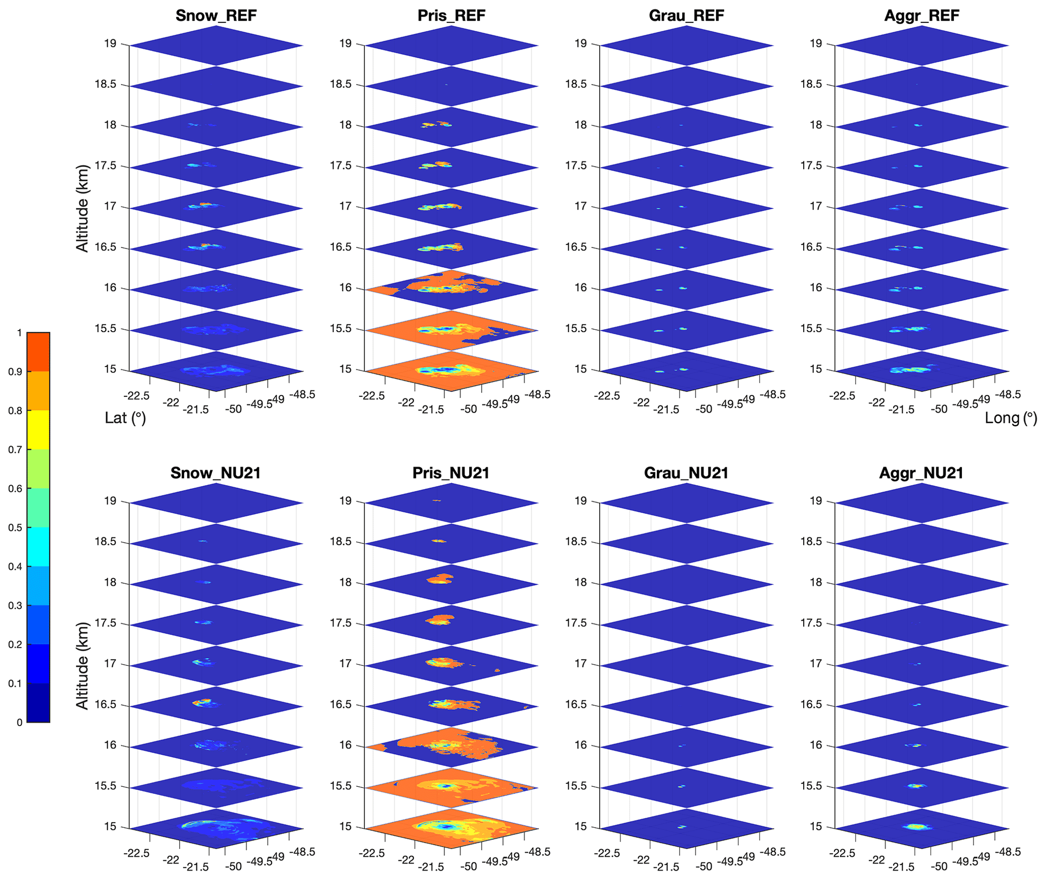
Figure 5Vertical distribution of horizontal cross section of hydrometeors, viz., snow, pristine ice, graupel, and aggregates, within the third grid, spanning over 15–19 km altitude. It is for the ratio of four types of ice hydrometeors against the entire ice content from REF – upper panel, and NU21 – lower panel, shown at 16:15 UT. Hail is not included because of its negligible values within the plume.
Above the tropopause, we find pristine ice and snow to be the primary ice hydrometeors (∼16.6 km altitude). However, aggregates and a trace amount of graupel are present. It is only true for REF. The full time evolution of the horizontal cross section can be found in the Supplement. The lack of this in NU21 could be attributed to its microphysical configuration, which allows larger hydrometers to be placed deeper within the convective plumes, resulting in a lower convective updraft and inability to reach the tropopause layer. This is evident in Table 2 and Sect. 6.1, where REF is shown to release approximately 10 % more ice with a relatively higher flux rate at 380 K isentrope than NU21. Furthermore, as expected at this level, the presence of hail particles is negligible, as shown in Fig. 5, which confirms the results of Homeyer and Kumjian (2015), obtained using S-band radar measurements of deep convective activity over the extratropics. It is consistent with the results reported in Chemel et al. (2009). Using the WRF model, they investigate the Hector thunderstorm and find (pristine) ice and snow as the primary components. However, the current study makes use of the BRAMS model, which combines five types of ice hydrometeors rather than three in the WRF version used by Chemel et al. (2009). Within the overshooting plume, Fig. 5 also reveals a large amount of aggregates and graupel at the tropopause level, particularly for REF. It is worth noting that pristine ice is completely absent towards the plume's deepest core at the base (16.6 km height, ∼380 K). Snow, aggregates, and, to a lesser extent, graupel are the only hydrometeors that survive. The major ice hydrometeors in NU21 are snow particles, which disperse across a small area with a radius of around 5 km. The overshooting dome at the edge of the plume near the tropopause level in all three scenarios is entirely formed of pristine ice. In both scenarios going up to 18 km, well into the stratospheric region of the TTL, only pristine ice (70 %) and snow (30 %) are the principal constituents of the overshooting dome. Graupel and aggregates are present in REF but not in NU21. This finding is in line with sensitivity tests conducted by manipulating microphysics in Chemel et al. (2009) and Wu et al. (2009), who used the WRF model to investigate convective updrafts during the monsoon over Darwin, Australia. Our model illustrates an overshooting plume's overall particle distribution as well as its thermodynamic structure, which is controlled by particle size distribution and affects the convective updraft.
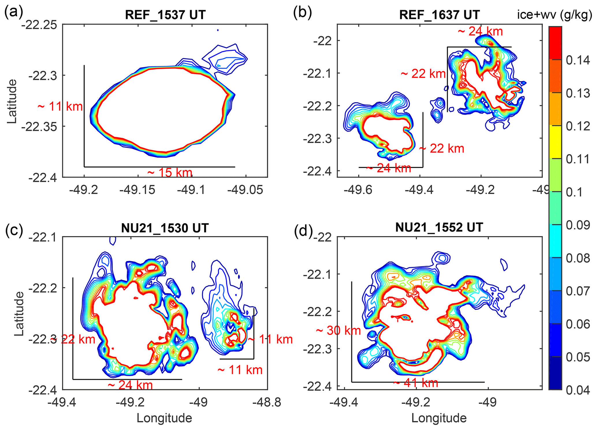
Figure 6Size of the overshooting plumes at the 380 K isentropic level, shown for REF (a, b) at 15:37 UT and 16:37 UT, and NU21 (c, d) at 15:30 and 15:52 UT, respectively. These times are selected from Table 1. The colour contours show certain levels from 0.04 to 0.14 g kg−1 of total H2O content to highlight the outer part of the overshooting plumes. The solid black lines give the approximate range of each figure in kilometres.
The contact area or spreading (km2) of the overshooting plume at the lowest layer of the stratosphere, i.e. the 380 K isentropic level, is then determined. Figure 6 depicts the spreading of overshooting plumes at this level for REF and NU21 at various time steps as shown in Table 1. The average surface area of the propagation of the overshooting plume at 380 K level is about 450 km2, according to Fig. 6. It is roughly the grid-point resolution of a large-scale simulation (400 km2), where Behera et al. (2018) show that with such horizontal grid-point resolution, BRAMS cannot explicitly produce overshoots, and illustrate the TTL dynamics and WV variability at a continental scale during a full wet season. In a cloud-resolving-scale simulation, BRAMS generates overshoots that spread over 450 km2 in the area at 380 K level, expanding from the third grid to the mother grid to disclose the intensity of convection. Hence, it is a critical point to consider when planning an overshoot nudging scheme.
Furthermore, we compare the horizontal spreading between REF and NU21. In Fig. 6, the upper panel represents the surface areas of REF, which are of 11 km × 15 km at 15:37 UT and 22 km × 24 km at 16:37 UT, respectively. In the case of NU21, the lower panel, the surface areas are of 22 km × 24 km and 11 km × 11 km at 15:30 UT, and 30 km × 41 km at 15:52 UT, respectively. The latter one with the large surface area indicates that changes in the particle size distribution, the shape parameter ν, may modulate the spreading of overshooting convection while penetrating the stratosphere. In the following sections, we estimate the mass budget corresponding to UTLS, set as a preferred range of isentropic levels.
We estimate each hydrometeor's instantaneous mass-flux rate across the 380 K isentropic level. The rates are the average over the domain that comprises only the third grid of simulation. Please note that it is not representative of a property of any particular overshooting plume but preferably addresses a realistic estimation on the flux rates of ice particles entering the 380 K isentropic layer. Besides, we evaluate the net H2O mass budget prevailing within the slice of 380 to 430 K isentropic levels.
6.1 Mass flux across the 380 K isentropic level
Figure 7 presents the domain-average instantaneous mass-flux rate for REF and NU21 across the 380 K isentropic level over the third grid of the simulation during 14:00–18:52 UT. It depicts primarily the inferences drawn from Fig. 5. Such as the principal hydrometeors are pristine ice and aggregates and to a much lower amount of snow and graupel, where the order of magnitude of the maximum mass-flux rate of snow and graupel is about 4-fold smaller than the maximum of pristine ice and aggregates. Despite the non-negligible mass-flux rate of graupel, its ratio in the structure of the overshooting turret remains modest. It occurs approximately 10 % of the composition of overshooting plume in a limited area only in REF exceeding the tropopause level (∼16.6 km). Then, we associate the contrast in the snow composition inside the plume with the sedimentation. Graupel, denser than snow, falls faster to the troposphere, results in the accumulation of snow in the stratosphere. Though the overshoots begin at different times in REF and NU21, the local maximum of mass-flux rates are of the same order of magnitude, and in REF, it is regularly higher than NU21. It is already explicit that the number of overshooting events is different in REF and NU21 (please refer to Table 1). Eventually, the differences in the mass-flux rate between REF and NU21 would be critical to explain as their values are also proportional to the vertical wind velocity (see Sang et al., 2018).

Figure 7The instantaneous domain-average mass-flux rate (g m−2 s−1) of each hydrometeor and water vapour is illustrated in the third grid of the simulations for REF (green) and NU21 (blue). The cosine component of the vertical velocity with respect to the horizontal is used to determine the upward flux rate, which takes into account the slope at the 380 K level due to deep convection.
6.2 Mass budget above the 380 K isentropic level
Figure 8 depicts the total mass budget (kilotonne, kt) for the five types of ice hydrometeors: pristine ice, snow, aggregates, graupel, and hail, as well as water vapour. It is worth mentioning that the amount of liquid in this calculation has no bearing. The simulations' third grid, which has a domain size of 201 km × 165 km and isentropic values ranging from 380 to 430 K, is used for time-integrated estimation. Because none of the convective plumes in the simulations exceed this isentropic level, the maximum level is 430 K. Our mass budget estimation begins with an unperturbed state (zero total mass), i.e. the time before deep convection begins in each simulation, which is 15:00 UT for REF and 14:00 UT for NU21, respectively, and ends at 17:30 UT for both. This is because the WV time evolution reaches a near-plateau profile without including any further overshoots, which would otherwise make the study more difficult. Furthermore, the ice profile (dotted red) is descending, indicating that deep convection activity in the model has ended. Simultaneously, the WV profile (dotted blue) rises and settles around 17:30 UT.

Figure 8Water mass budget (ice and water vapour) for (a) REF and for (b) NU21 in the third grid between the 380 and 430 K isentropic levels. The ice budget contribution includes the five ice hydrometeors (pristine ice, snow, aggregates, graupel, and hail). The colour and length of the arrows indicate the cloud-top altitude of each occurrence, with the smallest arrows (brown) referring to cloud-top heights of 17–18 km, the intermediate-sized arrows (green) relating to cloud-top heights of 18–19 km, and the largest arrows (magenta) corresponding to cloud-top heights greater than 19 km.
In both simulations, the total H2O (ice and vapour) mass budget estimations with respect to the unperturbed state show a net increment of 8 kt accumulated over 17:30 UT. In contrast, the vapour increment due to overshoots is only 2 kt in REF and 3 kt in NU21. The difference in vapour enhancement is attributed to the simulations' different particle size distribution, implying a variation in the sedimentation process. Another interesting fact is that NU21 has a longer lifetime than REF since the last overshoot above 17 km. As a result, ice particles injected into the stratosphere in NU21 should have a longer time to sublimate than ice particles injected into the stratosphere in REF.
In REF, we explain the peak of total water content at 16:22 UT with the last two overshooting events that occurred at 16:15 UT (refer to Fig. 8a and Table 1) injecting a bulk amount of H2O remaining in the lower stratosphere. We observe two more events occurring at 16:37 UT, causing a modest enhancement in the total water mass. Subsequently, the last overshooting event at 16:52 UT is not significant enough to add H2O to the lower stratosphere. Now, in NU21, the triggering time of the overshooting events is different than REF, where we observe several peaks in Fig. 8b during 15:00–16:37 UT. Recalling the results in Table 1, it does not produce as many overshoots as REF during the period of observation, although it represents more intense overshoots reaching higher than 19 km. Besides, the rise in total H2O values after a decline at 16:15 UT is possible because of other new overshoots, overpassing the 380 K layer, but not recognised due to the lower height below the threshold level of 17 km.
Moreover, we determine the standard amount of hydration for each overshoot, providing both the upper and lower limits by reflecting the two extreme cases on the fate of ice. As such, (1) the upper limit would assume all the remaining ice sublimates in the stratosphere, and (2) the lower limit would indicate all the remaining ice is falling back to the troposphere without sublimating at all. The upper limit is about 8 kt6 ≈ 1.34 kt in REF, whereas it is 8 kt4 = 2 kt in NU21. The lower limit of hydration for REF is 2 kt6 ≈ 0.34 kt, whereas for NU21, it is 3 kt4 ≈ 0.75 kt. In both the cases during 15:00–17:30 UT, the denominator denotes the total number of overshooting turrets, denoted by arrows in Fig. 8, and the numerator gives the net amount of WV enhancement. The lower limit is an important point, which is unlikely to be reached because of the very weak fall speed of the small size pristine ice and snow particles.
Figure 8 also confers some information on the total amount of ice injected by an individual overshooting plume. For REF at 15:37 UT, we observe ∼2 kt of ice enhancement because of one overshooting plume and later at 16:15 UT, ∼11 kt because of two more overshoots. The contribution of one overshooting event is thus 13 kt3 ≈ 4.3 kt of ice only. Following the identical strategy for NU21 at 15:07 UT, the ice enhancement due to single overshooting event is 8 kt2 = 4 kt. Several mesoscale modelling studies (e.g. Liu et al., 2010; Lee et al., 2019) and satellite observations (e.g. Iwasaki et al., 2010; Lelieveld et al., 2007) have already reported this type of total water enhancement due to overshoots in the tropical lower stratosphere. Dauhut et al. (2015) estimate about 2.78 kt of WV enhancement, and Lee et al. (2019) estimate a water budget of 0.87 kt. Our calculations, 1.34 kt in REF and 2.0 kt in NU21, are within the range of these studies and are of the same order of magnitude. However, this calculation is significantly higher than the estimation of Liu et al. (2010), ∼0.5 kt at maximum, where they use the same version of the BRAMS model to analyse the overshoots occurring in west Africa, but is less constrained by observations. On the other hand, Dauhut et al. (2018) provide the estimation of the individual contributions of each overshooting plume hydrating the stratosphere, leading to a lower estimate. However, the method applied to get this estimation is absent. Overall, our estimations of the total H2O enhancement are compatible with most of these studies. They could pave the way for forcing the impact of overshoots in a large-scale cost-effective computing simulation, which cannot resolve overshoots due to coarser horizontal representation.
To get quantitative information on the mass distribution of five different types of ice hydrometeors within the overshooting plumes constrained within the thin layer of 380 to 430 K isentropes (see Fig. 5), we estimate the percentage of each type of ice particles. It follows in two ways: (1) , where mi corresponds to the mass of a particular type of ice particles i within a layer of 380 to 385 K, and Mi corresponds to the mass of the same type of ice particles i within a layer of 380 to 430 K; (2) we express them as a percentage of the mass of a given kind of ice particle to the total mass M of ice particles, , within a layer of 380 to 430 K, namely, . We tabulate the results in Table 2.
Table 2Mass (%) of individual ice hydrometeors within the 380 to 385 K isentropic layer (ρ1) and 380 to 430 K isentropic layer (ρ2), respectively, with respect to its total ice mass within the 380 to 430 K isentropic layer. Results are tabulated for four different cases: the first two rows for REF and the rest for NU21.

One of the major inferences drawn from Table 2 is the amount of ice injected by various overshooting plume remaining within a layer of 380 to 385 K, ρ1: ∼72 % in REF and ∼65 % in NU21. The ρ1 and ρ2 highlight the conclusions of Sect. 5.1; i.e. the overshooting plume is essentially comprised of pristine ice, snow, and aggregates, though it can contain a small amount of graupel, present mostly at 380 to 385 K, the base of the plume. Furthermore, within 380 to 430 K, hail is negligible in the overshooting plume for both of the simulations but is always the dominant hydrometeor in the base of the plume, featuring the results of radar observations in Homeyer and Kumjian (2015). We also recognise competition in the growth of pristine ice over aggregates and graupel concurrently within the plume. Whenever aggregates and graupel are relatively large in mass inside the plume, e.g. 15:37 UT in REF and 15:30 UT in NU21, pristine ice prevails relatively low, and vice versa, e.g. 16:37 UT in REF and 15:52 UT in NU21. It signifies the existence of the weak vertical velocity, which results in settling back of larger particles. Thus, hail and graupel fall back to the troposphere, allowing further growth of smaller ice particles (see Homeyer and Kumjian, 2015; Qu et al., 2020) in the lower stratosphere within an environment comprising a significant quantity of supercooled liquid water content. In Table 2, the variations in the quantities of individual ice particles above 380 K layer between the two simulations are possibly due to the small change in the microphysics adopted to investigate the impact of shape parameter (ν) on producing overshoots. Since the ν value is higher in NU21, the particle size distribution is more limited than in REF. The particle size distribution resulting from a gamma function becomes narrower as the ν value increases (see Eq. 1). Consequently, the lesser variability present in the particle size distribution of NU21 could lead to a more efficient falling back process of larger ice particles to the troposphere in comparison to REF. Besides, recalling the results from Fig. 8, the longer prevalent behaviour of overshoots above 17 km in NU21 than REF could lead to higher sublimation of ice in NU21 confirms our observation of less injection of ice in NU21 to the lower stratosphere but results in more hydration.
This paper describes several cloud-resolving simulations of convective overshoots penetrating the lower stratosphere using the BRAMS mesoscale model, corresponding to an observed case on 13 March 2012, during the TRO-Pico field campaign in Bauru, Brazil. During this series of overshooting convection events, several plumes reached the stratosphere. As a result, it accounts for the hydration heterogeneity produced by overshoots of variable intensity, even when they occur under similar circumstances (e.g. stratospheric humidity). The S-band radar stationed at Bauru, as well as the balloon-borne measurements from this campaign, allow the simulation results to be validated. These simulations, which have been validated as realistic when compared to TRO-Pico measurements, are then used to obtain the main physical characteristics of overshooting plumes.
The main results are as follows.
-
Primarily, the simulated overshooting plume reaching the lower stratosphere comprises pristine ice and snow, and to some degree aggregates but only at the base, the 380 K isentropic level.
-
The cross section of the overshoots at the 380 K isentropic level is about 450 km2, and interestingly, it is close to the mother grid resolution, 20 km × 20 km, at which BRAMS cannot determine explicitly the overshooting convection (see Behera et al., 2018).
-
Within the limited layer of 380 to 385 K, 68 % of the overall ice mass exists. It also suggests that the remaining 32 % of ice (mostly pristine ice and snow) moves higher in the stratosphere. Because of the very slow fall speed at altitudes above 385 K and the subsaturated conditions with respect to ice, that 32 %, which is pristine ice and snow, is anticipated to stay in the stratosphere and sublimate.
-
A single overshooting plume injects around 4.3 kt of ice in REF and 4.0 kt of ice in NU21 over the 380 K level in this given scenario in Bauru, with NU21 injecting slightly less ice than REF as expected.
-
The stratospheric WV enhancement due to one overshooting event is estimated to range between 1.34–2 kt as the upper limit and 0.34–0.75 kt as the lower limit after sublimation and (or) sedimentation of the stratospheric ice. If we consider complete sublimation of ice, as in REF, it confirms our estimate that the 32 % of 4.3 kt of ice irreversibly travelling further up to the stratosphere results in the stratosphere having the lowest hydration in the upper limit range.
These data can be utilised to develop a nudging method that quantifies the influence of overshooting convection on the stratospheric water vapour using a low-cost large-scale simulation. Though the findings are limited to a case study in Brazil and may not be generalisable, more similar case studies should be conducted in order to gain a better knowledge of the events, and this work is keeping with that goal. This instance would be the next stage in the current research, offering a road map for extending the impact of overshooting convection on stratospheric water vapour on a continental (Brazilian) scale.
All TRO-Pico measurements are publicly available at https://cds-espri.ipsl.upmc.fr/etherTypo/index.php?id=1671&L=1 (ESPRI Aeris, 2022). S-band radar data can be provided upon request to Emmanuel D. Rivière. The BRAMS model setup is publicly available at http://brams.cptec.inpe.br/ (BRAMS, 2022).
Two videos are provided for the time series analysis made every 7.5 min in the Supplement: one for the modelled cloud tops and corresponding S-band radar echo tops; the second one for the vertical distribution of horizontal cross section of different hydrometeors within the overshooting plume. The supplement related to this article is available online at: https://doi.org/10.5194/acp-22-881-2022-supplement.
EDR and AKB conceptualised the study design, methodology, validation, and analysis. JB provided the support to run BRAMS in different high-performance computing (HPC) machines, and EDR provided the resources to achieve the simulations. AKB and EDR wrote the original draft, and all authors reviewed the paper. EDR and VM received the funding for this research. SMK provided the FLASH measurements, and MG provided the Pico-SDLA measurements. GH provided the meteorology and interpretation of S-band radar data. All authors have read and agreed on the published version of the paper.
The contact author has declared that neither they nor their co-authors have any competing interests.
Publisher’s note: Copernicus Publications remains neutral with regard to jurisdictional claims in published maps and institutional affiliations.
This study is based on a case observation of the TRO-Pico campaign. TRO-Pico is a French ANR-funded project (https://anr.fr/Project-ANR-10-BLAN-0609, last access: 14 January 2022), in collaboration with the IPMet institute (Meteorological Research Institute) in Bauru, state of São Paulo, Brazil. We acknowledge the entire technical team of IPMet that helped with balloon launches. The project LEFE (Les Enveloppes Fluides) “Overshoot à Grande Echelle” also provided funding for this work. Computational resources were granted by CINES under the GENCI (Grands Equipements Nationaux de Calcul Intensif) project (nos. A0010105036, A0030105036, and A0090105036) and by ROMEO of Université de Reims Champagne-Ardennes. In the paper, we use the information that ice was not detected by LOAC (PI: Jean-Baptiste Renard at LPC2E, CNRS and Université d'Orléans, France) and by COBALD (PI: Frank Gunther Wienhold at Institut für Atmosphäre und Klima, ETH Zürich, Switzerland). Both of them are acknowledged. Finally, we want to thank the three anonymous reviewers who provided valuable feedback that helped us improve this paper.
The article processing charges for this open-access publication were covered by the Centre National de la Recherche Scientifique (CNRS)'s LEFE-IMAGO project “Parashoots”.
This paper was edited by Timothy J. Dunkerton and reviewed by three anonymous referees.
Aligo, E. A., Gallus, W. A., and Segal, M.: On the impact of WRF model vertical grid resolution on Midwest summer rainfall forecasts, Weather Forecast., 24, 575–594, https://doi.org/10.1175/2008WAF2007101.1, 2009. a
Behera, A. K., Rivière, E. D., Marecal, V., Rysman, J. F., Chantal, C., Sèze, G., Amarouche, N., Ghysels, M., Khaykin, S. M., Pommereau, J. P., and Held, G.: Modeling the TTL at Continental Scale for a Wet Season: An Evaluation of the BRAMS Mesoscale Model Using TRO-Pico Campaign, and Measurements From Airborne and Spaceborne Sensors, J. Geophys. Res.-Atmos., 123, 2491–2508, https://doi.org/10.1002/2017JD027969, 2018. a, b, c, d
Betts, A. and Miller, M.: A new convective adjustment scheme. Part II: Single column tests using GATE wave, BOMEX, ATEX and arctic air-mass data sets, Q. J. Roy. Meteor. Soc., 112, 693–709, https://doi.org/10.1002/qj.49711247308, 1986. a
Brabec, M., Wienhold, F. G., Luo, B. P., Vömel, H., Immler, F., Steiner, P., Hausammann, E., Weers, U., and Peter, T.: Particle backscatter and relative humidity measured across cirrus clouds and comparison with microphysical cirrus modelling, Atmos. Chem. Phys., 12, 9135–9148, https://doi.org/10.5194/acp-12-9135-2012, 2012. a
BRAMS: Welcome to the Brazilian developments on the Regional Atmospheric Modeling System, BRAMS [code], available at: http://brams.cptec.inpe.br/, last access: 14 January 2022. a
Brewer, A.: Evidence for a world circulation provided by the measurements of helium and water vapour distribution in the stratosphere, Q. J. Roy. Meteor. Soc., 75, 351–363, https://doi.org/10.1002/qj.49707532603, 1949. a
Carminati, F., Ricaud, P., Pommereau, J.-P., Rivière, E., Khaykin, S., Attié, J.-L., and Warner, J.: Impact of tropical land convection on the water vapour budget in the tropical tropopause layer, Atmos. Chem. Phys., 14, 6195–6211, https://doi.org/10.5194/acp-14-6195-2014, 2014. a
Chaboureau, J.-P., Cammas, J.-P., Duron, J., Mascart, P. J., Sitnikov, N. M., and Voessing, H.-J.: A numerical study of tropical cross-tropopause transport by convective overshoots, Atmos. Chem. Phys., 7, 1731–1740, https://doi.org/10.5194/acp-7-1731-2007, 2007. a
Chemel, C., Russo, M. R., Pyle, J. A., Sokhi, R. S., and Schiller, C.: Quantifying the imprint of a severe Hector thunderstorm during ACTIVE/SCOUT-O3 onto the water content in the upper troposphere/lower stratosphere, Mon. Weather Rev., 137, 2493–2514, https://doi.org/10.1175/2008MWR2666.1, 2009. a, b, c, d
Corti, T., Luo, B. P., De Reus, M., Brunner, D., Cairo, F., Mahoney, M. J., Martucci, G., Matthey, R., Mitev, V., Dos Santos, F. H., and Schiller, C.: Unprecedented evidence for deep convection hydrating the tropical stratosphere, Geophys. Res. Lett., 35, L10810, https://doi.org/10.1029/2008GL033641, 2008. a
Cotton, W. R., Pielke Sr, R. A., Walko, R. L., Liston, G. E., Tremback, C. J., Jiang, H., McAnelly, R. L., Harrington, J. Y., Nicholls, M. E., Carrio, G. G., and McFadden, J. P.: RAMS 2001: Current status and future directions, Meteorol. Atmos. Phys., 82, 5–29, https://doi.org/10.1007/s00703-001-0584-9, 2003. a
Danielsen, E. F.: A dehydration mechanism for the stratosphere, Geophys. Res. Lett., 9, 605–608, https://doi.org/10.1029/GL009i006p00605, 1982. a
Dauhut, T., Chaboureau, J.-P., Escobar, J., and Mascart, P.: Large-eddy simulations of Hector the convector making the stratosphere wetter, Atmos. Sci. Lett., 16, 135–140, https://doi.org/10.1002/asl2.534, 2015. a, b
Dauhut, T., Chaboureau, J.-P., Haynes, P. H., and Lane, T. P.: The mechanisms leading to a stratospheric hydration by overshooting convection, J. Atmos. Sci., 75, 4383–4398, https://doi.org/10.1175/JAS-D-18-0176.1, 2018. a
Deriaz, E. and Haldenwang, P.: Non-linear CFL Conditions Issued from the von Neumann Stability Analysis for the Transport Equation, J. Sci. Comput., 85, 1–17, https://doi.org/10.1007/s10915-020-01302-0, 2020. a
ESPRI Aeris: TRO-pico: overview, ESPRI Data Centre [data set], available at: https://cds-espri.ipsl.upmc.fr/etherTypo/index.php?id=1671&L=1, last access: 14 January 2022. a
Folkins, I., Loewenstein, M., Podolske, J., Oltmans, S. J., and Proffitt, M.: A barrier to vertical mixing at 14 km in the tropics: Evidence from ozonesondes and aircraft measurements, J. Geophys. Res.-Atmos., 104, 22095–22102, https://doi.org/10.1029/1999JD900404, 1999. a
Forster, P. M. D. F. and Shine, K.: Assessing the climate impact of trends in stratospheric water vapor, Geophys. Res. Lett., 29, 10-1–10-4, https://doi.org/10.1029/2001GL013909, 2002. a
Freitas, S. R., Longo, K. M., Silva Dias, M. A. F., Chatfield, R., Silva Dias, P., Artaxo, P., Andreae, M. O., Grell, G., Rodrigues, L. F., Fazenda, A., and Panetta, J.: The Coupled Aerosol and Tracer Transport model to the Brazilian developments on the Regional Atmospheric Modeling System (CATT-BRAMS) – Part 1: Model description and evaluation, Atmos. Chem. Phys., 9, 2843–2861, https://doi.org/10.5194/acp-9-2843-2009, 2009. a
Fueglistaler, S., Bonazzola, M., Haynes, P., and Peter, T.: Stratospheric water vapor predicted from the Lagrangian temperature history of air entering the stratosphere in the tropics, J. Geophys. Res.-Atmos., 110, D08107, https://doi.org/10.1029/2004JD005516, 2005. a
Fueglistaler, S., Dessler, A., Dunkerton, T., Folkins, I., Fu, Q., and Mote, P. W.: Tropical tropopause layer, Rev. Geophys., 47, https://doi.org/10.1029/2008RG000267, 2009. a
Ghysels, M., Riviere, E. D., Khaykin, S., Stoeffler, C., Amarouche, N., Pommereau, J.-P., Held, G., and Durry, G.: Intercomparison of in situ water vapor balloon-borne measurements from Pico-SDLA H2O and FLASH-B in the tropical UTLS, Atmos. Meas. Tech., 9, 1207–1219, https://doi.org/10.5194/amt-9-1207-2016, 2016. a, b, c, d
Grabowski, W. W.: Coupling cloud processes with the large-scale dynamics using the cloud-resolving convection parameterization (CRCP), J. Atmos. Sci., 58, 978–997, https://doi.org/10.1175/1520-0469(2001)058<0978:CCPWTL>2.0.CO;2, 2001. a
Grell, G. A. and Dévényi, D.: A generalized approach to parameterizing convection combining ensemble and data assimilation techniques, Geophys. Res. Lett., 29, 38–1, https://doi.org/10.1029/2002GL015311, 2002. a
Grosvenor, D. P., Choularton, T. W., Coe, H., and Held, G.: A study of the effect of overshooting deep convection on the water content of the TTL and lower stratosphere from Cloud Resolving Model simulations, Atmos. Chem. Phys., 7, 4977–5002, https://doi.org/10.5194/acp-7-4977-2007, 2007. a
Hassim, M. E. E. and Lane, T. P.: A model study on the influence of overshooting convection on TTL water vapour, Atmos. Chem. Phys., 10, 9833–9849, https://doi.org/10.5194/acp-10-9833-2010, 2010. a
Held, G., Gomes, J. L., and Nascimento, E.: Forecasting Severe Weather Occurrences in the State of São Paulo, Brazil, Using the Meso-Eta Model, in: Proceedings, 4th European Conference on Severe Storms, 10–14 September 2007, Trieste, Italy, 2007. a
Herman, R. L., Drdla, K., Spackman, J. R., Hurst, D. F., Popp, P. J., Webster, C. R., Romashkin, P. A., Elkins, J. W., Weinstock, E. M., Gandrud, B. W., and Toon, G. C.: Hydration, dehydration, and the total hydrogen budget of the 1999/2000 winter Arctic stratosphere, J. Geophys. Res.-Atmos., 107, SOL 63-1–SOL 63-12, https://doi.org/10.1029/2001JD001257, 2002. a
Hervig, M., Carslaw, K., Peter, T., Deshler, T., Gordley, L., Redaelli, G., Biermann, U., and Russell III, J.: Polar stratospheric clouds due to vapor enhancement: HALOE observations of the Antarctic vortex in 1993, J. Geophys. Res.-Atmos., 102, 28185–28193, https://doi.org/10.1029/97JD02464, 1997. a
Holton, J. R. and Gettelman, A.: Horizontal transport and the dehydration of the stratosphere, Geophys. Res. Lett., 28, 2799–2802, https://doi.org/10.1029/2001GL013148, 2001. a
Holton, J. R., Haynes, P. H., McIntyre, M. E., Douglass, A. R., Rood, R. B., and Pfister, L.: Stratosphere-troposphere exchange, Rev. Geophys., 33, 403–439, https://doi.org/10.1029/95RG02097, 1995. a
Homeyer, C. R.: Numerical simulations of extratropical tropopause-penetrating convection: Sensitivities to grid resolution, J. Geophys. Res.-Atmos., 120, 7174–7188, https://doi.org/10.1002/2015JD023356, 2015. a
Homeyer, C. R. and Kumjian, M. R.: Microphysical characteristics of overshooting convection from polarimetric radar observations, J. Atmos. Sci., 72, 870–891, https://doi.org/10.1175/JAS-D-13-0388.1, 2015. a, b, c
Homeyer, C. R., Pan, L. L., and Barth, M. C.: Transport from convective overshooting of the extratropical tropopause and the role of large-scale lower stratosphere stability, J. Geophys. Res.-Atmos., 119, 2220–2240, https://doi.org/10.1002/2013JD020931, 2014. a
Iwasaki, S., Shibata, T., Nakamoto, J., Okamoto, H., Ishimoto, H., and Kubota, H.: Characteristics of deep convection measured by using the A-train constellation, J. Geophys. Res.-Atmos., 115, D06207, https://doi.org/10.1029/2009JD013000, 2010. a
Iwasaki, S., Shibata, T., Okamoto, H., Ishimoto, H., and Kubota, H.: Mixtures of stratospheric and overshooting air measured using A-Train sensors, J. Geophys. Res.-Atmos., 117, D12207, https://doi.org/10.1029/2011JD017402, 2012. a
James, R., Bonazzola, M., Legras, B., Surbled, K., and Fueglistaler, S.: Water vapor transport and dehydration above convective outflow during Asian monsoon, Geophys. Res. Lett., 35, L20810, https://doi.org/10.1029/2008GL035441, 2008. a
Jensen, E. and Pfister, L.: Transport and freeze-drying in the tropical tropopause layer, J. Geophys. Res.-Atmos., 109, D02207, https://doi.org/10.1029/2003JD004022, 2004. a
Jensen, E. J., Pan, L. L., Honomichl, S., Diskin, G. S., Krämer, M., Spelten, N., Günther, G., Hurst, D. F., Fujiwara, M., Vömel, H., and Selkirk, H. B.: Assessment of observational evidence for direct convective hydration of the lower stratosphere, J. Geophys. Res.-Atmos., 125, e2020JD032793, https://doi.org/10.1029/2020JD032793, 2020. a
Khairoutdinov, M. and Randall, D.: High-resolution simulation of shallow-to-deep convection transition over land, J. Atmos. Sci., 63, 3421–3436, https://doi.org/10.1175/JAS3810.1, 2006. a
Khairoutdinov, M., Randall, D., and DeMott, C.: Simulations of the atmospheric general circulation using a cloud-resolving model as a superparameterization of physical processes, J. Atmos. Sci., 62, 2136–2154, https://doi.org/10.1175/JAS3453.1, 2005. a
Khairoutdinov, M. F. and Randall, D. A.: A cloud resolving model as a cloud parameterization in the NCAR Community Climate System Model: Preliminary results, Geophys. Res. Lett., 28, 3617–3620, https://doi.org/10.1029/2001GL013552, 2001. a
Khaykin, S., Pommereau, J.-P., Korshunov, L., Yushkov, V., Nielsen, J., Larsen, N., Christensen, T., Garnier, A., Lukyanov, A., and Williams, E.: Hydration of the lower stratosphere by ice crystal geysers over land convective systems, Atmos. Chem. Phys., 9, 2275–2287, https://doi.org/10.5194/acp-9-2275-2009, 2009. a, b
Khaykin, S. M., Pommereau, J.-P., Riviere, E. D., Held, G., Ploeger, F., Ghysels, M., Amarouche, N., Vernier, J.-P., Wienhold, F. G., and Ionov, D.: Evidence of horizontal and vertical transport of water in the Southern Hemisphere tropical tropopause layer (TTL) from high-resolution balloon observations, Atmos. Chem. Phys., 16, 12273–12286, https://doi.org/10.5194/acp-16-12273-2016, 2016. a, b, c, d, e, f, g, h, i
Lee, K.-O., Dauhut, T., Chaboureau, J.-P., Khaykin, S., Krämer, M., and Rolf, C.: Convective hydration in the tropical tropopause layer during the StratoClim aircraft campaign: pathway of an observed hydration patch, Atmos. Chem. Phys., 19, 11803–11820, https://doi.org/10.5194/acp-19-11803-2019, 2019. a, b
Lelieveld, J., Brühl, C., Jöckel, P., Steil, B., Crutzen, P. J., Fischer, H., Giorgetta, M. A., Hoor, P., Lawrence, M. G., Sausen, R., and Tost, H.: Stratospheric dryness: model simulations and satellite observations, Atmos. Chem. Phys., 7, 1313–1332, https://doi.org/10.5194/acp-7-1313-2007, 2007. a
Li, Y., Zipser, E. J., Krueger, S. K., and Zulauf, M. A.: Cloud-resolving modeling of deep convection during KWAJEX. Part I: Comparison to TRMM satellite and ground-based radar observations, Mon. Weather Rev., 136, 2699–2712, https://doi.org/10.1175/2007MWR2258.1, 2008. a
Liu, X. M., Rivière, E. D., Marécal, V., Durry, G., Hamdouni, A., Arteta, J., and Khaykin, S.: Stratospheric water vapour budget and convection overshooting the tropopause: modelling study from SCOUT-AMMA, Atmos. Chem. Phys., 10, 8267–8286, https://doi.org/10.5194/acp-10-8267-2010, 2010. a, b, c, d, e, f
Marécal, V., Durry, G., Longo, K., Freitas, S., Rivière, E. D., and Pirre, M.: Mesoscale modelling of water vapour in the tropical UTLS: two case studies from the HIBISCUS campaign, Atmos. Chem. Phys., 7, 1471–1489, https://doi.org/10.5194/acp-7-1471-2007, 2007. a
Mesinger, F., Chou, S. C., Gomes, J. L., Jovic, D., Bastos, P., Bustamante, J. F., Lazic, L., Lyra, A. A., Morelli, S., Ristic, I., and Veljovic, K.: An upgraded version of the Eta model, Meteorol. Atmos. Phys., 116, 63–79, 2012. a
Meyers, M. P., Walko, R. L., Harrington, J. Y., and Cotton, W. R.: New RAMS cloud microphysics parameterization. Part II: The two-moment scheme, Atmos. Res., 45, 3–39, https://doi.org/10.1016/S0169-8095(97)00018-5, 1997. a
Oltmans, S. J., Vömel, H., Hofmann, D. J., Rosenlof, K. H., and Kley, D.: The increase in stratospheric water vapor from balloonborne, frostpoint hygrometer measurements at Washington, DC, and Boulder, Colorado, Geophys. Res. Lett., 27, 3453–3456, https://doi.org/10.1029/2000GL012133, 2000. a
Penide, G., Giraud, V., Bouniol, D., Dubuisson, P., Duroure, C., Protat, A., and Cautenet, S.: Numerical simulation of the 7 to 9 September 2006 AMMA mesoscale convective system: Evaluation of the dynamics and cloud microphysics using synthetic observations, Q. J. Roy. Meteor. Soc., 136, 304–322, https://doi.org/10.1002/qj.558, 2010. a
Pommereau, J.-P., Garnier, A., Held, G., Gomes, A. M., Goutail, F., Durry, G., Borchi, F., Hauchecorne, A., Montoux, N., Cocquerez, P., Letrenne, G., Vial, F., Hertzog, A., Legras, B., Pisso, I., Pyle, J. A., Harris, N. R. P., Jones, R. L., Robinson, A. D., Hansford, G., Eden, L., Gardiner, T., Swann, N., Knudsen, B., Larsen, N., Nielsen, J. K., Christensen, T., Cairo, F., Fierli, F., Pirre, M., Marécal, V., Huret, N., Rivière, E. D., Coe, H., Grosvenor, D., Edvarsen, K., Di Donfrancesco, G., Ricaud, P., Berthelier, J.-J., Godefroy, M., Seran, E., Longo, K., and Freitas, S.: An overview of the HIBISCUS campaign, Atmos. Chem. Phys., 11, 2309–2339, https://doi.org/10.5194/acp-11-2309-2011, 2011. a
Qu, Y., Khain, A., Phillips, V., Ilotoviz, E., Shpund, J., Patade, S., and Chen, B.: The role of ice splintering on microphysics of deep convective clouds forming under different aerosol conditions: Simulations using the model with spectral bin microphysics, J. Geophys. Res.-Atmos., 125, e2019JD031312, https://doi.org/10.1029/2019JD031312, 2020. a
Randall, D., DeMott, C., Stan, C., Khairoutdinov, M., Benedict, J., McCrary, R., Thayer-Calder, K., and Branson, M.: Simulations of the tropical general circulation with a multiscale global model, Meteor. Mon., 56, 15–1, https://doi.org/10.1175/AMSMONOGRAPHS-D-15-0016.1, 2016. a
Randel, W. J. and Jensen, E. J.: Physical processes in the tropical tropopause layer and their roles in a changing climate, Nat. Geosci., 6, 169–176, https://doi.org/10.1038/ngeo1733, 2013. a
Randel, W. J., Wu, F., Gettelman, A., Russell III, J., Zawodny, J. M., and Oltmans, S. J.: Seasonal variation of water vapor in the lower stratosphere observed in Halogen Occultation Experiment data, J. Geophys. Res.-Atmos., 106, 14313–14325, https://doi.org/10.1029/2001JD900048, 2001. a
Randel, W. J., Wu, F., Vömel, H., Nedoluha, G. E., and Forster, P.: Decreases in stratospheric water vapor after 2001: Links to changes in the tropical tropopause and the Brewer-Dobson circulation, J. Geophys. Res.-Atmos., 111, D12312, https://doi.org/10.1029/2005JD006744, 2006. a
Renard, J.-B., Dulac, F., Berthet, G., Lurton, T., Vignelles, D., Jégou, F., Tonnelier, T., Jeannot, M., Couté, B., Akiki, R., Verdier, N., Mallet, M., Gensdarmes, F., Charpentier, P., Mesmin, S., Duverger, V., Dupont, J.-C., Elias, T., Crenn, V., Sciare, J., Zieger, P., Salter, M., Roberts, T., Giacomoni, J., Gobbi, M., Hamonou, E., Olafsson, H., Dagsson-Waldhauserova, P., Camy-Peyret, C., Mazel, C., Décamps, T., Piringer, M., Surcin, J., and Daugeron, D.: LOAC: a small aerosol optical counter/sizer for ground-based and balloon measurements of the size distribution and nature of atmospheric particles – Part 2: First results from balloon and unmanned aerial vehicle flights, Atmos. Meas. Tech., 9, 3673–3686, https://doi.org/10.5194/amt-9-3673-2016, 2016. a
Rind, D.: Just Add Water Vapor, Science, 281, 1152–1153, https://doi.org/10.1126/science.281.5380.1152, 1998. a
Rosenlof, K. H., Oltmans, S. J., Kley, D., Russell, J. M., Chiou, E.-W., Chu, W. P., Johnson, D. G., Kelly, K. K., Michelsen, H. A., Nedoluha, G. E., Remsberg, E. E., Toon, G. C., and McCormick, M. P.: Stratospheric water vapor increases over the past half-century, Geophys. Res. Lett., 28, 1195–1198, https://doi.org/10.1029/2000GL012502, 2001. a
Rowe, A. K. and Houze, R. A.: Microphysical characteristics of MJO convection over the Indian Ocean during DYNAMO, J. Geophys. Res.-Atmos., 119, 2543–2554, https://doi.org/10.1002/2013JD020799, 2014. a
Sang, W., Huang, Q., Tian, W., Wright, J. S., Zhang, J., Tian, H., Luo, J., Hu, D., and Han, Y.: A large eddy model study on the effect of overshooting convection on lower stratospheric water vapor, J. Geophys. Res.-Atmos., 123, 10023–10036, https://doi.org/10.1029/2017JD028069, 2018. a
Sargent, M. R., Smith, J. B., Sayres, D. S., and Anderson, J. G.: The roles of deep convection and extratropical mixing in the tropical tropopause layer: An in situ measurement perspective, J. Geophys. Res.-Atmos., 119, 12355–12371, https://doi.org/10.1002/2014JD022157, 2014. a
Scherer, M., Vömel, H., Fueglistaler, S., Oltmans, S. J., and Staehelin, J.: Trends and variability of midlatitude stratospheric water vapour deduced from the re-evaluated Boulder balloon series and HALOE, Atmos. Chem. Phys., 8, 1391–1402, https://doi.org/10.5194/acp-8-1391-2008, 2008. a
Schiller, C., Grooß, J.-U., Konopka, P., Plöger, F., Silva dos Santos, F. H., and Spelten, N.: Hydration and dehydration at the tropical tropopause, Atmos. Chem. Phys., 9, 9647–9660, https://doi.org/10.5194/acp-9-9647-2009, 2009. a
Schoeberl, M. R. and Dessler, A. E.: Dehydration of the stratosphere, Atmos. Chem. Phys., 11, 8433–8446, https://doi.org/10.5194/acp-11-8433-2011, 2011. a
Schoeberl, M. R., Dessler, A. E., and Wang, T.: Simulation of stratospheric water vapor and trends using three reanalyses, Atmos. Chem. Phys., 12, 6475–6487, https://doi.org/10.5194/acp-12-6475-2012, 2012. a, b
Schoeberl, M. R., Jensen, E. J., Pfister, L., Ueyama, R., Avery, M., and Dessler, A. E.: Convective hydration of the upper troposphere and lower stratosphere, J. Geophys. Res.-Atmos., 123, 4583–4593, https://doi.org/10.1029/2018JD028286, 2018. a, b
Seidel, D. J. and Randel, W. J.: Variability and trends in the global tropopause estimated from radiosonde data, J. Geophys. Res.-Atmos., 111, D21101, https://doi.org/10.1029/2006JD007363, 2006. a
Sherwood, S. C. and Dessler, A. E.: On the control of stratospheric humidity, Geophys. Res. Lett., 27, 2513–2516, https://doi.org/10.1029/2000GL011438, 2000. a
Shindell, D., Rind, D., Balachandran, N., Lean, J., and Lonergan, P.: Solar cycle variability, ozone, and climate, Science, 284, 305–308, https://doi.org/10.1126/science.284.5412.305, 1999. a
Shindell, D. T.: Climate and ozone response to increased stratospheric water vapor, Geophys. Res. Lett., 28, 1551–1554, https://doi.org/10.1029/1999GL011197, 2001. a
Smith, J. B.: Convective hydration of the stratosphere, Science, 373, 1194–1195, https://doi.org/10.1126/science.abl8740, 2021. a
Solomon, S., Rosenlof, K. H., Portmann, R. W., Daniel, J. S., Davis, S. M., Sanford, T. J., and Plattner, G.-K.: Contributions of stratospheric water vapor to decadal changes in the rate of global warming, Science, 327, 1219–1223, https://doi.org/10.1126/science.1182488, 2010. a
Staquet, C.: Gravity and inertia-gravity internal waves: Breaking processes and induced mixing, Surv. Geophys., 25, 281–314, https://doi.org/10.1007/s10712-003-1280-8, 2004. a
Toon, O. B., Browell, E. V., Kinne, S., and Jordan, J.: An analysis of lidar observations of polar stratospheric clouds, Geophys. Res. Lett., 17, 393–396, https://doi.org/10.1029/GL017i004p00393, 1990. a
Tripoli, G. and Cotton, W.: The Colorado State University three-dimensional cloud/mesoscale model-1982 Part I: General theoretical framework and sensitivity experiments, J. Rech. Atmos., 16, 185–219, 1982. a
Ueyama, R., Jensen, E. J., Pfister, L., and Kim, J.-E.: Dynamical, convective, and microphysical control on wintertime distributions of water vapor and clouds in the tropical tropopause layer, J. Geophys. Res.-Atmos., 120, 10483–10500, https://doi.org/10.1002/2015JD023318, 2015. a, b
Ueyama, R., Jensen, E. J., and Pfister, L.: Convective influence on the humidity and clouds in the tropical tropopause layer during boreal summer, J. Geophys. Res.-Atmos., 123, 7576–7593, https://doi.org/10.1029/2018JD028674, 2018. a
Vernier, J.-P., Fairlie, T. D., Deshler, T., Venkat Ratnam, M., Gadhavi, H., Kumar, B. S., Natarajan, M., Pandit, A. K., Akhil Raj, S. T., Hemanth Kumar, A., Jayaraman, A., Singh, A. K., Rastogi, N., Sinha, P. R., Kumar, S., Tiwari, S., Wegner, T., Baker, N., Vignelles, D., Stenchikov, G., Shevchenko, I., Smith, J., Bedka, K., Kesarkar, A., Singh, V., Bhate, J., Ravikiran, V., Durga Rao, M., Ravindrababu, S., Patel, A., Vernier, H., Wienhold, F. G., Liu, H., Knepp, T. N., Thomason, L., Crawford, J., Ziemba, L., Moore, J., Crumeyrolle, S., Williamson, M., Berthet, G., Jégou, F., and Renard, J.-B.: BATAL: The balloon measurement campaigns of the Asian tropopause aerosol layer, B. Am. Meteorol. Soc., 99, 955–973, https://doi.org/10.1175/BAMS-D-17-0014.1, 2018. a
Walko, R. L., Cotton, W. R., Meyers, M., and Harrington, J.: New RAMS cloud microphysics parameterization part I: the single-moment scheme, Atmos. Res., 38, 29–62, https://doi.org/10.1016/0169-8095(94)00087-T, 1995. a, b
Weisman, M. L., Skamarock, W. C., and Klemp, J. B.: The resolution dependence of explicitly modeled convective systems, Mon. Weather Rev., 125, 527–548, https://doi.org/10.1175/1520-0493(1997)125<0527:TRDOEM>2.0.CO;2, 1997. a
Wright, J. S., Fu, R., Fueglistaler, S., Liu, Y. S., and Zhang, Y.: The influence of summertime convection over Southeast Asia on water vapor in the tropical stratosphere, J. Geophys. Res.-Atmos., 116, D12302, https://doi.org/10.1029/2010JD015416, 2011. a
Wu, J., Del Genio, A. D., Yao, M.-S., and Wolf, A. B.: WRF and GISS SCM simulations of convective updraft properties during TWP-ICE, J. Geophys. Res.-Atmos., 114, D04206, https://doi.org/10.1029/2008JD010851, 2009. a
Young, W. R.: Inertia-gravity waves and geostrophic turbulence, J. Fluid Mech., 920, F1, https://doi.org/10.1017/jfm.2021.334, 2021. a
- Abstract
- Introduction
- Observational case of 13 March 2012 at Bauru
- BRAMS mesoscale model and simulation settings
- Validation of the simulations
- Analyses of overshooting turret
- Stratospheric water mass budget
- Conclusions
- Code and data availability
- Author contributions
- Competing interests
- Disclaimer
- Acknowledgements
- Financial support
- Review statement
- References
- Supplement