Observation-based analysis of ozone production sensitivity for two persistent ozone episodes in Guangdong, China

An observation-based method (OBM) is developed to investigate the sensitivity of ozone formation to precursors during two persistent elevated ozone episodes observed at 77 stations in Guangdong. Average OH concentrations derived at the 77 stations between 08:00 and 13:00 local time stay within a narrow range of 2.5×10⁶ to 5.5×10⁶ cm⁻³ with a weak dependence on the NO_x. These values are in good agreement with OH values observed at a rural station in the Pearl River Delta (PRD). They also agree well with a box model constrained by the ambient conditions observed during the two episodes. The OBM has been used to evaluate the ozone production efficiency, ε(NO_x or volatile organic compound, VOC), defined as the number of O₃ molecules produced per molecule of NO_x (or VOC) oxidized. Average values of ε(NO_x) and ε(VOC) determined by the OBM are 3.0 and 2.1 ppb ppb⁻¹, respectively, and both compared well with values in previous studies. Approximately 67 % of the station days exhibit ozone formation sensitivity to NO_x, and approximately 20 % of the station days are in the transitional regime sensitive to both NO_x and VOC, and only approximately 13 % of the station days are sensitive to VOC. These results are in semi-quantitative agreement with the ozone formation sensitivity calculated by the box model constrained by ambient conditions observed during the two episodes. However, our OBM results differ from those of most previous investigations, which suggested that limiting the emission of VOC rather than NO_x would be more effective in reducing ozone reduction in Guangdong.

1 Introduction

Increases in surface ozone (O₃) can have serious adverse impacts on human health and ecological systems (Wang et al., 2005; Song et al., 2017; Lin et al., 2018). In addition, tropospheric ozone is a significant greenhouse gas (IPCC, 2013). With a high rate of urbanization and industrialization, and the increasing use of motor vehicles, Guangdong has been suffering from severe O₃ pollution (Zhang et al., 2011). The primary pollutant in Guangdong has switched from particulate matter to O₃ since 2015, thanks to a stringent emission control policy that has effectively reduced other air pollutants (Department of Ecology and Environment of Guangdong Province, 2016). In fact, the number of days with O₃ as the primary pollutant is 68.7 %, far exceeding that of PM_2.5 (15.8 %) and PM₁₀ (8.3 %) in 2020 (Department of Ecology and Environment of Guangdong Province, 2021).

O₃ is a secondary pollutant produced from photochemical reactions involving nitrogen oxides (NO_x) and volatile organic compounds (VOCs) (Trainer et al., 2000; Zhang et al., 2014; T. Wang et al., 2017). The sensitivity of O₃ production is nonlinearly dependent on precursor concentrations and is usually categorized into photochemical regimes such as NO_x-limited or VOC-limited (Kleinman et al., 1994; Sillman et al., 1998). There have been a number of studies on the sensitivity of O₃ production to NO_x and VOC by photochemical air quality models (Sillman et al., 2003; Lei et al., 2004; Tang et al., 2010), as well as observation-based methods (OBMs) (Thielmann et al., 2002; Zaveri et al., 2003; Shiu et al., 2007). Several modeling approaches have been used to evaluate the O₃ production sensitivity, including the $L_{\mathrm{N}}/Q$ method, where L_N is the radical loss via the reactions with NO_x and Q is the total primary radical production (Kleinman et al., 2001; Kleinman, 2005; Mao et al., 2010); the relative incremental reactivity method (RIR) (Shao et al., 2009; Cheng et al., 2010; Lu et al., 2010a; Xue et al., 2014; Li et al., 2017); and the Empirical Kinetics Modeling Approach (EKMA) (Dodge, 1977). These model-based studies usually have large uncertainties in their input parameters, particularly in the emission inventories and photochemistry of VOC (Chang et al., 2020). Observation-based methods can avoid some of the uncertainties by using observations to constrain the analysis (Thielmann et al., 2002; Zaveri et al., 2003; Shiu et al., 2007).

In this study, we adopt the approach proposed by Shiu et al. (2007) and develop an OBM to evaluate the O₃ production sensitivity during two multi-day O₃ pollution episodes in Guangdong. In this OBM, the concentration of OH is derived from observed NO_x and CO in a new approach as described in the methodology section. The OBM is then used to evaluate the ozone production efficiency, ε(NO_x or VOC), defined as the number of O₃ molecules produced per molecule of NO_x (or VOC) oxidized. Finally, 3D-EKMA plots are generated basing on the OBM. The rest of the paper is organized as follows: Sect. 2 describes the data sources and analysis methods, Sect. 3 presents the results and discussions, and Sect. 4 presents a summary and conclusions.

2 Data and methodology

2.1 Data

Hourly surface O₃, PM_2.5, CO and NO₂ concentration data at 77 out of a total 102 stations in Guangdong operated by the China National Environmental Monitoring Centre (CNEMC) during the period 2018–2019 are used in this study (available at http://www.cnemc.cn/en/, last access: 10 November 2021). The 77 stations (Fig. 1a) are chosen for their completeness of data. It can be seen in Fig. 1a that polluted stations are mainly located in the PRD, while clean stations are located in the northeast of Guangdong. In this study, we choose two persistent O₃ pollution episodes to perform the OBM analysis, specifically 2 to 8 October 2018 and 24 September to 1 October 2019. Figure 1b is the same as Fig. 1a except it shows the average ozone concentrations of all ozone-exceeding days in Guangdong in 2018 and 2019. One can see clearly that the ozone distribution during the two episodes in autumn is representative of and even slightly higher than the ozone concentrations during ozone pollution days in Guangdong in the entire 2 years. In fact, the monthly peak ozone concentrations in Guangdong tend to occur in September and October because Guangdong is usually under heavily overcast conditions with southerly winds bringing clean moist air from the South China Sea in the summer which tends to suppress the ozone formation.

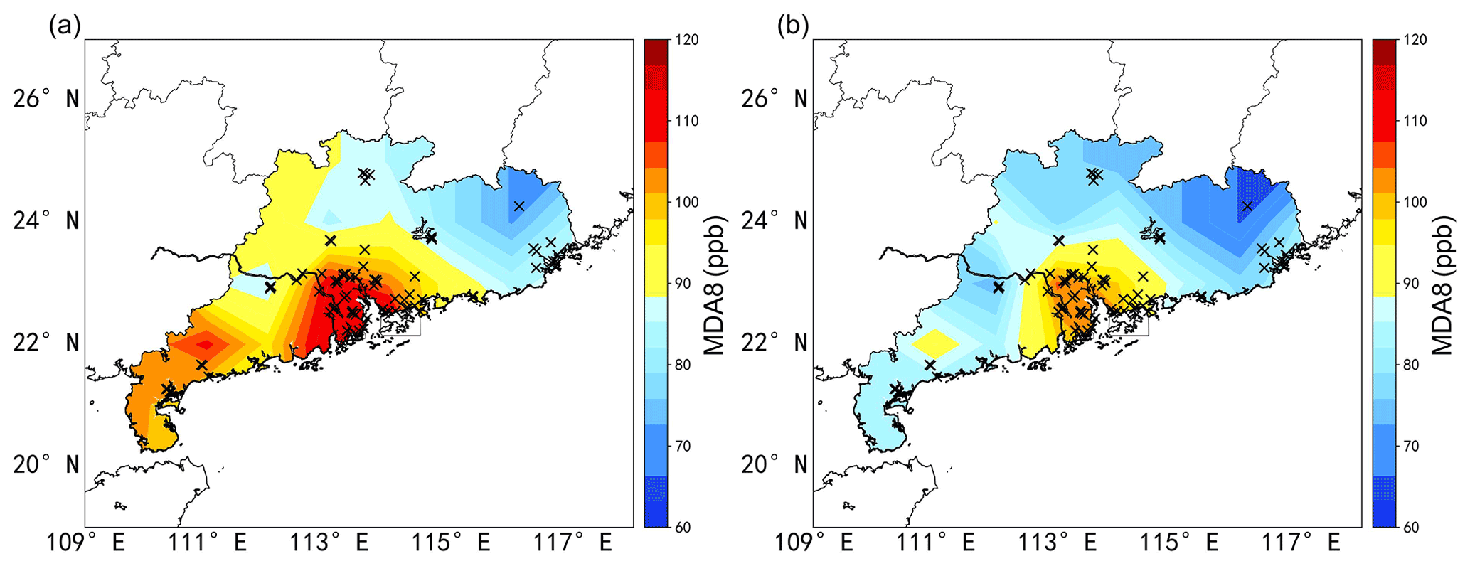
Figure 1 (a) Spatial distribution of the average maximum daily 8 h average ozone concentration (MDA8) in Guangdong during the study period, black crosses mark the locations of observation sites. (b) Same as (a) but for MDA8 of all ozone exceeding days in Guangdong in 2018 and 2019.

Hourly meteorological data are obtained from the European Centre for Medium-Range Weather Forecasts ERA5 reanalysis, including relative humidity (RH), 2 m temperature (T), 10 m zonal wind (U₁₀), 10 m meridional wind (V₁₀), geopotential height, cloud cover, surface net solar radiation, boundary layer height and K index, with a resolution of 0.25^∘ × 0.25^∘ (available at https://www.ecmwf.int/, last access: 10 November 2021).

2.2 Methods

2.2.1 Derivation of nitric oxide (NO) concentration

Since the observation of NO concentration ([NO]) is severely limited in the CNEMC data set, we calculate [NO] from the assumption of photochemical equilibrium between [NO₂] and [O₃] according to the following equation:

$$\begin{array}{}\text{(1)}& \left[\mathrm{NO}\right]={\displaystyle \frac{J_{{\mathrm{NO}}_{\mathrm{2}}}\times \left[{\mathrm{NO}}_{\mathrm{2}}\right]}{\left[{\mathrm{O}}_{\mathrm{3}}\right]\times k_{\mathrm{1}}}},\end{array}$$

where k₁ represents the reaction rate constant for the reaction of NO with O₃. This equation neglects the reactions of NO reactions with HO₂ and RO₂. The uncertainty due to this neglection is around 20 %, which is acceptable as discussed in Sect. 3.5. The value of k₁ is taken from Seinfeld and Pandis (1998):

$$\begin{array}{}\text{(2)}& k_{\mathrm{1}}\left(\mathrm{1}\mathrm{ppm}{\min }^{-\mathrm{1}}\right)=\mathrm{3.23}\times {\mathrm{10}}^{\mathrm{3}}\exp \left(-\mathrm{1430}/T\right).\end{array}$$

$J_{{\mathrm{NO}}_{\mathrm{2}}}$ is the photolysis rate of NO₂. Its value depends on the solar zenith angle (χ) and total shortwave radiation (TSR) (Wiegand and Bofinger, 2000):

$$\begin{array}{}\text{(3)}& J_{{\mathrm{NO}}_{\mathrm{2}}}=\left\{\begin{array}{ll}\mathrm{TSR}\times [\left(\mathrm{4.23}\times {\mathrm{10}}^{-\mathrm{4}}\right)& \\ +\mathrm{1.09}\times \frac{{\mathrm{10}}^{-\mathrm{4}}}{\cos \mathit{\chi }}]& \mathrm{0}{}^{\circ }\le \mathit{\chi }\le \mathrm{47}{}^{\circ },\\ & \\ \mathrm{TSR}\times \left(\mathrm{5.82}\times {\mathrm{10}}^{-\mathrm{4}}\right)& \mathrm{47}{}^{\circ }<\mathit{\chi }\le \mathrm{64}{}^{\circ },\\ & \\ \mathrm{TSR}\times [\left(-\mathrm{0.997}\times {\mathrm{10}}^{-\mathrm{4}}\right)& \\ +\left(\mathrm{1.2}\times {\mathrm{10}}^{-\mathrm{3}}\right)& \\ \times \left(\mathrm{1}-\cos \mathit{\chi }\right)]& \mathrm{64}{}^{\circ }<\mathit{\chi }\le \mathrm{90}{}^{\circ }.\end{array}\right.\end{array}$$

2.2.2 Derivation of VOC

In this study, we use CO as a tracer to estimate VOC. This tracer method has been widely used in previous studies (Heald et al., 2003; Hsu et al., 2010; Shao et al., 2011; Yao et al., 2012; Tang et al., 2013). Individual VOCs at 08:00 local time (LT) are calculated by multiplying the freshly emitted CO at 08:00 LT with the ratio of $\mathrm{VOC}/\mathrm{CO}$ in the emission inventories of Huang et al. (2021), according to the equations listed in the Supplement. The freshly emitted CO is assumed to be the difference in CO between 08:00 and 13:00 LT as shown in Fig. 2 (Eq. S1 in the Supplement). The CO at 13:00 LT is considered to be the leftover CO for the following day and is used to evaluate the leftover VOCs (Eq. S2). Oxidized VOCs (OVOCs) are estimated from the observed ratios of CH₂O, CH₃CHO and ketone to CO (Wang et al., 2016; Wu et al., 2020). Other OVOCs are not included. The VOCs and OVOCs derived this way can be validated by comparing with observed values in terms of the OH reactivity. Tan et al. (2019) reported that observed NO_x, CO, HCHO and VOCs in PRD in autumn 2014 contributed, respectively, 14 %, 10 %, 5 %–8 % and 20 %, for a total of about 50 %, to the observed OH reactivity, which scale to 28 %, 20 %, 10 %–16 % and 40 %, respectively, when normalized to 100 %. In comparison, in our study the average NO_x, CO, OVOCs and VOCs contribute 33 %, 17 %, 24 % and 26 %, respectively, to the OH reactivity. There is a reasonable agreement between our results and those of Tan et al. (2019) except for OVOCs and VOCs. The disagreement on OVOCs can be easily explained by the fact that HCHO accounts for about two-thirds of the OVOCs in our case. Nevertheless, the underestimate of the VOC contribution in our study remains unresolved and suggests significant uncertainty in the VOCs derived by our method.

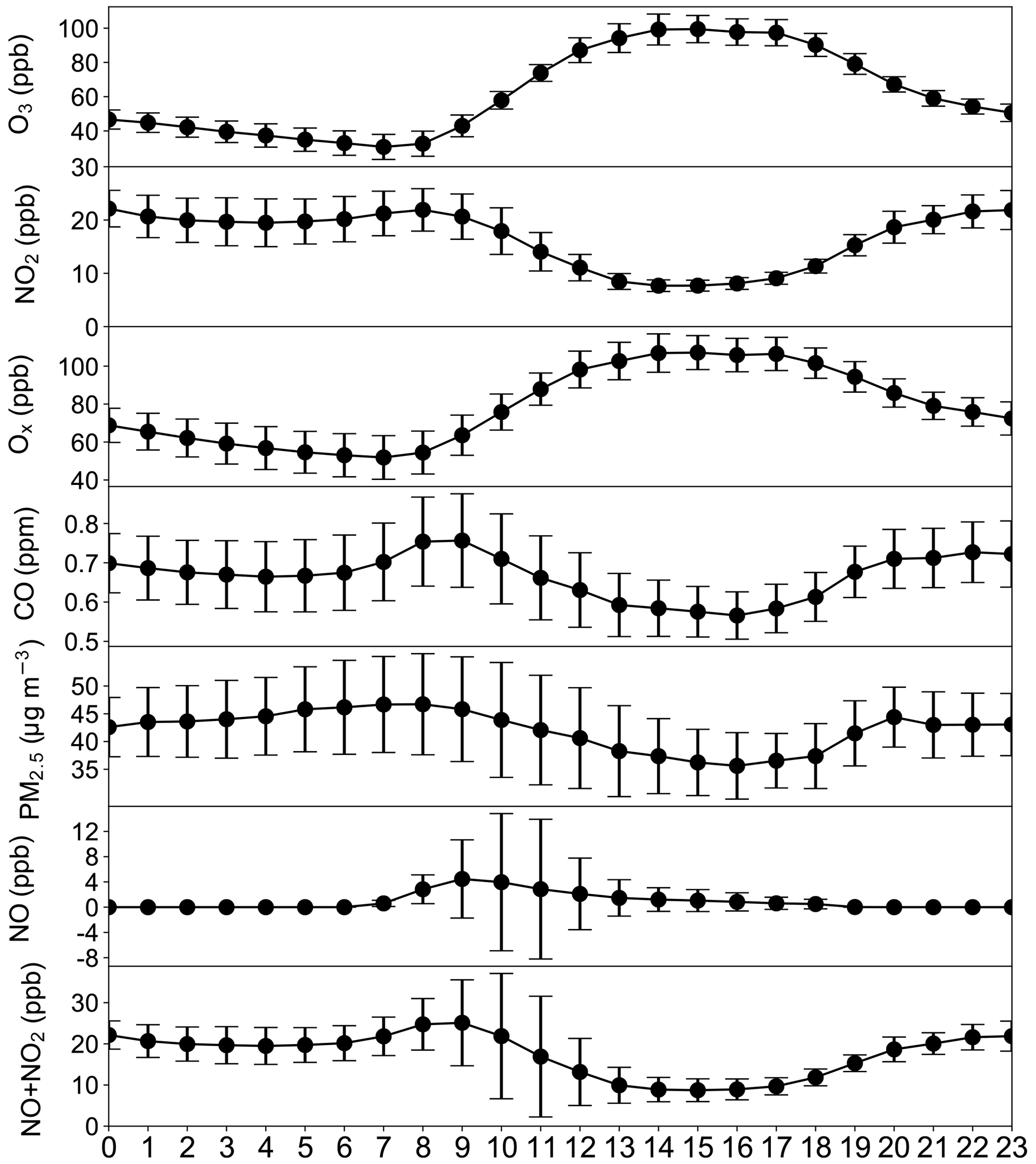
Figure 2 Average diurnal variations of air pollutants O₃, NO₂, O_x, CO, PM_2.5, NO and NO + NO₂ observed at the 77 stations in Guangdong during the two episodes.

2.2.3 Derivation of OH concentrations

The ratio ethylbenzene $/$ m,p-xylene has been suggested to be a good measure of the photochemical processing by OH (Calvert, 1976; Singh, 1977; Shiu et al., 2007). Following a Lagrangian trajectory, the ratio can be shown as

$$\begin{array}{}\text{(4)}& E/X=\left(E_{\mathrm{0}}/X_{\mathrm{0}}\right)\exp \left(-\underset{\mathrm{0}}{\overset{t}{\int }}\left(k_e-k_x\right)\left[\mathrm{OH}\right]\mathrm{d}t\right),\end{array}$$

where E and X represent concentrations of ethylbenzene and m,p-xylene at time t, respectively. E₀ and X₀ are their corresponding initial concentrations, k_x and k_e are their reaction rate constants with OH, and k_x and k_e equal to $\mathrm{2.17}\times {\mathrm{10}}^{-\mathrm{11}}$ and $\mathrm{7.0}\times {\mathrm{10}}^{-\mathrm{12}}$ cm³ s⁻¹, respectively (Atkinson, 1990). With a known value of $E_{\mathrm{0}}/X_{\mathrm{0}}$, [OH × t] can be evaluated from observed $E/X$ at time t. This provides an OBM-derived density of OH.

In the real atmosphere, the Lagrangian condition rarely exists due to turbulence mixing as well as atmospheric advection. Nevertheless, Eq. (4) tends to hold because atmospheric transport affects the two species similarly. This is a key advantage of the OBM. In this study, due to limited measurements of VOC, we use CO and NO_x to replace ethylbenzene and m,p-xylene, respectively.

2.2.4 Calculation of oxidized VOC and NO_x

In this study, we consider the reaction of NO₂ with OH as the only removal process for NO_x and assume the removal of NO_x is pseudo-first order as shown below. In this case, following the Lagrangian trajectory, we have the following:

$$\begin{array}{}\text{(5)}& \left[{\mathrm{NO}}_x\right]={\left[{\mathrm{NO}}_x\right]}_{\mathrm{0}}\exp \left(-k\underset{\mathrm{0}}{\overset{t}{\int }}\left[\mathrm{OH}\right]\mathrm{d}t\right),\end{array}$$

where k is the reaction rate constant of NO_x with OH. The reaction rate constant for NO₂ and OH is $\mathrm{1.04}\times {\mathrm{10}}^{-\mathrm{11}}$ cm³ s⁻¹ at 25 ^∘C and 1 atm pressure according to Sander et al. (2003). Since NO₂ is part of NO_x, the value of k should be scaled down by the ratio ${\mathrm{NO}}_{\mathrm{2}}/{\mathrm{NO}}_x$. The average of the ${\mathrm{NO}}_{\mathrm{2}}/{\mathrm{NO}}_x$ ratio is about 0.6, thus k for NO_x is prescribed at $\mathrm{6.0}\times {\mathrm{10}}^{-\mathrm{12}}$ cm³ s⁻¹.

Similarly, we have the following:

$$\begin{array}{}\text{(6)}& {\displaystyle }\left[{\mathrm{VOC}}_{\mathrm{s}}\right]={\left[{\mathrm{VOC}}_{\mathrm{s}}\right]}_{\mathrm{0}}\exp \left(-k_{{\mathrm{VOC}}_{\mathrm{s}}}\underset{\mathrm{0}}{\overset{t}{\int }}\left[\mathrm{OH}\right]\mathrm{d}t\right),\text{(7)}& {\displaystyle }\left[\mathrm{CO}\right]={\left[\mathrm{CO}\right]}_{\mathrm{0}}\exp \left(-k_{\mathrm{co}}\underset{\mathrm{0}}{\overset{t}{\int }}\left[\mathrm{OH}\right]\mathrm{d}t\right),\end{array}$$

where k_VOC and k_co are the reaction rate constants of VOCs and CO with OH, respectively. K_VOC values of individual VOCs are listed in Table S1 in the Supplement, and k_co is prescribed at $\mathrm{1.4}\times {\mathrm{10}}^{-\mathrm{13}}$ cm³ s⁻¹ (Atkinson et al., 2006).

Since the Lagrangian condition is sometimes not observed, it is necessary to select the time periods during which the quasi-Lagrangian condition as shown in Fig. 2 is approximately valid. The selection criterion is that the ratio of CO concentrations between 08:00 and 13:00 LT lies within 50 % of 1 standard deviation (vertical bars) of the ratio of CO shown in Fig. 2, which is assumed to be in the Lagrangian condition. This criterion usually filters out about 60 % of data; i.e., about 40 % of the days satisfy approximately the Lagrangian condition. We have tested this selection criterion by parameterizing it between 30 % and 80 % of 1 standard deviation and found our major results are robust within this range.

2.2.5 Dilution effect

Diurnal variations of pollutants averaged over all stations and the two episodes are shown in Fig. 2. Previous studies have shown that part of the early-morning rise in O₃ is due to O₃ entrained from the residual layer above the boundary layer during the development of the boundary layer in the morning (Shiu et al., 2007; Zhao et al., 2019). We adopt the approach proposed by Shiu et al. (2007) to account for the dilution effects. Specifically, the reduction of CO concentrations from 08:00 to 13:00 LT (approximately 20 %) is assumed to be the dilution effect and used for all other species. The uncertainty due to this assumption is discussed in Sect. 3.5.

2.2.6 Emissions of NO_x, CO and VOCs between 08:00 and 13:00 LT

Equations (5), (6) and (7) do not account for the emissions of NO_x, CO or VOC during the period of 08:00–13:00 LT. Inclusion of these emissions would affect the value of OH derived from Eq. (5) as well as the dilution effect. We estimate the emission of NO_x by taking advantage of the fact that NO_x reaches a quasi-steady state around 13:00–16:00 LT as evident in Fig. 2. We believe that the quasi-steady state is maintained by the balance between the oxidation of NO_x and its emission. This is based on the notion that oxidation of NO₂ by OH is the predominant sink of NO_x in 13:00–16:00 LT, of which the integration over the mixed or boundary layer should be balanced by the emission flux of NO_x according to the continuous equation of NO_x. Assuming the oxidation loss rate of NO_x in the mixed layer is uniform with height, we obtain that the divergence of the hourly NO_x emission rate is equal to the oxidation loss rate of NO_x at 13:00–16:00 LT. Using the average OH of 5×10⁶ cm⁻³ at noon derived from Eq. (5) (Fig. 4) and mean NO_x at 13:00–16:00 LT (Fig. 2), a value of approximately 1.8 ppb h⁻¹ can be obtained. This value is assumed to be the hourly NO_x emission rate between 08:00 and 13:00 LT. The emissions of CO and VOC are calculated using their ratios to NO_x in the emission inventories of Huang et al. (2021).

2.2.7 Box model

A photochemical box model with a carbon bond mechanism (PBM-CB05) (Yarwood et al., 2005; Coates and Butler, 2015; Y. Wang et al., 2017) is used to simulate the O₃ production rate and OH radical. Unlike emission-based models, the PBM-CB05 used in this study is based on observed concentrations of air pollutants and meteorological parameters (Y. Wang et al., 2017). In the CB05 module, VOCs are grouped according to carbon bond type and the reactions of individual VOCs are condensed using the lumped structure technique (Yarwood et al., 2005; Coates and Butler, 2015). In this study, the pollution indicators (O₃, NO, NO₂, CO and VOC) and meteorological parameters (temperature, relative humidity, pressure) observed during the two episodes are utilized as input parameters for the model. There are 37 VOC species considered in our case. The model simulation starts from 07:00 and ends at 18:00 LT with hourly input data based on observed concentrations of air pollutants and meteorological parameters during the two episodes.

3 Results and discussion

3.1 Air quality and meteorological conditions

Figure 3 shows the time series of hourly concentrations of air pollutants. The time period covers the two ozone episodes and extends to 2 d before and 2 d after. Mean maximum daily 8 h average (MDA8) O₃ concentrations in episode 1 was 88.7 ppb, and in episode 2 was 99.6 ppb. The average daily concentration of CO of the two episodes was 0.74 and 0.85 ppm, respectively. The corresponding time series of key meteorological parameters are shown in Fig. S1 in the Supplement. As O₃ is formed through photochemical reactions involving precursors NO_x and VOC, strong solar radiation, high temperature and low wind speed have been identified to be common conditions conducive to the formation of ozone (Liu et al., 2017; L. Wang et al., 2018). During both O₃ episodes, the weather in Guangdong was dominated by high-pressure systems with warm and cloudless conditions, and northeasterly winds. In particular, the average maximum temperature for episode 1 was 28^∘ and for episode 2 was 30^∘.

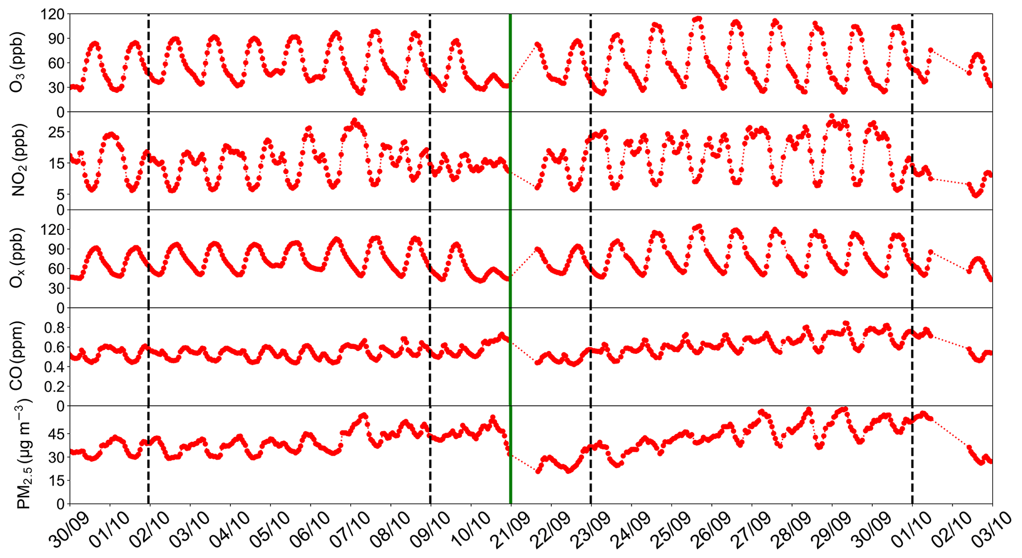
Figure 3 Hourly surface concentrations of air pollutants during the study period. The green line is added to separate the two episodes; the black dashed lines indicate 2 d before and 2 d after the episodes.

The general patterns of O₃ concentrations of the two episodes were similar. Relatively high O₃ concentrations with northerly or northeasterly winds appeared at least 2 d before the episode in both episodes. Afterward, the high O₃ kept increasing or stayed at a high level until the prevailing northeasterly wind shifted away and the surface pressure dropped. Starting on 22 September 2018, a precipitation event occurred which obviously ended the first episode. The heavier cloud cover greatly reduced the intensity of solar radiation and O₃ photochemical formation reactions. The disappearance of high O₃ in the second episode is believed to be related to a shift to southerly winds that brought in clean moist air from the South China Sea.

3.2 OH concentrations derived from OBM

Figure 4 shows the hourly OH concentrations between 08:00 and 13:00 LT derived from Eq. (4) based on the concentrations of NO_x and CO observed at the 77 stations. Average OH concentrations derived at the 77 stations between 08:00 and 13:00 LT stay within a narrow range of 2.5×10⁶ cm⁻³ to 5.5×10⁶ cm⁻³ with a weak dependence on the NO_x. The mean OH concentrations and their 1 standard deviations derived by the OBM (black dots and black vertical bars, respectively) are approximately 30 % higher than the mean OH concentrations and 1 standard deviations observed at a rural station in PRD in October–November 2014 (blue line and blue shade, respectively) (Tan et al., 2019). Nevertheless, there is a complete overlap of the 1 standard deviations of the two data sets (blue shade and black vertical bars), which indicates a good agreement between our OBM OH values and those observed by Tan et al. (2019). In another comparison with a previous investigation, our OH concentrations are approximately 40 % lower than the OH calculated by a box model constrained by observed air pollutants during an experiment at a remote island site in the PRD from August to November 2013 (red line and red shade) (Y. Wang et al., 2018). There is also a nearly complete overlap of the 1 standard deviations of the two data sets (red shade and black vertical bars). Figure 4 also includes the noon OH concentrations calculated by the box model described above. The box model is constrained by the ambient conditions observed during the two episodes. The average modeled OH concentration is approximately 3.2×10⁶ cm⁻³ with a 1 standard deviation of 0.6×10⁶ cm⁻³ (red cross and red vertical bar, respectively). This value of OH is approximately 40 % less than the OH values of $\mathrm{5.5}\pm \mathrm{4.3}\times {\mathrm{10}}^{\mathrm{6}}$ cm⁻³ derived by the OBM at noon. Again, there is a good overlap of the 1 standard deviations of the two data sets. The agreement among the OH concentrations derived by the OBM, the box model and field observations gives credence to our observation-based analysis, at least in terms of the derived OH concentration which plays a critical role in the O₃ formation.

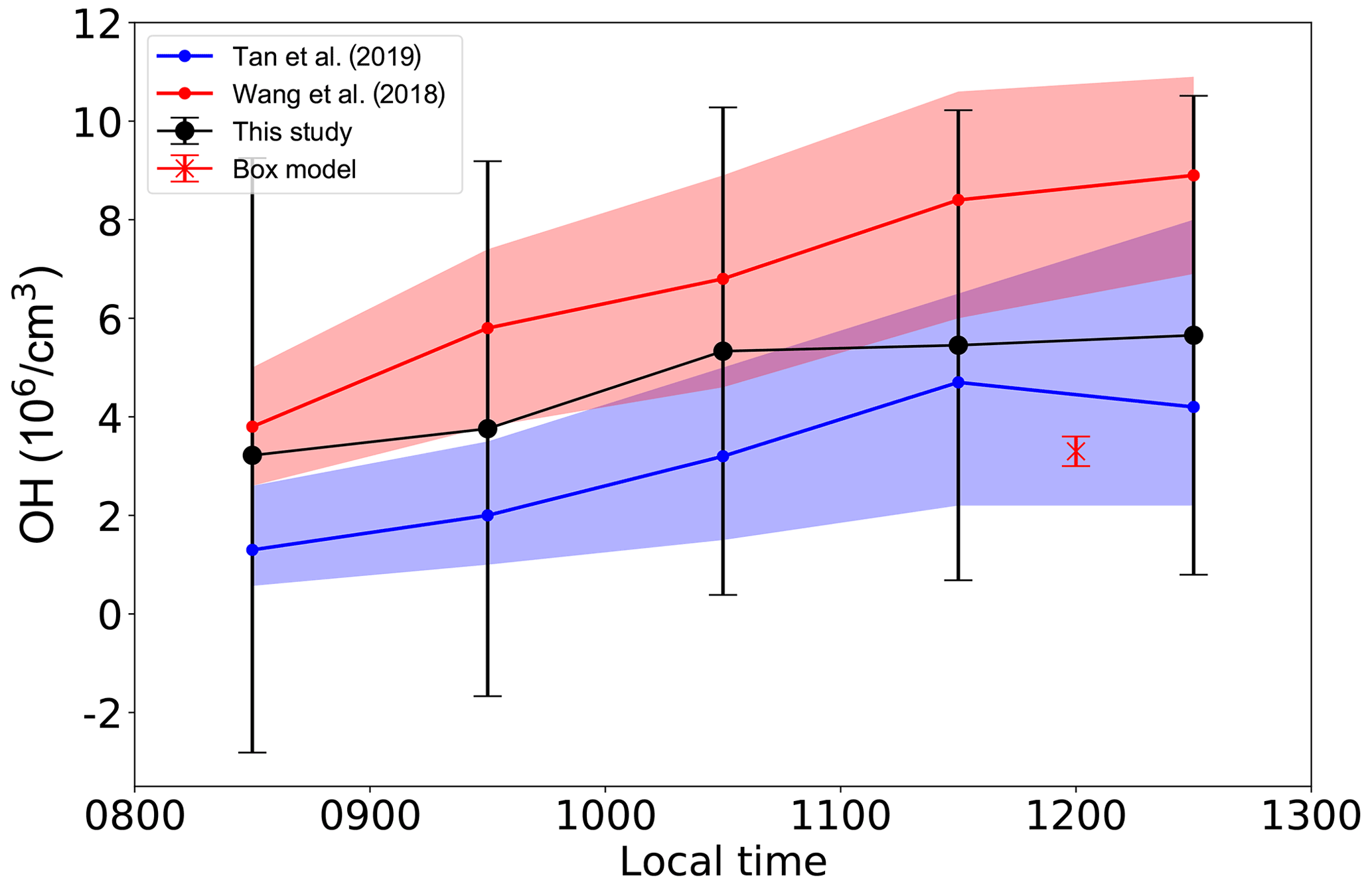
Figure 4 Hourly average OH concentrations between 08:00 and 13:00 LT derived from the OBM are shown in the black line with black dots; observed OH concentrations by Tan et al. (2019) are shown in the blue line and blue shade; calculated OH concentrations by Y. Wang et al. (2018) are shown in the red line and red shade. The blue shade denotes the 25 % and 75 % percentiles of the data; the red shade indicates the 95 % confidence interval of the data. The red cross with red vertical whiskers denotes the mean OH concentration and 1 standard deviation, respectively, calculated by a box model constrained by observed ambient conditions during the two episodes.

Nevertheless, we acknowledge that the OH concentrations derived here are approximately a factor of 3 to 5 lower than the OH concentrations observed at Backgarden (a suburban site about 70 km downwind of Guangzhou) during an intensive campaign in 2006, in which the OH reached daily peak values of 15–26 × 10⁶ cm⁻³ (Lu et al., 2012). This discrepancy remains unresolved.

3.3 Ozone production efficiency

Ozone production efficiency (ε) is defined as the number of O₃ molecules produced per molecule of NO_x (or VOC) oxidized photochemically (Liu et al., 1987; Trainer et al., 2000). ε can be calculated by the following equations:

$$\begin{array}{}\text{(8)}& {\displaystyle }\mathit{\epsilon }\left[{\mathrm{NO}}_x\right]=\mathrm{\Delta }\left[{\mathrm{O}}_{\mathrm{3}}\right]/\mathrm{\Delta }\left[{\mathrm{NO}}_x\right],\text{(9)}& {\displaystyle }\mathit{\epsilon }\left[\mathrm{VOC}\right]=\mathrm{\Delta }\left[{\mathrm{O}}_{\mathrm{3}}\right]/\mathrm{\Delta }\left[\mathrm{VOC}\right],\end{array}$$

where Δ[O₃] represents the amount of ozone generated from 08:00 to 13:00 LT which is equal to the observed difference in O₃ between 08:00 and 13:00 LT, after adjustment to the dilution factor. Δ[NO_x] (Δ[VOC]) represents the consumption and oxidation of NO_x (VOC) between 08:00 and 13:00 LT.

Figure 5a shows the relationship of ε as a function of the average NO_x concentration between 08:00 and 13:00 LT. As expected ε is greater at lower NO_x; i.e., the O₃ production efficiency is greater in rural and suburban environments than urban conditions, in agreement with previous findings (Liu et al., 1987; Kleinman et al., 2002). The value of ε(NO_x) converges to a narrow range of about 1.0±0.5 when NO_x is greater than 70 ppb. This range of ε(NO_x) in Fig. 5a is consistent with previous investigations in urban environments (Sillman et al., 1998; Daum et al., 2000) as well as in rural environments (Chin et al., 1994; Trainer et al., 1995). Compared to previous investigations in PRD areas, values in Fig. 5a at NO_x higher than 20 ppb are in good agreement with the ε(NO_x) values of 2.1–2.5 found at urban stations in PRD by Yu et al. (2020) and Lu et al. (2010b). However, ε(NO_x) values of 6.0–13.3 were found at rural stations in PRD (Lu et al., 2010b; Wei et al., 2012; Xu et al., 2015; Yang et al., 2017), which are about a factor of 2 higher than our values at low NO_x. Considering that our values are derived for two ozone pollution episodes in which the ε(NO_x) should be higher than non-episode periods, this discrepancy is puzzling. Figure 5b is the same as Fig. 5a except that the x axis is changed to Δ[NO_x] or the oxidized NO_x. Figure 5b shows a relatively smoother distribution compared to Fig. 5a, most likely because the oxidized NO_x, rather than NO_x itself, is more closely related photochemically to Δ[O₃]. As Δ[NO_x] increases beyond 30 ppb, ε[NO_x] levels off linearly to a nearly constant value around 1.0 when Δ[NO_x] approaches 80 ppb (Fig. 5b). ε[VOC] is also greater at lower Δ[VOC] and has an asymptotic value of about 1.0±0.5 when Δ[VOC] becomes greater than 50 ppb (Fig. 5c).

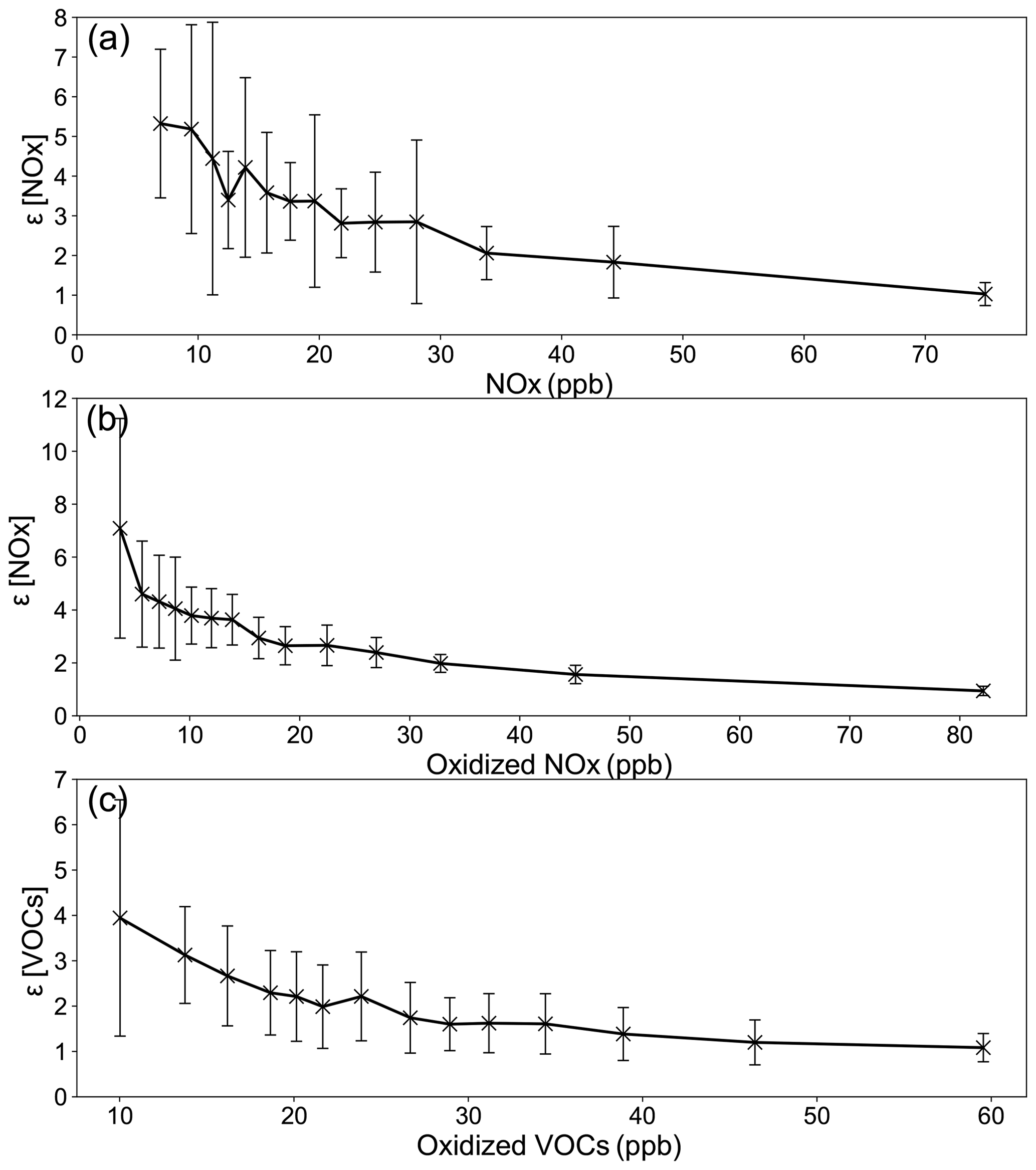
Figure 5 Ozone production efficiency plotted as a function of NO_x (a), oxidized NO_x (b) and oxidized VOC (c).

Figure 5b and c have some useful implications for the ozone control strategy. For instance, ε[NO_x]=1.7 when Δ[NO_x]=50 ppb can be interpreted as in a highly polluted ambient environment in Guangdong where Δ[NO_x] equals 50 ppb, approximately 1.7 ppb of ozone is produced for each ppb of NO_x oxidized. The overall average value of ε[NO_x] is about 3.0 (Fig. 5b), which implies on average 3.0 ozone molecules are produced for each NO_x molecule oxidized. The overall average value of ε[VOC] is approximately 2.1 (Fig. 5c), which implies 2.1 ozone molecules are produced for each VOC molecule oxidized, which is about 50 % less efficient than that of NO_x.

Photochemical oxidation of a VOC molecule under common ambient urban conditions produces approximately two or more peroxyl radicals – one HO₂ and more than one RO₂ (Seinfeld and Pandis, 1998; Jacob, 1999). Because there is abundant NO_x in the ambient atmosphere in Guangdong, nearly all peroxyl radicals are expected to react with NO to produce NO₂ and then O₃. Jacob (1999) suggested an ozone formation rate of 2Δ[VOC] in the urban atmosphere. This is in excellent agreement with the overall value of 2.1Δ[VOC] found here by the OBM. This agreement, as well as the consistency with previous investigations on the ε[NO_x], provides credence again to the observation-based analysis of this study.

3.4 Ozone sensitivity to precursors

The sensitivity of ozone formation (ΔO₃) to ozone precursor NO_x is examined in Fig. 6a, in which ΔO₃ (right-hand side in red) and the oxidized VOC (left-hand side in black) are plotted as a function of the oxidized NO_x. Similarly in Fig. 6b ΔO₃ (right-hand side in red) and the oxidized NO_x (left-hand side in black) are plotted as a function of the oxidized VOC. It can be seen in Fig. 6a that ΔO₃ increases with the value of oxidized NO_x. The increase first has a very sharp slope of about 2.0 ppb ppb⁻¹ when oxidized NO_x is below 30 ppb, indicating a strong sensitivity of ozone formation to oxidized NO_x. The slope flattens out quickly to around 0.2 ppb ppb⁻¹ when oxidized NO_x gets greater than 30 ppb, suggesting other factors such as VOC and the $\mathrm{VOC}/{\mathrm{NO}}_x$ ratio may become more important in controlling the ozone formation rate. Figure 6b shows that ΔO₃ increases with the value of oxidized VOC with a slope of about 0.4 ppb ppb⁻¹. However, this slope is much smaller than that of NO_x, especially in the low oxidized NO_x regime (<30 ppb). In a brief summary for Fig. 6a and b, the ozone formation is most sensitive to the oxidized NO_x in relatively clean regimes of oxidized NO_x < 30 ppb. In more polluted regimes, other factors such as the initial VOC and/or the $\mathrm{VOC}/{\mathrm{NO}}_x$ ratio appear to have a significant impact on the ozone formation. Additional evidence in support of these points is elaborated below.

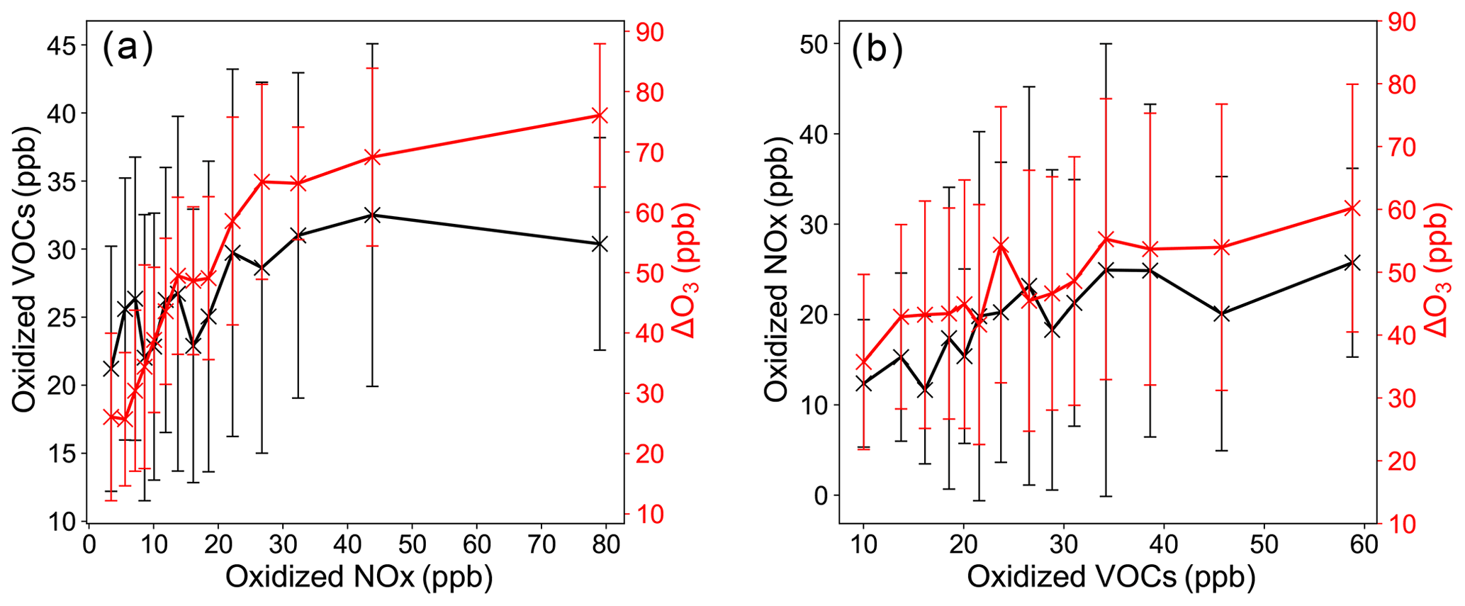
Figure 6 Ozone formation rate (ΔO₃, right-hand side in red) and the oxidized VOC (left-hand side in black) plotted as a function of oxidized NO_x (a). Ozone formation rate (ΔO₃, right-hand side in red) and oxidized NO_x (left-hand side in black) plotted as a function of the oxidized VOC (b).

Figure S2 presents a three-dimensional EKMA-like depiction of ozone formation rates (ΔO₃, black dots, 471 points) plotted as a function of the oxidized NO_x (x axis) and oxidized (VOCs + CO) (y axis). The colored plane is a linear regression to the ozone formation rates (black dots), and the green and red bars denote positive and negative deviations of individual dots from the plane, respectively. Different color shades from blue to red denote different concentrations of ΔO₃ in ppb. The equation for [ΔO₃] represents the plane as a function of the oxidized NO_x (ΔNO_x) and oxidized VOC (ΔVOC). The coefficients in front of ΔNO_x and ΔVOC in the equation are the ozone sensitivities to ΔNO_x and ΔVOC, respectively. The plane fits the black dots (ozone formation rates) reasonably well with an R² value of 0.423. The coefficient of ΔNO_x is 0.755 which is about 3 times of that of ΔVOC (0.247), indicating the ozone formation rate is about 3 times more sensitive to ΔNO_x than ΔVOC when considering all data at the 77 stations in Guangdong during the two episodes. This is consistent with the findings from Fig. 6a and b.

Some uneven congregations of red and green bars appear; e.g., a large number of red bars have low values of ΔNO_x, while many green bars tend to have moderate values of ΔNO_x and high values of ΔVOC. This suggests that there is a need to divide Fig. S2 into different congregations or regimes. Figure 7 is the same as Fig. S2 except it is divided into four quadrants of different levels of oxidized ozone precursors: panel (a) shows low ΔNO_x and low ΔVOC (ΔNO_x<20 ppb, ΔVOC<25 ppb), panel (b) shows high ΔNO_x and high ΔVOC (ΔNO_x>20 ppb, ΔVOC>25 ppb), panel (c) shows low ΔNO_x and high ΔVOC (ΔNO_x<20 ppb, ΔVOC>25 ppb), panel (d) shows high ΔNO_x and low ΔVOC (ΔNO_x>20 ppb, ΔVOC<25 ppb).

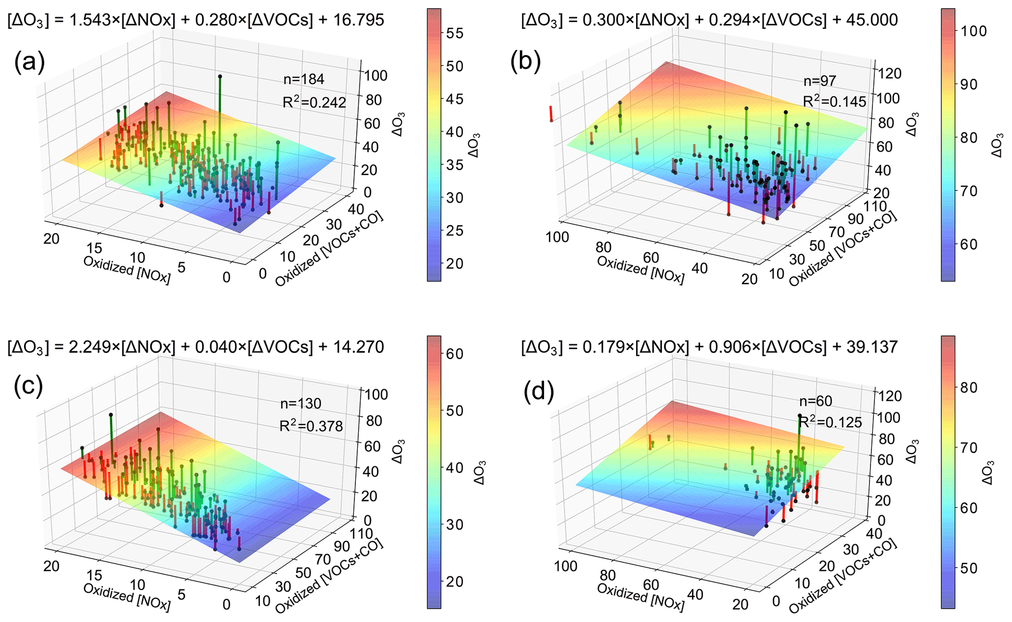
Figure 7 Three-dimensional depiction of ozone formation rate (ΔO₃, z axis) plotted as a function of oxidized NO_x (x axis) and oxidized VOC (y axis). The black dots denote values of ΔO₃, the colored plane is the best linear fit to the black dots, and the green and red bars denote positive and negative deviations from the plane, respectively. The equation listed represents the surface as a function of oxidized NO_x and oxidized VOC. R² is the square of correlation coefficient of the linear regression. Four quadrants: (a) low NO_x and low VOC (NO_x < 20 ppb, VOC < 25 ppb), (b) high NO_x and high VOC (NO_x > 20 ppb, VOC > 25 ppb), (c) low NO_x and high VOC (NO_x < 20 ppb, VOC > 25 ppb), (d) high NO_x and low VOC (NO_x > 20 ppb, VOC < 25 ppb).

In total, 39 % of all data points (184 out of 471 points) lie in panel (a), the slope of ΔO₃ against ΔNO_x (coefficient of ΔNO_x in the equation) is approximately 1.54 ppb ppb⁻¹ (p value < 0.01), while the slope of ΔO₃ against ΔVOC (coefficient of ΔVOC) has a value of 0.28 ppb ppb⁻¹ (p value = 0.021). These values of slopes imply that the ozone formation at stations in panel (a), a relatively clean environment, is about 5 times more sensitive to ΔNO_x than ΔVOC; i.e., the ozone formation is NO_x-limited. This is in good agreement with the conclusion reached based on Figs. 6a, b and S2. Panel (b) contains about 20 % of the data points. The coefficient of ΔNO_x is 0.3 ppb ppb⁻¹ (p value < 0.01), while the coefficient of ΔVOC is 0.29 ppb ppb⁻¹ (p value = 0.043), suggesting that the ozone formation is sensitive to both ΔVOC and ΔNO_x. This quadrant belongs to the transitional regime. Panel (c) has 28 % of the data points, and the coefficients of ΔNO_x and ΔVOC are 2.25 ppb ppb⁻¹ (p value < 0.01) and 0.04 ppb ppb⁻¹ (p value = 0.785), respectively. Here again the ozone formation is NO_x-limited. Panel (d) has 13 % of the data points, the coefficients of ΔNO_x and ΔVOC are 0.18 ppb ppb⁻¹ (p value = 0.126) and 0.91 ppb ppb⁻¹ (p value = 0.037), respectively. These values of coefficients indicate that the ozone formation is more sensitive to ΔVOC than ΔNO_x; i.e., the ozone formation is VOC-limited.

The analysis above provides an observation-based method for evaluating the ozone-precursor sensitivity. This method has the potential to provide quantitative information on the ozone control strategy for individual regions. In theory, the quadrants can be further divided into, for example, a specific region represented by individual stations, such that an ozone control strategy suitable to the region could be developed. In practice, this is limited by the data available for making the three-dimensional plot like Fig. 7.

We have compared the OBM results to those of the box model constrained by the observed ambient environment in this study. Figure 8 shows the traditional 2D-EKMA plot calculated by the model. To facilitate the comparison, the x axis and y axis in Fig. 8 are changed to hourly oxidized NO_x and oxidized VOC, respectively, rather than the usual early-morning concentrations of NO_x and VOC. The modeled results are shown in colored isopleths of ozone increments between 06:00 and 16:00 LT, while results of the OBM are shown in colored dots for ozone increment or formation between 08:00 and 13:00 LT. The difference in the length of time has a negligible effect on the ozone increment as evident in Fig. 2. The OBM values agree with the model results semi-quantitatively. For instance, the colored dots of OBM shift from blue (20 ppb) to green (60–80 ppb) consistently with the colored isopleths, but the OBM dots rarely turn yellow when modeled isopleths become greater than 90 ppb. Two red lines (left red and right red) are added to Fig. 8 to facilitate the assessment of the sensitivity of ozone formation. There are 127 points located to the left of left red line, which clearly belongs to the NO_x-limited regime according to the modeled ozone isopleths. There are 141 points located to the right of right red line, which clearly belongs to the VOC-limited regime according to the modeled ozone isopleths. In between the two red lines there are 203 points, which are in the transitional regime sensitive to both NO_x and VOC. These three regimes overlap and agree in ozone formation sensitivity with panels (a) and (c), panel (d) and panel (b) of the OBM results, respectively. However, the numbers of points in the three regimes deviate significantly from those of the four OBM quadrants. For example, panel (b) has only 97 points compared to the 203 points in the transitional regime of Fig. 8; panel (d) has only 60 points compared to the 141 points in the VOC-limited regime of Fig. 8; while panels (a) and (c) have 314 points compared to the 127 points in an NO_x-limited regime of Fig. 8. In terms of ozone sensitivity, the modeled results show a nearly equal number of points in the NO_x-limited regime as the VOC-limited regime, while the OBM results show five to one in favor of the NO_x-limited regime. A quantitative agreement between the OBM results (dots) and the modeling results (isopleths) would require shifting the dots in Fig. 8 leftward by approximately 0.5–1 ppbv h⁻¹, which would mean a reduction of OH by approximately 30 %–50 %. Interestingly this requirement matches well with the fact that modeled OH is approximately 40 % less than the OH value derived by the OBM at noon as shown in Fig. 4.

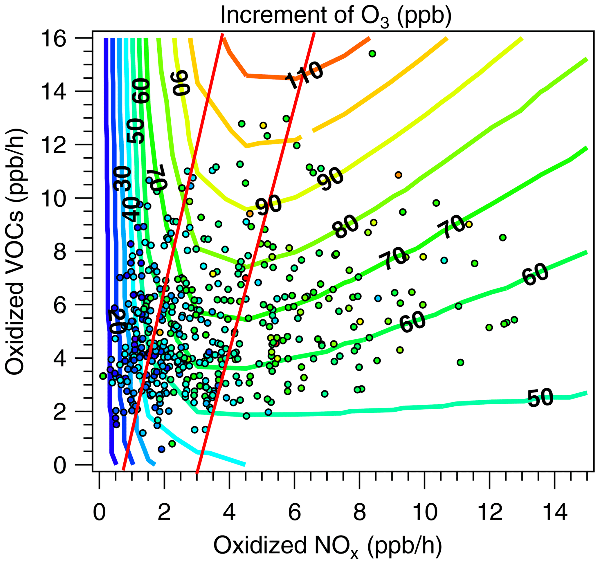
Figure 8 Ozone isopleths (in ppbv) of traditional 2D-EKMA plot for the two episodes calculated by the box model are shown in colored lines, ozone concentrations at 13:00 LT derived by the OBM are shown in colored dots, and the x axis and y axis are hourly oxidized NO_x and oxidized VOC, respectively.

Comparing with previous studies, we notice that almost all previous researches suggested that limiting the emission of VOCs in Guangdong would have a positive role in reducing ozone reduction (Zhang et al., 2008; T. Wang et al., 2017; Jiang et al., 2018), but different results may appear in different places and time. Yu et al. (2020) found that NO_x reduction in Shenzhen has led to higher ozone production from 2015 to 2018 given the nearly constant VOCs. However, the ozone mitigation would be benefit from further NO_x reduction under the conditions of 2018. Yang et al. (2019) analyzed the relationship between ozone and precursors in PRD from 2007 to 2017 and found that the northeastern PRD was NO_x-limited and the southwest VOC-limited. Obviously, these findings are in general different from our results except in a highly polluted environment like panel (b). Some of the difference can be explained by the fact that most of the previous studies were focused on urban regions, while many rural stations are included in our OBM analysis. Finally, we acknowledge that our results are based on the analysis of only two multi-day ozone episodes which maybe not representative of the general ambient environment in Guangdong. A comprehensive regional and temporal OBM analysis is needed to make a definitive comparison with previous findings.

In summary of Sect. 3.4, the sensitivity of ozone formation to its precursors is complex and highly dependent on the ambient conditions of the station day. Our OBM shows that approximately 67 % of the station days exhibit ozone formation sensitivity to NO_x, approximately 20 % of the station days are in the transitional regime sensitive to both NO_x and VOC; only approximately 13 % of the station days are sensitive to VOC. These findings are different from results of most previous studies, which favor ozone formation sensitivity to VOC.

3.5 Uncertainty analysis

Significant uncertainties and limitations exist in our OBM analysis. First and foremost is the uncertainty involved with the Lagrangian air mass assumption, which does not take into account mixing, entrainment or surface deposition effects. Omitting the mixing of NO_x emitted between 08:00 and 13:00 LT into the Lagrangian air mass can lead to an underestimate of the OH concentration, while omitting the mixing of CO emission can underestimate the dilution effect. We account for the mixing of NO_x emission by assuming that NO_x reached a quasi-steady state around 13:00–16:00 LT (Sect. 2.2.6), and in turn the mixing of CO and VOC emissions are calculated using their ratios to NO_x in the emission inventories of Huang et al. (2021). However, no surface deposition effect is included. The selection criterion defined by 50 % of 1 standard deviation (1.0±0.5σ) from the mean CO distribution works well in filtering out those data deviating significantly from the Lagrangian condition. However, the criterion filters out about 60 % of the data, thus limiting the representativeness of the OBM analysis. This limitation has been evaluated by relaxing the selection criterion to 1.0±0.8σ, which filters out only about 30 % of the data. No significant difference has been detected, suggesting the results of the OBM analysis are representative of the majority of the data. Another source of uncertainty is that one single dilution factor is adopted for all air pollutants, including O₃, CO, PM_2.5 and NO_x. In this context, it is reassuring to find out that the dilution factors derived independently from CO and PM_2.5 agree within 10 % with each other. In a brief summary, we estimate the uncertainty involved with the Lagrangian assumption to be in the range of 20 %–40 %.

The second largest source of uncertainty is the evaluation of VOCs. Individual VOCs, including OVOCs, are calculated based on the observed concentration of CO and the ratio of $\mathrm{VOC}/\mathrm{CO}$ in the emission inventories as discussed in Sect. 2.2.2. We have evaluated the VOCs and OVOCs derived this way by comparing their contributions to the OH reactivity observed by Tan et al. (2019) in PRD in autumn 2014. There is a reasonable agreement between our estimates of the contributions of NO_x, CO, OVOCs and VOCs to the OH reactivity and those of Tan et al. (2019) except for a 35 % underestimation of VOCs. Hence we estimate the uncertainty in the evaluation of VOCs to be in the range of 30 %–50 %.

Another source of uncertainty may come from the neglection of heterogeneous reactions in this study. The largest impact of neglecting heterogeneous reactions is most likely to involve NO_x between 08:00 and 13:00 LT, during which the OH is derived. Since the effect of heterogeneous reactions is included in the observations, the neglection of any heterogeneous removal of NO_x (e.g., deposition of NO_x on aerosols in the humid conditions in Guangdong) can lead to an overestimate of OH concentrations by the OBM. This would have a significant impact on the outcome of this study, as OH plays a critical role in the photochemistry of NO_x, VOCs and ozone. On the other hand, presence of significant natural sources of NO_x such as biogenic emission and/or lightning source in 08:00–13:00 LT would lead to an underestimate of OH concentration.

Finally, another source of uncertainty is attributable to the coarse resolution of CO measurements which is reported at 0.1 ppm intervals. As a result, many hourly CO data would show identical values and lose their value as a tracer.

4 Summary and conclusions

In this study, two persistent elevated ozone episodes in Guangdong (77 stations) that occurred on 2–8 October 2018 and 24 September–1 October 2019 were analyzed to investigate the sensitivity of ozone generation to precursor concentrations at the 77 stations. An OBM is developed by modifying the approach suggested by Shiu et al. (2007). Specifically, NO_x and CO are used in this OBM to substitute for the two hydrocarbon species utilized in Shiu et al. (2007).

Major outputs from the OBM include the OH concentrations, O₃ production efficiency and the sensitivity of ozone formation to the precursors at the 77 stations during the two ozone episodes. The average OH concentrations between 08:00 and 13:00 LT agree well with the OH values observed at a rural station in PRD in October–November 2014 by Tan et al. (2019). The OH values derived from the OBM are also in good agreement with a box model constrained by the ambient conditions observed during the two episodes. On the other hand, the OH concentrations derived here are approximately a factor of 2 to 4 lower than the OH concentrations observed at Backgarden, a suburban site about 70 km downwind of Guangzhou (Lu et al., 2012).

The O₃ production efficiency against NO_x, $\mathit{\epsilon }\left({\mathrm{NO}}_x\right)=\mathrm{\Delta }\left[{\mathrm{O}}_{\mathrm{3}}\right]/\mathrm{\Delta }\left[{\mathrm{NO}}_x\right]$, is greater at lower NO_x (Fig. 5a), in agreement with previous findings (Liu et al., 1987; Kleinman et al., 2002). The value of ε converges to a narrow range of about 1.0±0.5 when NO_x is greater than 70 ppb. This range of ε(NO_x) is consistent with previous investigations in urban environments (Sillman et al., 1998; Daum et al., 2000) as well as in rural environments (Chin et al., 1994; Trainer et al., 1995). Compared to previous investigations in PRD areas, our values of ε(NO_x) at NO_x higher than 20 ppb are in good agreement with the values of 2.1–2.5 found at urban stations in PRD by Yu et al. (2020) and Lu et al. (2010b). However, ε(NO_x) values of 6.0–13.3 were found at rural stations in PRD (Lu et al., 2010b; Wei et al., 2012; Xu et al., 2015; Yang et al., 2017), which are about a factor of 2 higher than our values at low NO_x. Considering that our values are derived for two ozone pollution episodes in which the ε(NO_x) should be higher than non-episode periods, this discrepancy is puzzling. The overall average value of ε[NO_x] is about 3.0 (Fig. 5b), which implies on average three ozone molecules are produced for each NO_x molecule oxidized. The overall average value of ε[VOC] is approximately 2.1 (Fig. 5c), which implies 2.1 ozone molecules are produced for each VOC molecule oxidized, about 50 % less efficient than that of NO_x. Jacob (1999) suggested an ozone formation rate of 2Δ[VOC] in the urban atmosphere. This is in excellent agreement with the value of 2.1Δ[VOC] found here by the OBM. This agreement, as well as the consistency with previous investigations on the ε[NO_x] and OH concentrations, provides credence to the observation-based analysis (OBM) of this study.

The sensitivity of ozone formation to its precursors is complex and highly dependent on the ambient conditions of the station day. Our OBM shows that approximately 67 % of the station days exhibit ozone formation sensitivity to NO_x, approximately 20 % of the station days are in the transitional regime sensitive to both NO_x and VOC, and only approximately 13 % of the station days are sensitive to VOC. These findings are different from results of most previous studies, which favor ozone formation sensitivity to VOC. Some of the difference can be explained by the fact that most of the previous studies were focused on urban regions, while many rural stations are included in our OBM analysis. Finally, we acknowledge that our results are based on the analysis of only two multi-day ozone episodes which may not be representative of the general ambient environment in Guangdong. A comprehensive spatial and temporal OBM analysis is needed to make a definitive comparison with previous findings.