the Creative Commons Attribution 4.0 License.
the Creative Commons Attribution 4.0 License.
 | 15 Jun 2022
Analysis of CO2, CH4, and CO surface and column concentrations observed at Réunion Island by assessing WRF-Chem simulations
Sieglinde Callewaert
Jérôme Brioude
Bavo Langerock
Valentin Duflot
Dominique Fonteyn
Jean-François Müller
Jean-Marc Metzger
Christian Hermans
Nicolas Kumps
Michel Ramonet
Morgan Lopez
Emmanuel Mahieu
Martine De Mazière
Réunion Island is situated in the Indian Ocean and holds one of the very few atmospheric observatories in the tropical Southern Hemisphere. Moreover, it hosts experiments providing both ground-based surface and column observations of CO2, CH4, and CO atmospheric concentrations. This work presents a comprehensive study of these observations made in the capital Saint-Denis and at the high-altitude Maïdo Observatory. We used simulations of the Weather Research and Forecasting model coupled with Chemistry (WRF-Chem), in its passive tracer option (WRF-GHG), to gain more insight to the factors that determine the observed concentrations. Additionally, this study provides an evaluation of the WRF-GHG performance in a region of the globe where it has not yet been applied.
A comparison of the basic meteorological fields near the surface and along atmospheric profiles showed that WRF-GHG has decent skill in reproducing these meteorological measurements, especially temperature. Furthermore, a distinct diurnal CO2 cycle with values up to 450 ppm was found near the surface in Saint-Denis, driven by local anthropogenic emissions, boundary layer dynamics, and accumulation due to low wind speed at night. Due to an overestimation of local wind speed, WRF-GHG underestimates this nocturnal buildup. At Maïdo, a similar diurnal cycle is found but with much smaller amplitude. There, surface CO2 is essentially driven by the surrounding vegetation. The hourly column-averaged mole fractions of CO2 (XCO2) of WRF-GHG and the corresponding TCCON observations were highly correlated with a Pearson correlation coefficient of 0.90. These observations represent different air masses to those near the surface; they are influenced by processes from Madagascar, Africa, and further away. The model shows contributions from fires during the Southern Hemisphere biomass burning season but also biogenic enhancements associated with the dry season. Due to a seasonal bias in the boundary conditions, WRF-GHG fails to accurately reproduce the CH4 observations at Réunion Island. Furthermore, local anthropogenic fluxes are the largest source influencing the surface CH4 observations. However, these are likely overestimated. Furthermore, WRF-GHG is capable of simulating CO levels on Réunion Island with a high precision. As to the observed CO column (XCO), we confirmed that biomass burning plumes from Africa and elsewhere are important for explaining the observed variability. The in situ observations at the Maïdo Observatory can characterize both anthropogenic signals from the coastal regions and biomass burning enhancements from afar. Finally, we found that a high model resolution of 2 km is needed to accurately represent the surface observations. At Maïdo an even higher resolution might be needed because of the complex topography and local wind patterns. To simulate the column Fourier transform infrared (FTIR) observations on the other hand, a model resolution of 50 km might already be sufficient.
- Article
(12219 KB) - Full-text XML
- BibTeX
- EndNote


Major greenhouse gases such as carbon dioxide (CO2) and methane (CH4) have a direct impact on the radiative forcing of the atmosphere. They are the main drivers of climate change, since their global mean concentrations have increased over the industrial era by about 47 % and 156 %, for CO2 and CH4, respectively, as a result of human activities (IPCC, 2021). Carbon monoxide (CO), on the other hand, is not a greenhouse gas but indirectly affects the lifetime of CH4 in the atmosphere through its competing reaction with OH. Additionally, it plays a major role in air pollution as it participates in the formation of tropospheric ozone and urban smog.
The importance of these gases, hereafter all referred to as greenhouse gases (GHGs), has led to the establishment of global observation networks to monitor their trends and variability. Ground-based remote sensing networks such as the Network for the Detection of Atmospheric Composition Change (NDACC) and the Total Carbon Column Observing Network (TCCON) are known for their long time series of accurate column observations (De Mazière et al., 2018; Wunch et al., 2011). The Fourier transform infrared (FTIR) spectrometer observations carried out in these networks use direct sunlight to measure the absorption of atmospheric trace gases along the line of sight and provide precise information on the total column abundance or vertical profile of GHGs and other species. They are used by scientists worldwide to detect changes in the atmospheric composition, to improve our understanding of the carbon cycle, or to provide validation for space-based measurements. Recently, these kinds of observations from mobile low-cost FTIR spectrometers within the Collaborative Carbon Column Observing Network (COCCON) have been used to constrain fluxes in urban regions (Hase et al., 2015; Vogel et al., 2019; Makarova et al., 2021). In addition to FTIR observations, surface in situ observations of these gases are carried out to better constrain sources and sinks on an even smaller scale. Both observation types contain valuable information on the emissions and transport of these species and are complementary.
Réunion Island (55∘ E, 21∘ S) is a French island in the Indian Ocean, situated about 550 km east of Madagascar. It hosts one of the very few atmospheric observatories in the tropical Southern Hemisphere, which provides both ground-based in situ and FTIR observations of GHGs, contributing to the Integrated Carbon Observation System (ICOS) and NDACC and TCCON, respectively. GHG observations at Réunion Island are made at two sites, i.e., in the capital Saint-Denis and at the high-altitude Maïdo Observatory (Baray et al., 2013). Several studies have already investigated the factors influencing the observations at Réunion Island. Zhou et al. (2018) analyzed the trends and seasonal cycles of CH4 and CO by comparing the ground-based remote sensing and in situ observations. They noticed a distinct seasonal cycle in the column-averaged dry air mole fractions of CO (XCO), with peak values between September and November, linked to the biomass burning season in Africa and South America, which confirmed the earlier work from Duflot et al. (2010). Furthermore, backward trajectory simulations revealed different origins of air masses observed at Réunion Island near the surface and higher up, resulting in surface CO concentrations that are systematically lower than XCO. Near the surface, air masses generally originate in the Indian Ocean, while those higher up come from Africa and South America. The ability to detect biomass burning plumes at Réunion Island was also reported by Vigouroux et al. (2012). The available XCO2 time series has, however, not yet been investigated. Additionally, the Maïdo Observatory hosts a wide range of instruments, of which the measurements have already been used by a variety of scientists to characterize the processes that occur at this particular location (Guilpart et al., 2017; Foucart et al., 2018; Duflot et al., 2019; Verreyken et al., 2021). However, the in situ observations at the Maïdo Observatory of the longer-lived species, CO2 and CH4, have not yet been studied in detail, and this applies also to the available surface measurements at Saint-Denis.
Therefore, the aim of the current work is to make a comprehensive description and analysis of in situ and column observations of CO2, CH4, and CO at Réunion Island, both at Saint-Denis and Maïdo. To gain more insight into the factors that influence the observed concentrations, we will rely on the simulations of the widely used Weather Research and Forecasting model coupled with chemistry (WRF-Chem; Skamarock et al., 2021) in its passive tracer option called WRF-GHG (Beck et al., 2013). This regional atmospheric model simulates 4D fields of CO2, CH4, and CO, resulting from their sources, sinks, and transport in the troposphere, without interaction with other species, while accounting for the meteorology. The model makes it possible to separate each chemical compound into several tracers representing the contributions of different emissions sources within the model domain, such as anthropogenic, biogenic, biomass burning, and oceanic. Moreover, it supports the online calculation of biogenic CO2 fluxes following the Vegetation Photosynthesis and Respiration Model (VPRM; Mahadevan et al., 2008). Thus far, applications of WRF-GHG have mainly focused on CO2 to study city emissions (Pillai et al., 2016; Feng et al., 2016; Park et al., 2018; Zhao et al., 2019) or to evaluate the VPRM model (Ahmadov et al., 2007; Jamroensan, 2013; Dayalu et al., 2018; Hu et al., 2020; Park et al., 2020). It has also been used in combination with in situ and column observations, flux towers, and satellite measurements to better understand the carbon cycle (Pillai et al., 2010, 2012; Liu et al., 2018; Li et al., 2020). The model has shown to be an excellent tool for studying regional carbon budgets and is therefore very well suited to our needs. Few studies have used WRF-GHG to simulate CH4 and CO, and these studies focused on explaining enhancements identified by satellite instruments (Beck et al., 2013; Dekker et al., 2017; Tsivlidou, 2018; Borsdorff et al., 2019; Dekker et al., 2019; Verkaik, 2019). Hence, this work additionally aims at evaluating the model performance for these species in a region where it has not yet been applied. This might potentially draw attention to shortcomings in the model, thus allowing and motivating the model community to improve it.
This paper focuses on the factors that influence the observed GHG concentrations and their variations at Saint-Denis and the Maïdo Observatory. In particular, it addresses the following questions: (1) to what extent are the observations influenced by local and nearby sources and sinks or long-range transport of emitted gases? (2) What are the different contributions (of anthropogenic, biogenic, biomass burning, and ocean fluxes) to the observed concentrations, both at the surface and in the total column? (3) How accurate is WRF-GHG in simulating the different observation types of the three gases (CO2, CH4, and CO) in the Southern Indian Ocean region, in particular at Saint-Denis and at the Maïdo Observatory? What are its strengths and weaknesses?
The structure of this document is as follows. Section 2 describes the location of the observation sites at Réunion Island, the general transport patterns, the GHG-measuring instruments, and the data sets used in this study. Details on the model setup and input inventories are described in Sect. 3. Section 4 constitutes the main part of this work. First, the model performance is evaluated with regard to meteorological fields, both at the surface and higher up, in Sect. 4.1. The model assessment and data analysis at Saint-Denis and Maïdo are discussed in Sect. 4.2 and 4.3, respectively. Finally, the impact of model resolution is discussed in Sect. 5, and conclusions are drawn in Sect. 6.
The data used in this study come from two observation sites on Réunion Island, namely Saint-Denis (referred to as SDe from now on; 20.9014∘ S, 55.4848∘ E; 85 m a.s.l. or meters above sea level), which is the capital city and is situated close to the northern coast, and the Maïdo Observatory (referred to as MA from now on; 21.0796∘ S, 55.3841∘ E; 2155 m a.s.l.), which is close to the top of a mountain ridge on the northwestern side of the island. Currently, each site is equipped with a Fourier transform infrared (FTIR) spectroscopy instrument and an in situ cavity ring-down spectroscopy (CRDS) analyzer, both of which are described more in detail below. These instruments measure the column-averaged dry air mole fractions and local near-surface mole fractions, respectively. The locations of both sites on the island are shown in Fig. 1.

Figure 1Map of Réunion Island, indicating the location of the two measurement sites: Saint-Denis (star) and Maïdo (triangle). The white arrows roughly illustrate the local wind patterns, which are generated by the trade winds and the orography of the island.
2.1 Climate and transport patterns
The atmospheric transport around Réunion Island is controlled by the position of the Intertropical Convergence Zone (ITCZ) and the south Hadley cell (Baldy et al., 1996; Foucart et al., 2018). During a large part of the year, a strong subtropical high induces steady southeasterly trade winds near the surface and westerlies aloft. Hence, the air above Réunion Island is characterized by a wind (and temperature) inversion causing generally clear skies which are common during the dry season (Baldy et al., 1996; Lesouëf et al., 2011; Baray et al., 2013). Typically, this (colder) dry season lasts from May to November (Foucart et al., 2018). In austral summer (January to March) the ITCZ moves south, sometimes reaching Réunion Island. This results in weaker trade winds and often heavy rains, resulting in the (warmer) wet season in those months (Baldy et al., 1996; Foucart et al., 2018).
With its high altitudes (up to 3000 m a.s.l.), Réunion Island represents a sudden obstacle for the stable southeasterly trade winds. In combination with the inversion layer, this causes a blocking on the windward side and wind flow splitting (and accelerating) around the island to form counter-flowing vortices on the northwestern (lee) side (Lesouëf et al., 2011). This is illustrated by the white arrows in Fig. 1. Moreover, the split flow is under the influence of thermally driven circulations (so-called trade breathing); nighttime downslope and land breezes push the trade wind offshore, whereas daytime upslope and sea breezes allow the wind to pass over coastal areas (Lesouëf et al., 2011, 2013). These circulations are the dominant (daily) wind pattern on the northwestern side of Réunion Island (where MA is situated), which is sheltered from the trade winds (Lesouëf et al., 2011; Baray et al., 2013; Guilpart et al., 2017; Verreyken et al., 2021).
2.2 Saint-Denis
Saint-Denis is the capital of Réunion Island, located on the coast in the northern part of the island. As of 2018, there were 309 635 inhabitants in the metropolitan area of Saint-Denis, with a population density of about 1100 km−2. The city lies on a slope between the ocean and the nature reserve of La Roche Écrite (ultimately reaching a height of 2276 m).
The observations at SDe are made on top of a building at the University of Réunion Island (85 m a.s.l.). In situ mole fractions of CO2 and CH4 have been measured by a CRDS analyzer (Picarro G1301) since August 2010, in collaboration with the Laboratoire de l'Atmosphère et des Cyclones (LACy), the Observatoire des Sciences de l'Univers de la Réunion (OSU-R), and the Laboratoire des Sciences du Climat et de l'Environnement (LSCE). The measurements are available with a time frequency of 1 min, and the uncertainties on the measured mole fractions are about 0.1 ppm (parts per million) and 2 ppb (parts per billion), for CO2 and CH4, respectively.
In September 2011, the Royal Belgian Institute for Space Aeronomy (BIRA-IASB) installed a high-resolution Bruker IFS 125HR FTIR at SDe, next to the Picarro analyzer. This instrument is primarily dedicated to measuring the near-infrared (NIR; 4000–16 000 cm−1) spectra and contributes to TCCON (Wunch et al., 2011). The solar spectra are used to retrieve the total column-averaged dry air mole fractions of CO2, CH4, and CO (De Mazière et al., 2017). The standard TCCON retrieval algorithm, called GGG2014, applies a profile scaling, therefore deriving information on the total column only and not on the vertical profile. TCCON measurements have been calibrated to World Meteorological Organization (WMO) standards, so it is assumed that there are no systematic biases compared to in situ measurements (Wunch et al., 2010). More detail on both instruments can be found in Zhou et al. (2018).
2.3 Maïdo
The Maïdo Observatory (2155 m a.s.l.) is located close to the summit of a mountain with the same name, which has an altitude of about 2200 m.a.s.l. and is situated in the western part of the island. The observatory is devoted to long-term atmospheric monitoring in the tropical region of the Southern Hemisphere and houses a variety of atmospheric measurement instruments such as lidar systems, spectroradiometers, and in situ gas and aerosol analyzers (Baray et al., 2013). To the west of MA is a gentle slope reaching the coastal areas and the ocean, while the summit lies to the east of the site, followed by a cliff leading to the caldera of Cirque de Mafate. The area around MA is covered by mountain shrubs and heathlands (Duflot et al., 2019).
The mole fractions of all three gases (CO2, CH4, and CO) have been collected by a CRDS analyzer (Picarro G2401) at MA since December 2014 and were certified as ICOS atmospheric data in late 2019 (De Mazière et al., 2021). The measurements are available at a time resolution of 1 min, and the uncertainties are about 50, 1, and 2 ppb for CO2, CH4, and CO, respectively.
In March 2013, BIRA-IASB started operating a second Bruker IFS 125HR FTIR spectrometer, in addition to the one at SDe, for observing the solar spectra in the mid-infrared (MIR) range from 600 to 4500 cm−1 (Baray et al., 2013). These FTIR measurements are affiliated with NDACC. Gas mole fractions of CH4 and CO are retrieved from the FTIR solar spectra by the SFIT4 algorithm, which is based on the optimal estimation method of Rodgers (2000). More information about the specific methods used can be found in Zhou et al. (2018). The final data consist of the retrieved vertical profiles, expressed as volume mixing ratio (VMR) profiles on a vertical altitude grid.
2.4 Meteorological measurements
The quality of the WRF-GHG simulations is evaluated against meteorological fields that are being measured in parallel at the two observation sites. More specifically, there are in situ measurements of 2 m temperature and 10 m wind direction and wind speed. These fields are measured by the Vaisala Weather Transmitter (model WXT510 at SDe and model WXT520 at MA) every 3 s.
Additionally, we will compare the WRF-GHG output with vertical profiles from operational daily meteorological Meteomodem M10 radiosonde launches performed by Météo-France at 12:00 UTC at Roland Garros Airport (4 km away from SDe). The Meteomodem M10 radiosondes provide measurements of temperature, pressure, and relative humidity with respect to water and zonal and meridional winds. A detailed description of this sensor can be found in Dupont et al. (2020).
WRF-GHG is an abbreviation for the Weather Research and Forecast model coupled with Chemistry (WRF-Chem) in its passive tracer option (Skamarock et al., 2021; Beck et al., 2011). WRF-Chem simulates the emission, transport, mixing, and chemical transformation of trace gases and aerosols simultaneously with the meteorology. In WRF-GHG, only CO2, CO, and CH4 are transported, and there are no chemical reactions simulated. Separate tracers for each compound represent the contribution from the fluxes within the model domains (d01–d03) from the following different categories: anthropogenic, biomass burning, biogenic (for CO2 and CH4 (termites)), ocean (for CO2), and wetlands (for CH4). Additionally, there is a so-called background tracer which represents the contribution of the initial and lateral boundary conditions. The sum of all tracers for a species is equal to the total modeled mole fractions. In this study, WRF-Chem version 4.1.5 is used.
In total, two time periods have been simulated, i.e., from 1 August 2015 until 1 May 2016 and from 1 July 2016 until 15 July 2017. These periods have been selected because then quite complete data sets are available from all considered instruments. The first 14 d in each period are regarded as the spin-up period and are not used in the model–data comparisons. The model provides 3D fields of CO2, CH4, CO, and meteorological fields every hour.
3.1 Emissions and initial and boundary conditions
An overview of the data that are used as input to the WRF-GHG model are given in Table 1 and described hereafter. The hourly meteorological initial and lateral boundary conditions (IC-BCs) are obtained from the European Centre for Medium-Range Weather Forecasts (ECMWF) global ERA5 reanalysis data set (0.25∘ × 0.25∘; Hersbach et al., 2018a, b), while the chemical IC-BCs are imported from the CAMS global reanalysis for greenhouse gases (EGG4, for CO2 and CH4) and reactive gases (EAC4, for CO; Inness et al., 2019). The data for CO2 and CH4 are available every 3 h, while data are available for CO every 6 h. These fields from the Copernicus Atmosphere Monitoring Service (CAMS) reanalysis are used to drive the background tracers. The IC-BCs of the tracers corresponding with the contribution from surface fluxes are set to zero.
Nassar et al., 2013Table 1Overview of data sets used as input for the WRF-GHG simulations.
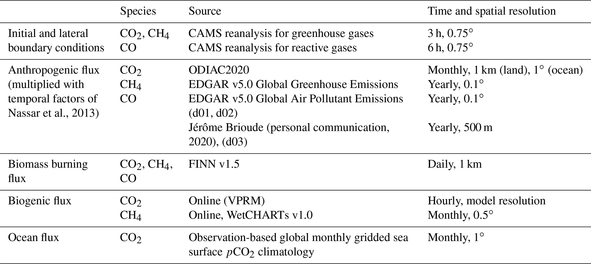
The anthropogenic emissions for CH4 and CO are taken from the Emission Database for Global Atmospheric Research (EDGAR). For CH4, we have used the v5.0 Global Greenhouse Gas Emissions product (Crippa et al., 2019b), while for CO, the EDGAR v5.0 Global Air Pollutant Emissions product (Crippa et al., 2019a) was used. Furthermore, we performed simulations over a short period of a few days to test alternative inventories for anthropogenic CO2 and CO fluxes. We concluded that the Open-Data Inventory for Anthropogenic Carbon dioxide (ODIAC2020; Oda and Maksyuto, 2015, 2011; Oda et al., 2018) was more representative for the anthropogenic CO2 emissions, probably due to its much higher spatial resolution (1 km) compared to EDGAR (0.1∘).
Similarly, we use a CO surface emission inventory at a resolution of 500 m, based on the posterior estimates of a mesoscale inverse model (Jérôme Brioude, personal communication, 2020), but only in the innermost domain d03. The atmospheric transport of the inverse model was calculated using the FLEXPART (FLEXible PARTicle dispersion model) Lagrangian dispersion model (Verreyken et al., 2019) coupled with the Meso-NH mesoscale model (Lac et al., 2018) at a resolution of 500 m and 60 vertical levels. FLEXPART-Meso-NH was run backward in time to calculate the source–receptor relationships between MA and the surface sources from the CO measurements at MA, from 4 April to 3 May 2019, during the BIO-MAIDO (Bio-physico-chemistry of tropical clouds at Maïdo, Réunion Island) campaign (Dominutti et al., 2022). The ODIAC CO2 emission inventory was used a priori to benefit from its native spatial resolution of major urban areas. A scaling factor, based on the ratio between the mean CO enhancement above background and mean CO2 enhancement above background, was applied on the CO2 fluxes to obtain a priori surface CO fluxes. A temporal resolution of 1 h was used for the observed and simulated CO mixing ratios at MA. A lognormal distribution was assumed for the observation and surface flux errors (Brioude et al., 2012, 2013). Such an assumption better matches the CO distribution in the atmosphere and prevents the inversion from calculating negative fluxes.
The anthropogenic fluxes used within WRF-GHG are combined with a temporal emission factor from Nassar et al. (2013). Note that these factors are representative for CO2 and might be less accurate for CO and CH4.
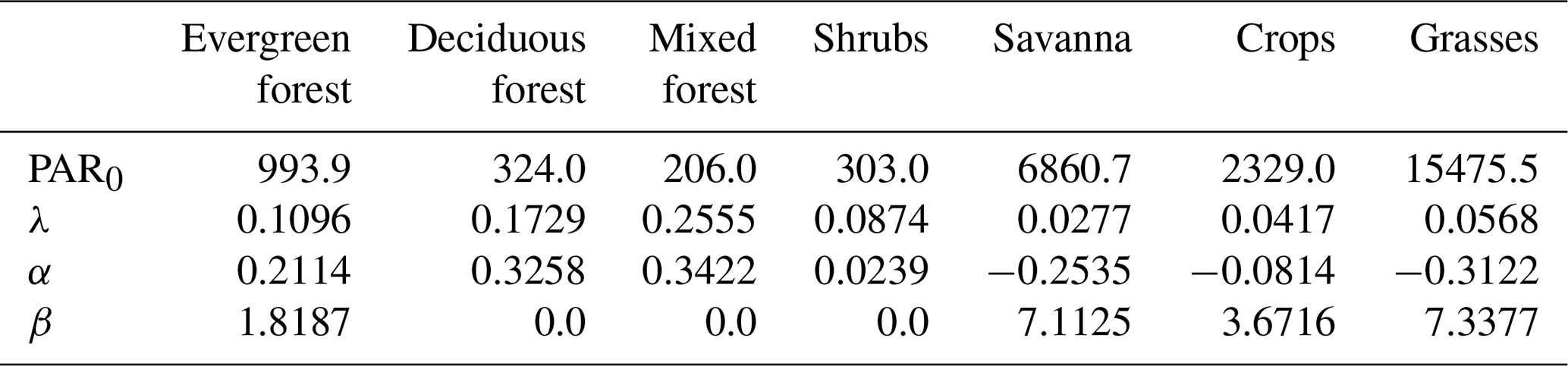
Daily biomass burning emissions for all three gases are obtained from the Fire INventory from NCAR (FINN v1.5; Wiedinmyer et al., 2011). The biogenic CH4 flux from wetlands is obtained from the WetCHARTs v1.0 ensemble (Bloom et al., 2017), while the biogenic CO2 flux from oceans is taken from the observation-based global monthly gridded sea surface pCO2 climatology by Landschützer et al. (2017), which also provides air–sea CO2 fluxes. Finally, the biogenic CO2 flux from the vegetation is simulated online using the VPRM model (Mahadevan et al., 2008; Ahmadov et al., 2007). This model uses the 2 m temperature and downward shortwave radiation calculated by WRF-GHG in combination with surface reflectance data from the Moderate Resolution Imaging Spectroradiometer (MODIS). Furthermore, it uses the global SYNMAP land cover data of 1 km resolution by Jung et al. (2006). Additionally, the VPRM requires a set of four model parameters for each vegetation class, dependent on the region of interest. Ideally, these parameters are optimized using a network of eddy flux towers. Since this is not available at Réunion Island, we use the set of parameters optimized by Botía et al. (2021), based on measurements from nine sites in the Amazon region in Brazil, created in the context of the Large Scale Biosphere–Atmosphere Experiment (LBA-ECO). Exact parameter values are given in Table A1 of Appendix A.
3.2 Settings
To achieve a high-resolution model grid over Réunion Island, a configuration of three nested domains was established, going from a larger domain with a lower resolution to a smaller domain with a higher resolution. The domains are shown in Fig. 2. Their respective resolutions are 50, 10, and 2 km. The innermost domain, d03, covers Réunion Island and the two measurement sites completely. WRF-GHG uses a hybrid vertical coordinate, which is a coordinate that is terrain following near the ground and becomes isobaric higher up. In all our domains, the model has 60 vertical levels extending from the surface up to 50 hPa.
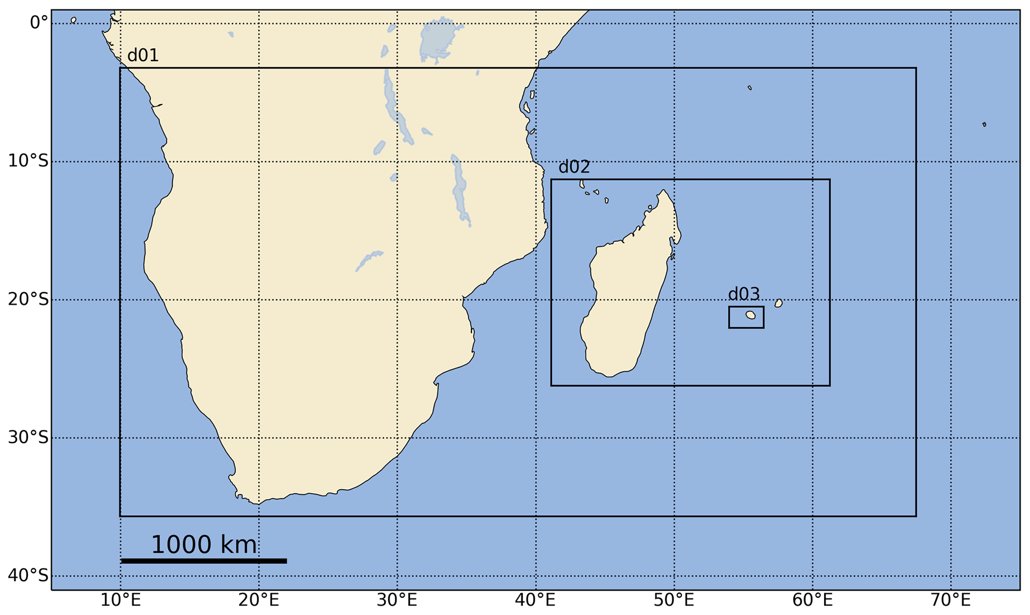
Figure 2Location of the WRF-GHG domains, with horizontal resolutions of 50 km (d01), 10 km (d02), and 2 km (d03). All domains have 60 (hybrid) vertical levels extending from the surface up to 50 hPa.
The following physical parameterization options are used: the Morrison two-moment scheme (Morrison et al., 2009) for microphysics, the Rapid Radiative Transfer Model for general circulation models (RRTMG) shortwave and longwave schemes (Iacono et al., 2008). The Eta similarity scheme (Janjić, 1994) for surface layer processes and the Unified Noah LSM (land surface model; Tewari et al., 2004) for the land surface. To choose between the diverse parameterization schemes for cumulus parameterization and planetary boundary layer (PBL) physics, several model test runs were made for a short simulation period of a couple of days and compared with the observed meteorology. As a result, the University of Washington turbulence kinetic energy (TKE) boundary layer scheme (Bretherton and Park, 2009) for PBL physics and the Grell–Freitas ensemble scheme (Grell and Freitas, 2014) for cumulus parameterization, but only in the largest domain (d01), were chosen for this study.
3.3 Data handling
The various observation types are dealt with in different ways for comparison with the model.
The surface observations (both meteorological fields and GHGs) are averaged over a period of 30 min around the hourly model time step. At SDe, we compare these data with the lowermost level of the model grid cell, whose center is closest to the location of the instrument. Because of the complex topography, the cell covering MA is less representative for the observatory, as its center is located behind the summit, in the caldera of Cirque de Mafate below. Model–data comparisons of the surrounding cells showed that the cell to the west of MA is more representative. Therefore, this alternative model grid cell, of which the center is only 1.3 km away from the observatory, is used in the analysis.
In order to compare similar quantities, the total column-averaged dry air mole fractions from TCCON and NDACC are truncated to the same atmospheric column that is simulated by WRF-GHG, e.g., from surface up to 50 hPa. This is needed because the FTIR data represent the total atmospheric column, whereas the WRF-GHG upper limit lies at around 21 km.
As NDACC additionally provides volume mixing ratio profiles, the column-averaged mole fractions are recalculated by taking only those layers below the model upper limit. For TCCON, only information on the total column is retrieved. Therefore, we multiply the TCCON data with a factor representing the ratio between the column-averaged mole fraction of the smaller column (up to 50 hPa) to that of the total column. This ratio is calculated from the a priori information. In the rest of this paper, all dry air column-averaged mole fractions (so-called Xgas) mentioned refer to this reduced atmospheric column only (surface up to 50 hPa). Due to the specific profile of the respective gases in the atmosphere, this scaling is more significant for XCH4 than it is for XCO or XCO2; the values generally increase after scaling by about 27–35 ppb for XCH4, 3 ppb for XCO, and 0.25 ppm for XCO2.
To compare with the hourly WRF-GHG outputs, the scaled mole fractions are averaged over a period of 30 min around the model time step. Furthermore, a smoothing is applied to the WRF-GHG profiles, according to Rodgers and Connor (2003). Because of the different characteristics of the TCCON and NDACC observing systems, this smoothing procedure is slightly different at the two sites. Technical details on how the smoothed dry air column-averaged mole fractions of WRF-GHG are calculated at SDe and MA can be found in Appendix B.
4.1 Meteorological evaluation
4.1.1 Surface measurements
To assess the general model performance, the hourly model output of d03 near the surface is compared with local measurements of 2 m temperature and 10 m wind direction and speed at both sites. Table 2 gives the root mean square error (RMSE), mean bias error (MBE), and Pearson correlation coefficient (CORR) of the model–data comparison over the complete time series (13 583 paired data points at SDe; 14 031 at MA).
Table 2Overview of the meteorological evaluation of the surface measurements at the two sites. The root mean square error (RMSE), mean bias error (MBE), and Pearson correlation coefficient (CORR) are shown.
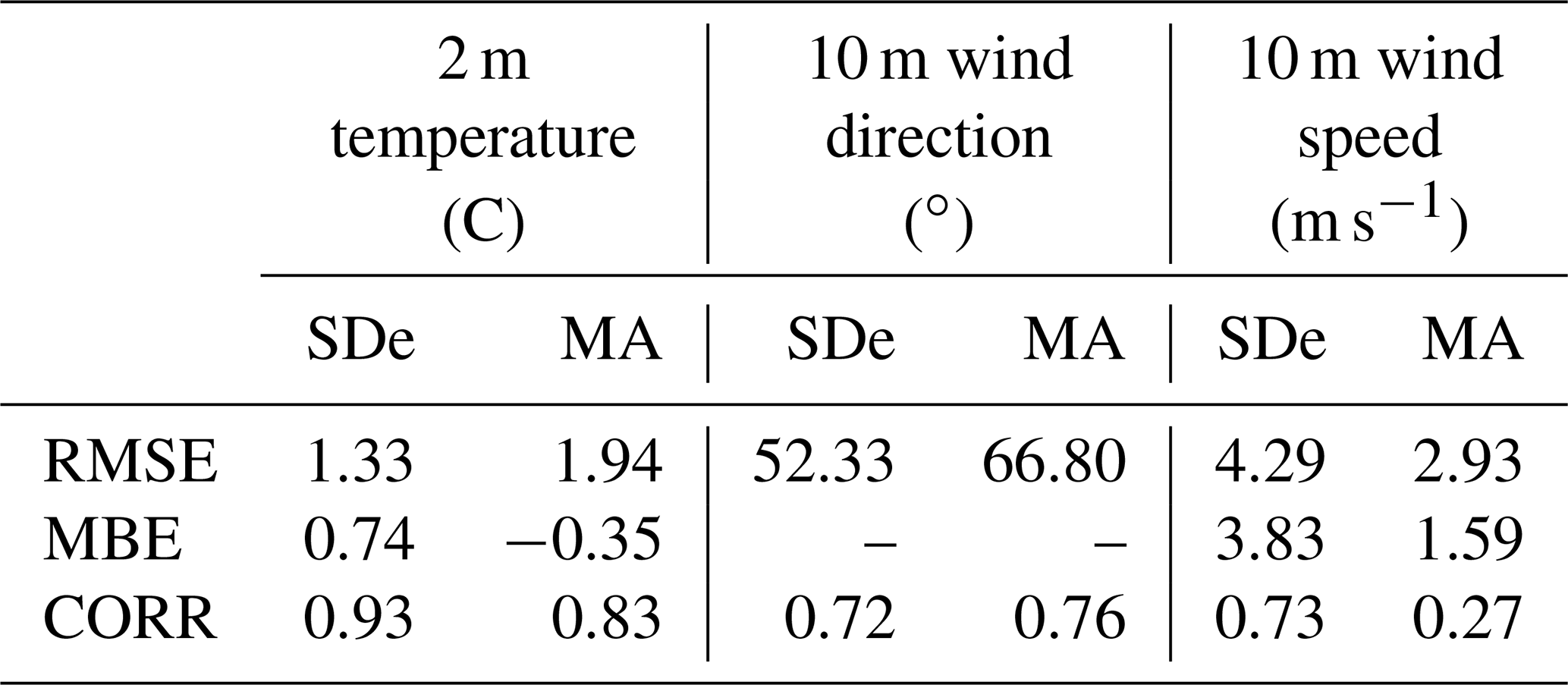

Figure 3(a–b) Diurnal cycle of the 2 m temperature and (c–d) 10 m wind speed at both SDe and MA. The blue and black lines show the median values for every hour of the measurements and simulations, respectively. The shaded blue and gray areas indicate the corresponding interquartile ranges of the measurements and simulations, respectively. Hours are given in UTC (local time at Réunion Island is UTC+4). Note that the temperature plots have different y axes.
The 2 m temperature is well simulated by WRF-GHG at both sites with very high correlation coefficients of 0.93 at SDe and 0.83 at MA and RMSE between 1 and 2 ∘C (1.33 at SDe, 1.94 at MA). Figure 3a–b compare the median diurnal cycle at both sites, which is very well reproduced by the model. Overall, higher temperatures are measured at SDe compared to MA because of the large difference in altitude between the sites (85 m a.s.l. compared to 2155 m a.s.l.).

Figure 4Wind rose from observations and WRF-GHG simulations at SDe (a–b) and at MA (c–d). The colors indicate the associated wind speed (in m s−1), while the lengths of the bars show the frequency of any wind direction binned by 15∘, given in percentage.
The wind roses in Fig. 4 show the most-occurring 10 m wind directions and their corresponding wind speed. The 10 m wind direction of WRF-GHG correlates well with the measurements at both sites (correlation coefficients of 0.72 and 0.76). There is a larger error of the wind direction at MA (RMSE of 66.80∘) compared to SDe (RMSE of 52.33∘). At SDe, the wind is mainly from the east or southeast (trade winds); however, for calmer wind speeds (< 2 m s−1), the wind can also come from the south(west). WRF-GHG captures the dominant southeastern winds but does not simulate winds from the south. It highly overestimates the wind speed, with a mean bias error of 3.83 m s−1 and a RMSE of 4.29 m s−1. There is a clear diurnal cycle of the wind speed at SDe, shown in Fig. 3c, with stronger winds during the day and calmer conditions at night. As WRF-GHG follows the observed pattern, the correlation coefficient is still quite high (0.73). The overestimation might be caused by an underestimation of the surface roughness of the city within WRF-GHG. Besides the unified Noah land surface model (see Sect. 3.2), no additional urban surface model was included in the simulations. Other studies using the WRF model often show wind speed overestimation above urban areas (Feng et al., 2016; Barlage et al., 2016; Zhang et al., 2009; Kim et al., 2013). Additionally, there is a large gradient in the surface wind speed near SDe caused by the presence of the strong trade winds. Therefore, an insufficient high model resolution might also be the cause for the wind speed overestimation.
At MA, on the other hand, the most common wind direction is east with some occurrences of westerly winds. This points to the typical thermally induced circulations during the day, whereby wind is driven from the coast upwards and sometimes reaches MA (Duflot et al., 2019). The prominent east winds illustrate the presence of overflowing trade winds. The simulated winds from WRF-GHG are mainly from the east, indicating that the larger errors at MA might be linked to the missing westerly wind components. This is likely due to the complex topography around the Maïdo Observatory and the model resolution (of 2 km), which might be insufficient for resolving these very local wind dynamics.
As to the wind speed at MA, the bias and RMSE are smaller (1.59 and 2.93 m s−1, respectively) than at SDe, but the model is still overestimating the wind speed. Moreover, the correlation is very low at this site. The daily 10 m wind speed cycle at MA is less distinct than at SDe; however, at night the wind is more often faster (> 2 m s−1) than during the day. This could be linked to the local wind dynamics around MA, where calmer upslope winds from the west often reach MA during the day, while at night the observatory is generally in the free troposphere under the influence of the faster trade winds (Guilpart et al., 2017).
4.1.2 Radiosonde profile measurements
Daily radiosonde profiles of air temperature, wind direction, wind speed, and relative humidity are compared with the model data to assess the accuracy of WRF-GHG on all levels of the troposphere. The profiles were matched as follows: for every data point measured by the radiosonde, the grid cell corresponding to its coordinate is selected. Next, the model profile (consisting of the meteorological field in the complete vertical column above the selected grid cell) is interpolated to the altitude of the measurement. This interpolated value is then paired with the value of the measurement. This results in a paired model–data profile for the four variables once every day. An example of such a paired profile on 5 July 2016 is shown in Fig. 5. For every paired profile, the RMSE, MBE, and CORR statistics are calculated. This is done for a total of 267 d in the year 2016.
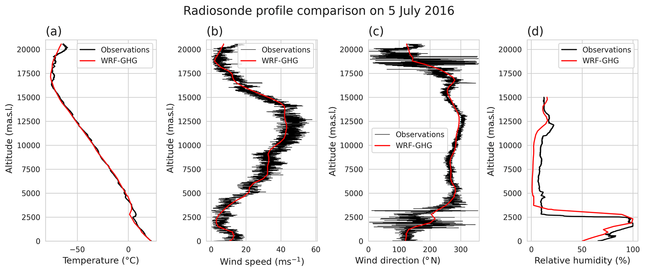
Figure 5Example of the radiosonde data at Roland Garros Airport on 5 July 2016, compared with the model for (a) temperature, (b) wind speed, (c) wind direction, and (d) relative humidity. The black line represents the measured values. The red line is the corresponding WRF-GHG data.
For the temperature, correlation coefficients are very high on all days (median is 0.99). Moreover, the RMSE values are quite small on most days (median is 1.07 ∘C), indicating that WRF-GHG can simulate the temperature in the troposphere quite accurately.
There is a good correlation for the wind direction and speed profiles as well. Half of the days in 2016 have a correlation coefficient higher than 0.87 for wind direction and 0.83 for wind speed. When calculating the RMSE of wind direction along the daily profiles, we find a median of 48.18∘, while the median RMSE of the wind speed is 3.87 m s−1. On most days, WRF-GHG is slightly underestimating the wind speed (median bias error is −1 m s−1), which is in contrast with the overestimation found at the surface sites.
The profiles of relative humidity are analyzed up to an altitude of 15 km because the measurements are less accurate higher up. WRF-GHG correlates well with these profiles, with a correlation coefficient higher than 0.87 on 75 % of the days in 2016. The median RMSE on the daily profiles of relative humidity is only 11.6 %, showing a decent model performance.
Overall, we can conclude that the simulations of basic meteorological parameters are quite accurate along vertical profiles, where near the surface wind speed and direction agree less well with the observations.
4.2 GHG data at Saint-Denis
At SDe, the in situ surface mole fractions of CO2 and CH4 are measured together with the TCCON column-averaged dry air mole fractions of CO2, CH4, and CO. The comparison with the WRF-GHG simulations will be described in detail below, for each species and measurement type separately. The full time series of the observed and modeled data can be found in Appendix C. An overview of the statistics of the comparisons is given in Table 3.
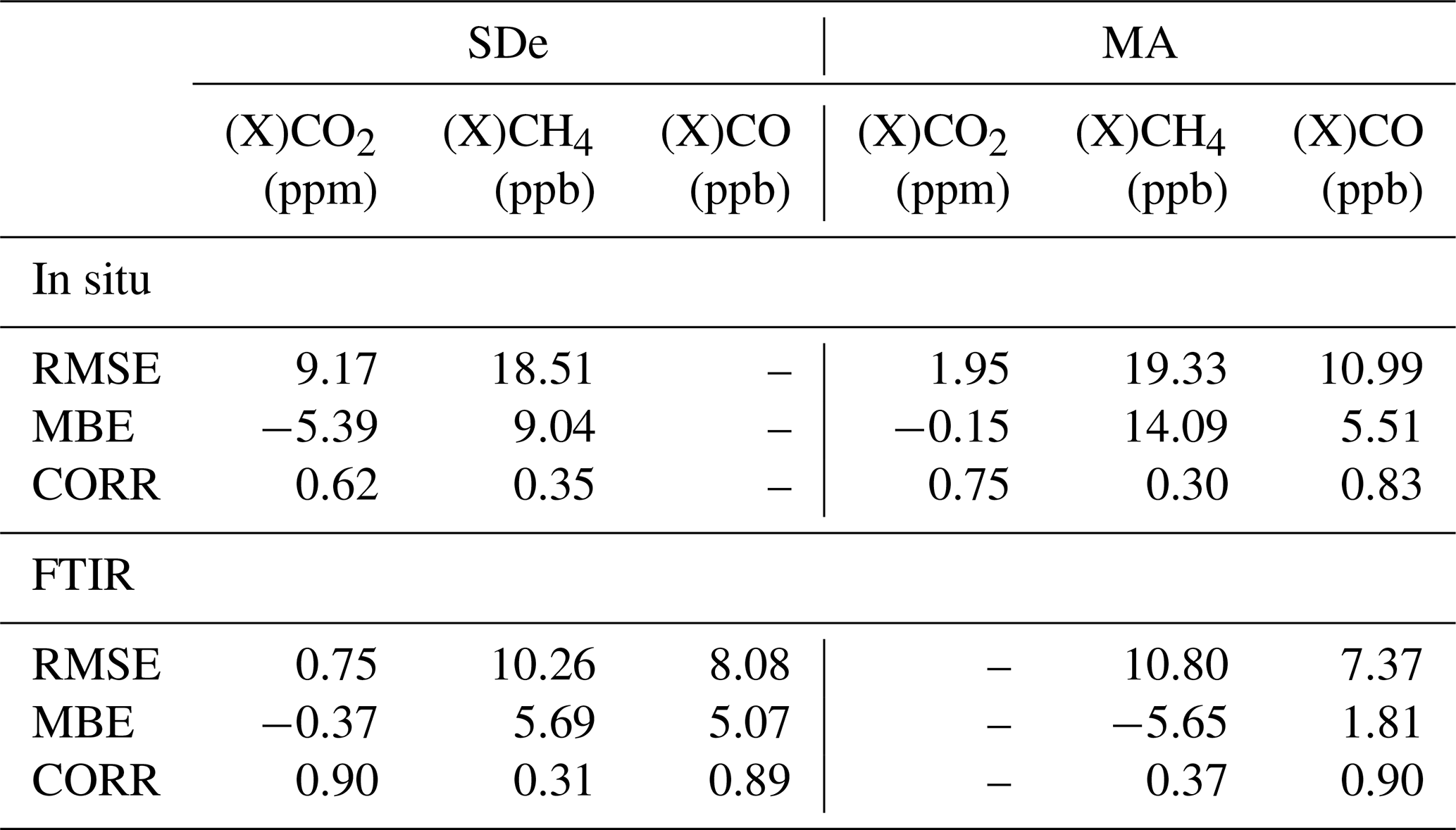
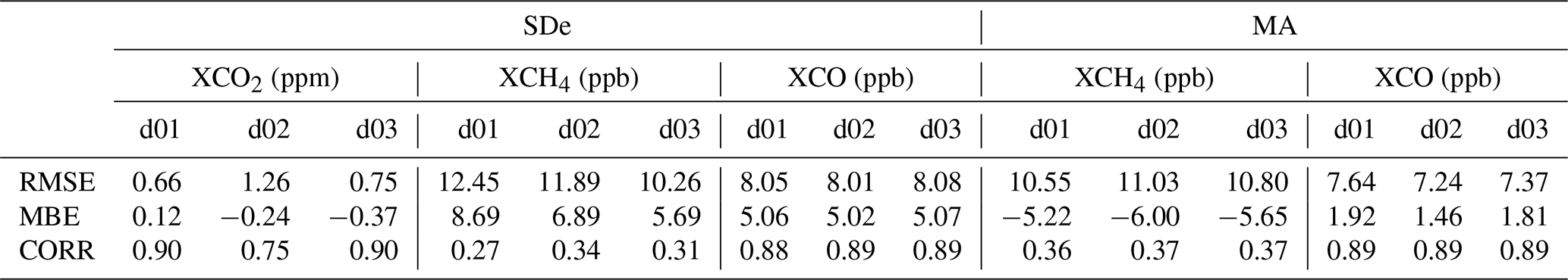
Table 3Overview of the WRF-GHG performance for hourly in situ and column observations of GHG at Réunion Island. The comparison with the column observations is based on the smoothed model profiles. There are no in situ CO data available at SDe (Saint-Denis) and no XCO2 data at MA (Maïdo).
4.2.1 Surface CO2
The model–data comparison of the surface data shows a moderate correlation coefficient of 0.62 together with a relative large error of 9.17 ppm and a model underestimation of 5.39 ppm. The scatterplot in Fig. 6a indicates that these discrepancies arise from a model underestimation of the higher CO2 mole fractions. The lower CO2 concentrations are, in general, much better reproduced.
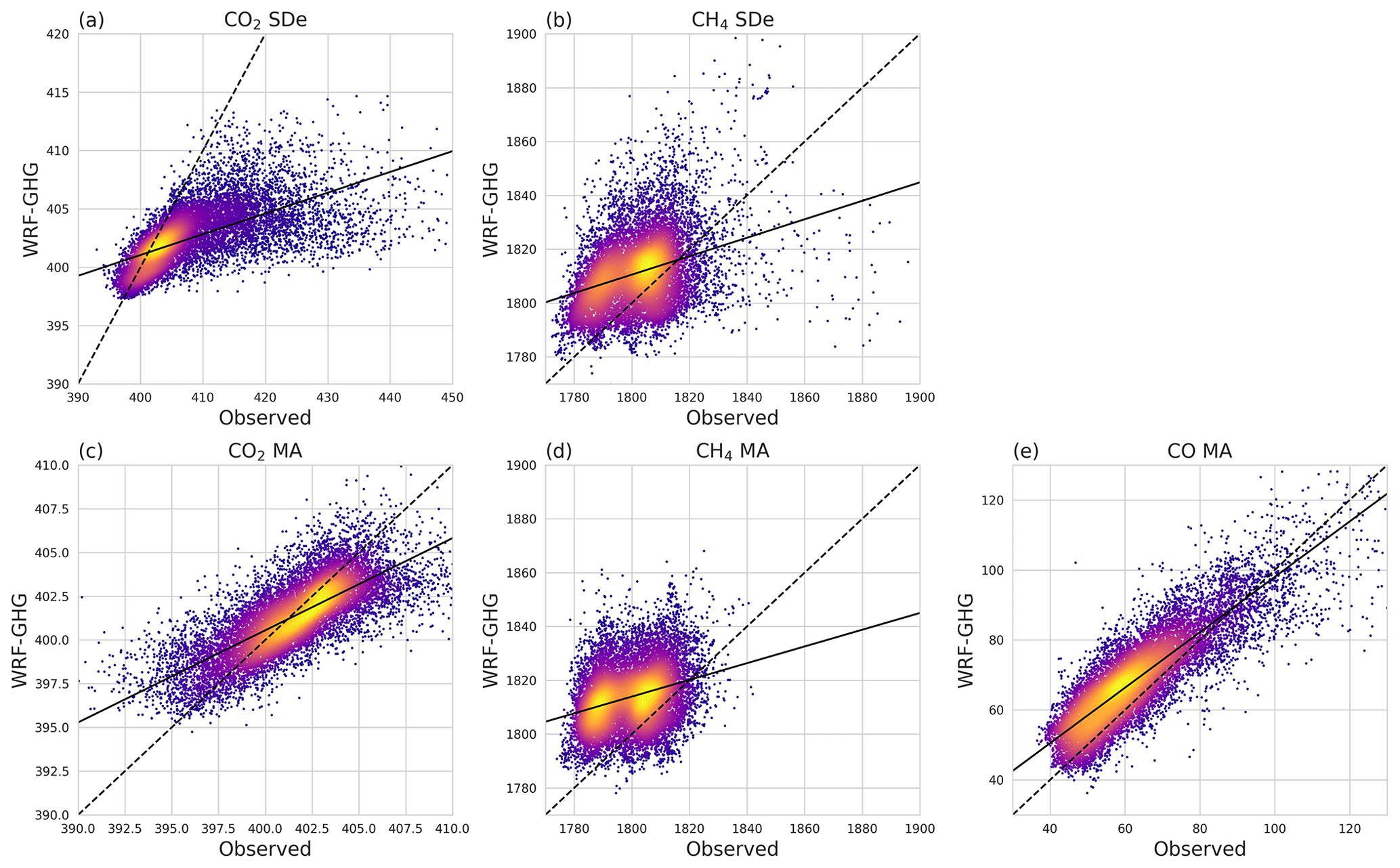
Figure 6Scatterplot of hourly observed and modeled in situ greenhouse gases at SDe (a, b) and MA (c, d, e). The colors indicate the point density.

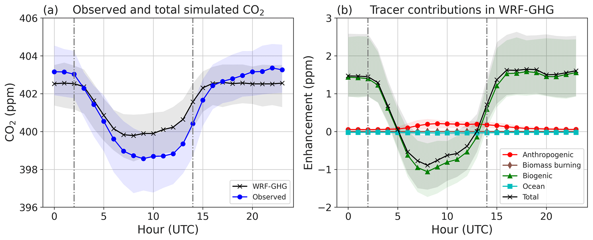
Figure 7Diurnal cycle of (a) in situ CO2 at SDe (b) and model tracer contributions. The black line in panel (a) represents the median hourly concentrations of WRF-GHG, while the blue line represents the observed values. The shaded areas cover the interquartile ranges. The gray dotted vertical lines at 02:00 and 14:00 UTC indicate the approximate times of sunrise and sunset. The colored lines in panel (b) represent the different tracer deviations from the background concentration in WRF-GHG, including anthropogenic (red), biogenic (green), ocean (cyan), and biomass burning (brown) tracers. The black line is the sum of all tracers, except the background.
The CO2 measurements at SDe show a clear diurnal cycle (see Fig. 7a), with lower values during the day and higher values during the night. The diurnal cycle of WRF-GHG reproduces this pattern but with much lower nighttime concentrations, leading to the moderate correlation found in Table 3.
As shown in the diurnal cycle in Fig. 7b, the main contributors to the total CO2 signal in WRF-GHG, in addition to the background signal, are the anthropogenic and biogenic tracers. They correspond with anthropogenic and biogenic fluxes within the model domains (d01–d03) and show similar diurnal patterns with maxima at night and minima during the day. The influence of biomass burning or ocean fluxes is negligible at SDe.
In urban areas, anthropogenic pollution is generally trapped in and around the city, creating a so-called urban CO2 dome (Idso et al., 2002). The strength of this dome is primarily dependent on the local emissions and variations in the boundary layer. In calm weather, near-surface air temperature inversions at night trap anthropogenic pollution near the ground in the shallow nocturnal boundary layer, leading to strongly enhanced CO2 mixing ratios. During the day, solar radiation causes convective mixing of the air, creating a deep planetary boundary layer (PBL). The near-surface CO2 concentrations are then diluted by this thorough mixing of air, and the urban dome extends to greater heights.
However, wind speed and direction can alter the strength of this urban CO2 enhancement; at higher wind speeds (from 2 m s−1), ventilation processes prevent strong CO2 accumulation, while winds from rural areas could bring pristine air to the city (Idso et al., 2002; Rice and Bostrom, 2011; Massen and Beck, 2011; García et al., 2012; Xueref-Remy et al., 2018).
Within WRF-GHG, the main contributors to the simulated CO2 in the grid cells around SDe are anthropogenic and peak during the day. The biogenic CO2 flux at the grid cell of SDe is zero because the corresponding VPRM vegetation class is 100 % barren, urban, and built-up. Thus, the model assumes that there is no vegetation within the city. Given that Saint-Denis is the capital city of Réunion Island and has plenty of anthropogenic activities, the impact of local vegetation is probably very small, and these WRF-GHG fluxes appear realistic. The nighttime peak of CO2 mixing ratios is therefore attributed to PBL dynamics and regional transport.
Figure 7a shows that the observed interquartile range at night is wide, indicating a large variability in the CO2 accumulation. We find a negative correlation between 10 m wind speed and in situ CO2 concentrations at night for the observations at SDe (see Fig. 8). At low wind speeds, a large variability in CO2 mixing ratios is observed from 400 up to 450 ppm. For wind speeds above 2 m s−1, on the other hand, values higher than 410 ppm are rarely found, which indicates that ventilation processes take place. At the same time, there is a large overestimation of the wind speed within WRF-GHG (Sect. 4.1.1; Table 2). At night, 91.7 % of the simulated hours has a wind speed of more than 2 m s−1, compared to only 23.2 % of the nocturnal observations, leading to a wind speed MBE of 3.23 m s−1 at night. Note that the mean wind speed at night within WRF-GHG is 4.4 m s−1 (see also Fig. 3c), while the nighttime CO2 concentration in WRF-GHG is on average 403.8 ppm (see also Fig. 7a). Looking at Fig. 8, these values follow the pattern as found in the observations, where a nocturnal wind speed of more than 4 m s−1 corresponds with CO2 mole fractions of about 403–404 ppm. Therefore the model is likely underestimating the in situ CO2 observations at SDe because of an overestimation of the surface wind speed.
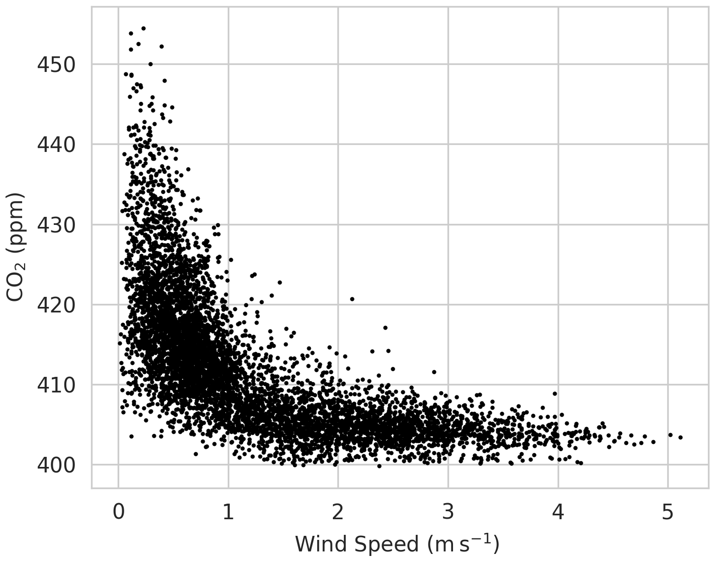
Figure 8Scatterplot of nighttime wind speed at SDe against hourly observed in situ CO2. Nighttime hours are defined as those between 14:00 and 02:00 UTC.
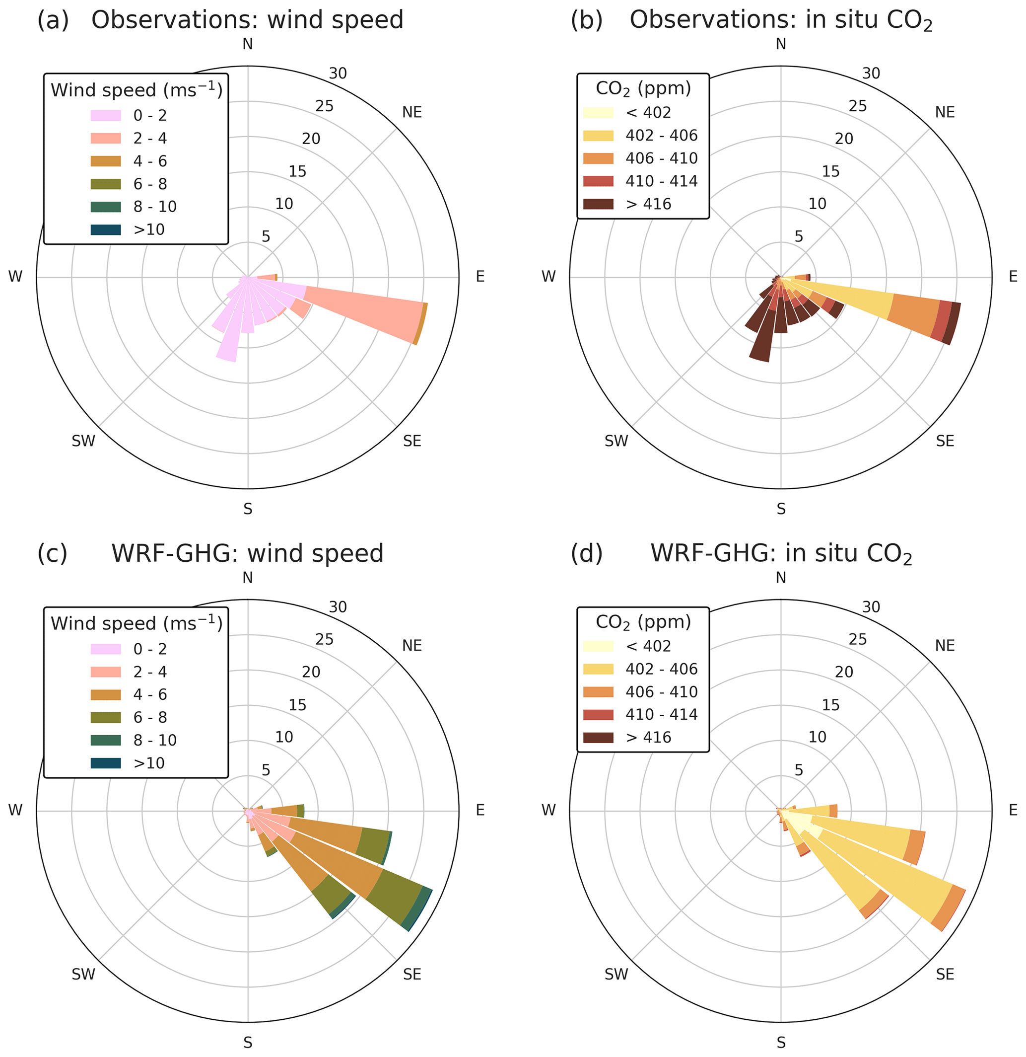
Figure 9Wind rose of hourly nighttime data at SDe, where the night is defined between 14:00 and 02:00 UTC. Panels (a) and (b) show the distribution of the observed wind speed per wind direction and near-surface CO2 concentration per wind direction, respectively. Panels (c) and (d) show the same for WRF-GHG simulated data. The lengths of the bars show the frequency of occurrence in percentage.
Furthermore, we examine the relation of nighttime CO2 concentrations and 10 m wind direction at SDe. Figure 9a shows that the dominant observed wind direction at night is easterly–southeasterly (ESE), followed by southerly (S). The ESE winds generally correspond with higher wind speeds (> 2 m s−1) and lower CO2 concentrations (generally below 410 ppm), whereas observations with southerly winds generally coincide with very low wind speeds and CO2 accumulation (Fig. 9a and b). The region in the ESE of SDe is a rural area dominated by agricultural activities. Therefore, these stronger ESE winds would generally bring air with a lower CO2 content to SDe. WRF-GHG, on the other hand, overestimates the wind speed and almost consistently simulates ESE winds and lower CO2 concentrations (Fig. 9c and d). As such, the model–data mismatch is likely caused by a combination of both wind speed overestimation in WRF-GHG and discrepancies as to the wind direction, which are interrelated.
4.2.2 XCO2
A higher correlation coefficient of 0.90 is found when comparing the daytime hourly averaged TCCON XCO2 data with the smoothed XCO2 from WRF-GHG (see Table 3). Moreover, the RMSE along the time series is 0.75 ppm, and there is a model underestimation of 0.37 ppm. The hourly relative model–data errors are below 0.5 % (Fig. 10). This is, however, slightly larger than the TCCON standard deviation of the hourly averages, which is around 0.1 %.
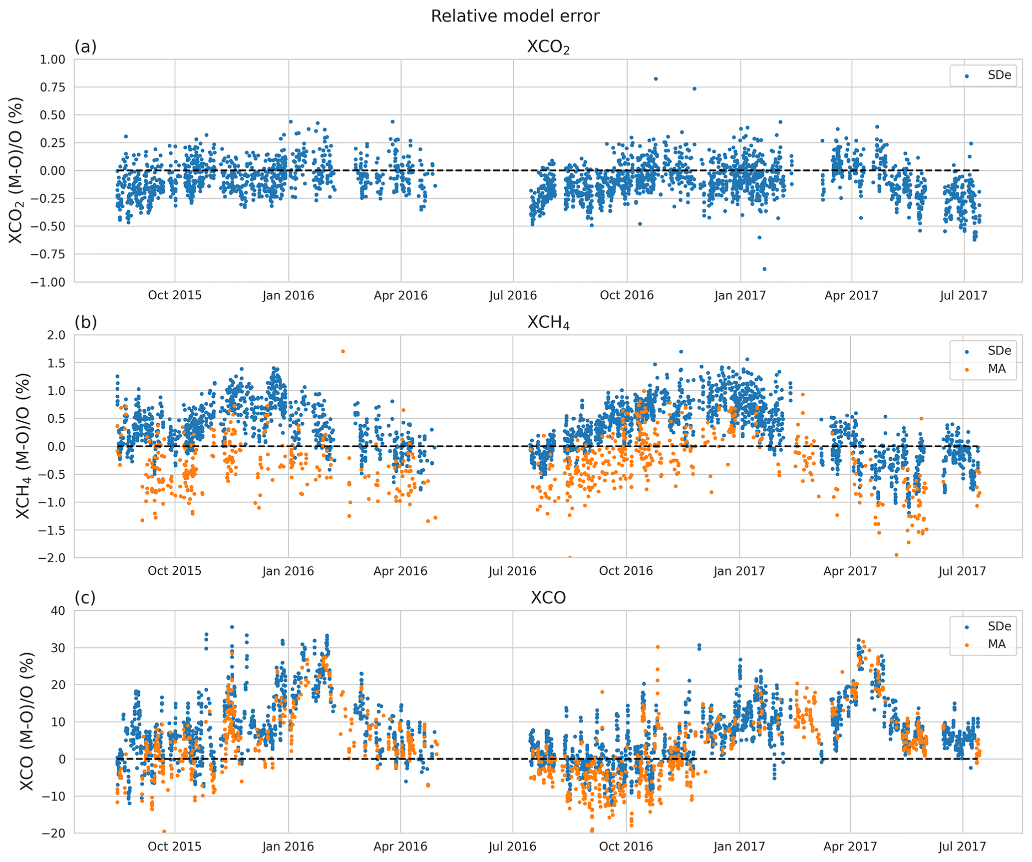
Figure 10Relative percentage differences between hourly (smoothed) WRF-GHG and FTIR observations of XCO2, XCO, and XCH4. The blue dots represent the data at SDe (WRF–TCCON), while the orange data are from MA (WRF–NDACC).
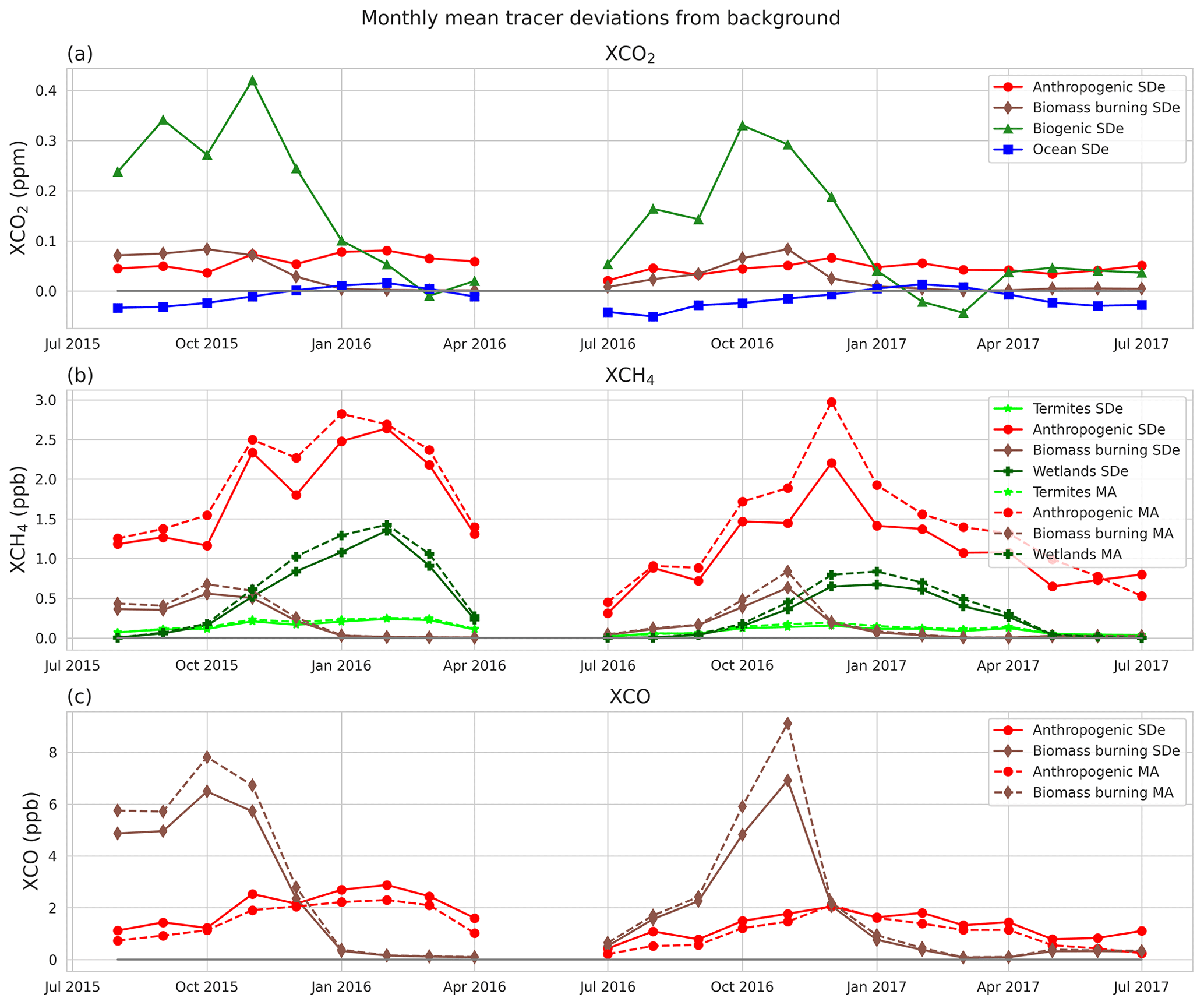
Figure 11Monthly mean tracer contributions to the column-averaged mole fractions of (a) CO2, (b) CO, and (c) CH4. The different colors represent different tracers, i.e., anthropogenic (red), biogenic (green), ocean (blue), wetlands (dark green), termites (light green), or biomass burning (brown). The solid lines are the mean monthly contributions at SDe, while the dashed lines are for MA.
WRF-GHG provides a separation into different tracer contributions, which are shown in Fig. 11. Monthly averages of these contributions for XCO2 show a large (positive) biogenic enhancement in the months from August to December. The biogenic tracer in WRF-GHG is driven by the online biogenic CO2 fluxes calculated through the VPRM module as the sum of the gross ecosystem exchange (GEE) and respiration (Mahadevan et al., 2008). A positive biogenic tracer suggests that the respiration accumulates more CO2 than the ecosystem can capture during the day by photosynthesis. Indeed, in the Southern Hemisphere, the dry season is generally from May until November, leading to a decrease in GEE in some ecosystems (Quansah et al., 2015; Räsänen et al., 2017). Moreover, this carbon source was higher in 2016 because of a strong El Niño–Southern Oscillation (ENSO) event, leading to higher temperatures and less precipitation in the tropics (Yue et al., 2017).
The anthropogenic enhancement is relatively constant throughout the year. There is also a small biomass burning component modeled in XCO2 in the months from August to December, which corresponds to the biomass burning (BB) season. During these months, frequent fires occur in southern Africa and South America. Duflot et al. (2010) showed that these polluted air masses can be transported to Réunion Island and detected by FTIR observations, such as XCO. Note that the XCO2 enhancements due to biomass burning coincides with the biogenic enhancements because, especially in the tropics, the occurrence and duration of the BB season are linked to the dry season (Giglio et al., 2006).
A recent study using a COCCON spectrometer at Gobabeb in Namibia showed that the African biosphere can impact the observed XCO2 signal there due to medium- and long-range transport (Frey et al., 2021). More specifically, they demonstrated that the carbon sink of the African biosphere during austral summer can be observed in their XCO2 measurements, while it is not (or to a lesser extent) visible in the time series at Réunion Island. Backward trajectories for 1 specific day in February 2017 revealed that this contrast comes from the sampling of different air masses. This might suggest that the influence of fluxes from the African continent on the air above Réunion Island is seasonally dependent, with a high impact during the dry season and a lower impact during wet season. Backward trajectory simulations over a longer time period performed by Zhou et al. (2018) might suggest this as well; however, more research is needed to prove this statement.
As expected, the column observations of CO2 are determined by different processes than the in situ CO2 concentrations. Where the variation in XCO2 is mainly driven by fluxes on the African continent, the surface CO2 mole fractions are heavily influenced by local sources and PBL dynamics. This also agrees with the trajectory calculations by Zhou et al. (2018), showing that surface air mainly originates in the Indian Ocean, while free tropospheric air is mainly coming from Africa and South America.
4.2.3 Surface CH4
The model–data comparison for CH4 at SDe (Table 3) shows only a weak correlation (0.35) between modeled CH4 and observations at SDe. WRF-GHG shows an overestimation of about 9 ppb. Figure 6b and d show two apparent distributions in the scatterplot. This is linked with the seasonal cycle of CH4, where observations show minimum values in December–February and maximum values in August–September. The errors between the observations and WRF-GHG are not constant over time. In Fig. 12, a seasonal bias is found, with larger errors between December and February, which is austral summer. This is a known weakness in the CAMS reanalysis, used as boundary information, as pointed out in the most recent validation report by Ramonet et al. (2020).
For all observations CH4 shows a seasonality in the relative difference between observations and CAMS simulations, which is increasing in the Southern Hemisphere after 2008. … The seasonal dependence, which needs to be investigated in more detail, may be related to the representation of OH in the model, or/and to errors in the seasonal cycle of surface emissions (mainly from agriculture and wetlands). (Ramonet et al., 2020)
This demonstrates the importance of accurate lateral boundary conditions for simulating long-lived tracers with regional models such as WRF-GHG.

Figure 12Time series of daily mean relative percentage differences between model and in situ observations of CH4 at SDe (orange) and MA (blue). The black dashed line indicates zero difference.
The diurnal cycle of the CH4 tracer contributions in Fig. 13 shows that the modeled CH4 consists almost entirely of the background signal and an anthropogenic enhancement, whereby both factors can add to the model–data mismatch.
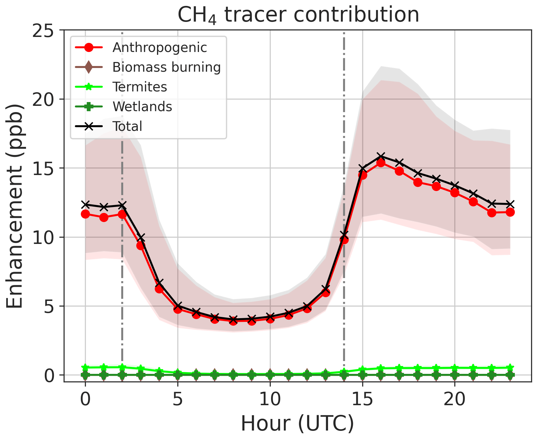
Figure 13Diurnal cycle of in situ CH4 tracer contributions of WRF-GHG at SDe. The black crosses represent the median hourly enhancements above the background for the sum of all tracers. The separate tracer contributions are given in red (anthropogenic), dark green (wetlands), light green (termites), or brown (biomass burning). The shaded areas cover the interquartile ranges. The gray dotted vertical lines at 02:00 and 14:00 UTC indicate the approximate times of sunrise and sunset.
The diurnal cycle is less pronounced in the observations (not shown). Nighttime values are on average only slightly larger than during the day, with a mean difference of only 3.09 ppb (σ2=6.35), indicating that a nocturnal accumulation as identified for CO2 in Saint-Denis is less evident for CH4. Moreover, the overestimation of the daily amplitude in WRF-GHG suggests an overestimation of the local anthropogenic CH4 fluxes from EDGAR.
In contrast to CO2, the CH4 mole fractions near the surface are less impacted by PBL dynamics and more by the background concentration.
4.2.4 XCH4
Incorrect boundary values and hence background concentrations have an impact on all CH4 simulations at Réunion Island. Therefore, the statistics for the column-averaged mole fraction of XCH4 at SDe (part of TCCON) are worse than for CO2. A weak correlation is found (0.31; Table 3), and the model overestimates TCCON XCH4 by 5.69 ppb, which is slightly less than the bias with respect to in situ data (Sect. 4.2.3).
Figure 10c shows the relative differences between WRF-GHG and observational data, which have the same seasonal pattern as for the in situ comparisons (Fig. 12) caused by the reported seasonal bias for CH4 in the CAMS reanalysis data. The relative differences are below 2 %, but due to this seasonality in the errors, very little correlation is found.
Even though the model fails at reproducing the measured time series, it is still interesting to examine the different modeled tracer contributions to XCH4 (Fig. 11b). The tracers contribute only a few ppb to the total signal, with the anthropogenic being dominant throughout the year. Furthermore, small peaks in biomass burning enhancements are found during the BB season, as for the other species. The biogenic tracers for CH4 in WRF-GHG are generated by emissions from termites and wetlands. The termite signal is, however, very small and thus not relevant for this region. The signal from wetlands is larger, especially in austral summer. This roughly coincides with the rain season, causing a greater wetland extent (Lunt et al., 2019).
In the same way as for CO2, the surface CH4 mole fractions at SDe are influenced by local sources at Réunion Island, while fluxes from Africa and Madagascar are detected in the column observations because of the different air masses they sample.
4.2.5 XCO
At SDe, CO is only available as a column-averaged mole fraction (part of TCCON). As seen in Table 3, a very high correlation (0.89) is found for the hourly averaged paired data. WRF-GHG slightly overestimates the observed XCO (MBE of 5.07 ppb). Figure 10c shows that the relative error between WRF-GHG and the XCO observations from TCCON is often below 20 % but not constant because larger errors up to 30 % are found from January until May.
As for the other species, large contributions of BB emissions are found in the months from August to December (Fig. 11c). Duflot et al. (2010) showed that XCO values during the BB season can reach up to twice the CO background concentration from other months. The rather limited BB enhancement found in WRF-GHG suggests that a substantial XCO increase in the BB season is already included in the background tracer. This suggests that fires outside of the large domain can also be detected at Réunion Island, such as those from South America, which would confirm the findings of Duflot et al. (2010). The anthropogenic contribution is more constant throughout the year, and it is the dominant contribution outside BB season. However, it remains rather small compared to the background, which appears to be the main driver behind the simulated XCO values at Réunion Island.
The larger model overestimations in January 2016 and April 2017 are thus likely linked to the background tracer, which is based on the CAMS global reanalysis for reactive gases. The corresponding CAMS validation report (Errera et al., 2021) mentions no known biases but shows similar relative errors in those months in the Southern Hemisphere and in particular at MA (visible in Errera et al., 2021; see their Fig. S6 on p. 10). Again this demonstrates the importance of accurate boundary conditions for simulating XCO in this region but additionally points to the large influence of remote regions (outside domain d01) on the observed XCO time series at Réunion Island.
4.3 GHG data at Maïdo
At MA, the surface mole fractions of all three gases (CO2, CH4, and CO) are measured together with the column-averaged mole fractions of CH4 and CO that are part of NDACC. The results of each species are given in the sections below. Again, the full time series of the observed and modeled data can be found in Appendix C, and statistical metrics of the model–data comparison are shown in Table 3. Note that all statistical analyses of in situ observations at MA are performed on the complete data set. Studies at other high-altitude stations often filter only those measurements which are representative for the free troposphere (Sepúlveda et al., 2014). However, analyses comparing only day- or nighttime data at MA showed no significant differences in the results.
4.3.1 Surface CO2
At MA, the in situ CO2 observations by the Picarro instrument are well reproduced by WRF-GHG, resulting in a correlation coefficient of 0.75 and a very small MBE of −0.15 ppm (see Table 3). As at SDe, the diurnal CO2 cycle at MA shows a daytime minimum and a nighttime maximum (see Fig. 14a); however, the amplitude is much smaller. This pattern is caught by WRF-GHG, although the amplitude is slightly underestimated. During the day, WRF-GHG shows a small overestimation of the CO2 measurements of about 0.9 ppm, while at night a slight underestimation (about 0.4 ppm) is found. As seen on Fig. 14b, the modeled diurnal variation is almost entirely produced by the biogenic tracer, indicating that the biogenic flux calculated by VPRM might be the reason for the model–observation discrepancies. The VPRM parameters used in the model are based on model tests in the Amazon region.
Foucart et al. (2018) showed that, due to surface radiative cooling, the observatory is primarily situated in the free troposphere at night. The air at MA is then disconnected from local pollution sources, and air from remote regions can be sampled. Indeed, no anthropogenic contribution is detected during the nighttime. However, the observed and simulated diurnal cycle of CO2 (Fig. 14a and b) shows that nighttime measurements at MA are still influenced by the respiration of the local vegetation.
The anthropogenic contribution at MA is very minor in WRF-GHG, which is expected because of the remote location of the observatory. A very small enhancement is identified during the day. Since the local grid cell used for the model comparison does not include any anthropogenic flux, this enhancement is advected from elsewhere. It has been shown that orographic lifting can bring polluted air from coastal areas in the west towards MA during the day (Foucart et al., 2018; Duflot et al., 2019). Despite the fact that these westerly winds during the day were not reproduced by WRF-GHG (see Sect. 4.1.1), a daytime anthropogenic enhancement is found in the simulations. The model components representing biomass burning and ocean fluxes at MA are negligible.
So, according to WRF-GHG, the main contribution (above the background) to the CO2 signal at MA is coming from the local vegetation and its photosynthesis and respiration, leading to a distinct diurnal cycle. The importance of the surrounding biosphere for the surface observations at MA was also found by Verreyken et al. (2021), for volatile organic compounds. Even though the diurnal cycles of CO2 at SDe and MA display similar patterns of minima during the day and maxima at night, they are caused by entirely different mechanisms.
4.3.2 Surface CH4
Because of the importance of accurate background concentrations, the model performance at simulating in situ CH4 concentrations at MA is very similar compared to SDe as the correlation is low (0.30) and the model overestimates the observations by circa 19 ppb. The modeled signal consists almost entirely out of the anthropogenic tracer (in addition to the background signal; see Fig. 15a). Since the errors at MA follow the same pattern (Fig. 12) as at SDe, and because inaccurate background information affects all CH4 simulations, the seasonal bias in the CAMS reanalysis is also the cause for the weak model performance at MA. The errors at MA are larger than those at SDe, likely due to the relatively low resolution of the EDGAR inventory (0.1∘) used for anthropogenic CH4 emissions, leading to horizontal dilution, where the concentration difference between high-emission areas and their surroundings becomes smaller, leading to an overestimation of the emissions in the low-emission areas. In contrast with the model results, no diurnal cycle could be detected in the observations (not shown).
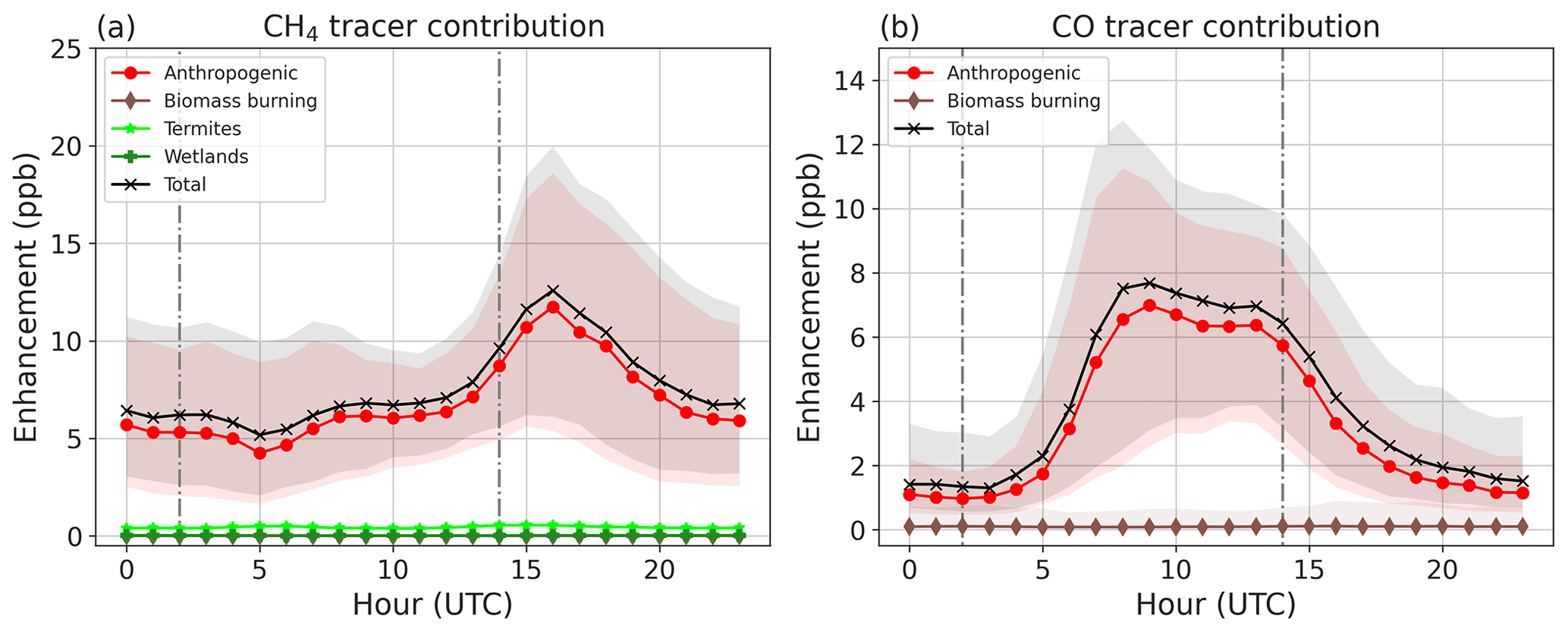
Figure 15Diurnal cycle of tracer contributions for (a) CH4 and (b) CO in situ surface concentration at MA.
4.3.3 XCH4
The model–data comparison for the NDACC data shows a very weak correlation (0.37) and a model underestimation of NDACC XCH4 (−5.65 ppb). This MBE has an opposite sign compared to TCCON CH4. Zhou et al. (2018) showed that NDACC XCH4 is generally about 10 ppb lower than TCCON XCH4 at Réunion Island due to their difference in vertical sensitivity. This pattern in the bias is the same as the one found by Ramonet et al. (2020) in comparisons of the CAMS reanalysis with NDACC and TCCON XCH4. Again, a seasonal pattern is found in the relative differences (Fig. 10b), which are caused by the reported bias for CH4 in the CAMS reanalysis data.
The tracer contributions to the XCH4 signal at MA in WRF-GHG are very similar to those at SDe, with seasonal enhancements from biomass burning and wetlands from Africa alongside a more constant anthropogenic part (Fig. 11b). Note that the contributions at MA seem to be slightly larger than those at SDe. This is because the atmospheric column above the high-altitude station of MA is smaller than the one above SDe and because the enhancements are transported from Africa and Madagascar by the westerlies higher up in the troposphere. The relative contributions averaged over the column are then higher at MA than at SDe.
4.3.4 Surface CO
WRF-GHG captures the in situ surface CO time series at MA quite well, and there is a high correlation of 0.83 (Table 3; Fig. 6e). The RMSE is about 11 ppb, and there is a small model overestimation of 5.51 ppb. During the day, a small anthropogenic enhancement is found (see Fig. 15b), as for CO2. As already noticed, thermal contrasts make air masses from the coastal areas arise during the day along the mountain slope before reaching the Maïdo Observatory. This air contains anthropogenic pollution. At the observatory itself, no anthropogenic CO fluxes are implemented, so the model is representing this daytime advection to some extent.
Another contributor is the BB signal from August to December. The contribution is not very visible in the diurnal cycle due to its seasonal nature, but daily enhancements of up to 40 ppb are simulated by WRF-GHG. BB contributions from the African continent and Madagascar are highest during the night, when MA is generally located in the free troposphere and transport from distant regions is detected (Baray et al., 2013).
4.3.5 XCO
A very high correlation (0.90) is found for the hourly averaged paired column data of NDACC and WRF-GHG (Table 3). In general, WRF-GHG slightly overestimates the observed XCO (MBE of 1.81 ppb). Note that the errors are larger (the overestimation is larger) for the TCCON data compared to the NDACC data (also Fig. 10b). This is probably linked to biases between the TCCON and NDACC data sets. Zhou et al. (2019) showed that there is a bias of 2.5 % between TCCON XCO and NDACC XCO at Réunion Island due to differences in the retrieval algorithm and data corrections.
As for XCH4, the average monthly tracer contributions of XCO at MA are very similar as those at SDe (Fig. 11b), with large contributions of BB emissions in the months August to December. Because of the unique location of MA, both the in situ observations and the column-averaged XCO are sensitive to these large seasonal events.
The above analysis was done using the WRF-GHG simulations from the innermost domain d03 (Fig. 2), which has a horizontal resolution of 2 × 2 km. As surface in situ observations are heavily influenced by local fluxes and dynamics, this high resolution is necessary to represent these measurements accurately, especially in regions with complex topography. As the ground-based remote sensing FTIR observations sample a much larger volume of air, a lower model resolution is likely sufficient to catch the fluxes and processes that influence them. Therefore, the model–data comparison for domains d01 and d02, with a horizontal resolution of 50 and 10 km, respectively, is given in this section. Table 4 gives the statistical metrics for the FTIR observations at both sites, for all model domains.
Table 4Overview of WRF-GHG performance of simulating hourly FTIR observations of GHG at Réunion Island, for all model domains. Comparison with the column observations is done using the smoothed model profiles.
The results are very similar among the different model resolutions, indicating that even a horizontal resolution of 50 km (as in d01) could be sufficient to simulate the FTIR observations at Réunion Island. In addition to the larger sampling volume, this can be explained by the fact that the most important contributions to the column are coming from remote areas such as Africa and Madagascar, situated in d01 and d02. The added value of high-resolution transport in d03 is negligible for the FTIR observations.
We studied the variability in CO2, CH4, and CO surface and column observations at Réunion Island and evaluated the possible factors influencing their observed mole fractions. This was achieved by comparing the available data sets with simulations of the WRF-GHG model over two periods between 2015 and 2017, totaling 20 months. The model performance was first evaluated for basic meteorological fields both near the surface and along atmospheric profiles. WRF-GHG shows good skill in reproducing these measurements, especially temperature. However, the local wind speed in Saint-Denis is overestimated by almost 4 m s−1, and also at Maïdo, there are some discrepancies in the wind speed and direction, which are likely linked to the complex topography and the model resolution of 2 km not being sufficient to represent the very local dynamical processes.
Nevertheless, the results enable us to answer the scientific questions posed in the introduction.
-
To what extent are the observations influenced by local and nearby sources and sinks or long-range transport of emitted gases?
At both Saint-Denis and Maïdo, the in situ observations are heavily influenced by local and nearby sources and sinks, especially for CO2. However, the in situ observations at Maïdo can detect both signals from the coastal regions and from afar at night, when the observatory is located in the boundary layer and the free troposphere, respectively. On the other hand, the column-averaged mole fractions describe different air masses to those near the surface and are not or only very slightly influenced by local activities. As shown by previous studies and confirmed here, these measurements at Réunion Island are influenced by processes from distant areas such as Africa and Madagascar. This is further evidenced by the fact that a model resolution of 50 km appears to be sufficient to simulate these observations. -
What are the different tracer contributions to the observed concentrations, both at the surface and in the total column?
The surface CO2 mole fractions in Saint-Denis follow a distinct diurnal cycle, with values up to 450 ppm at night, driven by local anthropogenic emissions, planetary boundary layer dynamics, and accumulation due to low wind speeds. Additionally, the signal includes respiration from vegetation that is carried by eastern winds from more rural regions. At the Maïdo Observatory, on the other hand, a similar diurnal cycle of CO2 is found but with much smaller amplitude. There, the surface CO2 mole fractions are essentially driven by the surrounding vegetation that take up CO2 during the day and release CO2 during the night through respiration. The different model tracers of XCO2 show contributions from fire emissions during the biomass burning season but also positive biogenic enhancements associated with the dry season. For CH4, tracer contributions reveal that the emission sources within the model domain have only a minimal effect on the overall signal. Besides the background, local anthropogenic fluxes are the major source influencing the in situ CH4 observations at Réunion Island. However, the comparisons between the model fields and observations at Saint-Denis show that the anthropogenic emissions from EDGAR are likely largely overestimated; this is even more evidenced at Maïdo. Some (minor) impacts from Africa and Madagascar can be seen in the XCH4 observations, with fire plumes during the biomass burning season and wetland emissions during the rainy season. For XCO, the importance of biomass burning plumes from Africa and elsewhere for the observed variability is confirmed. These plumes can also be detected by the in situ observations at Maïdo at night, while local anthropogenic signals are the main influence during the day. -
How accurate is WRF-GHG in simulating the different observation types of the three gases (CO2, CH4, and CO) in the Southern Indian Ocean region, in particular at Saint-Denis and at the Maïdo Observatory? What are its strengths and weaknesses?
In general, WRF-GHG shows great skill in simulating the different in situ surface and column observations of GHG. The simulations of XCO2 and XCO show a high correlation with the TCCON data, with coefficients of 0.9 and 0.89, respectively. Similarly, a Pearson correlation coefficient of 0.9 and low errors are found between the model and NDACC XCO time series. Furthermore, WRF-GHG is able to adequately reproduce the in situ CO observations at Maïdo, and consequently, to some extent, the anabatic winds that are typical for the northwestern part of the island, despite the differences in modeled and observed wind directions. The high model resolution of 2 km is needed to accurately represent local fluxes and small-scale processes that affect the in situ observations. However, because of the complex topography and the unique local wind patterns, an even higher resolution might be needed to simulate more precisely the observations at Maïdo. In addition, certain model flaws were discovered in this study. Due to an overestimation of local wind speeds in the capital, WRF-GHG underestimates the nocturnal CO2 buildup, leading to a correlation coefficient of only 0.62 between the model and surface CO2 measurements at Saint-Denis. Furthermore, we found a small model underestimation of the amplitude of the diurnal cycle of surface CO2 at Maïdo, which might indicate that the VPRM parameters could be improved for this region. Finally, WRF-GHG fails to accurately reproduce the different CH4 observations at Réunion Island due to a seasonal bias in the background arising from the CAMS reanalysis.
This study showed an application of the WRF-GHG model in a region of the globe where it had not yet been run before. It demonstrated that WRF-GHG had great skill in simulating the meteorological fields and different in situ surface and column observations of GHG. However, the results are highly dependent on accurate boundary conditions and the availability of high-resolution emission inventories.
As mentioned in Sect. 3.1, this study uses the VPRM parameter set that was optimized by Botía et al. (2021) for the Amazon region in Brazil. Table A1 gives the exact values for every vegetation class.
A smoothing correction is applied when comparing the model data with the TCCON and NDACC data. Retrieved column-averaged mole fractions are affected by the observing system characteristics, and therefore, Rodgers and Connor (2003) suggest taking into account the a priori information and averaging kernels of the retrieval when calculating the Xgas of the model. The different steps undertaken to calculate this are explained hereafter for TCCON and NDACC separately.
Generally, the smoothed Xgas from WRF-GHG is calculated as follows:
where is the partial column number density of dry air in layer i, and is the volume mixing ratio with respect to dry air in layer i of the smoothed model profile. In the following, all parameters indicating a volume mixing ratio or column number density are also with respect to dry air; however, for brevity, it will not be specified any more.
B1 TCCON
Equation (B1) requires a smoothed vertical profile (). Since TCCON does not provide profile retrievals, we cannot calculate this. Instead, we use the following smoothing equation for TCCON:
where TCTCCON is the total column (number density) of dry air from TCCON (for an atmospheric column up to 50 hPa). Similarly, is the total column of the a priori mole fraction from TCCON calculated as the sum of the partial columns over those layers i that are below 50 hPa. Furthermore, a is the vector with the column averaging kernels of TCCON.
The regridded partial column profile of WRF-GHG () and the total column of dry air from WRF (TCWRF,regrid) are calculated in a few steps which are explained below. By including the total column of dry air from WRF in Eq. (B2), we want to eliminate potential differences in air between TCCON and the model. As such, the priority is given to the volume mixing ratio profiles (instead of the calculation of dry air). The steps we take are as follows:
-
Extend the WRF-GHG atmospheric profiles (gas mole fraction, pressure, temperature, and water vapor) above the model limit (50 hPa) using information of the TCCON a priori profiles.
-
Calculate the dry air partial column in layer i using the ideal gas law as follows:
with P as atmospheric pressure, T as air temperature, R as the ideal gas constant, q as the mass mixing ratio of water vapor, and τ as the layer thickness.
-
Calculate the gas number density partial columns as , with as the gas mole fraction in layer i.
-
Regrid these partial column profiles to the full TCCON grid using a transformation matrix D, as in Langerock et al. (2015), as follows:
and
-
Finish with , where the sum is taken over all layers i below 50 hPa.
B2 NDACC
The smoothed Xgas from WRF-GHG at MA is calculated slightly differently to at SDe, as, for NDACC, the volume mixing ratio profiles are provided. The smoothing equation can be written as follows:
where is the volume mixing ratio (VMR) a priori profile from NDACC, and A is the NDACC VMR averaging kernel matrix. Similar to that for TCCON, a few steps need to be taken to make the WRF-GHG data fit in Eq. (B3). Steps 1–4, as described above, should be followed but by using NDACC information instead of TCCON (a priori VMR profile, temperature, and water vapor profiles; vertical grid). Then the regridded VMR profile from WRF-GHG is calculated as . Finally, the smoothed dry air mole fraction at MA is given by the following:
where the sum is taken over all layers i below 50 hPa.
The full time series of both the observed and modeled concentrations at SDe and MA are given in the figures hereafter. Figures C1 and C2 show the time series of the in situ data at SDe and MA, respectively. Similarly, Figs. C3 and C4 show the comparison of the FTIR data at SDe (TCCON) and MA (NDACC).
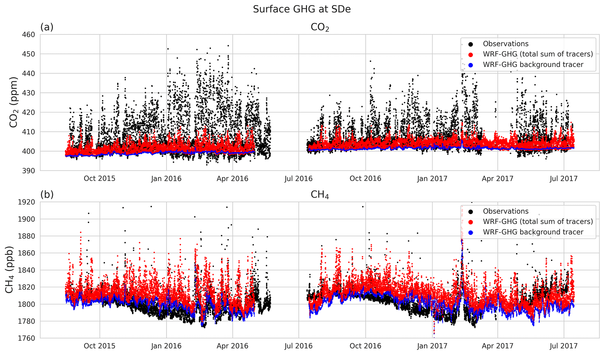
Figure C1Time series of all observed (black) and modeled (red) in situ concentrations at SDe of (a) CO2 and (b) CH4. The blue dots represent the modeled background tracer.
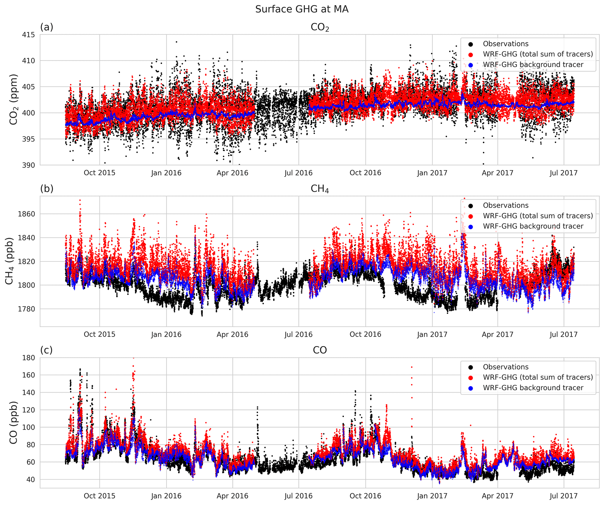
Figure C2Time series of all observed (black) and modeled (red) in situ concentrations at MA of (a) CO2, (b) CH4, and (c) CO. The blue dots represent the modeled background tracer.
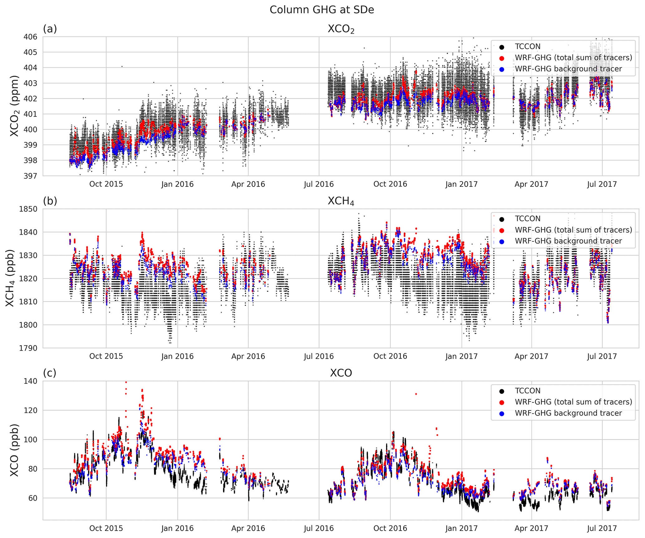
Figure C3Time series of all observed (black) and modeled (red) column concentrations at SDe of (a) CO2, (b) CH4, and (c) CO. The blue dots represent the modeled background tracer. The modeled data are hourly and smoothed. The observed data are scaled to the atmospheric column until 50 hPa, and all available measurements are shown.
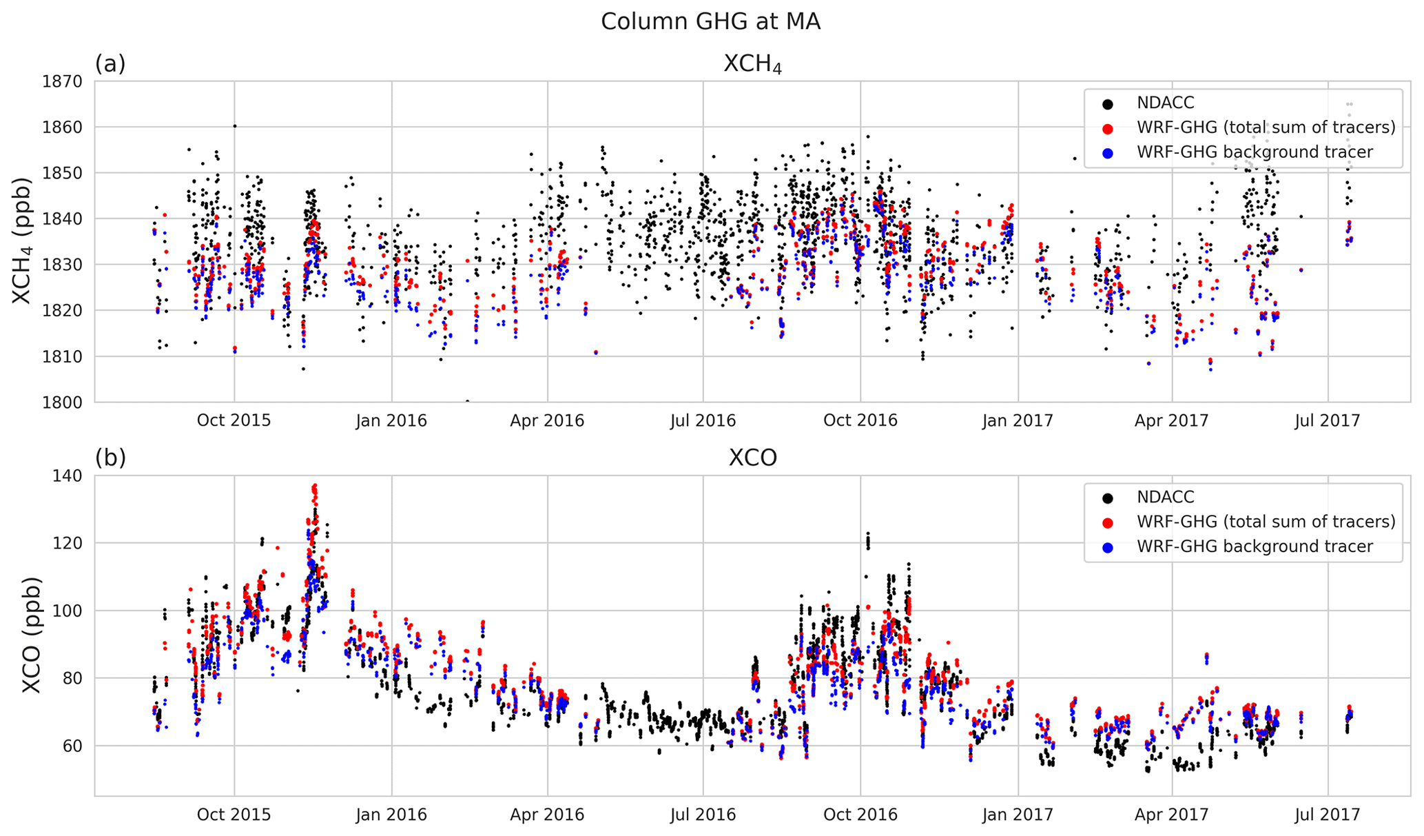
Figure C4Time series of all observed (black) and modeled (red) column concentrations at MA of (a) CH4 and (b) CO. The blue dots represent the modeled background tracer. The modeled data are hourly and smoothed. The observed data are scaled to atmospheric column until 50 hPa, and all available measurements are shown.
The data used in this publication were obtained from Martine De Mazière, as part of the Network for the Detection of Atmospheric Composition Change (NDACC), and are available through the NDACC website https://www-air.larc.nasa.gov/missions/ndacc/data.html?station=la.reunion.maido/hdf/ftir/ (De Mazière, 2019). The TCCON data were obtained from the TCCON Data Archive hosted by CaltechDATA at https://doi.org/10.14291/TCCON.GGG2014.REUNION01.R1 (De Mazière et al., 2017). The ICOS data used for this study are hosted on the Carbon Portal at https://doi.org/10.18160/Z7WE-5XHP (De Mazière et al., 2021). The ERA5 and CAMS reanalysis data set (https://doi.org/10.24381/cds.adbb2d47, Hersbach et al., 2018a; https://doi.org/10.24381/cds.bd0915c6, Hersbach et al., 2018b), used as input for the WRF-GHG simulations, was downloaded from the Copernicus Climate Change Service (C3S) Climate Data Store (2021). The WRF-Chem model code is distributed by NCAR (https://doi.org/10.5065/D6MK6B4K, NCAR, 2020).
SC set up the model simulations, did the analysis, and wrote the paper. JB provided the anthropogenic CO fluxes at Réunion Island and its description. VD provided the meteorological radiosonde profiles. BL provided expertise on the FTIR data and model comparison techniques. DF assisted in setting up the model and, together with JFM, helped with correctly interpreting the results. JMM, CH, NK, MR, and ML provided the FTIR and in situ measurements on Réunion Island. EM and MDM provided general guidance and support during the analysis and revised and edited the paper. All authors reviewed and commented on the paper.
The contact author has declared that neither they nor their co-authors have any competing interests.
The results contain modified Copernicus Atmosphere Monitoring Service information 2020–2021. Neither the European Commission nor ECMWF is responsible for any use that may be made of the Copernicus information or data it contains.
Publisher's note: Copernicus Publications remains neutral with regard to jurisdictional claims in published maps and institutional affiliations.
We acknowledge the providers of the observational data sets.
The authors also acknowledge the European Communities, the Région Réunion Island, CNRS, and Université de la Réunion Island, for their support and contribution in the construction phase of the research infrastructure OPAR (Observatoire de Physique de l'Atmosphère à La Réunion). OPAR is presently funded by CNRS (INSU), Météo-France, and Université de La Réunion and managed by OSU-R (Observatoire des Sciences de l'Univers à La Réunion, UAR 3365). OPAR is supported by the French research infrastructure ACTRIS-FR (Aerosols, Clouds, and Trace gases Research InfraStructure – France).
We thank Christophe Gerbig, Roberto Kretschmer, and Thomas Koch (MPI BGC), for their work on the VPRM preprocessor and support on installing the software at the BIRA-IASB servers. The authors also wish to thank Julia Marshall (DLR) and Michael Gałkowski (MPI BGC), for their guidance in running the WRF-GHG model and interpreting its results. Additionally, we thank the broader WRF-GHG community, for the regular exchange of expertise. Finally, we thank Mahesh Kumar Sha (BIRA-IASB) and Minqiang Zhou (IAP, CAS), for the helpful discussions on the interpretation of the data.
This research has been supported by the Belgian Federal Government through the tax exemption law for promoting scientific research (Art. 275/3 of CIR92).
This paper was edited by Christoph Gerbig and reviewed by two anonymous referees.
Ahmadov, R., Gerbig, C., Kretschmer, R., Koerner, S., Neininger, B., Dolman, A. J., and Sarrat, C.: Mesoscale covariance of transport and CO2 fluxes: Evidence from observations and simulations using the WRF-VPRM coupled atmosphere-biosphere model, J. Geophys. Res.-Atmos., 112, D22107, https://doi.org/10.1029/2007JD008552, 2007. a, b
Baldy, S., Ancellet, G., Bessafi, M., Badr, A., and Luk, D. L. S.: Field observations of the vertical distribution of tropospheric ozone at the island of Reunion (southern tropics), J. Geophys. Res.-Atmos., 101, 23835–23849, https://doi.org/10.1029/95JD02929, 1996. a, b, c
Baray, J.-L., Courcoux, Y., Keckhut, P., Portafaix, T., Tulet, P., Cammas, J.-P., Hauchecorne, A., Godin Beekmann, S., De Mazière, M., Hermans, C., Desmet, F., Sellegri, K., Colomb, A., Ramonet, M., Sciare, J., Vuillemin, C., Hoareau, C., Dionisi, D., Duflot, V., Vérèmes, H., Porteneuve, J., Gabarrot, F., Gaudo, T., Metzger, J.-M., Payen, G., Leclair de Bellevue, J., Barthe, C., Posny, F., Ricaud, P., Abchiche, A., and Delmas, R.: Maïdo observatory: a new high-altitude station facility at Reunion Island (21∘ S, 55∘ E) for long-term atmospheric remote sensing and in situ measurements, Atmos. Meas. Tech., 6, 2865–2877, https://doi.org/10.5194/amt-6-2865-2013, 2013. a, b, c, d, e, f
Barlage, M., Miao, S., and Chen, F.: Impact of physics parameterizations on high-resolution weather prediction over two Chinese megacities, J. Geophys. Res.-Atmos., 121, 4487–4498, https://doi.org/10.1002/2015JD024450, 2016. a
Beck, V., Koch, T., Kretschmer, R., Ahmadov, R., Gerbig, C., Marshall, J., Pillai, D., and Heimann, M.: The WRF Greenhouse Gas Model (WRF-GHG), Technical Report No. 25, techreport 25, Max Planck Institute for Biogeochemistry, https://www.bgc-jena.mpg.de/bgc-systems/pmwiki2/uploads/Download/Wrf-ghg/WRF-GHG_Techn_Report.pdf (last access: 27 September 2018), 2011. a
Beck, V., Gerbig, C., Koch, T., Bela, M. M., Longo, K. M., Freitas, S. R., Kaplan, J. O., Prigent, C., Bergamaschi, P., and Heimann, M.: WRF-Chem simulations in the Amazon region during wet and dry season transitions: evaluation of methane models and wetland inundation maps, Atmos. Chem. Phys., 13, 7961–7982, https://doi.org/10.5194/acp-13-7961-2013, 2013. a, b
Bloom, A. A., Bowman, K. W., Lee, M., Turner, A. J., Schroeder, R., Worden, J. R., Weidner, R., McDonald, K. C., and Jacob, D. J.: A global wetland methane emissions and uncertainty dataset for atmospheric chemical transport models (WetCHARTs version 1.0), Geosci. Model Dev., 10, 2141–2156, https://doi.org/10.5194/gmd-10-2141-2017, 2017. a
Borsdorff, T., aan de Brugh, J., Pandey, S., Hasekamp, O., Aben, I., Houweling, S., and Landgraf, J.: Carbon monoxide air pollution on sub-city scales and along arterial roads detected by the Tropospheric Monitoring Instrument, Atmos. Chem. Phys., 19, 3579–3588, https://doi.org/10.5194/acp-19-3579-2019, 2019. a
Botía, S., Komiya, S., Marshall, J., Koch, T., Gałkowski, M., Lavric, J., Gomes-Alves, E., Walter, D., Fisch, G., Pinho, D. M., Nelson, B. W., Martins, G., Luijkx, I. T., Koren, G., Florentie, L., Carioca de Araújo, A., Sá, M., Andreae, M. O., Heimann, M., Peters, W., and Gerbig, C.: The CO2 record at the Amazon Tall Tower Observatory: A new opportunity to study processes on seasonal and inter-annual scales, Glob. Change Biol., 28, 588–611, https://doi.org/10.1111/gcb.15905, 2021. a, b
Bretherton, C. S. and Park, S.: A New Moist Turbulence Parameterization in the Community Atmosphere Model, J. Climate, 22, 3422–3448, https://doi.org/10.1175/2008JCLI2556.1, 2009. a
Brioude, J., Petron, G., Frost, G., Ahmadov, R., M. Angevine, W., Hsie, E.-Y., Kim, S.-W., Lee, S.-H., McKeen, S., Trainer, M., Fehsenfeld, F., Holloway, J., Peischl, J., B. Ryerson, T., and Gurney, K.: A new inversion method to calculate emission inventories without a prior at mesoscale: Application to the anthropogenic CO2 emission from Houston, Texas, J. Geophys. Res., 117, D05312, https://doi.org/10.1029/2011JD016918, 2012. a
Brioude, J., Angevine, W. M., Ahmadov, R., Kim, S.-W., Evan, S., McKeen, S. A., Hsie, E.-Y., Frost, G. J., Neuman, J. A., Pollack, I. B., Peischl, J., Ryerson, T. B., Holloway, J., Brown, S. S., Nowak, J. B., Roberts, J. M., Wofsy, S. C., Santoni, G. W., Oda, T., and Trainer, M.: Top-down estimate of surface flux in the Los Angeles Basin using a mesoscale inverse modeling technique: assessing anthropogenic emissions of CO, NOx and CO2 and their impacts, Atmos. Chem. Phys., 13, 3661–3677, https://doi.org/10.5194/acp-13-3661-2013, 2013. a
Crippa, M., Guizzardi, D., Muntean, M., and Schaaf, E.: EDGAR v5.0 Global Air Pollutant Emissions, European Commission, Joint Research Centre (JRC) [data set], http://data.europa.eu/89h/377801af-b094-4943-8fdc-f79a7c0c2d19 (last access: 2 April 2020), 2019a. a
Crippa, M., Guizzardi, D., Muntean, M., Schaaf, E., Lo Vullo, E., Solazzo, E., Monforti-Ferrario, F., Olivier, J., and Vignati, E.: EDGAR v5.0 Greenhouse Gas Emissions, European Commission, Joint Research Centre (JRC) [data set], http://data.europa.eu/89h/488dc3de-f072-4810-ab83-47185158ce2a (last access: 7 April 2021), 2019b. a
Dayalu, A., Munger, J. W., Wang, Y., Wofsy, S. C., Zhao, Y., Nehrkorn, T., Nielsen, C., McElroy, M. B., and Chang, R.: Carbon dioxide emissions in Northern China based on atmospheric observations from 2005 to 2009, Atmos. Chem. Phys. Discuss. [preprint], https://doi.org/10.5194/acp-2018-632, 2018. a
Dekker, I. N., Houweling, S., Aben, I., Röckmann, T., Krol, M., Martínez-Alonso, S., Deeter, M. N., and Worden, H. M.: Quantification of CO emissions from the city of Madrid using MOPITT satellite retrievals and WRF simulations, Atmos. Chem. Phys., 17, 14675–14694, https://doi.org/10.5194/acp-17-14675-2017, 2017. a
Dekker, I. N., Houweling, S., Pandey, S., Krol, M., Röckmann, T., Borsdorff, T., Landgraf, J., and Aben, I.: What caused the extreme CO concentrations during the 2017 high-pollution episode in India?, Atmos. Chem. Phys., 19, 3433–3445, https://doi.org/10.5194/acp-19-3433-2019, 2019. a
De Mazière, M.: M. De Mazière (IASB-BIRA) – Bruker 125HR installed in March 2013 for NDACC measurements, NDACC [data set], https://www-air.larc.nasa.gov/missions/ndacc/data.html?station=la.reunion.maido/hdf/ftir/, last access: 7 May 2019. a
De Mazière, M., Sha, M. K., Desmet, F., Hermans, C., Scolas, F., Kumps, N., Metzger, J.-M., Duflot, V., and Cammas, J.-P.: TCCON data from Réunion Island (RE), Release GGG2014.R1 (Version R1), CaltechDATA [data set], https://doi.org/10.14291/TCCON.GGG2014.REUNION01.R1, 2017. a, b
De Mazière, M., Thompson, A. M., Kurylo, M. J., Wild, J. D., Bernhard, G., Blumenstock, T., Braathen, G. O., Hannigan, J. W., Lambert, J.-C., Leblanc, T., McGee, T. J., Nedoluha, G., Petropavlovskikh, I., Seckmeyer, G., Simon, P. C., Steinbrecht, W., and Strahan, S. E.: The Network for the Detection of Atmospheric Composition Change (NDACC): history, status and perspectives, Atmos. Chem. Phys., 18, 4935–4964, https://doi.org/10.5194/acp-18-4935-2018, 2018. a
De Mazière, M., Sha, M. K., Ramonet, M., and ICOS RI: ICOS Atmosphere Level 2 data, La Réunion, release 2021-1 (Version 1.0). ICOS ERIC – Carbon Portal [data set], https://doi.org/10.18160/Z7WE-5XHP, 2021. a, b
Dominutti, P. A., Renard, P., Vaïtilingom, M., Bianco, A., Baray, J.-L., Borbon, A., Bourianne, T., Burnet, F., Colomb, A., Delort, A.-M., Duflot, V., Houdier, S., Jaffrezo, J.-L., Joly, M., Leremboure, M., Metzger, J.-M., Pichon, J.-M., Ribeiro, M., Rocco, M., Tulet, P., Vella, A., Leriche, M., and Deguillaume, L.: Insights into tropical cloud chemistry in Réunion (Indian Ocean): results from the BIO-MAÏDO campaign, Atmos. Chem. Phys., 22, 505–533, https://doi.org/10.5194/acp-22-505-2022, 2022. a
Duflot, V., Dils, B., Baray, J. L., De Mazière, M., Attié, J. L., Vanhaelewyn, G., Senten, C., Vigouroux, C., Clain, G., and Delmas, R.: Analysis of the origin of the distribution of CO in the subtropical southern Indian Ocean in 2007, J. Geophys. Res.-Atmos., 115, D22106, https://doi.org/10.1029/2010JD013994, 2010. a, b, c, d
Duflot, V., Tulet, P., Flores, O., Barthe, C., Colomb, A., Deguillaume, L., Vaïtilingom, M., Perring, A., Huffman, A., Hernandez, M. T., Sellegri, K., Robinson, E., O'Connor, D. J., Gomez, O. M., Burnet, F., Bourrianne, T., Strasberg, D., Rocco, M., Bertram, A. K., Chazette, P., Totems, J., Fournel, J., Stamenoff, P., Metzger, J.-M., Chabasset, M., Rousseau, C., Bourrianne, E., Sancelme, M., Delort, A.-M., Wegener, R. E., Chou, C., and Elizondo, P.: Preliminary results from the FARCE 2015 campaign: multidisciplinary study of the forest–gas–aerosol–cloud system on the tropical island of La Réunion, Atmos. Chem. Phys., 19, 10591–10618, https://doi.org/10.5194/acp-19-10591-2019, 2019. a, b, c, d
Dupont, J.-C., Haeffelin, M., Badosa, J., Clain, G., Raux, C., and Vignelles, D.: Characterization and Corrections of Relative Humidity Measurement from Meteomodem M10 Radiosondes at Midlatitude Stations, J. Atmos. Ocean. Tech., 37, 857–871, https://doi.org/10.1175/JTECH-D-18-0205.1, 2020. a
Errera, Q., Bennouna, Y., Schulz, M., Eskes, H., Basart, S., Benedictow, A., Blechschmidt, A.-M., Chabrillat, S., Clark, H., Cuevas, E., Flentje, H., Hansen, K., U. Im, J. K., Langerock, B., Petersen, K., Richter, A., Sudarchikova, N., Thouret, V., Wagner, A., Wang, Y., Warneke, T., and Zerefos, C.: Validation report of the CAMS global Reanalysis of aerosols and reactive gases, years 2003–2020, Tech. rep., Copernicus Atmosphere Monitoring Service (CAMS), https://doi.org/10.24380/8gf9-k005, 2021. a, b
Feng, S., Lauvaux, T., Newman, S., Rao, P., Ahmadov, R., Deng, A., Díaz-Isaac, L. I., Duren, R. M., Fischer, M. L., Gerbig, C., Gurney, K. R., Huang, J., Jeong, S., Li, Z., Miller, C. E., O'Keeffe, D., Patarasuk, R., Sander, S. P., Song, Y., Wong, K. W., and Yung, Y. L.: Los Angeles megacity: a high-resolution land–atmosphere modelling system for urban CO2 emissions, Atmos. Chem. Phys., 16, 9019–9045, https://doi.org/10.5194/acp-16-9019-2016, 2016. a, b
Foucart, B., Sellegri, K., Tulet, P., Rose, C., Metzger, J.-M., and Picard, D.: High occurrence of new particle formation events at the Maïdo high-altitude observatory (2150 m), Réunion (Indian Ocean), Atmos. Chem. Phys., 18, 9243–9261, https://doi.org/10.5194/acp-18-9243-2018, 2018. a, b, c, d, e, f
Frey, M. M., Hase, F., Blumenstock, T., Dubravica, D., Groß, J., Göttsche, F., Handjaba, M., Amadhila, P., Mushi, R., Morino, I., Shiomi, K., Sha, M. K., de Mazière, M., and Pollard, D. F.: Long-term column-averaged greenhouse gas observations using a COCCON spectrometer at the high-surface-albedo site in Gobabeb, Namibia, Atmos. Meas. Tech., 14, 5887–5911, https://doi.org/10.5194/amt-14-5887-2021, 2021. a
García, M. Á., Sánchez, M. L., and Pérez, I. A.: Differences between carbon dioxide levels over suburban and rural sites in Northern Spain, Environm. Sci. Pollut. R., 19, 432–439, https://doi.org/10.1007/s11356-011-0575-4, 2012. a
Giglio, L., Csiszar, I., and Justice, C. O.: Global distribution and seasonality of active fires as observed with the Terra and Aqua Moderate Resolution Imaging Spectroradiometer (MODIS) sensors, J. Geophys. Res.-Biogeo., 111, G02016, https://doi.org/10.1029/2005JG000142, 2006. a
Grell, G. A. and Freitas, S. R.: A scale and aerosol aware stochastic convective parameterization for weather and air quality modeling, Atmos. Chem. Phys., 14, 5233–5250, https://doi.org/10.5194/acp-14-5233-2014, 2014. a
Guilpart, E., Vimeux, F., Evan, S., Brioude, J., Metzger, J.-M., Barthe, C., Risi, C., and Cattani, O.: The isotopic composition of near-surface water vapor at the Maïdo observatory (Reunion Island, southwestern Indian Ocean) documents the controls of the humidity of the subtropical troposphere, J. Geophys. Res.-Atmos., 122, 9628–9650, https://doi.org/10.1002/2017JD026791, 2017. a, b, c
Hase, F., Frey, M., Blumenstock, T., Groß, J., Kiel, M., Kohlhepp, R., Mengistu Tsidu, G., Schäfer, K., Sha, M. K., and Orphal, J.: Application of portable FTIR spectrometers for detecting greenhouse gas emissions of the major city Berlin, Atmos. Meas. Tech., 8, 3059–3068, https://doi.org/10.5194/amt-8-3059-2015, 2015. a
Hersbach, H., Bell, B., Berrisford, P., Biavati, G., Horányi, A., Muñoz Sabater, J., Nicolas, J., Peubey, C., Radu, R., Rozum, I., Schepers, D., Simmons, A., Soci, C., Dee, D., and Thépaut, J.-N.: ERA5 hourly data on single levels from 1979 to present, Copernicus Climate Change Service (C3S) Climate Data Store (CDS) [data set], https://doi.org/10.24381/cds.adbb2d47, 2018a. a, b
Hersbach, H., Bell, B., Berrisford, P., Biavati, G., Horányi, A., Muñoz Sabater, J., Nicolas, J., Peubey, C., Radu, R., Rozum, I., Schepers, D., Simmons, A., Soci, C., Dee, D., and Thépaut, J.-N.: ERA5 hourly data on pressure levels from 1979 to present, Copernicus Climate Change Service (C3S) Climate Data Store (CDS) [data set], https://doi.org/10.24381/cds.bd0915c6, 2018b. a, b
Hu, X.-M., Crowell, S., Wang, Q., Zhang, Y., Davis, K. J., Xue, M., Xiao, X., Moore, B., Wu, X., Choi, Y., and DiGangi, J. P.: Dynamical Downscaling of CO2 in 2016 Over the Contiguous United States Using WRF-VPRM, a Weather-Biosphere-Online-Coupled Model, J. Adv. Model. Earth Syst., 12, e2019MS001875, https://doi.org/10.1029/2019MS001875, 2020. a
Iacono, M. J., Delamere, J. S., Mlawer, E. J., Shephard, M. W., Clough, S. A., and Collins, W. D.: Radiative forcing by long-lived greenhouse gases: Calculations with the AER radiative transfer models, J. Geophys. Res.-Atmos., 113, D13103, https://doi.org/10.1029/2008JD009944, 2008. a
Idso, S. B., Idso, C. D., and Balling, R. C.: Seasonal and diurnal variations of near-surface atmospheric CO2 concentration within a residential sector of the urban CO2 dome of Phoenix, AZ, USA, Atmos. Environ., 36, 1655–1660, https://doi.org/10.1016/S1352-2310(02)00159-0, 2002. a, b
Inness, A., Ades, M., Agustí-Panareda, A., Barré, J., Benedictow, A., Blechschmidt, A.-M., Dominguez, J. J., Engelen, R., Eskes, H., Flemming, J., Huijnen, V., Jones, L., Kipling, Z., Massart, S., Parrington, M., Peuch, V.-H., Razinger, M., Remy, S., Schulz, M., and Suttie, M.: The CAMS reanalysis of atmospheric composition, Atmos. Chem. Phys., 19, 3515–3556, https://doi.org/10.5194/acp-19-3515-2019, 2019. a
IPCC: Summary for Policymakers, in: Climate Change 2021: The Physical Science Basis. Contribution of Working Group I to the Sixth Assessment Report of the Intergovernmental Panel on Climate Change, edited by: Masson-Delmotte, V., Zhai, P., Pirani, A., Connors, S. L., Péan, C., Berger, S., Caud, N., Chen, Y., Goldfarb, L., Gomis, M. I., Huang, M., Leitzell, K., Lonnoy, E., Matthews, J. B. R., Maycock, T. K., Waterfield, T., Yelekçi, O., Yu, R., and Zhou, B., Cambridge University Press, Cambridge, United Kingdom and New York, NY, USA, 3–32, https://doi.org/10.1017/9781009157896.001, 2021. a
Jamroensan, A.: Improving bottom-up and top-down estimates of carbon fluxes in the Midwestern USA, PhD thesis, University of Iowa, https://doi.org/10.17077/etd.99sd8cdc, 2013. a
Janjić, Z. I.: The Step-Mountain Eta Coordinate Model: Further Developments of the Convection, Viscous Sublayer, and Turbulence Closure Schemes, Mon. Weather Rev., 122, 927–945, https://doi.org/10.1175/1520-0493(1994)122<0927:TSMECM>2.0.CO;2, 1994. a
Jung, M., Henkel, K., Herold, M., and Churkina, G.: Exploiting synergies of global land cover products for carbon cycle modeling, Remote Sens. Environ., 101, 534–553, https://doi.org/10.1016/j.rse.2006.01.020, 2006. a
Kim, Y., Sartelet, K., Raut, J.-C., and Chazette, P.: Evaluation of the Weather Research and Forecast/Urban Model Over Greater Paris, Bound.-Lay. Meteorol., 149, 1573–1472, https://doi.org/10.1007/s10546-013-9838-6, 2013. a
Lac, C., Chaboureau, J.-P., Masson, V., Pinty, J.-P., Tulet, P., Escobar, J., Leriche, M., Barthe, C., Aouizerats, B., Augros, C., Aumond, P., Auguste, F., Bechtold, P., Berthet, S., Bielli, S., Bosseur, F., Caumont, O., Cohard, J.-M., Colin, J., Couvreux, F., Cuxart, J., Delautier, G., Dauhut, T., Ducrocq, V., Filippi, J.-B., Gazen, D., Geoffroy, O., Gheusi, F., Honnert, R., Lafore, J.-P., Lebeaupin Brossier, C., Libois, Q., Lunet, T., Mari, C., Maric, T., Mascart, P., Mogé, M., Molinié, G., Nuissier, O., Pantillon, F., Peyrillé, P., Pergaud, J., Perraud, E., Pianezze, J., Redelsperger, J.-L., Ricard, D., Richard, E., Riette, S., Rodier, Q., Schoetter, R., Seyfried, L., Stein, J., Suhre, K., Taufour, M., Thouron, O., Turner, S., Verrelle, A., Vié, B., Visentin, F., Vionnet, V., and Wautelet, P.: Overview of the Meso-NH model version 5.4 and its applications, Geosci. Model Dev., 11, 1929–1969, https://doi.org/10.5194/gmd-11-1929-2018, 2018. a
Landschützer, P., Gruber, N., and Bakker, D. C. E.: An observation-based global monthly gridded sea surface pCO2 product from 1982 onward and its monthly climatology (NCEI Accession 0160558), NOAA National Centers for Environmental Information [data set], https://doi.org/10.7289/v5z899n6, 2017. a
Langerock, B., De Mazière, M., Hendrick, F., Vigouroux, C., Desmet, F., Dils, B., and Niemeijer, S.: Description of algorithms for co-locating and comparing gridded model data with remote-sensing observations, Geosci. Model Dev., 8, 911–921, https://doi.org/10.5194/gmd-8-911-2015, 2015. a
Lesouëf, D., Gheusi, F., Delmas, R., and Escobar, J.: Numerical simulations of local circulations and pollution transport over Reunion Island, Ann. Geophys., 29, 53–69, https://doi.org/10.5194/angeo-29-53-2011, 2011. a, b, c, d
Lesouëf, D., Gheusi, F., Chazette, P., Delmas, R., and Sanak, J.: Low Tropospheric Layers Over Reunion Island in Lidar-Derived Observations and a High-Resolution Model, Bound.-Lay. Meteorol., 149, 425–453, https://doi.org/10.1007/s10546-013-9851-9, 2013. a
Li, X., Hu, X.-M., Cai, C., Jia, Q., Zhang, Y., Liu, J., Xue, M., Xu, J., Wen, R., and Crowell, S. M. R.: Terrestrial CO2 Fluxes, Concentrations, Sources and Budget in Northeast China: Observational and Modeling Studies, J. Geophys. Res.-Atmos., 125, e2019JD031686, https://doi.org/10.1029/2019JD031686, 2020. a
Liu, Y., Yue, T., Zhang, L., Zhao, N., Zhao, M., and Liu, Y.: Simulation and analysis of XCO2 in North China based on high accuracy surface modeling, Environ. Sci. Pollut. R., 25, 27378–27392, https://doi.org/10.1007/s11356-018-2683-x, 2018. a
Lunt, M. F., Palmer, P. I., Feng, L., Taylor, C. M., Boesch, H., and Parker, R. J.: An increase in methane emissions from tropical Africa between 2010 and 2016 inferred from satellite data, Atmos. Chem. Phys., 19, 14721–14740, https://doi.org/10.5194/acp-19-14721-2019, 2019. a
Mahadevan, P., Wofsy, S. C., Matross, D. M., Xiao, X., Dunn, A. L., Lin, J. C., Gerbig, C., Munger, J. W., Chow, V. Y., and Gottlieb, E. W.: A satellite-based biosphere parameterization for net ecosystem CO2 exchange: Vegetation Photosynthesis and Respiration Model (VPRM), Global Biogeochem. Cy., 22, GB2005, https://doi.org/10.1029/2006GB002735, 2008. a, b, c
Makarova, M. V., Alberti, C., Ionov, D. V., Hase, F., Foka, S. C., Blumenstock, T., Warneke, T., Virolainen, Y. A., Kostsov, V. S., Frey, M., Poberovskii, A. V., Timofeyev, Y. M., Paramonova, N. N., Volkova, K. A., Zaitsev, N. A., Biryukov, E. Y., Osipov, S. I., Makarov, B. K., Polyakov, A. V., Ivakhov, V. M., Imhasin, H. Kh., and Mikhailov, E. F.: Emission Monitoring Mobile Experiment (EMME): an overview and first results of the St. Petersburg megacity campaign 2019, Atmos. Meas. Tech., 14, 1047–1073, https://doi.org/10.5194/amt-14-1047-2021, 2021. a
Massen, F. and Beck, E.-G.: Accurate Estimation of CO2 Background Level from Near Ground Measurements at Non-Mixed Environments, Springer Berlin Heidelberg, Berlin, Heidelberg, https://doi.org/10.1007/978-3-642-14776-0_31, 2011. a
Morrison, H., Thompson, G., and Tatarskii, V.: Impact of Cloud Microphysics on the Development of Trailing Stratiform Precipitation in a Simulated Squall Line: Comparison of One- and Two-Moment Schemes, Mon. Weather Rev., 137, 991–1007, https://doi.org/10.1175/2008MWR2556.1, 2009. a
Nassar, R., Napier-Linton, L., Gurney, K. R., Andres, R. J., Oda, T., Vogel, F. R., and Deng, F.: Improving the temporal and spatial distribution of CO2 emissions from global fossil fuel emission data sets, J. Geophys. Res.-Atmos., 118, 917–933, https://doi.org/10.1029/2012JD018196, 2013. a, b
National Center for Atmospheric Research (NCAR): Weather Research and Forecasting Model Version 4.1.5, NCAR [code], https://doi.org/10.5065/D6MK6B4K, 2020. a
Oda, T. and Maksyutov, S.: A very high-resolution (1 km × 1 km) global fossil fuel CO2 emission inventory derived using a point source database and satellite observations of nighttime lights, Atmos. Chem. Phys., 11, 543–556, https://doi.org/10.5194/acp-11-543-2011, 2011. a
Oda, T. and Maksyuto, S.: ODIAC Fossil Fuel CO2 Emissions Dataset (ODIAC2020), Center for Global Environmental Research, National Institute for Environmental Studies [data set], https://doi.org/10.17595/20170411.001, 2015. a
Oda, T., Maksyutov, S., and Andres, R. J.: The Open-source Data Inventory for Anthropogenic CO2, version 2016 (ODIAC2016): a global monthly fossil fuel CO2 gridded emissions data product for tracer transport simulations and surface flux inversions, Earth Syst. Sci. Data, 10, 87–107, https://doi.org/10.5194/essd-10-87-2018, 2018. a
Park, C., Gerbig, C., Newman, S., Ahmadov, R., Feng, S., Gurney, K. R., Carmichael, G. R., Park, S.-Y., Lee, H.-W., Goulden, M., Stutz, J., Peischl, J., and Ryerson, T.: CO2 Transport, Variability, and Budget over the Southern California Air Basin Using the High-Resolution WRF-VPRM Model during the CalNex 2010 Campaign, J. Appl. Meteorol. Clim., 57, 1337–1352, https://doi.org/10.1175/JAMC-D-17-0358.1, 2018. a
Park, C., Park, S.-Y., Gurney, K. R., Gerbig, C., DiGangi, J. P., Choi, Y., and Lee, H. W.: Numerical simulation of atmospheric CO2 concentration and flux over the Korean Peninsula using WRF-VPRM model during Korus-AQ 2016 campaign, PLoS ONE, 15, 1–21, https://doi.org/10.1371/journal.pone.0228106, 2020. a
Pillai, D., Gerbig, C., Marshall, J., Ahmadov, R., Kretschmer, R., Koch, T., and Karstens, U.: High resolution modeling of CO2 over Europe: implications for representation errors of satellite retrievals, Atmos. Chem. Phys., 10, 83–94, https://doi.org/10.5194/acp-10-83-2010, 2010. a
Pillai, D., Gerbig, C., Kretschmer, R., Beck, V., Karstens, U., Neininger, B., and Heimann, M.: Comparing Lagrangian and Eulerian models for CO2 transport – a step towards Bayesian inverse modeling using WRF/STILT-VPRM, Atmos. Chem. Phys., 12, 8979–8991, https://doi.org/10.5194/acp-12-8979-2012, 2012. a
Pillai, D., Buchwitz, M., Gerbig, C., Koch, T., Reuter, M., Bovensmann, H., Marshall, J., and Burrows, J. P.: Tracking city CO2 emissions from space using a high-resolution inverse modelling approach: a case study for Berlin, Germany, Atmos. Chem. Phys., 16, 9591–9610, https://doi.org/10.5194/acp-16-9591-2016, 2016. a
Quansah, E., Mauder, M., Balogun, A. A., Amekudzi, L. K., Hingerl, L., Bliefernicht, J., and Kunstmann, H.: Carbon dioxide fluxes from contrasting ecosystems in the Sudanian Savanna in West Africa, Carbon Balance and Management, 10, 1, https://doi.org/10.1186/s13021-014-0011-4, 2015. a
Ramonet, M., Langerock, B., Warneke, T., and Eskes, H. J.: Validation report of the CAMS greenhouse gas global reanalysis, years 2003–2016, Copernicus Atmosphere Monitoring Service (CAMS) report, https://doi.org/10.24380/y034-7672, 2020. a, b, c
Räsänen, M., Aurela, M., Vakkari, V., Beukes, J. P., Tuovinen, J.-P., Van Zyl, P. G., Josipovic, M., Venter, A. D., Jaars, K., Siebert, S. J., Laurila, T., Rinne, J., and Laakso, L.: Carbon balance of a grazed savanna grassland ecosystem in South Africa, Biogeosciences, 14, 1039–1054, https://doi.org/10.5194/bg-14-1039-2017, 2017. a
Rice, A. and Bostrom, G.: Measurements of carbon dioxide in an Oregon metropolitan region, Atmos. Environ., 45, 1138–1144, https://doi.org/10.1016/j.atmosenv.2010.11.026, 2011. a
Rodgers, C. D.: Inverse Methods for Atmospheric Sounding, World Scientific, https://doi.org/10.1142/3171, 2000. a
Rodgers, C. D. and Connor, B. J.: Intercomparison of remote sounding instruments, J. Geophys. Res.-Atmos., 108, 4116, https://doi.org/10.1029/2002JD002299, 2003. a, b
Sepúlveda, E., Schneider, M., Hase, F., Barthlott, S., Dubravica, D., García, O. E., Gomez-Pelaez, A., González, Y., Guerra, J. C., Gisi, M., Kohlhepp, R., Dohe, S., Blumenstock, T., Strong, K., Weaver, D., Palm, M., Sadeghi, A., Deutscher, N. M., Warneke, T., Notholt, J., Jones, N., Griffith, D. W. T., Smale, D., Brailsford, G. W., Robinson, J., Meinhardt, F., Steinbacher, M., Aalto, T., and Worthy, D.: Tropospheric CH4 signals as observed by NDACC FTIR at globally distributed sites and comparison to GAW surface in situ measurements, Atmos. Meas. Tech., 7, 2337–2360, https://doi.org/10.5194/amt-7-2337-2014, 2014. a
Skamarock, W. C., Klemp, J. B., Dudhia, J., Gill, D. O., Liu, Z., Berner, J., Wang, W., Powers, J. G., Duda, M. G., Barker, D., and Huang, X.-Y.: A Description of the Advanced Research WRF Model Version 4.3, Tech. rep., No. NCAR/TN-556+STR, NCAR/UCAR, https://doi.org/10.5065/1dfh-6p97, 2021. a, b
Tewari, M., Chen, F., Wang, W., Dudhia, J., Lemone, M. A., and Mitchell, K. E.: Implementation and verification of the unified Noah land-surface model in the WRF model, American Meteorological Society, Seattle, WA, US, in: 20th Conference on Weather Analysis and Forecasting/16th Conference on Numerical Weather Prediction, 14 January 2004, Seattle, WA, USA, http://n2t.net/ark:/85065/d7fb523p (last access: 21 April 2020), 2004. a
Tsivlidou, M.: TROPOMI and WRF comparison for understanding South Sudan wetland emissions, MA thesis, Utrecht University, https://studenttheses.uu.nl/handle/20.500.12932/31525 (last access: 4 September 2019), 2018. a
Verkaik, J.: Evaluation of Colombian methane emissions combining WRF-Chem and TROPOMI, Master's thesis, University of Wageningen, https://edepot.wur.nl/496227 (last access: 11 August 2020), 2019. a
Verreyken, B., Brioude, J., and Evan, S.: Development of turbulent scheme in the FLEXPART-AROME v1.2.1 Lagrangian particle dispersion model, Geosci. Model Dev., 12, 4245–4259, https://doi.org/10.5194/gmd-12-4245-2019, 2019. a
Verreyken, B., Amelynck, C., Schoon, N., Müller, J.-F., Brioude, J., Kumps, N., Hermans, C., Metzger, J.-M., Colomb, A., and Stavrakou, T.: Measurement report: Source apportionment of volatile organic compounds at the remote high-altitude Maïdo observatory, Atmos. Chem. Phys., 21, 12965–12988, https://doi.org/10.5194/acp-21-12965-2021, 2021. a, b, c
Vigouroux, C., Stavrakou, T., Whaley, C., Dils, B., Duflot, V., Hermans, C., Kumps, N., Metzger, J.-M., Scolas, F., Vanhaelewyn, G., Müller, J.-F., Jones, D. B. A., Li, Q., and De Mazière, M.: FTIR time-series of biomass burning products (HCN, C2H6, C2H2, CH3OH, and HCOOH) at Reunion Island (21∘ S, 55∘ E) and comparisons with model data, Atmos. Chem. Phys., 12, 10367–10385, https://doi.org/10.5194/acp-12-10367-2012, 2012. a
Vogel, F. R., Frey, M., Staufer, J., Hase, F., Broquet, G., Xueref-Remy, I., Chevallier, F., Ciais, P., Sha, M. K., Chelin, P., Jeseck, P., Janssen, C., Té, Y., Groß, J., Blumenstock, T., Tu, Q., and Orphal, J.: XCO2 in an emission hot-spot region: the COCCON Paris campaign 2015, Atmos. Chem. Phys., 19, 3271–3285, https://doi.org/10.5194/acp-19-3271-2019, 2019. a
Wiedinmyer, C., Akagi, S. K., Yokelson, R. J., Emmons, L. K., Al-Saadi, J. A., Orlando, J. J., and Soja, A. J.: The Fire INventory from NCAR (FINN): a high resolution global model to estimate the emissions from open burning, Geosci. Model Dev., 4, 625–641, https://doi.org/10.5194/gmd-4-625-2011, 2011. a
Wunch, D., Toon, G. C., Wennberg, P. O., Wofsy, S. C., Stephens, B. B., Fischer, M. L., Uchino, O., Abshire, J. B., Bernath, P., Biraud, S. C., Blavier, J.-F. L., Boone, C., Bowman, K. P., Browell, E. V., Campos, T., Connor, B. J., Daube, B. C., Deutscher, N. M., Diao, M., Elkins, J. W., Gerbig, C., Gottlieb, E., Griffith, D. W. T., Hurst, D. F., Jiménez, R., Keppel-Aleks, G., Kort, E. A., Macatangay, R., Machida, T., Matsueda, H., Moore, F., Morino, I., Park, S., Robinson, J., Roehl, C. M., Sawa, Y., Sherlock, V., Sweeney, C., Tanaka, T., and Zondlo, M. A.: Calibration of the Total Carbon Column Observing Network using aircraft profile data, Atmos. Meas. Tech., 3, 1351–1362, https://doi.org/10.5194/amt-3-1351-2010, 2010. a
Wunch, D., Toon, G. C., Blavier, J.-F. L., Washenfelder, R. A., Notholt, J., Connor, B. J., Griffith, D. W. T., Sherlock, V., and Wennberg, P. O.: The Total Carbon Column Observing Network, Philos. T. Roy. Soc. A, 369, 2087–2112, https://doi.org/10.1098/rsta.2010.0240, 2011. a, b
Xueref-Remy, I., Dieudonné, E., Vuillemin, C., Lopez, M., Lac, C., Schmidt, M., Delmotte, M., Chevallier, F., Ravetta, F., Perrussel, O., Ciais, P., Bréon, F.-M., Broquet, G., Ramonet, M., Spain, T. G., and Ampe, C.: Diurnal, synoptic and seasonal variability of atmospheric CO2 in the Paris megacity area, Atmos. Chem. Phys., 18, 3335–3362, https://doi.org/10.5194/acp-18-3335-2018, 2018. a
Yue, C., Ciais, P., Bastos, A., Chevallier, F., Yin, Y., Rödenbeck, C., and Park, T.: Vegetation greenness and land carbon-flux anomalies associated with climate variations: a focus on the year 2015, Atmos. Chem. Phys., 17, 13903–13919, https://doi.org/10.5194/acp-17-13903-2017, 2017. a
Zhang, Y., Dubey, M. K., Olsen, S. C., Zheng, J., and Zhang, R.: Comparisons of WRF/Chem simulations in Mexico City with ground-based RAMA measurements during the 2006-MILAGRO, Atmos. Chem. Phys., 9, 3777–3798, https://doi.org/10.5194/acp-9-3777-2009, 2009. a
Zhao, X., Marshall, J., Hachinger, S., Gerbig, C., Frey, M., Hase, F., and Chen, J.: Analysis of total column CO2 and CH4 measurements in Berlin with WRF-GHG, Atmos. Chem. Phys., 19, 11279–11302, https://doi.org/10.5194/acp-19-11279-2019, 2019. a
Zhou, M., Langerock, B., Vigouroux, C., Sha, M. K., Ramonet, M., Delmotte, M., Mahieu, E., Bader, W., Hermans, C., Kumps, N., Metzger, J.-M., Duflot, V., Wang, Z., Palm, M., and De Mazière, M.: Atmospheric CO and CH4 time series and seasonal variations on Reunion Island from ground-based in situ and FTIR (NDACC and TCCON) measurements, Atmos. Chem. Phys., 18, 13881–13901, https://doi.org/10.5194/acp-18-13881-2018, 2018. a, b, c, d, e, f
Zhou, M., Langerock, B., Vigouroux, C., Sha, M. K., Hermans, C., Metzger, J.-M., Chen, H., Ramonet, M., Kivi, R., Heikkinen, P., Smale, D., Pollard, D. F., Jones, N., Velazco, V. A., García, O. E., Schneider, M., Palm, M., Warneke, T., and De Mazière, M.: TCCON and NDACC XCO measurements: difference, discussion and application, Atmos. Meas. Tech., 12, 5979–5995, https://doi.org/10.5194/amt-12-5979-2019, 2019. a
- Abstract
- Introduction
- Observations at Réunion Island
- WRF-GHG model
- Results
- Model resolution
- Conclusions
- Appendix A: VPRM parameters
- Appendix B: Smoothing model data
- Appendix C: Time series
- Code and data availability
- Author contributions
- Competing interests
- Disclaimer
- Acknowledgements
- Financial support
- Review statement
- References