the Creative Commons Attribution 4.0 License.
the Creative Commons Attribution 4.0 License.
 | 15 Jun 2022
Convective updrafts near sea-breeze fronts
Shizuo Fu
Richard Rotunno
Huiwen Xue
Sea-breeze fronts (SBFs) are frequently found to trigger deep convection. The convective updrafts near the SBF are critical in this triggering process. Here, the size and strength of the updrafts near an idealized SBF are investigated with large-eddy simulations. A central focus of this study is to compare the updrafts near the SBF, which are substantially affected by the SBF, to the updrafts ahead of the SBF, which develop in a typical convective boundary layer. It is found that the updrafts near the SBF are larger than but have similar strength to the updrafts ahead of the SBF. The larger updrafts near the SBF are produced through the merger between the postfrontal streaky structures and the updrafts originating near the SBF. Lagrangian budget analysis of vertical momentum reveals that the dynamics experienced by the parcels constituting the updrafts near the SBF is almost the same as that ahead of the SBF, so that the strength of the updrafts near the SBF is similar to that ahead of the SBF. It is also found that when the environmental wind is not included, the size and strength of the updrafts near the SBF scale with the boundary-layer height and the convective velocity scale, respectively, like those in the typical convective boundary layer; however, when the environmental wind is included, the aforementioned scaling breaks down. The present results should also apply to other boundary-layer convergence lines similar to the SBF.
- Article
(4139 KB) - Full-text XML
- Companion paper
- BibTeX
- EndNote


The sea-breeze circulation (SBC) is a local circulation produced by the differential heating between the land and the sea (Miller et al., 2003; Crosman and Horel, 2010). It frequently occurs in coastal regions (Borne et al., 1998; Papanastasiou and Melas, 2009; Perez and Silva Dias, 2017; Shen et al., 2021). SBCs are often found to play important roles in deep-convection initiation (DCI), leading to heavy precipitation, strong winds and other severe weather (Koch and Clark, 1999; Carbone et al., 2000; Dauhut et al., 2016).
In the presence of a SBC, one can divide the boundary layer into three regions. The first is the sea-breeze front (SBF), which is the leading edge of the sea breeze. The second is the postfrontal region, which is occupied by the sea breeze near the surface and the return flow aloft. The third is the prefrontal region. When a SBC occurs, the land surface is substantially heated, so a convective boundary layer develops in the prefrontal region. Many studies have found that DCI occurs preferentially near the SBF rather than in the postfrontal or prefrontal regions (Koch and Ray, 1997; Carbone et al., 2000; Dauhut et al., 2016; Park et al., 2020; Fu et al., 2021). The boundary layer in the postfrontal region is stabilized by the subsidence associated with the return flow (Cuxart et al., 2014), so that the postfrontal region is less favorable for DCI than for the SBF.
In a recent study, Fu et al. (2021) found that the updrafts near the SBF are larger and moister than those in the prefrontal region, so that DCI is favored near the SBF rather than in the prefrontal region. They further showed that the updrafts near the SBF are moister because the sea breeze transports moister air from the sea to the SBF. However, they did not explain why the updrafts near the SBF are larger than those ahead of the SBF. In addition, they did not explain why the strengths of the updrafts near the SBF are similar to those ahead of the SBF. In this study, we aim to shed light on both points.
There are observational studies suggesting that the updraft strength near the SBF is similar to that ahead of the SBF. Wood et al. (1999) performed aircraft observations of the SBF. The resolution of their data is as high as 2.5 m, which is sufficiently high to resolve the structure of the SBF as well as the convective updrafts ahead of the SBF. Their results clearly showed that the strengths of the updrafts near the SBF are similar to those ahead of the SBF. Similar results were also shown with aircraft observations at a resolution of 3 m (Kraus et al., 1990; Stephan et al., 1999). We note that previous studies usually focused on the SBF and did not focus on the region ahead of the SBF. As a result, only a limited number of studies analyzed the updrafts near the SBF along with those ahead of the SBF.
The sea breeze is sometimes considered a density current (Simpson, 1969, 1982), so it is widely assumed that the sea breeze shares the characteristics of the density current. An important characteristic of the density current is that a strong updraft forms near the outflow boundary (Rotunno et al., 1988; Bryan and Rotunno, 2014; Grant and van den Heever, 2016; Fu et al., 2017). It is well known that this strong updraft is produced by the density-current pressure perturbation (see Fig. 2.6 of Markowski and Richardson, 2010). Ahead of the outflow boundary, no such pressure perturbation exists to produce a strong updraft, which means that the updraft near the outflow boundary is much stronger than that ahead of the outflow boundary. Obviously, the prediction of the density-current analogy is not consistent with the aforementioned observational results. Furthermore, the density-current analogy provides no information on the size of the updraft.
Some studies have pointed out that the sea breeze is different from a typical density current. In a modeling study, Robinson et al. (2013) compared the typical density current to the typical sea breeze. For the case of a typical density current, their model simulates a lock-exchange flow with no surface heating. Their results showed that the near-surface temperature is nearly constant behind the outflow boundary and displays a distinct jump across the outflow boundary. In this situation, the outflow boundary propagates at the speed expected for a typical density current, e.g., that predicted by Benjamin (1968). For the case of a typical sea breeze, the model starts with a horizontally homogeneous profile and has continuous surface heating over the land. Their results showed that the near-surface temperature continuously increases from the coast to the SBF, and the temperature difference across the SBF is very small. In this situation, the SBF propagates at a speed less than that expected for a typical density current. They concluded that the continuous surface heating causes the sea breeze to behave differently from a typical density current. This conclusion is also supported by observational studies (Reible et al., 1993; Carbone et al., 2000).
Based on the discussions above, it appears that the characteristics of the convective updrafts near the SBF are not well understood. In this study, we seek to improve that understanding. Since we want to understand why the SBF is the more favorable region for DCI than the prefrontal region, we compare the characteristics of the updrafts near the SBF to those ahead of the SBF. We also compare the Lagrangian dynamics of parcels that constitute the updrafts near the SBF to that of updrafts ahead of the SBF. In Sect. 2, we present our analysis methods, while Sect. 3 discusses the results. The conclusions are presented in Sect. 4.
2.1 Model and experimental setup
The present simulations were performed with release 19.10 of Cloud Model 1 (CM1; Bryan and Fritsch, 2002). The compressible governing equations are solved with the time-splitting algorithm (Klemp and Wilhelmson, 1978), in which acoustic waves are solved explicitly in the horizontal direction and implicitly in the vertical direction. Subgrid-scale turbulence is represented by the turbulence kinetic energy (TKE) scheme (Deardorff, 1980). In this study, we focus on the processes taking place before DCI, so we do not consider moist processes. Please refer to Fu et al. (2021) for results with moist processes. In addition, we do not consider the Coriolis force or radiative transfer.
Figure 1 shows the domain configuration. The sea and land are located in the left and right halves of the domain, respectively. In the cross-coast (x) direction, the domain size is 100 km. The resolution in the x direction is constant at 20 m over the land; over the sea, the resolution is 20 m at the coast and then gradually stretches to 180 m at the left boundary. “Open” boundary conditions are used in the x direction. In addition, Rayleigh damping on all fields is applied at x<−45 km and x>45 km. In the along-coast (y) direction, the domain size is 6 km; the resolution is constant at 20 m, and periodic boundary conditions are used. In the vertical (z) direction, the domain size is 3.4 km; the resolution is 20 m below z=1.4 km, then gradually stretches to 60 m at z=2.2 km, and remains at 60 m up to the model top. Rayleigh damping is applied above z=2.5 km.

The initial profile follows that of Sullivan and Patton (2011). Below z=974 m, the potential temperature is constant at 300 K, indicating a neutral layer. From z=974 to 1074 m, the potential temperature increases by 0.08 K m−1. This is a very stable layer, which strongly limits the deepening of the convective boundary layer. Above z=1074 m, the potential temperature increases by 0.003 K m−1. This initial profile is representative of atmospheric profiles several hours after sunrise on a clear-sky day.
The land and the sea are distinguished by sensible heat flux (SHF) and roughness length. Over the sea, the SHF is usually very small (Yu and Weller, 2007). Thus, a zero SHF is prescribed, as is done in previous idealized simulations of SBCs (Antonelli and Rotunno, 2007; Crosman and Horel, 2010, 2012). Over the land, three values are considered for SHF, i.e., 0.1, 0.2, and 0.3 K m s−1. Hereafter, the three simulations are referred to as SHF01, SHF02, and SHF03, respectively. Note that SHF is strongly affected by solar radiation, which varies substantially with cloud fraction and/or season. As a result, SHF ranging from 0.06 to 0.3 K m s−1 can be found in the literature (Crosman and Horel, 2012). The roughness length is set to m over the sea and 0.1 m over the land (Wieringa, 1993).
The environmental wind is another factor that substantially affects the SBC (Bechtold et al., 1991; Miller et al., 2003; Crosman and Horel, 2010). When the environmental wind is strong, no SBC develops. When the environmental wind is weak, an offshore wind shifts the SBF seaward and enhances the SBC, while an onshore wind shifts the SBF inland and weakens the SBC. Due to the constraints of computational resources, we perform only two sensitivity tests regarding environmental wind. The first has an offshore (negative) environmental wind of 2 m s−1, and the second has an onshore (positive) environmental wind of 2 m s−1. The SHF is 0.2 K m s−1 in both simulations. These two simulations are referred to as SHF02_Un2 (n2 means negative 2) and SHF02_Up2 (p2 means positive 2), respectively.
Online Lagrangian parcels are used to investigate the development of the updrafts. The resolved velocity is trilinearly interpolated to the positions of the parcels and then used to update the positions of the parcels at each time step. The subgrid-scale velocity is not included in this calculation. Yang et al. (2008) pointed out that the single-particle dispersion can be accurately modeled by large-eddy simulation (LES) because the errors in the Lagrangian velocity correlation and the Lagrangian velocity fluctuation tend to cancel each other. In addition, the model resolution in this study is so high that the subgrid-scale TKE is much smaller than the resolved TKE. In this situation, the effect of subgrid-scale velocity on parcel trajectory should be weak (Yang et al., 2015).
Each simulation is run for 4 h. The three-dimensional (3-D) fields were saved every 10 min. Similar to Fu et al. (2021), it was found that the 10 min data were not sufficient to resolve the fast evolution of the updrafts. Therefore, the model was restarted and the 3-D fields were saved every 1 min. In addition, the Lagrangian parcels quickly form clusters after being released, so their spatial representativeness declines. In order to mitigate this effect, we reset the positions of the parcels when we restart the model. At each restart, parcels are released in each grid cell in the region of xSBF–5 km <x<xSBF+15 km, −3 km <y<3 km, and 0 km <z<1 km, where xSBF is the position of the SBF. This region is large enough so that the updrafts being investigated are always densely populated with parcels throughout the tracking. The model was restarted at four times, i.e., t=2 h, 2 h 30 min, 3 h, and 3 h 30 min.
2.2 Procedures for compositing updrafts
Due to the turbulent nature of the flow, it is difficult, and probably not useful, to analyze the characteristics of individual updrafts. Therefore, the updrafts near and ahead of the SBF are separately composited, and the characteristics of the composite updrafts are analyzed. The compositing procedure is generally similar to that used by Fu et al. (2021) but with some modifications.
The position of the SBF is first defined. Since the simulation setup is homogeneous in the y direction, we define the position of the SBF only in the x direction. The cross-coast wind at z=0.21 km is averaged over the y direction. A running average is performed twice to filter out the turbulence. The window for the running average is 2 km. The filtered cross-coast wind is used to calculate the horizontal convergence. The position with the maximum horizontal convergence is defined as the position of the SBF.
The updrafts are then defined. In the horizontal cross section at z=0.5zi, any grid point with vertical velocity greater than 0.8 w* is defined as within an updraft. The boundary-layer height zi is defined as the height of the lowest grid point with K km−1. The mean potential temperature is calculated in the region from km to km, where xSBF, E is the position of the SBF at the end of the simulation. Note that this region is not affected by the SBC throughout the simulations. The convective velocity scale w* is defined as
where g is the gravitational acceleration, θ0 the reference potential temperature, and the SHF. All grid points that are identified as within an updraft are four-way connected to form clusters. Each cluster defines an updraft. When defining the updrafts, we rely on two parameters, i.e., the height z=0.5zi, where the updrafts are defined, and the threshold vertical velocity 0.8w*, above which a grid point is defined as within an updraft. Sensitivity tests show that the results are qualitatively the same when the height is changed to 0.3zi or 0.7zi and when the threshold vertical velocity is changed to 1.0w* or 1.2w*.
We then define the position of an updraft as the centroid of the updraft, which is the mean horizontal position of all grid points within the updraft at z=0.5zi. Furthermore, an updraft is defined as a frontal updraft if it is less than 1 km away from the SBF; an updraft is defined as a prefrontal updraft if it is more than 1 km ahead of the SBF. In order to accelerate the calculation, only those prefrontal updrafts whose positions are between km and km are considered in the compositing procedure.
It is found that some updrafts are very small and should not trigger a convective cell. Thus, updrafts with areas smaller than 4×10⁴ m−2 are excluded. It is also found that some updrafts are very close to each other and should not be considered independent updrafts. Therefore, the distance between any possible pair of updrafts is calculated. If the distance between a pair of updrafts is less than the boundary-layer height, the smaller updraft is excluded.
Finally, the method introduced by Schmidt and Schumann (1989) is used to composite the updrafts. In order to composite the frontal updrafts, they are shifted horizontally so that their centroids coincide. Ensemble averaging is then conducted over all these coincided frontal updrafts to produce the composite frontal updraft. Note that each centroid indicates a 3-D updraft, so the foregoing procedure produces a 3-D composite frontal updraft. All the frontal updrafts identified from the 1 min data between t=2 and 4 h are included in the compositing procedure. The prefrontal updrafts are composited similarly.
The results of the five simulations are qualitatively similar. In this section, we first detail the results of simulation SHF02 and then discuss the results of the other four simulations.
3.1 Structure of the SBC
Figure 2 shows the along-coast averaged potential temperature, full pressure perturbation, and cross-coast wind at t=2 h in simulation SHF02. The position of the SBF is shown with the dashed lines. At this time, the sensible heating increases the temperature ahead of the SBF by approximately 1.5 K, while the temperature over the sea remains almost the same as the initial condition. In addition, the temperature increases smoothly from the coast (x=0) to the SBF, similar to that found in previous studies (Reible et al., 1993; Robinson et al., 2013). The temperature difference accounts for the pressure perturbation (Fig. 2b). No pressure perturbation extremum is found near the SBF, consistent with the finding of Robinson et al. (2013). Figure 2c shows the sea breeze near the surface and the return flow aloft, which implies a deep shear layer behind the SBF. At t=2 h, the SBF is at x=7.8 km, and the boundary-layer height is 0.99 km in the prefrontal region. In the following 2 h, the SBF continuously moves inland and the boundary layer slowly deepens. At t=4 h, the SBF reaches x=20.1 km, and the boundary-layer height reaches 1.15 km.
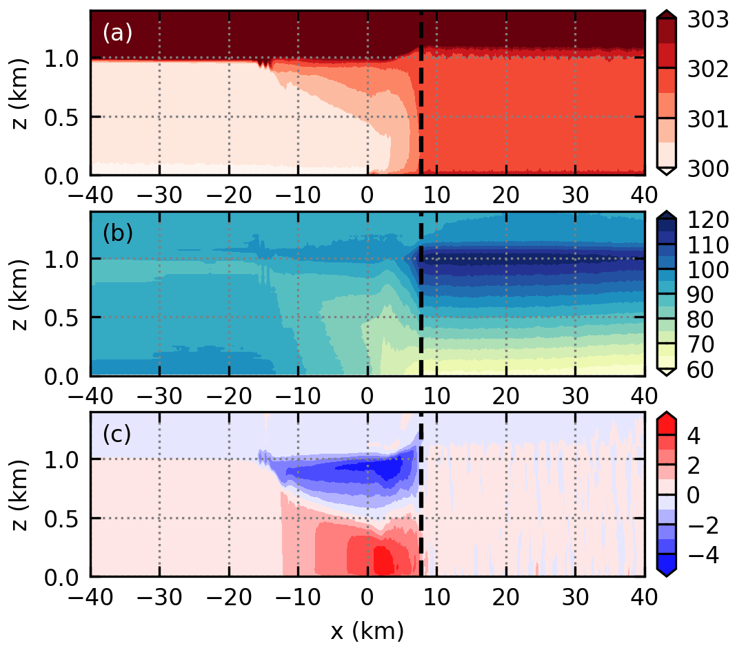
Figure 2Along-coast averaged (a) potential temperature (K), (b) full pressure perturbation (Pa), and (c) cross-coast wind (m s−1) at t=2 h in simulation SHF02. The dashed lines indicate the position of the SBF.
3.2 Formation of large updrafts near the SBF
Figure 3 shows a horizontal cross section of the cross-coast wind and the vertical velocity at z=0.5zi and at t=2 h 48 min in simulation SHF02. Figure 3a shows that streaky structures of positive cross-coast wind are produced behind the SBF. Previous studies have proposed several theories explaining the formation of streaky structures, e.g., the inflection-point instability and the convective instability (Etling and Brown, 1993; Gryschka and Raasch, 2005). The inflection-point instability relies on a sufficiently strong inflection point in the along-coast wind profile. However, no such inflection point exists in our simulations (not shown). The convective instability is usually measured with a parameter , where L is the Obukhov length (Khanna and Brasseur, 1998; Salesky et al., 2017). In the region from x=10 to 12 km and from to 3 km, calculation shows that the mean value of is 70. Based on previous studies, this value should correspond to cells instead of the streaky structures shown in Fig. 3a. Previous studies suggest that the threshold values of hold for situations where the shear is limited near the surface, while in our simulations, the shear occurs over a deep layer (Fig. 2c). It is interesting to mention that some studies suggest that wind shear alone is sufficient for the generation of streaky structures (e.g., Lee et al., 1990).
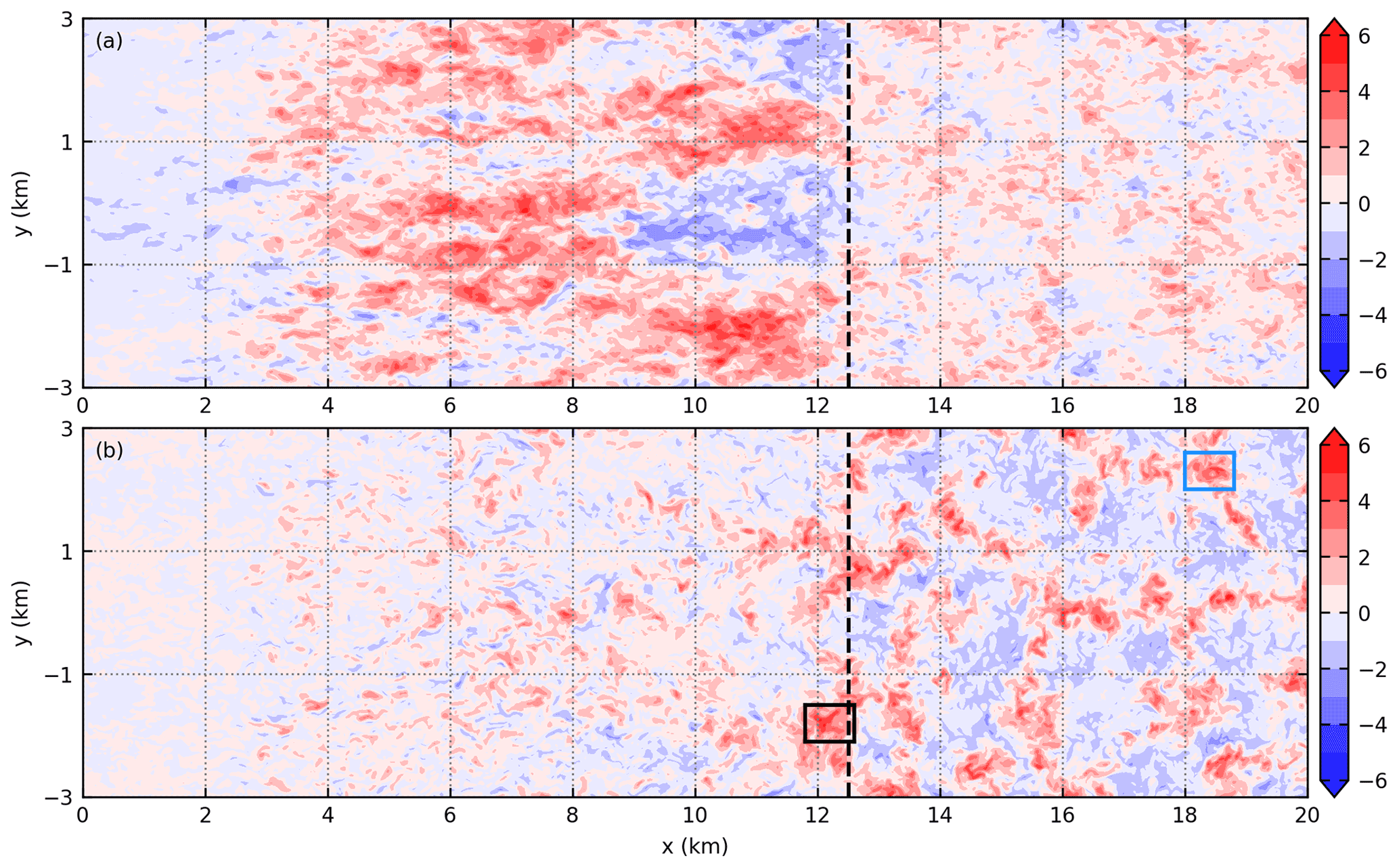
Figure 3A horizontal cross section of (a) cross-coast wind (m s−1) and (b) vertical velocity (m s−1) at z=0.5zi and at t=2 h 48 min in simulation SHF02. The dashed lines indicate the position of the SBF. The rectangles enclose the updrafts whose formation processes are investigated with parcel trajectories.
Figure 3b indicates that the updrafts near the SBF are larger than those ahead of the SBF. A comparison of Fig. 3a and b reveals that the larger updrafts near the SBF are closely related to the postfrontal streaky structures. Note that Fig. 3 is a snapshot representative of all times when large updrafts are visible (Fu, 2022). Figure 3b also shows that the updrafts far behind the SBF are generally much weaker than those near or ahead of the SBF. They are less likely to trigger convective cells and are hence not analyzed in detail.
Figure 4a shows the vertical velocity and the cross-coast wind of the composite frontal updraft at z=0.5zi. It clearly shows that the frontal updraft forms at the leading edge of the streaky structure, confirming the snapshot impression from Fig. 3. As a comparison, Fig. 4b shows that no similar structure exists near the prefrontal updraft.
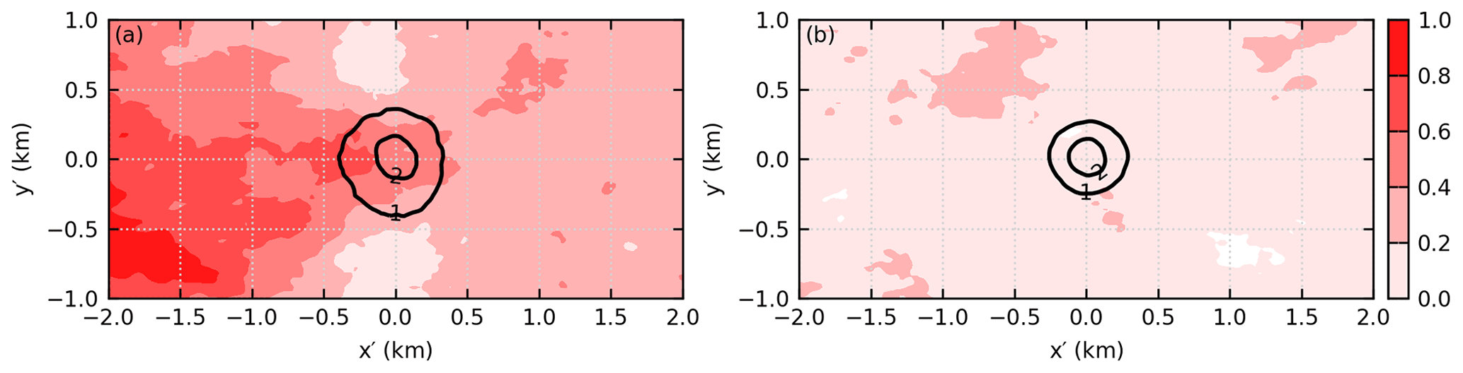
Figure 4(a) Horizontal cross section of vertical velocity (m s−1; black contour) and cross-coast wind (m s−1; filled contour) of the composite frontal updraft at z=0.5zi in simulation SHF02. (b) The same as (a) except for the composite prefrontal updraft.
Parcel trajectories are used to further analyze how the updrafts are produced. A parcel is said to cross the height z at time t if it is below the height z at time t−1 min, is above z at time t, and ascends by more than 0.12 km from time t−1 min to t (corresponding to a vertical velocity of 2 m s−1). The gray lines in Fig. 5a and b show the parcel trajectories that cross the height z=0.5zi at t=2 h 48 min through the region enclosed by the black rectangle and blue rectangle in Fig. 3b, respectively. The parcels are tracked from t=2 h 40 min to 2 h 50 min. In order to know where the parcels come from, e.g., from behind the SBF or from ahead of the SBF, they are divided into four groups by the 25th, 50th, and 75th percentiles of their x positions at t=2 h 40 min. The demarcations separating the four groups are shown with the black arrows. The colored lines in Fig. 5 show the mean parcel trajectories of each group.
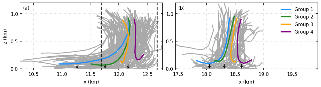
Figure 5(a) Gray lines are individual parcel trajectories that cross the region enclosed by the black rectangle in Fig. 3b. The parcels are tracked from t=2 h 40 min to 2 h 50 min in simulation SHF02. Every 50th parcel trajectory is shown. The four colored lines show the mean parcel trajectories of the four groups, respectively. The three arrows show the x positions that separate the trajectories into four groups. The left and right dashed lines indicate the position of the SBF at t=2 h 40 min and 2 h 50 min, respectively. (b) The same as (a) except for parcel trajectories that cross the region enclosed by the blue rectangle in Fig. 3b.
Ahead of the SBF (Fig. 5b), the parcels mostly ascend vertically, except near the surface, where the horizontal convergence of parcels is apparent and well understood (Stull, 1988). Near the SBF (Fig. 5a), there also exist parcels that ascend vertically, e.g., the parcels in the third and fourth groups. In addition to this, many parcels ascend along slanted trajectories, e.g., the parcels in the first and second groups. These parcels gain buoyancy from behind the SBF. They are then transported toward the SBF by the sea breeze and merge with the parcels that originate near the SBF. Note that the parcels rising from behind the SBF are part of the streaky structure. This suggests that the larger updraft near the SBF forms as a result of the merger between the streaky structure and the updraft that originates near the SBF.
The updrafts near the SBF and those ahead of the SBF are separately composited and shown in Fig. 6. It shows that the composite frontal updraft is larger than the composite prefrontal updraft, both in the x–z plane (cf. Fig. 6a and c) and in the y–z plane (cf. Fig. 6b and d), consistent with the finding of Fu et al. (2021). It is also found that the maximum vertical velocity of the composite frontal updraft is similar to that of the composite prefrontal updraft, with a difference of less than 10 %, again consistent with the finding of Fu et al. (2021). We note that the resolution used by Fu et al. (2021) is 100 m in the horizontal and 40 m in the vertical, while the resolution used in this study is 20 m both in the horizontal and in the vertical. This means that our conclusion is independent of model resolution.
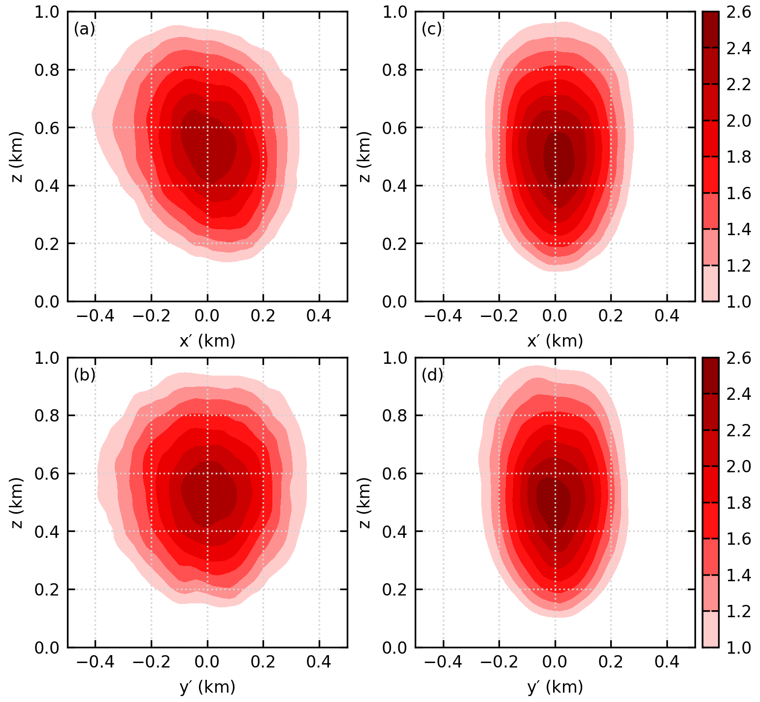
Figure 6(a) x–z cross section and (b) y–z cross section of the vertical velocity (m s−1) of the composite frontal updraft in simulation SHF02. Panels (c) and (d) are the same as panels (a) and (b) except for the composite prefrontal updraft.
3.3 Lagrangian budget analysis of vertical momentum
The budget of vertical momentum along the parcel trajectories is analyzed to investigate whether the dynamical forcing of the updrafts near the SBF is different from that ahead of the SBF. The Lagrangian vertical momentum equation is
where w is vertical velocity, the reference density, and the dynamic pressure perturbation. The effective buoyancy beff is
where b is buoyancy, and is the buoyancy pressure perturbation. The pressure perturbations satisfy
where v is the velocity vector. Following Markowski and Richardson (2010, p. 29), is calculated by solving Eq. (5), and is then obtained by subtracting from the full pressure perturbation.
In the Lagrangian budget analysis, we include only those parcels that continuously ascend to the top of the boundary layer. For each parcel, the first time it rises above z=0.9 km is defined as ttop. We then search backward in time to find the period during which the parcel ascends continuously and define the start of this period as tlift. The history between tlift and ttop is used for the budget analysis. In addition, a parcel is defined as near the SBF if its x position (xp) satisfies xSBF−1 km <xp<xSBF+1 km throughout the continuously ascending period. A parcel is defined as ahead of the SBF if it satisfies km km throughout the ascending period. xSBF, e is the position of the SBF at 30 min after the release of the parcels.
Figure 7 shows the profiles of effective buoyancy and dynamic pressure gradient force for parcels released at t=2 h and tracked for 10 min in simulation SHF02. The effective buoyancy is positive from the surface up to z=0.9 km and then becomes negative, and the dynamic pressure gradient force is positive from the surface up to z=0.6 km and then becomes negative. The profiles of both the effective buoyancy and the dynamic pressure gradient force are similar to those of Torri et al. (2015). More importantly, the dynamics experienced by the parcels near the SBF is almost the same as that experienced by the parcels ahead of the SBF. We note that the results are similar for parcels that are released at t=2 h and tracked for 15 min (not shown), and the results are also similar for parcels that are released at t=2 h 30 min, 3 h, and 3 h 30 min, tracked for either 10 or 15 min (not shown). The similar dynamics explains the fact that the strengths of the updrafts near the SBF are similar to those ahead of the SBF. Figure 7 also shows that there is no extra dynamic pressure gradient force near the SBF. This is also different from the density-current analogy.
3.4 Persistence of the updrafts
The persistence of an updraft also affects its potential in DCI. Figure 8a shows the temporal evolution of the vertical velocity at z=0.5zi averaged from xSBF−1 km to xSBF+1 km, and Fig. 8b shows that averaged from x=30 to 32 km, a region that is ahead of the SBF throughout the simulation. It is seen that the updrafts near the SBF are generally shorter-lived than those ahead of the SBF, suggesting that the persistence of updrafts cannot explain the fact that the SBF is the more favorable region for DCI than the prefrontal region. Nevertheless, it is worth pointing out that the lifetime of the updrafts near the SBF is long enough for parcels near the surface to be lifted to the top of the boundary layer, as can be seen from Fig. 5.
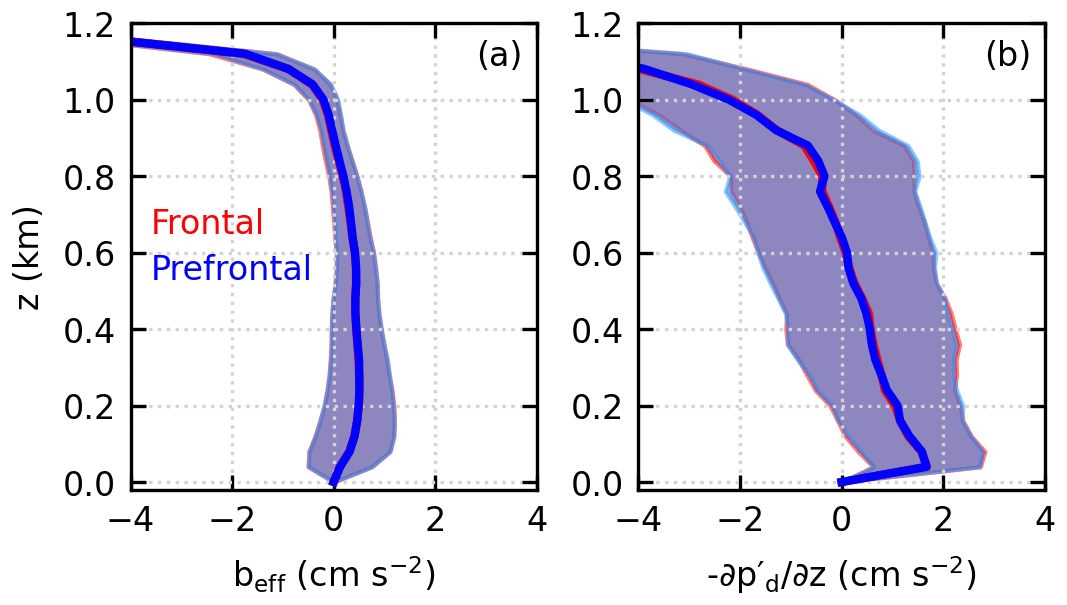
Figure 7Profiles of (a) effective buoyancy and (b) dynamic pressure gradient force along the parcel trajectories. The parcels are released at t=2 h and tracked for 10 min in simulation SHF02. The solid lines show the averages, and the shadings show the standard deviations. Note that the profiles near the SBF are almost the same as those ahead of the SBF.
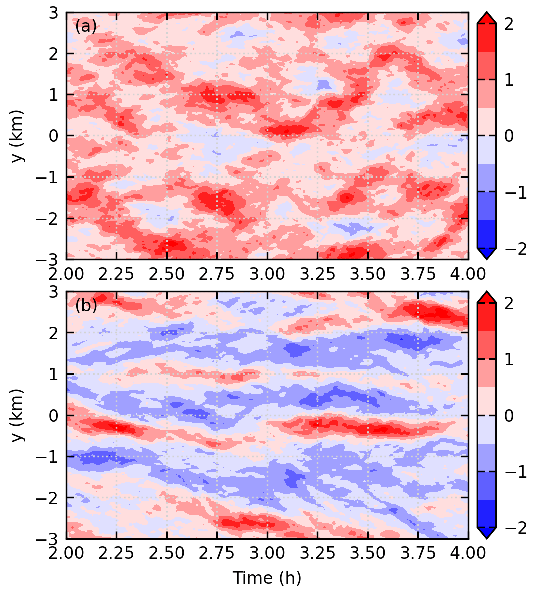
Figure 8Temporal evolution of vertical velocity (m s−1) at z=0.5zi averaged (a) from xSBF−1 km to xSBF+1 km and (b) from x=30 to 32 km in simulation SHF02.
3.5 Sensitivity to SHF and environmental wind
We now discuss the sensitivity of the results to SHF and environmental wind. Table 1 lists the xSBF, zi, and w* at the end of the simulations. It also lists the horizontal convergence at the SBF averaged from t=2 to 4 h. The horizontal convergence is calculated as described in Sect. 2.2. In the simulations without environmental wind (i.e., simulations SHF01, SHF02, and SHF03), increasing SHF from 0.1 to 0.3 K m s−1 increases the propagation speed of the SBF (Antonelli and Rotunno, 2007), so the SBF moves farther inland by the end of the simulations; increasing SHF also increases the boundary-layer height, the convective velocity scale, and the mean horizontal convergence at the SBF.
Table 1The position of the SBF (xSBF), boundary-layer height (zi), and convective velocity scale (w*) at the end of the simulations and the mean horizontal convergence at the SBF averaged from t=2 to 4 h.

Compared to simulation SHF02, the SBF propagates at a slower speed in simulation SHF02_Un2 but propagates at a faster speed in simulation SHF02_Up2, consistent with previous studies (Miller et al., 2003). Thus, the SBF moves less inland in simulation SHF02_Un2 but farther inland in simulation SHF02_Up2 than that in simulation SHF02. Table 1 also indicates that neither the boundary-layer height nor the convective velocity scale is sensitive to the environmental wind. However, the mean horizontal convergence at the SBF is sensitive to the environmental wind: a negative environmental wind increases the convergence, while a positive environmental wind decreases the convergence.
In all the simulations considered in this study, the frontal updrafts are produced at the leading edge of the postfrontal streaky structures (not shown), and the dynamics experienced by the parcels constituting the updrafts near the SBF is nearly the same as that ahead of the SBF (not shown), as seen in simulation SHF02.
In a classical convective boundary layer, such as that ahead of the SBF, it is well known that the size of the updraft scales with zi and the strength of the updraft scales with w* (Stull, 1988). Since the dynamics of the frontal updrafts is similar to that of the prefrontal updrafts, it is expected that this scaling is also applicable for frontal updrafts. In order to test this speculation, we re-composited the updrafts using a slightly different procedure. At each output time, the size is normalized by zi and the vertical velocity is normalized by w* before the ensemble averaging. The other steps are the same as those described in Sect. 2.2.
We first consider the three simulations without environmental wind, which are shown with Fig. 9. Ahead of the SBF (Fig. 9c and d), the composite normalized updrafts are similar for all three simulations, as is well known. More importantly, the composite normalized updrafts near the SBF are also similar for all three simulations (Fig. 9a and b). This means that the aforementioned scaling also works for the frontal updrafts when the environmental wind is zero. Note that, although the composite normalized updrafts are similar in both size and strength in all three simulations, the composite dimensional updrafts actually become larger and stronger as SHF increases, as can be deduced from the increasing zi and w* (Table 1). In each simulation, Fig. 9 also shows that the frontal updraft is larger than the prefrontal updraft and that their strengths are similar.
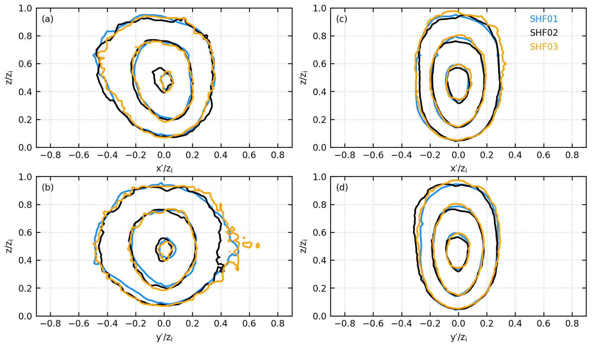
Figure 9(a) x–z cross section and (b) y–z cross section of the normalized vertical velocity of the composite normalized frontal updraft in simulations SHF01, SHF02, and SHF03. The contour levels are 0.4, 0.8, and 1.2. Panels (c) and (d) are the same as panels (a) and (b), except for the composite normalized prefrontal updraft.
We next consider the three simulations with varying environmental wind, which are shown with Fig. 10. Ahead of the SBF, the composite normalized updrafts are similar in the y–z cross section for all three simulations (Fig. 10d). In the x–z cross section (Fig. 10c), the updraft slightly tilts downwind due to the environmental wind. Near the SBF, Fig. 10a and b show that the composite normalized frontal updrafts are substantially different among the three simulations. In the x–z cross section (Fig. 10a), the frontal updrafts tilt to the left in all three simulations; however, the frontal updraft is less tilted in simulation SHF02_Up2 and is more tilted in simulation SHF02_Un2. This is because a positive environmental wind reduces the wind shear, while a negative environmental wind enhances the wind shear near the SBF.

In the y–z cross section (Fig. 10b), the composite normalized frontal updrafts are similar in the z direction but are very different in the y direction. In simulation SHF02_Un2, the negative wind enhances the convergence near the SBF (Table 1). More updrafts are therefore transported toward the SBF. Their merger produces a wider updraft in the y direction. In simulation SHF02_Up2, the positive environmental wind weakens the convergence near the SBF (Table 1). Fewer updrafts are transported to the SBF, and their merger produces a narrower updraft in the y direction. Nevertheless, Fig. 10 clearly shows that the frontal updrafts are larger than and have similar strength to the prefrontal updrafts in all three simulations with environmental wind.
Based on the results of Antonelli and Rotunno (2007), the y-averaged cross-coast wind and , where N is the Brunt–Väisälä frequency. In this study, we do not vary N, and we compare the simulation results at the same time t, so we drop the nondimensional factor Nt from the aforementioned scaling, leading to
Substituting Eq. (7) into (1), we obtain .
Based on our analysis in Sect. 3.2, it is the convergence that affects the size of the frontal updrafts. The convergence near the SBF is measured by . When the environmental wind is zero, the convergence , where WSBF is the width of the SBF. Since and Fig. 9 suggests that the effect of convergence does not introduce scales other than zi and w*, we obtain that WSBF∼zi. This means that the width of the SBF is approximately 1 km in this study (Table 1). The observational study by Chiba (1993) found that the width of the SBF was between 0.13 and 1.12 km. When the environmental wind is not zero, the convergence , where U is the environmental wind. Since U is an independent parameter, it does not scale with w*. As a result, does not scale with w* either. In this situation, the simple scaling breaks down, as seen in Fig. 10.
The sea-breeze circulation (SBC) is frequently found to play an important role in deep-convection initiation (DCI). Previous studies have found that the sea-breeze front (SBF) is a more favorable region for DCI than the prefrontal region. A recent study by Fu et al. (2021) showed that the updrafts near the SBF are larger and moister than the updrafts ahead of the SBF, so that DCI occurs preferentially near the SBF. However, they did not explain why the updrafts near the SBF are larger, and they did not explain why the updrafts near and ahead of the SBF have similar strengths.
This study performs a series of large-eddy simulations to investigate the size and strength of the updrafts near the SBF and to compare the characteristics of updrafts near the SBF to those ahead of the SBF. Similar to Fu et al. (2021), it is found that the updrafts near the SBF are larger than those ahead of the SBF. It is further shown here that the larger updrafts near the SBF are produced through the merger between the postfrontal streaky structures and the updrafts that originate near the SBF. It is also shown that the updrafts near the SBF have similar strengths to those ahead of the SBF, consistent with the finding of Fu et al. (2021). This is further investigated here through a Lagrangian budget analysis of the vertical-momentum equation. The results reveal that the dynamics experienced by the parcels constituting the updrafts near the SBF is almost the same as that ahead of the SBF, which explains why the strength of the updrafts near the SBF is similar to that ahead of the SBF.
In the typical convective boundary layer ahead of the SBF, the size and the strength of the updrafts scale with the boundary-layer height and the convective velocity scale, respectively, as is well known. Our results further reveal that this scaling also works for the updrafts near the SBF when the environmental wind is not included; however, this scaling breaks down when an environmental wind is included.
Surface heterogeneities can produce inland breezes (e.g., van Heerwaarden et al., 2014), which are also capable of triggering deep convection (Patton et al., 2005; Kang and Bryan, 2011; Rieck et al., 2014; Huang et al., 2019). Both sea breezes and inland breezes are produced by differential heating, so they are dynamically very similar. It is expected that the results in this study also apply to inland breezes.
The CM1 model is publicly available at https://www2.mmm.ucar.edu/people/bryan/cm1/ (Bryan, 2022). Additional information can be accessed at https://doi.org/10.17605/OSF.IO/3HYPS (Fu, 2022). Please contact Shizuo Fu for the model output data.
SF and RR designed the study. SF performed the simulations. All the authors commented on the results and co-wrote the paper.
The contact author has declared that neither they nor their co-authors have any competing interests.
Publisher’s note: Copernicus Publications remains neutral with regard to jurisdictional claims in published maps and institutional affiliations.
We thank George Bryan for providing the CM1 model and the National Supercomputer Center in Guangzhou for technical support.
This research has been supported by the National Natural Science Foundation of China (grant nos. 42105080 and 41930968). The National Center for Atmospheric Research is sponsored by the National Science Foundation.
This paper was edited by Holger Tost and reviewed by two anonymous referees.
Antonelli, M. and Rotunno, R.: Large-eddy simulation of the onset of the sea breeze, J. Atmos. Sci., 64, 4445–4457, https://doi.org/10.1175/2007JAS2261.1, 2007.
Bechtold, P., Pinty, J.-P., and Mascart, P.: A numerical investigation of the influence of large-scale winds on sea-breeze- and inland-breeze-type Circulations, J. Appl. Meteor., 30, 1268–1279, 1991.
Benjamin, T. B.: Gravity currents and related phenomena, J. Fluid Mech., 31, 209–248, 1968.
Borne, K., Chen, D., and Nunez, M.: A method for finding sea breeze days under stable synoptic conditions and its application to the Swedish west coast, Int. J. Climatol., 18, 901–914, 1998.
Bryan, G.: Cloud Model 1, NCAR [code], https://www2.mmm.ucar.edu/people/bryan/cm1/ (last access: 8 October 2021), 2022.
Bryan, G. H. and Fritsch, J. M.: A benchmark simulation for moist nonhydrostatic numerical models, Mon. Weather Rev., 130, 2917–2928, https://doi.org/10.1175/1520-0493(2002)130<2917:ABSFMN>2.0.CO;2, 2002.
Bryan, G. H. and Rotunno, R.: Gravity currents in confined channels with environmental shear, J. Atmos. Sci., 71, 1121–1142, https://doi.org/10.1175/JAS-D-13-0157.1, 2014.
Carbone, R. E., Wilson, J. W., Keenan, T. D., and Hacker, J. M.: Tropical island convection in the absence of significant topography. Part I: Life cycle of diurnally forced convection, Mon. Weather Rev., 128, 3459–3480, https://doi.org/10.1175/1520-0493(2000)128<3459:TICITA>2.0.CO;2, 2000.
Chiba, O.: The turbulent characteristics in the lowest part of the sea breeze front in the atmospheric surface layer, Bound.-Lay. Meteorol., 65, 181–195, https://doi.org/10.1007/BF00708823, 1993.
Crosman, E. T. and Horel, J. D.: Sea and lake breezes: A review of numerical studies, Bound.-Lay. Meteorol., 137, 1–29, https://doi.org/10.1007/s10546-010-9517-9, 2010.
Crosman, E. T. and Horel, J. D.: Idealized large-eddy simulations of sea and lake breezes: Sensitivity to lake diameter, heat flux and stability, Bound.-Lay. Meteorol., 144, 309–328, https://doi.org/10.1007/s10546-012-9721-x, 2012.
Cuxart, J., Jiménez, M. A., Telišman Prtenjak, M., and Grisogono, B.: Study of a sea-breeze case through momentum, temperature, and turbulence budgets, J. Appl. Meteor. Climatol., 53, 2589–2609, https://doi.org/10.1175/JAMC-D-14-0007.1, 2014.
Dauhut, T., Chaboureau, J.-P., Escobar, J., and Mascart, P.: Giga-LES of hector the convector and its two tallest updrafts up to the stratosphere, J. Atmos. Sci., 73, 5041–5060, https://doi.org/10.1175/JAS-D-16-0083.1, 2016.
Deardorff, J. W.: Stratocumulus-capped mixed layers derived from a three-dimensional model, Bound.-Lay. Meteorol., 18, 495–527, https://doi.org/10.1007/BF00119502, 1980.
Etling, D. and Brown, R. A.: Roll vortices in the planetary boundary layer: A review, Bound.-Lay. Meteorol, 65, 215–248, https://doi.org/10.1007/BF00705527, 1993.
Fu, S.: Updrafts near SBF, OSF, https://doi.org/10.17605/OSF.IO/3HYPS, 2022.
Fu, S., Deng, X., Li, Z., and Xue, H.: Radiative effect of black carbon aerosol on a squall line case in North China, Atmos. Res., 197, 407–414, https://doi.org/10.1016/j.atmosres.2017.07.026, 2017.
Fu, S., Rotunno, R., Chen, J., Deng, X., and Xue, H.: A large-eddy simulation study of deep-convection initiation through the collision of two sea-breeze fronts, Atmos. Chem. Phys., 21, 9289–9308, https://doi.org/10.5194/acp-21-9289-2021, 2021.
Grant, L. D. and van den Heever, S. C.: Cold pool dissipation, J. Geophys. Res.-Atmos., 121, 1138–1155, https://doi.org/10.1002/2015JD023813, 2016.
Gryschka, M. and Raasch, S.: Roll convection during a cold air outbreak: A large eddy simulation with stationary model domain, Geophys. Res. Lett., 32, L14805, https://doi.org/10.1029/2005GL022872, 2005.
Huang, Y., Meng, Z., Li, W., Bai, L., and Meng, X.: General features of radar-observed boundary layer convergence lines and their associated convection over a sharp vegetation-contrast area, Geophys. Res. Lett., 46, 2865–2873, https://doi.org/10.1029/2018GL081714, 2019.
Kang, S.-L. and Bryan, G. H.: A large-eddy simulation study of moist convection initiation over heterogeneous surface fluxes, Mon. Weather Rev., 139, 2901–2917, https://doi.org/10.1175/MWR-D-10-05037.1, 2011.
Khanna, S. and Brasseur, J. G.: Three-dimensional buoyancy- and shear-induced local structure of the atmospheric boundary layer, J. Atmos. Sci., 55, 710–743, https://doi.org/10.1175/1520-0469(1998)055<0710:TDBASI>2.0.CO;2, 1998.
Klemp, J. B. and Wilhelmson, R. B.: The simulation of three-dimensional convective storm dynamics, J. Atmos. Sci., 35, 1070–1096, 1978.
Koch, S. E. and Clark, W. L.: A nonclassical cold front observed during COPS-91: Frontal structure and the process of severe storm initiation, J. Atmos. Sci., 56, 2862–2890, https://doi.org/10.1175/1520-0469(1999)056<2862:ANCFOD>2.0.CO;2, 1999.
Koch, S. E. and Ray, C. A.: Mesoanalysis of summertime convergence zones in central and eastern North Carolina, Weather Forecast., 12, 56–77, https://doi.org/10.1175/1520-0434(1997)012<0056:MOSCZI>2.0.CO;2, 1997.
Kraus, H., Hacker, J. M., and Hartmann, J.: An observational aircraft-based study of sea-breeze frontogenesis, Bound.-Lay. Meteorol., 53, 223–265, 1990.
Lee, M. J., Kim, J., and Moin, P.: Structure of turbulence at high shear rate, J. Fluid Mech., 216, 561–583, 1990.
Markowski, P. M. and Richardson, Y.: Mesoscale meteorology in midlatitudes, John Wiley & Sons, Ltd, 407 pp., ISBN 978-0-470-74213-6, 2010.
Miller, S. T. K., Keim, B. D., Talbot, R. W., and Mao, H.: Sea breeze: structure, forecasting, and impacts, Rev. Geophys., 41, 3, https://doi.org/10.1029/2003RG000124, 2003.
Papanastasiou, D. K. and Melas, D.: Climatology and impact on air quality of sea breeze in an urban coastal environment, Int. J. Climatol., 29, 305–315, https://doi.org/10.1002/joc.1707, 2009.
Park, J. M., Heever, S. C., Igel, A. L., Grant, L. D., Johnson, J. S., Saleeby, S. M., Miller, S. D., and Reid, J. S.: Environmental controls on tropical sea breeze convection and resulting aerosol redistribution, J. Geophys. Res.-Atmos., 125, e2019JD031699, https://doi.org/10.1029/2019JD031699, 2020.
Patton, E. G., Sullivan, P. P., and Moeng, C.-H.: The influence of idealized heterogeneity on wet and dry planetary boundary layers coupled to the land surface, J. Atmos. Sci., 62, 2078–2097, https://doi.org/10.1175/JAS3465.1, 2005.
Perez, G. M. P. and Silva Dias, M. A. F.: Long-term study of the occurrence and time of passage of sea breeze in São Paulo, 1960–2009, Int. J. Climatol., 37, 1210–1220, https://doi.org/10.1002/joc.5077, 2017.
Reible, D. D., Simpson, J. E., and Linden, P. F.: The sea breeze and gravity-current frontogenesis, Q. J. Roy. Meteor. Soc., 119, 1–16, 1993.
Rieck, M., Hohenegger, C., and van Heerwaarden, C. C.: The influence of land surface heterogeneities on cloud size development, Mon. Weather Rev., 142, 3830–3846, https://doi.org/10.1175/MWR-D-13-00354.1, 2014.
Robinson, F. J., Patterson, M. D., and Sherwood, S. C.: A numerical modeling study of the propagation of idealized sea-breeze density currents, J. Atmos. Sci., 70, 653–668, https://doi.org/10.1175/JAS-D-12-0113.1, 2013.
Rotunno, R., Klemp, J., and Weisman, M. L.: A theory for strong, long-lived squall lines, J. Atmos. Sci., 45, 463–485, 1988.
Salesky, S. T., Chamecki, M., and Bou-Zeid, E.: On the nature of the transition between roll and cellular organization in the convective boundary layer, Bound.-Lay. Meteorol., 163, 41–68, https://doi.org/10.1007/s10546-016-0220-3, 2017.
Schmidt, H. and Schumann, U.: Coherent structure of the convective boundary layer derived from large-eddy simulations, J. Fluid Mech., 200, 511–562, https://doi.org/10.1017/S0022112089000753, 1989.
Shen, L., Zhao, C., and Yang, X.: Climate-driven characteristics of sea-land breezes over the globe, Geophys. Res. Lett., 48, e2020GL092308, https://doi.org/10.1029/2020GL092308, 2021.
Simpson, J. E.: A comparison between laboratory and atmospheric density currents, Q. J. Roy. Meteor. Soc., 95, 758–765, https://doi.org/10.1002/qj.49709540609, 1969.
Simpson, J. E.: Gravity currents in the laboratory, atmosphere, and ocean, Annu. Rev. Fluid Mech., 14, 213–234, 1982.
Stephan, K., Kraus, H., Ewenz, C. M., and Hacker, J. M.: Sea-breeze front variations in space and time, Meteorol. Atmos. Phys., 70, 81–95, https://doi.org/10.1007/s007030050026, 1999.
Stull, R. B.: An introduction to boundary layer meteorology, 1st edn., Kluwer Academic Publishers, 670 pp., ISBN 978-90-277-2769-5, 1988.
Sullivan, P. P. and Patton, E. G.: The effect of mesh resolution on convective boundary layer statistics and structures generated by large-eddy simulation, J. Atmos. Sci., 68, 2395–2415, https://doi.org/10.1175/JAS-D-10-05010.1, 2011.
Torri, G., Kuang, Z., and Tian, Y.: Mechanisms for convection triggering by cold pools, Geophys. Res. Lett., 42, 1943–1950, https://doi.org/10.1002/2015GL063227, 2015.
van Heerwaarden, C. C., Mellado, J. P., and De Lozar, A.: Scaling Laws for the Heterogeneously Heated Free Convective Boundary Layer, J. Atmos. Sci., 71, 3975–4000, https://doi.org/10.1175/JAS-D-13-0383.1, 2014.
Wieringa: Representative roughness parameters for homogeneous terrain, Bound.-Lay. Meteorol., 63, 323–363, 1993.
Wood, R., Stromberg, I. M., and Jonas, P. R.: Aircraft observations of sea-breeze frontal structure, Q. J. Roy. Meteor. Soc., 125, 1959–1995, 1999.
Yang, F., Ovchinnikov, M., and Shaw, R. A.: Long-lifetime ice particles in mixed-phase stratiform clouds: Quasi-steady and recycled growth, J. Geophys. Res.-Atmos., 120, 11617–11635, https://doi.org/10.1002/2015JD023679, 2015.
Yang, Y., He, G.-W., and Wang, L.-P.: Effects of subgrid-scale modeling on Lagrangian statistics in large-eddy simulation, J. Turbul., 9, N8, https://doi.org/10.1080/14685240801905360, 2008.
Yu, L. and Weller, R. A.: Objectively Analyzed Air–Sea Heat Fluxes for the Global Ice-Free Oceans (1981–2005), B. Am. Meteorol. Soc., 88, 527–540, https://doi.org/10.1175/BAMS-88-4-527, 2007.