Measurement report: Spectral and statistical analysis of aerosol hygroscopic growth from multi-wavelength lidar measurements in Barcelona, Spain

This paper presents the estimation of the hygroscopic growth parameter of atmospheric aerosols retrieved with a multi-wavelength lidar, a micro-pulse lidar (MPL) and daily radiosoundings in the coastal region of Barcelona, Spain. The hygroscopic growth parameter, γ, parameterizes the magnitude of the scattering enhancement in terms of the backscatter coefficient following Hänel parameterization. After searching for time-colocated lidar and radiosounding measurements (performed twice a day, all year round at 00:00 and 12:00 UTC), a strict criterion-based procedure (limiting the variations of magnitudes such as water vapor mixing ratio (WMVR), potential temperature, wind speed and direction) is applied to select only cases of aerosol hygroscopic growth. A spectral analysis (at the wavelengths of 355, 532 and 1064 nm) is performed with the multi-wavelength lidar, and a climatological one, at the wavelength of 532 nm, with the database of both lidars. The spectral analysis shows that below 2 km the regime of local pollution and sea salt γ decreases with increasing wavelengths. Since the 355 nm wavelength is sensitive to smaller aerosols, this behavior could indicate slightly more hygroscopic aerosols present at smaller size ranges. Above 2 km (the regime of regional pollution and residual sea salt) the values of γ at 532 nm are nearly the same as those below 2 km, and its spectral behavior is flat. This analysis and others from the literature are put together in a table presenting, for the first time, a spectral analysis of the hygroscopic growth parameter of a large variety of atmospheric aerosol hygroscopicities ranging from low (pure mineral dust, γ <0.2) to high (pure sea salt, γ > 1.0) hygroscopicity. The climatological analysis shows that, at 532 nm, γ is rather constant all year round and has a large monthly standard deviation, suggesting the presence of aerosols with different hygroscopic properties all year round. The annual γ is 0.55 ± 0.23. The height of the layer where hygroscopic growth was calculated shows an annual cycle with a maximum in summer and a minimum in winter. Former works describing the presence of recirculation layers of pollutants injected at various heights above the planetary boundary layer (PBL) may explain why γ, unlike the height of the layer where hygroscopic growth was calculated, is not season-dependent. The subcategorization of the whole database into No cloud and Below-cloud cases reveals a large difference of γ in autumn between both categories (0.71 and 0.33, respectively), possibly attributed to a depletion of inorganics at the point of activation into cloud condensation nuclei (CCN) in the Below-cloud cases. Our work calls for more in situ measurements to synergetically complete such studies based on remote sensing.

1 Introduction

Atmospheric aerosols and water vapor are atmospheric components of extreme importance for the climate on Earth. Atmospheric aerosols influence the energy balance between the Earth and the atmosphere, directly through their scattering and absorbing interaction with the electromagnetic radiation (Thorsen et al., 2020), and indirectly by modifying the thermodynamic profiles (semi-direct effect, Hansen et al., 1997; Koren et al., 2004) or changing cloud properties, including their lifetime and albedo (indirect effects, Seinfeld et al., 2016). Generally, the aerosol effects on the Earth–atmosphere energy budget depend on the aerosol optical, microphysical and radiative properties, their lifetime in the atmosphere, synoptic conditions and other factors like water vapor. The latter, being the most important primary component for the formation of clouds to occur, also has an effect on the aerosol size distribution and thus on their optical and microphysical properties. Indeed some aerosol types may increase in size due to water uptake under high relative humidity (RH) conditions. This process is called hygroscopic growth (Hänel, 1976). It is determined mainly by the aerosol chemical composition and in particular by the mixing of inorganic and organic components (Sjogren et al., 2007). Remarkably, the hygroscopic growth plays an important role in the aerosol–cloud interaction (Kanakidou et al., 2005).

The capability of aerosols to grow hygroscopically is linked to their chemical composition (Orr et al., 1958). Atmospheric aerosols can be classified as hydrophobic (e.g., dust) or hydrophilic with a monotonic (smoothly varying, e.g., volcanic) or deliquescent (step change, e.g., marine) growth type (Carrico et al., 2003). For deliquescent cases, a hygroscopic dry material exposed to increasing RH will only start to grow in size when the deliquescence RH is reached. The deliquescence RH corresponds to the equilibrium RH over an aqueous saturated solution with respect to its solute. Further increases in RH result in continued droplet growth. After deliquescence and upon exposure to decreasing RH, the aqueous droplet can form a metastable droplet, supersaturated with respect to solute concentration, until a lower crystallization (also called efflorescence by other authors, e.g., Sjogren et al., 2007) RH is reached (Tang et al., 1995; Cziczo et al., 1997; Hansson et al., 1998). As a result, the humidogram (the representation of a variable as a function of RH) of the particle size or of its optical properties usually presents a strong hysteresis with a lower branch (humidification) and upper branch (dehydration), which intercepts at or near the deliquescent and crystallization RH. As an example, measurements of pure salts of NaCl performed in the field during ACE-Asia yielded a deliquescent and crystallization RH of 75 % and 41 % (Carrico et al., 2003), respectively.

The response of aerosols to changes in RH can be measured by a variety of instruments. In the last decade, active remote sensing systems, like lidars, have revealed adequate techniques for the identification and analysis of the aerosol hygroscopic growth compared to more traditional instruments like humidified tandem nephelometers (Covert et al., 1972) and spectrometers (Gordon et al., 2015). The advantages of active remote sensing systems are multiple: they provide high vertical and temporal resolutions, they preserve the ambient conditions (no humidification or dehydration is applied on the sample), they can measure under RHs close to saturation. In the literature the aerosol hygroscopic enhancement has been measured more often on the backscatter coefficient derived from lidar (Feingold and Morley, 2003; Fernández et al., 2015; Granados-Muñoz et al., 2015; Haarig et al., 2017; Lv et al., 2017; Navas-Guzmán et al., 2019; Chen et al., 2019; Pérez-Ramírez et al., 2021) and ceilometer (Bedoya-Velásquez et al., 2019) measurements than on the extinction coefficient derived from lidar measurements (Veselovskii et al., 2009; Dawson et al., 2020). Some intents to work on the attenuated backscatter coefficient derived from ceilometers were performed by Haeffelin et al. (2016) to help track the activation of aerosols into fog or low-cloud droplets. Others investigated the lidar ratio changes due to RH and their effect on the classical elastic-backscatter lidar inversion technique (Zhao et al., 2017).

The present work takes advantage of unique observational capabilities at the site of Barcelona, NE Spain: a multi-wavelength lidar system that has been measuring at three elastic wavelengths since 2011, a single wavelength micro-pulse lidar (MPL) working continuously 24/7 since 2015, as well as two radiosoundings launched everyday almost colocated to the lidars (the database started in 2009). The paper deals with (1) the spectral analysis of the hygroscopic growth factor measured at three wavelengths, and (2) the climatological analysis of the hygroscopic growth measured at 532 nm in Barcelona. The spectral analysis is motivated by conclusions from Dawson et al. (2020), who say that multispectral lidars are fundamental to “provide additional insight into the [hygroscopic enhancement factor] retrievals since the 355 nm wavelength is sensitive to smaller aerosols than the 532 nm wavelength”. Aerosol mixing presents a clear limitation of that technique and it is discussed next. The climatological analysis is a partial answer to the call of several authors, like Bedoya-Velásquez et al. (2018), for further investigation extending the study periods to obtain results statistically that are more robust. The structure of the paper is as follows: Sect. 2 describes the instrumentations and the methodology and Sect. 3 presents the results of the spectral and climatological analysis. Conclusions are given in Sect. 4.

2 Instrumentation and methodology

2.1 Lidars and radiosoundings in Barcelona

All measurements presented in this paper were performed at or close to the lidar site in Barcelona at the Remote Sensing Laboratory of the Department of Signal Theory and Communications at the Universitat Politècnica de Catalunya (41.393^∘ N, 2.120^∘ E; 115 m a.s.l.). Two lidar systems were used: the multi-wavelength ($\mathrm{3}\mathit{\beta }+\mathrm{2}\mathit{\alpha }+\mathrm{2}\mathit{\delta }+$ WV) ACTRIS/EARLINET lidar and the MPL (1β+1δ). The first system is run according to a regular weekly schedule and monitor special aerosol events of interest. Aerosol optical properties from this system can be found in the ACTRIS database at https://actris.nilu.no/ (last access: 23 March 2022). The system employs a Nd:YAG laser emitting pulses of 355, 532 and 1064 nm at a repetition frequency of 20 Hz. The measurements of the ACTRIS/EARLINET system are averaged over 30 or 60 min. The retrieved backscatter coefficients at the three emitted wavelengths for the period 2010–2018 are used in this work. General details about the system can be found in Kumar et al. (2011). The MPL system runs continuously 24/7. It uses a pulsed solid-state laser emitting low-energy pulses (∼ 5–6 µJ) at a high pulse rate (2500 Hz). All MPL measurements are averaged over 60 min. A dead-time correction was applied following the manufacturer's instructions and laboratory calibrations of the detector (Campbell et al., 2002). Dark-count and after-pulse measurements were performed bi-monthly (Campbell et al., 2002; Welton and Campbell, 2002). The overlap correction was performed with an overlap estimation performed regularly by cross-comparing the MPL to the ACTRIS/EARLINET system and according to Sicard et al. (2020). The MPL data used in this work are the backscatter coefficient profiles at 532 nm retrieved during the period 2015–2018. All the MPL retrievals presented in this work were performed with in-house algorithms.

Radiosounding measurements are launched twice a day (at 00:00 and 12:00 UTC) by the Meteorological Service of Catalonia, Meteocat, at a distance of less than 1 km from the lidar site. Radiosoundings are launched automatically by a robotsonde manufactured by Ibatech. The radiosoundings provide measurements of pressure, temperature, RH and wind speed and direction. Data for the period 2010–2018 are used in the present work. At this point, it is important to note the inherent spatial drift of radiosoundings and the long integration time of the lidar data (as long as 60 min) which may cause a loss of temporal and spatial coincidence between both retrievals. This effect can be enhanced during daytime when the atmosphere may change quickly. This has been demonstrated by a recent paper from Muñoz-Porcar et al. (2021) in which profiles of water vapor mixing ratio (WVMR) retrieved with lidar and radiosoundings were compared. The authors also highlighted the high variability of the profile of RH in Barcelona due to the presence of the sea coast, the mild temperatures of the Mediterranean climate inducing regularly land-to-sea and sea-to-land breeze regimes and the local orography.

2.2 Methodology

This paper deals with the enhancement factor of the particle backscatter coefficient, β, as a function of RH, commonly denoted f_β(RH) in the literature. Since no other optical/microphysical property is considered here, the β suffix is omitted in the rest of the paper in order to alleviate the formulae. The wavelength dependency is indicated with a superscript λ. Finally, the backscatter coefficient at wavelength λ is denoted β^λ and the corresponding enhancement factor denoted f^λ(RH).

The methodology starts with the search of time-colocated lidar and radiosounding measurements within a difference smaller than ±120 min. The measurement time considered is that of the radiosoundings, namely 00:00 and 12:00 UTC. The time-colocated measurements are then analyzed to look for vertical intervals (h_min, h_max) in which a monotonic increase of the particle backscatter coefficient and of the RH occurs simultaneously. After fulfilling the initial conditions, these vertical intervals are classified as hygroscopic growth cases following a strict criterion-based procedure including

• water vapor mixing ratio, denoted WVMR (maximum variation of 2 g kg⁻¹),

• potential temperature, denoted θ (maximum variation of 2 K),

• wind speed (maximum variation of 2 m s⁻¹),

• wind direction (maximum variation of 15^∘).

For a convective boundary layer, WVMR, potential temperature and wind are conservative quantities. Applying these restrictions to their respective gradients guarantee that the layer is well mixed (Stull, 1976; Davidson et al., 1984); i.e., the aerosol size distribution is constant with height. In these conditions, changes in the backscatter coefficient can be assumed to be mainly due to the uptake of water vapor by particles and not to changes in the aerosol composition or concentration (Feingold and Morley, 2003). Moreover, for all cases, back trajectories at layer maximum and minimum altitudes (h_min and h_max) were also calculated with the HYbrid Single-Particle Lagrangian Integrated Trajectory (HYSPLIT) model (Stein et al., 2015) for verifying that all the aerosols inside the layer have the same origin. Such criteria have been applied by other authors (Granados-Muñoz et al., 2015; Navas-Guzmán et al., 2019; among others).

In order to discard the cases, including mineral dust which is known to be poorly hydrophilic, in case of doubts, the back trajectory analysis was completed with a mineral dust forecast from the NMMB/BSC-Dust model (https://ess.bsc.es/bsc-dust-daily-forecast, last access: 23 March 2022) and AERONET retrievals.

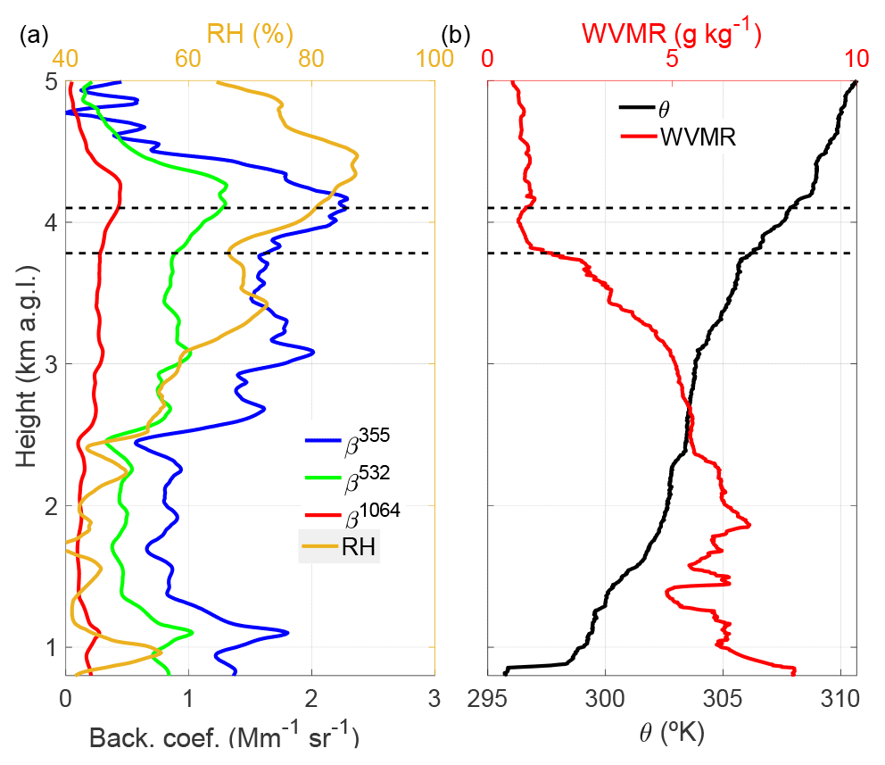
Figure 1 Vertical profiles of (a) β_λ at 3 wavelengths and RH; (b) WVMR and θ. The horizontal dash lines indicate h_min and h_max obtained by applying the criterion-based procedure. The example is from 22 July, 2013, at 13:02 UTC.

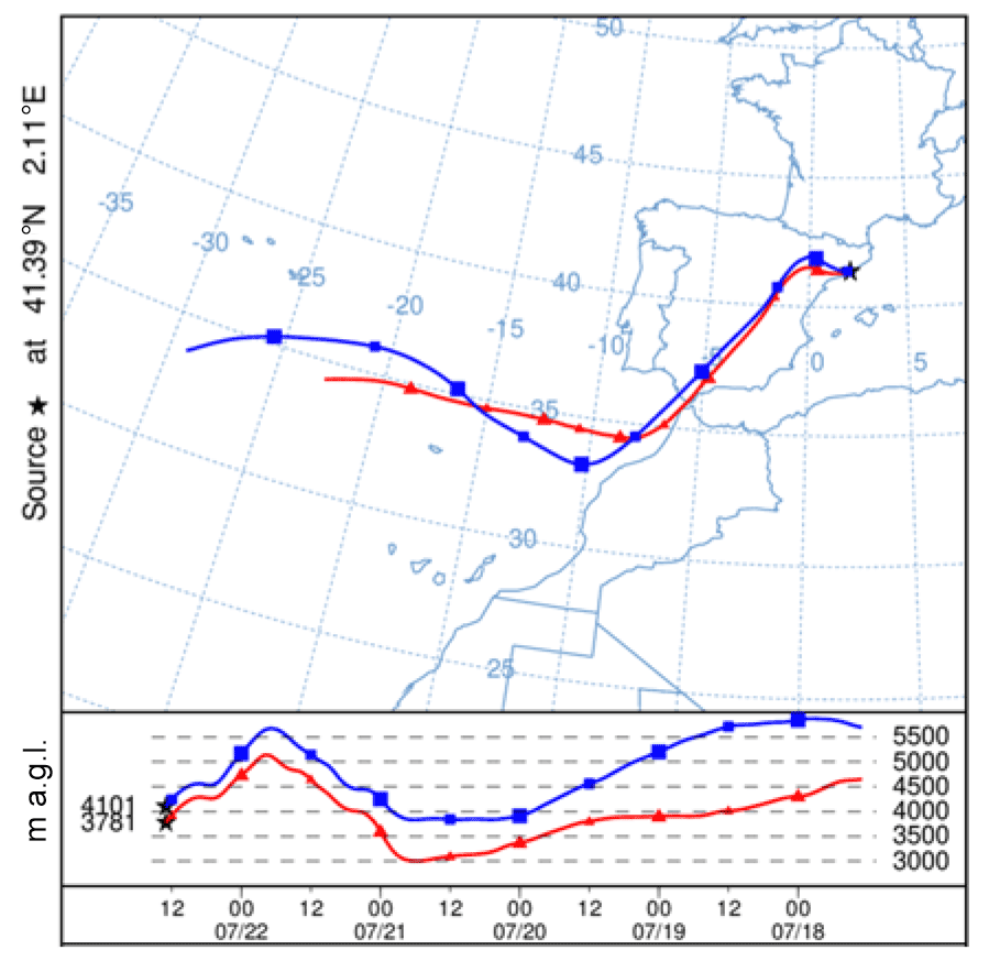
Figure 2 5 d back trajectories arriving in Barcelona on 22 July 2013, at 13:00 UTC, at h_min= 3781 m and h_max= 4101 m a.g.l.

Figure 1 is an example of one selected hygroscopic growth case. It shows the vertical profiles of β^λ at 3 wavelengths: RH, WVMR and θ. A simultaneous increase of β^λ and RH is observed inside the layer between h_min= 3781 m and h_max= 4101 m. The maximum variations of WVMR and θ inside this layer are 0.91 g kg⁻¹ and 1.63 K, respectively. The back trajectories arriving in Barcelona at h_min and h_max shown in Fig. 2 demonstrate that the air masses at the base and top of the considered layer come from the same origins – Atlantic Ocean and continental zones – ensuring that the aerosols inside the whole layer come from the same sources.

For each case, each value of β^λ in the range [h_min, h_max] has a corresponding value of RH varying in the range [RH_min, RH_max]. For each case, we define the particle backscatter coefficient enhancement factor, $f_{\min }^{\mathit{\lambda }}\left(\mathrm{RH}\right)$, defined starting from RH_min as

$$\begin{array}{}\text{(1)}& f_{\min }^{\mathit{\lambda }}\left(\mathrm{RH}\right)={\displaystyle \frac{{\mathit{\beta }}^{\mathit{\lambda }}\left(\mathrm{RH}\right)}{{\mathit{\beta }}^{\mathit{\lambda }}\left({\mathrm{RH}}_{\min }\right)}},\end{array}$$

where $f_{\min }^{\mathit{\lambda }}\left(\mathrm{RH}\right)$ quantifies the increase of β^λ when the RH increases from RH_min to RH. A fitting of $f_{\min }^{\mathit{\lambda }}\left(\mathrm{RH}\right)$ is performed with the so-called Hänel parameterization (Kasten, 1969; Sheridan et al., 2002) using the points available between RH_min and RH_max:

$$\begin{array}{}\text{(2)}& f_{\min }^{\mathit{\lambda }}\left(\mathrm{RH}\right)={\left({\displaystyle \frac{\mathrm{1}-\mathrm{RH}/\mathrm{100}}{\mathrm{1}-{\mathrm{RH}}_{\min }/\mathrm{100}}}\right)}^{-\mathit{\gamma }\left(\mathit{\lambda }\right)},\end{array}$$

where γ(λ) is the hygroscopic growth parameter and parameterizes the magnitude of the scattering enhancement. γ(λ) is totally dependent upon $f_{\min }^{\mathit{\lambda }}\left(\mathrm{RH}\right)$ but is independent of the value of RH_min chosen. While this simplified parameterization of Hänel may not work for purely deliquescent aerosols, like sea salt, it is estimated to be good enough for this study since sea salt particles, although they may often be present in the aerosol composition in Barcelona, are not the dominating species (see Sect. 3.1). The definition of the enhancement factor given in Eq. (2) limits the range of RH values for which it can be calculated, i.e., only for RH > RH_min, which prevents direct comparisons when RH_min is not the same (Veselovskii et al., 2009). In order to extend this range and have results comparable in the same range of RH values, the different functions of $f_{\min }^{\mathit{\lambda }}\left(\mathrm{RH}\right)$ are scaled to a larger range of RH values: [40 %, 90 %]. The bottom limit, 40 %, is denoted RH_ref. This reference value of 40 % has been used in several works (Skupin et al., 2016; Titos et al., 2016; Haarig et al., 2017; Bedoya-Velásquez et al., 2018; Dawson et al., 2020). RH_ref= 40 % is a recommendation of the World Meteorological Organization (World Meteorological Organization and Global Atmosphere Watch, 2003), who demonstrates with in situ measurements that the hygroscopicity growth effect on aerosols is minimized for values of RH below 40 %. The new scaled enhancement factor starting at RH_ref= 40 % is denoted $f_{\mathrm{ref}}^{\mathit{\lambda }}\left(\mathrm{RH}\right)$ and expresses the increase of β^λ when the RH increases from RH_ref to RH:

$$\begin{array}{}\text{(3)}& f_{\mathrm{ref}}^{\mathit{\lambda }}\left(\mathrm{RH}\right)={\left({\displaystyle \frac{\mathrm{1}-\mathrm{RH}/\mathrm{100}}{\mathrm{1}-R{H}_{\mathrm{ref}}/\mathrm{100}}}\right)}^{-\mathit{\gamma }\left(\mathit{\lambda }\right)}.\end{array}$$

However, when RH_min≠RH_ref, this function cannot be calculated directly. A solution is to calculate it from $f_{\min }^{\mathit{\lambda }}\left(\mathrm{RH}\right)$ as follows:

$$\begin{array}{}\text{(4)}& f_{\mathrm{ref}}^{\mathit{\lambda }}\left(\mathrm{RH}\right)=f_{\min }^{\mathit{\lambda }}\left(\mathrm{RH}\right){\left({\displaystyle \frac{\mathrm{1}-{\mathrm{RH}}_{\min }/\mathrm{100}}{\mathrm{1}-{\mathrm{RH}}_{\mathrm{ref}}/\mathrm{100}}}\right)}^{-\mathit{\gamma }\left(\mathit{\lambda }\right)}.\end{array}$$

Note that the term on the right-hand side multiplying $f_{\min }^{\mathit{\lambda }}\left(\mathrm{RH}\right)$ is nothing else than the quotient of the intercepts of both enhancement factors ($f_{\min }^{\mathit{\lambda }}$ and $f_{\mathrm{ref}}^{\mathit{\lambda }}$) at RH = 0 %. Figure 3 is an example showing the two retrieved enhancement factors $f_{\min }^{\mathit{\lambda }}$ and $f_{\mathrm{ref}}^{\mathit{\lambda }}$ and their Hänel fit. One clearly sees the difference between $f_{\min }^{\mathit{\lambda }}$ restricted to [RH_min, RH_max] (spanning 21 % in the example presented) and $f_{\mathrm{ref}}^{\mathit{\lambda }}$ spanning 50 % from 40 % to 90 %. In addition, to allow direct comparison of enhancement factors retrieved from different cases for different RH ranges, this method also has the advantage of defining a common way for the calculation of the f value. The f value, also called the f(RH) value (Titos et al., 2016), is defined as $f_{\min }^{\mathit{\lambda }}\left({\mathrm{RH}}_{\max }\right)$. It depends on both RH_min and RH_max. There is no consensus in the atmospheric community on the definition for the range of RH values which have a strong variability among studies as underlined by Titos et al. (2016). In this study, the f value is $f_{\mathrm{ref}}^{\mathit{\lambda }}\left(\mathrm{RH}=\mathrm{85}\mathit{\%}\right)$ with RH_ref= 40 %, and it applies to all cases. It expresses the increase factor of the backscatter coefficient when the RH increases from RH_ref= 40 % to 85 %.

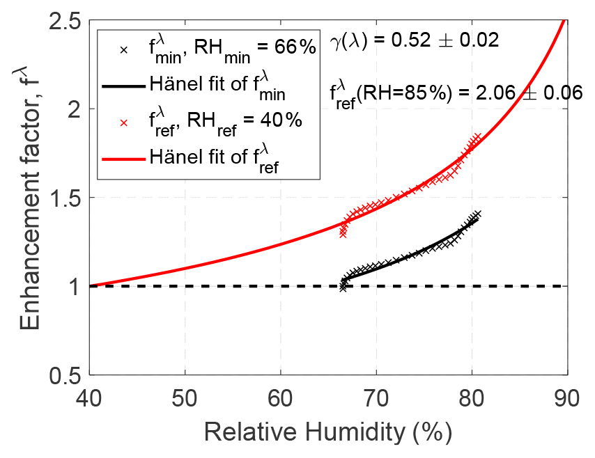
Figure 3 Example of enhancement factors $f_{\min }^{\mathit{\lambda }}$ defined starting at RH_min and $f_{\mathrm{ref}}^{\mathit{\lambda }}$ defined starting at RH_ref= 40 % of one single case (the data are those of Fig. 1: 22 July 2013, at 13:02 UTC; λ= 532 nm). The calculation of the standard errors associated with γ and $f_{\mathrm{ref}}^{\mathit{\lambda }}$ is explained in Sect. 2.3.

Finally, to avoid outliers the cases with $f_{\mathrm{ref}}^{\mathit{\lambda }}\left(\mathrm{RH}=\mathrm{85}\mathit{\%}\right)$ greater than 10 with RH_ref= 40 % (which corresponds to γ≈ 1.66) were not taken into account in the statistics.

2.3 Calculation of associated standard error

The hygroscopic growth parameter γ and its associated standard error have been estimated for each one of the analyzed cases, performing a simple linear regression after applying natural logarithms to the terms of Eq. (2). This standard error, calculated as the square root of $\frac{\mathrm{1}}{n-\mathrm{2}}$ (n being the number of points) times the sum of squares of the residuals divided by the sum of squared deviations of the predictor variable (RH) from its mean (Chatterjee and Hadi, 2006), is a measure of how precise the slope has been estimated. In this sense, it reflects the non-ideal conditions which sum up and produce a deviation of $\frac{{\mathit{\beta }}^{\mathit{\lambda }}\left(\mathrm{RH}\right)}{{\mathit{\beta }}^{\mathit{\lambda }}\left({\mathrm{RH}}_{\min }\right)}$ from its parameterization (Eq. 2) as seen in the example in Fig. 3.

For estimating the standard error of the enhancement factor at RH = 85 %, $f_{\mathrm{ref}}^{\mathit{\lambda }}(\mathrm{RH}=\mathrm{85}\mathit{\%})$, the classical error propagation formulation (Ku, 1966) has been applied to Eq. (3), taking into account estimated errors in both γ and the intercept point of the linear regression.

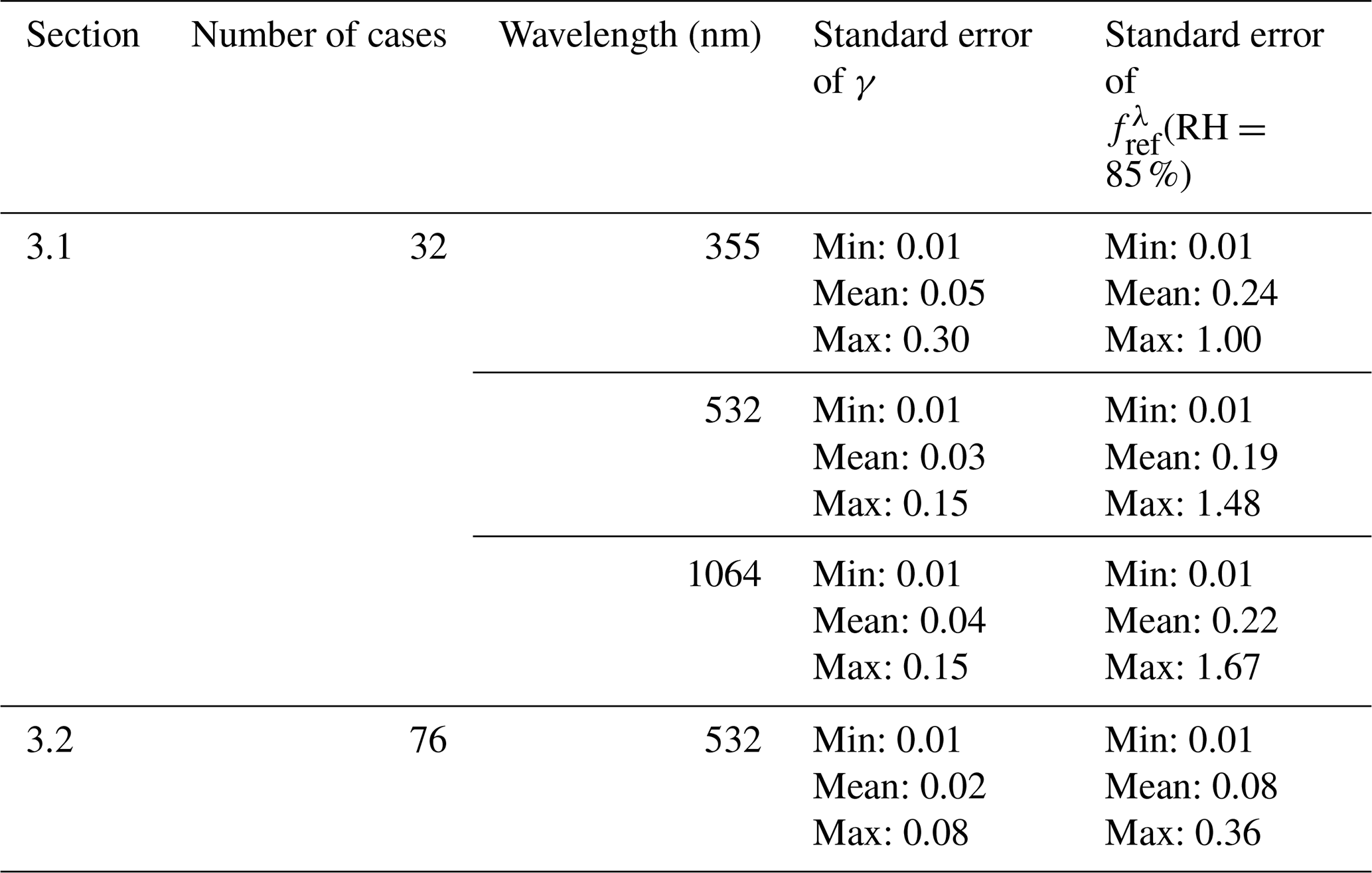
The standard errors associated with γ and $f_{\mathrm{ref}}^{\mathit{\lambda }}(\mathrm{RH}=\mathrm{85}\mathit{\%})$ calculated for all cases presented in Sect. 3 (32 in the spectral analysis and 76 in the climatological analysis) are given in Table 1. The standard error of γ is indeed small (< 0.05 on average) and is larger at 355 nm than at the other two wavelengths. The former might reflect a lower signal-to-noise ratio of the 355 nm channel of the ACTRIS/EARLINET system compared to the other two channels. The standard errors of γ for the 76 cases of the climatological analysis (0.02) are on average much smaller (by 1 order of magnitude) than the uncertainty caused by the natural variability of γ (see Sect. 3.2). The standard error of $f_{\mathrm{ref}}^{\mathit{\lambda }}(\mathrm{RH}=\mathrm{85}\mathit{\%}$) is smaller than 0.24 on average and does not seem wavelength-dependent. The standard errors of $f_{\mathrm{ref}}^{\mathit{\lambda }}(\mathrm{RH}=\mathrm{85}\mathit{\%})$ for the 76 cases of the climatological analysis (0.08) are on average much smaller (again by 1 order of magnitude) than the uncertainty caused by the natural variability of $f_{\mathrm{ref}}^{\mathit{\lambda }}(\mathrm{RH}=\mathrm{85}\mathit{\%}$). Although this analysis of associated standard errors does not account for all possible sources of error (like the error in the RH measurements which is expected to be small), the errors found are small enough for the climatological analysis presented in Sect. 3.2 to be representative of the actual natural atmospheric variations.

Table 1 Minimum, mean and maximum standard errors of γ and $f_{\mathrm{ref}}^{\mathit{\lambda }}(\mathrm{RH}=\mathrm{85}\mathit{\%})$ for the cases presented in Sect. 3.1 and 3.2.

3 Results and discussion

In this section all the standard deviations presented are the actual standard deviations associated with the variable considered and represent the natural variability of the latter.

3.1 Spectral analysis

In this section, only the ACTRIS/EARLINET lidar system (period 2010–2018), which has three elastic wavelengths, is considered. Among the backscatter profiles at the three wavelengths of 355, 532 and 1064 nm and the RH profiles from radiosoundings available between 2010–2018, 32 potential cases of hygroscopic growth which fulfilled the selection criteria mentioned in Sect. 2.2 were identified. From these 32 hygroscopic growth cases, the center of the layer considered was below 2 km a.g.l. in 8 cases (25 %) and above 2 km a.g.l. in 24 cases (75 %). This reference height of 2 km was chosen based on Sicard et al. (2006, 2011) and Pandolfi et al. (2013), who showed that the separation between the surface mixed layers and possible decoupled residual/aloft layers in the coastal area of Barcelona are more likely to occur around 2 km high. Interestingly, Pérez-Ramírez et al. (2021) also considered altitude heights below 2 km (near surface and planetary boundary layer (PBL)) and above 2 km to show the temporal evolution of f(RH) and γ. Generally speaking, in the region of Barcelona, the aerosols present below 2 km, i.e., in the PBL, are representative of a coastal, urban background site and their chemical composition is dominated by anthropogenic, crustal and marine aerosols (Querol et al., 2001). Below 2 km, the aerosol type in Barcelona is defined as local pollution and marine aerosols. According to Pey et al. (2010), the mean annual urban contribution of hydrophilic species such as ${\mathrm{SO}}_{\mathrm{4}}^{\mathrm{2}-}$, ${\mathrm{NO}}_{\mathrm{3}}^{-}$ or ${\mathrm{NH}}_{\mathrm{4}}^{+}$ in Barcelona downtown is at least 53 %, 65 % and 45 %, respectively, with respect to the regional background. For aerosol layers above 2 km, Sicard et al. (2011) refer to “recirculation polluted air masses” caused by the sea-breeze phenomenon and Pandolfi et al. (2013) to either regional or Atlantic air masses (African air masses are discarded since the cases with the presence of mineral dust are not included in this study). Above 2 km, the aerosol type in Barcelona is defined as regional pollution and marine aerosols. It is important to mention that above 2 km, the height range reaches 5 km, the approximate height where the highest top of the layer is located.

To check the provenance of the aerosol layers below and above 2 km, we plot the wind roses for the 8 cases below 2 km and the 24 cases above 2 km in Fig. 4. While the wind directions below 2 km (Fig. 4a) are diverse (NE, SSW, WSW, WNW), they are more clustered above 2 km (Fig. 4b) and almost all of them fall between SW and NNW, clearly indicating a peninsular origin.

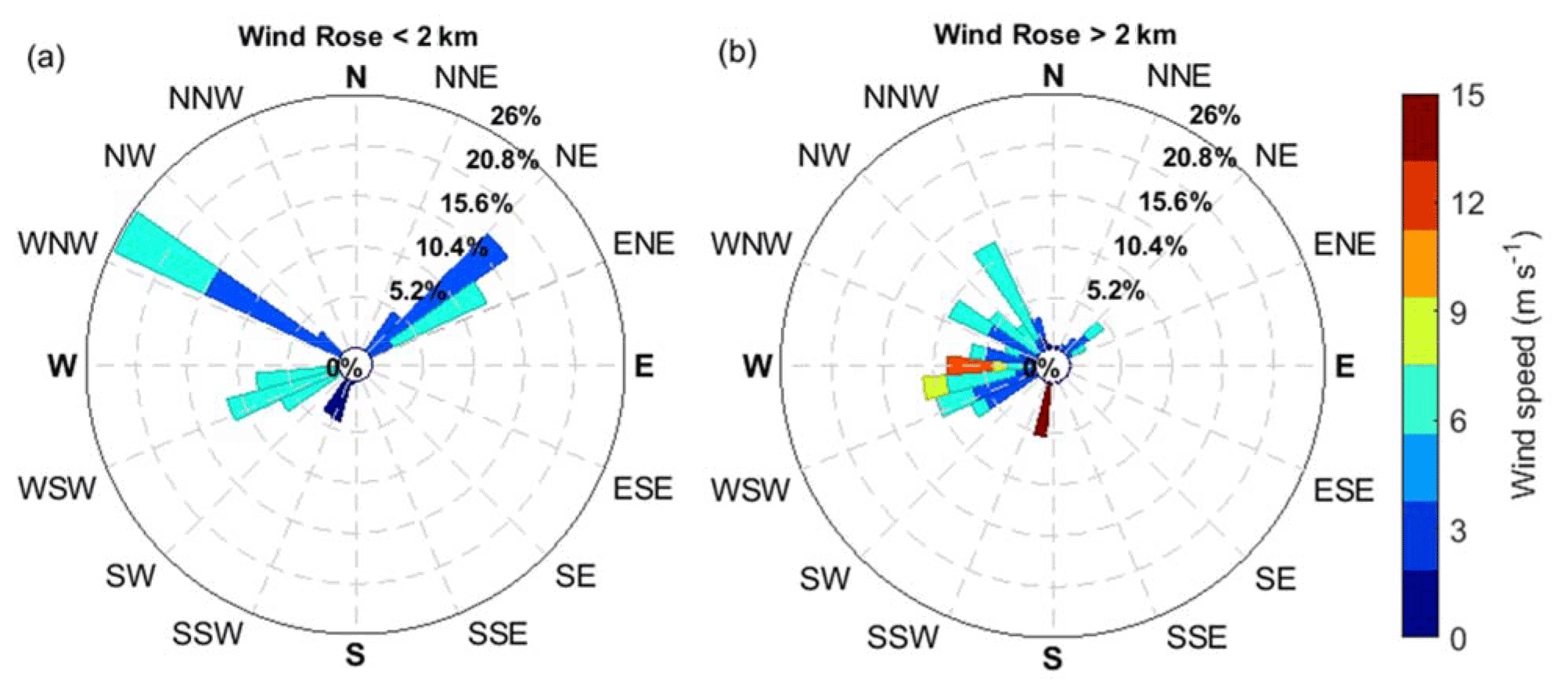
Figure 4 Wind rose (a) below 2 km (8 cases) and (b) above 2 km (24 cases) from radiosoundings measurements in Barcelona. The colorbar on the right applies to both plots.

For both wind roses, the most frequent wind speeds reach around 6 m s⁻¹ designated as a moderate breeze (World Meteorological Organization and Global Atmosphere Watch, 2003). This low wind speed maintains a good homogeneity of the atmospheric aerosols in the selected layers, i.e., a constant mixture of aerosols over time.

Figure 5a and e show the resulting spectral Hänel fits at both height levels. Figure 5b–d and f–h show all enhancement factors per wavelength below and above 2 km a.g.l., respectively. In all those plots, the Hänel fits (solid lines) are calculated with the mean hygroscopic growth parameter $\stackrel{\mathrm{‾}}{\mathit{\gamma }}(\mathit{\lambda }$) of all individuals γ(λ), and the variability associated with them (colored shaded area) is calculated taking into account the standard deviation of all individual γ(λ). The enhancement factors and Hänel fits in Fig. 5 are those scaled in order to start at RH_ref= 40 %. The spectral values of $f_{\mathrm{ref}}^{\mathit{\lambda }}\left(\mathrm{RH}=\mathrm{85}\mathit{\%}\right)$ and $\stackrel{\mathrm{‾}}{\mathit{\gamma }}(\mathit{\lambda }$) at both height levels are reported in Table 2, which also includes the mean of the correlation coefficients, R², of the individual pairs of (β^λ, RH), as well as the average of the layer-mean Ångström exponents, ${\mathrm{AE}}_{{\mathit{\lambda }}_{\mathrm{1}},{\mathit{\lambda }}_{\mathrm{2}}}$, between the pairs of wavelengths (355, 532 nm and 532, 1064 nm). The first result to comment is that, independently of the height level, the correlation coefficients of the individual fits are high (> 0.91) and present a small fluctuation (σ < 0.06, except for λ= 355 nm and above 2 km where σ= 0.14). These high values of R² indicate the good correlation that exists between the profiles of the backscatter coefficients and the profiles of the RH in the selected layer.

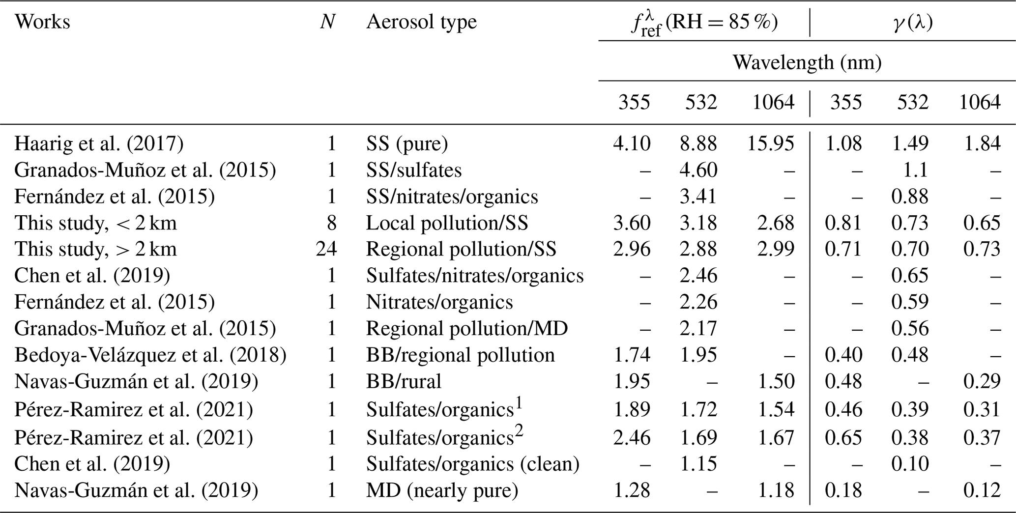
Below 2 km, the particle backscatter coefficient enhancement factor seems to have a clear spectral behavior: $f_{\mathrm{ref}}^{\mathit{\lambda }}\left(\mathrm{RH}=\mathrm{85}\mathit{\%}\right)$ (γ(λ)) is 3.60 ± 2.47 (0.81 ± 0.41), 3.18 ± 2.07 (0.73 ± 0.40) and 2.68 ± 1.20 (0.65 ± 0.31) at 355, 532 and 1064 nm, respectively. This behavior (decrease of $f_{\mathrm{ref}}^{\mathit{\lambda }}\left(\mathrm{RH}=\mathrm{85}\mathit{\%}\right)$ or γ(λ) with increasing wavelength) implies that the water uptake by the particles modifies the particle backscatter coefficient more strongly at shorter wavelengths than at larger wavelengths. Since the 355 nm wavelength is sensitive to smaller aerosols compared to larger wavelengths, larger fit coefficients at 355 nm indicate slightly more hygroscopic aerosols present at smaller size ranges (Zieger et al., 2013; Dawson et al., 2020): AE_355,532 and AE_532,1064 are 1.07 and 0.93, respectively. Although quite similar, the difference between both AE${}_{{\mathit{\lambda }}_{\mathrm{1}},{\mathit{\lambda }}_{\mathrm{2}}}$ also points out a spectral sensitivity of the backscatter coefficient slightly larger at shorter wavelengths than at larger ones. Note en passant that our Ångström exponent values are in the range of column-averaged monthly values found by Sicard et al. (2011) and estimated from a long-term lidar database in Barcelona. Next, we aim to compare our results with the literature. The hygroscopic growth parameter γ depends on neither RH_min, nor RH_max, so the values of γ from the literature can be compared directly to ours. Contrarily, the f values depend strongly on RH_min and RH_max, so for the literature to be comparable with our values, the hygroscopic growth parameter γ from the literature is used to calculate $f_{\mathrm{ref}}^{\mathit{\lambda }}\left(\mathrm{RH}=\mathrm{85}\mathit{\%}\right)$ with RH_ref= 40 %. Also, we have only considered works in which the enhancement factor was calculated for the backscatter coefficient measured with a lidar. Works in which the enhancement factor was calculated for the extinction coefficient (Veselovskii et al., 2009; Dawson et al., 2020) or from in situ data (Carrico et al., 2003; Titos et al., 2016; Skupin et al., 2016; among others) are not considered for comparison with our study. The literature results are summarized in Table 3 and represented in Fig. 6 in terms of $f_{\mathrm{ref}}^{\mathit{\lambda }}\left(\mathrm{RH}=\mathrm{85}\mathit{\%}\right)$ and γ(λ). The values in Table 3 are ordered from high to low values of $f_{\mathrm{ref}}^{\mathrm{532}}\left(\mathrm{RH}=\mathrm{85}\mathit{\%}\right)$ or γ(532 nm), and, very interestingly, a natural classification of the dominating aerosol regime, underlined by a color code in Fig. 6, appears. The highest values of $f_{\mathrm{ref}}^{\mathrm{532}}\left(\mathrm{RH}=\mathrm{85}\mathit{\%}\right)$ (> 3) all represent situations with a notable fraction of sea salt; values of $f_{\mathrm{ref}}^{\mathrm{532}}\left(\mathrm{RH}=\mathrm{85}\mathit{\%}\right)$ between 2 and 3 are representative of polluted situations with different mixtures; near the value of 2 we find biomass burning; between 1.5 and 2 rural background with automobile traffic; and values of $f_{\mathrm{ref}}^{\mathrm{532}}\left(\mathrm{RH}=\mathrm{85}\mathit{\%}\right)$ close to 1 correspond to clean and mineral dust cases. Despite the small statistics of this analysis, the fact that these measurements made in different places of the Earth and in different aerosol loads lead to a coherent classification when put all together gives a certain credit to the analysis. It is also corroborated by a certain number of works. Haarig et al. (2017) precisely evaluated the hygroscopic growth of pure sea salt in Barbados and established the top limit presented here ($f_{\mathrm{ref}}^{\mathrm{532}}\left(\mathrm{RH}=\mathrm{85}\mathit{\%}\right)=$ 8.88). Chen et al. (2019) established that the aerosol hygroscopicity in large cities (pollution) is driven by the hygroscopicity of inorganics emitted essentially by the vehicular transport (nitrates, sulfates and ammonium) and water-soluble organic carbonaceous particles. Based on Liu et al. (2014), the following components have a decreasing hygroscopicity: sulfate acid is the most hygroscopic, followed by nitrates, sulfates and water-soluble organics. The hygroscopicity (γ) of smoke particles dominated by carbonaceous organic material from biomass burning has been evaluated by Gomez et al. (2018) to not be larger than 0.4 (equivalent to $f_{\mathrm{ref}}^{\mathrm{532}}\left(\mathrm{RH}=\mathrm{85}\mathit{\%}\right)$ < 1.74). Finally, relatively clean aerosols and mineral dust were estimated to be poorly hygroscopic by Chen et al. (2019) and Navas-Guzmán et al. (2019), respectively. All these results from independent studies are consistent with the classification presented in this paper. The singular spectral behavior of $f_{\mathrm{ref}}^{\mathit{\lambda }}\left(\mathrm{RH}=\mathrm{85}\mathit{\%}\right)$ or γ(λ) observed in our study below 2 km was reported, although with smaller values, between 355 and 1064 nm for a mixture of biomass burning and rural aerosols by Navas-Guzmán et al. (2019) and between 355, 532 and 1064 nm for sulfates and organics by Pérez-Ramírez et al. (2021). Given the little literature on the subject, it is difficult to attribute the decrease of $f_{\mathrm{ref}}^{\mathit{\lambda }}\left(\mathrm{RH}=\mathrm{85}\mathit{\%}\right)$ with increasing wavelengths to one type of aerosol or another at this point. However, the quantitative difference observed between our study (2.68 < $f_{\mathrm{ref}}^{\mathit{\lambda }}\left(\mathrm{RH}=\mathrm{85}\mathit{\%}\right)$ < 3.60), Navas-Guzmán et al. (2019) and Pérez-Ramírez et al. (2021) (1.50 < $f_{\mathrm{ref}}^{\mathit{\lambda }}\left(\mathrm{RH}=\mathrm{85}\mathit{\%}\right)$ < 1.95) is most probably due to the presence of marine aerosols in our study which are present in neither Switzerland (Navas-Guzmán et al., 2019) nor Baltimore–Washington (Pérez-Ramírez et al., 2021). The presence of marine aerosols in Barcelona also explains why higher $f_{\mathrm{ref}}^{\mathit{\lambda }}\left(\mathrm{RH}=\mathrm{85}\mathit{\%}\right)$ are found compared to the rest of the studies also dominated by pollution (Fernández et al., 2015; Granados-Muñoz et al., 2015; Chen et al., 2019) in which the presence of marine aerosols is not mentioned.

Figure 5 Particle backscatter coefficient enhancement factors with RH_ref= 40 % at 355, 532, and 1064 nm. (a) Spectral Hänel fits for the cases below 2 km at 355, 532, and 1064 nm; (b) individual $f_{\mathrm{ref}}^{\mathrm{355}}$ and mean Hänel fit; (c) individual $f_{\mathrm{ref}}^{\mathrm{532}}$ and mean Hänel fit; (d) individual $f_{\mathrm{ref}}^{\mathrm{1064}}$ and mean Hänel fit; (e–h) same as (a–d) for the cases above 2 km. The shaded areas around the mean Hänel fits represent the standard deviation of all individual fits.

Table 2 Spectral enhancement factor $f_{\mathrm{ref}}^{\mathit{\lambda }}$ at RH= 85 % and RH_ref= 40 %. Mean and standard deviation (σ) of γ(λ) and the correlation coefficient, R². Results are given separately for hygroscopic layers (the layers where hygroscopic growth was calculated) below and above 2 km. The layer-mean Ångström exponent between the pairs (355, 532 nm) and (532, 1064 nm) is reported in the last two columns.

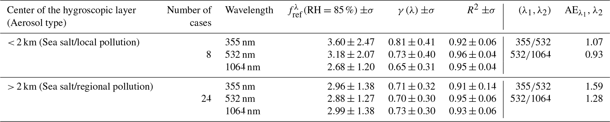
Table 3 $f_{\mathrm{ref}}^{\mathit{\lambda }}$ at RH= 85 % and RH_ref= 40 % and γ(λ) from the literature and from this study (in bold font). Values are listed in a decreasing order of the values at λ= 532 nm. SS stands for sea salt, MD for mineral dust and BB for biomass burning. N is the number of cases. Organics¹ indicates a greater amount of organics compared to Organics².

Above 2 km, the particle backscatter coefficient enhancement factor seems to have no spectral dependency: $f_{\mathrm{ref}}^{\mathit{\lambda }}\left(\mathrm{RH}=\mathrm{85}\mathit{\%}\right)$ (γ(λ)) is 2.96 ± 1.38 (0.71 ± 0.32), 2.88 ± 1.27 (0.70 ± 0.30) and 2.99 ± 1.38 (0.73 ± 0.30) at 355, 532 and 1064 nm, respectively. Such a flat spectral dependency has only been observed by Navas-Guzmán et al. (2019) between 355 and 1064 nm for mineral dust. We believe that the spectral dependency of the total aerosol content is a function of the chemical composition and of the concentration of each one of the hygroscopic components, and for this reason it is highly variable. Although the hygroscopic parameter of relevant particle components has been reviewed by Liu et al. (2014), our conclusion calls for further chemical analysis and laboratory studies to determine the spectral behavior of these relevant particles.

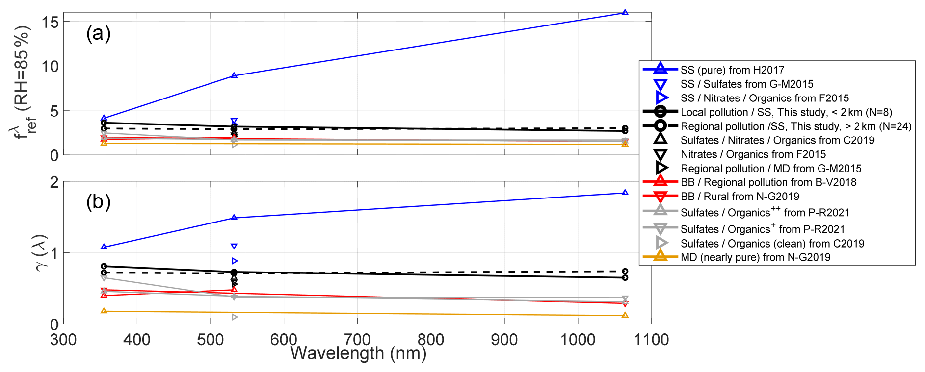
Figure 6 (a) $f_{\mathrm{ref}}^{\mathit{\lambda }}$ at RH= 85 % and RH_ref= 40 % and (b) γ(λ) from the literature and from this study as a function of wavelength. Colored symbols represent the dominating regime: blue for sea salt, black for pollution, red for biomass burning, grey for traffic + rural and clean, and orange for mineral dust. The references are Haarig et al. (2017) (H2017), Granados-Muñoz et al. (2015) (M-G2015), Fernández et al. (2015) (F2015), Chen et al. (2019) (C2019), Bedoya-Velásquez et al. (2018) (B-V2018), Navas-Guzmán et al. (2019) (N-G2019) and Pérez-Ramírez et al. (2021) (P-R2021). Organics${}^{++}$ indicates a greater amount of organics compared to Organics⁺.

3.2 Climatological analysis at 532 nm

In this section we present, for the first time, a climatological analysis of the aerosol hygroscopic growth observed along a vertical range in ambient conditions by means of the hygroscopic growth parameter, γ(λ), and the particle backscatter coefficient enhancement factor at RH = 85 %, $f_{\mathrm{ref}}^{\mathit{\lambda }}\left(\mathrm{RH}=\mathrm{85}\mathit{\%}\right)$. Data from both the multi-wavelength ACTRIS/EARLINET lidar (period 2010–2018) and the MPL (period 2015–2018) are considered. The common wavelength is λ= 532 nm. All data were screened according to the selection criteria mentioned in Sect. 2.2. As in Sect. 3.1, all cases associated with a mineral dust intrusion are not included in this study. We find a total of 76 cases distributed along all months of the year. The monthly variation of γ(532) is represented in Fig. 7. The mean-layer height (MLH) and mean-layer relative humidity (MLRH) calculated as the mean value in the hygroscopic layer (the layer where hygroscopic growth was calculated) of the height and RH, respectively, are also plotted. The seasonal means of γ(532), MLH and MLRH are reported in Table 4. Winter includes the months of December, January and February; spring includes March, April and May; summer includes June, July and August; and autumn includes September, October and November.

From the top plot of Fig. 7, one sees that the aerosol hygroscopic growth parameter is on average rather constant all year round. However, for each single month, large standard deviations of γ(532) are observed (red shaded area in Fig. 7), which indicate the presence of aerosols with different hygroscopic properties all year round. The annual mean of γ(532) is 0.55. While the seasonal deviations from that mean are small ($\le \pm$ 0.03, Table 4), the standard deviations associated with each season are large (they vary between ±0.21 and ±0.25). The annual mean of the enhancement factor at RH= 85 %, $f_{\mathrm{ref}}^{\mathrm{532}}\left(\mathrm{RH}=\mathrm{85}\mathit{\%}\right)$, is 2.26 ± 0.72 and the seasonal deviations from that mean are not larger than ±0.08. Unlike γ(532), the MLH shows an annual cycle: the hygroscopic layers are detected at the highest height in summer (summer MLH = 2.40 ± 1.13 km) and at the lowest height in winter (winter MLH = 1.19 ± 0.66 km). With regard to former works of Sicard et al. (2006) establishing that the PBL in Barcelona is not significantly different between winter and summer seasons, and that it is usually lower than 1.0 km, our findings suggest that hygroscopic layers in autumn (MLH = 1.31 km) and winter (MLH = 1.19 km) are detected near the top or slightly above the climatological mean PBL height, and clearly above the PBL in spring (MLH = 1.81 km) and summer (MLH = 2.40 km). Although the hygroscopic aerosols are detected above the PBL in spring and summer, they might not be that different from the aerosols in the PBL. Indeed Pérez et al. (2004) showed that in Barcelona the combined effects of strong insolation, weak synoptic forcing, sea breezes and mountain-induced winds create recirculations of pollutants injected at various heights above the PBL and up to 4.0 km. Like γ(532), the MLRH is also rather constant all year round, which confirms that aerosol hygroscopic properties are not related to the level of humidity in the atmosphere. The annual mean, ∼70 %, is close to the annual average (72 %) at ground level (Weather and Climate, 2021), which is higher than most other Spanish cities because of the presence of the sea in Barcelona. The comparison with the literature is not straightforward due to the lack of studies of long-term datasets. Sheridan et al. (2001) and Jefferson et al. (2017) analyzed 1 and 7 years, respectively, of aerosol growth factors retrieved from scattering coefficients at 550 nm, measured with humidified nephelometers in an agricultural region of Southern Great Plains in the United States, a completely different site from Barcelona in terms of aerosol composition (aged aerosols of mostly organic composition vs. anthropogenic, crustal and marine aerosols). Even if the findings of Jefferson et al. (2017) are based on scattering-derived (and not backscattering) hygroscopic growth parameters, some differences and similarities with our study are worth mentioning:

• The annual mean of γ is 0.40, much lower than in our study (0.55) where the effect of sea salt is noticeable.

• The annual standard deviation of γ is 0.15, proportionally similar to σ= 0.23 found in our study.

• γ is higher in winter (higher nitrate mass fraction) and lower in summer (higher organic mass fraction), whereas it is not season-dependent in our study.

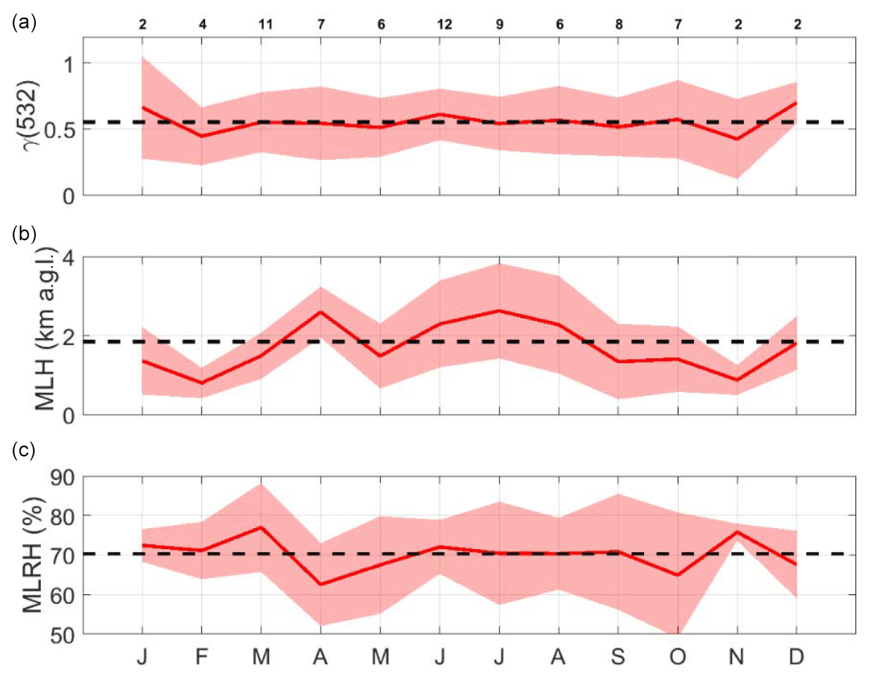
Figure 7 Monthly (a) hygroscopic growth parameter at 532 nm, γ(532); (b) mean-layer height (MLH); (c) mean-layer relative humidity (MLRH). The red shaded area represents the standard deviation. The yearly average is represented with a black dash line. The numbers above the top plot are the number of hygroscopic cases per month.

An interesting result from Jefferson et al. (2017), complementary to our analysis, is the retrieval of γ for sub-1 and sub-10 µm particles for which the annual mean is 0.44 and 0.40, respectively. The lower sub-10 µm values of γ are attributed to the influence from soil dust.

Table 4 Seasonal and yearly mean and standard deviation (σ) of $f_{\mathrm{ref}}^{\mathrm{532}}$ at RH = 85 % and RH_ref= 40 %, γ(532), the mean layer height (MLH) and the mean-layer relative humidity (MLRH). N is the number of hygroscopic cases. The yearly means are also given for the cases No cloud and Below-cloud.

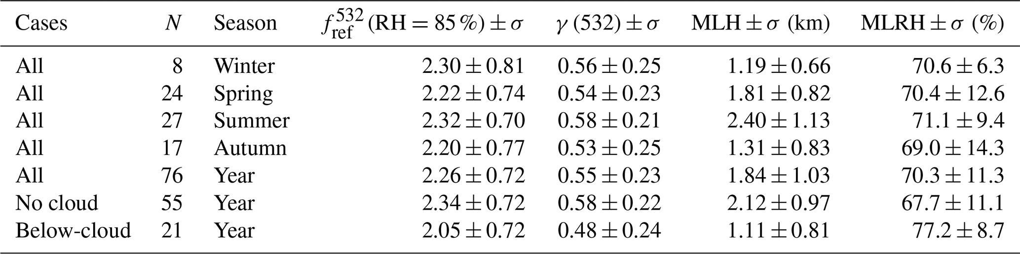
Our search for a special dependency of the hygroscopic growth with other factors (layer height, day/night, level of humidity, etc.) was rather unfruitful. However, by looking at all 76 cases individually, and in particular at the vertical profiles of the backscatter coefficient and RH, we found a possible subcategorization into 2 classes: cases with no cloud in the vertical range examined (referred hereafter as No cloud) and cases where the hygroscopic behavior was detected just below a cloud (referred hereafter as Below-cloud). From the whole dataset, 55 cases were classified as No cloud and 21 as Below-cloud. We have checked that all cases were in subsaturation humidity conditions (RH < 100 %, the water is in vapor form and the aerosol cannot activate (yet) into a droplet). Figure 8 shows examples of both cases. The annual means of γ(532), $f_{\mathrm{ref}}^{\mathrm{532}}\left(\mathrm{RH}=\mathrm{85}\mathit{\%}\right)$, MLH and MLRH for both cases are also reported in the bottom part of Table 4. On a yearly basis the Below-cloud cases have a lower γ(532) (0.48 vs. 0.58 for the No cloud cases), which occur at a lower altitude (MLH = 1.11 km vs. 2.12 km) and at a higher RH (MLRH = 77.2 % vs. 67.7 %). The Below-cloud cases occur inside or near the top of the PBL where the formation of convective non-precipitating PBL clouds is frequent in coastal sites (Papayannis et al., 2017). In such cases, the RH is higher than in the No cloud cases. The aerosol below the cloud starts to activate as cloud condensation nuclei (CCN). Its size grows through adsorption of water vapor, its scattering properties increase, and as the aerosol size grows, its potential to keep growing is reduced compared to a drier aerosol. All of this is well illustrated in the two cases shown in Fig. 8: while both the backscatter coefficient and the RH are low (RH < 55 %, β⁵³² < 1 Mm⁻¹ sr⁻¹) in the absence of clouds (Fig. 8a), they are high (RH > 80 %, β⁵³² > 2 Mm⁻¹ sr⁻¹) and increase strongly with height in the Below-cloud case (Fig. 8b). So, although one would be tempted to visually attribute the strongest growth to the Below-cloud case, in practice the contrary occurs: γ(532) is higher for No cloud (0.87) than for Below-cloud (0.53). The same result is reflected in the climatological data (Table 4): γ(532)= 0.58 for No cloud and 0.48 for Below-cloud. There are at least three reasons for this:

• The first reason has been given above: the aerosol activation as CCN in high humidity conditions reduces its potential to keep growing compared to the aerosol in drier conditions.

• The second one is mathematical, definition-dependent and inherent to the aerosol composition. According to the definition of the enhancement factor (Eq. 3), defined as a power law function normalized to a RH_ref of 40 %, one sees that (bottom plots of Fig. 8): (1) in cases with low RH, $f_{\mathrm{ref}}^{\mathrm{532}}$ varies very little and a relatively high γ(532) is required to provoke departure of $f_{\mathrm{ref}}^{\mathrm{532}}$ from unity; and (2) for high RH cases, $f_{\mathrm{ref}}^{\mathrm{532}}$ varies steeply and a relatively low γ(532) is enough to provoke strong variations of $f_{\mathrm{ref}}^{\mathrm{532}}$.

• The third explanation is linked to the specific aerosol composition at the site. In Fig. 9 we show box and whisker plots of the percentiles of the seasonal values of γ(532) for all cases, and for the No cloud and Below-cloud cases. When considering all cases, the results for the monthly statistics are reproduced for the seasonal one: γ(532) is not season-dependent. In spring and summer, γ(532) for No cloud is not significantly different from γ(532) for all cases; for Below-cloud γ(532) is slightly larger but well within the seasonal standard deviation (see Table 4). The most important difference is in autumn when the mean γ(532) is 0.71 for No cloud and 0.33 for Below-cloud, i.e., respectively well above and below the autumn mean of all cases (0.53).

This last paragraph presents a discussion on the possible explanations of the difference observed in autumn in Fig. 9, which may rely on the concomitance of several factors. As far as the No cloud cases are concerned, in Barcelona hydrophilic inorganics such as nitrates (the most abundant) and ammonium are maximum in autumn and winter, while sulfates are minimum (Querol et al., 2001). The persistence of anticyclonic stagnating conditions during these seasons favor the accumulation of the pollutants in the PBL (Querol et al., 2001; Pey et al., 2010). In such conditions more pollutants are prone to convective vertical motion and activation as CCN if high humidity conditions are also present. Gunthe et al. (2011) showed that aged pollution particles in stagnant air (soluble inorganics dominate the mass fraction) are on average larger and more hygroscopic than fresh pollution particles (organics and elemental carbon dominate the mass fraction). Taken all together, these results support the higher values of γ(532) for the No cloud cases found in autumn (0.71) compared to the rest of the year (0.52–0.60). Two things in Fig. 9 remain to be elucidated: why the hygroscopicity of the Below-cloud cases is lower in autumn than during the rest of the year and why it is lower than that of the No cloud cases during the same season. These questions are difficult to answer without complementary in situ measurements, and at this point, only a hypothesis can be formulated. The seasonal statistics available indicate that the mean-layer backscatter coefficient (not shown) in the hygroscopic layer of the Below-cloud cases is larger in autumn (1.71 Mm⁻¹ sr⁻¹) than in spring (0.73 Mm⁻¹ sr⁻¹) and summer (1.35 Mm⁻¹ sr⁻¹); the same occurs for the MLRH, but to a lesser extent (79.7 % in autumn vs. 74.3 % and 76.5 % in spring and summer, respectively); and the opposite for the MLH (0.60 km – i.e., within the PBL, see Sicard et al. (2006) – in autumn vs. 1.29 and 1.64 km – i.e., above the PBL – in spring and summer, respectively). Thus, in autumn the Below-cloud hygroscopic layers are within the PBL; hence the larger β⁵³² is observed with respect to the spring and summer seasons. The lower autumn γ(532) could reflect a higher fraction of organics in the aerosol mixture in the PBL in autumn vs. a higher amount of inorganics in the aerosol mixture above the PBL in spring and summer (possibly coming from the recirculation of pollutants injected at various heights above the PBL (see Pérez et al. 2004)). Note that this statement is a pure hypothesis. The literature emphasizes the complexity of the atmospheric aerosol hygroscopicity linked to their highly variable composition and chemical transformation. Cheung et al. (2020) suggest that the uptake of hydrophilic/hydrophobic species during particle growth and coagulation processes may influence the hygroscopicity of aerosols. Cruz and Pandis (2000) study the effect of organic mixing and coating on the hygroscopic behavior of inorganics and on NaCl particles in particular. Interestingly, they find that, depending on the organic mass fraction, the NaCl–organic mixtures could not only decrease (down to 40%), but also increase (up to 20 %) the hygroscopicity of the mixture. More recently Ruehl and Wilson (2014) emphasized the new and complex relationship between the composition of an organic aerosol and its hygroscopicity and in the same field Liu et al. (2018) study some of the microphysical mechanisms involved in the hygroscopicity of secondary organic material in the laboratory. All studies call for further laboratory and field research. The difference between the autumn Below-cloud (0.33) γ(532) and No cloud (0.71) is significant. The mean-layer backscatter coefficient in the hygroscopic layer of the Below-cloud (1.71 Mm⁻¹ sr⁻¹) is approximately twice as large than the No cloud cases (0.80 Mm⁻¹ sr⁻¹). The autumn MLRH/MLH are higher/lower for the Below-cloud (79.7 %/0.60 km) than for the No cloud cases (59.5 %/1.93 km). It is possible here again to hypothesize that the lower γ(532) for Below-cloud could reflect a higher fraction of organics in the aerosol mixture in the PBL with higher humidity conditions vs. a higher amount of inorganics in the aerosol mixture in the free troposphere in the No cloud cases. Note that this statement is again a pure hypothesis. In summary, the observations in autumn show that the Below-cloud aerosols are detected in the PBL, at high RHs, and have large backscatter coefficients and low hygroscopic growth parameters. We close this section with a question: may the activation into CCN at the base of the cloud be affecting inorganic salts predominantly and thus generating a depletion of them and leave room to an organic-rich layer below the cloud?

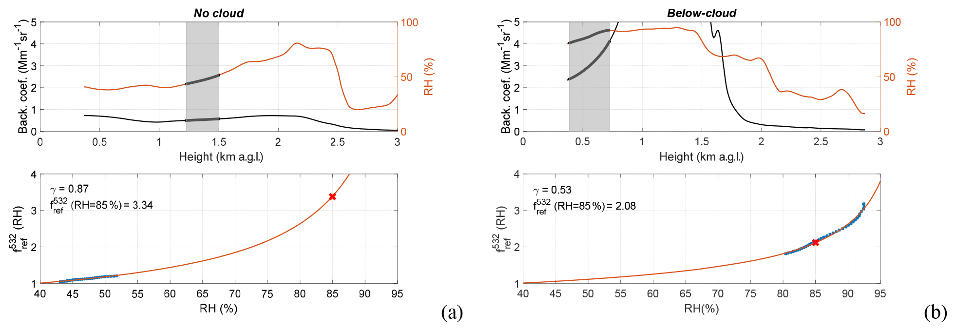
Figure 8 (a) No cloud and (b) Below-cloud cases; (top) backscatter coefficient (black, left axis) and relative humidity (red, right axis) versus height; (bottom) $f_{\mathrm{ref}}^{\mathrm{532}}$ at RH= 85 % and RH_ref= 40 % (blue crosses) and Hänel fit (red line). In the top plots the hygroscopic layer is reported in a shaded rectangle and thicker lines.

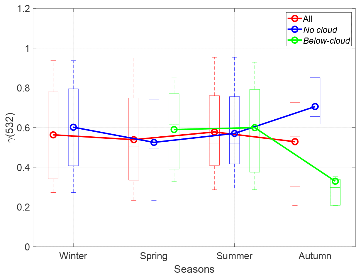
Figure 9 Box and whisker plot showing the 5, 25, 50, 75, and 95th percentiles of the seasonal values of γ(532) for all cases (red), and the No cloud (blue) and Below-cloud cases (green). Circles indicate the arithmetic mean. Seasonal percentiles and means are shown only when more than one data point is available.

4 Conclusions

A spectral and climatological analysis of the aerosol hygroscopic growth parameter observed in the atmospheric vertical column combining lidar and radiosounding measurements is presented. The hygroscopic cases have been selected by filtering time coincident lidar and radiosounding measurements, by detecting coincident backscatter coefficient and RH increases with increasing height, and by limiting the variations of variables used as indicators of well mixed conditions such as WVMR, potential temperature, and wind speed and direction. Results are presented in terms of the hygroscopic growth parameter, γ, which is the result of fitting the particle backscatter coefficient enhancement factor with the Hänel parameterization and the particle backscatter coefficient enhancement factor, f_ref(RH=85 %), at RH = 85 % with RH_ref= 40 %. For our results to be comparable with the literature giving enhancement factors for a large variety of RH_ref and RH_max, a very simple conversion for any values of RH_ref $/$ RH_max is proposed and applied to the literature values to get f_ref(RH=85 %) with RH_ref= 40 %.

The spectral analysis performed at the wavelengths of 355, 532 and 1064 nm distinguishes aerosols in layers below 2 km (regime of local pollution and sea salt) and above 2 km (regime of regional pollution and residual sea salt). Below 2 km, γ decreases with increasing wavelengths (γ= 0.81, 0.73 and 0.65; $f_{\mathrm{ref}}^{\mathit{\lambda }}\left(\mathrm{RH}=\mathrm{85}\mathit{\%}\right)=$ 3.60, 3.18 and 2.68). Since the 355 nm wavelength is sensitive to smaller aerosols, this behavior could indicate slightly more hygroscopic aerosols present at smaller size ranges. This hypothesis is supported by the Ångström exponents which are higher for the pair (355, 532) than for (532, 1064), which points out a spectral sensitivity of the backscatter coefficient slightly larger at shorter wavelengths than at larger wavelengths. Above 2 km the values of γ (0.71, 0.70 and 0.73; $f_{\mathrm{ref}}^{\mathit{\lambda }}\left(\mathrm{RH}=\mathrm{85}\mathit{\%}\right)=$ 2.96, 2.88 and 2.99) are comparable to those below 2 km, and their spectral behavior is flat. This analysis and others from the literature are put together in a table presenting, for the first time spectrally, the hygroscopic growth parameter and enhancement factors of a large variety of atmospheric aerosol hygroscopicities going from low (pure mineral dust, γ < 0.2; $f_{\mathrm{ref}}^{\mathit{\lambda }}\left(\mathrm{RH}=\mathrm{85}\mathit{\%}\right)$ < 1.3) to high (pure sea salt, γ > 1.0; $f_{\mathrm{ref}}^{\mathit{\lambda }}\left(\mathrm{RH}=\mathrm{85}\mathit{\%}\right)$ > 4.0). In this table, the highest values of $f_{\mathrm{ref}}^{\mathrm{532}}\left(\mathrm{RH}=\mathrm{85}\mathit{\%}\right)$ (> 3) all represent situations with a notable fraction of sea salt; values of $f_{\mathrm{ref}}^{\mathrm{532}}\left(\mathrm{RH}=\mathrm{85}\mathit{\%}\right)$ between 2 and 3 are representative of polluted situations with different mixtures; near the value of 2 we find biomass burning; between 1.5 and 2 rural background with automobile traffic; and values of $f_{\mathrm{ref}}^{\mathrm{532}}\left(\mathrm{RH}=\mathrm{85}\mathit{\%}\right)$ close to 1 correspond to clean and mineral dust cases.

The climatological analysis shows that γ at 532 nm is rather constant all year round and has a large monthly standard deviation, suggesting the presence of aerosols with different hygroscopic properties all year round. The annual γ is 0.55 ± 0.23 ($f_{\mathrm{ref}}^{\mathrm{532}}\left(\mathrm{RH}=\mathrm{85}\mathit{\%}\right)=$2.26 ± 0.72). The height of the hygroscopic layers shows an annual cycle with a maximum clearly above the PBL in summer and a minimum near the top of the PBL in winter. Although the hygroscopic aerosols are detected above the PBL in spring and summer, they might not be that different from the aerosols in the PBL. Former works describing the presence of recirculation layers of pollutants injected at various heights above the PBL may explain why γ, unlike the height of the hygroscopic layers, is not season-dependent. The subcategorization of the whole database into No cloud and Below-cloud cases reveals a large difference of γ in autumn between both categories (0.71 and 0.33, respectively), possibly attributed to a depletion of inorganics at the point of activation into CCN in the Below-cloud cases. Our work calls for more in situ measurements to synergetically complete studies, like this one, based mostly on remote sensing measurements.