Potential environmental impact of bromoform from Asparagopsis farming in Australia

To mitigate the rumen enteric methane (CH₄) produced by ruminant livestock, Asparagopsis taxiformis is proposed as an additive to ruminant feed. During the cultivation of Asparagopsis taxiformis in the sea or in terrestrially based systems, this macroalgae, like most seaweeds and phytoplankton, produces a large amount of bromoform (CHBr₃), which contributes to ozone depletion once released into the atmosphere. In this study, we focus on the impact of CHBr₃ on the stratospheric ozone layer resulting from potential emissions from proposed Asparagopsis cultivation in Australia. The impact is assessed by weighting the emissions of CHBr₃ with its ozone depletion potential (ODP), which is traditionally defined for long-lived halocarbons but has also been applied to very short-lived substances (VSLSs). An annual yield of ∼3.5 × 10⁴ Mg dry weight is required to meet the needs of 50 % of the beef feedlot and dairy cattle in Australia. Our study shows that the intensity and impact of CHBr₃ emissions vary, depending on location and cultivation scenarios. Of the proposed locations, tropical farms near the Darwin region are associated with the largest CHBr₃ ODP values. However, farming of Asparagopsis using either ocean or terrestrial cultivation systems at any of the proposed locations does not have the potential to significantly impact the ozone layer. Even if all Asparagopsis farming were performed in Darwin, the CHBr₃ emitted into the atmosphere would amount to less than 0.02 % of the global ODP-weighted emissions. The impact of remaining farming scenarios is also relatively small even if the intended annual yield in Darwin is scaled by a factor of 30 to meet the global requirements, which will increase the global ODP-weighted emissions up to ∼0.5 %.

1 Introduction

Livestock is responsible for about 15 % of total anthropogenic greenhouse gas (GHG) emissions weighted by radiative forcing (Gerber et al., 2013), ranking it amongst the main contributors to climate change. The global demand for red meat and dairy is expected to increase >50 % by 2050 compared to the 2010 level; thus mitigation measures to reduce the GHG emissions from the global livestock industry are in high demand (Beauchemin et al., 2020). Total GHG emissions (e.g., CH₄) from ruminant livestock contribute about 18 % of the total global carbon dioxide equivalent (CO₂-eq) inventory (Herrero and Thornton, 2013). With a global warming potential ∼30 times higher than carbon dioxide (CO₂) and a much shorter lifetime (∼10 years, IPCC, 2021), ruminant enteric CH₄ is an attractive and feasible target for global warming mitigation.

Enteric CH₄ from ruminant livestock is produced and released into the atmosphere through rumen microbial methanogenesis (Morgavi et al., 2010). Methanogenic archaea (methanogens) intercept substrate CO₂ and H₂ liberated during bacterial fermentation of feed materials (Kamra, 2005), and during this inefficient digestion process (Herrero and Thornton, 2013; Patra, 2012), methanogen metabolism leads to reductive CH₄ production and loss of feed energy as CH₄ emissions. To abate enteric methanogenesis, different strategies such as feeding management and antimethanogenic feed ingredients have been proposed and assessed (e.g., Moate et al., 2016; Mayberry et al., 2019; Beauchemin et al., 2020). Some types of macroalgae have been demonstrated to mitigate production of CH₄ during in vitro and in vivo rumen fermentation significantly (Machado et al., 2014; Kinley and Fredeen 2015; Li et al., 2018; Kinley et al., 2020; Abbott et al., 2020). Among the different macroalgae species, Kinley et al. (2016a) concluded that the red algae Asparagopsis spp. showed the most potential for reducing CH₄ production. Kinley et al. (2016b) further demonstrated that forage with the addition of 2 % Asparagopsis taxiformis could eliminate CH₄ production in vitro without negative effects on forage digestibility. In recent animal experiments, reduction of enteric CH₄ production by more than 98 % was achieved with only 0.2 % addition of freeze-dried and milled Asparagopsis taxiformis to the organic matter (OM) content of feedlot cattle feed (Kinley et al., 2020).

Halogenated, biologically active secondary metabolites are pivotal in the reduction of CH₄ induced by Asparagopsis (Abbott et al., 2020). Most of the reduction is ascribed to bromoform (CHBr₃) inhibition of the CH₄ biosynthetic pathway within methanogens (Machado et al., 2016). CHBr₃ as a natural halogenated volatile organic compound originates from chemical and biological sources including marine phytoplankton and macroalgae (Carpenter and Liss, 2000; Quack and Wallace, 2003). When emitted to the atmosphere, CHBr₃ has an atmospheric lifetime shorter than 6 months and is often referred to as a very short-lived substance (VSLS). Once released into the atmosphere, degraded halogenated VSLSs can catalytically destroy ozone in the troposphere and stratosphere, thus drawing them considerable interest (Engel et al., 2018; Zhang et al., 2020). Bromoform is the dominant compound among bromine-containing VSLS emissions, resulting mostly from natural sources (Quack and Wallace, 2003) and to a lesser degree from anthropogenic production (Maas et al., 2019, 2021). With an atmospheric lifetime of about 17 d (Carpenter et al., 2014), CHBr₃ can deliver bromine to the stratosphere under appropriate conditions of emission strength and vertical transport (e.g., Aschmann et al., 2009; Liang et al., 2010; Tegtmeier et al., 2015, 2020) and thus contribute to ozone depletion in the lower and middle stratosphere (e.g., Yang et al., 2014; Sinnhuber and Meul, 2015). Global research on enabling large-scale seaweed Asparagopsis farming is increasing (Black et al., 2021) as it appears to be one of the most promising options as an antimethanogenic feed ingredient to achieve carbon neutrality in the livestock sector within the next decade (Kinley et al., 2020; Roque et al., 2021). In consequence, the environmental impact of CHBr₃ due to Asparagopsis farming also needs to be explored and elucidated. In this study, only the impact on the stratosphere is considered.

The hypothesis was that large-scale cultivation of Asparagopsis would not contribute significantly to depletion of the ozone layer. The aim of this study was to assess the impact of anthropogenic and natural processes that may contribute to CHBr₃ emissions inherent in large-scale production of Asparagopsis spp. and the subsequent impact of CHBr₃ release to the atmosphere by using cultivation in Australia as the model. Specific objectives were to inform the industry, policy makers, and the scientific community on (i) the potential impact of CHBr₃ associated with mass production of Asparagopsis on atmospheric halogen budgets and ozone depletion; (ii) potential impacts relative to variability in regional climate, atmospheric conditions, and convection trends with different potentials for transport of CHBr₃ to stratospheric ozone; (iii) the combined CHBr₃ emissions potential of ocean and terrestrially based cultivation of Asparagopsis to supply sufficient biomass for up to 50 % of beef feedlot and dairy cattle in Australia; and (iv) extrapolation of the impacts of production to requirements on a global scale.

2 Data and method

The potential impact of CHBr₃ on the atmospheric bromine budget and stratospheric ozone depletion, associated with Asparagopsis spp. mass production was assessed for assumed annual yields and particular production scenarios of macroalgae in Australia. Terrestrial system cultivation and open-ocean cultivation under different harvest conditions, variations in seaweed yield, and growth rates for various scenarios and locations were tested as described in the following subsections.

2.1 Cultivation scenarios

The cultivation scenarios in this study assume that sufficient seaweed is grown to supply Asparagopsis spp. to 50 % of the Australian herds of beef cattle in feedlots (100 %: ∼1.0 × 10⁶) and dairy cows (100 %: ∼1.5 × 10⁶). For an effective reduction of CH₄ production from ruminants, a ∼0.4 % addition of freeze-dried and milled Asparagopsis taxiformis to the daily feed dry matter intake (DMI) is required (Kinley et al., 2020). This results in daily feed additions of 38 g dry weight (DW) Asparagopsis per head of feedlot cattle and 94 g DW Asparagopsis per head of dairy cows. In total, the required annual yield amounts to ∼3.5 × 10⁴ Mg DW Asparagopsis to supplement the feed of roughly 50 % of the Australian feedlot cattle and Australian dairy cows. Assuming that fresh weight (FW) has a DW content of 15 %, a total of ∼2.3 × 10⁵ Mg FW Asparagopsis needs to be harvested every year.

For a global scenario, we make the functional assumptions that (i) there would be adoption of 30 % of the global feed base to be supplemented with Asparagopsis farmed in Australia to reduce ruminant CH₄ production worldwide; (ii) Asparagopsis would be adopted by 50 % of Australia's feedlot and dairy industries; and (iii) this is approximately equivalent to 1 % of the global feedlot and dairy herds for the purpose of both assumed magnitude of production and adoption relevant for calculations of supply and emissions. This export scenario requires 30 times increased production compared to the Australian scenario if all the required Asparagopsis were to be cultivated in Australia, and an annual harvest of ∼1 Tg DW Asparagopsis would be needed from Australian waters.

For the future farm distributions in Australia, we assume that Asparagopsis will be cultivated in open-ocean systems and terrestrial confinement systems (which may include, but not limited to, tanks, raceways, and ponds) located near Geraldton, Triabunna, and Yamba (Fig. 1). We assume that one-third of the required annual yield (∼1.2 × 10⁴ Mg DW) is grown near Triabunna (T), with 60 % in terrestrial systems and 40 % in open-ocean farms; one-third is grown in terrestrial systems at Yamba (Y); and the last third is grown in the open ocean in Geraldton (G). For comparison of the environmental impact, we also adopt a tropical scenario where all farms with their total annual yield of ∼3.5 × 10⁴ Mg DW are assumed to be situated near Darwin.

The emissions of CHBr₃ from the macroalgae farms can be derived based on estimates of the standing stock biomass. For any given farming scenario, the standing stock biomass B_f (g DW) is a function of time t and can be calculated from the initial biomass B_i (g DW) and the specific growth rate (GR, % d⁻¹) according to Hung et al.  (2009):

$$\begin{array}{}\text{(1)}& B_{\text{f}}\left(t\right)=B_{\text{i}}\cdot {\left(\mathrm{1}+\text{GR}/\mathrm{100}\right)}^t.\end{array}$$

Terrestrial systems and open-ocean cultivation scenarios are assuming a fixed targeted annual yield. For a given initial biomass and growth rate, the length and frequency of the growth periods per year need to be chosen accordingly, to achieve the required final yield. Yong et al. (2013) checked the reliability of different equations for seaweed growth rate determination by comparing the daily seaweed weight cultivated under optimized growth condition, and the most reliable relationship between initial and final weight leads to the form of Eq. (1). We also applied several growth rates from 1 % to 10 % to show the possible influence of this parameter on the overall emissions of the algae. Average growth rates of Asparagopsis ranged from 7 to 13 % d⁻¹ in samples from tropical and sub-tropical Australia during short-term experiments (Mata et al., 2017). We used a lower growth rate of 5 % for our scenario to provide an upper estimate of potential CHBr₃ emissions. Note that emissions decrease by 27 % when using a growth rate of 7 % as demonstrated in Sect. 3.1.

Figure 2 provides an example of the variations in standing stock of Asparagopsis for the farms of Geraldton (all open ocean) and Yamba (all terrestrial systems) with a growth rate of 5 % d⁻¹. For the open-ocean cultures, we assume a scenario of six harvests per year and 60 d growth periods to obtain the annual yield (Battaglia, 2020; Elsom, 2020). For a sensitivity study, we assume an alternative scenario based on the same initial biomass, but only one harvest per year. As evident from Fig. 2, the same annual yield can be achieved with one harvest per year if applying an extended growth period of 96 d. For the tank cultures, a harvest every 5 d (73 harvests per year) is assumed as a realistic scenario (Battaglia, 2020; Elsom, 2020).

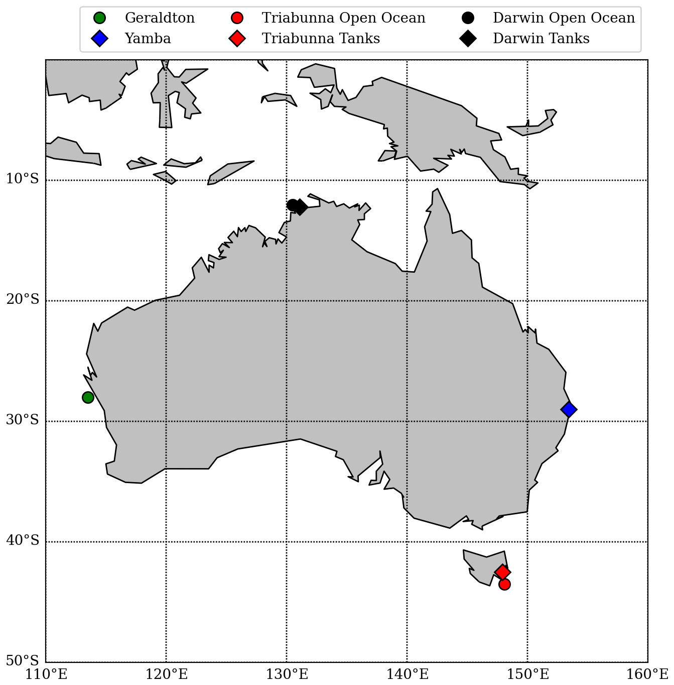
Figure 1 Locations of actual Asparagopsis farms in Geraldton, Triabunna, and Yamba and theoretical farms in Darwin.

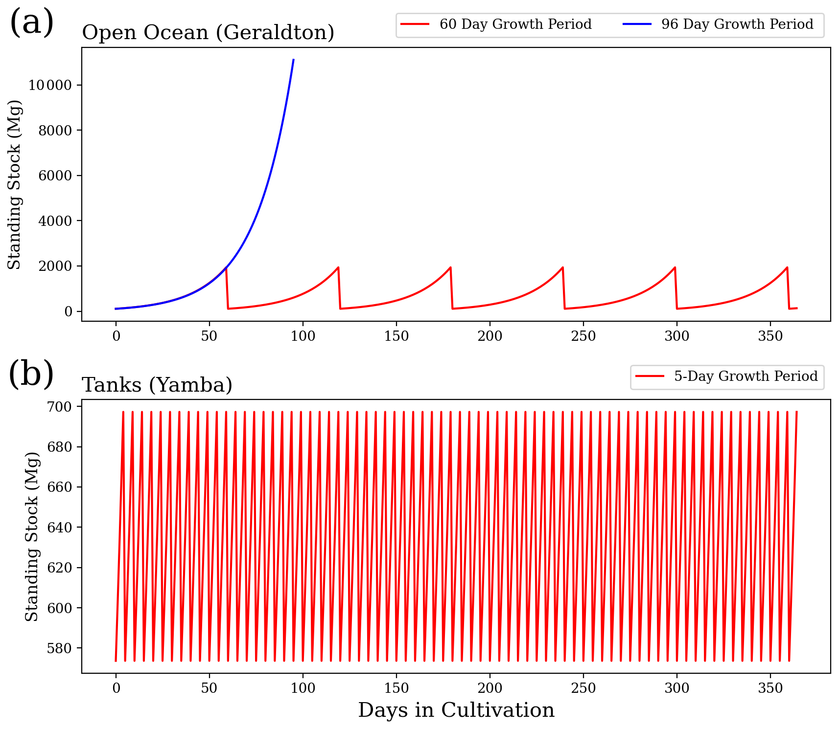
Figure 2 Standing stock biomass of Asparagopsis cultivation (a) in the open ocean for a 60 d growth period and 96 d growth period and (b) in terrestrial system culture for a 5 d growth period. Each of the three scenarios will achieve an annual yield of ∼1.6 × 10⁴ Mg DW.

2.2 Asparagopsis CHBr₃ release rates

Rates of the CHBr₃ content in Asparagopsis given in the literature range between 3.4 and 43 mg CHBr₃ g⁻¹ DW, with values around 10 mg CHBr₃ g⁻¹ DW appearing to be realistic in current cultivation (Burreson and Moore, 1976; Mata et al., 2012, 2017; Paul et al., 2006; Vucko et al., 2017). We assume that Asparagopsis strain selection cultivated for feed supplements will lead to high-yield CHBr₃ varieties; thus we assume augmented CHBr₃ production with a mean content of 21.7 mg CHBr₃ g⁻¹ DW (Magnusson et al., 2020) for this study.

Very few values on the CHBr₃ release from Asparagopsis have been reported in the literature. A constant release of 1100 ng CHBr₃ g⁻¹ DW h⁻¹ was measured for Asparagopsis armata tetrasporophyte, which has a CHBr₃ content of 14.5 mg CHBr₃ g⁻¹ DW (Paul et al., 2006). We assume a linear scaling between the CHBr₃ release rates and the content. Thus, a cultivated Asparagopsis for which we assume 21.7 mg CHBr₃ g⁻¹ DW should release around 1646 ng CHBr₃ g⁻¹ DW h⁻¹, a rate which has been confirmed by Marshall et al. (1999). Therefore, for our calculations, we assume a constant release of 1600 ng CHBr₃ g⁻¹ DW h⁻¹ for farmed Asparagopsis with a CHBr₃ content of 21.7 Mg CHBr₃ g⁻¹ DW. These content and release rates are higher than those for wild stock algae (Leedham et al., 2013; Nightingale et al., 1995) as the farming aims at algae varieties with high CHBr₃ yield. As available information on this topic is very sparse, no variations of the release rate with life-cycle stages, season, location, or other environmental parameters were used in this study. Also, the two species Asparagopsis armata and Asparagopsis taxiformis were treated the same way as Asparagopsis spp., as variations in CHBr₃ content and release within or between species are currently unknown (Mata et al., 2017), and more research on this topic is needed.

2.3 Parameterization of CHBr₃ emission

The emissions of CHBr₃ from farmed macroalgae are a function of the standing stock biomass (in grams of DW) and can be calculated with the constant release rate ($R_{{\mathrm{CHBr}}_{\mathrm{3}}})$ of 1600 ng CHBr₃ g⁻¹ DW h⁻¹ multiplied with the standing stock. The total release of CHBr₃ ($E_{{\mathrm{CHBr}}_{\mathrm{3}}})$ over the complete growth period of T days is given by the integral over the daily emissions from day 1 to day T:

$$\begin{array}{}\text{(2)}& \begin{array}{rl}{E}_{{\mathrm{CHBr}}_{\mathrm{3}}}=& \underset{\mathrm{0}}{\overset{T}{\int }}\mathrm{24}\cdot B_{\text{i}}\cdot (\mathrm{1}+\text{GR}{)}^t\cdot R_{{\mathrm{CHBr}}_{\mathrm{3}}}\mathrm{d}t\\ =& \mathrm{24}\cdot B_{\text{i}}\cdot R_{{\mathrm{CHBr}}_{\mathrm{3}}}\cdot {\displaystyle \frac{[{\left(\mathrm{1}+\text{GR}\right)}^T-\mathrm{1}]}{\ln (\mathrm{1}+\text{GR})}}\end{array}.\end{array}$$

For our atmospheric impact studies, we assume that all CHBr₃ released from the algae is emitted into the atmosphere at its location of production. An increasing seawater concentration of CHBr₃ shifts the equilibrium conditions between seawater and air towards the atmosphere, as CHBr₃ easily volatilizes to the atmosphere. Consequently, air–sea exchange acts as a relatively fast loss process for CHBr₃ in surface water. Oceanic sinks can also impact CHBr₃, but act on relatively long timescales. Degradation through halide substitution and hydrolysis results in the ocean sink CHBr₃ half-life of 4.37 years (Hense and Quack, 2009). Thus, most of the CHBr₃ contained in surface seawater is instantly outgassed into the atmosphere without oceanic loss processes, playing a role as confirmed by the modeling study of Maas et al. (2021).

The air–sea exchange of CHBr₃ is expressed as the product of its transfer coefficient (k_w) and the concentration gradient (Δc) (Eq. 3). The gradient is computed between the water concentration (c_w) and theoretical equilibrium water concentration (c_atm H⁻¹), where c_atm is the atmospheric concentration and H is Henry's law constant (Moore et al., 1995a, b).

$$\begin{array}{}\text{(3)}& F=k_{\text{w}}\cdot \mathrm{\Delta }c=k_{\text{w}}\cdot \left(c_{\text{w}}-{\displaystyle \frac{c_{\text{atm}}}{H}}\right)\end{array}$$

The compound-specific transfer coefficient (k_w) is determined using the air–sea gas exchange parameterization of Nightingale et al. (2000) (Eq. 4).

$$\begin{array}{}\text{(4)}& k_{\text{w}}=k\cdot \sqrt{Sc}/\mathrm{660}\end{array}$$

The transfer coefficient k is a function of the wind speed at 10 m height (u₁₀: $k=\mathrm{0.2}{u}_{\mathrm{10}}^{\mathrm{2}}+\mathrm{0.3}{u}_{\mathrm{10}}$), and the Schmidt number (Sc) is a function of sea surface temperature (SST) from Quack and Wallace (2003), which is expressed as $Sc=\mathrm{4662.8}-\mathrm{319.45}\cdot \text{SST}+\mathrm{9.9012}\cdot {\text{SST}}^{\mathrm{2}}+\mathrm{0.1159}\cdot {\text{SST}}^{\mathrm{3}}$.

In this study, we use the CHBr₃ sea-to-air flux climatology from Ziska et al. (2013) as marine background emissions. The global emission scenario from Ziska et al. (2013) is a bottom-up estimate of the oceanic CHBr₃ fluxes, generated from atmospheric and oceanic surface ship-borne in situ measurements between 1979 and 2013. Due to the paucity of data, the 35-year mean gridded data set was filled by interpolating and extrapolating the in situ measurement data. The oceanic emissions were calculated with the transfer coefficient parameterization of Nightingale et al. (2000) and 6-hourly meteorological data, which allow a temporal emission variability related to wind and temperature.

2.4 Emission scenarios for FLEXPART simulations

To quantify the atmospheric impact of CHBr₃ emissions from macroalgae farming, the Lagrangian particle dispersion model FLEXPART (Pisso et al., 2019) is used. FLEXPART has been evaluated extensively in previous studies (e.g., Stohl et al., 1998; Stohl and Trickl, 1999). The model includes moist convection and turbulence parameterizations in the atmospheric boundary layer and free troposphere (Forster et al., 2007; Stohl and Thomson, 1999). The European Centre for Medium-Range Weather Forecasts (ECMWF) reanalysis product ERA-Interim (Dee et al., 2011) with a horizontal resolution of ${\mathrm{1}}^{\circ }\times {\mathrm{1}}^{\circ }$ and 60 vertical model levels is used for the meteorological input fields, providing air temperature, winds, boundary layer height, specific humidity, and convective and large-scale precipitation with a 3 h temporal resolution.

We conduct FLEXPART simulations for the year 2018 with different emission scenarios as explained in the following and summarized in Table 1.

1. Australian scenarios. CHBr₃ emissions from the Asparagopsis farming in Geraldton, Triabunna, and Yamba are calculated for an overall annual yield of 34 674 Mg DW according to Eq. (2). For the terrestrial systems, 5 d growth periods are assumed, resulting in 73 harvests per year. For the open ocean, the assumption of different growth periods results in three sub-scenarios: (a) six 60 d growth periods with the first period starting on 1 January (referred to as GTY_O60), (b) one 96 d growth period starting on 1 January (GTY_O96_Jan), and (c) and another growth period starting on 1 July (GTY_O96_Jul).

   For the last Australian scenario, we assume that all farms are located around Darwin in the Northern Territory tropics with six 60 d growth periods in the open ocean and 73 5 d growth periods in the terrestrial systems (Darwin_O60). While this is an unlikely scenario according to current plans, it is useful to demonstrate the influence of potential farming locations on their environmental impact.

2. Global scenarios. Emissions from Asparagopsis farming in Geraldton, Triabunna, and Yamba are estimated according to the annual yield, upscaled by a factor of 30 to global requirements, amounting to 1.04 × 10⁶ Mg DW. Growth periods and harvesting frequencies are set up in the same way as for the Australian scenarios. Short names of the global scenarios are the same as for the Australian scenarios with the additional label 30x.

3. Background scenario. Emissions from Ziska et al. (2013) for the entire coastal region around Australia defined as all ${\mathrm{1}}^{\circ }\times {\mathrm{1}}^{\circ }$ grid cells directly neighboring the coastline (Ziska_Coast).

4. Extreme event scenarios.  We assume extreme conditions where a hypothetical tropical cyclone causes implausible release of all CHBr₃ from the macroalgae farm and water into the atmosphere. We focus on the case study of Geraldton and the tropical cyclone Joyce, which occurred from 6–13 January 2018 around western Australia. We base the amount of available macroalgae biomass on the Australian scenario and assume that the entire CHBr₃ content of all Asparagopsis at this location is released at once. The two scenarios defined here assume that the tropical cyclone occurs at the end of the 60 d growth period (Geraldton_Ex60), resulting in the release of 41.8 Mg CHBr₃ (21.7 mg CHBr₃ g⁻¹ DW ⋅ 1926 Mg DW), or at the end of the 96 d growth period (Geraldton_Ex96), resulting in the release of 250.8 Mg CHBr₃ (21.7 mg CHBr₃ g⁻¹ DW ⋅ 11 558 Mg DW).

   The daily model output is recorded for all simulations. For the extreme event, which assumes the destruction of a farm (Geraldton-Ex), the 3-hourly output is recorded. For all simulations, except the background scenario and extreme scenario, trajectories are released from four regions with the following size: (a) Geraldton (open ocean, 11 558 ha), ${\mathrm{0.1}}^{\circ }\times {\mathrm{0.1}}^{\circ }$; (b) Triabunna (open ocean, 4623 ha), ${\mathrm{0.06}}^{\circ }\times {\mathrm{0.06}}^{\circ }$; (c) Triabunna (terrestrial systems, 126 ha), ${\mathrm{0.01}}^{\circ }\times {\mathrm{0.01}}^{\circ }$; and (d) Yamba (terrestrial systems, 210 ha), ${\mathrm{0.01}}^{\circ }\times {\mathrm{0.01}}^{\circ }$. For the tropical and extreme scenarios, trajectories are released from the Darwin and Geraldton farms, respectively. For the background scenario Ziska_Coast, trajectories are released from the ${\mathrm{1.0}}^{\circ }\times {\mathrm{1.0}}^{\circ }$ grid along the Australian coastline. Note that it is not reasonable to compute the Ziska emission on the locations of farming as some farms are terrestrial. However, if we assume all the farms are Geraldton-like (i.e., all grown in the open ocean), the Ziska emission in Geraldton, Yamba, and Triabunna will be 843, 295, and 676 Mg, respectively. The amount of released CHBr₃ is evenly distributed among the trajectories and is depleted during the Lagrangian simulations according to the atmospheric half-life of 17 d (e-folding lifetime of 24 d) (Hossaini et al., 2010; Montzka and Reimann et al., 2010; Engel et al., 2018).

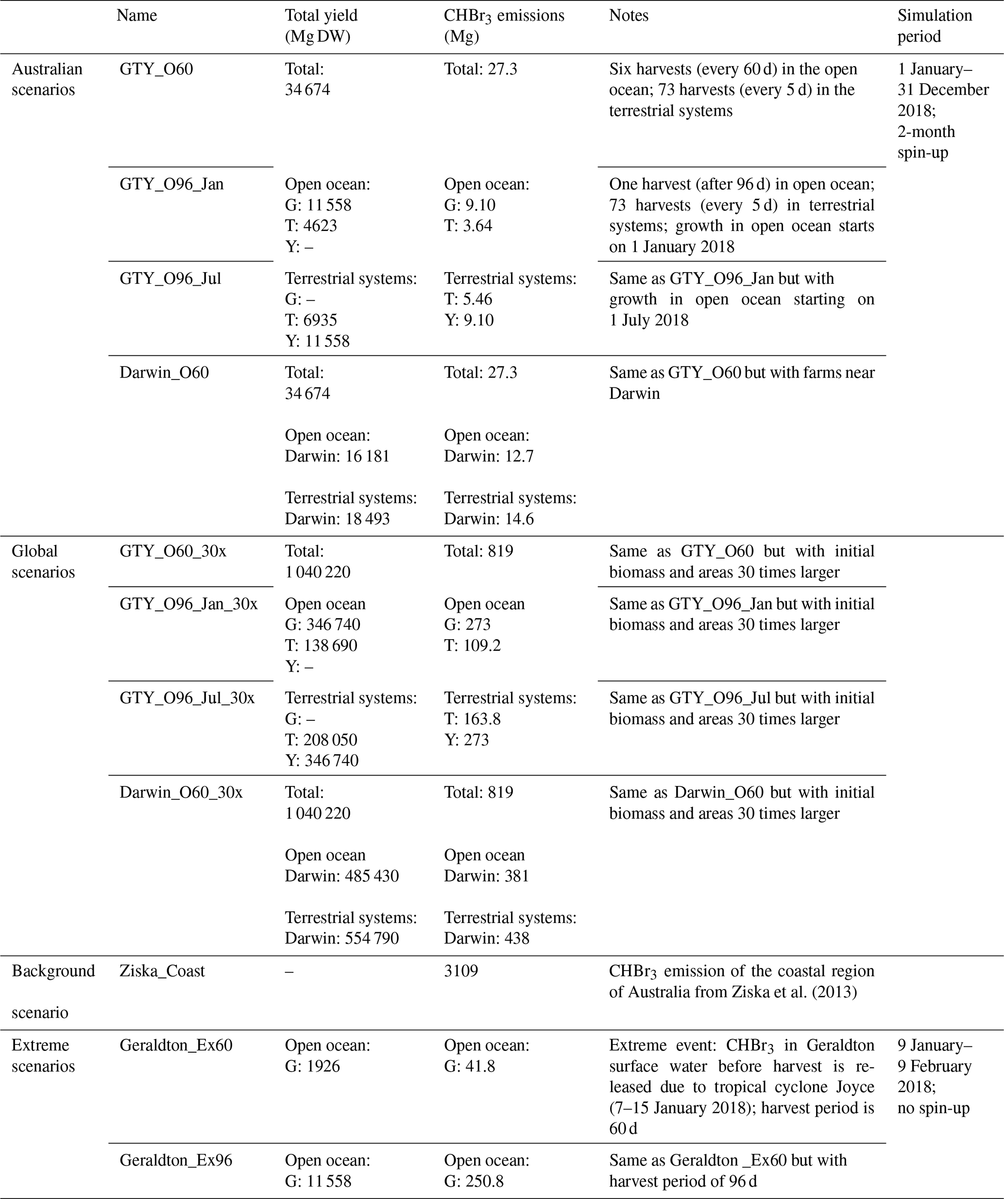
Table 1 Detailed information on the scenarios set up for the atmospheric transport simulations with FLEXPART (Geraldton, Triabunna, and Yamba: GTY).

2.5 Ozone depletion potential (ODP)

The ozone depletion potential (ODP) is defined as the time-integrated potential destructive effect of a substance to the ozone layer relative to that of the reference substance CFC-11 (CCl₃F) on a mass-emitted basis (Wuebbles, 1983). The ODP is a well-established and extensively used concept traditionally defined for anthropogenic long-lived halocarbons. However, the concept has been also applied to VSLSs (Brioude et al., 2010; Pisso et al., 2010): unlike the ODP for long-lived halocarbons, which is one constant number, the ODP of a VSLS is a function of time and location of the emissions. This variable number still describes the time-integrated ozone depletion resulting from a CHBr₃ unit mass emission relative to the ozone depletion resulting from the same unit mass emission of CFC-11. The ODP for VSLSs can be derived from chemistry–climate or chemistry transport models simulating the changes of ozone due to certain compounds (Claxton et al., 2019; Zhang et al., 2020). The trajectory-derived ODP of VSLSs such as CHBr₃ is calculated as a function of location and time of the potential emissions (Brioude et al., 2010; Pisso et al., 2010). As for the traditional ODP concept, the time- and space-dependent ODP describes only the potential of a compound but not its actual damaging effect to the ozone layer and is independent of the total emissions. It is noteworthy that many VSLSs including CHBr₃ can impact ozone in the troposphere and stratosphere. As ODPs are used to assess stratospheric ozone depletion only, the contribution of VSLSs to tropospheric ozone destruction needs to be excluded when calculating their ODP (Pisso et al., 2010; Zhang et al., 2020). The trajectory-based ODP from Pisso et al. (2010) used in this study considers only the impact of CHBr₃ on the stratospheric ozone instead of the ozone column. The fraction of originally emitted VSLSs reaching the stratosphere depends strongly on the meteorological conditions. In particular, it shows a pronounced seasonality. Here we apply ODP values adapted from Pisso et al. (2010), originally calculated for a VSLS with a lifetime of 20 d, which is very similar to that of CHBr₃. ODPs for VSLSs are calculated by means of combining two sources of information: one corresponding to the slow stratospheric branch and the other to the fast tropospheric branch of transport. The former is uniform for all species modeled and is based on the calculation of the expected stratospheric residence time of a Lagrangian particle entering the stratosphere. The latter is based on the probability of stratospheric injection of a given unit emission of the tracer at the ground. The probability of injection depends not only on the fraction of air reaching the tropopause but also on the time the air mass takes from the ground to the tropopause. This is because during the transit of the air mass through the troposphere, the precursor is chemically degraded, and the solubility of the products leads to mass loss due to wet deposition.

In this study, we present the ODP-weighted emissions, which combine the information of the ODP and surface emissions and are calculated by multiplying the CHBr₃ emissions with the trajectory-derived ODP at each grid point. The ODP-weighted emissions provide insight into key factors of CHBr₃ emission (i.e., where and when CHBr₃ is emitted) that impact stratospheric ozone (Tegtmeier et al., 2015). The absolute values are subject to relatively large uncertainties arising from uncertainties in the parameterization of the convective transport. Furthermore, the ODP values applied here do not consider product gas entrainment and therefore provide a lower limit of the impact of CHBr₃ on stratospheric ozone. Taking into account product gas entrainment can lead to 30 % higher ODP values (Engel et al., 2018; Tegtmeier et al., 2020) but has no large impact on the comparison between global ODP-weighted CHBr₃ emissions and farm-based ODP-weighted CHBr₃ emissions presented here.

3 CHBr₃ emission and atmospheric mixing ratio

3.1 CHBr₃ emissions

As shown in Eq. (2), the total CHBr₃ emissions are determined by the growth rate, growth period, and initial biomass. For our scenarios based on selected fixed growth rates, the growth periods are adjusted so that the intended annual yield (∼3.5 × 10⁴ Mg DW) is achieved. We conduct a sensitivity study to analyze how much the total emissions change for variations in the length and number of the growth periods for a fixed annual yield. For this purpose, we compare Geraldton farming for GTY_O60 (open ocean, six 60 d growth periods) with Geraldton farming for GTY_O96 (open ocean, one 96 d growth period) and Yamba farming for GTY_O60 (terrestrial systems, 73 growth periods of 5 d). Our estimates show that the annual release of CHBr₃ from Asparagopsis is the same for all three case studies (Fig. 3a), confirming that for a fixed annual yield and growth rate, the culture conditions of open-ocean and tank farming are not important for VSLS emissions.

A second sensitivity study investigates the variations in CHBr₃ emissions for different growth rates and the same fixed annual yield. For this purpose, we compare Geraldton farming (open ocean, with an intended annual yield of ∼1.1 × 10⁴ Mg DW) for different growth rates varying between 1 % and 10 %. The scenario with a 5 % growth rate corresponds to Geraldton farming for GTY_O60 (open ocean, six 60 d growth periods), while for the other growth rates the growth periods have been adjusted to achieve the same annual yield.

The CHBr₃ emissions depend strongly on the growth rates (Fig. 3b), with emission calculated for a 1 % growth rate being almost 10 times higher than the emissions calculated for a 10 % growth rate. For a lower growth rate, the initial biomass needs to be higher to achieve the targeted seaweed yield (∼1.1 × 10⁴ Mg) after 1 year and/or the growth period needs to be longer, thus resulting in larger amounts of biomass in the ocean and higher annual CHBr₃ emissions. Vice versa, for higher growth rates, the annual oceanic biomass is smaller and total emissions are lower.

The overall emissions from the intended Australian seaweed farming of ∼3.5 × 10⁴ Mg DW range from 13.5 Mg (0.05 Mmol) for a 10 % growth rate to 134 Mg (0.5 Mmol) per year for a 1 % growth rate. For the growth rates higher than 5 %, the differences of CHBr₃ emissions are less significant than those derived for the lower growth rates. In our study, we choose 5 % growth rate as representative, which leads to emissions of ∼27 Mg (0.1 Mmol) CHBr₃ per year for the targeted final yield. For the global scenario with an annual yield of ∼1.0 × 10⁶ Mg DW (30 times the Australian target), the emissions would range from 412 Mg (1.6 Mmol) to 4014 Mg (16 Mmol) per year, with the annual emission of 810 Mg (3.2 Mmol) for 5 % growth rates.

Interestingly, the potential local emissions for all the farming scenarios are generally 3 to 6 orders of magnitude higher than the background coastal emissions. The maximum climatological emissions derived from available observations (Ziska_Coast) are around 2000 pmol m⁻² h⁻¹ for the coastal waters of Australia, while the emissions from an Asparagopsis farm can reach more than 2.0 × 10⁶ pmol (2 µmol) m⁻² h⁻¹ from a terrestrial system and more than 5.0 × 10⁵ pmol m⁻² h⁻¹ from the open ocean. These differences are to a large degree related to the fact that the Ziska_Coast is given on a ${\mathrm{1.0}}^{\circ }\times {\mathrm{1.0}}^{\circ }$ grid, with high coastal values averaging out over the relatively wide grid cells, while the values derived for the farms applying to much smaller areas. Tank emission rates (${\mathrm{0.01}}^{\circ }\times {\mathrm{0.01}}^{\circ }$) and open-ocean farming emission rates (${\mathrm{0.1}}^{\circ }\times {\mathrm{0.1}}^{\circ }$) averaged over a ${\mathrm{1}}^{\circ }\times {\mathrm{1}}^{\circ }$ grid cell result in 200 pmol CHBr₃ m⁻² h⁻¹ and 5000 pmol CHBr₃ m⁻² h⁻¹, respectively, thus being very similar to the Ziska emissions.

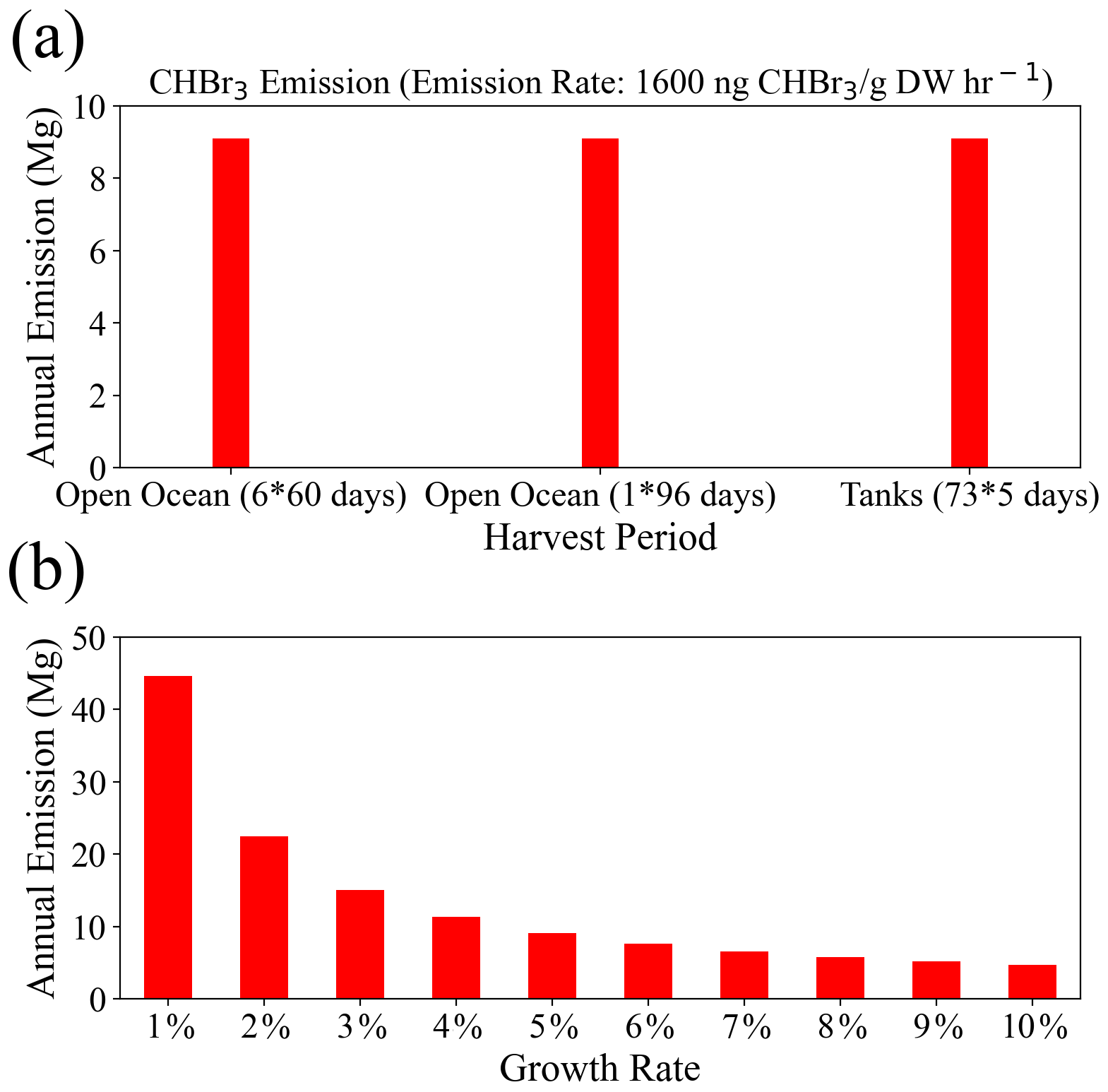
Figure 3 The annual release of CHBr₃ (Mg yr⁻¹) from (a) the same growth rate (5 %) for different growth periods and (b) under different growth rates but with the same initial biomass. Both (a) and (b) are obtained with a total annual yield of 11 558 Mg DW.

3.2 Atmospheric CHBr₃ mixing ratio

We use the CHBr₃ emissions calculated in Sect. 3.1 to simulate the enhanced atmospheric CHBr₃ mixing ratios (above natural background) for each Asparagopsis farming scenario. Background CHBr₃ levels are calculated based on the Ziska et al. (2013) Australian coastal emissions (Ziska_Coast). The temporal evolution of CHBr₃ mixing ratio with height shows that the CHBr₃ resulting from the Australian farming scenarios are negligible (see Fig. S1 in the Supplement) compared to the coastal background emissions of Australia (Ziska_Coast).

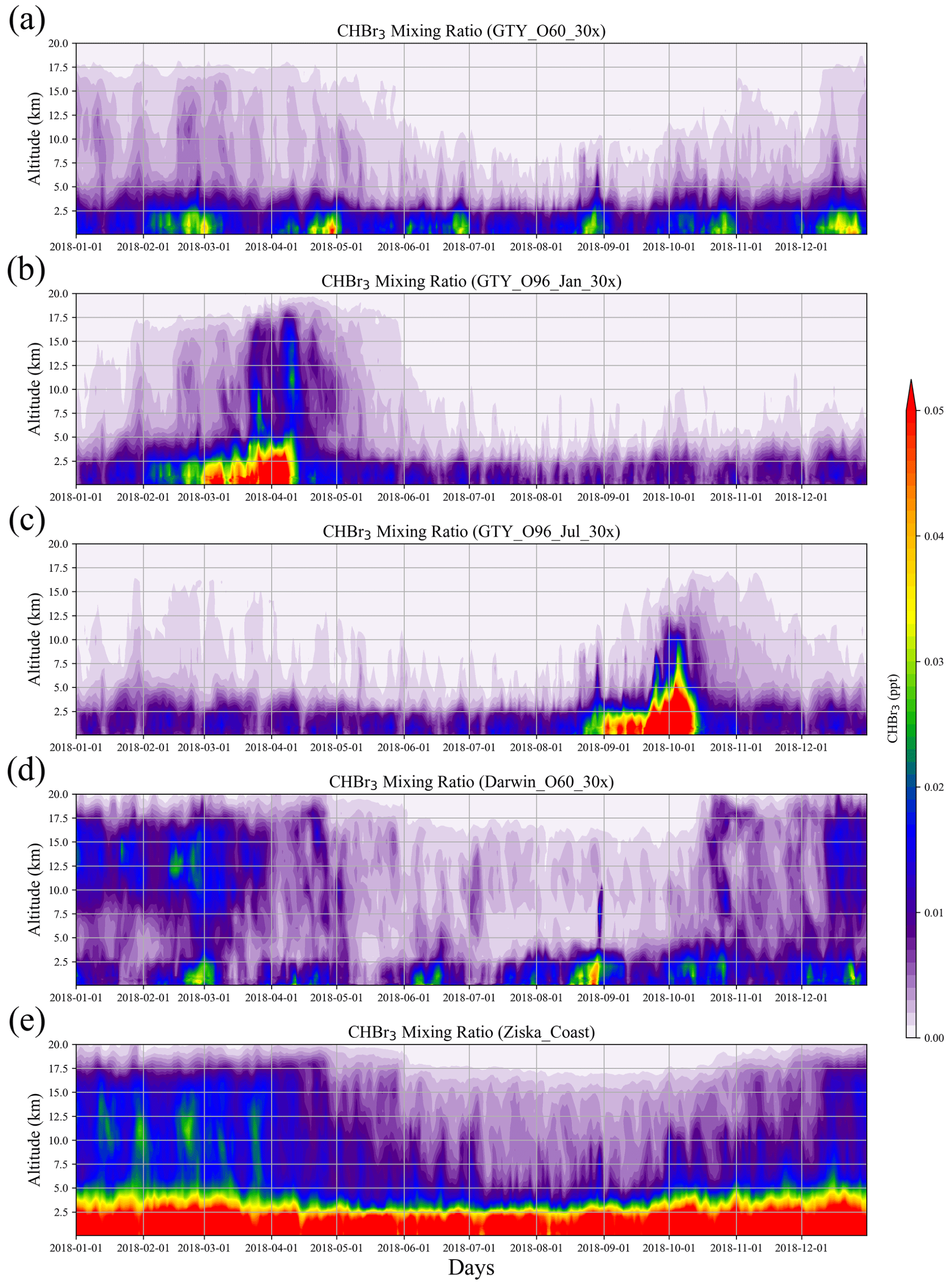
Figure 4 Altitude–time cross sections of CHBr₃ mixing ratio averaged over 10–45^∘ S, 105–165^∘ E from global scenarios (a) GTY_O60_30x, (b) GTY_O96_Jan_30x, (c) GTY_O96_Jul_30x, and (d) Darwin_O60_30x and background scenario (e) Ziska_Coast.

For the global scenarios (Fig. 4), atmospheric CHBr₃ is comparable to CHBr₃ resulting from Australian coastal background emissions, especially near the end of the growth period in the open ocean. For almost all scenarios (except for GTY_O96_Jul_30x), the emissions generally reach higher into the atmosphere in the first 3 months of the year with enhanced values around 15 km, reflecting the stronger convection during austral summer. For open-ocean emissions occurring during late austral winter (GTY_O96_Jul_30x, Fig. 4c), high CHBr₃ mixing ratios are found around September, however at a lower altitude range compared to the equivalent scenario with open-ocean emission occurring during late austral summer (GTY_O96_Jan_30x; Fig. 3b).

The spatial distribution of annual mean CHBr₃ at 1 km (Fig. 5) further confirms the insignificance of the signals from the Australian farming scenarios compared with the background CHBr₃ values. For the global scenarios, localized regions of high mixing ratios are found near the locations of the farms due to the stronger emission. For Darwin_O60_30x, the belt of high mixing ratios is extended northwestward, due to the prevailing easterlies in the tropics. At higher altitudes (e.g., 5 and 15 km; Figs. S2–S3), localized high CHBr₃ is only found near Darwin for the Darwin_O60_30x scenario, reflecting that strong tropical convection is needed to transport short-lived gases to such altitudes.

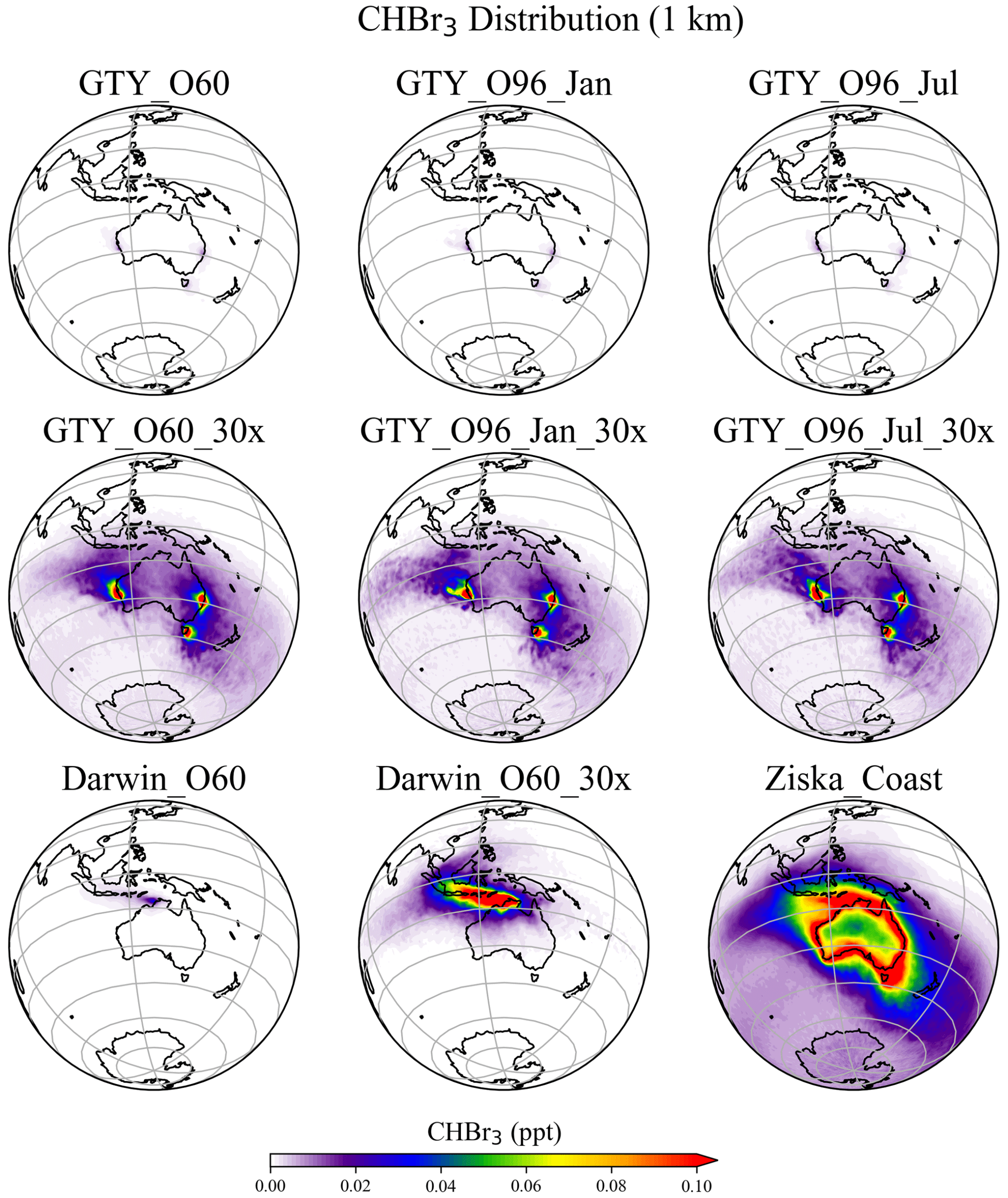
Figure 5 Annual mean CHBr₃ spatial distribution from GTY_O60, GTY_O60_30x, GTY_O96_Jan, GTY_O96_Jan_30x, GTY_O96_Jul, GTY_ O96_Jul_30x, Darwin_O60, Darwin_O60_30x, and Ziska_Coast at 1 km altitude.

The results above suggest that in the boundary layer, global scenarios and extreme events could lead to CHBr₃ mixing ratios comparable to those from the background scenario. Only in the global tropical scenario (Darwin_O60_30x) can CHBr₃ mixing ratios, which are larger than the background values, be found at high altitudes (Fig. 4).

Simulations of the two extreme scenarios (Geraldton_Ex) for 60 and 96 d growth periods are shown in Fig. 6. For the Geraldton_Ex simulations, we assume the implausible scenario that the farm could be totally damaged by cyclone Joyce on the day of harvest in January, and the total CHBr₃ content of the Asparagopsis stock was simultaneously released to the atmosphere during the event. Both scenarios lead to significant CHBr₃ mixing ratios in the atmosphere, especially at altitudes below 5 km. Among the two scenarios, the Geraldton_Ex96 contributes the larger amount of CHBr₃ emission, as the macroalgae experienced a longer growth period, so the biomass was higher and had accumulated more CHBr₃. When averaged over the same period (9–26 January 2018), the CHBr₃ mixing ratios from Geraldton_Ex96 are much larger than those from Ziska_Coast (Fig. 6) below 5 km, and signals with comparable magnitudes, though with smaller coverage, are found at 15 km.

As mentioned in Sect. 3.1, the local CHBr₃ emissions due to the seaweed cultivation are generally higher than coastal emission given on a 1.0^∘ × 1.0^∘ grid. However, due to the relatively small spatial extent of the farms, the emissions quickly dilute in the atmosphere, and the magnitude of the mixing ratios declines rapidly off the coast and vertically.

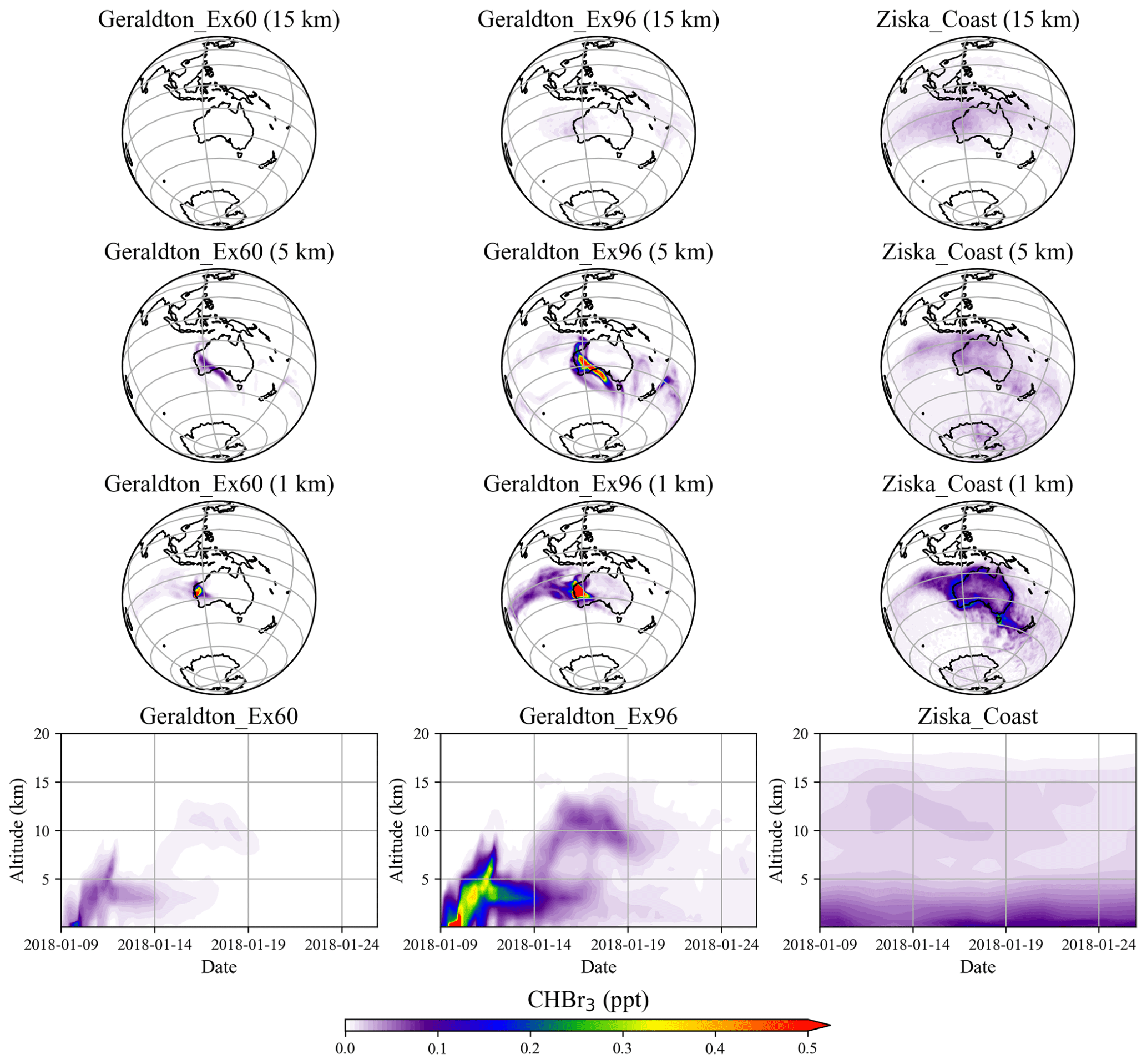
Figure 6 The 17 d average of spatial distribution and altitude–time cross sections of CHBr₃ mixing ratio averaged over 10–45^∘ S, 105–165^∘ E for Geraldton_Ex60, Geraldton_Ex96, and Ziska_Coast.

4 Ozone depletion potential for CHBr₃

The ODP distribution from Pisso et al. (2010) for the region around Australia, Southeast Asia, and the Indian Ocean for the Southern Hemisphere (SH) summer and winter is shown in Fig. 7. The ODP distribution changes strongly with season as the transport of short-lived halogenated substances such as CHBr₃ depends on the seasonal variations in the location of the Intertropical Convergence Zone (ITCZ). The highest ODP values of 0.5, which imply that any amount (per mass) of CHBr₃ released from the specific location will destroy half as much stratospheric ozone as the same amount of CFC-11 released from this location, are found during July over the maritime continent and during January over the west Pacific south of the Equator. The northern Australian coastline shows the highest ODP values during January when the thermal Equator and the ITCZ are shifted southwards and ODP values for Yamba and Darwin are 0.26 and 0.29, respectively. The other two locations as well as all four locations during SH winter show ODP values of only up to 0.1.

As demonstrated in Sect. 3, the total annual CHBr₃ emissions from any location are independent of the details of the farming practice; however, the ODP-weighted emissions change for the different scenarios as the growth periods fall into different seasons with varying ODP values. In general, the scenario of one harvest period in SH summer leads to larger ODP-weighted emissions when compared to the same biomass harvested throughout the year. In addition to the harvesting practice, the locations of the farms have a large impact on the efficiency of the CHBr₃ transport to the stratosphere and thus on the ODP-weighted emissions.

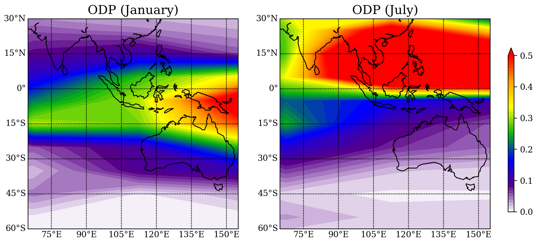
Figure 7 Spatial distribution of the ODP in January and July from Pisso et al. (2010), plotted with interval of 0.01.

The ODP-weighted emissions of CHBr₃ for different emission scenarios are shown in Fig. 8. Asparagopsis farming at GTY (GTY_O60) leads to additional CHBr₃ emissions of up to 2.53 Mg yr⁻¹. If all farming (∼3.5 × 10⁴ Mg DW Asparagopsis) occurs in Darwin (Darwin_O60), ODP-weighted emissions would increase to 6.48 Mg CHBr₃ yr⁻¹. In comparison, all naturally occurring emissions around the Australian coastline (Ziska_coast) lead to ODP-weighted CHBr₃ emissions of 221.52 Mg yr⁻¹. In consequence, Asparagopsis farming in the three locations Geraldton, Triabunna, and Yamba would lead to an increase in the ODP-weighted emissions from Australian coastal emissions of 1.14 %. If all farming would take place in Darwin, ODP-weighted CHBr₃ emissions would increase by 2.93 %.

As the global ODP-weighted emissions were estimated to be around 4.0 × 10⁴ Mg yr⁻¹ (bottom-most bar in Fig. 8, Tegtmeier et al., 2015), the additional contribution due to the Australian farming scenarios in GTY or Darwin would be negligible, increasing the contribution of CHBr₃ emissions to ozone depletion by 0.006 % and 0.016 %, respectively. Even if the farming were upscaled to cover the global needs (∼1.0 × 10⁶ Mg DW), the ODP-weighted CHBr₃ emissions would only increase to 75 and 195 Mg for farming in GTY (GTY_O60_30x) and Darwin (Darwin_O60_30x), respectively. Thus produced CHBr₃ would increase the current contribution of CHBr₃ to stratospheric ozone depletion by 0.19 % and 0.48 %, which is again a very small contribution.

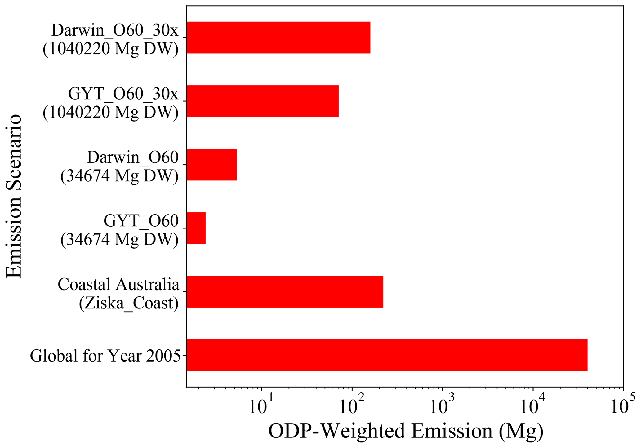
Figure 8 The ODP-weighted emissions of CHBr₃ for global scenarios (GTY_O60_30x and Darwin_O60_30x), Australian scenarios (GTY_O60 and Darwin_O60), coastal Australian emission (Ziska_Coast), and global ODP-weighted emission for 2005 taken from Tegtmeier et al. (2015) as a reference; note that the x axis is exponential.

To assess the increase in the ODP-weighted CHBr₃ emissions under the most extreme and implausible conditions, we envision the total harvest of 1 year, which contains 752 Mg (21.7 mg CHBr₃ g⁻¹ DW ⋅ 34 674 Mg DW) CHBr₃, stored in a warehouse of 50 m × 25 m × 5 m in either of the four locations. We assume that the facility is destroyed, and all 750 Mg is released to the atmosphere. Then maximum ODP-weighted CHBr₃ emissions would occur for the release in Darwin during January and amount to 215.9 Mg, almost doubling the ODP-weighted coastal CHBr₃ emissions of Australia. If the entire content of ∼1.0 × 10⁶ Mg Asparagopsis DW (21.7 mg CHBr₃ g⁻¹ DW ⋅ 1 040 220 Mg DW = 22 573 Mg CHBr₃) were released in Darwin, the additional contribution of CHBr₃ to global ozone depletion could reach 16 %.

5 Summary and conclusions

In this study, we assessed the potential risks of CHBr₃ released from Asparagopsis farming near Australia for the stratospheric ozone layer by analyzing different cultivation scenarios. We conclude that the intended operation of Asparagopsis seaweed cultivation farms with an annual yield of 34 674 Mg DW in either open-ocean or terrestrial cultures at the locations Triabunna, Yamba, Geraldton, and Darwin will not impact the ozone layer under normal operating conditions.

For Australia scenarios with an annual yield of ∼3.5 × 10⁴ Mg DW and algae growth rate of 5 % d⁻¹, the expected annual CHBr₃ emission from the considered Asparagopsis farms into the atmosphere (∼27 Mg, 0.11 Mmol) is less than 0.9 % of the coastal Australian emissions (∼3109 Mg, 12.3 Mmol). This contribution is negligible from a global perspective by adding less than 0.01 % to the worldwide CHBr₃ emissions from natural and anthropogenic sources. The overall emissions from the farms would be even smaller with a faster growth rate for the same annual yield. We have assumed a high CHBr₃ production of 21.7 mg g⁻¹ DW from superior strains and expected lower CHBr₃ production of 14 mg g⁻¹ DW would likewise reduce emissions to the atmosphere.

The CHBr₃ emissions from the localized Asparagopsis farms could be larger than emissions from coastal Australia. However, the overall atmospheric impact of the Asparagopsis farms is negligible, as the CHBr₃ dilutes rapidly and degrades in the atmosphere under normal weather conditions. Mixing ratios of CHBr₃ are generally dominated by the coastal Australian emissions. In global scenarios with annual yield ∼1.0 × 10⁶ Mg DW, localized CHBr₃ mixing ratios comparable to the background values can be found in the lower troposphere. In the upper troposphere, on the other hand, mixing ratios larger than background values only appear in the global tropical scenario (Darwin_O60_30x). The release of the complete CHBr₃ content from the macroalgae to the environment on very short timescales (e.g., days) due to extreme weather situations could contribute significant amounts to the atmosphere, especially during times when the standing stock biomass is relatively large (Geraldton_Ex96). While such extreme scenarios could lead to much larger mixing ratios than background values, such mass release events are implausible because even if a farm were totally destroyed the seaweed stock could not instantaneously release all the accumulated CHBr₃. Such scenarios have been included here to evaluate a catastrophic and likely impossible worst-case scenario.

The impact of CHBr₃ from the proposed seaweed farms on the stratospheric ozone layer is assessed by weighting the emissions with the ozone depletion potential of CHBr₃. In total, Australia scenarios could lead to additional ODP-weighted CHBr₃ emissions of up to 2.53 Mg yr⁻¹ with farms located in Geraldton, Triabunna, and Yamba. With all farming performed in Darwin (Darwin_O60), the emitted CHBr₃ could reach the stratosphere on shorter timescales, and ODP-weighted emissions would increase to 6.48 Mg, which is less than 0.02 % of the global ODP-weighted emissions. For the global tropical scenario (Darwin_O60_30x), the ODP-weighted emissions amount to 175 Mg, increasing the global ozone depletion by 0.48 %, resulting in a very small contribution. The ODP used in this study does not include the impact of VSLS product gases. Previous modeling studies have highlighted the role of product gas treatment and their impact on the stratospheric halogen budget (e.g., Fernandez et al., 2021). Including product gas entrainment can lead to up to 30 % larger ODP values for CHBr₃ (Engel et al., 2018; Tegtmeier et al., 2020); thus the ODP-weighted emissions presented here can be up to 30 % larger. However, this does not affect our assessment of the potential importance of cultivation-induced CHBr₃ as the ratios of the impact of each scenario compared with the global ODP-weighted emissions remain the same. New CHBr₃ measurements in Cape Grim close to Triabunna show larger CHBr₃ mixing ratios (∼1.5 ppt, Dunse et al., 2020) than the Ziska climatology (∼0.8 ppt, Ziska et al., 2013). Similarly, the Ziska climatology is known to underestimate water concentrations of CHBr₃ in coastal regions with spare local measurements (Ziska et al., 2013; Maas et al., 2021). While the new atmospheric measurements suggest that a higher flux is required than currently included in the Ziska climatology, updated air–sea flux values can only be derived for simultaneous measurements in water and air, which are currently not available. It is important to note that such updated air–sea flux estimates would only impact the conclusions of our study if they were much lower than the old estimates over large parts of the Australian coastline, a scenario which is highly unlikely.

We note that all data characterizing the potential systems for the production of Asparagopsis are based on few available literature data, laboratory-scale tests, and relatively small-scale field trials. This not only places limitations on the technological representativeness of a future system and the temporal validity of the study, but also demonstrates importance for directed studies, especially on the release of CHBr₃ from Asparagopsis during cultivation. As this understanding evolves so will the cultivation and processing technologies engineered to conserve the antimethanogenic CHBr₃ in the seaweed biomass, which is the primary value feature of Asparagopsis. These limitations are largely mitigated in our study by evaluating various environmental and meteorological conditions ranging from conservative to the most extreme scenarios and by investigating different farming practices based on various sensitivity studies.