Evaluation of modelled summertime convective storms using polarimetric radar observations

Ensemble simulations with the Terrestrial Systems Modelling Platform (TSMP) covering northwestern Germany are evaluated for three summertime convective storms using polarimetric X-band radar measurements. Using a forward operator, the simulated microphysical processes have been evaluated in radar observation space. Observed differential reflectivity (Z_DR) columns, which are proxies for updrafts, and multi-variate fingerprints for size sorting and aggregation processes are captured by the model, but co-located specific differential phase (K_DP) columns in observations are not reproduced in the simulations. Also, the simulated Z_DR columns, generated by only small-sized supercooled drops, show smaller absolute Z_DR values and a reduced width compared to their observational counterparts, which points to deficiencies in the cloud microphysics scheme as well as the forward operator, which does not have explicit information of water content of ice hydrometeors. Above the melting layer, the simulated polarimetric variables also show weak variability, which can be at least partly explained by the reduced particle diversity in the model and the inability of the T-matrix method to reproduce the polarimetric signatures of snow and graupel; i.e. current forward operators need to be further developed to fully exploit radar data for model evaluation and improvement. Below the melting level, the model captures the observed increase in reflectivity, Z_DR and specific differential phase (K_DP) towards the ground.

The contoured frequency altitude diagrams (CFADs) of the synthetic and observed polarimetric variables were also used to evaluate the model microphysical processes statistically. In general, CFADs of the cross-correlation coefficient (ρ_hv) were poorly simulated. CFADs of Z_DR and K_DP were similar but the model exhibits a relatively narrow distribution above the melting layer for both, and a bimodal distribution for Z_DR below the melting layer, indicating either differences in the mechanism of precipitation formation or errors in forward operator which uses a functional form of drop size distribution.

In general, the model was found to underestimate the convective area fraction, high reflectivities, and the width/magnitude of Z_DR columns, all leading to an underestimation of the frequency distribution for high precipitation values.

1 Introduction

The representation of cloud and precipitation processes in atmospheric models is a central challenge for numerical weather prediction and climate projections (e.g. Boucher et al., 2013; Bauer et al., 2015). Especially, the parameterization of cloud microphysical processes and its interaction with the resolved dynamics need to be well tuned in order to provide dependable predictions (Igel et al., 2015; Brown et al., 2016; Morrison et al., 2020). In numerical models, the cloud microphysics is parameterized either using the so-called spectral (bin) approach or single/multi-moment bulk formulations, with the latter most common in numerical weather prediction (NWP) models due to computational efficiency (Khain et al., 2000). These parameterizations are often constrained using in situ and/or radar reflectivity observations. While in situ measurements by aircraft are sparse, ground-based radar observations provide three-dimensional structure of microphysical processes and are thus increasingly used for in-depth numerical modelling evaluation (e.g. Noppel et al., 2010; Min et al., 2015; Tao et al., 2016, of many others). Besides horizontal reflectivity Z_H, polarimetric radar observations provide estimates of differential reflectivity Z_DR, specific differential phase K_DP, and cross-correlation coefficient ρ_hv, which depend on hydrometeor shape, orientation, density and phase composition, and thus enable a more detailed evaluation of the modelled microphysical and macrophysical processes (Andrić et al., 2013; Snyder et al., 2017a; Putnam et al., 2017). However, this research field is still relatively new, partly because polarimetric precipitation radar networks became just recently available. The upgrade of the United States National Weather Service (NWS) S-band weather surveillance radar 1988 Doppler (WSR-88D) network to polarimetry was completed in 2013, while Germany completed the upgrade of its national C-band network in 2015 in parallel with other European countries.

Measured polarimetric variables are the result of the average scattering characteristics of the ensemble of hydrometeors contained in a resolved radar resolution volume and are expressed as second-order moments or correlations and powers of the horizontally and vertically polarized signals (Ryzhkov and Zrnic, 2019). Polarimetric variables are affected by hydrometeor shape/size distribution, concentration, orientation and phase composition, but all to a different extent and therefore the multivariate fingerprints provides insights into various microphysical processes like size sorting, evaporation, aggregation, riming, melting, secondary ice production, hail production, etc. Horizontal reflectivity (Z_H) especially provides information on the size and with that on ongoing aggregation/riming processes. Differential reflectivity (Z_DR) mainly provides information on the shape of hydrometeors and does not depend on the number concentration, while specific differential phase (K_DP) is proportional to the concentration of hydrometeors, thereby providing insight into the generation of new snow in the dendritic growth layer (Trömel et al., 2019). Cross-correlation coefficient (ρ_hv) is mainly a measure of the hydrometeor diversity in the resolved radar resolution bin. This information can be used for numerical model evaluation using two approaches: (1) the comparison of simulated mixing ratios or process rates with microphysical and thermodynamic retrievals from radar observations and (2) the direct comparison in radar observation space exploiting synthetic measurements obtained from a forward operator (Ryzhkov et al., 2020; Trömel et al., 2021). While both approaches have uncertainties caused by inherent assumptions, the latter method recently received more attention in the community due to increasingly available forward operators (e.g. Pfeifer et al., 2008; Xie et al., 2016; Heinze et al., 2017; Wolfensberger and Berne, 2018; Kumjian et al., 2019; Matsui et al., 2019; Oue et al., 2020), but requires awareness of assumptions made in both the model and the forward operator (FO). Even though first polarimetric forward operators have been already available several years ago, like SynPolRad introduced in Pfeifer et al. (2008), refinements are still ongoing and mandatory for a full exploitation. For example, Shrestha et al. (2022) and Trömel et al. (2021) demonstrated the limitations of the T-matrix method and its assumption of oblate spheroids used in current forward operators to reproduce the polarimetric signatures of low-density particles like dry snow aggregates and motivated further research towards a full exploitation of radar observations for model evaluation. The connection to a scattering data base would be key for a better representation of the ice phase. Furthermore, several other key tools became just recently available or are still under development (Trömel et al., 2021). Besides, many previous studies have documented polarimetric signatures of deep convective storms in S-band or C-band observations (e.g. Kumjian and Ryzhkov, 2008; Jung et al., 2010, 2012; Kumjian and Ryzhkov, 2012; Homeyer and Kumjian, 2015; Kaltenboeck and Ryzhkov, 2013; Johnson et al., 2016; Ilotoviz et al., 2018), while studies based on higher-resolved X-band measurements with more pronounced signals in K_DP are still gaining grounds (Kim et al., 2012; Snyder et al., 2010, 2013, 2017a; Figueras i Ventura et al., 2013; Suzuki et al., 2018; Allabakash et al., 2019; Das et al., 2021; Trömel et al., 2021).

As an ongoing effort on the fusion of models and radar polarimetry, this study focuses on the evaluation of a soil–vegetation–atmosphere modelling system, using polarimetric observations from X-band radar. The Terrestrial Systems Modelling Platform (TSMP; Shrestha et al., 2014; Gasper et al., 2014) was developed to better represent biogeophysical processes in regional coupled atmosphere–land-surface models with explicit representation of surface groundwater interactions and to eventually improve modelled land–atmosphere interactions and system state predictions (Simmer et al., 2015). TSMP has been extensively evaluated over northwestern Germany for hydrological processes and land–atmosphere interactions (Shrestha et al., 2014; Rahman et al., 2015; Sulis et al., 2015; Uebel et al., 2017; Shrestha, 2021a). So far, however, polarimetric radar observations, which offer in-depth information on clouds and precipitation microphysical composition and evolution, have not yet been exploited for the evaluation of the modelling platform. Therefore, the main goal of this study is to extend TSMP with a forward operator and to perform kilometre-scale ensemble simulations in convection permitting mode, to evaluate two-moment cloud microphysics scheme (Seifert and Beheng, 2006) for multiple convective storms with attenuation corrected high-resolution X-band polarimetric radar data. The two-moment scheme allows the possibility of aerosol–cloud–precipitation interaction studies and hence the possibility of understanding aerosol effects on polarimetric quantities. Importantly, the two-moment cloud microphysics scheme is also a candidate for the Icosahedral Nonhydrostatic Weather and Climate Model (ICON; Zängl et al., 2015) used for operational weather forecasting by Deutscher Wetterdienst (DWD, Germany). We make an effort to explore the prominent polarimetric features of the observed convective storms, examine whether these features are adequately captured by the model and also evaluate whether the model is able to capture the observed statistical properties of the polarimetric variables.

The paper is structured as follows: Sect. 2 describes the model and polarimetric radar forward operator. The polarimetric radar observations are presented in Sect. 3. The experiment setup is described in Sect. 4. Results of model evaluation in radar space, including the comparison with radar-based precipitation estimates are presented in Sect. 5. Discussion and conclusions are provided in Sects. 6 and 7, respectively.

2 Model and forward operator

2.1 Model

The Terrestrial Systems Modelling Platform (TerrSysMP or TSMP; Shrestha et al., 2014; Gasper et al., 2014; Shrestha and Simmer, 2020) connects three models for the soil–vegetation–atmosphere continuum using the external coupler OASIS3-MCT (Craig et al., 2017). The soil–vegetation component consists of the NCAR Community Land Model CLM3.5 (Oleson et al., 2008) and the 3-D variably saturated groundwater and surface water flow model ParFlow (Jones and Woodward, 2001; Ashby and Falgout, 1996; Kollet and Maxwell, 2006; Maxwell, 2013). The atmospheric component consists of the operational German weather forecast model COSMO (Consortium for Small-scale Modeling; Doms and Schättler, 2002; Steppeler et al., 2003; Baldauf et al., 2011). The dynamical core of COSMO uses the two-time-level, third-order Runge–Kutta method to solve the compressible Euler equations (Wicker and Skamarock, 2002; Baldauf et al., 2011). The equations are formulated in a terrain-following coordinate system with variable discretization using the Arakawa C grid. The physical packages used in this study are the radiation scheme based on the one-dimensional two-stream approximation of the radiative transfer equation (Ritter and Geleyn, 1992), a shallow convection scheme based on (Tiedtke, 1989), a two-moment bulk microphysics scheme (Seifert and Beheng, 2006; hereafter referred as SB2M) and a modified turbulence level 2.5 scheme of Mellor and Yamada (1982) (Raschendorfer, 2001). We discuss the cloud microphysics scheme relevant for this study in more detail below; more detailed discussions of the dynamical and physical processes in COSMO can be found in Baldauf et al. (2011).

SB2M is used in an extended version with a separate hail class (Blahak, 2008) and a new cloud droplet nucleation scheme based on lookup tables (Segal and Khain, 2006) and raindrop size distributions with the shape parameter dependent on the mean diameter for sedimentation and evaporation (Seifert, 2008; Noppel et al., 2010). SB2M predicts the mass densities (q_x) and number densities (N_x) of cloud droplets, rain, cloud ice, snow, graupel and hail particles, which are all assumed to follow a generalized Gamma distribution,

$$\begin{array}{}\text{(1)}& f\left(x\right)=A{x}^{\mathit{\nu }}\exp \left(-\mathit{\lambda }{x}^{\mathit{\mu }}\right),\end{array}$$

where x is the mass of the hydrometeor and A, μ, ν and λ are the intercept, spectral shape and slope parameters, respectively. While the shape parameters are prescribed, A and λ can be estimated using the zeroth and the first moments of the distribution. The equivalent/maximum diameter (D_x) of spherical/non-spherical hydrometeors is given by

$$\begin{array}{}\text{(2)}& D_x=a{x}^b\end{array}$$

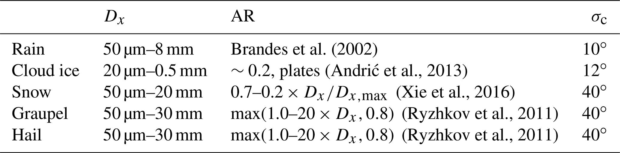
The shape parameters of the Gamma distribution (Eq. 1) and power-law relationship between diameter and particle mass (Eq. 2) for different hydrometeors used in this study are summarized in Table 1. Further, SB2M does not have a prognostic melted fraction, and instantaneously transfers the amount of meltwater formed during one model time step from cloud ice, snow, graupel and hail to the rain class.

Table 1 Hydrometeor parameters for mass-diameter relationship and generalized gamma distribution for the of two-moment microphysics scheme including minimum and maximum values of mean particle mass.

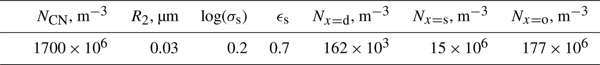
The activation of cloud condensation nuclei (CCN) from aerosols in SB2M is based on precomputed activation ratios stored in a lookup table (Seifert et al., 2012), which depend on the vertical velocity and background aerosol properties (Segal and Khain, 2006). The aerosol is assumed to be partially soluble with a two-mode lognormal size distribution. This requires the specification of the condensation nuclei (CN) concentration, the mean radius of the larger aerosol mode, the logarithm of its geometric standard deviation, and its solubility. The vertical profile of the CN concentration is assumed constant up to 2 km height followed by an exponential decay above. The ice nuclei (IN) number densities of dust, soot and organics are also prescribed for heterogeneous ice nucleation based on the parameterization of Kärcher and Lohmann (2002) and Kärcher et al. (2006). Table 2 summarizes the large-scale aerosol specification for the cloud droplet and ice particle nucleation used in this study. In absence of an prognostic aerosol model, the prescribed values remain constant, and processes like scavenging or chemical transport are not modelled.

Table 2 Large-scale continental aerosol specification for cloud droplet nucleation and default parameters for ice nucleation.

2.2 Forward operator

The Bonn Polarimetric Radar forward Operator (B-PRO; Heinze et al., 2017; Xie et al., 2021; Trömel et al., 2021; Shrestha et al., 2022) used in this study is a polarimetric extension of the non-polarimetric EMVORADO (Zeng et al., 2016) operator, which computes the polarimetric radar variables from scattering amplitude calculations using the T-matrix method (Mishchenko et al., 2000). The synthetic polarimetric moments are output on the spatial grid given by the numerical model field.

B-PRO simulates the polarimetric radar variables at specified weather radar wavelengths (X-band – 3.2 cm) using prognostic model states of temperature, pressure, humidity, wind velocity, mixing ratio and number densities of hydrometeors. Besides cloud liquid class, the hydrometeors are interpreted as homogeneous oblate spheroids in the T-matrix computation. Additional uncertainties in the polarimetric estimates arise from required hydrometeor information usually not available from the model like spheroid diameter (D_x), aspect ratio (AR), width of canting angle distributions σ_c and dielectric constant. The latter is further dependent on hydrometeor density, water content, temperature and liquid–ice-phase partitioning, and a selection of effective medium approximation available for ice–air and water–ice–air mixtures. Since SB2M does not have a prognostic melted fraction, B-PRO uses melting parameterization for treatment of melting hydrometeors. Table 3 summarizes the parameters used to estimate the scattering properties of the modelled hydrometeors in the forward operator. The diameter size distribution f(D_x) is calculated for all hydrometeors based on the estimated parameters of the gamma distribution A and λ (Eq. 1) using the shape parameter (Table 1) and model outputs of q_x and N_x. For rain below clouds (q_c=0), the shape parameter is diagnosed from of q_r and N_r, using the parameterization of the shape of the raindrop size distribution as a function of the mean volume diameter (Seifert, 2008). More details about the B-PRO are also available from Shrestha et al. (2022).

Brandes et al. (2002)(Andrić et al., 2013)(Xie et al., 2016)(Ryzhkov et al., 2011)(Ryzhkov et al., 2011)

Table 3 Assumed hydrometeor physical properties for T-matrix computation in the B-PRO.

Since T-matrix computations are computationally very expensive in the absence of lookup tables, B-PRO simulations are performed only for a cropped model domain ($\mathrm{180}\times \mathrm{180}\times \mathrm{80}$ grid points) and for limited time periods. We also decomposed the model grid area into smaller subdomains ($\mathrm{20}\times \mathrm{20}\times \mathrm{80}$ grid points), such that B-PRO can be run in parallel in order to further speed up the T-matrix computations.

3 Polarimetric radar observations

The observed polarimetric radar variables used in this study are based on the twin research X-band Doppler radars located in Bonn and Jülich (BoXPol and JuXPol; Diederich et al., 2015a, b), which operate at a frequency of 9.3 GHz with a radial resolution of 100–150 m and a scan period of 5 min. Both X-band Doppler radars produce volume scans consisting of a series of plan position indicators (PPIs) measured at 10 different elevations, mostly between 0.5 and 30^∘, followed by a vertical cross section (RHI – range height indicator) in a specific direction and a vertically pointing scan. The use of these multiple PPI sweeps became more popular in recent years in order to get a 3-D picture of surrounding hydrometeors and microphysical processes. These PPIs can be exploited for improved process understanding, model evaluation and data assimilation. And, such volume scans also enable us to construct vertical cross sections of convective systems.

Z_H was calibrated by comparison with observations of the Dual-frequency Precipitation Radar (DPR) aboard the Global Precipitation Mission (GPM) Core Observatory satellite. To this goal, both observations are first brought to the same observational volumes, then the melting layer is identified and excluded from the calculation of the median. The calibration based on GPM DPR (Ku band) is consistent with results obtained with the methodology described in Diederich et al. (2015a). Furthermore, the calibration technique selects only stratiform events where a bright band is visible, and only reflectivities between 10 and 36 dBZ are taken into account, to avoid strong effects of attenuation. Successful calibrations of ground-based radars with satellite-based radars have been also been done in several previous studies (Schwaller and Morris, 2011; Protat et al., 2011; Warren et al., 2018; Crisologo et al., 2018; Louf et al., 2019).

The Z_DR calibration uses vertical scans where near-zero Z_DR are expected. Values with ρ_hv<0.9 are filtered out to avoid impacts of non-meteorological scatterers, and Z_H>30 dBZ are ignored to keep only stratiform events. The melting layer and the near-radar gates (first 600 m) are also removed to reduce noise and the offset calculated as the median of the remaining values (Williams et al., 2013; Ryzhkov and Zrnic, 2019). Further adjustments are made for both Z_H and Z_DR based on a comparison between BoXPol and JuXPol. The radar calibration varies with time; see Table B1 in Appendix B for observed offsets for the different events.

Besides radar miscalibration and partial beam blockage, the polarimetric variables Z_H and Z_DR are affected by (differential) attenuation, especially at smaller wavelengths (C band and X band), and their correction especially in deep convective, hail-bearing cells gives rise to additional uncertainties (Snyder et al., 2010). Corrections for attenuation and differential attenuation especially due to hail follows the algorithm from Ryzhkov et al. (2013). The algorithm first identifies radial segments with potential hail along the beam via Z_H>50 dBZ. For these segments, the coefficient for attenuation is calculated via the ZPHI method from Testud et al. (2000). Differential attenuation due to the presence of hail is calculated by comparing the observed Z_DR behind the hotspot with an expected value based on Z_H (at values between 20 and 30 dBZ) to ensure light rain, Eq. (11) in Ryzhkov et al. (2013) and use the difference to calculate the value of the differential attenuation coefficient in the hail core. For other segments, the standard linear relationships between attenuation and differential attenuation and differential phase (ϕ_DP) are used with standard coefficients for X band from Ryzhkov and Zrnic (2019) (α=0.28 and β=0.03). These coefficients are not used for the hail inflicted segments for which we do not know the actual attenuation and differential attenuation – the above method only provides estimates of attenuation-corrected Z_H and Z_DR.

In contrast, K_DP is not affected by miscalibration and attenuation. However, the total differential phase shift is a combination of backscatter differential phase (δ) and propagation differential phase (φ_DP); thus, the subtraction of the former from the total differential phase shift (Φ_DP) is required before computing K_DP. This is particularly important when hydrometeor sizes are in the range of or larger than the radar wavelength; these so-called resonance effects are most pronounced at C band but also significant at X band (Trömel et al., 2013). Once the contribution of (δ) is removed, K_DP is estimated by calculating the range derivative of φ_DP. We acknowledge this uncertainty in the estimates of attenuation corrected radar observations, and identifying the contribution of (δ) affects, which can affect the K_DP estimates.

Based on the time and location of the storm from the radar, PPI measured at different elevation for each case are used, giving insights of the measurement of convective systems at different heights (∼1 km, near the melting layer and 2–3 km above melting layer). We also further interpolated the polarimetric radar data from the native polar coordinates to cartesian coordinates at 500 m horizontal and vertical resolution using a Cressman analysis with a radius of influence of 2 km in the horizontal and 1 km in the vertical. While, the data in native polar coordinates is used for investigating polarimetric signatures, the gridded data allows for easy comparisons with their model-simulated equivalents. Ground clutter and non-meteorological scatterers are known for having significantly decreased values of ρ_hv compared to precipitation (Zrnic and Ryzhkov, 1999; Schuur et al., 2003). Therefore, a threshold of 0.8 in ρ_hv was imposed in the gridded data to ensure that clutter is filtered out without removing useful meteorological information.

Besides the observations from the X-band radars, the RADOLAN (Radar Online Adjustment; Ramsauer et al., 2018; Kreklow et al., 2020) data from the German national meteorological service (DWD, Deutscher Wetterdienst) is also used for evaluating the modelled precipitation. RADOLAN is a gauge adjusted precipitation product based on DWD's C-band weather radars available at hourly frequency in a spatial resolution of 1 km.

4 Experimental setup

The model evaluation with polarimetric radar data is conducted for three cases of summertime convective storm events producing hail, heavy precipitation and severe winds. Figure 1 shows the synoptic conditions for the three cases; shown are the surface pressure reduced to mean sea level and pseudo-equivalent potential temperature based on GFS analysis at 12:00 UTC. Additional synoptic plots are also directly available from http://www1.wetter3.de (last access: 25 May 2022). The first case (5 July 2015) is a northeastward-propagating deep convective hail-bearing storm crossing Bonn. The storm was associated with a low-pressure system west of Ireland with an occluded front crossing Norway and the cold front extending over the western part of middle Europe producing pre-frontal convergence zones over western Germany, where a moisture tongue ahead of the cold front produced instability and drew warm moist air mass from the south (Fig. 1a). Scattered northeasterly propagating storms were prevalent throughout the day, with an isolated deep convective storm passing directly over the Bonn radar from 15:00 to 16:00 UTC. According to the European Severe Weather Database (ESWD), large hail (2–5 cm in diameter) was observed over the Bonn region, including damaging lightning further north, and heavy precipitation with severe wind (further northeast).

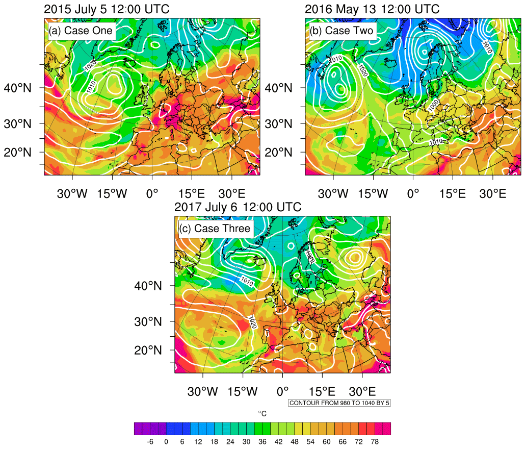
Figure 1 Synoptic conditions for the three different cases – surface pressure reduced to mean sea level and 850 hPa pseudo-equivalent potential temperature. The plots are based on GFS analysis data.

The second case (13 May 2016) is characterized by scattered convective storms over Rhineland-Palatinate, Germany, associated with a low pressure system over the Norwegian sea with an occluded front over northern and a cold front over southern Germany (Fig. 1b). The southward-propagating cold front provided the necessary lift to release the potential instability associated with a warm moist air mass below 700 hPa over the region between the occlusion and the cold front. The ESWD reported heavy rainfall over the Frankfurt area resulting in flooding and damage to property.

The third case (6 July 2017) consists of deep convective clouds propagating eastwards over Bonn. On that day, a warm front over central Germany separated a relatively cool northern, from a warm southern Germany (Fig. 1c). The additional northward push of the warm front produced the necessary lift to release the potential instability associated with the warm and moist southerly air mass. The ESWD reported scattered severe wind around the Bonn region and heavy precipitation south of Mainz including large hail.

4.1 Model domain

The experiment is setup over the Bonn radar domain (Shrestha, 2021a) – a temperate region in the northwestern part of Germany bordering with the Netherlands, Luxembourg, Belgium and France (Fig. 2a). The region has a quite heterogeneous land cover and comprises extensive emissions by point (e.g. oil refineries, photochemical industries) and area sources (e.g. extensive urban and rural areas, road transport, extensive agriculture, railways) (Kulmala et al., 2011; Kuenen et al., 2014). The twin polarimetric X-Band research radars in Bonn (BoXPol) and Jülich (JuXPol) and the overlapping measurements from four polarimetric C-Band radars of the German Weather Service (Deutscher Wetterdienst, DWD) make the region probably the best radar-monitored area in Germany. The model domain covers approximately 333×333 km² area with a horizontal grid resolution of 1.132 km. In total, 80 levels are used in the vertical with a near-surface-layer depth of 20 m for the atmospheric model. For the hydrological model, 30 vertical levels with 10 stretched layers in the root zone (2–100 cm) and 20 constant levels (135 cm) below is used, extending down to 30 m below the surface.

Figure 2 (a) Spatial pattern of topography and extent of Bonn radar domain (solid line) including the coverage of BoXPol and JuXPol (red circles). The dotted lines indicate the inner domain (excluding the relaxation zone) used to compute the domain average precipitation. (b) Spatial pattern of plant functional types (PFTs). Also shown is the coverage of two X-band radars.

The land cover type and associated phenology is based on the Moderate Resolution Imaging Spectroradiometer (MODIS) remote sensing products (Friedl et al., 2010; Myneni et al., 2015). The Rhein massif intersected by the Middle Rhein Valley dominates its topography, and the land cover consists of forested areas (58 %), agricultural land (23 %), urban areas (12 %) and grasslands (7 %).

4.2 Simulations

Ensemble simulations with 20 members for three case studies are used to quantify the meteorological uncertainty in simulated precipitation and polarimetric variables. The hourly model output from the 20 ensemble members of the COSMO-DE Ensemble Prediction System (EPS; Gebhardt et al., 2011; Peralta et al., 2012) provided by DWD is used for the model runs in this study. The COSMO-DE is a high-resolution (2.8 km) configuration of the COSMO model encompassing the entire extent of Germany. The 20 ensemble members of COSMO-DE EPS can be divided into four subsets of five members each. The four subsets represent different global models: the Integrated Forecast System of ECMWF (IFS; ECMWF, 2003), the global model of DWD (GME; Majewski et al., 2002), the Global Forecast System of NCEP (GFS; Center, 2003) and the Unified Model of the UK Met Office (UM; Staniforth et al., 2006), used to vary the boundary conditions of the COSMO-DE. Each subset of the five members is then perturbed by varying a set of parameters that control the physics parameterization of the COSMO model. The general statistics of the EPS are always stratified according to four global models when used for IC/BC perturbations of COSMO-DE; i.e. the five members having the same global model are more similar to each other (personal communication: G. Christoph, DWD). Since January 2015, the ICON (ICOsahedral Non-hydrostatic Zängl et al., 2015) modelling framework was used instead of the global numerical weather prediction model GME (Majewski et al., 2002). Also, the EPS system was switched to BCs based on ICON-EU-EPS and IC perturbations generated by a local ensemble Kalman filter from March 2017 onwards.

The initial soil–vegetation states are obtained from spinups using offline hydrological model runs over the same domain (Shrestha, 2021b). In all runs, a coupling frequency of 90 s is used between the atmospheric and hydrological components, which have a time steps of 10 and 90 s, respectively. The models are integrated over diurnal scale starting at midnight. The atmospheric model output is generated at 5 min intervals, while the hydrological model output is generated at hourly intervals. For the third case, the internal variability in the ensemble members was relatively high in terms of the spatiotemporal distribution of convective storms (probably associated with the switching of the ensemble generator in 2017); thus the output was generated at 15 min intervals over a longer model period in order to allow for a fair comparison with observations and to maintain the same load for synthetic polarimetric processing and data storage.

The ensemble simulation per event required an average of 54 core hours using 456 compute cores on the JUWELS (Jülich Wizard for European Leadership Science) machine at Jülich Supercomputing Centre (JSC). Approximately 540 GB of data were produced per event. For polarimetric variables, only 3-hourly data containing 37 time snapshots were processed for each simulation on a local Linux cluster (CLUMA2), amounting to 220 GB per event.

5 Results

5.1 Accumulated precipitation

First, we examine the model-simulated ensemble precipitation with the RADOLAN data. Figure 3 shows the spatial pattern and frequency distribution of the modelled and observed accumulated precipitation over the Bonn Radar domain for the three case studies. Overall, the spatial pattern of ensemble averaged accumulated precipitation resemble the RADOLAN estimates, but the frequency distribution produced by the ensemble members underestimate high precipitation. For the first case (Fig. 3a), the model-simulated accumulated precipitation is stratified according to four global models used for IC/BC. The members using GME data produce average accumulated precipitation and a frequency distribution for average accumulated precipitation (<30 mm) closest to RADOLAN. The model does, however, underestimate average accumulated precipitation (>30 mm) for all ensemble members as also visible in the spatial pattern of the ensemble averaged accumulated precipitation. While the large-scale extent of the precipitating area is comparable between model and RADOLAN, the precipitation amount especially in the northeastern domain is underestimated. For the second case (Fig. 3b), all ensemble members underestimate the average accumulated precipitation compared to RADOLAN; also its frequency distribution for high precipitation is weaker compared to the first case. All ensemble members for second case, underestimates average accumulated precipitation (>10 mm). For the third case (Fig. 3c), the model misses the precipitation observed over the western part of the domain for all ensemble members except for one, and the simulated frequency distribution of accumulated precipitation exhibits a larger spread. This could be attributed to the switch in the ensemble generator for large-scale atmospheric forcing data.

Figure 3 Spatial pattern and frequency distributions of accumulated precipitation over the Bonn radar domain for three case studies (a, b, c). For each case studies, the left and middle panels show the spatial pattern of accumulated precipitation from model (ensemble average) and observations. The right panel shows the frequency distributions of accumulated precipitation for each ensemble member (dashed light grey line) and observation (dashed black line). The inset in the right panel shows the domain average accumulated precipitation for each ensemble member (light grey colour bar) and observation (black colour bar) with 1 standard deviation (solid line above the bars).

5.2 Polarimetric signatures

For a given precipitation type, polarimetric variables are expected to cluster in a specific region of the multi-dimensional space (Zrnic and Ryzhkov, 1999). Thus as one evaluation method, we compare the respective clustering between simulations and observations for similar stages of convection, which we identify via the convective area fraction (CAF: area fraction of a storm with radar reflectivity >40 dBZ at 2 km height above ground level (hereafter a.g.l.; Fig. 4) and by a qualitative exploratory analysis of the model ensembles and the observed storm evolution. The total area of the storm for CAF estimate, includes the grid points of the storm with radar reflectivity >0 dBZ at 2 km a.g.l. height. The time extent of the CAF evolution was chosen such that the storm is within the domain. However, due to variability in the ensemble members, some members are affected as part of the storm approaches the boundary in the last 30 min of CAF evolution for cases 1 and 2. For case 3, due to extended sampling time used, the CAF is also partly impacted by the storm moving off the grid for the synthetic data. For the first case, the observed storm CAF decreases while approaching the radar and increases again while moving away from the radar. Especially, the ensemble members initiated and forced with GME model (relatively dark lines) show a similar behaviour but underestimate CAF compared to observations. For the second case, CAF gradually increases for all ensemble members and remains quasi-steady after 11:00 UTC. However, all ensemble members underestimate CAF in the earlier phase of the storm (before 11:00 UTC) compared to observations. For the third case, the simulated CAFs of the model ensembles have a wider spread, probably caused by a switch in the way the ensemble is generated from March 2017 onwards. While few ensemble members simulate the storm much earlier than observed (relatively dark lines), the CAF of one ensemble member, better matches the observations and exhibits also a storm evolution (dark line) quite similar to the observations.

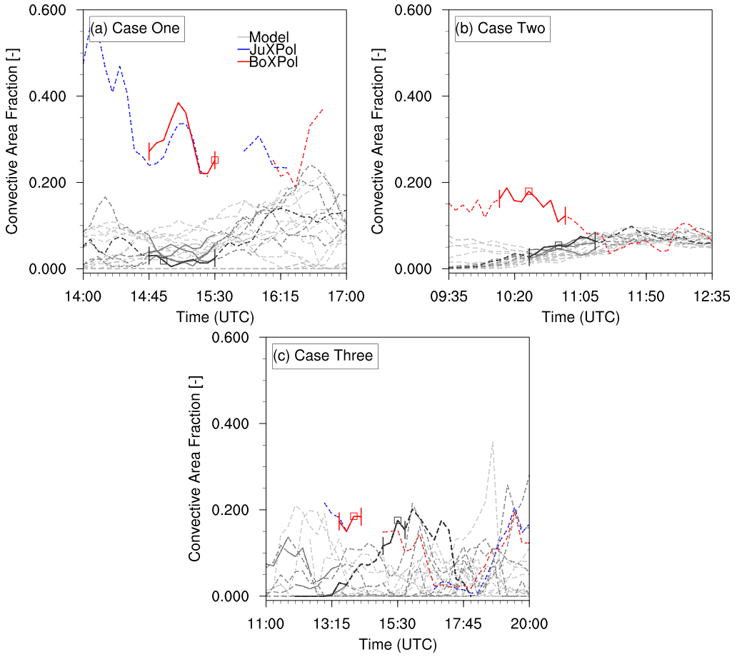
Figure 4 Convective area fraction (CAF) of model ensemble members and observations for the three different case studies. The two vertical bars define the time period used to compute CFADs for observation (red colour) and model (grey colour) with selected ensemble members (solid lines within this extent). The ensemble member with solid black line is used for polarimetric signature comparison. The square marker (red and grey) represents the snapshot used for polarimetric comparison between observation and model for each case study. The observations from BoXPol or JuXPol are shown upon coverage and data availability. The gaps in the radar data represent times, when the polarimetric signatures are strongly attenuated or if the storm extent is only partially covered by the radar.

The comparison of model with observation is always challenging, due to mismatches of the simulated and observed storm evolution in space and time (also shown by the variability in the CAF evolution). So, besides exploring the time series of CAF, we also conducted a qualitative exploratory analysis (using synthetic polarimetric variables at lower levels (∼ 1000 m a.g.l.), middle levels (near the melting layer) and upper levels (2.5 km above melting layer) to find the simulated convective storm among the ensemble members that was closest in time and location compared to the polarimetric observations. Importantly, a qualitative exploratory analysis of the PPIs (at different elevations) and reconstructed RHIs of observed polarimetric variables were also conducted to identify prominent polarimetric signatures. Based on the above two analyses, we identified the ensemble members, time snapshot (identified by square markers in Fig. 4) and time intervals (solid lines bounded by vertical bars in Fig. 4) for the comparison of the polarimetric features and statistical distribution of polarimetric variables between observations and simulations, respectively.

Here, we have to note that both synthetic and observed radar variables are affected by errors in forward operator and calibration/attenuation corrections, respectively. We acknowledge this limitation in the study and concentrate more on the prominent patterns and not so much on the actual magnitudes of the polarimetric variables.

5.2.1 Case 1

Figure 5a shows the PPI plots of Z_H, Z_DR, K_DP and ρ_hv at 8.2^∘ elevation observed by BoXPol at 15:30 UTC for the first case. The storm is characterized by high reflectivity (>50 dBZ) and differential reflectivity (>2 dB) near the melting layer. An arc-like feature of high Z_DR follows the leading eastern edge of the storm just below the melting layer with concurrent lower Z_H values suggesting hydrometeor size sorting associated with storm inflow (Kumjian and Ryzhkov, 2012; Dawson et al., 2014; Suzuki et al., 2018). Figure 5b shows a cross section of storm based on the gridded radar data. Its convective part between −20 and 5 km relative to BoXPol exhibits a notable polarimetric feature – Z_DR columns, anchored to lower levels and extending up to 6 km altitude associated with two strong updraft zones. They are associated with the presence of supercooled raindrops, water-coated hail growing in a wet growth regime and frozen raindrops aloft, and their different extensions suggest different updraft intensities (Kumjian and Ryzhkov, 2008; Kumjian et al., 2014; Snyder et al., 2015). K_DP columns (Ryzhkov and Zrnic, 2019; Snyder et al., 2017b) co-located with the Z_DR columns are another prominent polarimetric feature with slight inward offsets that are considered additional signs for updraft locations and presence of liquid water associated with either supercooled raindrops or water-coated hail (van Lier-Walqui et al., 2016). The low (<0.7) cross-correlation coefficient (ρ_hv) near the inflow region and the even lower ρ_hv (<0.92) along the strong convective core associated with high reflectivity probably indicates hail. The dominance of near-zero Z_DR and reflectivity values between 20 and 25 dBZ above the melting layer in the downdraft region suggest the dominance of snow (Yuter and Houze, 1995). The low ρ_hv in the northern region at higher levels associated with relatively high Z_DR and moderate K_DP is probably caused by horizontally oriented ice crystals.

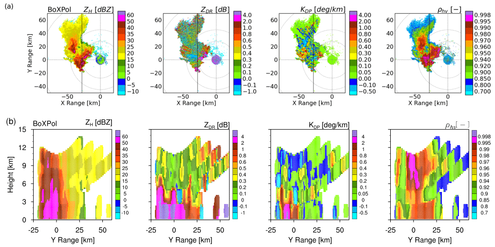
Figure 5 (a) PPI plots of horizontal reflectivity, differential reflectivity, specific differential phase and cross-correlation coefficient at 8.2^∘ elevation measured by BoXPol on 5 July 2015 at 15:30 UTC. The dotted grey circles represent slant ranges for the chosen elevation angle, associated with heights of 1 km (lower levels), 4.5 km (melting layer) and 7 km (upper levels). (b) Cross section of the same polarimetric variables from the gridded data. The vertical solid black line along the y axis in panel (a) indicates the location of cross-section plots.

As discussed in Sect. 5.1, the ensemble members initiated using GME data have similar storm evolutions as observed. So, only these ensemble members are used here for the polarimetric comparisons. Figure 6 shows the synthetic polarimetric moments at lower levels up to the melting layer and cross sections of polarimetric variables and simulated hydrometeors at 14:55 UTC for one of the ensemble members (Fig. 4a – dark solid line). At lower levels (1000 m a.g.l.), the southeastern flank of the storm has – as expected near the core of the storm – relatively high Z_H and Z_DR (also associated with relatively low ρ_hv) with lower magnitudes on the northwestern side. K_DP has generally low magnitudes, while ρ_hv is generally high. Near the melting level (4000 m a.g.l.), K_DP present much lower magnitudes but a ring-like feature in Z_DR with relatively low ρ_hv is visible in the convective core, which is a typical polarimetric feature found for supercell storms (Kumjian and Ryzhkov, 2008). This enhanced Z_DR found in observations are hypothesized to be contributed by ice-phase hydrometeors upon melting or accretion of liquid water (Ryzhkov and Zrnic, 2019). Here, the synthetic elevated Z_DR is primarily contributed by the elevated perturbation of warm temperature in the convective core and the melting of ice-phase hydrometeor, which is parameterized in the FO.

Figure 6 (a, b) Model-simulated horizontal reflectivity, differential reflectivity, specific differential phase and cross-correlation coefficient at low level (1000 m a.g.l.) and near the melting layer (4000 m a.g.l.) on 5 July 2015 at 14:55 UTC. The “×” symbol refers to the BoXPol location. The solid grey line indicates the location of cross section. (c) Cross section of the same polarimetric variables. (d) Cross section of model-simulated hydrometeor density – QR (rain), QI (ice), QS (snow), QG (graupel) and QH (hail). Also shown are the 0 ^∘C line (solid black line) indicating the melting layer, contours of vertical velocity [5, 40 m s⁻¹] with QS and contours of the QH with QG.

In all ensemble members, the storm is aligned in the northeast direction and has a strong updraft region in the southeastern edge characterized by a bounded weak echo region (BWER; see Fig. 6c). The convective storm top extends up to 15 km height with Z_H between 30 and 40 dBZ (which is relatively lower than the observed Z_H) co-located with the simulated hail shaft and updraft (Fig. 6d). The model also exhibits a narrow Z_DR column-like feature extending up to 6 km altitude in the convective core. However, the simulated Z_DR column is relatively smaller in width and magnitude (value) compared to the observations. The synthetic Z_DR column signature is a result of supercooled raindrops with mean diameter size of 1.3–1.7 mm. The model also simulates high K_DP (>1^∘ km⁻¹) along the top of the convective storm part, but no K_DP columns are present adjacent to the updraft region above the melting layer as seen in the observations. Although, the simulated ρ_hv is higher than observed, a slight decrease can be observed in the updraft region with high Z_H associated with hail, in the Z_DR column and below the melting layer. In the updraft region, the modelled vertical velocity above 8 km reaches 40 m s⁻¹, dominated mostly by supercooled raindrops around 6–9 km (see Fig. 6d), which is an important source for hail growth. The strong updraft also generates a warm anomaly above the melting layer (see the 0^∘ isotherm) in the simulations, below which rain is also formed by the melting of graupel and hail. Graupel dominates the frozen hydrometeor categories above the melting layer peaking at the top of the updraft region. Ice crystals are located mostly above 8 km height, and the self-collection of these ice particles leads to the formation of snow which further grows in size via aggregation. Hail is present in low concentration in the convective core but contributes dominantly in the polarimetric signals in terms of high reflectivity, Z_DR (especially below the melting layer) and lower ρ_hv.

5.2.2 Case 2

Figure 7 shows the PPIs of Z_H, Z_DR, K_DP and ρ_hv at 1.0^∘ elevation from BoXPol at 10:30 UTC for the second case. We find moderate reflectivities (35–40 dBZ) and high Z_DR (>2 dB) at around 1 km. According to the cross section of storm based on gridded polarimetric radar data (Fig. 7b), the storm has a wide Z_DR column-like feature anchored to the lower levels and extending up to 5 km. At this location, below the melting layer (approximately 2.5 km), Z_DR is >2 dB while reflectivity is weak, which suggests size sorting of raindrops. A large portion of the storm exhibits very low or negative Z_DR above the melting layer, possibly indicating vertically oriented or conical graupel (Bringi et al., 2017). While other studies also have shown the presence of low and negative Z_DR above the melting layer for convective storms (Suzuki et al., 2018; Hubbert et al., 2018), it is possible that for these convective cases, attenuation correction even with the advanced methods as we used here may at least partially contribute to negative Z_DR.

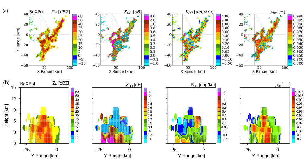
Figure 7 (a) PPI plots of horizontal reflectivity, differential reflectivity, specific differential phase and cross-correlation coefficient at 1.0^∘ elevation measured by BoXPol on 13 May 2016 at 10:30 UTC. The dotted grey circles represent slant ranges for the chosen elevation angle, associated with height of 1 km (lower levels). (b) Cross section of the same polarimetric variables from the gridded data. The vertical solid black line along the Y range in panel (a) indicates the location of cross-section plots.

Figure 8 (a, b) Model-simulated horizontal reflectivity, differential reflectivity, specific differential phase and cross-correlation coefficient at low level (1000 m a.g.l.) and near the melting layer (3300 m a.g.l.) on 13 May 2016 at 10:50 UTC. The “×” symbol refers to the BoXPol location. The solid grey line indicates the location of cross section. (c) Cross section of the same polarimetric variables. (d) Cross section of model-simulated hydrometeor density – QR (rain), QI (ice), QS (snow), QG (graupel) and QH (hail). Also shown are the 0 ^∘C line (solid black line) indicating the melting layer, contours of vertical velocity [5, 40 m s⁻¹] with QS and contours of the QH with QG.

Figure 8a–b show the synthetic polarimetric moments up to near the melting layer and cross sections of polarimetric variables and simulated hydrometeors at 10:50 UTC for one of the ensemble members (see Fig. 4b – thick solid line). The southward-propagating storm is oriented in the north–south direction. Regions with moderate-to-high reflectivities in the lower levels (1000 m a.g.l.) coincide with moderate to high Z_DR, K_DP and lower ρ_hv suggesting heavy rain or rain/hail mixtures. Just above the melting level (3000 km a.g.l.), Z_DR and K_DP are much lower except on the western storm edges, where slightly enhanced Z_DR and K_DP features are found. According to the cross section (Fig. 8c), moderate reflectivities (30–50 dBZ) comparable to the observations, reach up to 6 km height, while the storm top height extends up to 9 km. The model does not capture a distinct Z_DR column but simulates narrow region with enhanced Z_DR and lower ρ_hv above the melting layer, extending up to 7 km (Fig. 8d). The simulated enhanced Z_DR is due to the presence of supercooled raindrops with mean diameter size of 0.7–0.9 mm. A grid-scale enhanced K_DP extending up to 4 km above the melting layer is also visible but K_DP generally, remains very low here except for some regions near the storm top, which is also visible in the observations.

Based on the modelled hydrometeors, Fig. 8d indicates presence of supercooled raindrops above the melting layer connected with updraft regions (5 m s⁻¹ maximum vertical velocity at the left and right edges of the storm). However, the smaller sizes of raindrops (<1 mm) are not sufficient to create strong Z_DR magnitudes as observed in the Z_DR columns. The vertical velocity in the storm centre is around 1 m s⁻¹ and not included in the contour plot. The frozen hydrometeors are again dominated by graupel with high concentrations in the strong updraft region. Hail is present in low concentrations, adjacent to the updraft regions reaching down to the surface. Above 6 km height, some cloud ice exists, while this region is mostly dominated by snow.

5.2.3 Case 3

Figure 9 shows the PPIs of Z_H, Z_DR, K_DP and ρ_hv at 8.2^∘ elevation from BoXPol at 14:00 UTC. The storm is characterized by reflectivities >50 dBZ and Z_DR>2 dB near the melting layer. Its convective region (“reflectivities” > 50 dBZ) extends up to 12 km height and the corresponding lower ρ_hv indicate presence of hail (Fig. 7b). The convective core has also relatively high K_DP values extending up to the storm top and including a wide Z_DR column up to 5 km height. Both indicate lofting and growth of large raindrops by updrafts, which are also important for hail formation. This case also shows low to negative Z_DR values above the melting layer, which could also be partially contributed by limitations on the attenuation correction algorithm.

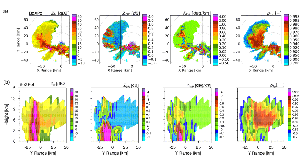
Figure 9 (a) PPI plots of horizontal reflectivity, differential reflectivity, specific differential phase and cross-correlation coefficient at 8.2^∘ elevation measured by BoXPol on 6 July 2017 at 14:00 UTC. The dotted grey circles represent slant ranges for the chosen elevation angle, associated with a height of 1 km (lower levels), 4 km (melting layer), 6.5 km (upper levels) and 13 km. (b) Cross section of the same polarimetric variables from the gridded data. The vertical solid black line along the Y range in panel (a) indicates the location of cross-section plots.

Figure 10 (a, b) Model-simulated horizontal reflectivity, differential reflectivity, specific differential phase and cross-correlation coefficient at low level (1000 m a.g.l.) and near the melting layer (4000 m a.g.l.) on 6 July 2017 at 15:30 UTC. The “×” symbol refers to the BoXPol location. The solid grey line indicates the location of the cross section. (c) Cross section of the same polarimetric variables. (d) Cross section of model-simulated hydrometeor density – QR (rain), QI (ice), QS (snow), QG (graupel) and QH (hail). Also shown are the 0 ^∘C line (solid black line) indicating the melting layer, contours of vertical velocity [5, 40 m s⁻¹] with QS and contours of the QH with QG.

Figure 10 shows the plan view of synthetic polarimetric variables (at lower levels and near the melting layer) and a cross section of them including hydrometeors at 15:30 UTC simulated by one of the ensemble members (see Fig. 4c – thick solid line). The eastward-propagating storm is oriented from west to east and at lower levels characterized by a wide core of moderate reflectivity (40–50 dBZ) and high K_DP, Z_DR>2 dB along the edges and low ρ_hv produced by heavy rain and rain/hail mixtures. Near the melting level (4000 m a.g.l.), variable Z_DR and Z_H features are found near the southeastern edge – characteristics of raindrop size sorting. Overall, Z_DR and K_DP are low throughout the storm. According to the cross section (Fig. 10c), the storm extends up to 12 km with moderate reflectivities (30–50 dBZ). While Z_H at lower levels is comparable to observations, the relatively high Z_H seen in the observations extending up to upper levels is underestimated by the model. The model also simulates a narrow Z_DR column extending up to 5 km adjacent to the updraft region and relatively comparable to observation. The Z_DR column signature is a consequence of supercooled raindrops with mean diameter size of 1.7–1.9 mm. The convective core also has relatively higher Z_DR than the background, extending up to 12 km height. The model also simulates high K_DP along this convective part of the storm. The simulated ρ_hv is again generally high with slight decrease in the convective core and below the melting layer, an indication of hail, together with the high Z_H. Similar features of Z_DR, K_DP and ρ_hv are also seen in the observed convective core.

The vertical velocity reaches to 10 m s⁻¹ from 6–11 km in the updraft region where a low concentration of supercooled raindrops is found up to 8 km (Fig. 10d). Graupel again dominates the frozen hydrometeor categories above the melting layer, while snow further extends downwards up to 6 km height. Compared to the other two cases the simulated hail concentration is relatively higher and contributes dominantly to the polarimetric signatures.

5.3 Frequency distribution of polarimetric variables

Because mismatches between space and time scales of synthetic polarimetric moments compared to observations are present, ensemble properties of the convective event are also monitored. For this purpose, the ensemble simulations are compared to the observations for similar storm evolution stages using contoured frequency altitude diagrams (CFADs; Yuter and Houze, 1995) using the same extents and bin widths for observations and simulations.

5.3.1 Case 1

We use the observations from 14:45 to 15:30 UTC, which encompasses the convective stage of the storm before it passes over the BoXPol. The CFADs from the X-band radar (Fig. 11a) show a unimodal distribution of Z_H which gradually narrows above the melting layer (around 4 km). The peak in the frequency distribution occurs around 20–25 dBZ with maximum reflectivities well above 50 dBZ. The Z_DR also exhibits a unimodal distribution which further peaks (or narrows) above the melting layer with the mode around 0.25 dB, similar to the values reported by Yuter and Houze (1995) for convective storms. The distribution broadens and shifts to values up to 4 dB below the melting layer peaking at around 1 dB near the surface. K_DP exhibits a unimodal distribution throughout the vertical extent of storm with peak values around 0.1^∘ km⁻¹. The distribution also broadens weakly from 7 km height downwards. ρ_hv has a quite broader distribution peaking around 0.98 below 11 km height and shifting to 0.87 near the storm top.

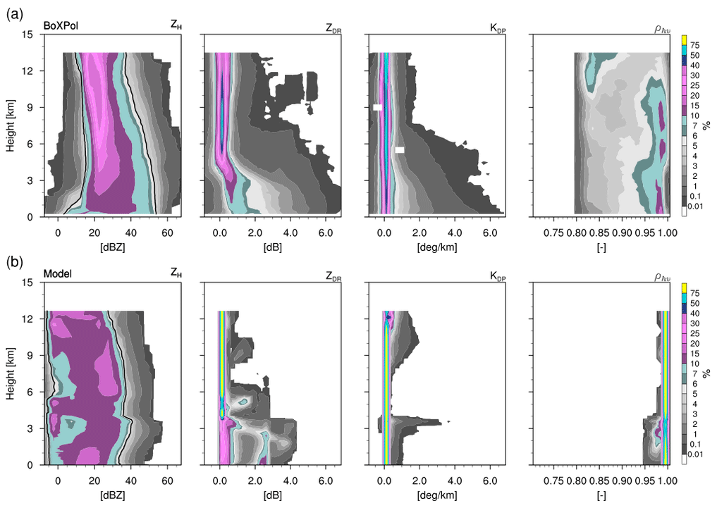
Figure 11 CFADs of horizontal reflectivity, differential reflectivity, specific differential phase and cross-correlation coefficient from 14:45 to 15:30 UTC on 5 July 2015. CFADs from the model are shown for five ensemble members.

The CFADs from the model ensemble were generated using five members from 14:45 to 15:30 UTC (Fig. 4a – solid lines) which best matched the observed storm macrophysical features. The Z_H distribution with maximum reflectivities generally below 50 dBZ peaks around 28 dBZ from 6 to 10 km, but shifts towards 15–20 dBZ at lower levels, which were found to be associated with grid cells with very low concentration of hydrometeors broadening the distribution, compared to observations. Z_DR again exhibits a narrow unimodal distribution above melting layer peaking around 0.1 dB, which broadens below the melting layer with an additional peak at 2.6 dB. Unlike the unimodal CFADs from observations, the CFADs from the model ensemble produce bimodal peaks below the melting layer. K_DP shows a very narrow unimodal distribution compared to the observations with peak values around 0.1^∘ km⁻¹. For the given range (0.7–1.0) of ρ_hv, the frequency distribution appears to be poorly simulated by the model.

5.3.2 Case 2

CFADs are generated during the convective period of the storm from 10:10 to 10:55 UTC. The Z_H observations (Fig. 12a) show a unimodal distribution peaking around 25 dBZ and gradually narrowing above the melting layer (∼3 km) with maximum reflectivities >45 dBZ. Z_DR also exhibits a unimodal distribution peaking above the melting layer at around −0.12 dB but broadening and shifting to higher values with peaks around 0.4 dB near the surface and maxima >2 dB below the melting layer. Compared to case 1, a leftward shift can be observed for the Z_DR distribution, which is primarily caused by domination of low to negative Z_DR above the melting layer. But, similar to the first case, K_DP has a unimodal distribution throughout the storm with peak values around 0.1^∘ km⁻¹ with a very weak broadening downwards and below the melting layer. ρ_hv exhibits again a broader distribution peaking around 0.97 (below 7 km height) and shifting to 0.85 near the storm top.

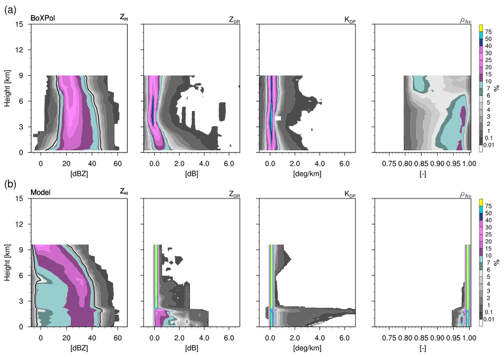
Figure 12 CFADs of horizontal reflectivity, differential reflectivity, specific differential phase and cross-correlation coefficient from 10:10 to 10:55 UTC on 13 May 2016. CFADs from the model are shown for five ensemble members from 10:30 to 11:15 UTC.

The CFADs from the model ensemble were generated from five members from 10:30 to 11:15 UTC (see Fig. 4b – solid lines). The CFADs for Z_H have a broader distribution compared to observation with maxima generally below 45 dBZ; the distribution peaks around 28 dBZ near the melting layer (around 3 km) and gradually shifts towards 10 dBZ near the storm top (around 8 km) and towards 32 dBZ below the melting layer. Z_DR has a narrow unimodal distribution above the melting layer peaking around 0.12 dB. The CFAD broadens below the melting layer with an additional peak at 2.5 dB. Again, the model CFADs produce bimodal peaks compared to unimodal distribution for observations. Additionally, no leftward shift in the Z_DR distribution is observed for model ensembles as seen in observations compared to case 1. K_DP also shows a very narrow unimodal distribution compared to the observations, peaking around 0.12^∘ km⁻¹. The distribution weakly broadens below the melting layer and at upper levels. For the given range (0.7–1.0) of ρ_hv, the frequency distribution again appears to be poorly simulated by the model.

5.3.3 Case 3

CFADs are generated from 13:30 to 14:15 UTC. The observed unimodal Z_H distribution (Fig. 13a) has maxima >50 dBZ and a peak around 25 dBZ which gradually narrows above the melting layer around 4 km and shifts to smaller values peaking around 17 dBZ upwards above 9 km. Z_DR also exhibits again a unimodal distribution above the melting layer with peak around −0.12 dB. The distribution broadens and shifts to larger values below the melting layer peaking around 0.4 dB near the surface with maxima >2 dB. The Z_DR distribution is similar to case 2. K_DP again exhibits a unimodal distribution with peak values around 0.1^∘ km⁻¹ and weakly broadens below the melting layer. Again, ρ_hv has a broad distribution peaking around 0.98 (below 8 km height) but shifting towards 0.83 at the storm top.

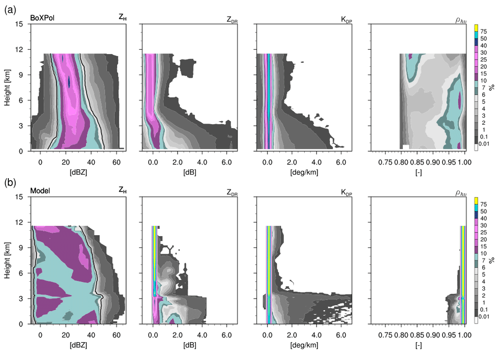
Figure 13 CFADs of horizontal reflectivity, differential reflectivity, specific differential phase and cross-correlation coefficient from 13:30 to 14:15 UTC on 13 May 2016. CFADs from the model are shown for one ensemble member from 15:00 to 15:45 UTC.

The CFADs from the model ensemble were generated using only one ensemble member from 15:00 to 15:45 UTC (see Fig. 4c – solid line) due to strong variability among the ensemble members. The CFADs for horizontal reflectivity have maxima below 50 dBz and again exhibit a broader distribution compared to observations, peaking around 8 and 38 dBZ near the melting layer (around 4 km) producing two peaks, and shift towards 10 dBZ near the storm top (around 10 km) and towards 42 dBZ near the surface. Z_DR has a narrow unimodal distribution above the melting layer with a peak around 0.1 dB and broadens below the melting layer with an additional peak at 1.5 dB. The model again produces bimodal peaks below the melting layer and additionally do not show any leftward shift in the Z_DR distribution as seen between observations for cases 3 and 1. K_DP also shows again a very narrow unimodal distribution with peak values around 0.1^∘ km⁻¹ which broadens both below the melting layer and at upper levels. For ρ_hv, the frequency distribution again appears to be poorly simulated by the model.

6 Discussion

The variability in the lateral boundary conditions for the ensemble members was found to generate probabilistic forecast in the accumulated precipitation and convective area fraction (Gebhardt et al., 2011). The lateral boundary conditions affect the simulated cloud microphysical and macrophysical processes and hence the synthetic polarimetric variables. However, the magnitude of this influence varies between the three studied cases. Particularly, the switch in the ensemble generation for the third case produced a much stronger variability in the spatiotemporal structure of the simulated storm. The CAFs from observations and model simulations indicate that the initial intensity of storms are underestimated by the model, which partly explains the underestimation of high precipitation for all ensemble members. In simulations by Noppel et al. (2010) for a hail storm over southwestern Germany using the same atmospheric model COSMO with the two-moment microphysics, the continental CN concentration (1700 cm⁻³) led to a weaker storm and less surface precipitation compared to maritime CN concentrations (100 cm⁻³). However, their additional sensitivity study by varying the fixed parameters in Eq. (1) for cloud hydrometeors in order to produce a narrow distribution led to a different conclusion, indicating a missing feedback between the CN concentration and the shape parameters of the cloud droplet size distribution (which are both fixed in the model). This mechanism could also be partly contributing to the weaker initial intensity of the storms presented in this study.

The polarimetric radar observations for the three case studies of summertime convective storms exhibits a prominent Z_DR and K_DP columns indicating convective updrafts. In general, the synthetic radar data shows that the model is able to capture the prominent polarimetric signature of the observed convective storms like the Z_DR columns, besides other additional signatures (e.g. size sorting and the ring like feature of Z_DR with relatively lower ρ_hv typically observed in supercells). However, the distinct K_DP columns observed especially in cases 1 and 3 are not captured by the model. Further, a relatively enhanced Z_DR compared to the background is also captured by the model in the convective core for all case studies, which is also present in the observations. While the synthetic Z_DR column for case 3 was close in magnitude to the observed radar data, the model was found to generally underestimate the width and the magnitude (value) of the Z_DR column and its anchorage to the ground, compared to observations. The synthetic Z_DR column signature is a result of the supercooled raindrops only. The missing treatment of freezing raindrops (which do require an additional hydrometeor class) could also be contributing to deficiency in the polarimetric signature (Kumjian et al., 2014). And, to a certain extent, the absence of polarimetric signature contribution from wet growth of hail, which is not parameterized in the FO could additionally be contributing to the deficiency in the shape and magnitude of the synthetic Z_DR column. Besides, the mean diameter size of the raindrops strongly control the magnitude of polarimetric signature. A reason for relatively small mean diameter size of supercooled raindrops could be due to high CN concentrations and the missing feedback between the CN concentration and shape parameters of cloud drop size distribution (Noppel et al., 2010). A sensitivity study with low CN concentrations for case 1 in fact produced high hail concentration, which increased the CAF, Z_DR and Z_H magnitudes of the storm (Trömel et al., 2021).

Below the melting layer in the downdraft regions, where the melting of graupel and hail are the main source of rain water and produce high Z_DR, simulations generally replicate the observations. Above the melting layer, the partitioning of the ice water content in the model is generally dominated by graupel for all case studies. The dominance of graupel has also been reported in previous modelling studies (Pfeifer et al., 2008; Tao et al., 2011; Lang et al., 2011; Shrestha, 2011; Shrestha et al., 2015). For example, similar finding to this study was also reported earlier by Pfeifer et al. (2008) for a squall line over Germany, where they showed that the simulated ice-phase hydrometeors were mostly dominated by graupel, while the observation showed the dominance of snow. In this study, also, case 1 with near-zero Z_DR and reflectivities between 20–25 dBZ, indicate domination of snow in the downdraft region. However, low to negative Z_DR above the melting layer for cases 2 and 3 possibly indicate domination of graupel, but we cannot be completely certain as it might be partially affected by the attenuation correction algorithm as discussed above.

The statistical properties of the observed polarimetric variables exhibit similar patterns for all three case studies in terms of CFADs. In general, the Z_H CFADs from the observations exhibit narrow unimodal distributions peaking around 20–25 dBZ, but differ in maximum reflectivities (>50 dBZ for cases 1 and 3, >45 dBZ for case 2). Similarly, the observed CFADs for Z_DR also show unimodal distribution above the melting layer, which gradually shifts towards higher value near the surface for all three cases. While the pattern of Z_DR CFADs is similar for observations in all cases, the location of the peaks above the melting layer differ between case 1 (0.25 dB) and other two cases (−0.12 dB). This difference in the peak of the observed Z_DR distribution could also point towards the possible difference in partitioning of ice water content above the melting layer as well as partial effect of attenuation correction algorithm. The K_DP CFADs exhibit a narrow unimodal distribution for all case studies, while ρ_hv CFADs exhibit a broader distribution with peak around 0.97–0.98, which shifts towards 0.83–0.87 near the storm top for all cases.

The models do capture the statistical properties of the observed polarimetric variables to a certain extent, but the comparison also outlines many deficiencies in the synthetic polarimetric variables. The Z_DR CFADs from the ensemble simulations exhibit narrow distributions with peak values near zero above the melting layer, which does not differ among the three case studies. It also exhibits bimodal peaks below the melting layer compared to unimodal distribution in observations. Similar bimodal CFADs were also reported by Matsui et al. (2019) for a simulated mesoscale convective system over Southern Great Plains, USA, using both spectral bin microphysics and single-moment cloud microphysics scheme, while the observed CFADs of Z_DR exhibited a more smooth gradient below the melting layer as shown for the observation in this study as well. In their study, even sensitivity studies with FO parameters also could not reproduce the distribution similar to the observations, while producing different results for the two microphysics schemes. In this study, the model tends to strongly underestimate the maximum reflectivities for case 1 but generally it exhibits a broader distribution of Z_H for all three cases compared to the observations, with a peak around 30 dBZ above the melting layer. This higher reflectivity is caused by the dominance of graupel as discussed above. Consequently, the precipitation production by melting of graupel/hail below the melting level, as shown in the cross sections of model-simulated hydrometeors for all cases, could explain the second Z_DR peak at approximately 2 dB in the lower levels. This possibly indicates that the modelled mechanism of precipitation formation below the melting layer differs from the observation. Furthermore, the use of a functional form of drop size distribution in the FO leading to a unique mapping between modelled quantities and synthetic polarimetric quantities can create errors (Kumjian et al., 2019), which could also be partly contributing to this bimodal peak behaviour in the synthetic Z_DR CFADs. Both the ensemble model runs and the observations produce unimodal distribution for K_DP peaking around 0.1^∘ km⁻¹. However, the model again exhibits a narrower distribution above the melting layer compared to observation. Thus, the observed variability in Z_DR and K_DP above the melting layer is underestimated in the synthetic polarimetric variables. Part of this reduced variability can be explained by the deficiencies of the forward operator. Earlier, an extensive sensitivity study with the hydrometeor parameters in the same FO was conducted for a stratiform case over the same modelling domain (Shrestha et al., 2022). In their study, the model was found to exhibit a low bias in the polarimetric moments above the melting layer, where snow was found to dominate, but none of the alternative shape and orientation setups for snow could provide sufficiently strong polarimetric signals to reproduce observed signals at these heights. The inability to reproduce the polarimetric characteristics of snow with T-matrix also justifies the need for a scattering database. This issue needs to be revisited with more sophisticated forward operators available in the future (already planned in this project). For ρ_hv, the CFADs are poorly simulated by the model, probably due to the shortcomings in forward operator assumptions on diversity of hydrometeor shapes and orientation (Shrestha et al., 2022). Although the synthetic ρ_hv exhibits very homogeneous high values above the melting layer, it does exhibit slightly reduced magnitude in locations with elevated Z_DR. This pattern was found to consistent for all simulated case studies.

7 Conclusions

The TSMP model – in particular its atmospheric component COSMO with two-moment cloud microphysics scheme – was found to generally underestimate the initial intensity of storms in terms of convective area fraction, extreme reflectivities. These underestimations were also reflected in the frequency distribution for high precipitation and also broader distribution of reflectivities. The model and FO were able to capture dominant polarimetric feature like Z_DR column but underestimated its width/magnitude compared to observations and could not capture the co-located K_DP columns. Compared to observations, the model was able to simulate similar statistical distribution of Z_DR and K_DP but with less variability above the melting layer, while exhibiting bimodal distribution for Z_DR below the melting layer. The observations also additionally exhibited shifts in the peak of the Z_DR above the melting layer, which was not captured in the model simulations. This shift in the observations, could be associated with differences in partitioning of ice water content above the melting layer as well as the partial effect of attenuation correction algorithm.

The discrepancy between the observed and synthetic polarimetric feature could be attributed to the deficiency in the two-moment cloud microphysics scheme, forward operator and to a certain extent the attenuation correction algorithm or the radar data. Particularly, the model exhibits more graupel for all simulations, which also affects the precipitation production mechanism below the melting layer. While there is a strong understanding of polarimetric signatures for the raindrops, the mechanism by which the raindrops are produced and how the drop size distribution evolves, adds additional uncertainty.

For the two-moment cloud microphysics scheme, the fixed CN concentrations and shape parameters of cloud drop size distribution could also be partly responsible for the overall too low storm intensities, thus regional measurements of CN $/$ IN concentrations, surface precipitation and polarimetric radar data observations could be used together to constrain the shape parameters of cloud droplets. While regional measurements of CN $/$ IN concentrations might not be readily available, sensitivity study with large-scale aerosol perturbations or use of prognostic aerosol/trace gases module could be a way forward to minimize the uncertainty in polarimetric signatures due to aerosols.

On the forward operator for two-moment cloud microphysics scheme, the water content of the ice hydrometeors can strongly modulate the dielectric constant and hence the scattering properties. This information is not directly available in the forward operator – and the melting parameterization in the FO does not completely compensate for the scattering properties of the ice hydrometeors above the melting layer. So, future advancement in the FO should include parameterization for determining more accurate water content of the ice hydrometeors above the melting layer, which would help in obtaining more accurate dominant polarimetric signatures.

Importantly, prominent polarimetric signature of convective storms like the Z_DR column appears to be poorly resolved at kilometre-scale simulations. Future model evaluations with polarimetric radar data should focus on hyper-resolution simulations to better resolve the three-dimensional motion and microphysical processes associated with multivariate polarimetric signatures as well as uncertainty estimates in the attenuation correction of polarimetric moments for convective cases.

Appendix A: Abbreviations

A1 Aerosol specification

Ncn	CN concentration [m−3]
R2	Mean radius of the dominant mode of the aerosol size distribution [µm]
log (σs)	Logarithm of the geometric standard deviation of aerosol
ϵs	Solubility of aerosol
$N_{x=\mathrm{d},\mathrm{s},\mathrm{o}}$	Ice nuclei concentration for dust (d), soot (s) and organics (o) [m−3]

A2 Models

TSMP	Terrestrial Systems Modelling Platform (COSMO, CLM and ParFlow coupled using OASIS3-MCT)
EMVORADO	Efficient Modular Volume Scan Radar Operator
B-PRO	Bonn Polarimetric Radar Forward Operator
COSMO	Consortium for Small-scale Modeling
COSMO-DE	High-resolution (∼2.8 km) configuration of the COSMO model over Germany (DE)
COSMO-DE EPS	COSMO-DE Ensemble Prediction System
CLM	NCAR Community Land Model
ParFlow	Parallel Flow hydrologic model

OASIS3-MCT	Ocean Atmosphere Sea Ice Soil, version 3.0 – Model Coupling Toolkit
IFS	Integrated Forecast System of ECMWF
GME	Global Model of DWD
GFS	Global Forecast System of NCEP
UM	Unified Model of the UK Met Office

A3 Polarimetric variables

δ	Backscatter differential phase
ΦDP	Total differential phase shift
ρhv	Cross-correlation coefficient between horizontally and vertically polarized return signals
σc	Width of canting angle distribution (the canting angle is the angle between the horizontal and the symmetry axis of the falling particles (horizontally aligned particles have a 0∘ canting angle). In a radar-observed volume containing several particles, canting angles vary from particle to particle giving rise to a distribution. The width of the canting angle distribution is a measure of the variability of canting angles in that sample.)
φDP	Propagation differential phase shift
AR	Aspect ratio (ratio between the horizontal and the vertical dimensions of the particle)
Dx	Equivalent/maximum diameter of spherical/non-spherical particles
KDP	Specific differential phase [∘ km−1]
ZDR	Differential reflectivity [dB] (ratio of reflectivity for horizontal and vertical polarization in linear units)
ZH	Reflectivity for horizontal polarization [dBZ]

Appendix B

Table B1 Estimated biases for Z_H and Z_DR for both radars and for each event.