the Creative Commons Attribution 4.0 License.
the Creative Commons Attribution 4.0 License.
 | 08 Jun 2022
Momentum fluxes from airborne wind measurements in three cumulus cases over land
Louise Nuijens
Christian Mallaun
Benjamin Witschas
Christian Lemmerz
Measurements of wind and momentum fluxes are not typically at the centre of field studies on (shallow) cumulus convection, but the mesoscale organization of convection is likely closely tied to patterns in wind. This study combines in situ high-frequency turbulence measurements from a gust probe onboard a Cessna aircraft with downward profiling Doppler wind lidar (DWL) measurements onboard a Falcon aircraft to study variability in the wind profile and momentum fluxes in regions of convection. The dual-aircraft measurements were made during three prototype flights in shallow convective regimes over German agricultural areas (two of which had hilly topography, one flat) in late spring 2019, including forced cumulus humilis under weak winds and “popcorn” cumuli during stronger wind and wind shear after front passages.
All flights show pronounced meso-gamma (2–20 km) scale variability in the wind, with the largest wind variance (on the order of 2–4 m2 s−2) towards cloud base and in the cloud layer on flights with large vertical wind shear. The wind and wind variance profiles measured in situ and by lidar compare very well, despite the DWL's coarse (∼ 8 km) horizontal footprint. This highlights the presence of wind fluctuations on scales larger than a few kilometres and that wind lidars can be used more deliberately in field studies to map (mesoscale) flows.
Cloudy transects are associated with more than twice the momentum flux compared with cloud-free transects. The contribution of the updraft to the total momentum flux, typically one-third to two-thirds, is far less than the typical contribution of the updraft to buoyancy flux. Even on the same flight day, momentum flux profiles can differ per track, with one case of counter-gradient momentum transport when the updraft does carry substantial momentum flux. Scales beyond 1 km contribute significantly to the momentum flux and there is clear evidence for compensating flux contributions across scales. The results demonstrate that momentum flux profiles and their variability require understanding of motions across a range of scales, with non-negligible contributions of the clear-sky fluxes and of mesoscales that are likely coupled to the convection.
Please read the corrigendum first before continuing.
-
Notice on corrigendum
The requested paper has a corresponding corrigendum published. Please read the corrigendum first before downloading the article.
Please read the editorial note first before accessing the article.
-
Article
(5807 KB)
-
The requested paper has a corresponding corrigendum published. Please read the corrigendum first before downloading the article.
Please read the editorial note first before accessing the article.
- Article
(5807 KB) - Full-text XML
- Corrigendum
- BibTeX
- EndNote


Observations of the vertical profile of wind are valuable for reducing forecast errors and for advancing the understanding of processes that influence wind variability, including large-scale and mesoscale dynamics and small-scale turbulent processes. In this paper we combine state-of-the-art airborne Doppler wind lidar (DWL) with traditional in situ turbulence measurements to measure the profile of wind and turbulent wind fluctuations within cloud-topped boundary layers, in which thermally driven (convective) plumes are thought to play an important role in transporting wind. By measuring wind profiles at levels beyond meteorological towers and ground-based operational DWLs, we aim to investigate wind and momentum flux variability beyond the surface layer.
On local and regional scales, the growing wind energy industry has boosted wind profiling observations in the lowest layers of the atmosphere through the deployment of DWLs. DWLs conventionally measure high-resolution wind to the top of the wind turbine or to hub height (the centre of the wind turbine's rotor, up to 250 m). Such measurements are used to understand turbulent wind fluctuations in the surface layer that are influenced by weather, terrain, turbine wake effects, or shear across the rotor-swept area (Bakhshi and Sandborn, 2020; Banta et al., 2013; Iungo and Porté-Agel, 2013; Krishnamurthy et al., 2013; Mann et al., 2010).
One source of wind in the surface layer is the (downward) mixing of momentum from higher levels. Not only dry convection, but also moist convection plays an important role in this process, because clouds extend the boundary layer height, tapping in regions aloft with faster-moving winds. This transport of momentum (momentum fluxes) by convective eddies (thermals) and through clouds is broadly called “convective momentum transport” (CMT). Like small-scale turbulence, CMT is an unresolved process in forecast models that contributes to uncertainties in local wind predictions. However, unlike the turbulent wind fluctuations measured in the surface layer through most commercial DWLs, few high-resolution wind profiles extend beyond the surface layer (> 200 m) to target wind fluctuations and momentum transport at heights where moist convection develops.
Our understanding of turbulent wind fluctuations throughout the boundary layer largely stems from a handful of in situ turbulence measurements during research aircraft fights at selected height levels in subtropical settings. A seminal study is that by LeMone and Pennell (1976), where flight tracks below and through cumulus fields near Puerto Rico were used to derive wind and flux profiles. This work highlighted that the momentum flux profile can take a very different shape depending on clouds overhead. In particular, the authors found that in fields of cumulus clouds organized in rolls, the rolls were responsible for a significant amount of the momentum transport even though the clouds were extremely shallow. In fields of more significant and randomly distributed clouds, the linear flux dependence disappeared, becoming counter-gradient at various altitudes. However, some doubt remained as to whether the wind profile could have evolved during the flight, because the profile itself was only sampled by the turbulence measurements at selected legs.
Large-eddy simulations (LES) have revealed the very different nature that momentum flux profiles can take depending on the scales and domains considered (Zhu, 2015; Schlemmer et al., 2017; Saggiorato et al., 2020). LES output suggests that turbulent fluctuations on scales larger than 400 m explain a considerable part of the momentum flux, in particular above the surface layer towards the mixed-layer top and within the cloud layer. Recently, Dixit et al. (2021) suggested that the absence of mesoscale circulations in idealized periodic-boundary LESs leads to an underestimation of momentum flux that tends to be counter-gradient in the cumulus layer. So far, we lack understanding about the contribution of mesoscale horizontal flows to the momentum flux and its net effect on the wind. However, observations and simulations both clearly show the spatial variability in wind that is large in areas of convection, especially in the presence of precipitation whose evaporation can lead to cold pools and associated gust fronts (Zuidema et al., 2012; Li et al., 2014; Helfer and Nuijens, 2021).
Three prototype flights were carried out focusing on measuring the wind environment in convective situations to evaluate turbulent-to-mesoscale (up to 7 km) wind fluctuations and implications for the momentum flux profile. The campaign involved dual-aeroplane flights over Germany using the Falcon and Cessna research aircrafts from the German Aerospace Center (Deutsches Zentrum für Luft- und Raumfahrt e.V., DLR) in Oberpfaffenhofen. The Falcon flew at high altitudes deploying a downward-looking 2 µm DWL, used here, as well as the sideward-looking ADM Aeolus demonstrator (A2D) lidar – the airborne prototype for the space-borne Aeolus measurements. A comparison of the A2D, DWL, and Aeolus measurements can be found in Witschas et al. (2020) and Lux et al. (2020). The smaller Cessna aeroplane flew below the Falcon at lower altitudes in the boundary layer collecting in situ wind and turbulence measurements. The three collocated flights captured conditions ranging from fair-weather shallow cumulus developing over hilly terrains to pre- and post-frontal convection with popcorn convection over flat terrains. Land use below the flight track was often agricultural with grass or low crops and very few bare lands. Few patches of trees were encountered, especially during the flight on 24 May 2019, as well as few villages.
The number of statistical data collected with just three flights is limited, but demonstrate the value of wind profiling by the DWL by showing, on the one hand, how robust the wind profile is as derived by the in situ measurements and, on the other hand, by revealing variability in winds carried at different scales. The questions we address in this paper are as follows:
-
How do the DWL wind profiles match with in situ wind measurements?
-
Are the measured momentum flux profiles in the sub-cloud layer and in the cloud layer in line with our expectations and can they be explained by convective updrafts?
-
Which scales contribute significantly to wind variance and momentum flux?
This paper includes a description of the flight strategy and measurement techniques in Sect. 2, which also includes a short explanation of eddy covariance flux estimation and the updraft detection method. Section 3 describes the meteorological conditions during the three flights. Section 4 explores the different momentum fluxes in relation to the wind profiles and convection, including an analysis of the contributions of updrafts and scales that carry most of the momentum. Our findings are summarized in Sect. 5.
2.1 Flight strategy and measurements
The CloudBrake measurement campaign took place in Germany at the end of May and beginning of June 2019, a period that is known to often display (shallow) cumulus clouds. Starting from around noon until 13:30 or 14:30 local time (CEST), the flights targeted a time of the day during which cumulus clouds are typically well developed. An impression of the cumulus and weather conditions during each flights is given in Fig. 1. The first flight on 24 May (2019) was a typical shallow cumulus day: Starting out with clear skies and weak winds, local shallow cumulus began forming over the hilly parts of the Swabian Jura. Clouds remained shallow, reaching a thickness of approximately 500 m. The second flight, on 27 May 2019, was under the influence of an approaching cold front, providing an interesting and dynamic mixture of shallow cumulus- and stratocumulus-topped boundary layers. Above the shallow cumulus that were around 1 km thick, mid-level alto-cumulus and stratus layers were present. The third flight, on 4 June 2019, experienced post-cold-front conditions. There was a large cumulus field with very diverse cloud tops. Clouds were at most 800 m thick and were typically thicker at the northern part of the leg.
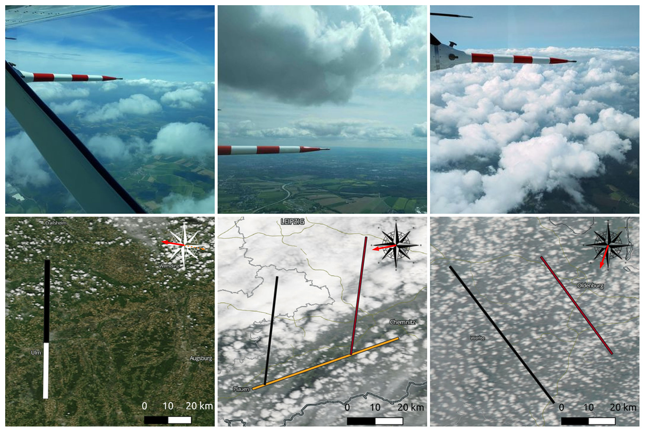
Figure 1Photographs (upper row) and Modis satellite images from NASA Worldview Snapshots (lower row) of the cumulus fields during the flights on 24 May 2019 (left), where white is the cloud-free area and black the cloudy area, 27 May 2019 (middle), where the west track is indicated in black, the east track in red, and the southern track in yellow, and 4 June 2019 (right), where the west track is indicated in black and east track in red. In each satellite picture, the horizontal black and white bar indicates a total distance of 20 km and the mean wind direction during the flight is drawn in the windrose.
During the 2–2.5 h flights, the two aeroplanes flew back and forth across the same pre-defined tracks. Because the two planes have different cruising speed (the Cessna about 70 m s−1, the Falcon about 200 m s−1), the pre-defined tracks ensure overlap in space and time to the degree possible. Flight legs were mostly flown cross wind and ranged from 50 to 100 km in length to ensure sufficient low-frequency wind variability. During some of the flights the tracks were moved or shortened with respect to the original plan to ensure cumulus clouds were captured. All flown tracks are shown in Fig. 1. The terrain below was mostly used for agriculture with low crops, occasionally encountering patches of trees or villages. On the first two flights a hilly topography was present, whereas the last flight was above flat land.
Turbulence measurements using an in situ (3D) turbulence probe aboard the DLR Cessna Grand Caravan were taken at 100 Hz along the track at four different altitudes: within the mixed-layer, near cloud base, within the cloud layer, and through the tops of only the thickest clouds. Employing the downward staring DWLs at a measurement rate of 40 s, the DLR Falcon remained at around 11 km altitude throughout the flight. The instruments are described next.
2.1.1 In situ turbulence probe
The DLR Cessna Grand Caravan was equipped with (i) a meteorological sensor package (METPOD) that measures temperature, humidity, pressure, and wind, and (ii) the IGI systems' AEROcontrol system, which combines measurements of a Differential Global Positioning System (DGPS) with a high-accuracy inertial reference system. Calibration of the devices before the flight and applying corrections afterwards results in a horizontal wind measurement uncertainty of 0.3 and 0.2 m s−1 for the vertical wind component. Further details on the instrument specifics, calibration, correction procedure, and uncertainties can be found in Mallaun et al. (2015).
The high-frequency 100 Hz wind measurements, taken with a boom-mounted Rosemount model 858 AJ air velocity probe, are used for flux calculations. The aircraft movements are corrected using IGI. A linear fit is subtracted from the data before flux calculations. All scales from 10−2 Hz are included in this calculation, unless stated otherwise.
2.1.2 Energy spectra
To check the quality of the measurements, we calculated the power spectral density (based on the fast Fourier transform), after subtracting a linear trend from the data. The Welch method was used with a Hann window with 1000 samples and 50 % overlap to reduce noise in the spectrum. The spectra of the streamwise, cross, and vertical wind components at four heights are displayed in Fig. 2 for the western track on 4 June. Note that the streamwise and cross wind do not change much from zonal and meridional winds. The legs flown in the sub-cloud layer and in the cloud layer contain more energy than the legs flown near the cloud base and cloud top. Comparing the three wind components, turbulence appears to have anisotropic behaviour: from 0.01 to 1 Hz, w contains similar (or in the sub-cloud layer more) energy than u and v. Between 1 and 10 Hz, the streamwise component has the most energy, and w the least. The characteristic slope of the inertial sub-range (dashed line) is seen from ∼ 0.2 to 15 Hz (equivalent to a spatial resolution of 350 m down to 5 m, assuming a typical cruising speed of 65–75 m s−1). From 15 Hz onward, the dampening of the fluctuations in the tube becomes visible and the signal falls of faster, except for one peak at 30 Hz, which is attributed to propeller effects (Mallaun et al., 2015). For calculations of the (eddy-covariance) fluxes and variances, we apply a high-pass filtering after linear detrending, removing the contributions by eddies with a horizontal length scale larger than 7 km (having a frequency lower than 0.01 Hz), a method that is also followed by Brilouet et al. (2021). Filtering out these frequencies will lead to an error because we lose information; however, the random error that is generated by the finite sample size will be reduced (Lenschow et al., 1994).
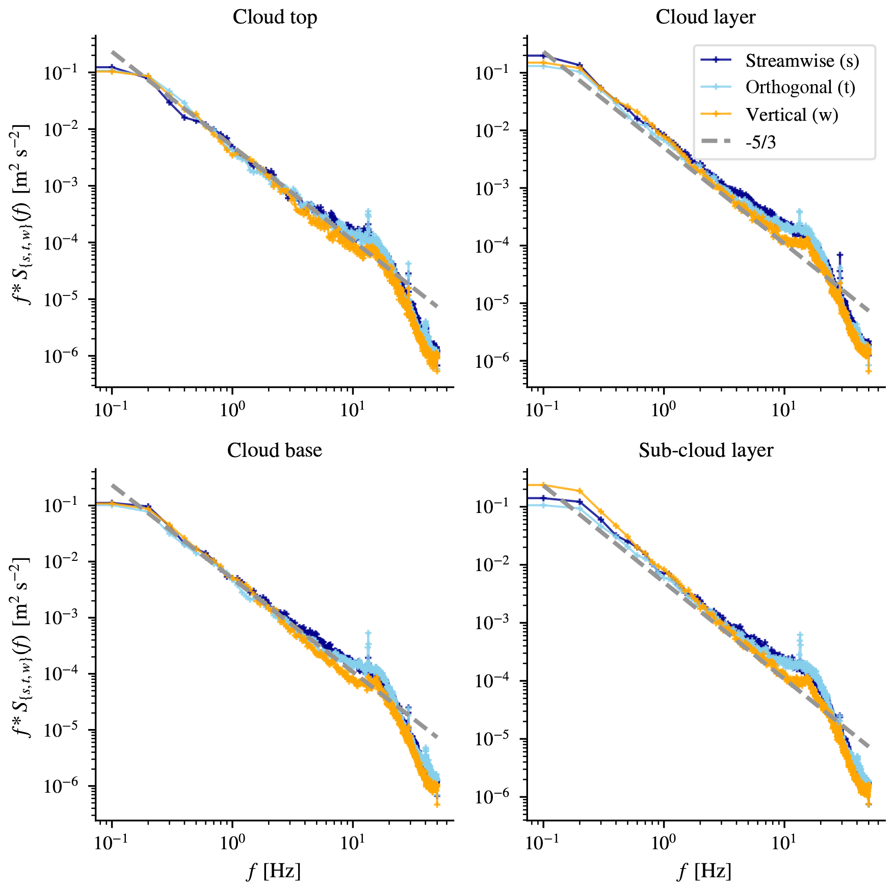
Figure 2Power spectrum of the streamwise, orthogonal, and vertical wind components for the western legs flown on 4 June 2019. Each altitude is shown in an individual panel. The dashed line represents the slope corresponding to the inertial sub-range. The Welch method with a Hann window of 1000 samples and 50 % overlap has been applied to reduce noise.
2.1.3 Eddy-covariance fluxes
The time series are partitioned in leg-averaged values and fluctuating parts ϕ′ by subtracting a linear trend from the time series and applying a high-pass filter, a method that has also been applied by Brilouet et al. (2021). Doing so removes the influence of larger scales having frequencies lower than the cut-off frequency and will lead to a loss of information (Lenschow et al., 1994). Fluxes and variances are then calculated by multiplying and averaging the fluctuations of w and ϕ over a specific time window, known as the “eddy-covariance method”. For instance, the leg average flux of ϕ is given by
The smallest resolved frequency depends on the length of the leg, i.e. on the number of samples N: , in which fs is the sampling rate in Hz. Flying at a cruising speed of ∼ 65–75 m s−1 at a constant height, and with constant ground speed, it is reasonable to assume that a static turbulent field is sampled. However, the statistical representation of the low frequencies is poor and therefore needs cautious interpretation.
2.1.4 Airborne Doppler wind lidar
DWLs are the international standard for wind measurements and have been used for, among other things, (1) data assimilation experiments (e.g. Horányi et al., 2015; Pu et al., 2017; George et al., 2021), (2) to study for instance turbulence, gravity waves, orographic effects (e.g. Yuan et al., 2020; Gisinger et al., 2020; Baidar et al., 2020), and (3) to monitor the flow in wind farms (e.g. Käsler et al., 2010; Wagner et al., 2017; Zhan et al., 2020; Schneemann et al., 2021). The coherent detection DWL employed in this study has a wavelength of 2022.54 nm (approximately 2 µm), being eye-safe and operating in the Rayleigh scattering regime. The (vertical) resolution of the wind measurements depends on both the duration of the pulse, also called “pulse width”, and the distance that the signal can travel during the sampling time. The shorter the pulse, the better the spatial resolution, although a reasonable sampling duration is needed to ensure sufficient accuracy of the velocity estimation (Liu et al., 2019). With a pulse width of ∼ 400 ns and an averaging time of 1 s, we have a vertical resolution of 100 m (i.e. along-beam resolution approx. 94 m) (Witschas et al., 2017). Furthermore, the aircraft speed influences the horizontal resolution. Flying with approximately 200 m s−1 and having a sampling frequency of ∼ 40 s, the horizontal resolution (distance travelled between two measurements) is about 8 km. Pulsed lidars have a blind spot of tens to hundreds of metres near the beam source, depending on the pulse duration and range gate width (Liu et al., 2019). Therefore, although flying at 11 km, the first wind velocities are obtained from approximately 7 km altitude down to about 500 m. The DWL employed in this study has previously been compared with dropsonde measurements, in which the systematic error has been found to remain below 0.1 m s−1 and the random error to vary between 0.92 and 1.5 m s−1 (Weissmann et al., 2005; Chouza et al., 2016; Schaefler et al., 2018; Witschas et al., 2020).
The velocity–azimuth display technique (Browning and Wexler, 1968) with an off-nadir angle of 20∘ is used to retrieve all three wind components. The processing algorithm that is applied to retrieve the wind vectors from one revolution of line-of-sight measurements is described in Witschas et al. (2017).
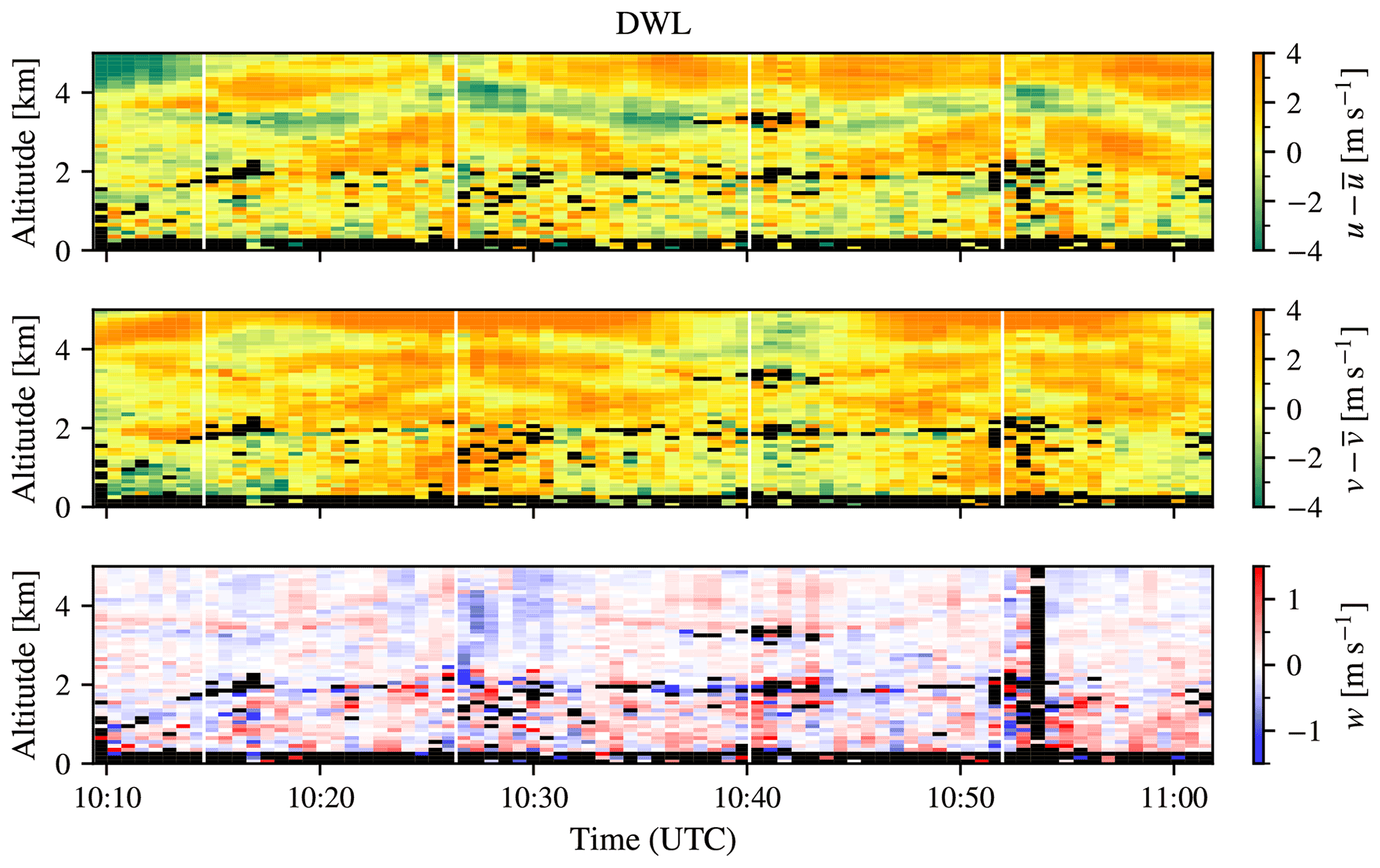
Figure 3Anomalies of zonal (u), meridional (v), and vertical (w) wind measurements from the DWL, zoomed in on the lowest 5 km. Measurements taken on 4 June 2019. Missing values are indicated in black and often correspond to clouds (1–2 km altitude). White vertical lines indicate turning points at the ends of each the track.
Figure 3 shows an example of the wind anomalies (i.e. the wind measurements of which the average wind during the measurement flight is subtracted) on 4 June 2019. The turning points indicating reverse heading on the same leg are indicated with white vertical lines, revealing similar but mirrored wind structures on subsequent legs. On this particular flight, the track was moved further to the east around 11:40 UTC, where different structures are visible. Data gaps, which can be associated with clouds, are indicated in black.
The top of the boundary layer that is at around 2 km altitude is clearly visible in the w fluctuations, with larger fluctuations below, and smaller above. The top of the boundary layer is marked by predominantly blue colours, indicating negative velocities produced by overshooting thermals that become negatively buoyant. Within the boundary layer, updrafts generate the largest fluctuations, while a few downdrafts extending to the surface are also evident. It appears that the DWL can at least to some extent observe the coherent convective features that are responsible for mass transport of scalars and momentum.
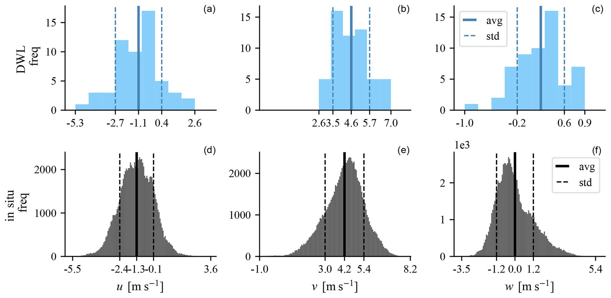
Figure 4Distribution of u, v, and w wind in the sub-cloud layer of the western track at 617 m altitude on 4 June 2019, as measured by the Doppler wind lidar (DWL; a–c, blue) and the in situ turbulence probe (d–f, black). The DWL range bin closest to the in situ flight height was used.
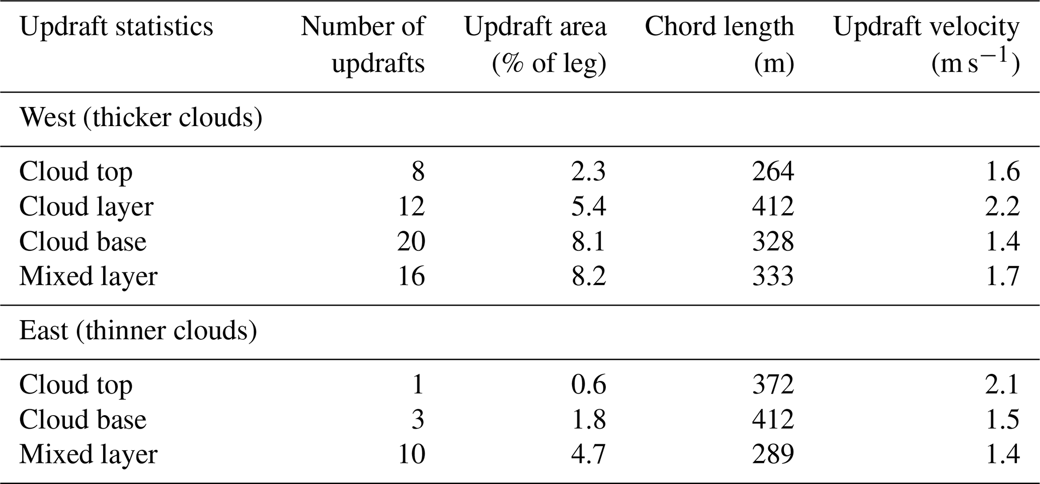
Table 1Number of updrafts, relative updraft area, average updraft size, and average updraft speed for the legs flown on 4 June 2019.
For one of the legs on 4 June, the histograms of the sub-cloud layer u, v, and w wind are compared in Fig. 4. Mean horizontal wind measurements over this leg are comparable for the DWL and in situ measurements. Despite its much coarser resolution and its missing v winds < 2.5 m s−1, the wind variance observed by the DWL is only slightly smaller (0.1 m s−1 less than in the in situ measurements). This gives us confidence that the DWL can provide complementary information of the (horizontal) wind profile at heights where in situ measurements are absent. It also tells us that horizontal wind fluctuations are largely set by scales of 8 km or larger and that cloud convection scales of 1–2 km are less important. On the other hand, the vertical wind shows much less variation than the in situ measurements. This is explained by the much larger area that is measured by the DWL: it can only see the average vertical velocity in this area, which on average is much lower than the vertical velocity of vertical transient small eddies than can be better captured by the in situ measurements.
2.2 Updraft detection algorithm
Using conditional sampling we identify updrafts, following the method described and tested by Lenschow and Stephens (1980). We conditionally sample on updrafts ( & w>0) that are wider than 100 m, and that have an excess in absolute humidity . This method is more robust than using virtual temperature or buoyancy, and can be applied both in the sub-cloud and cloud layer.
Table 1 shows the updraft statistics of the legs flown on 4 June 2019. It lists the number of updrafts, the relative length of the leg that they occupy, the average horizontal size, and the average updraft velocity. We find that the fraction of the leg that is covered by updrafts (updraft area) decreases with height, although the average updraft chord length (the length of the updraft slice that we passed through) peaks at cloud base for the thinner clouds on the eastern track on 4 June as well for the clouds on 24 May 2019 (not shown). On 24 May, we find more and stronger updrafts in the cloud-topped mixed layer than under clear skies, whereas the updraft chord length is comparable. This is in agreement with the findings of, e.g. Nicholls and LeMone (1980), who found stronger sub-cloud and lower cloud-layer vertical velocity standard deviation in more cloudy conditions. The largest average updraft velocity is found at the cloud base, suggesting that the stronger mixed layer updrafts reach the lifted condensation level and benefit from the energy released at condensation. On 4 June, the fastest average updraft speeds are found in the cloud layer in the case of thicker clouds. With the thinner clouds the fastest updraft speed is found at the cloud top, although we must be careful as this includes only one sample.
Although the 3 flight days all captured a shallow cloud regime, they differed substantially in their wind characteristics (wind speed, wind shear, and directional shear), providing a set of diverse case studies, whose wind and thermodynamic profiles are described next. For the wind, an entire profile of the mean and variance is shown from the DWL, with the in situ measurements denoted on top (Fig. 5). Except for the wind direction on 24 May, which varied greatly in the sub-cloud layer, the mean DWL and in situ winds compare very well.
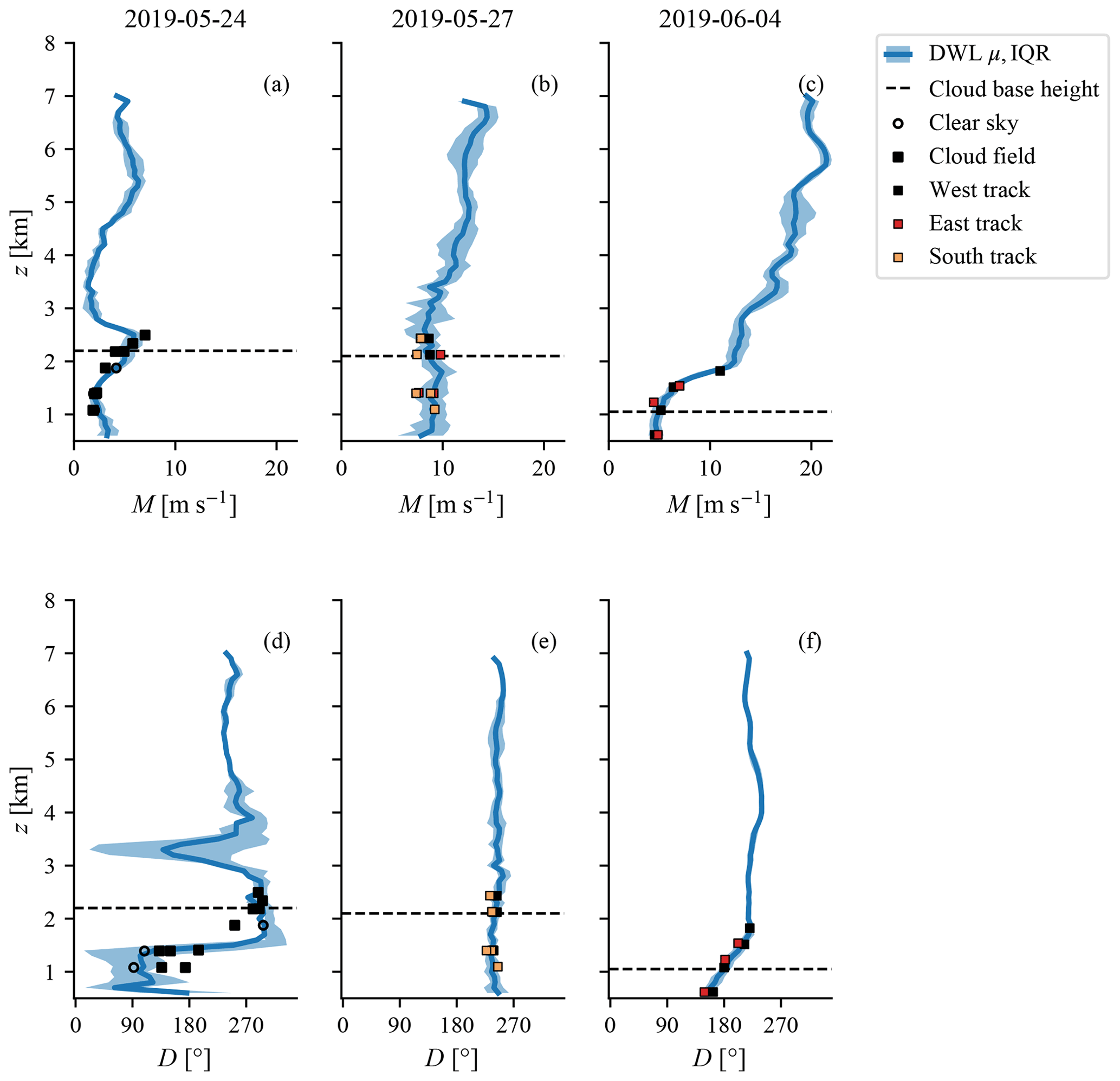
Figure 5Average wind speed and wind direction profiles for each flight date. Average DWL profile indicated in blue, shading indicates the range between the first and third quartile. Average in situ measurement indicated with squares (squares indicate measurements below and in cloud fields) and circles (cloud-free areas). Cloud base height (cbh) was estimated during the flight and is indicated with a horizontal dashed line.
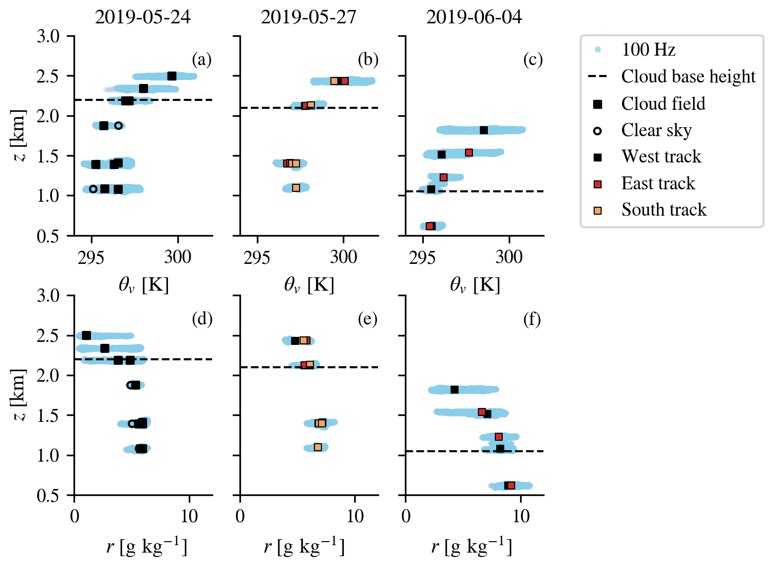
Figure 6Virtual temperature and mixing ratio during the 3 flight days. On the first flight there were three legs that were partly below clear sky and partly below cloudy sky. They have been separated and are represented by open circles and closed squares, respectively. The other two cases had multiple tracks that are indicated with different colours. The raw 100 Hz data are indicated in light blue. Cloud base is indicated by the horizontal dashed line.
The first flight (24 May) took place after a number of overcast days and heavy rain. Southern Germany was under the influence of a broad area of high pressure west of Europe and over the North Atlantic, and the conditions were very stable with hardly any clouds in southern Germany. The northern part of the leg was flown over the Swabian Alps, where numerous gliders were making use of the thermal structures that typically develop here, and shallow cumulus with cloud bases near 2 km (horizontal dashed lines) and tops near 2.5 km developed. These were the focus of our measurements. Winds were weak and reasonably well mixed up to 1400 m, topped by a layer with strong wind turning near 1.5 km (some 500 m below cloud base), and wind speed increased up to 2500 m in a layer extending through cloud base (Fig. 5). By contrast, temperature and humidity were very well mixed vertically. The atmosphere was relatively dry, with a pronounced inversion in temperature and moisture starting near 2.2 km (Fig. 6), as well as a typical region of negative buoyancy below cloud base (Fig. 6) that was not captured in the other two flights.
Considerably stronger wind speeds, but far less wind shear, were present during the second flight (27 May) when we sampled air masses ahead of a cold front located SW-NE across eastern Germany (Figs. 1b, 5b, e). The air masses were somewhat warmer and moister, but with a thermodynamic structure and a cloud base similar to that of the first flight (Fig. 6). Besides shallow convection, there was abundant mid- and upper-level cloud, which we encountered at the end of the first flight leg towards the north. Later, the front seemed to break up and skies were clearer, especially towards the southeast. Eventually, also in the southeastern area of our operations, shallow cumulus made way for stratocumulus layers, with only rare sights of clear sky and sunshine.
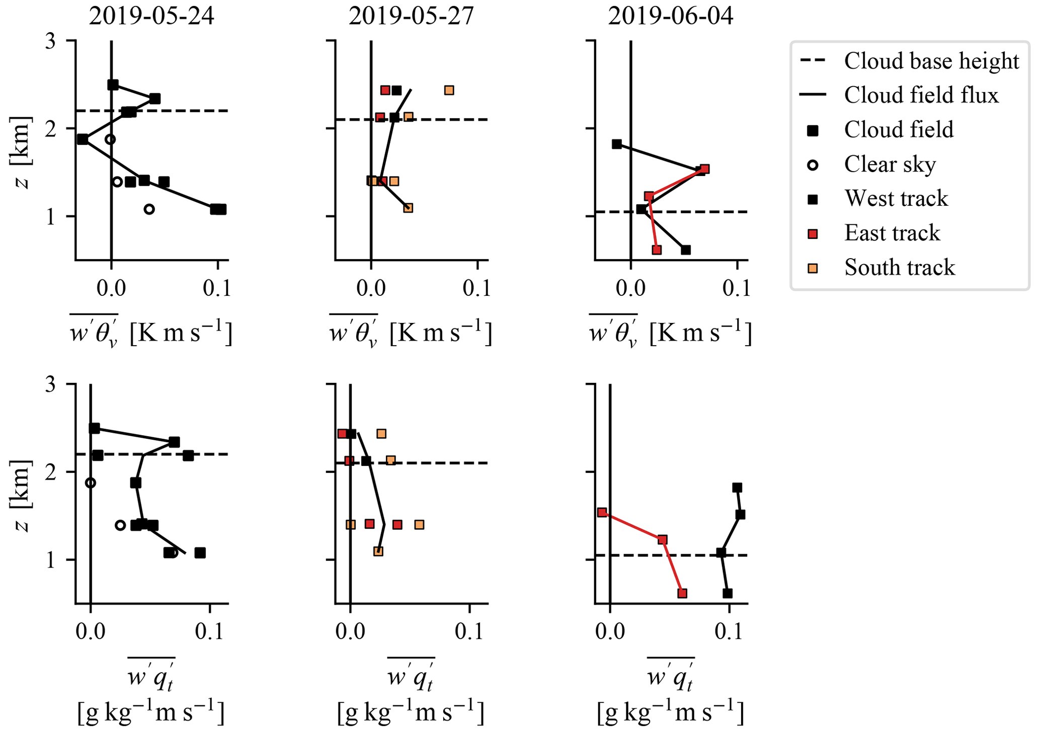
Figure 7Profiles of buoyancy and the moisture flux for the 3 flight days. On the first flight there were three legs that were partly below clear sky and partly below cloudy sky. They have been separated and are represented by open circles and closed squares, respectively. The other two cases had multiple tracks that are indicated with different colours. The average flux below cloudy skies is indicated by a solid line, of which two are present on the last flight day to show the difference between the western and eastern track. Cloud base is indicated by the horizontal dashed line.
During the third flight (4 June), we measured an extended field of shallow cumulus clouds that developed behind a cold front over northwestern Germany in air masses that were considerably colder and moister (Fig. 6c, f), with much lower cloud bases near 1000 (western N-S leg) and 1200 m (eastern N-S leg) and very diverse cloud top heights (see Fig. 1c), with maximum tops near 2 km. The cloud field was organized in patches of alternating cloudy and cloud-free air masses. As the clouds got deeper towards the northern parts of the leg, the relative sizes of the patches increased. The difference in the inversion strength of the temperature profile is clearly visible between the western and eastern leg (Fig. 6c), as well as a large difference in moisture flux (Fig. 7). Near-surface winds were weak and from the south, with strong shear and a turning from southeasterly to southwesterly winds right around cloud base (Fig. 5c, f).
Based on the wind profiles, the three flights could be classified as having weak wind and strong shear either in the sub-cloud layer (Flight 1) or in the cloud layer (Flight 3), and having strong wind but little shear (Flight 2). In the next section, we explore the associated turbulent statistics of these flights and evaluate whether the derived momentum flux profiles are in line with our expectations, e.g. that momentum fluxes throughout the mixed layer and cloud layer increase with wind shear as predicted by K theory.
4.1 Sub-cloud and cloud layer profiles
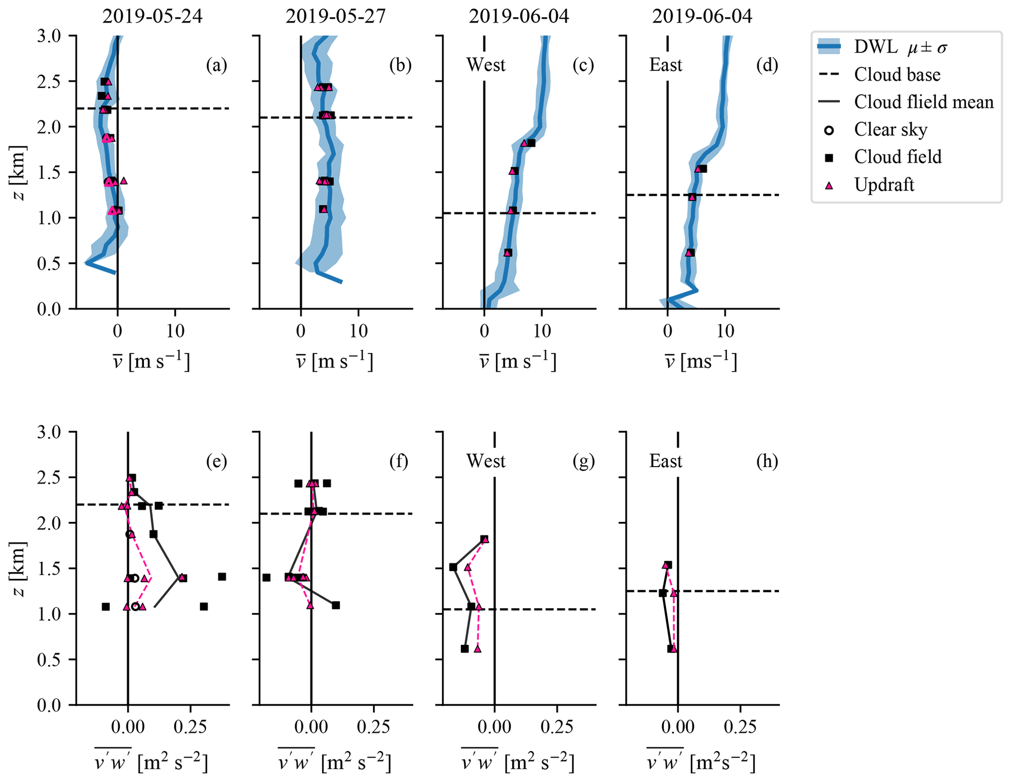
In Figs. 8 and 9 we consider the profiles of wind and momentum flux for the vector wind components u and v separately. As in Fig. 5, the wind speed is shown for both the DWL (in blue) and the in situ turbulence probe at the flight levels (circles, squares). A guideline for the flux profiles in cloudy conditions is indicated in solid black lines, which are linearly interpolated between leg-averaged values at the different flight levels (and are sometimes averaged over multiple legs at the same level).
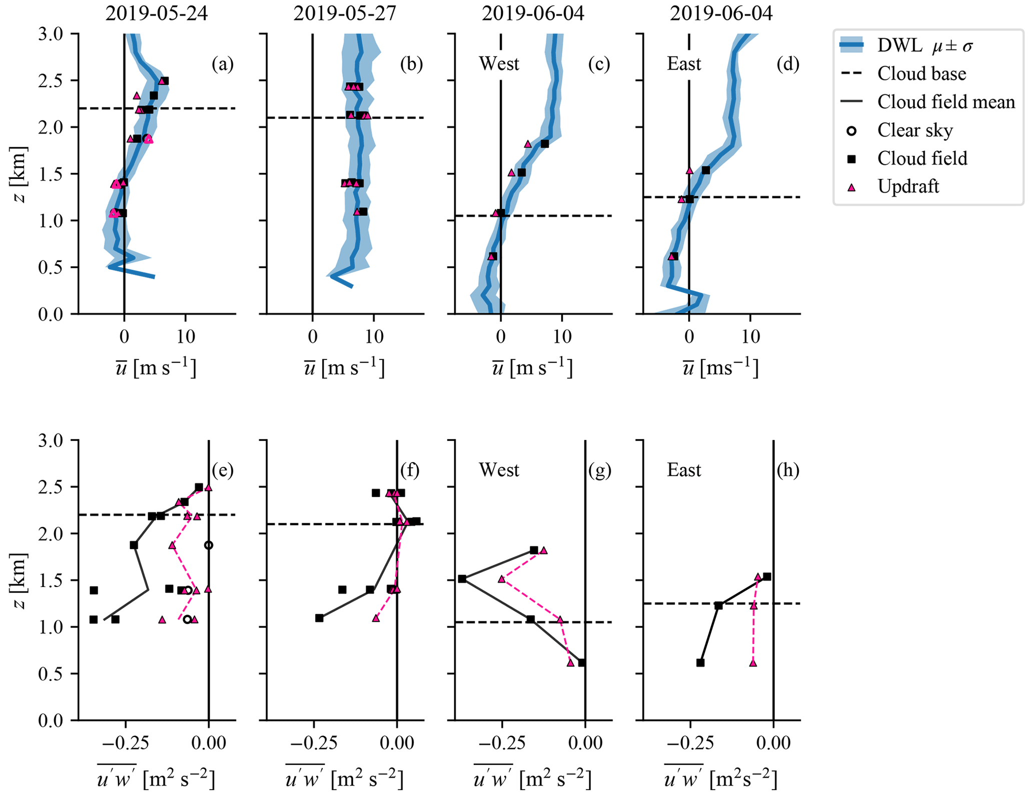
Figure 8Average u (a–d) and (e–h) profiles for each flight date. The u axis is positive eastward. To obtain these profiles, we applied the same averaging procedure as in Fig. 5 and the eddy-covariance method as described in Sect. 2.1.3. On 24 May 2019 (a, e), the clear-sky measurements are indicated with open circles, whereas measurements in cloud fields are indicated with filled squares. Pink triangles represent the wind speed within updrafts (upper panels) and updraft contribution to the total flux (lower panels).
When fluxes are dominated by small-scale turbulent diffusion, it may be modelled (parameterized) by using so-called flux–gradient relationships, also known as “K diffusion”. We find that most of the fluxes and their relationship with the wind gradient lead to a K value that is in line with down-gradient diffusion, acting to reduce the wind gradient.
On 24 May, ignoring the strong gradients in u below ∼ 700 m, . This implies that air parcels that are displaced upward () generally have a negative u perturbation compared with their environment (), acting to remove the wind gradient, in line with K theory. This holds generally for all flight days. Negative u perturbations are in particular evident from the actual wind in air masses sampled within updrafts, which tend to be several m s−1 slower (pink triangles in Figs. 8 and 9). Similarly, the meridional momentum fluxes are also down-gradient; for example, the gradient above 1 km on 24 May, corresponding to a positive meridional momentum flux (), and on 4 June, corresponding to .
The profiles of reveal that larger fluxes are measured on 24 May than on 27 May, in line with the stronger shear present in u and (to a lesser extent) in v. Fluxes typically decrease towards the boundary layer height (cloud top or mixed-layer top in the case of clear sky) as the variance of vertical velocity decreases towards the top of the boundary layer (Fig. 10).
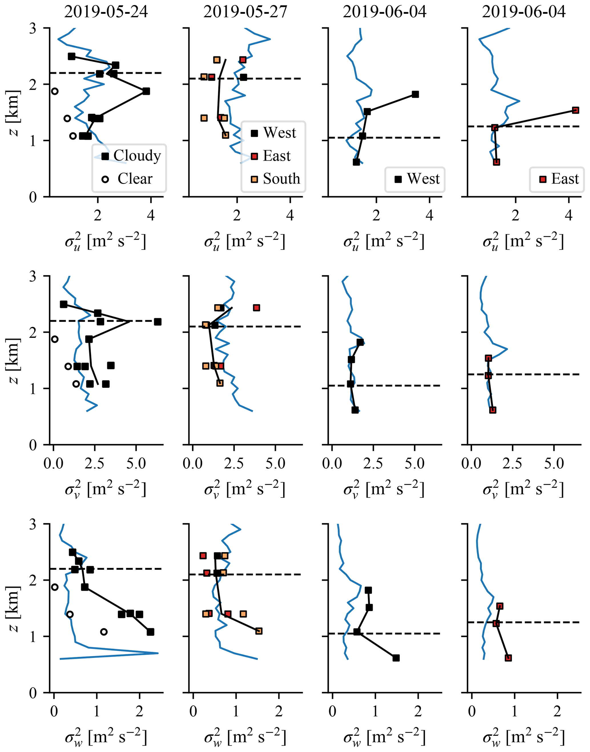
Evidently, on 24 May the momentum fluxes throughout the mixed layer increased considerably from the first transect of the flight, which captured a dry convective boundary layer (open circles), to the second transect, which is when cumulus clouds developed on top of the mixed layer (filled squares), although both transects have comparable u,v profiles (Figs. 8, 9). The larger fluxes reflect the presence of stronger turbulent eddies. Especially just below and at cloud base, much larger variances are present in u and v, and throughout the mixed layer in w (Fig. 10).
While on 24 May, on 27 May, and the eastern leg on 4 June the fluxes decreased towards cloud base, with little flux remaining in the cloud layer, the western leg on 4 June shows an increase in momentum fluxes with height (in particular but also ). Whereas the flux in the mixed layer below clouds is almost negligible, one of the largest fluxes was measured in the cloud layer ( m2 s−2). Clouds on this western leg had a lower base (just above 1 km) and higher cloud tops (up to 2 km) and thus were thicker than the clouds that were encountered on the eastern track. The thicker clouds have not only a larger momentum transport in the cloud layer, but also a much larger (percentage) contribution of the updraft to the total flux than any of the other measurements (Fig. 6). The fraction of the leg that was occupied by updrafts was also significantly larger than in all other cases. The deeper clouds may have been accompanied by wider updrafts with better protected cores that may be responsible for carrying larger fluxes.
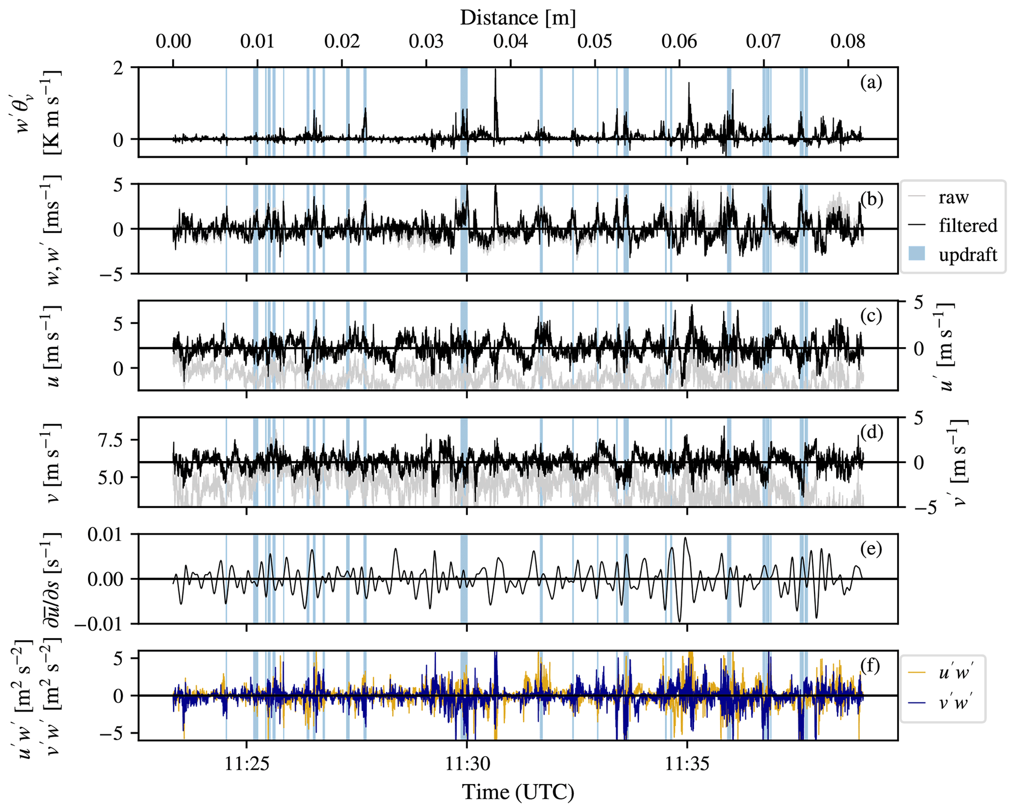
Figure 11Raw (unfiltered) and fluctuating (filtered: linear detrended, high-pass filter cut-off 0.01 Hz) time series of (a) buoyancy flux, (b) vertical velocity, (c) zonal wind, (d) meridional wind, (e) convergence and divergence of the wind speed in the streamwise direction calculated using a low-pass filter that considers all scales larger than 700 m (fc<0.1 Hz), and (f) momentum fluxes measured on 4 June 2019 at 600 m, in the middle of the mixed layer of the western leg. Updrafts are indicated with light-blue shading.
Figure 11 shows a time series of turbulence measured at 600 m in the mixed layer on the western track on 4 June. The unfiltered turbulence statistics are shown in grey, while black shows the linearly detrended and high-pass filtered (f>0.01 Hz) statistics. Cloudy updrafts can have vertical speeds up to 5 m s−1, in both altitudes. Evidently, large buoyancy fluxes (, top row) are associated with large momentum fluxes (bottom row), which reveals the importance of convection in generating a large momentum flux. Sometimes, for instance at 11:33 UTC, the convergence (Fig. 11e) is closely tied to convection. Typically, updrafts carry wind speeds that are much slower (up to 5 m s−1 for cloudy updrafts) than the environment. Looking carefully, one can see that u′ and w′ peak at different times and that u′ has a different sign in various updrafts. This could explain a much lower momentum flux. We discuss this further in the next few sections, where we explore the fluxes sampled on (cloudy) updrafts, as well as how eddies of different scales contribute to the fluxes.
4.2 Scale contributions to flux
Observations in the surface layer, for instance during the Kansas experiment, show that the cospectra of the flux follow a fixed slope, with the large scales being more significant (Kaimal et al., 1972). However, throughout the boundary layer, large-eddy simulations of various cases indicate that the momentum flux carried by small-scale shear-driven turbulent eddies (with a size smaller than ∼ 200 m) can contribute more than 50 % of momentum fluxes. Small-scale turbulence may also transport momentum in an opposite direction than larger more coherent eddy structures (Zhu, 2015). This is particularly true for the lower mixed layer and near cloud tops. However, in shallow cumulus cases, especially from the middle of the mixed layer (sub-cloud layer) to the middle of the cloud layer, the net momentum fluxes are almost entirely carried by eddies with scales greater than 400 m (Zhu, 2015).

Figure 12Scale contributions to the momentum flux (upper panels) and (lower panels) for different heights in the atmosphere. The bars in each panel represent the flux contribution, in which the left-most bar only includes small scales (frequencies exceeding 0.2 Hz) and the right-most bar includes all scales that are represented in the measurements limited to 7 km (with a cut-off frequency of 0.01 Hz, excluding lower frequencies). Filter scales are 0.20, 0.15, 0.10, 0.05, 0.025, and 0.001 Hz that, when assuming a cruising speed of 70 m s−1, correspond to length scales of 350, 467, 700, 1400, 2800, and 7000 m, respectively. The black bars represent the western leg with thicker clouds, the red bars represent the eastern leg with thinner clouds.
In Fig. 12, the total (net) momentum flux is shown for the legs in the sub-cloud layer, near the cloud base, within the cloud layer, and near the cloud top for 4 June. The momentum flux at different scales is calculated using a high-pass filter that removes larger scales with increasing cut-off frequency. The flux all the way to the right is, for instance carried by eddies up to a scale of ∼ 7 km, corresponding to a cut-off frequency of 0.01 Hz. When the flux magnitude increases rapidly from left to right, it implies that larger-scale eddies contribute more to the momentum flux than smaller scales. If considerable flux is already at smaller scales (higher cut-off frequencies), as is the case in the zonal flux at cloud top in the eastern leg, the smaller eddies play a more important role.
The results suggest that momentum fluxes carried by eddies of different scales can counteract to reduce the overall flux. The relatively small flux (in the profiles, Figs. 8, 9), for instance in in the mixed layer on the western leg with thicker clouds is produced by a positive carried by scales larger than 2.8 km up to maximally 7 km (fc=0.025–0.01 Hz), which almost compensates for the negative flux carried by turbulence on scales less than 2.8 km (fc=0.025 Hz).
The same is true for near cloud top in the eastern leg with thinner clouds, and to a lesser extent in the flux of in that leg within the mixed layer and near cloud tops. In the leg with thick clouds, the change in sign of the flux takes place already between 0.7 and 2.8 km. In other words, the profiles deviate from a profile where fluxes linearly decrease with height when scales beyond 1–2 km (cloud scale) play an important role.
Having less shear, for instance on 27 May, the fluxes are much smaller in general (Figs. 8 and 9). There, smaller scales do not matter much and the flux is solely generated by the largest scales (not shown).
In this paper we aimed to investigate the variability in wind profiles and momentum fluxes under convective conditions, motivated by a lack of knowledge on the nature of the momentum flux profile in cloud-topped boundary layers. As in seminal marine cumulus field studies, we used traditional in situ turbulence measurements on board a Cessna aircraft that flew 50–100 km tracks at different legs below and within the cloud layer. These measurements were complemented with downward profiling Doppler wind lidar (DWL) measurements onboard a Falcon aircraft that flew the same track at higher altitudes. DWLs are not typically employed in field studies of convection and clouds, but can help elucidate flows on mesoscales that accompany (organized) convection.
We carried out a limited number of flights in different wind and convective conditions. The first day had calm winds, but strong directional shear with areas of clear sky as well as areas with convective cumulus humilis of maximum 500 m extend. The two other days displayed pre-frontal convection with weak shear and post-frontal convection with strong shear. On both days convection was deeper than in the first case and was embedded in flows with strong winds.
First, we aimed to answer how the wind profiles and variance in the in situ and DWL measurements compare. Both the mean horizontal wind and the variance of horizontal wind at given heights compared well despite the much larger horizontal sampling scale of the DWL (7 km vs 70 m). Wind fluctuations on scales larger than turbulence and (cloudy) updrafts (on meso-gamma scales from 2 to 20 km) were found to be up to ±5 m s−1. This emphasizes that flight legs need to be sufficiently long to capture mesoscale fluctuations in the mean wind (and its variance).
The profiles of wind derived from the few sampling legs of the Cessna compared reasonably well with the DWL profiles, in other words, the wind profile did not evolve significantly during the course of the flight as the Cessna transitioned from one leg altitude to another. The DWL also revealed the location of up- and downdrafts, such as negative vertical velocities at the top of the boundary layer where thermal plumes encounter a warmer environment and become negatively buoyant.
Second, we asked whether the measured momentum flux profiles in the sub-cloud layer and in the cloud layer are in line with our expectations, as well as to what extent we can explain them from convective updrafts alone. On the same flight day and even on the same track, substantial differences in the momentum flux could be seen associated with regions of convection. Most of the momentum flux profiles revealed down-gradient momentum transport that was generally strongest within the mixed layer and decreasing towards cloud tops, but counter-gradient transport was also observed on the third flight day with post-frontal convection and strong shear, on which distinct alternating patches of clear sky and sheared clouds of about 1 km deep were seen. Different flight segments, even on that same flight day, had a very different momentum flux profile that was not explained by turbulent transport across the local vertical gradient in the wind.
Although momentum fluxes generally increased in areas with (cloudy) updrafts, the contribution of the updraft to the total momentum flux was typically (only) one-third to two-thirds, which is comparatively small considering the contribution of the updraft to the buoyancy flux (pending). Horizontal momentum perturbations carried by updrafts below and within clouds were clearly distinguishable on all flights, but especially large on the third flight (up to almost 5 m s−1 in the cloud layer).
Finally, we asked which scales contribute significantly to wind variance and the momentum flux. We found that scales beyond 1 km contribute significantly to the momentum flux and there is clear evidence for compensating flux contributions from different scales. In the post-frontal convection day, cancellation of fluxes of different signs may have explained a differing momentum flux profile with relatively small fluxes in the well-mixed sub-cloud layer (compared with the fluxes in the cloud layer).
The limited number of flights do not allow us to draw a general conclusion across a wide range of convective states. Nevertheless, they highlight that momentum flux profiles and their variability require understanding of motions across a range of scales, with non-negligible contributions of the clear-sky fluxes and of mesoscales that may be coupled with the convection. Wind lidars can help elucidate the flows on larger than cloud scales and should be used more deliberately in studies of clouds and their spatial organization.
Data are made publicly available on the 4TU Data Repository (https://doi.org/10.4121/18614102.v1, Mallaun et al., 2022).
AMK and LN conceptualized the study, and AMK was responsible for the data analysis and writing of the manuscript. CM was responsible for the technical preparation of the flight data and his experience aided significantly in the decision on an approach for eddy covariance estimation. LN was also involved in the supervision. All authors provided critical comments on the quality of the work. CL was the principal investigator (PI) of the parallel Aeolus validation campaign (AVATARE) and of the A2D deployed in the DLR Falcon aircraft, which was also used for the CloudBrake flights. Additionally, he supported the campaign preparation and flight planning. BW was responsible for the 2 µm DWL measurements, operated the system during CloudBrake flights, and performed part of the data analysis. Furthermore, he contributed to the scientific interpretation of the DWL data as discussed in this paper.
The contact author has declared that neither they nor their co-authors have any competing interests.
Publisher’s note: Copernicus Publications remains neutral with regard to jurisdictional claims in published maps and institutional affiliations.
This project has received funding from the European Research Council (ERC) under the European Union's Horizon 2020 research and innovation programme (Starting Grant, grant no. 714918). The Falcon lidar instrumentation was funded for the Aeolus validation by the European Space Agency (grant no. 4000128136/19/NL/IA). We thank our ESA colleague Thorsten Fehr (Aeolus scientific campaign coordinator) for his support of the AVATARE campaign as well as Stephan Rahm (DLR) for the rapid and sophisticated pre-processing of the 2 µm DWL data. The authors are also grateful to the DLR Flight Experiments department for the realization of the two airborne campaigns in parallel. Furthermore, we want to thank Margaret LeMone and Chris Fairall for taking the time to review this paper. Their constructive comments led to improvements in this paper.
This research has been supported by the European Research Council (ERC) under the European Union's Horizon 2020 research and innovation programme (grant no. 714918).
This paper was edited by Holger Tost and reviewed by Margaret LeMone and Christopher Fairall.
Baidar, S., Bonin, T., Choukulkar, A., Brewer, A., and Hardesty, M.: Observation of the urban wind island effect, EPJ Web Conf., 237, 06009, https://doi.org/10.1051/epjconf/202023706009, 2020. a
Bakhshi, R. and Sandborn, P.: Maximizing the returns of LIDAR systems in wind farms for yaw error correction applications, Wind Energy, 23, 1408–1421, https://doi.org/10.1002/we.2493, 2020. a
Banta, R., Pichugina, Y., Kelley, N., Hardesty, R., and Brewer, W.: Wind Energy Meteorology: Insight into Wind Properties in the Turbine-Rotor Layer of the Atmosphere from High-Resolution Doppler Lidar, B. Am. Meteorol. Soc., 94, 883–902, https://doi.org/10.1175/BAMS-D-11-00057.1, 2013. a
Brilouet, P.-E., Lothon, M., Etienne, J.-C., Richard, P., Bony, S., Lernoult, J., Bellec, H., Vergez, G., Perrin, T., Delanoë, J., Jiang, T., Pouvesle, F., Lainard, C., Cluzeau, M., Guiraud, L., Medina, P., and Charoy, T.: The EUREC4A turbulence dataset derived from the SAFIRE ATR 42 aircraft, Earth Syst. Sci. Data, 13, 3379–3398, https://doi.org/10.5194/essd-13-3379-2021, 2021. a, b
Browning, K. A. and Wexler, R.: The Determination of Kinematic Properties of a Wind Field Using Doppler Radar, Journal of Applied Meteorology and Climatology, J. Appl. Meteorol. Clim., 1, 105–113, https://doi.org/10.1175/1520-0450(1968)007<0105:TDOKPO>2.0.CO;2, 1968. a
Chouza, F., Reitebuch, O., Jähn, M., Rahm, S., and Weinzierl, B.: Vertical wind retrieved by airborne lidar and analysis of island induced gravity waves in combination with numerical models and in situ particle measurements, Atmos. Chem. Phys., 16, 4675–4692, https://doi.org/10.5194/acp-16-4675-2016, 2016. a
Dixit, V., Nuijens, L., and Helfer, K.: Counter-gradient momentum transport through subtropical shallow convection in ICON-LEM simulations, J. Adv. Model. Earth Syst., 13, e2020MS002352, https://doi.org/10.1029/2020MS002352, 2021. a
George, G., Halloran, G., Kumar, S., Indira Rani, S., Bushair, M., Jangid, B., George, J., and Maycock, A.: Impact of Aeolus horizontal line of sight wind observations in a global NWP system, Atmos. Res., 261, 105742, https://doi.org/10.1016/j.atmosres.2021.105742, 2021. a
Gisinger, S., Wagner, J., and Witschas, B.: Airborne measurements and large-eddy simulations of small-scale gravity waves at the tropopause inversion layer over Scandinavia, Atmos. Chem. Phys., 20, 10091–10109, https://doi.org/10.5194/acp-20-10091-2020, 2020. a
Helfer, K. C. and Nuijens, L.: The Morphology of Simulated Trade-Wind Convection and Cold Pools Under Wind Shear, J. Geophys. Res.-Atmos., 126, e2021JD035148, https://doi.org/10.1029/2021JD035148, 2021. a
Horányi, A., Cardinali, C., Rennie, M., and Isaksen, L.: The assimilation of horizontal line-of-sight wind information into the ECMWF data assimilation and forecasting system. Part I: The assessment of wind impact, Q. J. Roy. Meteor. Soc., 141, 1223–1232, https://doi.org/10.1002/qj.2430, 2015. a
Iungo, G. V. and Porté-Agel, F.: Measurement procedures for characterization of wind turbine wakes with scanning Doppler wind LiDARs, Adv. Sci. Res., 10, 71–75, https://doi.org/10.5194/asr-10-71-2013, 2013. a
Kaimal, J. C., Wyngaard, J. C. J., Izumi, Y., and Coté, O. R.: Spectral characteristics of surface‐layer turbulence, Q. J. Roy. Meteor. Soc., 98, 563–589, 1972. a
Käsler, Y., Rahm, S., Simmet, R., and Kühn, M.: Wake Measurements of a Multi-MW Wind Turbine with Coherent Long-Range Pulsed Doppler Wind Lidar, J. Atmos. Ocean. Tech., 27, 1529–1532, https://doi.org/10.1175/2010JTECHA1483.1, 2010. a
Krishnamurthy, R., Choukulkar, A., Calhoun, R., Fine, J., Oliver, A., and Barr, K.: Coherent Doppler lidar for wind farm characterization, Wind Energy, 16, 189–206, https://doi.org/10.1002/we.539, 2013. a
LeMone, M. and Pennell, W.: The Relationship of Trade Wind Cumulus Distribution to Subcloud Layer Fluxes and Structure, Mon. Weather Rev., 104, 524–539, https://doi.org/10.1175/1520-0493(1976)104<0524:TROTWC>2.0.CO;2, 1976. a
Lenschow, D. and Stephens, P.: The role of thermals in the convective boundary layer, Bound.-Lay. Meteorol., 19, 509–532, https://doi.org/10.1007/BF00122351, 1980. a
Lenschow, D. H., Mann, J., and Kristensen, L.: How Long Is Long Enough When Measuring Fluxes and Other Turbulence Statistics?, J. Atmos. Ocean. Tech., 11, 661–673, https://doi.org/10.1175/1520-0426(1994)011<0661:HLILEW>2.0.CO;2, 1994. a, b
Li, Z., Zuidema, P., and Zhu, P.: Simulated Convective Invigoration Processes at Trade Wind Cumulus Cold Pool Boundaries, J. Atmos. Sci., 71, 2823–2841, https://doi.org/10.1175/JAS-D-13-0184.1, 2014. a
Liu, Z., Barlow, J., Chan, P., Fung, J. C. H., Li, Y., Ren, C., Mak, H. W. L., and Ng, E.: A Review of Progress and Applications of Pulsed Doppler Wind LiDARs, Remote Sens., 11, 2522, https://doi.org/10.3390/rs11212522, 2019. a, b
Lux, O., Lemmerz, C., Weiler, F., Marksteiner, U., Witschas, B., Rahm, S., Geiß, A., and Reitebuch, O.: Intercomparison of wind observations from the European Space Agency's Aeolus satellite mission and the ALADIN Airborne Demonstrator, Atmos. Meas. Tech., 13, 2075–2097, https://doi.org/10.5194/amt-13-2075-2020, 2020. a
Mallaun, C., Giez, A., and Baumann, R.: Calibration of 3-D wind measurements on a single-engine research aircraft, Atmos. Meas. Tech., 8, 3177–3196, https://doi.org/10.5194/amt-8-3177-2015, 2015. a, b
Mallaun, C., Rahm, S., Witschas, B., and Nuijens, L.: CloudBrake wind measurement flights on three cumulus days, 4TU.ResearchData [data set], https://doi.org/10.4121/18614102.v1, 2022. a
Mann, J., Peña, A., Bingöl, F., Wagner, R., and Courtney, M. S.: Lidar Scanning of Momentum Flux in and above the Atmospheric Surface Layer, J. Atmos. Ocean. Tech., 27, 959–976, https://doi.org/10.1175/2010JTECHA1389.1, 2010. a
Nicholls, S. and LeMone, M.: The Fair Weather Boundary Layer in GATE: The Relationship of Subcloud Fluxes and Structure to the Distribution and Enhancement of Cumulus Clouds, J. Atmos. Sci., 37, 2051–2067, https://doi.org/10.1175/1520-0469(1980)037<2051:TFWBLI>2.0.CO;2, 1980. a
Pu, Z., Zhang, L., Zhang, S., Gentry, B., Emmitt, D., Demoz, B., and Atlas, R.: The Impact of Doppler Wind Lidar Measurements on High-Impact Weather Forecasting: Regional OSSE and Data Assimilation Studies, Springer International Publishing, Cham, 259–283, https://doi.org/10.1007/978-3-319-43415-5_12, 2017. a
Saggiorato, B., Nuijens, L., Siebesma, A. P., de Roode, S., Sandu, I., and Papritz, L.: The Influence of Convective Momentum Transport and Vertical Wind Shear on the Evolution of a Cold Air Outbreak, J. Adv. Model. Earth Syst., 12, e2019MS001991, https://doi.org/10.1029/2019MS001991, 2020. a
Schaefler, A., Craig, G., Wernli, H., Arbogast, P., Doyle, J. D., McTaggart-Cowan, R., J., M., G., R., Ament, F., Boettcher, M., Bramberger, M., Cazenave, Q., Cotton, R., Crewell, S., Delanoë, J., Dörnbrack, A., Ehrlich, A., Ewald, F., Fix, A., Grams, C. M., Gray, S. L., Grob, H., Groß, S., Hagen, M., Harvey, B., Hirsch, L., Jacob, M., Kölling, T., Konow, H., Lemmerz, C., Lux, O., Magnusson, L., Mayer, B., Mech, M., Moore, R., Pelon, J., Quinting, J., Rahm, S., Rapp, M., Rautenhaus, M., Reitebuch, O., Reynolds, C. A., Sodemann, H., Spengler, T., Vaughan, G., Wendisch, M., Wirth, M., Witschas, B., Wolf, K., and Zinner, T.: The North Atlantic Waveguide and Downstream Impact Experiment, B. Am. Meteorol. Soc., 99, 1607–1637, https://doi.org/10.1175/BAMS-D-17-0003.1, 2018. a
Schlemmer, L., Bechtold, P., Sandu, I., and Ahlgrimm, M.: Uncertainties related to the representation of momentum transport in shallow convection, J. Adv. Model. Earth Syst., 9, 1269–1291, https://doi.org/10.1002/2017MS000915, 2017. a
Schneemann, J., Theuer, F., Rott, A., Dörenkämper, M., and Kühn, M.: Offshore wind farm global blockage measured with scanning lidar, Wind Energ. Sci., 6, 521–538, https://doi.org/10.5194/wes-6-521-2021, 2021. a
Wagner, J., Dörnbrack, A., Rapp, M., Gisinger, S., Ehard, B., Bramberger, M., Witschas, B., Chouza, F., Rahm, S., Mallaun, C., Baumgarten, G., and Hoor, P.: Observed versus simulated mountain waves over Scandinavia – improvement of vertical winds, energy and momentum fluxes by enhanced model resolution?, Atmos. Chem. Phys., 17, 4031–4052, https://doi.org/10.5194/acp-17-4031-2017, 2017. a
Weissmann, M., Busen, R., Dörnbrack, A., Rahm, S., and Reitebuch, O.: Targeted Observations with an Airborne Wind Lidar, J. Atmos. Ocean. Tech., 22, 1706–1719, https://doi.org/10.1175/JTECH1801.1, 2005. a
Witschas, B., Rahm, S., Dörnbrack, A., Wagner, J., and Rapp, M.: Airborne Wind Lidar Measurements of Vertical and Horizontal Winds for the Investigation of Orographically Induced Gravity Waves, J. Atmos. Ocean. Tech., 34, 1371–1386, https://doi.org/10.1175/JTECH-D-17-0021.1, 2017. a, b
Witschas, B., Lemmerz, C., Geiß, A., Lux, O., Marksteiner, U., Rahm, S., Reitebuch, O., and Weiler, F.: First validation of Aeolus wind observations by airborne Doppler wind lidar measurements, Atmos. Meas. Tech., 13, 2381–2396, https://doi.org/10.5194/amt-13-2381-2020, 2020. a, b
Yuan, J., Xia, H., Wei, T., Wang, L., Yue, B., and Wu, Y.: Identifying cloud, precipitation, windshear, and turbulence by deep analysis of the power spectrum of coherent Doppler wind lidar, Opt. Express, 28, 37406–37418, 2020. a
Zhan, L., Letizia, S., and Iungo, G. V.: LiDAR measurements for an onshore wind farm: Wake variability for different incoming wind speeds and atmospheric stability regimes, Wind Energy, 23, 501–527, https://doi.org/10.1002/we.2430, 2020. a
Zhu, P.: On the Mass-Flux Representation of Vertical Transport in Moist Convection, J. Atmos. Sci., 72, 4445–4468, https://doi.org/10.1175/JAS-D-14-0332.1, 2015. a, b, c
Zuidema, P., Li, Z., Hill, R., Bariteau, L., Rilling, B., Fairall, C., Brewer, W., Albrecht, B., and Hare, J.: On Trade Wind Cumulus Cold Pools, J. Atmos. Sci., 69, 258–280, https://doi.org/10.1175/JAS-D-11-0143.1, 2012. a
The requested paper has a corresponding corrigendum published. Please read the corrigendum first before downloading the article.
Please read the editorial note first before accessing the article.
- Article
(5807 KB) - Full-text XML