the Creative Commons Attribution 4.0 License.
the Creative Commons Attribution 4.0 License.
 | 07 Jun 2022
Evaluating seasonal and regional distribution of snowfall in regional climate model simulations in the Arctic
Annakaisa von Lerber
Mario Mech
Annette Rinke
Damao Zhang
Melanie Lauer
Ana Radovan
Irina Gorodetskaya
Susanne Crewell
In this study, we investigate how the regional climate model HIRHAM5 reproduces the spatial and temporal distribution of Arctic snowfall when compared to CloudSat satellite observations during the examined period of 2007–2010. For this purpose, both approaches, i.e., the assessments of the surface snowfall rate (observation-to-model) and the radar reflectivity factor profiles (model-to-observation), are carried out considering spatial and temporal sampling differences. The HIRHAM5 model, which is constrained in its synoptic representation by nudging to ERA-Interim, represents the snowfall in the Arctic region well in comparison to CloudSat products. The spatial distribution of the snowfall patterns is similar in both identifying the southeastern coast of Greenland and the North Atlantic corridor as regions gaining more than twice as much snowfall as the Arctic average, defined here for latitudes between 66 and 81∘ N. Excellent agreement (difference less than 1 %) in the Arctic-averaged annual snowfall rate between HIRHAM5 and CloudSat is found, whereas ERA-Interim reanalysis shows an underestimation of 45 % and significant deficits in the representation of the snowfall rate distribution. From the spatial analysis, it can be seen that the largest differences in the mean annual snowfall rates are an overestimation near the coastlines of Greenland and other regions with large orographic variations as well as an underestimation in the northern North Atlantic Ocean. To a large extent, the differences can be explained by clutter contamination, blind zone or higher resolution of CloudSat measurements, but clearly HIRHAM5 overestimates the orographic-driven precipitation. The underestimation of HIRHAM5 within the North Atlantic corridor south of Svalbard is likely connected to a poor description of the marine cold air outbreaks which could be identified by separating snowfall into different circulation weather type regimes. By simulating the radar reflectivity factor profiles from HIRHAM5 utilizing the Passive and Active Microwave TRAnsfer (PAMTRA) forward-modeling operator, the contribution of individual hydrometeor types can be assessed. Looking at a latitude band at 72–73∘ N, snow can be identified as the hydrometeor type dominating radar reflectivity factor values across all seasons. The largest differences between the observed and simulated reflectivity factor values are related to the contribution of cloud ice particles, which is underestimated in the model, most likely due to the small sizes of the particles. The model-to-observation approach offers a promising diagnostic when improving cloud schemes, as illustrated by comparison of different schemes available for HIRHAM5.
- Article
(20141 KB) - Full-text XML
- BibTeX
- EndNote


Globally, precipitation acts as a significant coupling between Earth's hydrological, energy and bio-geochemical cycles (Hou et al., 2014) and, therefore, snowfall is an important climate indicator. For example, snowfall affects seasonal growth and decay of sea ice in the Arctic by accumulating on ice (Screen and Simmonds, 2012; Merkouriadi et al., 2017; Sato and Inoue, 2018; Webster et al., 2018). Further, it contributes to the freshwater input into the ocean (Prowse et al., 2015; Vihma et al., 2016), modulates the surface albedo (Box et al., 2012; Riihelä et al., 2019), and is the primary source of mass for the ice sheets, e.g., on the Greenland Ice Sheet (van den Broeke et al., 2009) or East Antarctic Ice Sheet (Boening et al., 2012). However, it is still one of the most uncertain variables in numerical weather prediction (NWP) models as well as in climate simulations and reanalyses (Boisvert et al., 2018; Behrangi et al., 2016). As shown by Boisvert et al. (2018) when comparing mean cumulative annual snowfall among eight different reanalyses over the Arctic Ocean during the years of 2000–2016, the standard deviation between the products can be 60–70 mm in yearly mean rate, which is about half of the total snowfall rates estimated by some reanalysis products. Thus, comprehensive observations and modeling simulations are required to increase our understanding of the seasonal and regional snowfall patterns and how these are dependent on the large-scale atmospheric circulation. However, it is challenging to capture snowfall at the relevant scales, both in observations and in models (Tapiador et al., 2017).
Because cloud microphysical processes act on rather small scales, they need to be parameterized in atmospheric models. Modeling of cloud microphysics has improved during recent years with more complex approaches and increased higher resolution (Grabowski et al., 2019). Still, in most climate models, precipitation is a diagnostic variable, and reanalyses do not assimilate observations of precipitation (Boisvert et al., 2018; Knudsen et al., 2018). Thus, solid precipitation is solely determined by the model and is subject to large uncertainties (Kalnay et al., 1996). For example, the representation of Arctic mixed-phase clouds for snowfall is important but still a challenge for models (Morrison et al., 2012; McIlhattan et al., 2017; Sedlar et al., 2020). Regional climate models (RCMs) can provide both high spatial and temporal resolution (few kilometers and hourly, respectively) in areas with few or no observational data. This makes them useful for evaluating climate at the local scale and in areas with sparse ground observations (Silverman et al., 2013). In particular, we need to assess their skills in precipitation simulation in order to be able to investigate changes in snowfall in future climate.
Model performance has been assessed not only between different models and reanalyses, but also between observations, either ground-based or space-borne, as, e.g., in Lindsay et al. (2014) on monthly mean values of automatic and manual gauges from the limited land stations or in Boisvert et al. (2018) on drifting ice mass balance buoys. Palerme et al. (2017) and Edel et al. (2020) compared snowfall climatologies from CloudSat radar observations (Stephens et al., 2008) to reanalyses for Antarctica and the Arctic. In situ instruments such as gauges and disdrometers are sparse in the Arctic area, suffer from the biases introduced by blowing and drifting snow and show generally an underestimation of snowfall under windy conditions (Goodison et al., 1998; Wolff et al., 2012; Rasmussen et al., 2012). Even more sparse are sites with extensive ground-based remote sensing instrumentation such as cloud radars and radiometers, which provide anchor points for process understanding and validation (e.g., Castellani et al., 2015; Verlinde et al., 2016; Maturilli et al., 2013; Pettersen et al., 2018; Nomokonova et al., 2019; Gierens et al., 2020; Schoger et al., 2021).
CloudSat has been the only satellite onboard a microwave radar with sufficient sensitivity to reach higher latitudes to give accurate snowfall estimates for the Arctic region (Stephens et al., 2008; Kidd and Huffman, 2011). CloudSat data have been widely used in model comparisons (e.g., Hiley et al., 2011; Palerme et al., 2014; Kulie et al., 2016; Palerme et al., 2017; Souverijns et al., 2018; Milani et al., 2018; Adhikari et al., 2018; Edel et al., 2020), and the derived snowfall climatology has shown good agreement with ground-based radar or in situ observations in both the Arctic and Antarctic (Souverijns et al., 2018; Bennartz et al., 2019; Kodamana and Fletcher, 2021; Duffy et al., 2021).
CloudSat has its limitations, with a narrow swath and a long revisiting time of 16 d. Thus, the defined snowfall climatology is dependent on the used sampling grid. Choosing a coarse spatial resolution, which will increase the number of samples per grid point, and smoothing the strong peak values while averaging will basically lead to an underestimation of the total snowfall rate. Therefore, the uncertainties in snowfall rates induced from the low temporal resolution of CloudSat should be compensated with the high spatial resolution of the observations in comparison to spatially coarse-resolution model values. The poor fractional coverage might be less of an issue at the high latitudes, where convective precipitation is rare and precipitating systems mostly occur at a large scale, except for some small-scale orographic precipitation (Palerme et al., 2014). Souverijns et al. (2018) showed that, despite the long revisiting time, in re-sampling the surface snowfall data to a 1∘ latitude by 2∘ longitude grid, the snowfall climatology is represented by a reasonable accuracy of 15 % in the Antarctic region when compared to three ground station observations. Edel et al. (2020) composed the snowfall climatology based on CloudSat observations with a similar sampling grid over the years 2007–2010 and compared the frequency and phase of precipitation to modeled values of ERA-Interim and two versions of the Arctic System Reanalysis (ASR), finding similar geographical patterns but also significant mean snowfall rate differences, especially over Greenland. Thomas et al. (2019) found considerable differences in the statistical distributions of different climate models judged against CloudSat, illustrating the need for further model improvement.
Typically, space-borne active measurements suffer from ground clutter. With CloudSat, it is assumed that observations over the land areas below 1000 m and over the sea below 500 m may suffer from ground clutter contamination and are typically discarded from the analysis (Palerme et al., 2019). Therefore, the discarded so-called blind zone may cause an underestimation of the surface snowfall rate (about 10 %) as the microphysical growth processes in snow can significantly enhance the snowfall intensity near the surface (Maahn et al., 2014). Another limitation of utilizing remote sensing observations to evaluate snowfall rate is the uncertainty of the used retrieval that derives the rate from the measured radar reflectivity factor (e.g., Kulie and Bennartz, 2009; Milani et al., 2018). However, while uncertainties in individual precipitation retrievals from CloudSat data may potentially be large, the mean uncertainty should be much smaller (Palerme et al., 2014).
In this study, we evaluate the performance of the HIRHAM5 RCM (Christensen et al., 2007) in reproducing the seasonal and regional distribution of Arctic snowfall by comparison to CloudSat observations. To consider the abovementioned pitfalls when comparing the model estimates to space-borne radar observations, we adopted two approaches: (i) observation-to-model and (ii) model-to-observation. In (i), the surface snowfall rate modeled by the RCM is compared to the retrieved surface snowfall rate from the CloudSat measurements, similarly to the studies mentioned above. In (ii), the RCM output is fed into a forward simulator and the assessment is performed by comparing the simulated profiles of the radar reflectivity factor to the observed ones. HIRHAM5 output including thermodynamic state and mixing ratios of different hydrometeors is inserted into the Passive and Active Microwave TRAnsfer tool (PAMTRA; Mech et al., 2020) to compute attenuated and unattenuated reflectivity factor profiles. The similarities and differences are investigated for the different Arctic regions and seasons separately to clarify how well HIRHAM5 models the processes related to snowfall.
The paper is structured as follows. The next section briefly introduces the data sources: the HIRHAM5 RCM, the PAMTRA forward simulator, and CloudSat observations. Section 3 illustrates the methodology for how to sample the data sets for a fair comparison and introduces the circulation weather type (CWT) diagnostic, whereas the detailed description of how the HIRHAM5 output is converted for PAMTRA calculations is outlined in Appendix A. Sections 4 and 5 present the results, firstly with the approach to assess the surface snowfall rate and secondly the comparison in the modeled and measured reflectivity factor regimes. The seasonal and spatial differences are discussed, and the conclusions and future aspects are summarized in Sect. 6. To simplify the text, from now on in this study, the reflectivity factor is described simply as reflectivity.
To study the regional differences, the Arctic region is divided into 12 different areas (Fig. 1 and Table 1), covering the latitudes between 66 and 81∘ N. The studied region is restricted on the one hand by the size of the HIRHAM5 domain and on the other hand by the CloudSat coverage. For the 12 areas, the region is distributed to 60∘ sectors in longitude and in latitude to two rings, covering 66 to 70∘ N and 70 to 81∘ N. The two rings are separated to clarify the different characteristics of the southern and northern regions, where 70∘ N defines the central Arctic boundary and also coarsely separates the Arctic Sea regions from the Arctic continental regions. The studied period is between years 2007 and 2010, defined from the availability of an all-day period of CloudSat data.
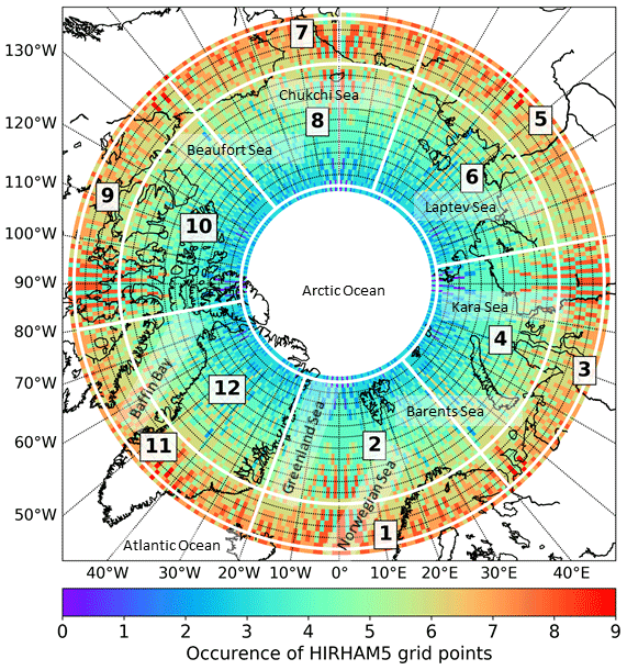
Figure 1The studied regions (described in Table 1) shown on the map with the occurrence of HIRHAM5 model grid points in the 1∘ × 1∘ sampling grid points.
Table 1The studied 12 regions divided equally in longitude with 60∘ to have the same sampling size between the different regions and in latitude divided into two latitude rings to examine the southern and northern parts of the Arctic separately. The last column shows statistically coinciding HIRHAM5 model run times with the CloudSat overpasses.
2.1 HIRHAM5
The HIRHAM RCM is based on the dynamics of the High Resolution Limited Area Model (HIRLAM; Undén et al., 2002) and the physical parameterizations of the atmospheric general circulation model ECHAM (Roeckner et al., 2003). We utilize here version 5, which combines HIRLAM model release 7.0 with ECHAM model release 5.2.02 (Christensen et al., 2007). HIRHAM5 has been applied to various Arctic studies (recently, e.g., Akperov et al., 2019; Sedlar et al., 2020; Inoue et al., 2021).
HIRHAM5 is run at a horizontal resolution of 0.25∘ (about 27 km) on a rotated latitude–longitude grid with the North Pole on the geographical Equator at 0∘ E and with 40 vertical levels. The altitude ranges from about 10 m above the surface up to 10 hPa, and the lowermost 1 km is represented by 10 levels. In this study, the daily snowfall rate constructed from the 3-hourly output is used for the observation-to-model approach. On the other hand, the 3-hourly output of the thermodynamic state and the mass mixing ratios of cloud ice, cloud liquid, snow, and rain are used to calculate synthetic reflectivities in the model-to-observation approach. While cloud ice and liquid mixing ratios are prognostic variables in the model, snow and rain are diagnostic variables.
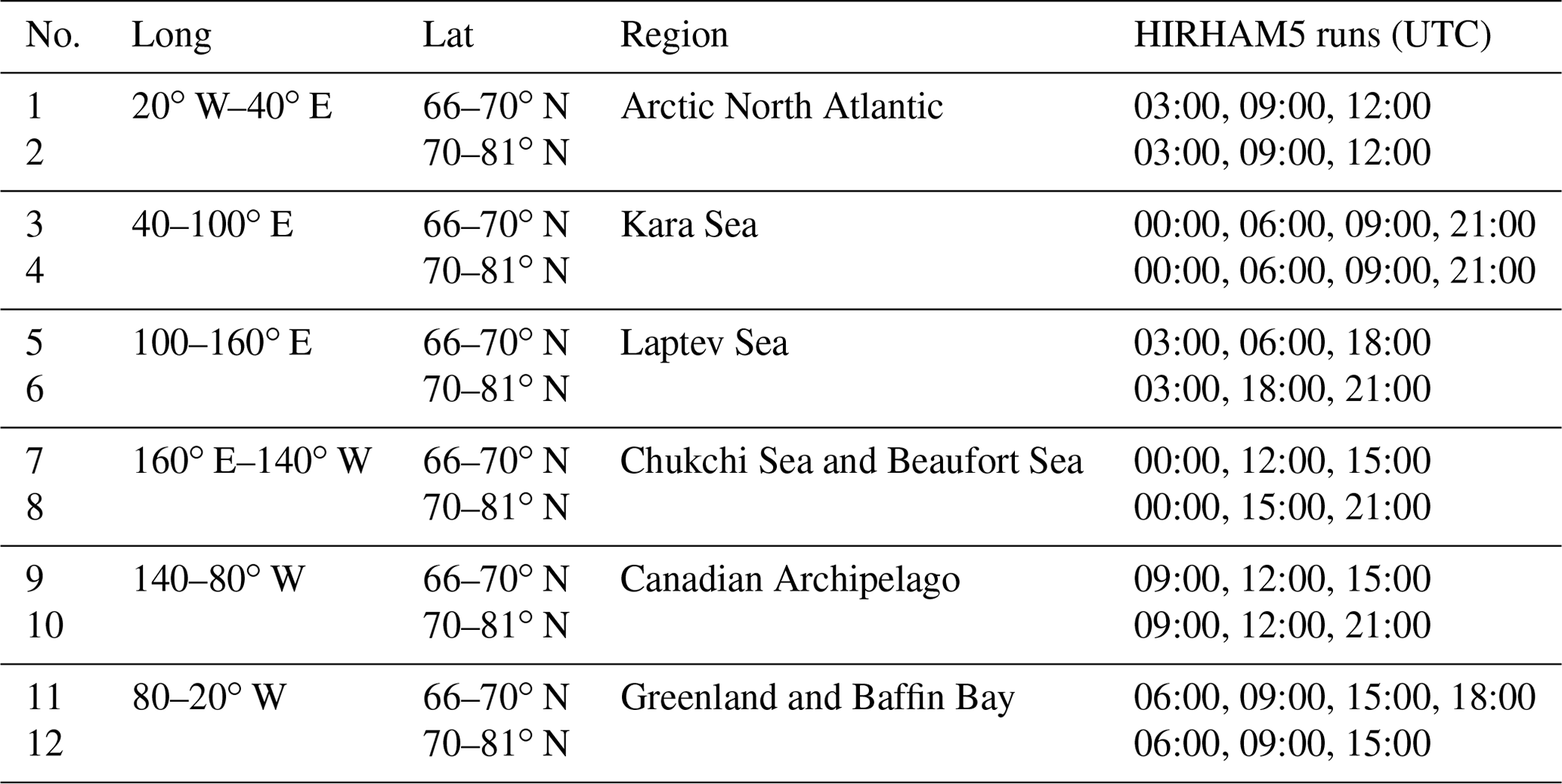
We apply at every time step a grid point nudging, i.e., dynamical relaxation (sometimes also called indiscriminate nudging or grid relaxation), which was originally developed for data assimilation (Omrani et al., 2012). We have chosen a parameter value corresponding to 1 % nudging. This ensures constrainment of the simulated large-scale flow to the driving ERA-Interim reanalysis. For an evaluation of HIRHAM5 snowfall using observations, the simulations must stay reasonably close to the real development of the synoptic weather situation, allowing us to separate dynamical from microphysical effects. Due to the nudging, the large-scale snowfall patterns are expected to correspond with reasonable accuracy to the observations, as is demonstrated in a snowfall case study for 7 March 2010 in Figs. 2 and A1. The location of the precipitation system and its vertical extent are rather similar in HIRHAM5 and CloudSat observations. Therefore, it is assumed that the differences between the modeled snowfall and observations are to a lesser degree related to the simulated large-scale flow but are mostly caused by the ECHAM5 boundary layer and microphysical parameterization employed in HIRHAM5 and observational uncertainties.
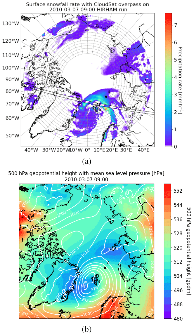
Figure 2Case study on 7 March 2010. (a) The overpass of CloudSat, where the surface snowfall rate (mm h−1) taken from the closest model run of HIRHAM5 is shown underneath and the overpass is colored with surface snowfall rate values of the 2C-SNOW-PROFILE product. Panel (b) shows HIRHAM5 500 hPa geopotential height with mean sea level pressure plotted with contour lines.

Figure 3Annual mean snowfall rates during 2007–2010, (a) modeled with HIRHAM5 when periods of CloudSat overpasses are considered and (b) observed with CloudSat and retrieved with the 2C-SNOW-PROFILE product, (c) the difference of snowfall rates between HIRHAM5 and CloudSat, and (d) the difference of the modeled snowfall rates with HIRHAM5, with and without considering the times of CloudSat overpasses. In panel (c) is the difference plot: the red colors show that HIRHAM5 has higher rates, whereas blue colors indicate that CloudSat provides higher rates. Percentages are calculated related to CloudSat observations. The thicker black line in (c) shows the latitude band of 72–73∘ N. In panel (d) is the difference plot: the red colors indicate that considering the times of CloudSat overpasses when calculating the mean shows higher rates and blue colors that, when using all daily modeled values, the mean is higher. Percentages are calculated related to model-only values. The sections marked in panel (d) show the two sub-regions in the northern North Atlantic for the CWT analysis (Sect. 4.2).
Unless specified, HIRHAM5 uses the modified Tompkins cloud scheme (Klaus et al., 2016) throughout the whole paper. However, to study the effect of different cloud cover schemes, we have also run the model for the studied period with two other schemes: the original Tompkins (Tompkins, 2002) and Sundqvist (Sundqvist et al., 1989) cloud schemes. The Sundqvist scheme is based on relative humidity; i.e., a critical threshold of relative humidity controls the cloud cover formation. The threshold decreases exponentially from 90 % near the surface to 70 % at higher altitudes. The Tompkins scheme is a prognostic statistical cloud scheme. The subgrid-scale variability of total atmospheric water content is specified by a probability density function in terms of the beta distribution. The higher-order moments of the beta distribution, namely, variance and skewness, are included and linked to subgrid-scale processes like turbulence, convection and microphysics. Fractional cloud cover is computed as an integral over the supersaturation part of the actual beta distribution. The Tompkins scheme includes adjustable parameters, which determine the shape of the beta distribution and microphysical processes (e.g., the aggregation rate – the efficiency of snow formation by aggregation of cloud ice particles). Klaus et al. (2016) found that a parameter tuning of the cloud ice threshold controlling the efficiency of the Bergeron–Findeisen process, combined with a scheme extension which allows negatively skewed beta distributions, is most suitable for Arctic cloud simulations. They showed that this modified Tompkins scheme significantly reduces Arctic cloud cover, in better agreement with CloudSat/CALIPSO observations. The more efficient Bergeron–Findeisen process decreases (increases) the cloud water (ice) content.
2.2 ERA-Interim
ERA-Interim is a global atmospheric reanalysis produced by the ECMWF (Dee et al., 2011). It was widely used as a reference, covering the period from 1 January 1979 onward until 31 August 2019, and was replaced by the ERA5 reanalysis, also available from 1 January 1979 onward. The system includes a four-dimensional variational analysis (4D-Var) with a 12 h analysis window. The spatial resolution of the data set is approximately 80 km (T255 spectral) on 60 levels in the vertical from the surface up to 0.1 hPa (Dee et al., 2011). To improve and constrain the forecast, surface, radio-sounding, and airborne observations as well as satellite measurements are assimilated into ERA-Interim (Dee et al., 2011). However, CloudSat observations are not applied, nor are the direct precipitation observations from any source. The cloud microphysics scheme utilized in ERA-Interim is based on Tiedtke (1993), representing clouds in terms of two prognostic variables. One variable is for cloud fraction and the other one for total cloud condensate, which in turn is divided into separate liquid and ice categories diagnostically according to temperature (Forbes et al., 2011). ERA-Interim is used here as lateral forcing as well as for the nudging for the HIRHAM5 simulations. Comparing both HIRHAM5 and ERA-Interim surface snowfall rates with CloudSat retrievals allows us to assess the influence of HIRHAM5 cloud and precipitation treatment. Mean snowfall rate for ERA-Interim is calculated from the monthly accumulation from the twice-daily values. Note that HIRHAM5 simulations were carried out before the release of ERA5.
2.3 CloudSat observations
CloudSat is part of the NASA A-Train (Stephens et al., 2002) constellation in a sun-synchronous orbit with an inclination of 98.2∘. Therefore, it provides nearly global coverage, reaching 82.5∘ from south to north (Tanelli et al., 2008) by a 16 d repeat cycle. The onboard Cloud Profiling Radar (CPR) operates at 94 GHz, providing observations of the vertical distribution of clouds and light precipitation with the vertical resolution (bin) of 240 m (Tanelli et al., 2008). Its footprint is 1.4 km across and 2.5 km along track. The minimum detectable reflectivity is dependent on, e.g., cloud cover, seasonal changes in temperature, surface type, and atmospheric attenuation, typically varying by ∼ 1 dB over the globe in the range from −30.9 to −29.9 dBZ (Tanelli et al., 2008), and the measurement uncertainties related to noise range from 3 dBZ for a reflectivity of −30 dBZ to about 0.1 dBZ for reflectivities above −10 dBZ (Wood and L'Ecuyer, 2018). Due to the relatively high frequency, the CPR signal can suffer from attenuation of atmospheric gases, e.g., of water vapor and oxygen. In addition, significant attenuation is also caused by the hydrometeors, and the measurements may be affected by the multiple scattering effects (Mace et al., 2007; Marchand et al., 2008; Battaglia et al., 2010).
Here, we use two CloudSat products, the measured radar reflectivity vertical profile 2B-GEOPROF (Marchand and Mace, 2018) and the snow profile product 2C-SNOW-PROFILE (Wood and L'Ecuyer, 2018). Version 5 (R05) is used for both products. 2B-GEOPROF includes the observed reflectivity corrected with the MODIS (Moderate-Resolution Imaging Spectroradiometer) cloud mask product (Ackerman et al., 1998). The measured reflectivity may be attenuated, which is not compensated in the product itself. Hence, in model-to-observation comparison, the attenuation due to atmospheric gases and hydrometeors is included in the reflectivity computations (Sect. 2.4). The 2C-SNOW-PROFILE product includes estimates of particle size distribution and snowfall rate retrieved from the observed radar reflectivity applying ancillary meteorological information of ECMWF-AUX (Stephens et al., 2008) and a priori information of snow microphysical and scattering properties (Wood and L'Ecuyer, 2018). In the 2C-SNOW-PROFILE product, the precipitation presence and phase at the surface are primarily examined from an additional 2C-PRECIP-COLUMN product (Haynes, 2018) and secondarily defined from the 2B-GEOPROF near-surface reflectivity values with the cloud mask correction and temperatures from ECMWF-AUX, for each radar profile within the retrieval algorithm. The snowfall is indicated, and a snowfall rate is retrieved if the assessed melted fraction of precipitation is lower than 10 %.
The retrieval of the snowfall rate (S) from the measured reflectivity (Z) is a significant source of uncertainty when applying radar measurements to estimate snowfall rates, e.g., Bennartz et al. (2019). Hence, in the 2C-SNOW-PROFILE product, the snow retrieval is not based on a single pair of parameter values of the Z–S relation but is optimized by minimizing a cost function which represents differences between simulated and observed reflectivities and also differences between estimated and a priori values of the snow microphysical properties (Rodgers, 2000; Wood and L'Ecuyer, 2018; Edel et al., 2020). Milani et al. (2018) found that adoptable Z–S parameterizations considering the local microphysical conditions provide better performance than a method with the static Z–S relationship. Thus, we are confident in using the output of the 2C-SNOW-PROFILE product as the ground truth while acknowledging the relevant unreliability stemming from the uncertainties in observed reflectivities, the used retrieval parameters and their a priori assumptions (Edel et al., 2020). The product has shown good detectability of light snow (snow water equivalent less than 1 mm h−1) but limited ability to retrieve at the higher end of snowfall intensity distribution (>1 mm h−1) when compared to the weather-radar-estimated surface snowfall rate (Cao et al., 2014; Norin et al., 2015). The relative uncertainty of the product increases with complex topography and higher frequency of mixed-phase precipitation (Edel et al., 2020).
As mentioned in Sect. 1, due to clutter contamination, the CPR cannot reliably measure reflectivity near the surface, resulting in the blind zone. The magnitude and vertical extent of the enhanced reflectivity values relating to back-scattered power from the surfaces vary depending on surface characteristics such as topography, roughness and material (Palerme et al., 2019). In the 2C-SNOW-PROFILE product, the blind zone is determined as the two (four) bins above the bin containing the surface over the ocean (land) and the next highest bin; i.e., an altitude of ∼ 750 m (1250 m) over the ocean (land) is considered for the snowfall retrieval (Wood and L'Ecuyer, 2018). Therefore, shallow precipitation or evaporation below this height might lead to a deviation from the true near-surface snowfall rate. The resulting underestimation (sometimes also overestimation) of snowfall rate due to a 1000 m blind zone has been found to be rather small for Svalbard but higher at the Belgian Princess Elisabeth station in East Antarctica (Maahn et al., 2014).
One of the important updates in the R05 product version is the use of an improved DEM (digital elevation model) for the estimation of the surface height, and this should affect especially Greenland, which has steeply varying terrain. With R05, the number of observations suspected of being contaminated by ground clutter should have decreased (Palerme et al., 2019). When applying the 2C-SNOW-PROFILE product, we have determined the surface snowfall rate from the snow profile data utilizing quality flagging of the snow retrieval status, following the example shown in Palerme et al. (2019) and Edel et al. (2020). The retrieval status is represented for each profile by an 8-bit array, and an activated bit provides information about the retrieval performance (Wood and L'Ecuyer, 2018). We have utilized only those profiles which have the zeroth and first bit field activated, indicating that a snow layer is detected in the profile and that snow is indicated at the surface. Additionally, if the third bit field is activated, meaning a large vertical gradient in snowfall rate between the near-surface bin and the bin immediately above is seen, the surface snowfall rate is determined from the second-lowest bin instead of the lowest near-surface bin. Such a strong gradient can be caused by surface clutter or by the presence of shallow precipitation. In the latter case, we underestimate the surface snowfall rate. However, the other two possible reasons, the mentioned ground clutter contamination or the partial melting, can produce a significant error into the estimated surface snowfall rate. Palerme et al. (2019) pointed out that the third bit field was mainly activated on the edges of the fjords over the eastern coast of Greenland and on the peaks of the Prince Charles Mountains expected to have clutter issues. Although orographic precipitation can also produce large snowfall gradients, in this case these flagged observations should cover larger areas along the ridges and coastline which were not observed by Palerme et al. (2019).
2.4 PAMTRA
PAMTRA (Mech et al., 2020) is a model framework to forward-simulate passive and active microwave radiation through the cloudy atmosphere for upward- and downward-looking geometries. It can calculate polarized brightness temperatures and the full radar Doppler spectrum and its moments. PAMTRA requires input that describes the atmospheric state, including hydrometeor contents and characteristics, instrument specifications, and the observation geometry.
In this study, the atmospheric state from HIRHAM5 was used to calculate the two-way gaseous attenuation of the radar beam using the gas absorption model by Rosenkranz (2015) including modifications of the water vapor continuum absorption (Turner et al., 2009) and the line width modification of the 22.235 GHz H2O line (Liljegren et al., 2005). To calculate the absorption/emission and scattering properties of hydrometeors, the hydrometeor mixing ratios have been converted to particle size distributions following the microphysical assumptions of HIRHAM5 (Appendix A). For each size, the back-scattering and extinction cross sections are calculated and used for simulation of the radar reflectivity. For cloud liquid and rain particles, which can be assumed to be spherical, the Lorentz–Mie method is used, and the refractive index of water is defined according to Turner et al. (2016). Cloud ice and snow particles have more complex structures than droplets or raindrops, and the spheroidal or spherical approximations do not provide realistic scattering characteristics at 94 GHz (Tyynelä et al., 2011). Hence, for these particles, the self-similar Rayleigh–Gans approximation (SSRGA; Hogan and Westbrook, 2014) is utilized, and the coefficients needed to describe the ice particle properties for the scattering computations are derived as in Hogan et al. (2017). The refractive index of ice is taken from Mätzler (2006). From extinction and backscatter cross sections, both the attenuated (by gases and hydrometeors) and unattenuated reflectivities have been calculated.
Multiple scattering may affect the observations (Battaglia et al., 2010) at 94 GHz and can be approximately 1 dB in snowfall with reflectivity values greater than 10–15 dBZ (Matrosov and Battaglia, 2009) but are not considered in these computations. PAMTRA includes a set of different options to describe particle size distributions from monodisperse, several functions and fully resolved distributions. To be consistent with the microphysical scheme of the atmospheric model or the in situ measurements that provide the input, PAMTRA implements the same assumptions for the particle size distributions and particle properties (Appendix A).
3.1 Sampling
HIRHAM5 model grid points and CloudSat CPR observations differ in space and time. These sampling differences need to be considered by spatial and temporal re-sampling in order to guarantee a fair comparison. The used sampling grid is an equal 1∘ × 1∘ grid. As stated in Souverijns et al. (2018), the CloudSat overpass occurring every couple of days is not representative for describing individual snowstorm variability in a certain specific location. However, with a large enough sampling grid, CloudSat can on average produce a reliable climatology.
Within the observation-to-model approach for each sampling grid point, one daily value is retained, taken as a mean of all the values of the CloudSat overpasses over the grid area and similarly for the HIRHAM5-modeled values. In case there are no CloudSat observations in the specific grid point, the daily value is excluded from the 4-year analysis, also from the model. Due to the CloudSat orbit, the grid points are observed at different preferable times of day, which is investigated in the model-to-observation approach (see below).
As the analysis is performed on the 1∘ × 1∘ grid, the number of model grid points per sampling grid cell decreases with latitude due to the meridian convergence (Fig. 1). Due to its orbit, the number of CloudSat measurements increases with latitude (Edel et al., 2020, therein Fig. 1). Therefore, for both data sets the frequency of occurrence per grid point is calculated and taken into account within statistical intercomparisons. When constructing joint histograms of temperature and reflectivity, so-called contoured frequency by temperature diagrams (CFTDs), the normalization is performed firstly by the number of samples in each grid point and secondly by the total sum of hits. In addition, the temporal sampling difference is considered by using the respective model output for each region closely coinciding with the times of the CloudSat overpasses. The stated model times for each region are shown in Table 1.
For the model-to-observation intercomparison, we also need to consider the different vertical sampling, i.e., equal spacing by CloudSat and a vertically stretched grid by HIRHAM5. Here, we defined the height bins as having a 250 m size below 1 km, a 500 m size between 1 and 4 km and a 750 m size between 4 and 10 km. The temperature bins are equally sized (2 K) between −70 and −10 ∘C. In our analysis, we have restricted the temperatures to below −10 ∘C to exclude any effect of melting and melting layer from the statistical analyses of modeled and observed reflectivities. The temperature values for the PAMTRA-modeled reflectivities are taken from HIRHAM5 itself, and for the CloudSat observations, temperatures are obtained from ECMWF-AUX (Miller and Stephens, 2001). The sensitivity of the CPR is approximately −28 dBZ, so the binning for reflectivities is carried out with 2 dBZ between −28.0 and 20 dBZ in the comparisons between modeled and measured reflectivity values. However, model-only analysis includes a wider range of values to demonstrate the small reflectivity values produced by cloud ice from the model, with more discussion in the results (Sect. 5.2).
3.2 CWT classification
To better identify reasons for potential deviations between observations and HIRHAM5, we also composite snowfall maps for different distinguishable weather regimes and evaluate the model output to observations in each regime separately as performed in Akkermans et al. (2012). Separating the daily modeled and observed snowfall rates according to an external parameter allows us to identify possible systematic model biases related to synoptic processes. In this study, we chose to investigate regimes of large-scale atmospheric circulation classified by strength, direction and vorticity of the geostrophic wind. We selected two sub-regions of the northern North Atlantic around Svalbard (Fig. 3d) covering the latitude band of 70–81∘ N. The eastern (40–10∘ E) and western (20∘ W–10∘ E) regions are considered such that the eastern region is directly north of Scandinavia and includes Svalbard, while the western region avoids land regions and is placed between Greenland and Svalbard. Both areas are characterized by high synoptic variability with frequent cyclone passages. The regime classification was performed with ERA-Interim 6-hourly 850 hPa geopotential height and shear vorticity for the studied period with the methodology of Jenkinson–Collison (Jenkinson and Collison, 1977; Philipp et al., 2016). The geopotential at 850 hPa is used to avoid topographic and boundary layer effects. The Jenkinson–Collision method is an automatic classification scheme (Philipp et al., 2016), where the geostrophic wind speed and vorticity at high/low central pressure are assessed in horizontally and isotropically arranged grid points and, based on threshold values, are set to eight exclusionary directional classes according to compass points (N, NE, E, SE, S, SW, W and NW) and two vorticity circulation regimes (cyclonic, C, and anticyclonic, AC) (Akkermans et al., 2012).
The daily regime classification of the two sub-regions (western/eastern) is specified with the cost733class software package of the COST Action framework (Philipp et al., 2016), and the occurrence of each regime for both sub-regions is determined. Clearly, the northerly, southerly and both vorticity classes are by far the most frequent, with occurrences of 16 % (25 %), 12 % (10 %), 31 % (38 %) and 34 % (32 %), respectively, for the eastern (western) sub-region. To simplify the analysis, the less frequent NE (6 % (7 %)) and NW (9 % (6 %)) were added to the northern regime, typically representing situations when cold Arctic air masses move southward. Similarly, SW (7 % (10 %)) and SE (8 % (3 %)) were added to the southern cluster, which is a typical situation for warm air intrusions into the Arctic. Finally, we divided the modeled and observed daily mean snowfall rates to these four regimes and calculated the contribution to the yearly mean snowfall rate to each regime separately.
4.1 Comparison of modeled and retrieved surface snowfall rates
Two distinct regions of high (>500 mm yr−1) average annual snowfall in the Arctic, namely, the southeastern coast of Greenland and the Atlantic storm track, are detected by both HIRHAM5 and CloudSat (Fig. 3). These are mostly related to cyclones which bring the heaviest snowfall during the snow accumulation season (September–May) in the regions of East Greenland, the Barents Sea, and the Kara Sea, which are the dominant regions of the extreme cyclone occurrence. Typically 20–40 events per one winter season take place (Rinke et al., 2017). The cyclone activity is much stronger in the Arctic Atlantic than in the Pacific; i.e., cyclone snowfall accounts for approximately 80 % of the total snowfall in these Atlantic regions, while cyclones account for only circa 50 % of total snowfall in the Pacific region (Webster et al., 2019). Additionally, lee cyclogenesis is important for precipitation production over southern and eastern Greenland (Rogers et al., 2004), whereas so-called Icelandic cyclones traveling further east are not favorable for precipitation over Greenland (Chen et al., 1997). This highlights the importance of the nudging in HIRHAM5 that leads to a good representation of cyclone-associated snowfall as depicted in Fig. 2. The lowest snowfall rates in both HIRHAM5 and CloudSat are located in the Beaufort Sea, the Canadian Archipelago, the central Greenland Ice Sheet, and eastern Siberia, with less than 100 mm yr−1.
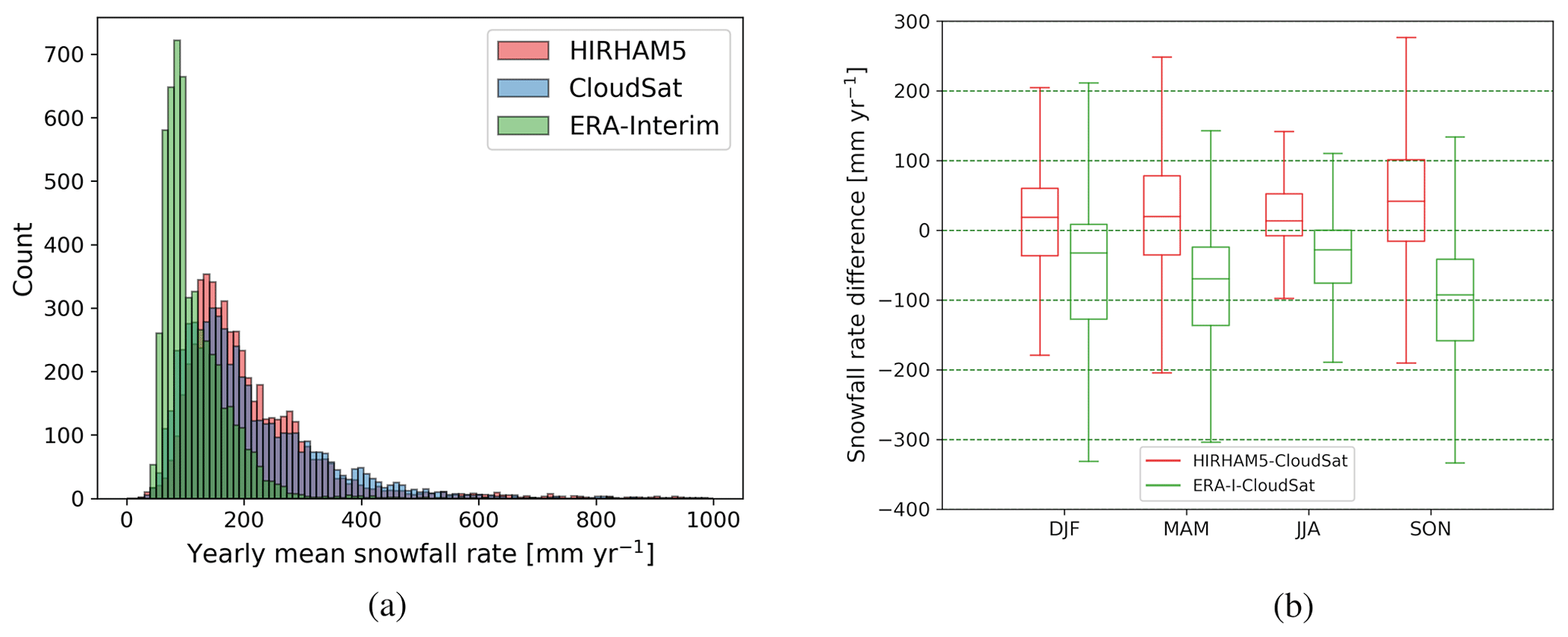
Figure 4(a) Histogram of yearly mean snowfall rates of HIRHAM5, CloudSat and ERA-Interim and (b) box plot of the difference in yearly snowfall rate between HIRHAM5 and CloudSat (red) and ERA-Interim and CloudSat (green) distributed seasonally. The box extends from the lower to upper quartile values, the line shows the median, and the whiskers show the range of the difference values as the first and third quartiles. The significance of the median difference for both HIRHAM5 and ERA-Interim compared to CloudSat observations is shown to be statistically robust for all seasons performing the Student's t test with random samples (10 % of the total amount) of the observed difference distributions.
Across the whole Arctic, the area-weighted domain average of the HIRHAM5 annual snowfall rate shows nearly perfect agreement with the CloudSat-based product, with 213 (214) mm yr−1 for HIRHAM5 (CloudSat). This value is also very similar to Edel et al. (2020), who derived 211 mm yr−1 as the CloudSat mean annual snowfall rate over the whole Arctic area when all profiles were included but a rate of 183 mm yr−1 when only profiles passing rigorous quality control were retained. Note that the studied area is different between these two studies. CloudSat and HIRHAM5 agree much better with each other than they do with ERA-Interim, which shows an annual area-weighted average Arctic snowfall rate of only 117 mm yr−1 in our study area (Fig. A2).
When looking at the frequency distribution of the annual mean snowfall rates over all grid points, a rather similar distribution with the highest occurrence of snowfall rates around 150 mm yr−1 is apparent for HIRHAM5 and CloudSat (Fig. 4a). As a minor difference, HIRHAM5 shows more often rates between 100 and 300 mm yr−1, whereas CloudSat has a tendency to higher extremes. The reasons for this could be the finer resolution of CloudSat-resolving local precipitation hotspots or clutter contamination. In contrast to HIRHAM5 and CloudSat, the coarser-scale ERA-Interim reanalysis has a much narrower frequency distribution, and its distribution has a maximum at only 100 mm yr−1. This demonstrates that, although HIRHAM5 is driven by ERA-Interim, snowfall is determined by its physical parameterizations, and these lead to an improved representation of snowfall.
We have proven that the chosen refined sampling has only minor effects on the results. That is, the difference in mean yearly snowfall rate between the model values coinciding with CloudSat observations and model-only values (Fig. 3d) is on average small over the whole Arctic region. For 92 % of grid points the difference is less than 20 %. When the coinciding sampling with CloudSat is applied, the modeled yearly snowfall rate is closer to CloudSat observations (the mean difference reduces from 2.2 to 0.7 mm yr−1).
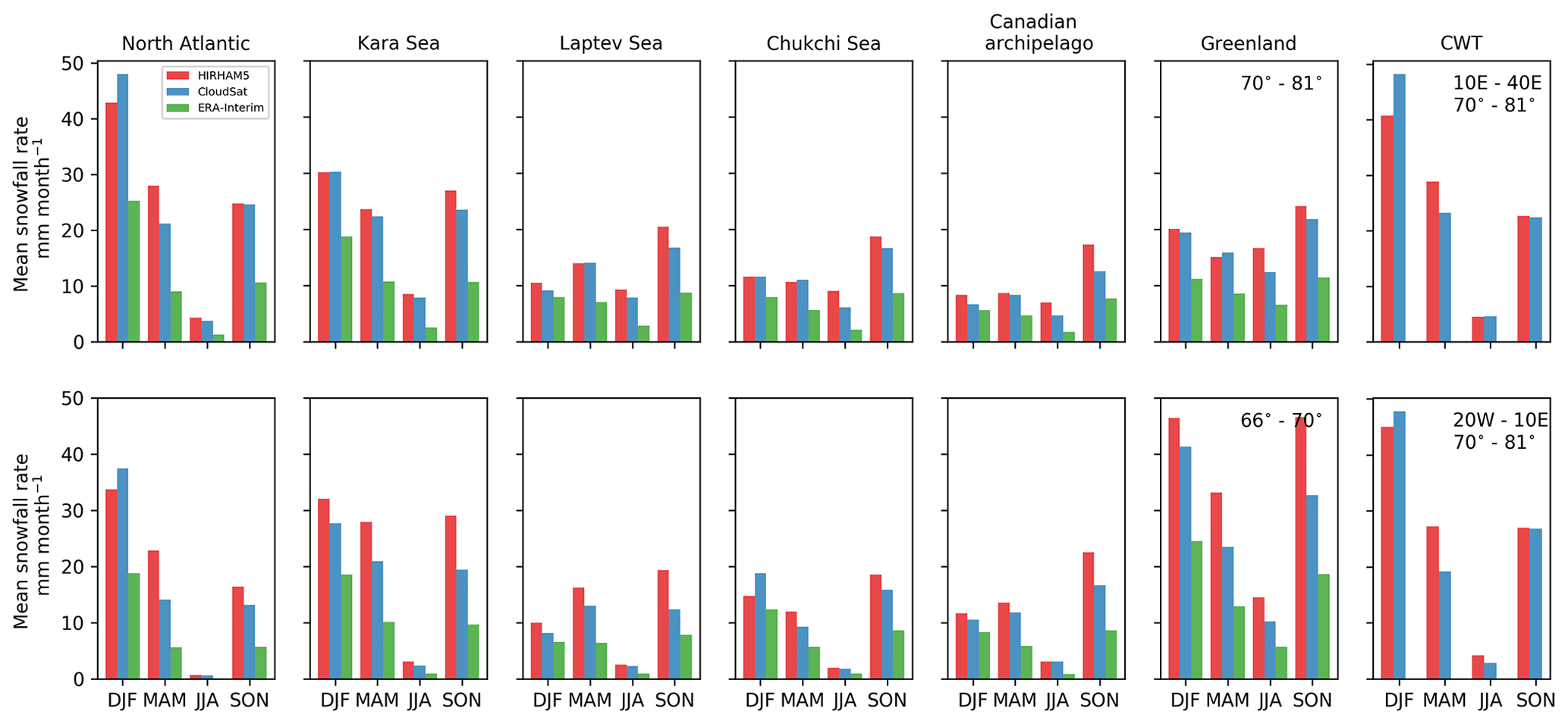
Figure 5Monthly area-weighted mean snowfall rates of HIRHAM5, CloudSat and ERA-Interim shown seasonally for each studied region. The latitude band 70–81∘ N is shown in the upper and the band 66–70∘ N in the lower panel. In the rightmost column, monthly area-weighted mean snowfall rates of HIRHAM5 and CloudSat are shown for both North Atlantic CWT regions.
Given the overall good agreement, we now look at spatial differences in the annual snowfall rate across the whole Arctic (Fig. 3c). Note that the observations by CloudSat are generally in line with the results of Palerme et al. (2019) and Edel et al. (2020). Though model and observations show similar spatial distributions, distinct spatial differences occur (Fig. 3c), and, e.g., root-mean square error in the yearly surface snowfall rates is high, at 148 mm yr−1 between HIRHAM5 and CloudSat and at 175 mm yr−1 between ERA-Interim and CloudSat. First, HIRHAM5 seems to consistently produce overly high orographic precipitation than is detected by CloudSat over the coastal mountains, e.g., in Greenland, Norway, Svalbard, Novaya Zemlya and the Putorana Plateau in Siberia. Therefore, this will also be investigated via the model-to-observation approach (Sect. 5), which allows a closer look at the vertical structure. Second, while in many areas differences seem to be of a random nature and can be attributed to the poor sampling by CloudSat, two larger areas with systematic differences also occur, namely, an underestimation of HIRHAM5 along the North Atlantic storm track, the Kara Sea, Baffin Bay and the Bering Strait and an overestimation of HIRHAM5 over Greenland.
The North Atlantic storm track region sticks out as the largest area of a systematic underestimation of HIRHAM5 (Fig. 3c). The underestimation is particularly strong southwest of Svalbard: the observed values are in between 500 and 1000 mm yr−1 here. In contrast, the model provides values of 400–700 mm yr−1 across this region. However, when studying the uncertainty in the CloudSat climatology in more detail, Edel et al. (2020) identified the Arctic North Atlantic region as having relatively large uncertainty, mainly due to a high frequency of possible mixed precipitation. In this respect it is important to look at the monthly resolved snowfall distribution (Appendix B, Fig. A3 for HIRHAM5, Fig. A4 for differences). From September on, the region of the highest snowfall in the North Atlantic moves more and more south with decreasing temperatures until its southern maximum extent in February/March. Interestingly, the highest model underestimation above 50 % (Fig. A4) over the Atlantic does not occur during the time of the strongest snowfall (January to March) but rather at the beginning of the snow season from September to November. This is reasonably in agreement with Akperov et al. (2018), who indicated an underestimated occurrence of deep cyclones in these months. Interestingly, this model underestimation seems to be coincident with the sea-ice-free areas of the North Atlantic and also Baffin Bay, as deduced from satellite data (Fig. A5) (Spreen et al., 2008). However, this is only a qualitative interpretation and requires more detailed examination in future studies. A clear statement whether and to what extent the HIRHAM5 underestimation in that region is related to model deficits or CloudSat uncertainty cannot be given yet.
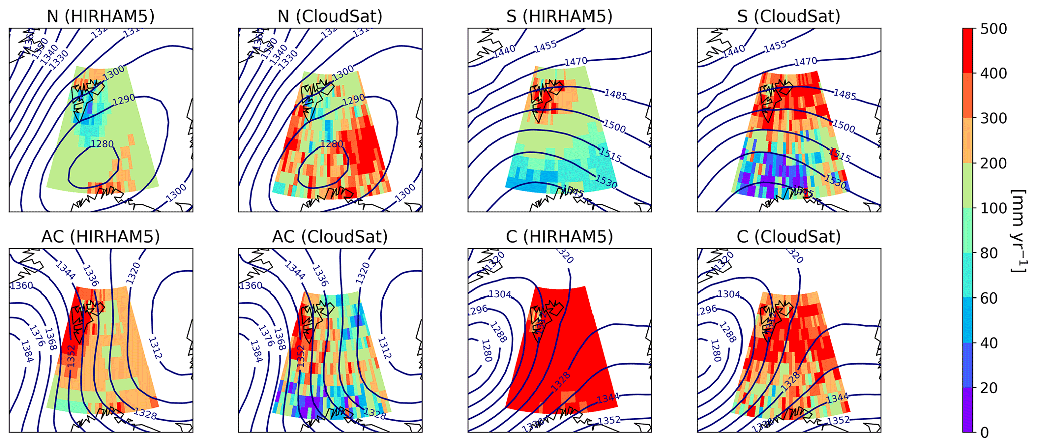
Figure 6Snowfall rate composited to different CWTs, N (including N, NE and NW), S (S, SE and SW), C and AC, for the area of 10–40∘ E (the colored sub-region is according to Fig. 3d) between latitude bands 70 and 81∘ N for both HIRHAM5 and CloudSat. The mean 850 hPa geopotential height (gpdm) associated with the CWTs is also shown as blue contour lines.
While for the region of southern Greenland a pronounced seasonal cycle in snowfall is evident, likely related to cyclone activity, this is not the case for the northern Greenland region (Fig. 5). A noticeable feature is the strong overestimation of the modeled snowfall rates over the Greenland Ice Sheet and the coastal mountainous regions in the southern part, as stated already in the yearly surface snowfall results (Fig. 3) (e.g., in the Greenland region with a median difference of 2.6 mm month−1 for the model to show higher values calculated over the whole year). However, it should be noted that total precipitation in North Greenland is rather low, and a high relative overestimation is not related to high snowfall rates. The annual distribution of the snowfall is similar to the detailed snowfall climatology from CloudSat over the Greenland Ice Sheet shown in Bennartz et al. (2019), even though the magnitude is overestimated by the HIRHAM5 model.
In general, the seasonal course of the snowfall rate for the different regions is well represented in HIRHAM5 as compared to CloudSat (Fig. 5). During the summer months, the model consistently overestimates the snowfall rates; however, the rates are also small in all regions, typically around 10 mm month−1 or less, except in Greenland, between 10 and 20 mm month−1. Again, the clear overestimation of the model is most visible during fall, especially in the lower-latitude band of the Kara Sea and Greenland regions. The North Atlantic (and the southern Chuckchi Sea) winter season sticks out as the only one where CloudSat shows higher snowfall rates than HIRHAM5. As discussed before, here too retrieval problems related to mixed-phase precipitation might occur, making it difficult to judge whether the model or the observations show deficits. The same also holds for effects of the blind zone, which therefore calls for an extended intercomparison in the observation space.

Figure 7The observed and modeled CFTDs for both latitude band regions in the winter season (DJF, 2007–2010). On the x axis is the reflectivity (dBZ), on the y axis is the temperature from −70 to −10 ∘C, and the normalization is done by the sum of total hits, which varies from region and season, but the total number of hits ranges between 86500 and 6.6×10⁶.
The model's underestimation of the annual snowfall rate distribution in the North Atlantic and the Kara Sea (Fig. 3c) is not visible in the region-wide averaged rates (Fig. 5), except in the winter season for the North Atlantic region. The reason lies in the averaging across the region. The model's overestimation over orographic and coastal areas (e.g., over the Scandinavian coast, Svalbard and Novaya Zemlya) masks the model's underestimation over the oceanic regions. To expand our study, we zoom into two distinct regions in the North Atlantic corridor for defining the CWT regimes introduced in Sect. 3.2.
4.2 CWTs
Because the strongest underestimation of HIRHAM5 surface snowfall rate is seen in the North Atlantic, we selected two smaller sub-regions (depicted in Fig. 3d) for the regime assessment with CWTs, namely, N, S, C and AC flow. The four different CWT regimes reveal consistently different snowfall distributions for both sub-regions (Fig. 6, Fig. A6). Both the HIRHAM5-modeled and CloudSat-observed surface snowfall patterns agree well, which can be explained by the nudging of HIRHAM5. Region-wide snowfall is brought in both sub-regions by cyclones which transport heat and moisture into the Arctic, and accordingly the C regime brings most of the snowfall for the region.
In the eastern sub-regions, during anticyclonic conditions (regime AC), a clear snowfall maximum northwest of Svalbard appears to decrease to the south and east in both HIRHAM5 and CloudSat. With the southerly flow the highest snowfall accumulation appears in the northern part of the region, generally above 76∘ N. During northerly flow, CloudSat shows that the majority of snow falls in the region southeast of Svalbard (Fig. 6), which is sensible, as this is a few hundred kilometers downwind of the ice edge, and convection needs time to fully develop when the cold air flows over the relatively warm ocean. For this CWT regime, HIRHAM5 shows nearly a factor of 2 underestimation in the maximum snowfall rates in the southeast of Svalbard, also seen in the mean snowfall rates in Fig. 5. Similar characteristics can be found for the western sub-region (Fig. A6). As both these sub-regions relate to the area of the largest underestimation southwest of Svalbard in the annual snowfall rate (Fig. 3), the poor representation of snowfall associated with northerly flow might be responsible for the overall HIRHAM5 underestimation. The northerly flow has a significant occurrence of 31 % 38 % for the eastern/western sub-region and is often associated with marine cold air outbreaks (MCAOs). MCAOs lead to organized convection when cold air flows over the relatively warm ocean, a phenomenon which many models struggle to represent (Geerts et al., 2022). The effect of underestimation during northerly flow might be partly compensated by cyclones which are associated with a higher snowfall rate in HIRHAM5 than in CloudSat.
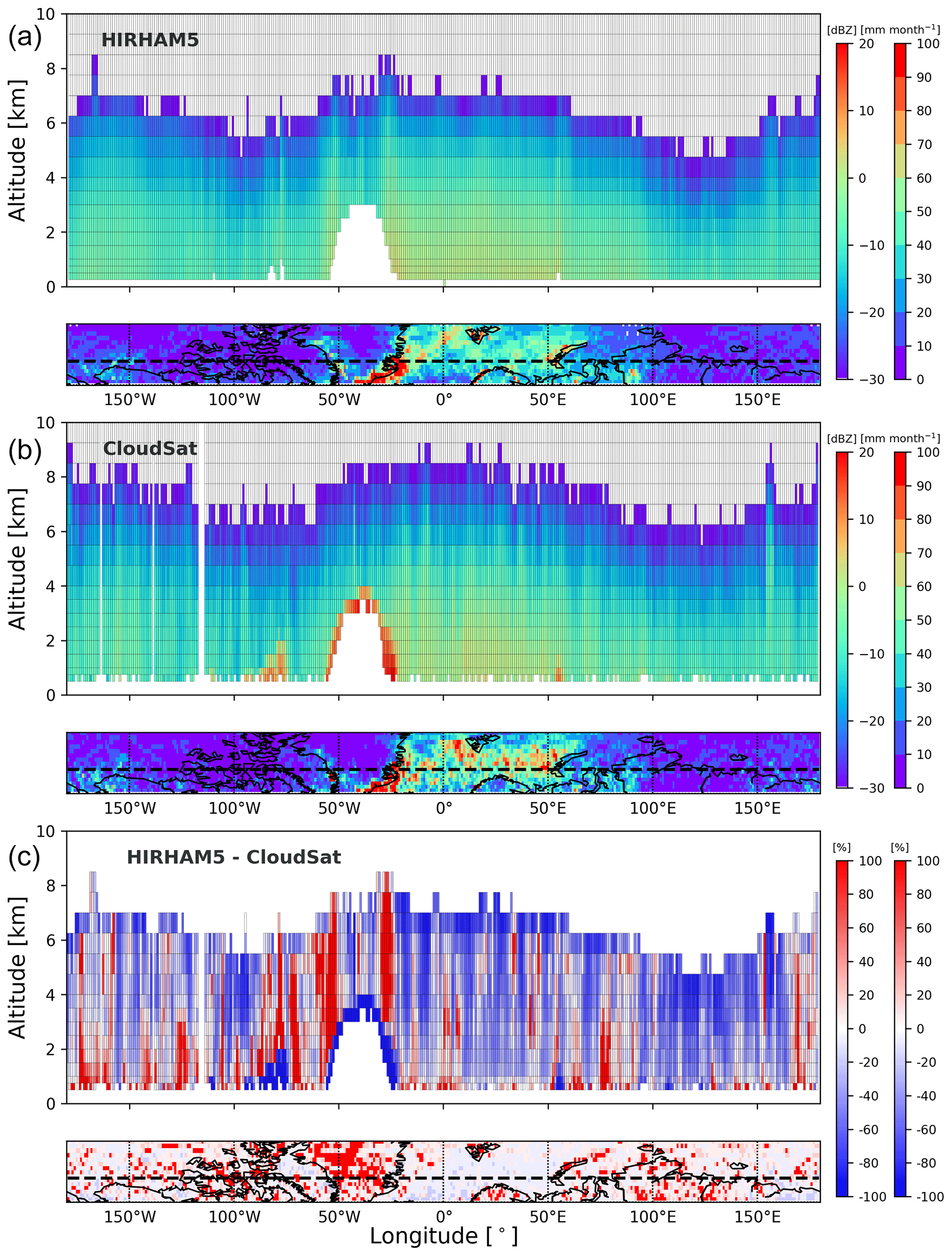
Figure 8Mean modeled reflectivity of all hydrometers of HIRHAM5 (a), observed by CloudSat, (b) and the difference of values (c) as a function of altitude for a latitude band of 72–73∘ N during winter (DJF). In the difference plot, the red color indicates that HIRHAM5 simulates a higher reflectivity than CloudSat observations, and blue colors vice versa. The small boxes below each of the reflectivity profiles show the monthly surface snowfall rates and the difference. The shown altitude is restricted to higher than 500 m, and the difference in percent is calculated by subtracting in linear scale the CPR-measured value from the modeled one, divided by the measured one, and multiplied by 100.
Utilizing the PAMTRA forward simulator, the HIRHAM5 model output of the mixing ratios of different hydrometeors can be converted to scattering properties, and the total simulated reflectivity can be compared to the one measured by CloudSat (2B-GEOPROF product; see Sect. 2.4) as described in Appendix A. This approach avoids assumptions in the snowfall rate retrieval from observations. Furthermore, it allows us to study the vertical structure of the hydrometeors, particularly with respect to orographic effects and the CloudSat blind zone. In this section, firstly we discuss the reflectivity distributions as a function of temperature for the different regions (Sect. 5.1) before we have a closer look at the factors which determine the vertical reflectivity profile (Sect. 5.2) and investigate the performance of employing different cloud schemes within HIRHAM5 (Sect. 5.3).
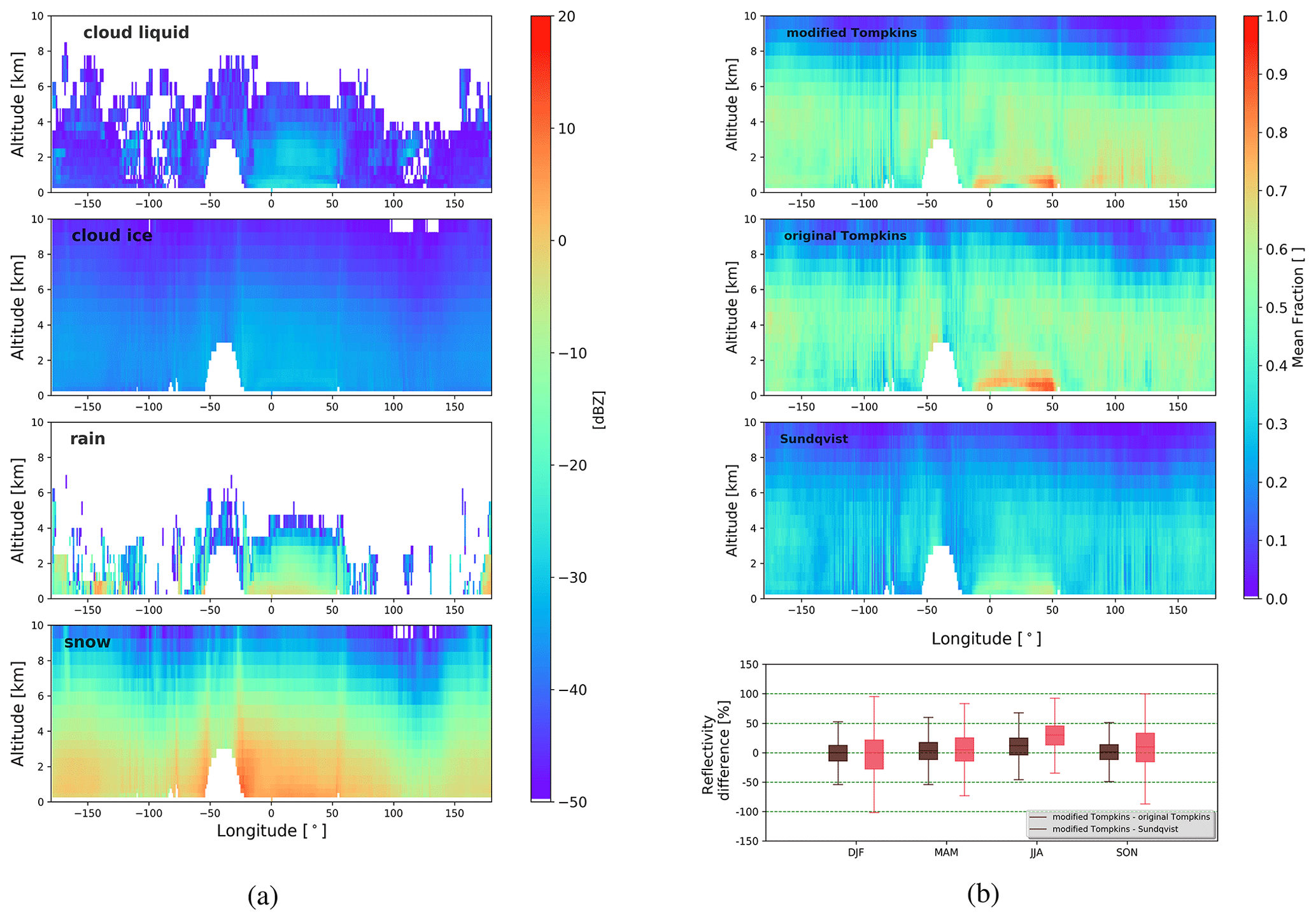
Figure 9(a) Mean modeled reflectivity with the modified Tompkins scheme separately for all hydrometers (cloud liquid and ice, snow and rain) as a function of altitude for a latitude band 72–73∘ N for the winter season (DJF). (b) The three upper panels show the mean fraction of reflectivity contributed by snow with the three different microphysical schemes in the winter season, and the lower panel shows a box plot of the reflectivity differences between the modified Tompkins scheme with respect to the two other schemes (difference from the original Tompkins scheme in brown and that from the Sundqvist scheme in rose) seasonally for snow. The significance of the median difference for both the original Tompkins and Sundqvist schemes from the modified Tompkins scheme is shown to be statistically robust for all seasons performing the Student's t test with random samples (10 % of the total amount) of the modeled difference distributions.
5.1 Regional differences in reflectivity profiles
To investigate the differences in the vertical reflectivity structure between the different regions, we focus on the winter season (DJF), which covers snowfall rates of approximately 30 % over all seasons. Furthermore, we reduce problems related to mixed-phase conditions as temperatures are generally low. The other seasons are shown in Appendix B. We follow Reitter et al. (2011), who build CFTDs instead of the often-used geometrical height, as this allows a better focus on the temperature-dependent cloud processes. CloudSat observations show the typical bi-modal structure in the CFTDs (Fig. 7) in nearly all regions with frequent occurrence of an ice cloud mode with low reflectivities around −20 dBZ at low temperatures of around −50 ∘C and a second mode associated with snow with reflectivities around 0 dBZ and temperatures warmer than −30 ∘C. Note that a minimum threshold of −15 dBZ is often utilized for identifying snowfall in the 2C-SNOW-PROFILE product (Wood and L'Ecuyer, 2018; Haynes et al., 2009).
As the transition from ice clouds to snow is seamless, a clear occurrence of a maximum following a linear slope from low reflectivities at cold temperatures to high reflectivities at warm temperatures is found in CloudSat observations (red line depicted in Fig. 7). This transition also reflects different snow growth processes, the depositional growth starting from around −50 ∘C and the dendritic growth zone at approximately −15 ∘C, leading typically through aggregation to enhanced snowfall rates. Also, different snowfall types such as shallow cumuliform and deeper nimbostratus snowfall events are associated with different CFTDs, as demonstrated by Kulie et al. (2016). Therefore, when averaging over larger regions and seasons, this linear pattern becomes dominant, as, for example, in the global CloudSat CFTD by Reitter et al. (2011). Clearly this behavior cannot be seen in the HIRHAM5 simulations. Hardly any reflectivities in regions colder than −35 ∘C are produced, indicating a problem with ice clouds which will be addressed in more detail in the next subsection.
Due to the lower occurrence (<0.1 %) of cold temperature reflectivities, reflectivities at warmer temperatures are relatively more frequent in HIRHAM5 than in CloudSat observations, with occurrences of >0.8 % for HIRHAM5 and with occurrences of between 0.6 % and 0.8 % for CloudSat. However, HIRHAM5 is able to reproduce regional differences seen by CloudSat correctly. Enhanced reflectivity related to the snow mode (−10 and 5 dBZ) occurs at the warmest temperature in the North Atlantic (around −10 ∘C) in both observations and model, similarly to slightly warmer temperatures in the Kara Sea region. In the Chukchi Sea, occurrences (0.4 %–0.8 %) are confined to a narrow temperature range between −20 and −35 ∘C, while in the Laptev Sea the distribution broadens to colder temperatures again in both observations and simulations. In the Chukchi Sea, HIRHAM5 can also reproduce the increased reflectivity occurrence (0.6 %) around −20 ∘C in the lower-latitude region compared to the higher-latitude region. The strongest difference between the observed and simulated CFTDs is visible for Greenland, where the simulations show reflectivities at much warmer temperatures (−20 to −10 ∘C) and higher reflectivities (0–10 dBZ), consistent with the overestimation in snowfall rate by HIRHAM5 discussed before.
We also checked the effect of attenuation in the simulations by comparing the attenuated reflectivity values to the non-attenuated values. The attenuated CFTDs are 5.1 % closer to the observed CFTDs and, generally, even with attenuation considered, the model sees higher reflectivities at warmer temperatures, except in the case of Greenland, where the observed occurrences of higher reflectivities are higher than the simulated ones. Additionally, the effect of using the modeled values concurrent with the expected CloudSat overpasses (Fig. 1 and Table 1) with respect to all modeled values is examined. Typically, differences show a random geographical distribution, in particular in regions where occurrences are low. The overall improvement in agreement is 0.8 % for the observed reflectivity values when only concurrent model values are used. Thus, the exact matching is considered insignificant except for times with little snow, such as in summer in some regions.
5.2 Vertical structure of hydrometeors
Because CFTDs average over different surfaces (ocean, sea ice, and land), we now investigate the vertical reflectivity structure for a latitude band of 72–73∘ N (circle indicated in Fig. 3c), again for the winter season. Figure 8 shows the seasonal mean reflectivity cross section along the latitude circle together with the mean surface snowfall rate to emphasize the reasons for strong snowfall in southeastern Greenland and across the North Atlantic Ocean. The importance of orography is clearly evident. HIRHAM5 shows orographic effects with reflectivity enhancement reaching mid-tropospheric levels at both coasts of Greenland and over the Baffin mountains and Novaya Zemlya. These structures are even more obvious in the differences from CloudSat, where HIRHAM5 shows strong overestimations (spikes) for nearly all grid points associated with strong orographic slopes. The strong vertical extent of these reflectivity signatures in HIRHAM5 is not visible in the observations and led us to conclude that this is a model deficit.
Looking at the CloudSat observations, the effect of ground clutter which causes a deeper blind zone over land (up to 1200 m) is most visible for Greenland and Baffin Island (with elevations up to 2000 m). Clutter filtering might cause the possible model overestimation over Greenland in winter (Fig. 5), which has also been found by (Edel et al., 2020) for the Arctic-wide average. Consistent with the CFTDs, reflectivities of more than −20 dBZ can be found in much higher (colder) parts of the atmosphere by CloudSat than in HIRHAM5, which will be investigated next.
5.3 Differences between the different cloud microphysical schemes
The simulated reflectivities can provide additional insight into the contributing portions of different hydrometeors to the total reflectivity. At first, we look at the HIRHAM5 control run employing the modified Tompkins scheme. Again for winter, we show the reflectivity by different hydrometeor types along the latitude belt in Fig. 9a. Snow particles clearly contribute the most to the simulated reflectivity for all heights and also throughout all the seasons. Even in summer (not shown), when the snow particles manifest higher in altitude to the reflectivity, their contribution to reflectivity dominates over that of rain particles. The highest reflectivity values due to rain particles are concentrated in the North Atlantic region (20∘ W–10∘ E), and some higher values are also modeled in the East Siberian Sea (150–180∘ E) and the Beaufort Sea (150–130∘ W). Cloud ice produces reflectivities over the full troposphere; however, these are rather low, in particular in the higher troposphere. This likely originates from the threshold of ice particle radius to be monodisperse of 40 µm (see Appendix A), which results in very low reflectivity values. In contrast, the smallest radius of a particle in the snow class is 0.1 mm, and, thus, snow always produces significant snow reflectivity.
Even in winter, cloud liquid water is present within the lowest 4 km and produces significant reflectivities close to the surface over the North Atlantic. During the summer months, their contribution is more widely distributed to the studied latitude ring and is higher in altitude (not shown), as is to be expected. The presence of low-level clouds and rain over the North Atlantic points to the difficulties in both (i) retrieving snowfall in mixed-phase conditions and (ii) simulating reflectivity, as melting might produce complex particles which are not taken into account in the forward simulation.
In addition to the control run with the modified Tompkins scheme, two more runs with different cloud microphysical schemes, i.e., the original Tompkins and Sundqvist schemes, are performed, and their results are compared (Fig. 9b). For all the schemes, the overall total mean reflectivity profile compared to the CloudSat-observed reflectivity profile is close to similar. The mean reflectivity difference from CloudSat varies between seasons and schemes, but generally the mean difference ranges between 0.3 % and 2.3 %, and no clear statement can be made as to which of the schemes in general would be closest to reproducing the total reflectivity values compared to observations.
However, there are distinct dissimilarities between the schemes when the contributions to reflectivity by different hydrometeors are examined (Fig. A10). The original Tompkins scheme seems to produce more cloud liquid particles than the modified Tompkins or Sundqvist scheme, similarly to stated in Klaus et al. (2016), connected to the enabled more enhanced Bergeron–Findeisen process and thus associated with an increase in cloud ice particles. The finding of Klaus et al. (2016) is limited over sea ice areas only, and this is not obvious from our analysis here over a lower-latitude band (72–73∘ N) from these model runs. Another difference is that the Sundqvist scheme produces rain particles, though small amounts, reaching high levels of the atmosphere, which is not the case with either of the Tompkins schemes. The notable dissimilarity between the schemes is the contribution of cloud ice and snow particles to reflectivity. As both Tompkins schemes seem to have a high fraction of snow particles, especially at the lower altitudes, the Sundqvist scheme tends to have higher fractions of cloud ice particles contributing even at the lower altitudes. The abovementioned scheme differences seem to be seasonally independent; i.e., similar features can be seen not only during winter, as shown in Fig. A10. While we do not go into more detail here, it is clear that the model-to-observation approach allows us to investigate the relative performance of different schemes. The next step would be to identify regimes, such as those based on temperature that show especially high differences between the cloud schemes, and subsequently compare observations and different model simulations for these regimes.
This study investigates how well a regional climate model, in this case HIRHAM5, can represent the Arctic snowfall both regionally and seasonally compared to the CloudSat-retrieved surface snowfall rates and observed reflectivity profiles. We identified the specific weather types related to surface snowfall rates and their patterns over the northern North Atlantic.
Firstly, in the observation-to-model approach, the modeled surface snowfall rate is compared to the 2C-SNOW-PROFILE product at yearly and monthly scales. The average yearly modeled snowfall rate (213 mm yr−1) agrees with the retrieved values (214 mm yr−1), and the spatial distributions are similar. This includes the patterns of the storm-track-related snowfall over the northern North Atlantic in winter and over Baffin Bay being seen in increased snowfall rates on the western coast of Greenland during fall. The seasonality of snowfall rates over the Siberian seas (lower in winter, higher in summer) is also represented well. One of the clear differences is found for the magnitude of the orographic snowfall over the (coastal) mountains, e.g., in Greenland, Norway, Svalbard, Novaya Zemlya and the Putorana Plateau in Siberia, where the model significantly overestimates the snowfall rates compared to CloudSat. Another difference is the underestimation of the magnitude of the snowfall rate over the northern North Atlantic in the model compared to CloudSat. This seems partly to be caused by the poor representation of MCAOs in the simulations and by CloudSat uncertainty related to mixed-phase precipitation over the open sea. Follow-up in-depth studies on this are required.
Secondly, in the model-to-observation approach, the model output is applied to the PAMTRA forward simulator to compute the reflectivity; i.e., the simulated reflectivity is compared to the CloudSat CPR-measured reflectivity (2B-GEOPROF product). The results support the surface snowfall rate findings. The model and observations show enhanced reflectivity over the storm track regions, especially over the northern North Atlantic during fall and winter. The observations of the Greenland surface layer and, e.g., the Baffin mountain range are clearly contaminated by the clutter. However, the modeled overestimation of orographic precipitation is also pronounced on the coasts. Generally, it seems that the modeled attenuation is higher than actually seen in the observations, especially during the summer months. This difference could also (at least partly) be explained by multiple scattering effects which would counteract attenuation (Matrosov and Battaglia, 2009). However, without considering attenuation in the simulations, the model overestimation increased by more than 10 %–20 %.
Based on the CFTD analysis, the CPR-observed reflectivity shows higher occurrences in the colder regime (i.e., at generally higher altitudes), while the modeled occurrences dominate at the lower altitudes (warmer temperatures). In the model, the threshold of the ice particle radius is 40 µm and, thus, the simulated reflectivity occurrences are often for the ice particles below the −30 dBZ threshold regime, and the snow growth process is inadequately depicted in the profile. The enhanced reflectivity during fall and winter at temperatures close to −10 ∘C (interpreted as close to the surface level) is seen in both the model and observations and indicates the frequent snowfall due to cyclone activity. Especially during fall, but also seen in the winter months, the observations show a pronounced bi-modal feature, possibly indicating different snow growth processes, the depositional and dendritic growths, and/or the presence of two different snowfall categories, the shallow cumuliform and thicker nimbostratus snowfall, studied in Kulie et al. (2016). Further analysis is needed to interpret the ice growth processes and related simulated reflectivities, as these were clearly one of the significant differences between the model and observed values. Additionally, the other CloudSat-retrieved products such as the classification of the 2B-CLDCLASS product could be used to investigate more detailed representation of the microphysical processes in the model.
For each grid point and model level, HIRHAM5 provides the mass mixing ratios of all hydrometeor classes: cloud ice and droplets and snow and rain particles. From the ratios, the particle size distributions (PSDs) are calculated as well as particle properties such as size, shape, and density, following the ECHAM5 microphysical assumptions, and are used as input into PAMTRA.
In HIRHAM5, all particles are basically assumed to be spherical and described with constant densities: for cloud droplets and rain particles ρw=1000 kg m−3, for ice particle ρi=500 kg m−3, and for snow particles ρs=100 kg m−3. The reference density of air is ρ0=1.29 kg m−3, and the density of dry air ρa is calculated at the corresponding height.
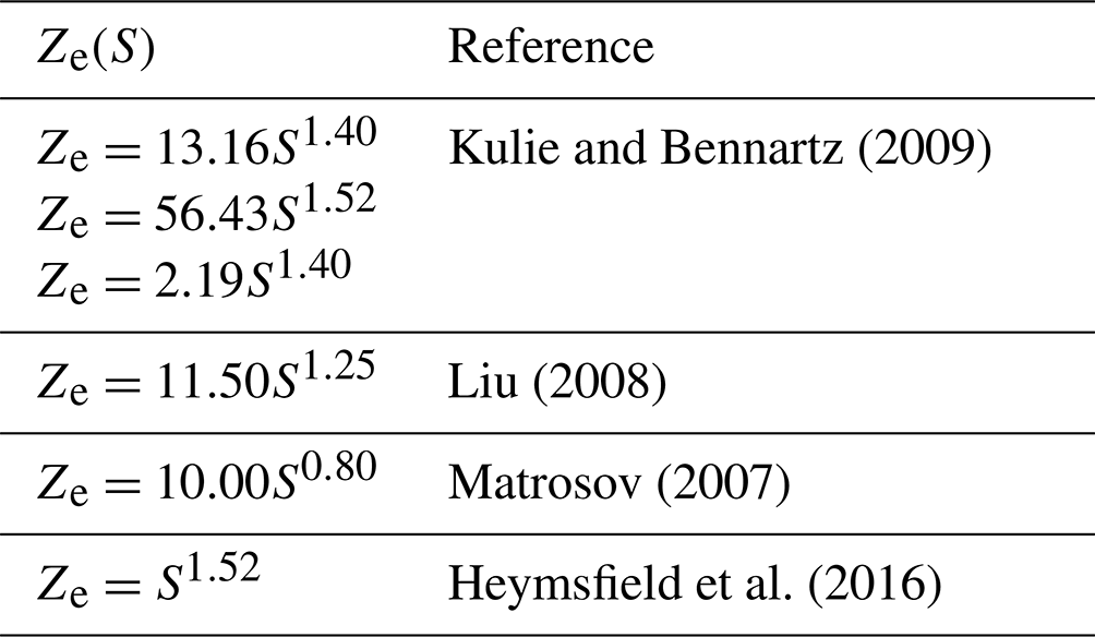
Kulie and Bennartz (2009)Liu (2008)Matrosov (2007)Heymsfield et al. (2016)Table A1The snowfall retrieval relations used in calculating the example profile in Fig. A1.
HIRHAM5 provides the mass mixing ratios ql and qi as prognostic variables for the cloud liquid and ice, respectively. The mean volume radius of cloud droplets can be obtained as in Roeckner et al. (2003) by
where the cloud droplet distribution Nl is assumed to have a monodisperse distribution declining exponentially between fixed values of the lower troposphere Nllt and the upper troposphere Nlut (Roeckner et al., 2003). Nl can be described as a function of pressure p (Pa) (Stevens et al., 2013):
where the pressure top value of plt=80 000 Pa for the lower troposphere is assumed. The fixed values for number concentrations depend on whether the air mass column is over land Nllt=220 cm−3 and over ocean ice Nllt=80 cm−3, and in the upper troposphere the value decreases to Nlut=50 cm−3, irrespective of surface type.
For cloud ice, the effective radius rei is determined with the mean volume radius rvi in meters (Levkov et al., 1992; Roeckner et al., 2003) defined as
and ice particle distribution Ni is also assumed to be monodisperse (Potter, 1991):
where Dvi is the mean volume diameter of ice particles.
For the precipitation, both snowfall and rain, HIRHAM5 output provides the fluxes divided into two components, large-scale and convective . The convective component was assumed to be small (constituting approximately less than 1 % in precipitation rate and the occurrence frequency an order of magnitude smaller) compared to the large scale, and therefore it is not considered in the forward simulations. The large-scale fluxes are converted to mass mixing ratios. For the snow mixing ratio,
where fractional cloud cover Cpr=1 is assumed and the velocity-dimensional parametrization of Heymsfield and Donner (1990), with a11=3.29 and b10=0.16, is employed. Hence, the slope of snow particle size distribution can be determined as in Potter (1991):
where the exponential snow particle distribution of Gunn and Marshall (1958) is followed by a constant intercept parameter m−4. For the snow class, a minimum ice crystal size is set to m.
The raindrop size distribution follows the Marshall–Palmer distribution with a value of m−4 (Marshall and Palmer, 1948), and the mass mixing ratio qr and slope parameter λr can be defined as follows:
and
where fall velocity of raindrops is parameterized according to Kessler (1969):
with Cpr=1 and a10=90.8.

Figure A1Case study on 7 March 2010. In panel (a), above is a reflectivity simulated by PAMTRA with the mixing ratios produced by HIRHAM5 and below is the observed reflectivity of CloudSat. In panel (b), it is shown for the profile location marked as a black solid line in panel (a); on the left are the profiles of reflectivity with CloudSat (red line), modeled (blue line), and example values from the literature (stated in Table A1) with the corresponding snow mixing ratio (gray dashed lines), in the middle are cloud liquid (light green), ice (light blue), rainwater (green) and snow equivalent liquid (blue) contents, and on the right are the different mean diameter profiles for the hydrometeors, i.e., mean volume diameter of cloud liquid (light green) and ice (light blue), median volume diameter of rain (green) and snow particles (blue).
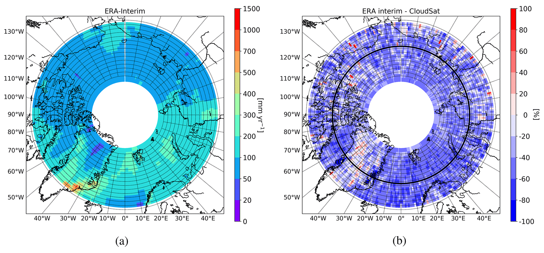
Figure A2(a) Yearly mean snowfall rate of ERA-Interim. (b) Difference of snowfall rates between ERA-Interim and CloudSat. In (b) the difference plot, the red colors show that ERA-Interim has higher rates, whereas blue colors indicate that CloudSat provides higher rates. Percentages are calculated related to CloudSat observations.
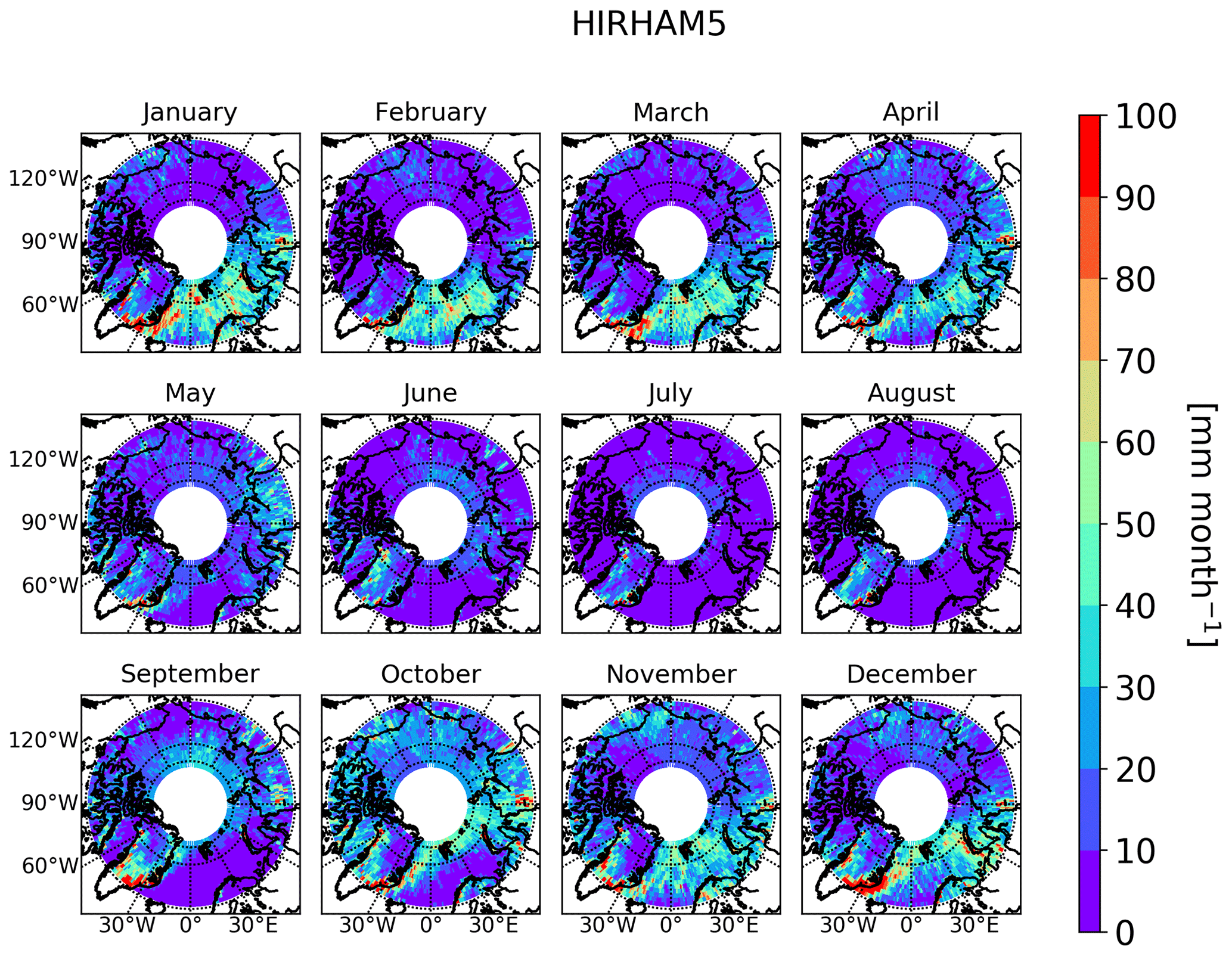
Figure A3Monthly mean snowfall rate of HIRHAM5 when using the values coinciding with CloudSat observations.
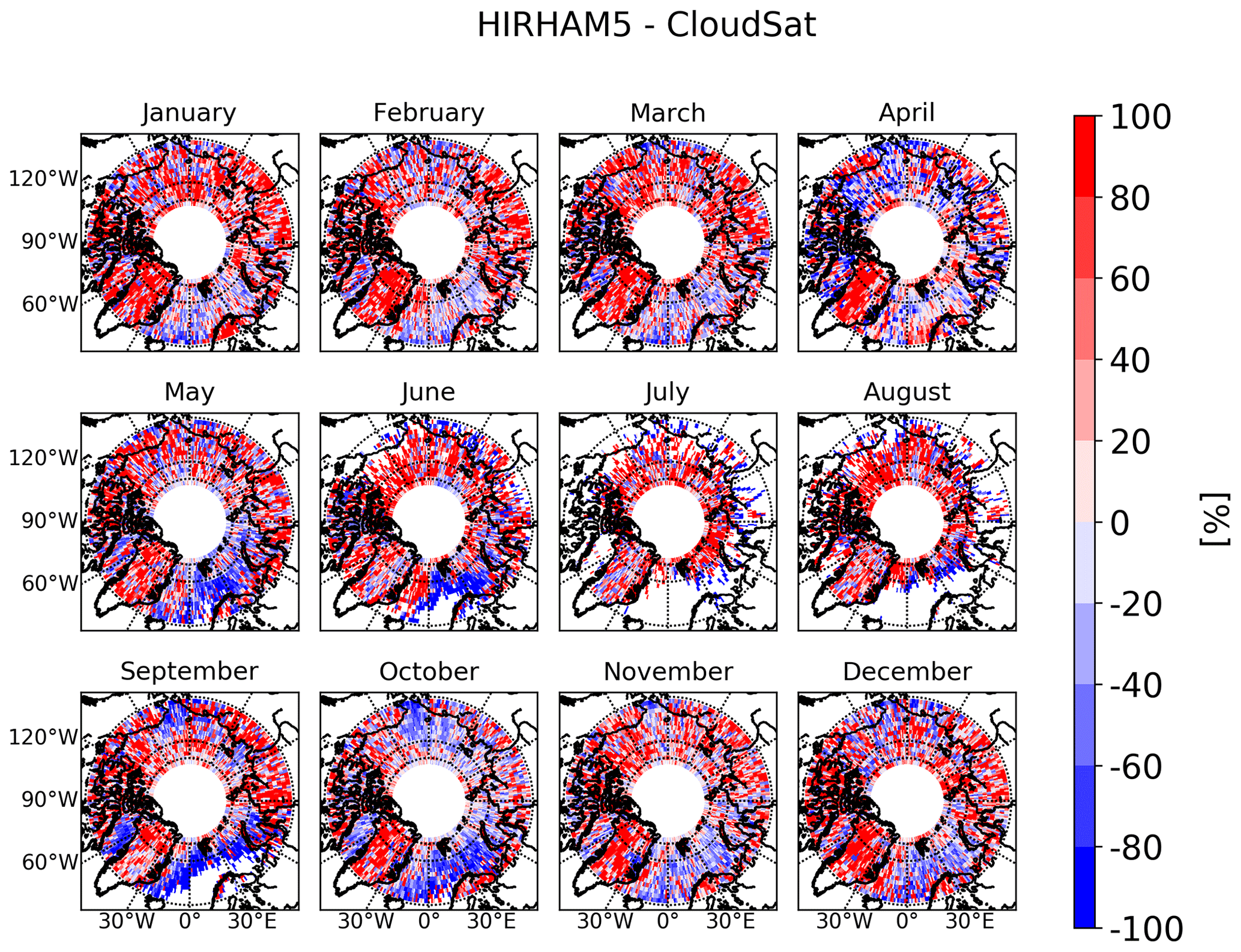
Figure A4Difference of the monthly mean snowfall rates (%) of HIRHAM5 and CloudSat. Here with red colors HIRHAM5 shows higher rates, whereas with blue colors CloudSat observes higher rates. Percentages are calculated related to CloudSat observations.

Figure A5The monthly sea ice extent is defined from space-borne observations of AMSR-E/AMSR2 on a 6.25 km grid (Spreen et al., 2008) for the studied period.
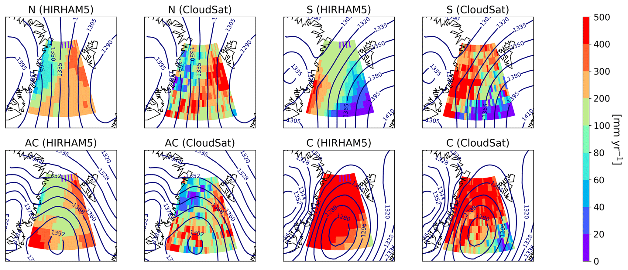
Figure A6Snowfall rate composited to different CWTs, N (including N, NE, and NW), S (S, SE, and SW), C and AC, for the area of 20–10∘ E between latitude bands of 70–81∘ N for both HIRHAM5 and CloudSat (the colored sub-region is according to Fig. 3d). The mean 850 hPa geopotential height (gpdm) associated with the CWTs is also shown as blue contour lines.
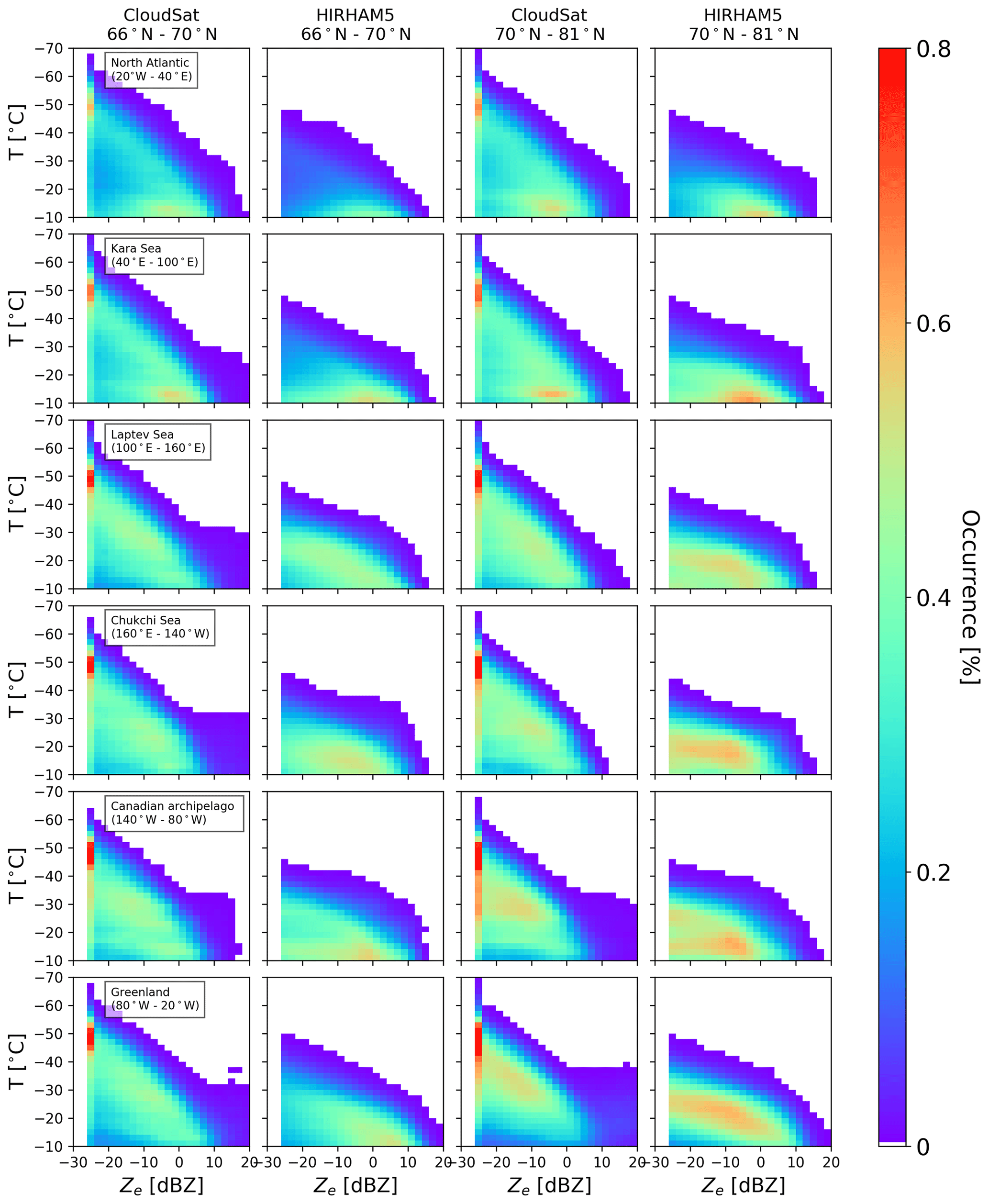
Figure A7The observed and modeled CFTDs for both latitude band regions in the spring season (MAM, 2007–2010). On the x axis is the reflectivity in dBZ, and on the y axis is the temperature from −70 to −10 ∘C. The normalization is done by the sum of total hits.

Figure A8The observed and modeled CFTDs for both latitude band regions in the summer season (JJA, 2007–2010). On the x axis is the reflectivity in dBZ, and on the y axis is the temperature from −70 to −10 ∘C. The normalization is done by the sum of total hits.
Figure A9The observed and modeled CFTDs for both latitude band regions in the autumn season (SON, 2007–2010). On the x axis is the reflectivity in dBZ, and on the y axis is the temperature from −70 to −10 ∘C. The normalization is done by the sum of total hits.
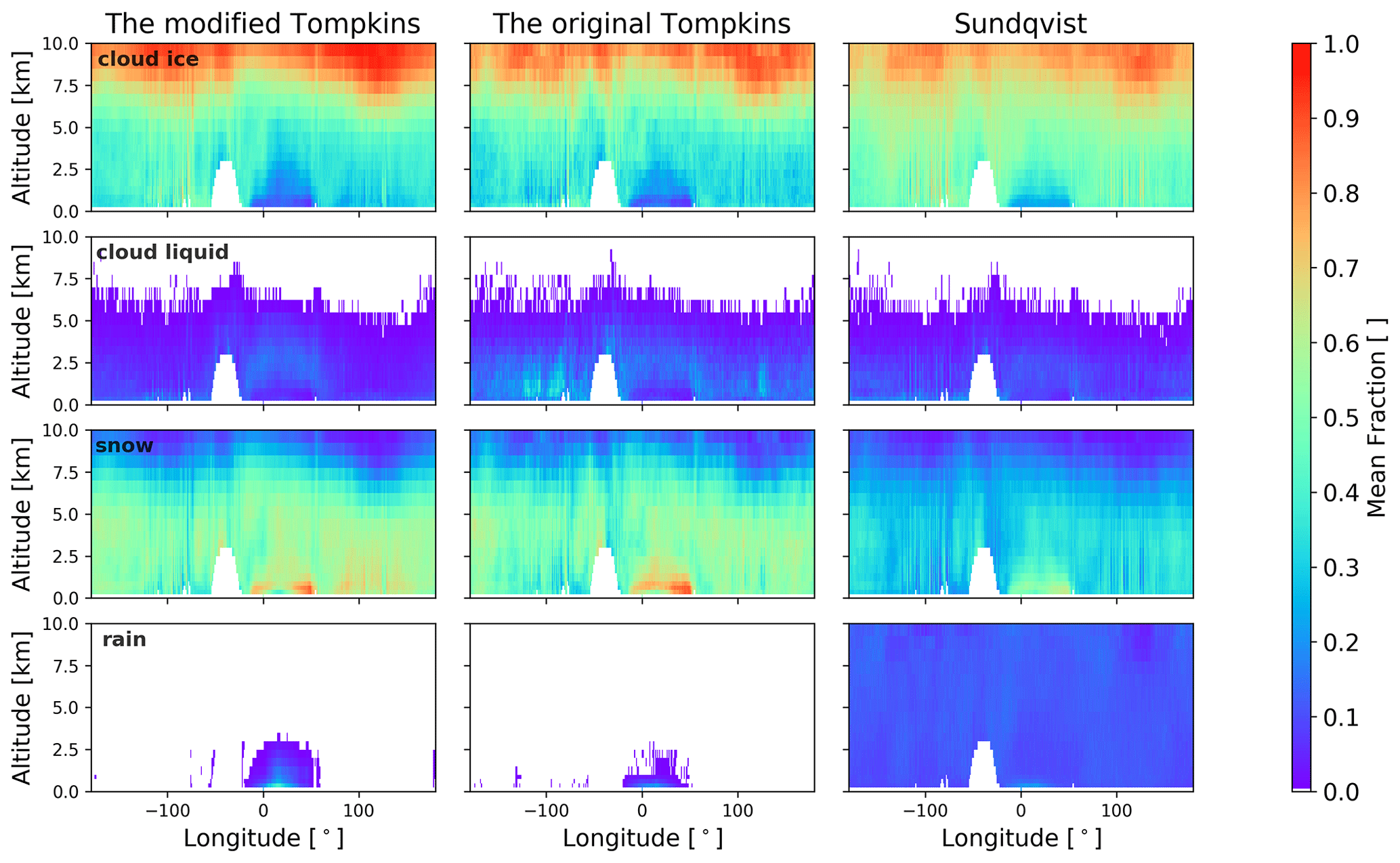
Figure A10A mean fraction of reflectivity contributed by the different hydrometeors as a function of altitude for a latitude band of 72–73∘ N in winter (DJF) for the different microphysical schemes, the modified Tompkins (left panel), original Tompkins (middle panel), and Sundqvist (right panel) schemes, respectively.
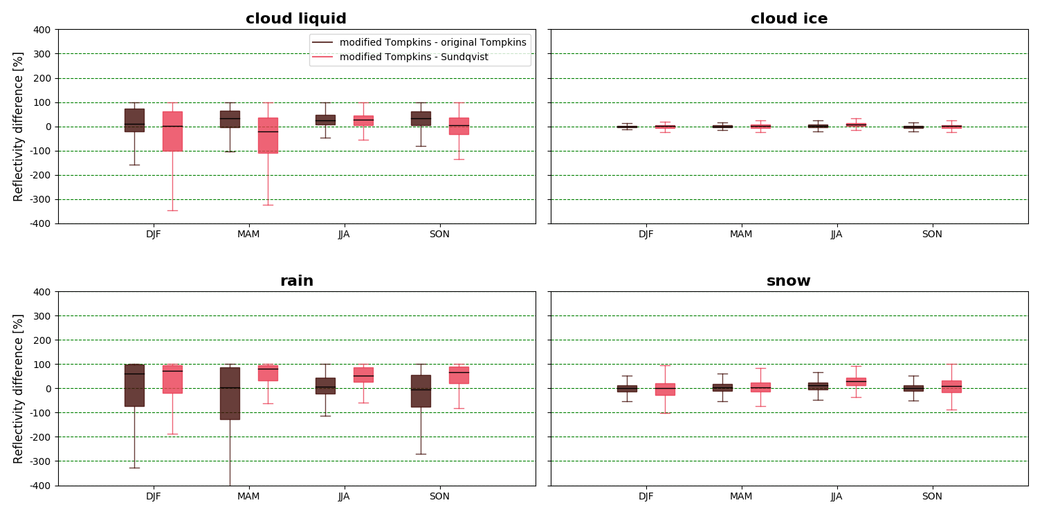
Figure A11The box plot shows the differences in percent between the modified Tompkins scheme with respect to the two other schemes for different hydrometeors distributed seasonally.
This section includes the additional figures to demonstrate the wider picture of the analysis in comparing the HIRHAM5 outputs to the CloudSat snowfall retrieval results and reflectivity observations. Figures are mainly referred to in the main text.
As an example, a simulated radar reflectivity cross section is shown in Fig. A1a together with its observational counterpart for a satellite overpass on 7 March 2010. The surface clutter is well distinguished in the CloudSat observations, especially over Greenland. The cut-off threshold of −28 dBZ following the sensitivity of CPR is applied for both simulations and observations. Generally, the agreement in the vertical structure of precipitation is good. Due to the lower spatial resolution of the model, the simulated clouds are more widespread than those observed. However, differences in the magnitude and cloud top height are evident.
In Fig. A1b, the snowfall retrieval results calculated with the PAMTRA simulator are compared to the known retrieval values from the literature for one representative profile during a precipitating event. This is performed more or less as a sanity check for the scattering assumptions in PAMTRA and how close the scattering computations are to the values reported in the literature (Table A1). Though the simulated reflectivity is slightly underestimated over the full profile, the large differences occur in the upper troposphere, which is likely due to cloud ice. There is hardly any cloud ice above 6000 m in HIRHAM5, and thus cloud height seems to be lower for the simulated reflectivity than for the observed reflectivity. Actually, the HIRHAM5 model has an intrinsic upper threshold for the size of cloud ice particles with a diameter of 40 µm. With this size, the calculated back-scattering cross sections for ice particles result in reflectivity values below the cut-off threshold defined by CPR.
In HIRHAM5, the ERA-Interim reanalysis is used with the grid point nudging to control the simulated large-scale flow; however, as the modeled snowfall rate values significantly deviate between these models, the ECHAM5 microphysical parameterization seems to play a critical role in modeling the Arctic snowfall. Figure A2 shows the annual mean snowfall rate of ERA-Interim and the difference of snowfall rates between ERA-Interim and CloudSat. The underestimation of ERA-Interim is very clear, although the similar patterns such as the influence of the cyclone track in the Arctic North Atlantic region are accordingly modeled in the reanalyses.
The CloudSat products used in this study, 2B-GEOPROF (Marchand and Mace, 2018) and the snow profile product 2C-SNOWPROFILE (Wood and L’Ecuyer, 2018), Version 5 (R05), are available from the CloudSat mission and the Data Processing Center provided by the CloudSat DPC team at https://www.cloudsat.cira.colostate.edu/ (last access: 25 May 2022). The data products can be accessed through personal login. HIRHAM5 model data are available at the tape archive of the German Climate Computing Center (DKRZ; https://www.dkrz.de/up/systems/arch, last access: 25 May 2022); one needs to register at the DKRZ to get a user account. We will also make the data available via Swift (https://www.dkrz.de/up/systems/swift, last access: 25 May 2022) on request. The reanalysis data are available via ECMWF, ERA-Interim, at https://www.ecmwf.int/en/forecasts/datasets/reanalysis-datasets/era-interim (last access: 25 May 2022; Berrisford et al., 2011). The PAMTRA software is available in the GitHub account of the Institute of Geophysics and Meteorology (IGM), University of Cologne, at https://github.com/igmk/pamtra (last access: 25 May 2022; https://doi.org/10.5281/zenodo.3582992, Mech et al., 2019), and the execute scripts can be provided on request.
SC, AR and AvL conceived and designed the analysis. AvL collected data and performed the overall comparative analysis, DZ provided the CloudSat data and the derived results, MM performed the PAMTRA simulations, and SC and AR contributed to the interpretation of the results. AvL took the lead in writing the manuscript with input from all the authors. All the authors provided critical feedback and helped shape the research, analysis and manuscript. SC and AR supervised the research.
The contact author has declared that neither they nor their co-authors have any competing interests.
Publisher's note: Copernicus Publications remains neutral with regard to jurisdictional claims in published maps and institutional affiliations.
We gratefully acknowledge the funding by the Deutsche Forschungsgemeinschaft (DFG, German Research Foundation) – grant no. 268020496 – TRR 172, within the Transregional Collaborative Research Center “ArctiC Amplification: Climate Relevant Atmospheric and SurfaCe Processes, and Feedback Mechanisms (AC)3”. Annakaisa von Lerber is additionally funded by an Academy of Finland postdoctoral scholarship (333901). Irina Gorodetskaya is grateful for a Mercator Fellowship within the DFG (AC)3 project and FCT/MCTES via financial support to CESAM (grant nos. UIDP/50017/2020, UIDB/50017/2020 and LA/P/0094/2020) through national funds. We are thankful for the help of Ines Hebestadt with the HIRHAM5 runs, Benjamin Segger with ERA-Interim analysis, Tobias Marke with providing the CWT data for the two regions, Philip Rostosky with deriving the monthly sea ice extent and both Christine Nam and Vera Schemann with the consultation in the HIRHAM5 model runs. The authors are grateful to the anonymous reviewers for their thorough revision of the manuscript, which improved the paper's quality and readability.
This research has been supported by the Deutsche Forschungsgemeinschaft (grant no. 268020496 – TRR 172), the Academy of Finland (grant no. 333901), and FCT/MCTES via financial support to CESAM (grant nos. UIDP/50017/2020, UIDB/50017/2020, and LA/P/0094/2020).
This paper was edited by Hailong Wang and reviewed by two anonymous referees.
Ackerman, S. A., Strabala, K. I., Menzel, W. P., Frey, R. A., Moeller, C. C., and Gumley, L. E.: Discriminating clear sky from clouds with MODIS, J. Geophys. Res.-Atmos., 103, 32141–32157, https://doi.org/10.1029/1998JD200032, 1998. a
Adhikari, A., Liu, C., and Kulie, M. S.: Global Distribution of Snow Precipitation Features and Their Properties from 3 Years of GPM Observations, J. Climate, 31, 3731–3754, https://doi.org/10.1175/JCLI-D-17-0012.1, 2018. a
Akkermans, T., Böhme, T., Demuzere, M., Crewell, S., Selbach, C., Reinhardt, T., Seifert, A., Ament, F., and van Lipzig, N.: Regime-dependent evaluation of accumulated precipitation in COSMO, Theor. Appl. Climatol., 108, 39–52, https://doi.org/10.1007/s00704-011-0502-0, 2012. a, b
Akperov, M., Rinke, A., Mokhov, I. I., Matthes, H., Semenov, V. A., Adakudlu, M., Cassano, J., Christensen, J. H., Dembitskaya, M. A., Dethloff, K., Fettweis, X., Glisan, J., Gutjahr, O., Heinemann, G., Koenigk, T., Koldunov, N. V., Laprise, R., Mottram, R., Nikiéma, O., Scinocca, J. F., Sein, D., Sobolowski, S., Winger, K., and Zhang, W.: Cyclone Activity in the Arctic From an Ensemble of Regional Climate Models (Arctic CORDEX), J. Geophys. Res.-Atmos., 123, 2537–2554, https://doi.org/10.1002/2017JD027703, 2018. a
Akperov, M., Rinke, A., Mokhov, I. I., Semenov, V. A., Parfenova, M. R., Matthes, H., Adakudlu, M., Boberg, F., Christensen, J. H., Dembitskaya, M. A., Dethloff, K., Fettweis, X., Gutjahr, O., Heinemann, G., Koenigk, T., Koldunov, N. V., Laprise, R., Mottram, R., Nikiéma, O., Sein, D., Sobolowski, S., Winger, K., and Zhang, W.: Future projections of cyclone activity in the Arctic for the 21st century from regional climate models (Arctic-CORDEX), Global Planet. Change, 182, 103005, https://doi.org/10.1016/j.gloplacha.2019.103005, 2019. a
Battaglia, A., Tanelli, S., Kobayashi, S., Zrnic, D., Hogan, R. J., and Simmer, C.: Multiple-scattering in radar systems: A review, J. Quant. Spectrosc. Ra. Transf., 111, 917–947, https://doi.org/10.1016/j.jqsrt.2009.11.024, 2010. a, b
Behrangi, A., Christensen, M., Richardson, M., Lebsock, M., Stephens, G., Huffman, G. J., Bolvin, D., Adler, R. F., Gardner, A., Lambrigtsen, B., and Fetzer, E.: Status of high-latitude precipitation estimates from observations and reanalyses, J. Geophys. Res.-Atmos., 121, 4468–4486, https://doi.org/10.1002/2015JD024546, 2016. a
Bennartz, R., Fell, F., Pettersen, C., Shupe, M. D., and Schuettemeyer, D.: Spatial and temporal variability of snowfall over Greenland from CloudSat observations, Atmos. Chem. Phys., 19, 8101–8121, https://doi.org/10.5194/acp-19-8101-2019, 2019. a, b, c
Berrisford, P., Dee, D. P., Poli, P., Brugge, R., Fielding, M., Fuentes, M., Kållberg, P. W., Kobayashi, S., Uppala, S., and Simmons, A.: The ERA-Interim archive Version 2.0, ECMWF, Shinfield Park, Reading, UK [data set], https://www.ecmwf.int/en/forecasts/datasets/reanalysis-datasets/era-interim (last access: 25 May 2022), 2011. a
Boening, C., Lebsock, M., Landerer, F., and Stephens, G.: Snowfall-driven mass change on the East Antarctic ice sheet, Geophys. Res. Lett., 39, L21501, https://doi.org/10.1029/2012GL053316, 2012. a
Boisvert, L. N., Webster, M. A., Petty, A. A., Markus, T., Bromwich, D. H., and Cullather, R. I.: Intercomparison of Precipitation Estimates over the Arctic Ocean and Its Peripheral Seas from Reanalyses, J. Climate, 31, 8441–8462, https://doi.org/10.1175/JCLI-D-18-0125.1, 2018. a, b, c, d
Box, J. E., Fettweis, X., Stroeve, J. C., Tedesco, M., Hall, D. K., and Steffen, K.: Greenland ice sheet albedo feedback: thermodynamics and atmospheric drivers, The Cryosphere, 6, 821–839, https://doi.org/10.5194/tc-6-821-2012, 2012. a
Cao, Q., Hong, Y., Chen, S., Gourley, J., Zhang, J., and Kirstetter, P.: Snowfall Detectability of NASA's CloudSat: the First Cross-Investigation of ITS 2c-Snow-Profile Product and National Multi-Sensor Mosaic QPE (NMQ) Snowfall Data, Prog.Electro. Res., 148, 55–61, https://doi.org/10.2528/PIER14030405, 2014. a
Castellani, B. B., Shupe, M. D., Hudak, D. R., and Sheppard, B. E.: The annual cycle of snowfall at Summit, Greenland, J. Geophys. Res.-Atmos., 120, 6654–6668, https://doi.org/10.1002/2015JD023072, 2015. a
Chen, Q.-S., Bromwich, D. H., and Bai, L.: Precipitation over Greenland Retrieved by a Dynamic Method and Its Relation to Cyclonic Activity, J. Climate, 10, 839–870, https://doi.org/10.1175/1520-0442(1997)010<0839:POGRBA>2.0.CO;2, 1997. a
Christensen, O., Drews, M., Hesselbjerg Christensen, J., Dethloff, K., Ketelsen, K., Hebestadt, I., and Rinke, A.: The HIRHAM Regional Climate Model. Version 5 (beta), Technical Report, No. 06-17, 22 pp., 2007. a, b
Dee, D. P., Uppala, S. M., Simmons, A. J., Berrisford, P., Poli, P., Kobayashi, S., Andrae, U., Balmaseda, M. A., Balsamo, G., Bauer, P., Bechtold, P., Beljaars, A. C. M., van de Berg, L., Bidlot, J., Bormann, N., Delsol, C., Dragani, R., Fuentes, M., Geer, A. J., Haimberger, L., Healy, S. B., Hersbach, H., Hälm, E. V., Isaksen, L., Kållberg, P., Kähler, M., Matricardi, M., McNally, A. P., Monge-Sanz, B. M., Morcrette, J.-J., Park, B.-K., Peubey, C., de Rosnay, P., Tavolato, C., Thépaut, J.-N., and Vitart, F.: The ERA-Interim reanalysis: configuration and performance of the data assimilation system, Q. J. Roy. Meteorol. Soc., 137, 553–597, https://doi.org/10.1002/qj.828, 2011. a, b, c
Duffy, G., King, F., Bennartz, R., and Fletcher, C. G.: Seasonal Estimates and Uncertainties of Snow Accumulation from CloudSat Precipitation Retrievals, Atmosphere, 12, 363, https://doi.org/10.3390/atmos12030363, 2021. a
Edel, L., Claud, C., Genthon, C., Palerme, C., Wood, N., L'Ecuyer, T., and Bromwich, D.: Arctic Snowfall from CloudSat Observations and Reanalyses, J. Climate, 33, 2093–2109, https://doi.org/10.1175/JCLI-D-19-0105.1, 2020. a, b, c, d, e, f, g, h, i, j, k, l
Forbes, R., Tompkins, A., and Untch, A.: A new prognostic bulk microphysics scheme for the IFS, Technical memorandum, 649, ECMWF, p. 22, https://doi.org/10.21957/bf6vjvxk, 2011. a
Geerts, B., Giangrande, S., McFarquhar, G., Xue, L., Abel, S., Comstock, J., Crewell, S., DeMott, P., Ebell, K., Field, P., Hill, T., Hunzinger, A., Jensen, M., Johnson, K., Juliano, T., Kollias, P., Kosovic, B., Lackner, C., Luke, E., Lüpkes, C., Matthews, A., Neggers, R., Ovchinnikov, M., Powers, H., Shupe, M., Spengler, T., Swanson, B., Tjernström, M., Theisen, A., Wales, N., Wang, Y., and Wendisch, M. W. P.: The COMBLE campaign: a study of marine boundary-layer clouds in Arctic cold-air outbreaks, B. Am. Meteorol. Soc., 103, E1371–E1389, https://doi.org/10.1175/BAMS-D-21-0044.1, 2022. a
Gierens, R., Kneifel, S., Shupe, M. D., Ebell, K., Maturilli, M., and Löhnert, U.: Low-level mixed-phase clouds in a complex Arctic environment, Atmos. Chem. Phys., 20, 3459–3481, https://doi.org/10.5194/acp-20-3459-2020, 2020. a
Goodison, B., Louie, P., and Yang, D.: WMO solid precipitation measurement intercomparison final report, Tech. Rep. WMO/TD No.872, IOM No. 67, 1998. a
Grabowski, W. W., Morrison, H., Shima, S.-I., Abade, G. C., Dziekan, P., and Pawlowska, H.: Modeling of Cloud Microphysics: Can We Do Better?, B. Am. Meteorol. Soc., 100, 655–672, https://doi.org/10.1175/BAMS-D-18-0005.1, 2019. a
Gunn, K. L. S. and Marshall, J. S.: The distribution with size of aggregate snowflakes, J. Meteorol., 15, 452–461, https://doi.org/10.1175/1520-0469(1958)015<0452:TDWSOA>2.0.CO;2, 1958. a
Haynes, J. M.: CloudSat 2C-PRECIP-COLUMN Data Product: Process Description and Interface Control Document, A NASA Earth System Science Pathfinder Mission, http://www.cloudsat.cira.colostate.edu/sites/default/files/products/files/2C-PRECIP-COLUMN_PDICD.P1_R05.rev1_.pdf (last access: 27 May 2022), 2018. a
Haynes, J. M., L'Ecuyer, T. S., Stephens, G. L., Miller, S. D., Mitrescu, C., Wood, N. B., and Tanelli, S.: Rainfall retrieval over the ocean with spaceborne W-band radar, J. Geophys. Res.-Atmos., 114, D00A22, https://doi.org/10.1029/2008JD009973, 2009. a
Heymsfield, A. J. and Donner, L. J.: A Scheme for Parameterizing Ice-Cloud Water Content in General Circulation Models, J. Atmos. Sci., 47, 1865–1877, https://doi.org/10.1175/1520-0469(1990)047<1865:ASFPIC>2.0.CO;2, 1990. a
Heymsfield, A. J., Matrosov, S. Y., and Wood, N. B.: Toward Improving Ice Water Content and Snow-Rate Retrievals from Radars. Part I: X and W Bands, Emphasizing CloudSat, J. Appl. Meteorol. Climatol., 55, 2063–2090, https://doi.org/10.1175/JAMC-D-15-0290.1, 2016. a
Hiley, M. J., Kulie, M. S., and Bennartz, R.: Uncertainty Analysis for CloudSat Snowfall Retrievals, J. Appl. Meteorol. Climatol., 50, 399–418, https://doi.org/10.1175/2010JAMC2505.1, 2011. a
Hogan, R. J. and Westbrook, C. D.: Equation for the Microwave Backscatter Cross Section of Aggregate Snowflakes Using the Self-Similar Rayleigh-Gans Approximation, J. Atmos. Sci., 71, 3292–3301, https://doi.org/10.1175/JAS-D-13-0347.1, 2014. a
Hogan, R. J., Honeyager, R., Tyynelä, J., and Kneifel, S.: Calculating the millimetre-wave scattering phase function of snowflakes using the self-similar Rayleigh-Gans Approximation, Q. J. Roy. Meteorol. Soc., 143, 834–844, https://doi.org/10.1002/qj.2968, 2017. a
Hou, A. Y., Kakar, R. K., Neeck, S., Azarbarzin, A. A., Kummerow, C. D., Kojima, M., Oki, R., Nakamura, K., and Iguchi, T.: The Global Precipitation Measurement Mission, B. Am. Meteorol. Soc., 95, 701–722, https://doi.org/10.1175/BAMS-D-13-00164.1, 2014. a
Inoue, J., Sato, K., Rinke, A., Cassano, J. J., Fettweis, X., Heinemann, G., Matthes, H., Orr, A., Phillips, T., Seefeldt, M., Solomon, A., and Webster, S.: Clouds and Radiation Processes in Regional Climate Models Evaluated Using Observations Over the Ice-free Arctic Ocean, J. Geophys. Res.-Atmos., 126, e2020JD033904, https://doi.org/10.1029/2020JD033904, 2021. a
Jenkinson, A. and Collison, F.: An initial climatology of gales over the North Sea, Synoptic Climatology Branch Memorandum No. 62, Meteorological Office, Bracknell, 1977. a
Kalnay, E., Kanamitsu, M., Kistler, R., Collins, W., Deaven, D., Gandin, L., Iredell, M., Saha, S., White, G., Woollen, J., Zhu, Y., Chelliah, M., Ebisuzaki, W., Higgins, W., Janowiak, J., Mo, K. C., Ropelewski, C., Wang, J., Leetmaa, A., Reynolds, R., Jenne, R., and Joseph, D.: The NCEP/NCAR 40-Year Reanalysis Project, B. Am. Meteorol. Soc., 77, 437–472, https://doi.org/10.1175/1520-0477(1996)077<0437:TNYRP>2.0.CO;2, 1996. a
Kessler, E.: On the Distribution and Continuity of Water Substance in Atmospheric Circulations, 1–84 pp., Am. Meteorol. Soc., Boston, MA, https://doi.org/10.1007/978-1-935704-36-2_1, 1969. a
Kidd, C. and Huffman, G.: Global precipitation measurement, Meteorol. Appl., 18, 334–353, https://doi.org/10.1002/met.284, 2011. a
Klaus, D., Dethloff, K., Dorn, W., Rinke, A., and Wu, D. L.: New insight of Arctic cloud parameterization from regional climate model simulations, satellite-based, and drifting station data, Geophys. Res. Lett., 43, 5450–5459, https://doi.org/10.1002/2015GL067530, 2016. a, b, c, d
Knudsen, E. M., Heinold, B., Dahlke, S., Bozem, H., Crewell, S., Gorodetskaya, I. V., Heygster, G., Kunkel, D., Maturilli, M., Mech, M., Viceto, C., Rinke, A., Schmithüsen, H., Ehrlich, A., Macke, A., Lüpkes, C., and Wendisch, M.: Meteorological conditions during the ACLOUD/PASCAL field campaign near Svalbard in early summer 2017, Atmos. Chem. Phys., 18, 17995–18022, https://doi.org/10.5194/acp-18-17995-2018, 2018. a
Kodamana, R. and Fletcher, C. G.: Validation of CloudSat-CPR Derived Precipitation Occurrence and Phase Estimates across Canada, Atmosphere, 12, 295, https://doi.org/10.3390/atmos12030295, 2021. a
Kulie, M. S. and Bennartz, R.: Utilizing Spaceborne Radars to Retrieve Dry Snowfall, J. Appl. Meteorol. Climatol., 48, 2564–2580, https://doi.org/10.1175/2009JAMC2193.1, 2009. a, b
Kulie, M. S., Milani, L., Wood, N. B., Tushaus, S. A., Bennartz, R., and L'Ecuyer, T. S.: A Shallow Cumuliform Snowfall Census Using Spaceborne Radar, J. Hydrometeorol., 17, 1261–1279, https://doi.org/10.1175/JHM-D-15-0123.1, 2016. a, b, c
Levkov, L., Rockel, B., Kapitza, H., and Raschke, E.: 3D mesoscale numerical studies of cirrus and stratus clouds by their time and space evolution, Beitr. Phys. Atmos., 65, 35–58, 1992. a
Liljegren, J. C., Boukabara, S. A., Cady-Pereira, K., and Clough, S. A.: The Effect of the Half-Width of the 22-GHz Water Vapor Line on Retrievals of Temperature and Water Vapor Profiles with a 12-Channel Microwave Radiometer, IEEE Trans. Geosci. Remote Sens., 43, 1102–1108, https://doi.org/10.1109/TGRS.2004.839593, 2005. a
Lindsay, R., Wensnahan, M., Schweiger, A., and Zhang, J.: Evaluation of Seven Different Atmospheric Reanalysis Products in the Arctic, J. Climate, 27, 2588–2606, https://doi.org/10.1175/JCLI-D-13-00014.1, 2014. a
Liu, G.: Deriving snow cloud characteristics from CloudSat observations, J. Geophys. Res.-Atmos., 113, D00A09, https://doi.org/10.1029/2007JD009766, 2008. a
Maahn, M., Burgard, C., Crewell, S., Gorodetskaya, I. V., Kneifel, S., Lhermitte, S., Van Tricht, K., and van Lipzig, N. P. M.: How does the spaceborne radar blind zone affect derived surface snowfall statistics in polar regions?, J. Geophys. Res.-Atmos., 119, 13604–13620, https://doi.org/10.1002/2014JD022079, 2014. a, b
Mace, G. G., Marchand, R., Zhang, Q., and Stephens, G.: Global hydrometeor occurrence as observed by CloudSat: Initial observations from summer 2006, Geophys. Res. Lett., 34, L09808,https://doi.org/10.1029/2006GL029017, 2007. a
Marchand, R. and Mace, G.: Level 2 GEOPROF Product Process Description and Interface Control Document, A NASA Earth System Science Pathfinder Mission, http://www.cloudsat.cira.colostate.edu/sites/default/files/products/files/2B-GEOPROF_PDICD.P1_R05.rev0__0.pdf (last access: 27 May 2022), 2018. a
Marchand, R., Mace, G. G., Ackerman, T., and Stephens, G.: Hydrometeor Detection Using Cloudsat – An Earth-Orbiting 94-GHz Cloud Radar, J. Atmos. Ocean. Technol., 25, 519–533, https://doi.org/10.1175/2007JTECHA1006.1, 2008. a
Marshall, J. S. and Palmer, W. M. K.: The distribution of raindrops with size, J. Meteorol., 5, 165–166, https://doi.org/10.1175/1520-0469(1948)005<0165:TDORWS>2.0.CO;2, 1948. a
Matrosov, S. Y.: Modeling Backscatter Properties of Snowfall at Millimeter Wavelengths, J. Atmos. Sci., 64, 1727–1736, https://doi.org/10.1175/JAS3904.1, 2007. a
Matrosov, S. Y. and Battaglia, A.: Influence of multiple scattering on CloudSat measurements in snow: A model study, Geophys. Res. Lett., 36, L12806, https://doi.org/10.1029/2009GL038704, 2009. a, b
Maturilli, M., Herber, A., and König-Langlo, G.: Climatology and time series of surface meteorology in Ny-Ålesund, Svalbard, Earth Syst. Sci. Data, 5, 155–163, https://doi.org/10.5194/essd-5-155-2013, 2013. a
Mätzler, C.: Thermal Microwave Radiation: Applications for Remote Sensing, IET Electromagnetic Waves Series, London, United Kingdom, 2006. a
McIlhattan, E. A., L'Ecuyer, T. S., and Miller, N. B.: Observational Evidence Linking Arctic Supercooled Liquid Cloud Biases in CESM to Snowfall Processes, J. Climate, 30, 4477–4495, https://doi.org/10.1175/JCLI-D-16-0666.1, 2017. a
Mech, M., Maahn, M., Ori, D., and Orlandi, E.: PAMTRA: Passive and Active Microwave TRAnsfer tool v1.0 (v1.0.0), Zenodo [code], https://doi.org/10.5281/zenodo.3582992, 2019. a
Mech, M., Maahn, M., Kneifel, S., Ori, D., Orlandi, E., Kollias, P., Schemann, V., and Crewell, S.: PAMTRA 1.0: the Passive and Active Microwave radiative TRAnsfer tool for simulating radiometer and radar measurements of the cloudy atmosphere, Geosci. Model Dev., 13, 4229–4251, https://doi.org/10.5194/gmd-13-4229-2020, 2020. a, b
Merkouriadi, I., Cheng, B., Graham, R. M., Rösel, A., and Granskog, M. A.: Critical Role of Snow on Sea Ice Growth in the Atlantic Sector of the Arctic Ocean, Geophys. Res. Lett., 44, 10479–10485, https://doi.org/10.1002/2017GL075494, 2017. a
Milani, L., Kulie, M. S., Casella, D., Dietrich, S., L'Ecuyer, T. S., Panegrossi, G., Porcù, F., Sanò, P., and Wood, N. B.: CloudSat snowfall estimates over Antarctica and the Southern Ocean: An assessment of independent retrieval methodologies and multi-year snowfall analysis, Atmos. Res., 213, 121–135, https://doi.org/10.1016/j.atmosres.2018.05.015, 2018. a, b, c
Miller, S. D. and Stephens, G. L.: CloudSat instrument requirements as determined from ECMWF forecasts of global cloudiness, J. Geophys. Res.-Atmos., 106, 17713–17733, https://doi.org/10.1029/2000JD900645, 2001. a
Morrison, H., de Boer, G., Feingold, G., Harrington, J., Shupe, M., and Sulia, K.: Resilience of persistent Arctic mixed-phase clouds, Nat. Geosci., 5, 11–17, https://doi.org/10.1038/ngeo1332, 2012. a
Nomokonova, T., Ebell, K., Löhnert, U., Maturilli, M., Ritter, C., and O'Connor, E.: Statistics on clouds and their relation to thermodynamic conditions at Ny-Ålesund using ground-based sensor synergy, Atmos. Chem. Phys., 19, 4105–4126, https://doi.org/10.5194/acp-19-4105-2019, 2019. a
Norin, L., Devasthale, A., L'Ecuyer, T. S., Wood, N. B., and Smalley, M.: Intercomparison of snowfall estimates derived from the CloudSat Cloud Profiling Radar and the ground-based weather radar network over Sweden, Atmos. Meas. Tech., 8, 5009–5021, https://doi.org/10.5194/amt-8-5009-2015, 2015. a
Omrani, H., Drobinski, P., and Dubos, T.: Spectral nudging in regional climate modelling: how strongly should we nudge?, Q. J. Roy. Meteorol. Soc., 138, 1808–1813, https://doi.org/10.1002/qj.1894, 2012. a
Palerme, C., Kay, J. E., Genthon, C., L'Ecuyer, T., Wood, N. B., and Claud, C.: How much snow falls on the Antarctic ice sheet?, The Cryosphere, 8, 1577–1587, https://doi.org/10.5194/tc-8-1577-2014, 2014. a, b, c
Palerme, C., Genthon, C., Claud, C., Kay, J. E., Wood, N. B., and L'Ecuyer, T.: Evaluation of current and projected Antarctic precipitation in CMIP5 models, Clim. Dynam., 48, 225–239, https://doi.org/10.1007/s00382-016-3071-1, 2017. a, b
Palerme, C., Claud, C., Wood, N. B., L'Ecuyer, T., and Genthon, C.: How Does Ground Clutter Affect CloudSat Snowfall Retrievals Over Ice Sheets?, IEEE Geosci. Remote Sens. Lett., 16, 342–346, https://doi.org/10.1109/LGRS.2018.2875007, 2019. a, b, c, d, e, f, g
Pettersen, C., Bennartz, R., Merrelli, A. J., Shupe, M. D., Turner, D. D., and Walden, V. P.: Precipitation regimes over central Greenland inferred from 5 years of ICECAPS observations, Atmos. Chem. Phys., 18, 4715–4735, https://doi.org/10.5194/acp-18-4715-2018, 2018. a
Philipp, A., Beck, C., Huth, R., and Jacobeit, J.: Development and comparison of circulation type classifications using the COST 733 dataset and software, Int. J. Climatol., 36, 2673–2691, https://doi.org/10.1002/joc.3920, 2016. a, b, c
Potter, B. E.: Improvements to a Commonly Used Cloud Microphysical Bulk Parameterization, J. Appl. Meteorol., 30, 1040–1042, https://doi.org/10.1175/1520-0450-30.7.1040, 1991. a, b
Prowse, T., Bring, A., Mård, J., Carmack, E., Holland, M., Instanes, A., Vihma, T., and Wrona, F. J.: Arctic Freshwater Synthesis: Summary of key emerging issues, J. Geophys. Res.-Biogeosci., 120, 1887–1893, https://doi.org/10.1002/2015JG003128, 2015. a
Rasmussen, R., Baker, B., Kochendorfer, J., Meyers, T., Landolt, S., Fischer, A. P., Black, J., Thériault, J. M., Kucera, P., Gochis, D., Smith, C., Nitu, R., Hall, M., Ikeda, K., and Gutmann, E.: How Well Are We Measuring Snow: The NOAA/FAA/NCAR Winter Precipitation Test Bed, B. Am. Meteorol. Soc., 93, 811–829, https://doi.org/10.1175/BAMS-D-11-00052.1, 2012. a
Reitter, S., Fröhlich, K., Seifert, A., Crewell, S., and Mech, M.: Evaluation of ice and snow content in the global numerical weather prediction model GME with CloudSat, Geosci. Model Dev., 4, 579–589, https://doi.org/10.5194/gmd-4-579-2011, 2011. a, b
Riihelä, A., King, M. D., and Anttila, K.: The surface albedo of the Greenland Ice Sheet between 1982 and 2015 from the CLARA-A2 dataset and its relationship to the ice sheet's surface mass balance, The Cryosphere, 13, 2597–2614, https://doi.org/10.5194/tc-13-2597-2019, 2019. a
Rinke, A., Maturilli, M., Graham, R., Matthes, H., Handorf, D., Cohen, L., Hudson, S., and Moore, J.: Extreme cyclone events in the Arctic: Wintertime variability and trends, Environ. Res. Lett., 12, 094006, https://doi.org/10.1088/1748-9326/aa7def, 2017. a
Rodgers, C. D.: Inverse Methods for Atmospheric Sounding, World Scientific, https://doi.org/10.1142/3171, 2000. a
Roeckner, E., Bäuml, G., Bonaventura, L., Brokopf, R., Esch, M., Giorgetta, M., Hagemann, S., Kirchner, I., Kornblueh, L., Manzini, E., Rhodin, A., Schlese, U., Schulzweida, U., and Tompkins, A.: The atmospheric general circulation model ECHAM5: Part I, Tech. Rep. 349, Max-Planck-Institut für Meteorologie, 2003. a, b, c, d
Rogers, J. C., Bathke, D. J., Mosley-Thompson, E., and Wang, S.-H.: Atmospheric circulation and cyclone frequency variations linked to the primary modes of Greenland snow accumulation, Geophys. Res. Lett., 31, L23208, https://doi.org/10.1029/2004GL021048, 2004. a
Rosenkranz, P. W.: A Model for the Complex Dielectric Constant of Supercooled Liquid Water at Microwave Frequencies, IEEE Trans. Geosci. Remote Sens., 53, 1387–1393, https://doi.org/10.1109/TGRS.2014.2339015, 2015. a
Sato, K. and Inoue, J.: Comparison of Arctic sea ice thickness and snow depth estimates from CFSR with in situ observations, Climatol. Dynam., 50, 289–301, https://doi.org/10.1007/s00382-017-3607-z, 2018. a
Schoger, S. Y., Moisseev, D., von Lerber, A., Crewell, S., and Ebell, K.: Snowfall-Rate Retrieval for K- and W-Band Radar Measurements Designed in Hyytiälä, Finland, and Tested at Ny-Ålesund, Svalbard, Norway, J. Appl. Meteorol. Climatol., 60, 273–289, https://doi.org/10.1175/JAMC-D-20-0095.1, 2021. a
Screen, J. and Simmonds, I.: Declining summer snowfall in the Arctic: causes, impacts and feedbacks, Climatol. Dynam., 38, 2243–2256, https://doi.org/10.1007/s00382-011-1105-2, 2012. a
Sedlar, J., Tjernström, M., Rinke, A., Orr, A., Cassano, J., Fettweis, X., Heinemann, G., Seefeldt, M., Solomon, A., Matthes, H., Phillips, T., and Webster, S.: Confronting Arctic Troposphere, Clouds, and Surface Energy Budget Representations in Regional Climate Models With Observations, J. Geophys. Res.-Atmos., 125, e2019JD031783, https://doi.org/10.1029/2019JD031783, 2020. a, b
Silverman, N. L., Maneta, M. P., Chen, S.-H., and Harper, J. T.: Dynamically downscaled winter precipitation over complex terrain of the Central Rockies of Western Montana, USA, Water Resour. Res., 49, 458–470, https://doi.org/10.1029/2012WR012874, 2013. a
Souverijns, N., Gossart, A., Lhermitte, S., Gorodetskaya, I. V., Grazioli, J., Berne, A., Duran-Alarcon, C., Boudevillain, B., Genthon, C., Scarchilli, C., and van Lipzig, N. P. M.: Evaluation of the CloudSat surface snowfall product over Antarctica using ground-based precipitation radars, The Cryosphere, 12, 3775–3789, https://doi.org/10.5194/tc-12-3775-2018, 2018. a, b, c, d
Spreen, G., Kaleschke, L., and Heygster, G.: Sea ice remote sensing using AMSR-E 89-GHz channels, J. Geophys. Res.-Oceans, 113, C02S03, https://doi.org/10.1029/2005JC003384, 2008. a, b
Stephens, G. L., Vane, D. G., Boain, R. J., Mace, G. G., Sassen, K., Wang, Z., Illingworth, A. J., O'Connor, E. J., Rossow, W. B., Durden, S. L., Miller, S. D., Austin, R. T., Benedetti, A., and Mitrescu, C.: The Cloudsat Mission and the A-Train: A New Dimension of Space-Based Observations of Clouds and Precipitation, B. Am. Meteorol. Soc., 83, 1771–1790+1742, 2002. a
Stephens, G. L., Vane, D. G., Tanelli, S., Im, E., Durden, S., Rokey, M., Reinke, D., Partain, P., Mace, G. G., Austin, R., L'Ecuyer, T., Haynes, J., Lebsock, M., Suzuki, K., Waliser, D., Wu, D., Kay, J., Gettelman, A., Wang, Z., and Marchand, R.: CloudSat mission: Performance and early science after the first year of operation, J. Geophys. Res.-Atmos., 113, D00A18, https://doi.org/10.1029/2008JD009982, 2008. a, b, c
Stevens, B., Giorgetta, M., Esch, M., Mauritsen, T., Crueger, T., Rast, S., Salzmann, M., Schmidt, H., Bader, J., Block, K., Brokopf, R., Fast, I., Kinne, S., Kornblueh, L., Lohmann, U., Pincus, R., Reichler, T., and Roeckner, E.: Atmospheric component of the MPI-M Earth System Model: ECHAM6, J. Adv. Model. Earth Syst., 5, 146–172, https://doi.org/10.1002/jame.20015, 2013. a
Sundqvist, H., Berge, E., and Kristjánsson, J. E.: Condensation and Cloud Parameterization Studies with a Mesoscale Numerical Weather Prediction Model, Mon. Weather Rev., 117, 1641–1657, https://doi.org/10.1175/1520-0493(1989)117<1641:CACPSW>2.0.CO;2, 1989. a
Tanelli, S., Durden, S. L., Im, E., Pak, K. S., Reinke, D. G., Partain, P., Haynes, J. M., and Marchand, R. T.: CloudSat's Cloud Profiling Radar After Two Years in Orbit: Performance, Calibration, and Processing, IEEE Trans. Geosci. Remote Sens., 46, 3560–3573, https://doi.org/10.1109/TGRS.2008.2002030, 2008. a, b, c
Tapiador, F., Navarro, A., Levizzani, V., García-Ortega, E., Huffman, G., Kidd, C., Kucera, P., Kummerow, C., Masunaga, H., Petersen, W., Roca, R., Sánchez, J.-L., Tao, W.-K., and Turk, F.: Global precipitation measurements for validating climate models, Atmos. Res., 197, 1–20, https://doi.org/10.1016/j.atmosres.2017.06.021, 2017. a
Thomas, M. A., Devasthale, A., L'Ecuyer, T., Wang, S., Koenigk, T., and Wyser, K.: Snowfall distribution and its response to the Arctic Oscillation: an evaluation of HighResMIP models in the Arctic using CPR/CloudSat observations, Geosci. Model Dev., 12, 3759–3772, https://doi.org/10.5194/gmd-12-3759-2019, 2019. a
Tiedtke, M.: Representation of clouds in large-scale models, Mon. Weather Rev., 121, 3040–3061, 1993. a
Tompkins, A.: A prognostic parameterization for the subgrid-scale variability of water vapor and clouds in large-scale models and its use to diagnose cloud cover, J. Atmos. Sci., 59, 1917–1942, https://doi.org/10.1175/1520-0469(2002)059<1917:APPFTS>2.0.CO;2, 2002. a
Turner, D. D., Cadeddu, M. P., Lohnert, U., Crewell, S., and Vogelmann, A. M.: Modifications to the Water Vapor Continuum in the Microwave Suggested by Ground-Based 150-GHz Observations, IEEE Trans. Geosci. Remote Sens., 47, 3326–3337, https://doi.org/10.1109/TGRS.2009.2022262, 2009. a
Turner, D. D., Kneifel, S., and Cadeddu, M. P.: An Improved Liquid Water Absorption Model at Microwave Frequencies for Supercooled Liquid Water Clouds, J. Atmos. Ocean. Technol., 33, 33–44, https://doi.org/10.1175/JTECH-D-15-0074.1, 2016. a
Tyynelä, J., Leinonen, J., Moisseev, D., and Nousiainen, T.: Radar Backscattering from Snowflakes: Comparison of Fractal, Aggregate, and Soft Spheroid Models, J. Atmos. Ocean. Technol., 28, 1365–1372, https://doi.org/10.1175/JTECH-D-11-00004.1, 2011. a
Undén, P., Rontu, L., Järvinen, H., Lynch, P., Calvo, J., Cats, G., Cuxart, J., Eerola, K., Fortelius, C., Garcia-Moya, J. A., Jones, C., Lenderlink, G., McDonald, A., McGrath, R., Navascues, B., Nielsen, N. W., Ødegaard, V., Rodriguez, E., Rummukainen, M., Rõõm, R., Sattler, K., Sass, B. H., Savijärvi, H., Schreur, B. W., Sigg, R., The, H., and Tijm, A.: HIRLAM-5 Scientic Documentation, Swedish Meteorological and Hydrological Institute, 144 pp., http://hirlam.org (last access: 27 May 2022), 2002. a
van den Broeke, M., Bamber, J., Ettema, J., Rignot, E., Schrama, E., van de Berg, W. J., van Meijgaard, E., Velicogna, I., and Wouters, B.: Partitioning Recent Greenland Mass Loss, Science, 326, 984–986, https://doi.org/10.1126/science.1178176, 2009. a
Verlinde, J., Zak, B. D., Shupe, M. D., Ivey, M. D., and Stamnes, K.: The ARM North Slope of Alaska (NSA) Sites, Meteorol. Monogr., 57, 8.1–8.13, https://doi.org/10.1175/AMSMONOGRAPHS-D-15-0023.1, 2016. a
Vihma, T., Screen, J., Tjernstróm, M., Newton, B., Zhang, X., Popova, V., Deser, C., Holland, M., and Prowse, T.: The atmospheric role in the Arctic water cycle: A review on processes, past and future changes, and their impacts, J. Geophys. Res.-Biogeosci., 121, 586–620, https://doi.org/10.1002/2015JG003132, 2016. a
Webster, M., Gerland, S., Holland, M., Hunke, E., Kwok, R., Lecomte, O., Massom, R., Perovich, D., and Sturm, M.: Snow in the changing sea-ice systems, Nat. Clim. Change, 8, 946–953, https://doi.org/10.1038/s41558-018-0286-7, 2018. a
Webster, M., Parker, C., Boisvert, L., and Kwok, R.: The role of cyclone activity in snow accumulation on Arctic sea ice, Nat. Commun., 10, 5285, https://doi.org/10.1038/s41467-019-13299-8, 2019. a
Wolff, M., Isaksen, K., Brækkan, R., Alfnes, E., Petersen-Øverleir, A., and Ruud, E.: Measurements of wind-induced loss of solid precipitation: description of a Norwegian field study, Hydrol. Res., 44, 35–43, https://doi.org/10.2166/nh.2012.166, 2012. a
Wood, N. B. and L'Ecuyer, T. S.: Level 2C Snow Profile Process Description and Interface Control Document, Product Version P1R05, NASA JPL CloudSat project document revision 0, 26 pp., https://www.cloudsat.cira.colostate.edu/cloudsat-static/info/dl/2c-snow-profile/2C-SNOW-PROFILE_PDICD.P1_R05.rev0_.pdf, (last access: 27 May 2022), 2018. a, b, c, d, e, f, g
- Abstract
- Introduction
- Data
- Methodology
- Results of observation-to-model evaluation
- Results of model-to-observation evaluation
- Conclusions
- Appendix A: PAMTRA simulations based on HIRHAM5 model output
- Appendix B: Additional figures of evaluating HIRHAM5 with respect to CloudSat retrievals and observations
- Code and data availability
- Author contributions
- Competing interests
- Disclaimer
- Acknowledgements
- Financial support
- Review statement
- References