the Creative Commons Attribution 4.0 License.
the Creative Commons Attribution 4.0 License.
 | 31 May 2022
Spatiotemporal variations of the δ(O2 ∕ N2), CO2 and δ(APO) in the troposphere over the western North Pacific
Kazuhiro Tsuboi
Yosuke Niwa
Hidekazu Matsueda
Shohei Murayama
Kentaro Ishijima
Kazuyuki Saito
We analyzed air samples collected on board a C-130 cargo aircraft over the western North Pacific from May 2012 to March 2020 for atmospheric δ(O2 N2) and CO2 amount fraction. Observations were corrected for significant artificial fractionation of O2 and N2 caused by thermal diffusion during the air sample collection using the simultaneously measured δ(Ar N2). The observed seasonal cycles of the δ(O2 N2) and atmospheric potential oxygen (δ(APO)) varied nearly in opposite phase to the cycle of the CO2 amount fraction at all latitudes and altitudes. Seasonal amplitudes of δ(APO) decreased with latitude from 34 to 25∘ N, as well as with increasing altitude from the surface to 6 km by 50 %–70 %, while those of the CO2 amount fraction decreased by less than 20 %. By comparing the observed values with the simulated δ(APO) and CO2 amount fraction values generated by an atmospheric transport model, we found that the seasonal δ(APO) cycle in the middle troposphere was modified significantly by a combination of the northern and southern hemispheric seasonal cycles due to the interhemispheric mixing of air. The simulated δ(APO) underestimated the observed interannual variation in δ(APO) significantly, probably due to the interannual variation in the annual mean air–sea O2 flux. Interannual variation in δ(APO) driven by the net marine biological activities, obtained by subtracting the assumed solubility-driven component of δ(APO) from the total variation, indicated a clear influence on annual net sea–air marine biological O2 flux during El Niño and net air–sea flux during La Niña. By analyzing the observed secular trends of δ(O2 N2) and the CO2 amount fraction, global average terrestrial biospheric and oceanic CO2 uptakes for the period 2012–2019 were estimated to be (1.8±0.9) and (2.8±0.6) Pg a−1 (C equivalents), respectively.
- Article
(7360 KB) - Full-text XML
- BibTeX
- EndNote


Atmospheric ratios have been observed since the early 1990s, for the primary application of constraining the marine and terrestrial exchange of CO2 (Keeling and Shertz, 1992). For this purpose, observations of the ratio have been carried out at many surface stations and on commercial cargo ships (e.g., Bender et al., 2005; Manning and Keeling, 2006; Tohjima et al., 2008, 2019; Goto et al., 2017). The ratio varies in opposite phase with the CO2 amount fraction due to the terrestrial biosphere exchanges and fossil fuel combustion, of which respective O2 : CO2 exchange ratios (oxidative ratio (OR), −Δy(O2)Δy(CO2)−1) are about 1.1 and 1.4, respectively (Keeling, 1988; Severinghaus, 1995), where y stands for the dry-amount fraction of gas, as recommended by Cohen et al. (2007). Using the OR value of 1.1 for terrestrial biospheric activities, atmospheric potential oxygen (APO) is defined by y(APO) =y(O2) + 1.1y(CO2) (Stephens et al., 1998). While APO is conserved for terrestrial biospheric activities, the air–sea exchange of O2 is much faster than that of CO2 since the air–sea CO2 exchange is highly suppressed by the carbonate buffer system in seawater (e.g., Keeling et al., 1993). Therefore, APO can be used to evaluate air–sea O2 fluxes associated with marine biological and physical processes (e.g., Nevison et al., 2012).
Aircraft observation serves as a useful platform for measuring altitude-dependent APO driven by spatially integrated air–sea O2 fluxes at the surface. Aircraft observations of the ratio have been conducted in the past (e.g., Sturm et al., 2005; Steinbach, 2010; Ishidoya et al., 2008a, 2012, 2014; van der Laan et al., 2014; Bent, 2014; Morgan et al., 2019; Birner et al., 2020; Stephens et al., 2018, 2021). Sturm et al. (2005) observed a vertical gradient and seasonal cycle in the ratio in the altitude range of 0.8–3.1 km over Perthshire, United Kingdom, for the period 2003–2004. Longer-term observations of the tropospheric ratio have also been carried out by Ishidoya et al. (2012) and van der Laan et al. (2014). They conducted aircraft observations at altitudes of 2, 4 and above 8 km over Japan during 1999–2010 and at altitudes of 0.1 and 3 km over western Russia during 1998–2008, respectively, and provided additional evidence of seasonal cycles and secular changes in the tropospheric ratio. However, there were uncertainties associated with artificial fractionations of O2 and N2 in Ishidoya et al. (2012) and van der Laan et al. (2014). The ratio and/or stable isotopic ratios can be used to evaluate natural and artificial molecular-diffusive fractionations of O2 and N2 (e.g., Kawamura et al., 2006; Ishidoya et al., 2013); however Ishidoya et al. (2012) and van der Laan et al. (2014) did not observe them.
Ishidoya et al. (2014) and Stephens et al. (2021) observed and simultaneously and were able to correct for thermally diffusive artificial fractionation of , using coefficients of 3.54 and 3.77 of , respectively. Using the corrected ratio, Ishidoya et al. (2014) were able to observe spatiotemporal variations in the ratio from the surface to the middle troposphere over the western North Pacific around Japan, on monthly scheduled flights, for the period May 2012 to April 2013. Similarly, Stephens et al. (2021) were able to provide a better picture of much wider area distributions of the ratio, from 0–14 km and 87∘ N to 85∘ S, using measurements from a series of aircraft campaigns such as five HIAPER Pole-to-Pole Observations (HIPPO) campaigns in 2009–2011 (Wofsy et al., 2011) and the Ratio and CO2 Airborne Southern Ocean (ORCAS) study in 2016 (Stephens et al., 2018).
Stephens et al. (2021) also conducted continuous observations of O2 mole fraction using a vacuum ultraviolet (VUV) absorption detector (Stephens et al., 2003). They adjusted the continuous O2 data to the simultaneously observed flask-based ratio corrected for the artificial fractionation using the ratio, since the artificial fractionations for the continuous observations were more significant than the fractionation for the flask sampling due to the lower flow rate. Based on the continuous O2 data, Morgan et al. (2019) reported summertime vertical gradients of the atmospheric ratio and the CO2 amount fraction through the atmospheric boundary layer over the Drake Passage region of the Southern Ocean, to evaluate the air–sea flux ratios in the region. Aircraft observations of are also used to evaluate gravitational separation of the atmospheric components, which is an indicator of the Brewer–Dobson circulation (e.g., Ishidoya et al., 2013), in the lowermost stratosphere under the condition that the artificial fractionation is reduced sufficiently (Ishidoya et al., 2008; Birner et al., 2020).
In this study, as an update to Ishidoya et al. (2014), we present 9-year-long ratio variations observed in the troposphere over the western North Pacific. Measurements were carried out on monthly scheduled cargo aircraft flights with a fixed flight route, and the thermally diffusive artificial fractionations on the ratio were corrected using the simultaneously measured ratio. Using these corrected values, we made precise evaluation of the altitude–latitude distributions of seasonal cycle, vertical profile and year-to-year variation along the flight route. We mainly focus our discussions on the variations in the tropospheric APO and CO2 amount fraction with the aid of a 3-D atmospheric chemistry-transport model. We also estimate average terrestrial biospheric and oceanic CO2 uptakes for the period 2012–2019, using long-term trends of the ratio and the CO2 amount fraction.
The C-130 cargo aircraft flies once per month from Atsugi Base (35.45∘ N, 139.45∘ E), Kanagawa, Japan, to Minamitorishima, Japan, a small coral atoll (MNM; 24.29∘ N, 153.98∘ E). Two types of C-130, C-130H and C-130R, have been used for the observations. The cruising altitude is about 6 km, and 24 air samples were pressurized into 1.7 L silica-coated titanium flasks to an absolute pressure of 0.4 MPa during the flight. A set of 17–20 samples were collected during the level flight while others were collected during the descent portion at MNM. Flask air sampling for the C-130H flight is manually operated by two JMA personnel on board the aircraft. Therefore, a diaphragm pump is modified to be operated by hand, without the electric power supply. Air samples are collected from the air-conditioning system in the C-130H aircraft. Fresh air outside the aircraft is compressed by an engine and fed into the air-conditioning ducts by passing it through a pneumatic system and air cycle packs. A Teflon tube with a diameter of in. is inserted into the air-conditioning blowing nozzle upstream of the recirculation fan for the air sampling, so that the sample air is not contaminated with the cabin air. The open end of the air sampling intake is situated at wing root and faces the front side of the aircraft. Unfortunately, details of the air sampling line from the inlet to flask sampler have not been given to researchers from the Japan Ministry of Defense. It is noted that we only use a Teflon tube upstream of the diaphragm pump to avoid absorption and/or permeation of O2 due to a pressurization of the Teflon tube. In this regard, we found measured values of ratio for the air samples corrected in January 2016 were anomalously low, when a Teflon tube was used downstream of the diaphragm pump. Therefore, we exclude the ratio values in January 2016 from the analyses in this study. During other flights, we use a flexible tube made of stainless steel downstream of the diaphragm pump. Details of the air sampling method have been described elsewhere (Tsuboi et al., 2013).
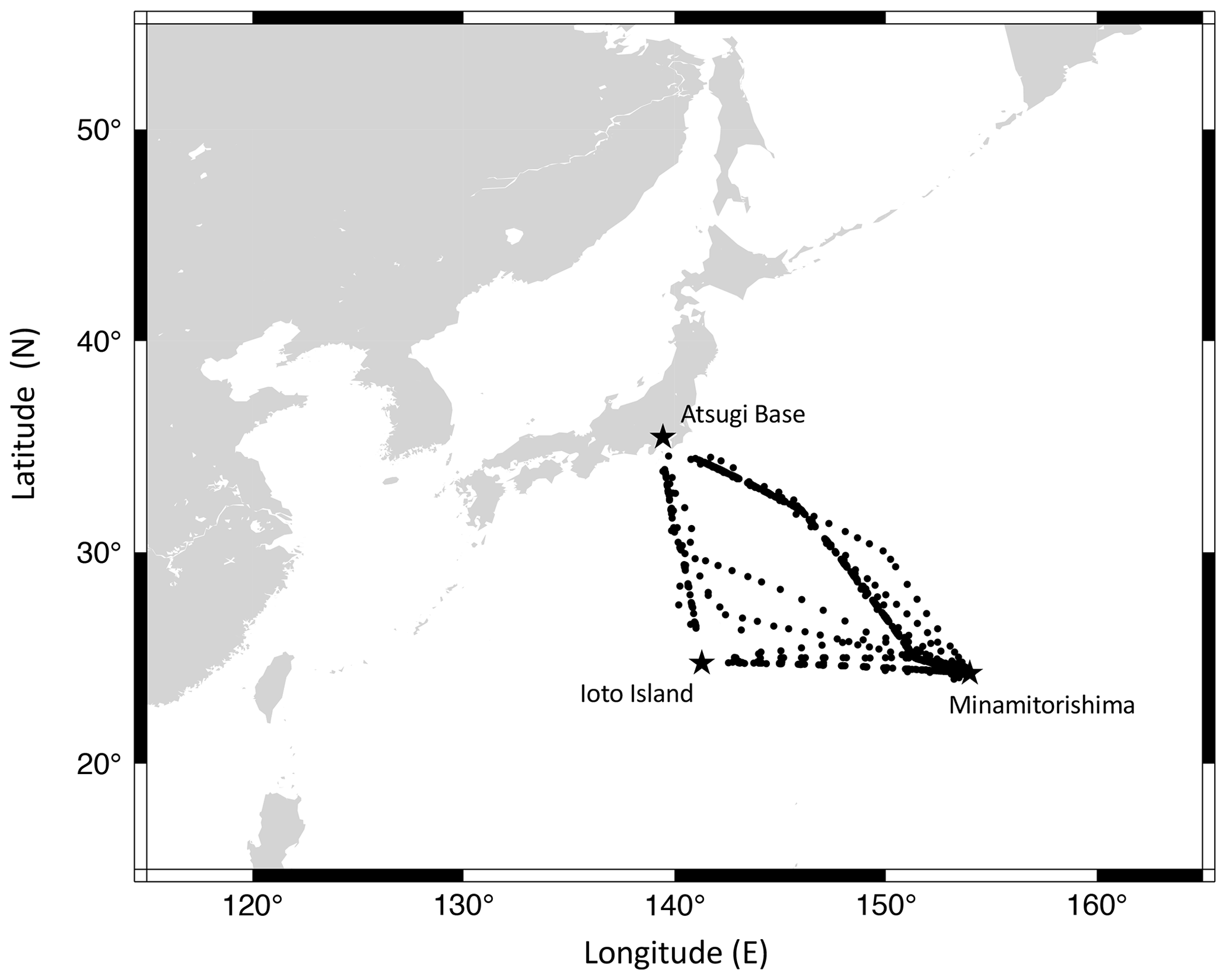
Figure 1Locations of C-130 aircraft air sampling for the period May 2012–March 2020 (circles). Locations of Minamitorishima (MNM), Ioto Island and Atsugi Base are also shown by stars. Latitudinal and vertical distributions are taken during the level flight and descent portion at MNM, respectively. In total, 2206 of air samples were collected, and 1783 of them were analyzed for and ratios, as well as the stable isotopic ratios of N2, O2 and Ar.
The flask air samples were brought back to the Japan Meteorological Agency (JMA) and analyzed for CO2, CH4, CO and N2O amount fractions. The observational results are reported by Niwa et al. (2014). The CO2 amount fraction was measured using a non-dispersive infrared analyzer (Licor, LI-7000) with a precision of better than ±0.07 µmol mol−1 (Tsuboi et al., 2013) against the World Meteorological Organization (WMO) mole fraction scales for CO2 (Zhao and Tans, 2006). The dataset is posted on the WMO's World Data Centre for Greenhouse Gases (WMO/WDCGG; https://doi.org/10.50849/WDCGG_0001-8002-1001-05-02-9999; Saito, 2016, updated, 2022). After the JMA analyses, the flasks were sent to the National Institute of Advanced Industrial Science and Technology (AIST) to measure and ratios, as well as the stable isotopic ratios of N2, O2 and Ar (Ishidoya et al., 2014). In this study, we present the measured data obtained from the air samples collected for the period May 2012–March 2020. In Fig. 1, we show all the locations where the air samples were collected on board C-130 aircraft during the observation period and the locations of MNM, Atsugi Base and Ioto Island (24.76∘ N, 141.29∘ E), Japan.
The values of δ(O2 N2) and δ(Ar N2) and stable isotopic ratios of N2, O2 and Ar (δ(15N), δ(18O) and δ(40Ar)) are reported per meg (one per meg is equal to ):
where the subscripts “sample” and “standard” refer to the values of the sample and standard air, respectively. The values of δ(O2 N2), δ(Ar N2), δ(15N), δ(18O) and δ(40Ar) of the air samples were determined against our primary standard air (cylinder no. CRC00045) using a mass spectrometer (Thermo Scientific Delta-V) (Ishidoya and Murayama, 2014) with a respective reproducibility of about 5, 8, 1.5, 3 and 13 per meg (1σ). The scale based on the primary standard air is our original scale and called the “EMRI/AIST scale” in Aoki et al. (2021).
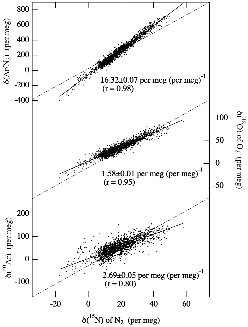
Figure 2Measured δ(Ar N2), δ(18O) of O2 and δ(40Ar) plotted against δ(15N) of N2 for all the collected air samples (solid dots). Least-squares regression lines fitted to the data are shown as solid lines, while the relationships expected from mass-dependent fractionation of air molecules are shown by dotted lines.
As already discussed in Ishidoya et al. (2014), the measured values of δ(O2 N2) are contaminated by significant artificial thermally diffusive fractionation of O2 and N2 during the air sample collection process on board the aircraft. Figure 2 shows the relationships between δ(Ar N2), δ(18O) and δ(40Ar) with δ(15N) for all the air samples analyzed in this study. It was found that δ(Ar N2), δ(18O) and δ(40Ar) change linearly in proportion to δ(15N), and the linear regression analyses gave respective slopes of (16.3±0.1), (1.58±0.01) and (2.69±0.05) per meg (per meg)−1 for the δ(Ar N2)/δ(15N), δ(18O) δ(15N) and δ(40Ar) δ(15N) ratios. These ratios agree well with the ratios of (16.2±0.1), (1.55±0.02) and (2.75±0.05) for δ(Ar N2) δ(15N), δ(18O) δ(15N) and δ(40Ar) δ(15N), respectively, determined from the laboratory experiments on the effect of thermally diffusive fractionations on δ(Ar N2), δ(15N), δ(18O) and δ(40Ar) (Ishidoya et al., 2013). Therefore, we decided to correct for the thermally diffusive fractionation of O2 and N2 on the observed δ(O2 N2) using the following equation (Ishidoya et al., 2014):
Here, δcor.(O2 N2) and δmeas.(O2 N2) denote the corrected and measured δ(O2 N2), respectively. The coefficients and are the δ(O2 N2)/δ(15N) and δ(Ar N2) δ(15N) ratios respectively, determined from the laboratory experiments as described by Ishidoya et al. (2013). The value for is not directly reported in Ishidoya et al. (2013), but it was obtained from the same laboratory experiment (Fig. 2 in their study). The ratio of is close to the Keeling et al. (2004) diffusion factor for (Ar N2) (O2 N2) and results in the same tracer δ(O2 N2)∗ (Stephens et al., 2021). Δδmeas.(Ar N2) is the deviation of the measured δ(Ar N2) from its reference point that is determined using the annual mean value of δ(Ar N2) in 2013 observed at the surface in Tsukuba (36∘ N, 140∘ E), Japan (Ishidoya and Murayama, 2014). Therefore, the effect of the seasonal δ(Ar N2) cycle on δcor.(O2 N2) was not excluded in this study. This could lead to an over- and under-correction of the surface δcor.(O2 N2) by about 2 per meg in the summertime and wintertime, respectively. Considering the measurement reproducibility of δmeas.(O2 N2) of 5 per meg, uncertainty of the correction of 2 per meg (8 per meg ; 8 per meg is the measurement reproducibility of δmeas.()) and the δ(Ar N2) seasonality, the overall uncertainty of δcor.(O2 N2) was evaluated to be less than 6 per meg. It is noted that the annual mean value of δ(Ar N2) also shows interannual variation with a peak-to-peak amplitude of 9 per meg a−1 and secular trend of 0.75 per meg a−1 (Ishidoya et al., 2021). They result in uncertainties of δcor.(O2 N2) by 2.5 and 0.1 per meg a−1 for the interannual variation and secular trend, respectively, which are significantly smaller than those of the observed δcor.(O2 N2) discussed below. The details of the correction of artificial fractionations of O2 and N2 are given in Ishidoya et al. (2014). It is noted that the correction using δ(15N), which is stable in the atmosphere over long time periods, is also suitable to obtain δcor.(O2 N2). Since the uncertainty of the corrected δcor.(O2 N2) using δ(15N) is ±7 per meg (), which is larger than that using δ(Ar N2) (±2 per meg), we determined to use δ(Ar N2) rather than δ(15N) in the present study.
We used δ(APO) for the detailed analyses of the air–sea exchange of O2. δ(APO) was calculated from the observed δcor.(O2 N2) and CO2 amount fraction:
where y(CO2) is the dry-amount fraction of CO2, αB is the OR of 1.1 for terrestrial biospheric activities, X(O2) of 0.2093–0.2094 is the amount fraction of atmospheric O2 (Tohjima et al., 2005; Aoki et al., 2019) and 2000 is an arbitrary reference. We use 0.2094 for the calculation of δ(APO). From the definition, δ(APO) is conserved for terrestrial biospheric activities and driven not only by the air–sea exchange of O2, N2 and CO2 but also by fossil fuel consumption, of which the OR value is generally larger than 1.1 (Keeling, 1988). In order to investigate the observed δcor.(O2 N2) variations, we used a three-dimensional atmospheric transport model NICAM-TM (Niwa et al., 2011) to simulate the CO2 amount fraction and δ(APO) using surface O2, N2 and CO2 fluxes. NICAM-TM is based on the Nonhydrostatic ICosahedral Atmospheric Model (NICAM; Satoh et al., 2008, 2014), and its tracer transport version has been used for atmospheric transport and flux inversion studies of greenhouse gases (e.g., Niwa et al., 2012). The horizontal model resolution used in this study had a mean grid interval of about 112 km. The model was driven by nudging the horizontal winds towards the Japanese 55-year Reanalysis data (JRA-55; Kobayashi et al., 2015).
The surface fluxes incorporated into NICAM-TM were the air–sea fluxes of O2, N2 and CO2 and also CO2 and O2 fluxes from fossil fuel combustion and the terrestrial biosphere. The air–sea O2 and N2 fluxes were the climatological seasonal anomalies taken from the TransCom experimental protocol (Blaine, 2005; Garcia and Keeling, 2001). The fluxes were computed to give the seasonal component and the annual mean values at every grid point to be zero. The air–sea CO2 flux was obtained from the monthly sea surface CO2 flux climatology of Takahashi et al. (2009). The CDIAC fossil fuel database was used for the fossil fuel CO2 flux (Andres et al., 2016; Gilfillan et al., 2019). The inversion flux reported by Niwa et al. (2012) was used for the terrestrial biosphere CO2 flux. Model-based changes in δ(APO), CO2 amount fraction and δ(O2 N2) (Δδ(APO), Δy(CO2) and Δδ(O2/N2)) were calculated using the following equations (e.g., Nevison et al., 2008; Tohjima et al., 2012) in units per meg, micromoles per mole (µmol mol−1) and per meg, respectively:
where Δy(O2), Δy(N2) and Δy(CO2) are changes in dry-amount fractions of the respective gases calculated using NICAM-TM. The superscripts “SA”, “FF”, “OC” and “TB” denote the seasonal anomaly of the air–seas O2 and N2 flux, CO2 flux from fossil fuel combustion, ocean and terrestrial biosphere, respectively. X(O2) and αB have the same meaning as in Eq. (7), while X(N2) is the dry-amount fraction of N2 in the atmosphere, and αF is the global average OR for fossil fuel combustion. In this study, we adopted X(N2)=0.7808 and αF=1.37. The αF was calculated from the fossil fuel and cement production emissions by fuel type for the period 2012–2019, reported by the Global Carbon Project (GCP; Friedlingstein et al., 2020), and the oxidative ratios for the different fuel type were taken from Keeling (1988). It should be noted that we assume initial amount fractions of y(O2) and y(N2) are equal to X(O2) and X(N2), respectively, in Eqs. (8) and (10). We can rewrite Eq. (8) as
Finally, δ(O2 N2), y(CO2) and δ(APO) obtained from NICAM-TM are reported as respective deviations of Δδ(APO), Δy(CO2) and Δδ(O2 N2) from arbitrary reference points, in other words, reported on different scales from those of observations. The δ(APO) simulation run incorporating the above-mentioned surface fluxes is referred to as the “control run”. In this calculation, δ(APO) driven by an annual mean air–sea O2 and N2 fluxes (hereafter referred to as the “δAM(APO)”), which were estimated by Gruber et al. (2001), was ignored. In other words, the δ(APO) obtained from the NICAM-TM control run ignores the contribution of not only interannual variations but also spatial distribution in annual mean air–sea O2 and N2 fluxes. If the control run represents other components other than δAM(APO) correctly, then the contribution of δAM(APO) was evaluated by subtracting the simulated δ(APO) from the observed δ(APO). In Sect. 3.2, we will discuss interannual variation in this context.
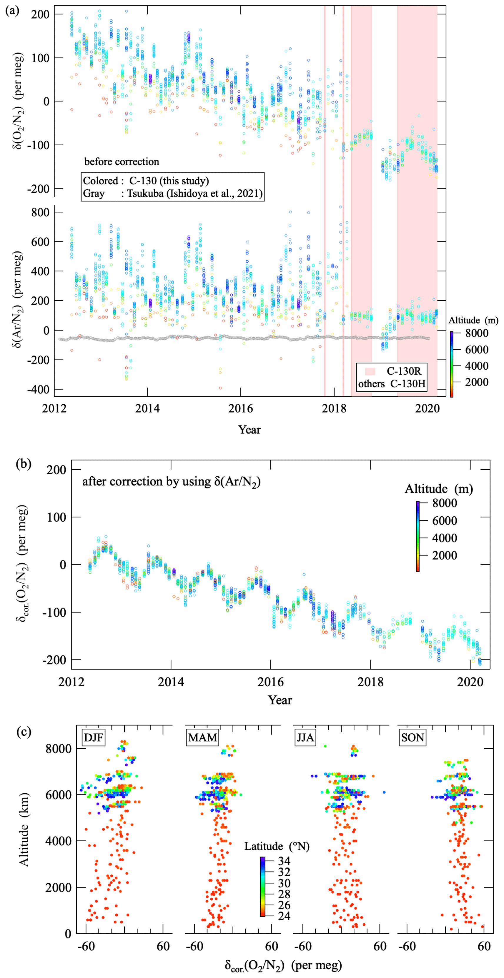
Figure 3(a) Measured values of δ(O2 N2) and δ(Ar N2) for all the air samples collected on board the C-130 aircraft. δ(Ar N2) values observed at Tsukuba, Japan, are also shown as gray circles (Ishidoya et al., 2021). Shaded areas denote the periods when C-130R aircraft was used, and C-130H aircraft was used in other periods. The color bar indicates the altitude where the air sampling was carried out. (b) δcor.(O2 N2) corrected for artificial fractionation by applying Eq. (6) (see text). The color bar indicates the altitude where the air sampling was carried out. (c) Vertical profiles of detrended δcor.(O2 N2) separated by season (DJF: December to February, MAM: March to May, JJA: June to August, and SON: September to November), obtained by subtracting a linear secular trend, fitted to the δcor.(O2 N2) in (b), from each δcor.(O2 N2) value. The color bar indicates the latitude where the air sampling was carried out.
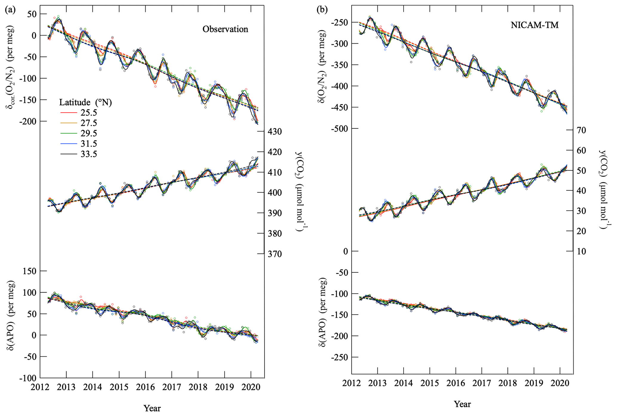
Figure 4(a) δcor.(O2 N2), CO2 amount fraction and δ(APO) observed at the altitude of (6.1±0.5) (±1σ) km at various latitudes over the western North Pacific. Best-fit curves to the data (solid lines) and secular trends (dashed lines) are also shown (Nakazawa et al., 1997a). (b) Same as in (a) but for calculated values obtained from the NICAM-TM control-run. The data from NICAM-TM are reported on arbitrary scales different from those of observations.
3.1 Latitudinal and vertical distributions of δcor.(O2 N2), CO2 amount fraction and δ(APO)
Figure 3a shows the measured δ(O2 N2) and δ(Ar N2) for all the air samples observed in this study, and Fig. 3b shows the δcor.(O2 N2) corrected values by applying Eq. (6) to the measured values. As seen from the figures, significant artificial fractionations found in the measured δ(O2 N2) are reduced dramatically by the correction. It can also be seen from Fig. 3a that the fractionations have become smaller since 2018, especially at higher altitude. It should be noted that these noted changes across 2018 could be at least partly related to changes in the aircraft type from C-130H to C-130R used for flask sampling. The periods when the C-130R was used are indicated by the pale red shade. No systematic data gaps were found in the δcor.(O2 N2) time series across 2018, so that we successfully corrected the fractionation of O2 and N2 both for C-130H and C-130R. To examine the validity of the significant corrections applied to the δmeas.(O2 N2), we also show the vertical profiles of detrended δcor.(O2 N2) separated by season in Fig. 3c, obtained by subtracting a linear secular trend from the data in Fig. 3b. As seen from the figure, seasonal δcor.(O2 N2) variations with summertime maxima are clearly seen at all altitudes, which supports validity of the correction. We also presented some examples that synoptic-scale variations in δ(O2 N2) can also be reproduced using δcor.(O2 N2) in our previous study (Fig. 4 in Ishidoya et al., 2014). Since details of the air sampling line from the inlet to flask sampler have not been informed to researchers, it is difficult to explain the cause(s) of the much lower variability in δ(Ar N2) data for periods of C-130R. The visible difference is the location of the air-conditioning blowing nozzles of C-130H and C-130R. The former and the latter are attached at the roof in the cockpit and at the front of the assistant driver's seat, respectively, and air sampling tubes are inserted into the nozzles.
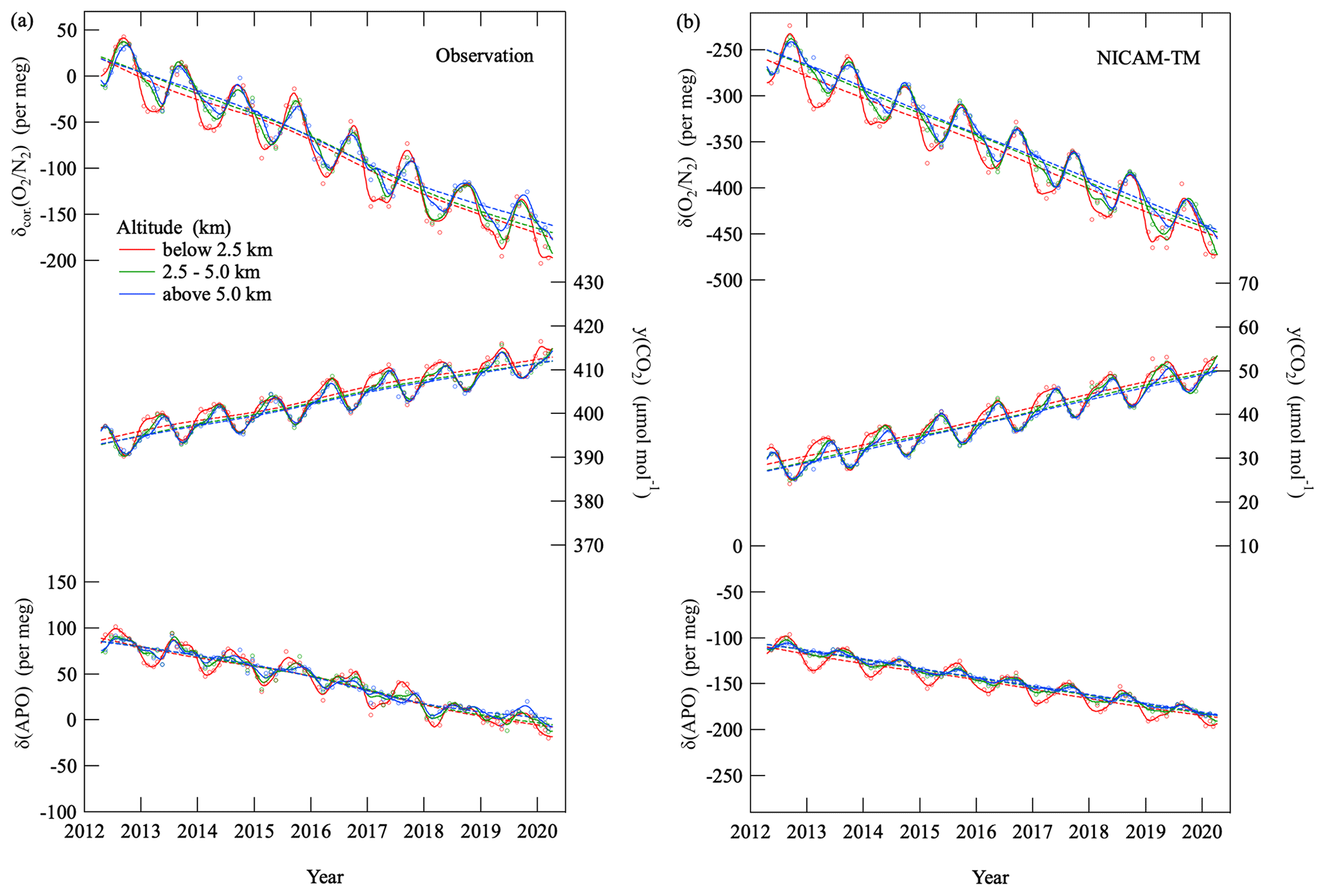
Figure 5(a) δcor.(O2 N2), the CO2 amount fraction and δ(APO) observed in the troposphere over MNM at various altitudes. Best-fit curves to the data (solid lines) and secular trends (dashed lines) are also shown (Nakazawa et al., 1997a). (b) Same as in (a) but for calculated values using NICAM-TM. The data from NICAM-TM are reported on arbitrary scales different from those of observations.
Figure 4a shows variations in the δcor.(O2 N2), CO2 amount fraction and δ(APO) observed in the layer (6.1±0.5) km (±1σ) (hereafter referred to as “middle troposphere”) at five latitudes over the western North Pacific. Best-fit curves to the data and secular trends obtained using a digital filtering technique (Nakazawa et al., 1997a) are also shown. Using this filtering technique, the average seasonal cycles were approximated by the sum of the fundamental and its first harmonic with the respective periods of 12 and 6 months. The residuals obtained by subtracting the approximated average seasonal cycle from the data were interpolated linearly to calculate daily values of δcor.(O2 N2), CO2 amount fraction and δ(APO). The daily values were smoothed by the 26th-order Butterworth filter with a cutoff period of 36 months to derive the long-term trend. The long-term trend thus obtained was subtracted from the data, and the average seasonal cycle was determined again from the residuals. These steps were repeated until an unchangeable long-term trend obtained. The observational data deviated from the best-fitted curves more than ±3σ are excluded from the analyses and not shown in the figures discussed in this study (2 % of the observational data are excluded in total). As can be seen in Fig. 4a, secular decreases in δcor.(O2 N2) and δ(APO) and increases in the CO2 amount fraction, accompanied by prominent seasonal cycles, were observed at each latitude. The secular changes in δcor.(O2 N2) and the CO2 amount fraction can be attributed mainly to O2 consumption and CO2 emission resulting from fossil fuel combustion. The seasonally dependent air–sea O2 flux and the terrestrial biospheric activity contribute towards the observed seasonal δ(O2 N2) cycle, while the terrestrial biospheric activity is the main contributor to the seasonal CO2 amount fraction cycle (e.g., Keeling et al., 1993; Keeling and Manning, 2014). The average rates of change in the observed δcor.(O2 N2), CO2 amount fraction and δ(APO) at the four latitudes shown in Fig. 4a were () per meg a−1, (2.43±0.05) and () per meg a−1, respectively, for the observational period. General features of the observed variations in δ(O2 N2), the CO2 amount fraction and δ(APO) are well reproduced by the control run of NICAM-TM, as shown in Fig. 4b. Figure 5a shows variations in δcor.(O2 N2), the CO2 amount fraction and δ(APO) observed over MNM. Clear secular trends and prominent seasonal cycles of δcor.(O2 N2), the CO2 amount fraction and δ(APO) are distinguishable, similar to those in Fig. 4a. We also note in Fig. 5a that the seasonal amplitudes of δcor.(O2 N2), the CO2 amount fraction and δ(APO) decrease with increasing altitudes. These features are also reproduced by the control run of NICAM-TM (Fig. 5b).
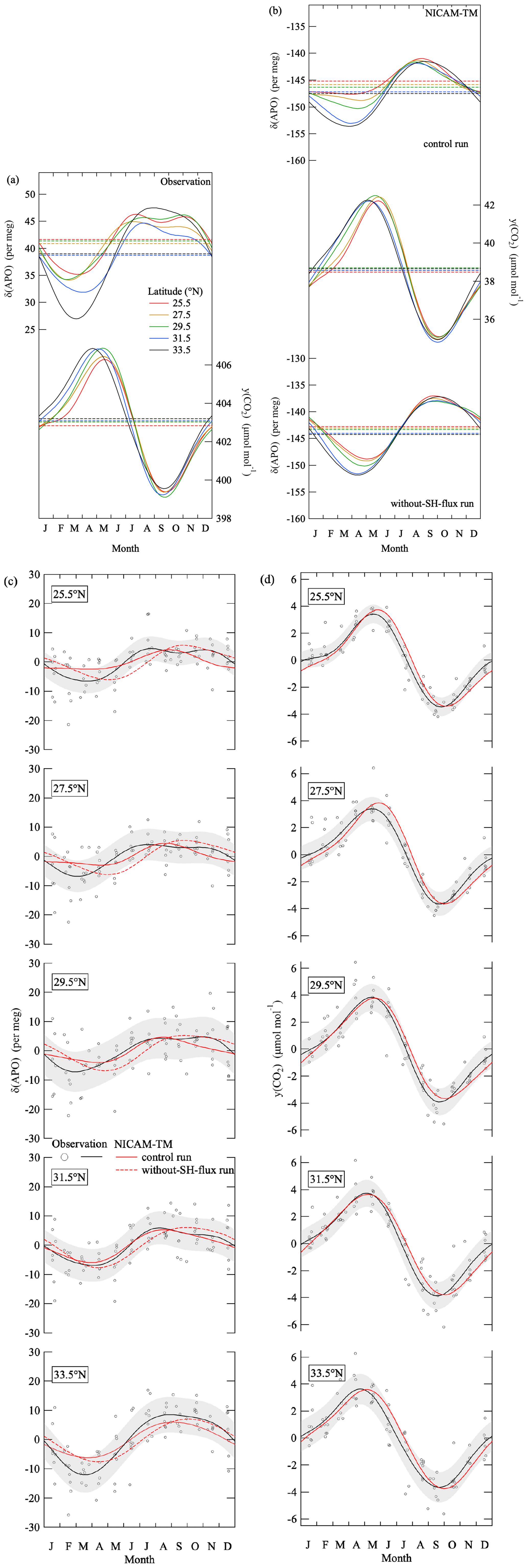
Figure 6(a) Average seasonal cycles of δ(APO) and the CO2 amount fraction observed in the troposphere at various latitudes over the western North Pacific. Dashed lines denote the average values throughout the observation period. (b) Same as in (a) but for calculated values obtained from the NICAM-TM control run and the corresponding results from the without-SH-flux run (see text). (c) Same average seasonal cycles of the observed and simulated δ(APO) in (a) and (b), along with the detrended observed values at each latitude. Error bands (shaded) indicate standard deviations of the observed δ(APO) from the average seasonal cycles (±1σ). (d) Same as in (c) but for the CO2 amount fraction.
Figure 6a shows average seasonal cycles of δ(APO) and the CO2 amount fraction observed at five latitudes over the western North Pacific. They show clear seasonal cycles with summertime maxima in δ(APO) and minima in CO2. However, the amplitude of seasonal δ(APO) cycle decreases significantly toward the lower latitudes, with seasonal maxima and minima clearly occurring earlier than those of the CO2 cycle. Figure 6b shows the corresponding average seasonal cycles of δ(APO) and the CO2 amount fraction obtained from the control run of NICAM-TM. Earlier appearances of the seasonal maxima and minima in δ(APO) than those in the CO2 amount fraction are reproduced by NICAM-TM. The seasonal amplitude of the simulated δ(APO) also decreases toward the lower latitudes, in agreement with the observation, but is underestimated. As for the CO2 amount fraction, the simulated seasonal cycles agree well with the observations. In Fig. 6c and d, we also show the same average seasonal cycles of the observed and simulated δ(APO) in Fig. 6a and b, respectively, along with the detrended observed values at each latitude for the convenience of visual comparison between the observed and simulated results.
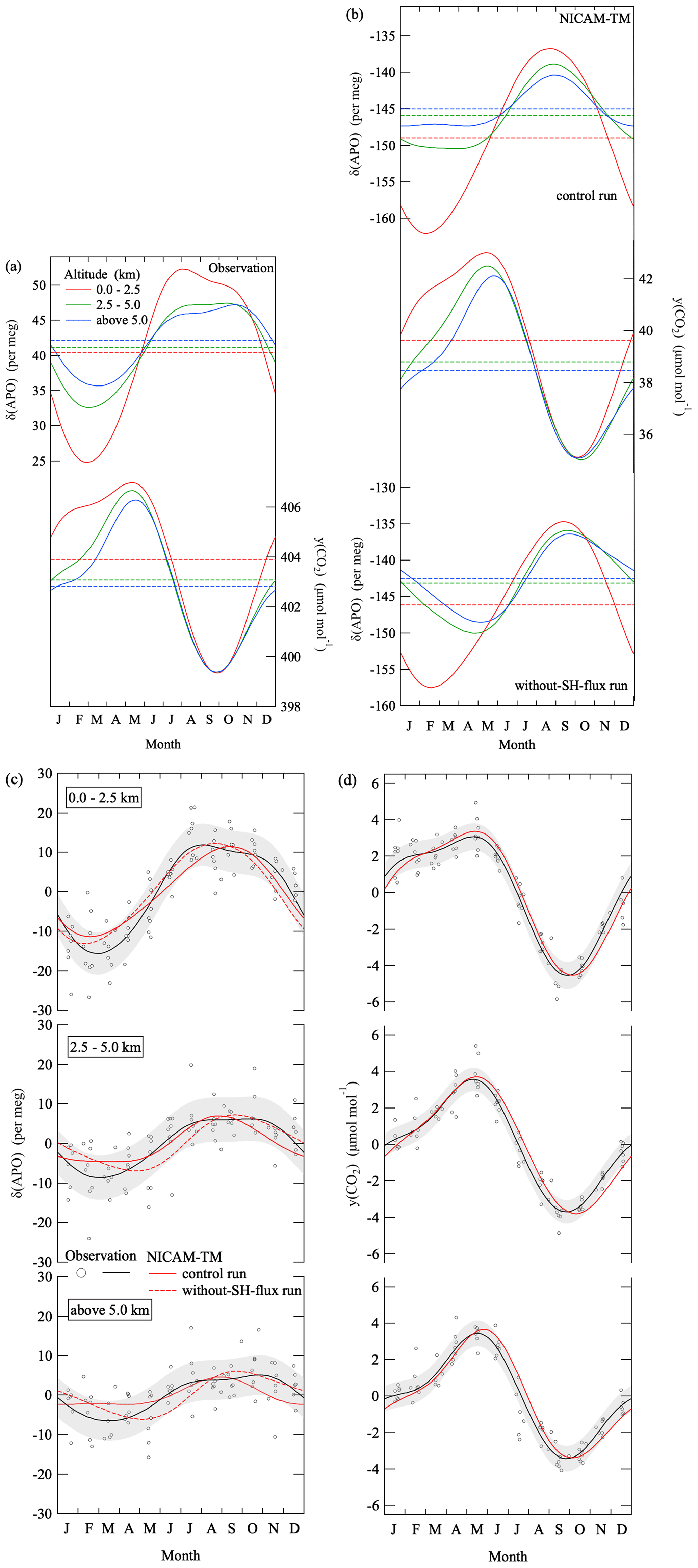
Figure 7Same as in Fig. 6 but for average seasonal cycles of δ(APO) and the CO2 amount fraction in the troposphere over MNM.
Figure 7a shows average seasonal cycles of δ(APO) and the CO2 amount fraction observed over MNM. The δ(APO) seasonal cycle varies in opposite phase to the CO2 amount fraction. However, amplitudes of the seasonal δ(APO) cycle decrease significantly with the higher altitude, with seasonal minima clearly occurring earlier than those of the CO2 cycle. These salient characteristics are reproduced generally by the NICAM-TM control run (Fig. 7b). Similar to Fig. 6, we also show Fig. 7c and d for visual comparison between the observed and simulated results.
In order to identify and explore some of the cause(s) that gave rise to the observed differences in the latitudinal and altitudinal changes in the seasonal cycles between δ(APO) and the CO2 amount fraction shown in Figs. 6a and 7a, we carried out additional NICAM-TM simulations. In the calculation, we used the same fluxes that were used in the control run but for the northern hemispheric flux only for the TransCom seasonal climatology (hereafter referred to as “without-SH-flux run”). It is well known that the opposing phase of the seasonal δ(APO) cycles between the Northern and Southern Hemisphere is due to seasonal changes in the air–sea O2 (N2) flux with summertime maxima (e.g., Keeling et al., 1998; Tohjima et al., 2012). Therefore, in comparing the control run with the without-SH-flux run, we decided to evaluate changes in the seasonal δ(APO) cycle by superimposing the anti-phase seasonal cycles through the interhemispheric mixing of air. On the other hand, the seasonal CO2 amount fraction cycle is much smaller in the Southern Hemisphere than that in the Northern Hemisphere (e.g., Nakazawa et al., 1997b). Therefore, it is expected that the seasonal cycle in the CO2 amount fraction in the Northern Hemisphere does not change significantly by the interhemispheric atmospheric mixing.

Figure 8(a) Latitudinal distribution of average ratios of the observed seasonal δ(APO) and CO2 amount fraction amplitudes calculated relative to the values observed at 25.5∘ N in the troposphere over the western North Pacific throughout the observation period (black filled circles). Error bands (shaded) indicate year-to-year variations (±1σ). The corresponding results calculated using the NICAM-TM control run (blue triangles) and the without-SH-flux run (green triangles) are also shown. Amplitude of seasonal APO cycle was calculated as a difference between an average value during July to September and that during February to April considering its broad peak, while that of CO2 amount fraction was evaluated as a difference between seasonal maximum and minimum values. (b) Same as in (a) but for vertical distribution over MNM relative to the corresponding values at 1.3 km, and amplitude of seasonal APO cycle was evaluated as a difference between an average value during July to October and that during February to April. The average fractions of surface seasonal cycles obtained from continuous observations of δ(O2 N2) and the CO2 amount fraction at MNM since December 2015 and the corresponding results calculated using NICAM-TM control run are also plotted.
The seasonal δ(APO) cycles obtained from the without-SH-flux run are also shown in Figs. 6b and 7b. As seen from Fig. 6b, latitudinal differences in the seasonal δ(APO) amplitudes from the without-SH-flux run are clearly smaller than those from the control run. In addition, appearances of the maxima and minima of the seasonal δ(APO) cycle from the without-SH-flux run are later than those from the control run, pushing the timing closer to those of seasonal CO2 amount fraction cycles. The seasonal δ(APO) cycles from the without-SH-flux run in Fig. 7b also show similar features. These results suggest that the interhemispheric mixing of air modifies the seasonal δ(APO) cycles significantly, especially in the higher altitude in the lower latitude region. To compare the observed latitudinal and altitudinal variation in the seasonal δ(APO) cycle amplitude with that calculated by NICAM-TM in more detail, Fig. 8a shows a latitudinal distribution of average fractions of the observed seasonal δ(APO) and CO2 amount fraction amplitudes relative to the 25.5∘ N values. The decrease in the seasonal amplitude of δ(APO) toward the lower latitude is about 50 %, while that of the CO2 amount fraction is less than 10 %; these are well reproduced by the control run of NICAM-TM. On the other hand, the without-SH-flux run yields a decrease in the δ(APO) amplitude by 20 % toward the lower latitude, which is significantly smaller than that from the δ(APO) from control run but slightly larger than that of the CO2 amount fraction. These results indicate that the SH makes a significant contribution to the amplitude and phase of the seasonal δ(APO) cycle at lower latitude.
Figure 8b shows average fractions of the seasonal amplitudes of δ(APO) and the CO2 amount fraction with altitude, relative to the corresponding values at 1.3 km. The average fractions of surface seasonal cycles, obtained from continuous observations of δ(O2 N2) and the CO2 amount fraction at MNM since December 2015 (updated from Ishidoya et al., 2017), are also plotted. The seasonal amplitude of δ(APO) decreases rapidly with altitude by about 70 %, while that of the CO2 amount fraction decreases by less than 20 %. The altitudinal dependence of the seasonal δ(APO) amplitude is not consistent with that of CO2. This could be attributed to the fact that the seasonal CO2 cycle is driven mainly by terrestrial biospheric activities in the northern midlatitudes and high latitudes and the seasonal minimum appears in summer, which makes the seasonal CO2 cycle uniform from the surface to the middle troposphere due to continental strong convection in summer. On the other hand, the seasonal APO cycle is driven by air–sea flux, so that altitudinal homogenization of the seasonal APO cycle due to convection is weaker than that of CO2. These features are well reproduced by the control run of NICAM-TM. The altitudinal decrease in the seasonal δ(APO) amplitude is also reproduced by the without-SH-flux run, although a slight underestimation is found above 5 km. Therefore, the altitudinal decrease in the seasonal δ(APO) amplitude over MNM is mainly due to an attenuation of the seasonal air–sea O2 and N2 fluxes around MNM with altitude, with some influence from the interhemispheric atmospheric mixing. Consequently, over the western North Pacific region, the altitude–latitude distribution of seasonal δ(APO) cycles is more sensitive to the atmospheric transport processes associated with interhemispheric air mixing and vertical attenuation of surface signal, compared with those of seasonal CO2 amount fraction cycles.
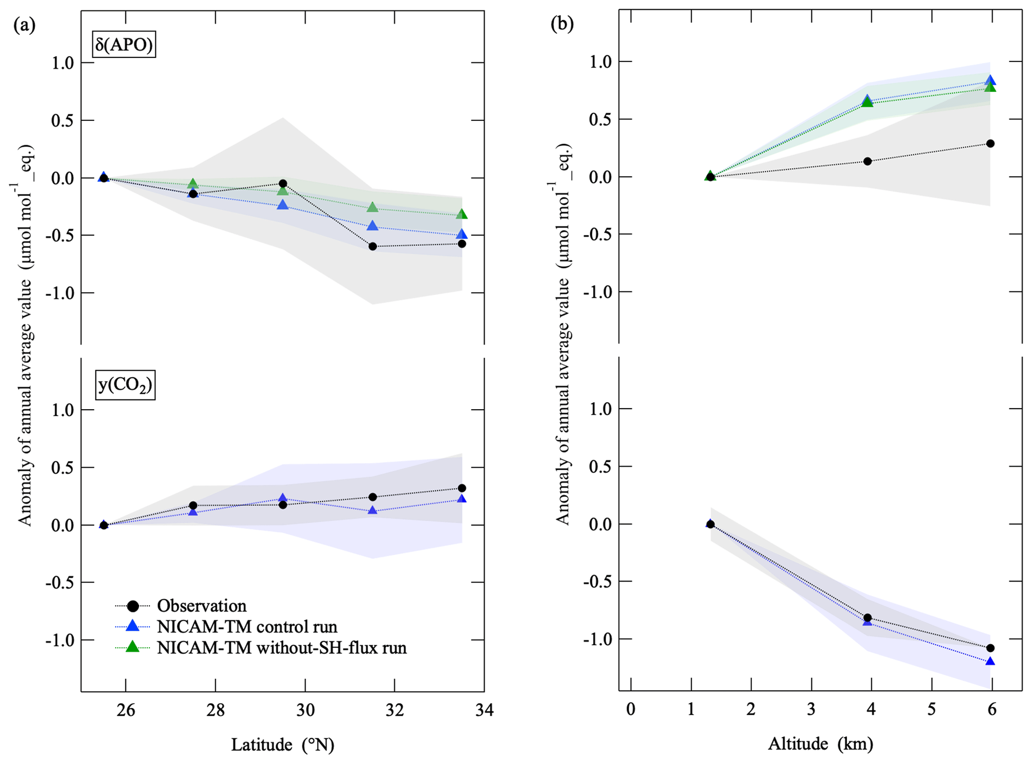
Figure 9(a) Latitudinal distribution of average deviations of the annual mean values of δ(APO) and the CO2 amount fraction relative to those at 25.5∘ N in the troposphere over the western North Pacific throughout the observation period (black filled circles). Error bands (shaded) indicate year-to-year variations (±1σ). The corresponding results calculated using NICAM-TM for the control run (blue triangles) and the without-SH-flux run (green triangles) are also shown. (b) Same as in (a) but for vertical distribution over MNM relative to the corresponding values at 1.3 km.
We also compared the observed and simulated annual mean values of δ(APO) and the CO2 amount fraction. Figure 9a shows average deviations of the middle tropospheric annual mean values of δ(APO) and the CO2 amount fraction at each latitude, relative to the 25.5∘ N values. The deviation values of δ(APO) and the CO2 amount fraction are well reproduced by the control and without-SH-flux runs. Therefore, the surface fluxes of O2, N2 and CO2 in the Northern Hemisphere are the main contributors to the observed latitudinal variations in Fig. 9a. As discussed in connection with Eq. (11), we ignored δAM(APO) in our δ(APO) simulation using NICAM-TM, which is a component of δ(APO) driven by annual mean air–sea O2 and N2 fluxes. Therefore, the results of our simulation suggest that δAM(APO) does not affect significantly the latitudinal variations in the annual mean values of the middle tropospheric δ(APO) at 25–34∘ N. Figure 9b shows the altitude deviations of the annual mean values of δ(APO) and the CO2 amount fraction, relative to their corresponding values at 1.3 km over MNM. The observed profile of the CO2 amount fraction is well reproduced by NICAM-TM. On the other hand, the average vertical gradient of δ(APO) profiles, obtained from the control and without-SH-flux runs of NICAM-TM, seems to be slightly larger than the observation. This may be due to the ignored contribution of δAM(APO); in that case, it may be that the sea area around MNM emits O2 to the atmosphere throughout the observation period. Moreover, it is clearly seen from the figure that the interannual variation in the observed δ(APO) profiles is much larger than that in the NICAM-TM simulations. This may also be due to the ignored contribution of δAM(APO), and we discuss interannual variations in the observed and simulated δ(APO) in the section below.
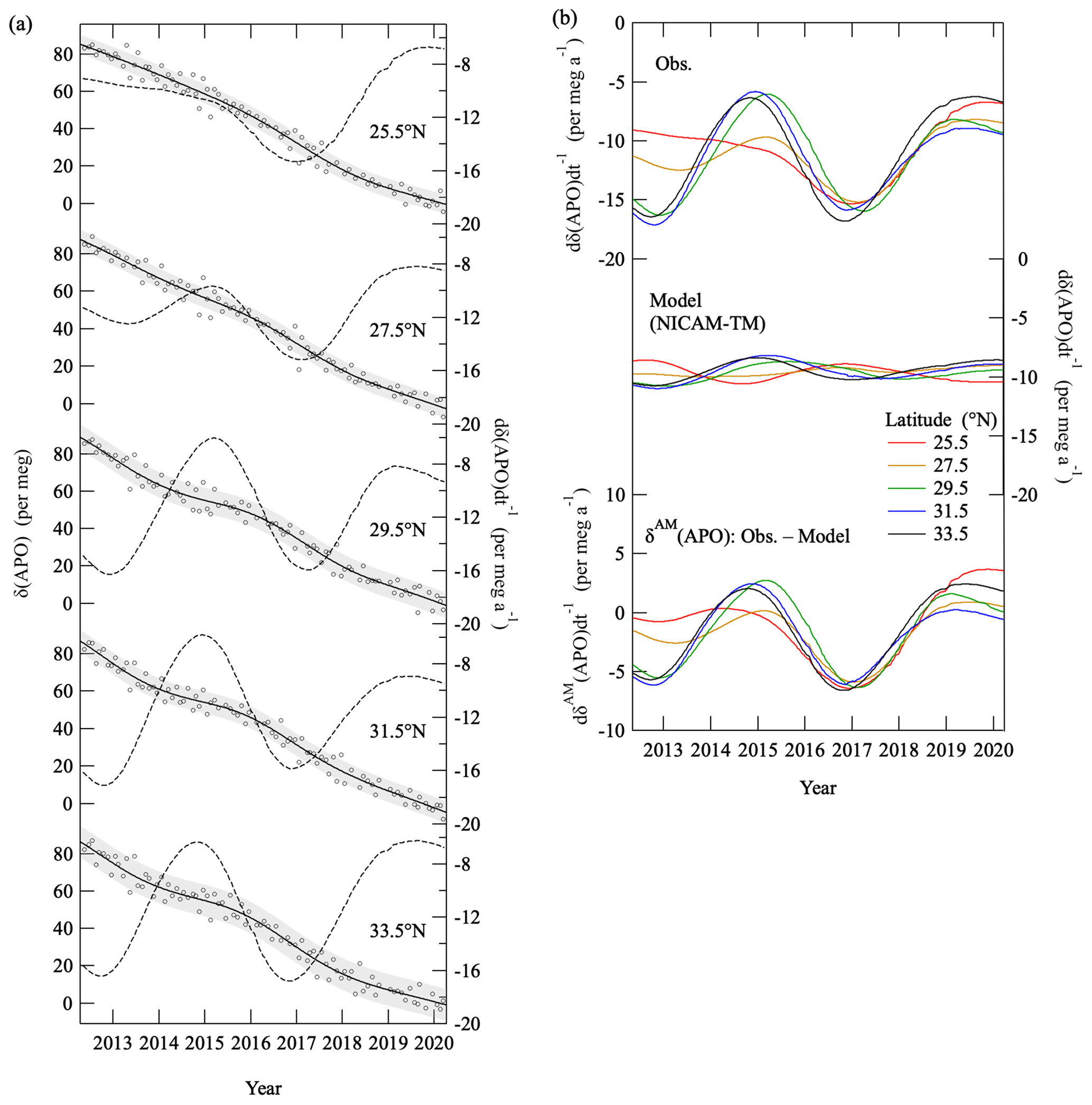
Figure 10(a) Same secular trends in Fig. 4a and their annual change rates along with the deseasonalized values of δ(APO) at each latitude over the western North Pacific. Error bands (shaded) indicate standard deviations of the deseasonalized δ (APO) from the secular trends (±1σ). (b) Same annual change rates in panel (a). The corresponding change rates for the APO obtained from the control run of NICAM-TM (middle) and those of δAM(APO) obtained by subtracting the calculated δ(APO) from the observed δ(APO) (bottom) are also shown.
3.2 Interannual variations in δ(APO) and its implication to global air–sea O2 flux and CO2 budget
In this section, we discuss causes of the interannual variations found in the middle tropospheric δ(APO) observed over the western North Pacific. Figure 10a shows the same secular trends in Fig. 4a and their annual change rates along with the deseasonalized values of δ(APO) at each latitude. The change rates observed at 29–34∘ N show interannual variation with maxima around early 2015 and mid-2019, with a minimum at all latitudes in early 2017. The corresponding change rates obtained from the control run of NICAM-TM are also shown in Fig. 10b. The change rates obtained from NICAM-TM at 29–34∘ N show interannual variations in phase with the observed rates, although the amplitudes are smaller by about 80 %. The interannual variations observed at 24–28∘ N are also larger than the simulated values. Therefore, it is likely that interannual variation in the δAM(APO), which was not incorporated into NICAM-TM, is a main contributor to the observed interannual variations at various latitudes. In this connection, it is possible that the interannual variation in the global air–sea CO2 flux could also contribute to the larger interannual variation in the observed δ(APO) since the NICAM-TM model incorporated only the monthly sea surface CO2 flux climatology to calculate δOC(APO). However, the global air–sea CO2 flux reported by the GCP (Friedlingstein et al., 2020) showed an interannual variation of 0.07 Pg a−1 during 2012–2019, corresponding to 0.2 per meg a−1 of δOC(APO), which is much smaller than the interannual variation in the observed δ(APO) shown in Fig. 10.
By assuming that all other components besides δAM(APO) are well represented in the NICAM-TM control run, we subtracted the change rates simulated by NICAM-TM from the observed rates, to extract the interannual variations due only to the δAM(APO). The calculated change rates of δAM(APO) are shown at the bottom of Fig. 10b. The change rates show similar interannual variations to the observed rates, but the latitudinal differences are smaller. This suggests that the interannual variations driven by δAM(APO) do not differ significantly as a function of latitude. In the following discussion, we make a bold assumption that an average of the change rates of δAM(APO) shown in Fig. 10b is a global average.
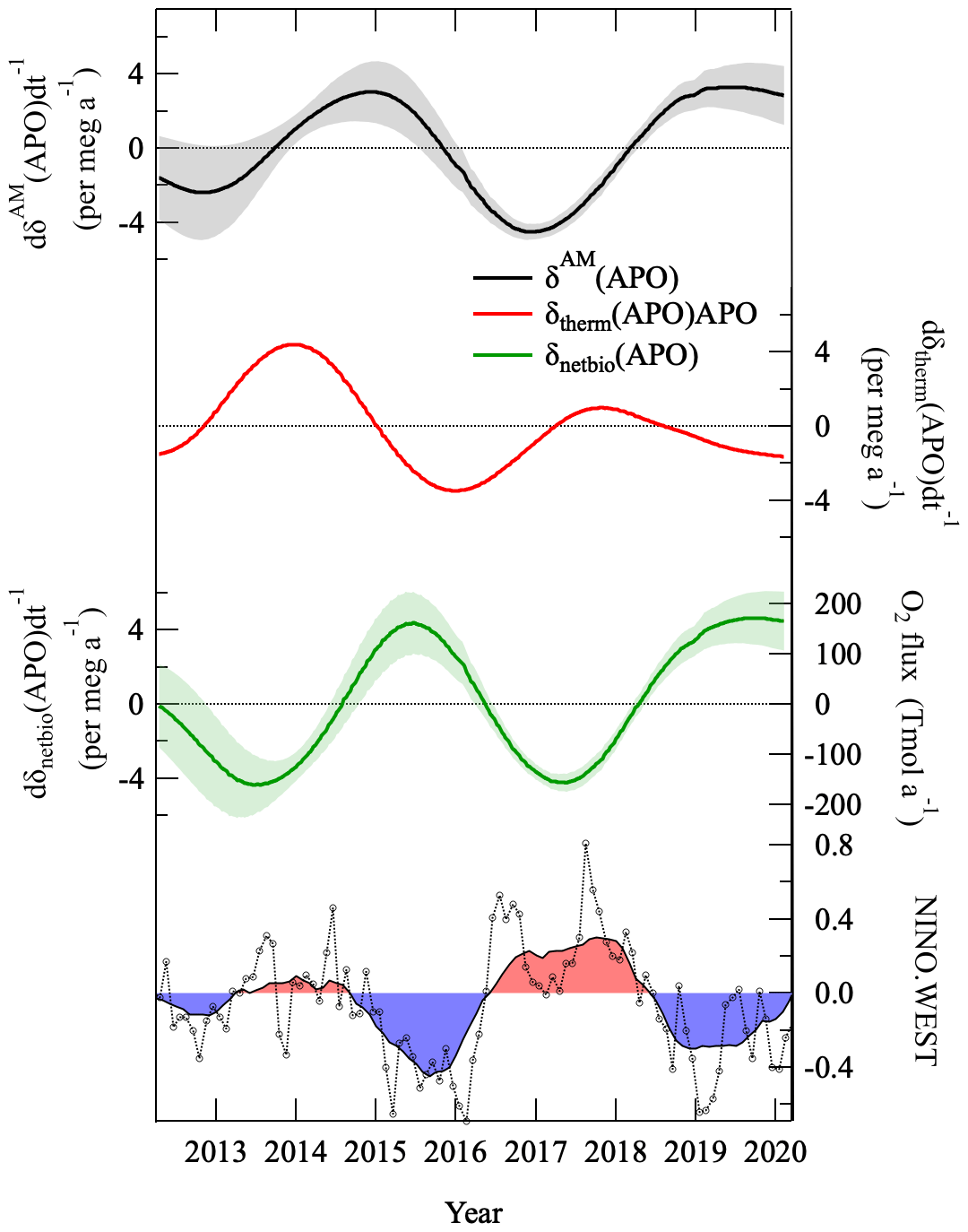
Figure 11Anomaly in the average annual change rate of δAM(APO) shown at the bottom of Fig. 10 (thick black line). Anomaly in the change rate of APO driven only by the solubility change, expected from the observed surface δ() at Tsukuba, Japan (δtherm(APO); red line, see text), and that driven by the net marine biospheric activities (δnetbio(APO); green line), obtained by subtracting the change rate of δtherm(APO) from that of δAM(APO), are shown. Anomaly in the global air–sea O2 flux corresponding to the change rate of δnetbio(APO) is also shown (see text). The time series of the NINO.WEST index (black open circles) and the annual average values of the index (thin black line) are shown at the bottom of the figure.
An anomaly of the average interannual variation of δAM(APO) change rate is shown in Fig. 11 (black line). In this figure, we also plotted a similar anomaly of interannual variation of the δ(APO) change rate due to solubility change (red line, hereafter referred to as “δtherm(APO)”). The δtherm(APO) was calculated from the δ(Ar N2) measurements observed at Tsukuba (36∘ N, 140∘ E), Japan (Ishidoya et al., 2021), by multiplying a coefficient of about 0.9 derived from differences in the solubility in O2 and Ar (Weiss, 1970). It should be noted that this is a rough approximation of the δtherm(APO), which is a combination of air–sea fluxes of O2, N2 and CO2 caused by solubility changes. As discussed in Ishidoya et al. (2021), the interannual variation in the δ(Ar N2) change rate is in phase with the global ocean heat content reported by ocean temperature measurements (e.g., Levitus et al., 2012). This suggests that δtherm(APO) is also driven by changes in the solubility of the global seawater. By subtracting δtherm(APO) from δAM(APO), we estimated interannual variation of the δ(APO) change rate due to marine biological activities (green line, hereafter referred to as “δnetbio(APO)”). It is expected that δnetbio(APO) is driven by marine biological activities, not only in the surface mixed layer but also through a ventilation of subsurface low-O2 waters.
Both the δtherm(APO) and δnetbio(APO) show significant interannual variations, roughly in opposite phase with each other. Moreover, the change rate of δnetbio(APO) varies in opposite phase with the NINO.WEST (Japan Meteorological Agency; https://www.data.jma.go.jp/gmd/cpd/db/elnino/index/ninowidx.html, last access: 13 May 2020), which is an index of the El Niño–Southern Oscillation (ENSO). The ENSO is in the El Niño and La Niña phase, respectively, during the period with the negative and positive NINO.WEST index. Therefore, the δnetbio(APO) tends to increase and decrease during El Niño and La Niña, respectively. This is consistent with Eddebbar et al. (2017), who examined global and tropical air–sea O2 flux responses to ENSO, based on the Community Earth System Model (CESM). They reported that the upper ocean loses O2 to the atmosphere during El Niño and gains O2 during La Niña, mainly due to changes in ventilation of low-O2 waters in the tropical Pacific, the region that has a dominant influence over the interannual variation in global air–sea O2 flux (McKinley et al., 2003). By assuming the interannual variation in the δnetbio(APO) represents a global average, and assuming a one-box atmosphere with 5.124×10²¹ g for the total mass of dry air (Trenberth, 1981), 28.97 g mol−1 for the mean molecular weight of dry air, and respective fractions of 0.2093 and 0.7808 for O2 and N2 in the atmosphere, we estimated an interannual variation in the global air–sea O2 flux due to marine biological activities (right axis of the green line in Fig. 11). The peak-to-peak amplitude of the O2 flux is found to be about 300 Tmol a−1, which is almost consistent with that of global APO flux estimated using the δ(APO) data from Scripps stations (Keeling and Manning, 2014) and a global atmospheric transport inversion (Rödenbeck et al., 2008; Eddebbar et al., 2017). Therefore, the seasonal cycles and interannual variations obtained from δcor.(O2 N2) have a coherent signal we can explain, although we recognize the number of simplifying assumptions is extensive to derive δnetbio(APO), and the aircraft observations are from a comparatively small region. This helps to prove that the δcor.(O2 N2) is of good quality, despite the significant correction for enormous sampling artifacts.
By assuming the average secular trends of the middle tropospheric δcor.(O2 N2) and the CO2 amount fraction observed in this study to be global average values, we were able to estimate the global CO2 budget. The equations for separating out the global net terrestrial biospheric and oceanic CO2 uptake are given by Keeling and Shertz (1992) firstly as
and
Here, B, F and O (in Pg a−1, C equivalents) are the global terrestrial biospheric CO2 uptake, the anthropogenic CO2 emitted from fossil fuel combustion and cement manufacturing, and the oceanic CO2 exchange, respectively; dδ(O2 N2)dt−1 (per meg a−1) and dy(CO2)dt−1 () are the observed change rates in atmospheric δcor.(O2 N2) and the CO2 amount fraction, respectively; 0.471 converts CO2 emissions of 1 Pg (C equivalents) to micromoles per mole of atmospheric CO2; X(O2) is the standard mole fraction of O2 in air (0.2094), αF and αB are the OR for global average fossil fuel combustion and net terrestrial biospheric activities, respectively; and Zeff (Pg a−1) represents the net effect of oceanic O2 outgassing on the oceanic and terrestrial biospheric CO2 uptakes, which has been considered since Bender et al. (2005) and Manning and Keeling (2006). As described in the “Methods” section, we use αF of 1.37 calculated from the fossil fuel and cement production emissions by fuel type reported by the GCP.
Long-term change in Zeff is caused mainly by stratification of the ocean and the decrease of O2 solubility in seawater due to a secular increase in the global ocean heat content (e.g., Bopp et al., 2002). However, as discussed above for Fig. 11, the ocean O2 outgassing shows significant interannual variation, which makes it difficult to estimate year-to-year variations in the global CO2 budget from Eqs. (12) and (13). In this regard, Tohjima et al. (2019) estimated the terrestrial biospheric and the oceanic CO2 uptakes using their δ(O2 N2) and CO2 amount fraction data, by changing the time period to obtain average secular change rates. They reported that the CO2 uptakes estimated using the change rates averaged over a longer period greater than 5 years were consistent with those reported by the GCP (Le Queéreé et al., 2018) within ±0.5 Pg a−1, while those estimated using annual change rates scattered significantly.
It seems that the averaging period needed to reduce the interannual variations in δtherm(APO) and δnetbio(APO) in Fig. 11 is about 4–5 years, similar to Nevison et al. (2008) and Tohjima et al. (2019). Therefore, we estimated average terrestrial biospheric and oceanic CO2 uptake throughout the observation period (2012–2019, 8 years) to reduce the interannual variation in Zeff sufficiently. Using the global ocean (0–2000 m) heat content data from the National Oceanographic Data Center (NOAA)/National Centers for Environmental Information (NCEI) (updated from Levitus et al., 2012, https://www.nodc.noaa.gov/OC5/3M_HEAT_CONTENT/, last access: 14 January 2020) and the same ratio of air–sea O2 (N2) flux to air–sea heat flux used in Manning and Keeling (2006), we adopted (0.6±0.6) Pg a−1 for Zeff for the period 2012–2019. We assumed 100 % uncertainty for Zeff following Manning and Keeling (2006). The value of F, (9.7±0.5) Pg a−1, was obtained from emissions from fossil fuel combustion and industrial processes by the GCP (Friedlingstein et al., 2020). Using the average secular trends of δcor.(O2 N2) and the CO2 amount fraction for the observational period of the present study, the respective terrestrial biospheric and oceanic CO2 uptakes were estimated to be (1.8±0.9) and (2.8±0.6) Pg a−1 for the period 2012–2019. These values agree well with the corresponding CO2 uptake of (1.8±1.1) and (2.6±0.5) Pg a−1 reported by the GCP (Friedlingstein et al., 2020). It is noted that the terrestrial biospheric CO2 uptake by the GCP is calculated by subtracting the CO2 emission due to land-use change ((1.6±0.7) Pg a−1) from their estimated total land CO2 uptake ((3.4±0.9) Pg a−1).
Regular air samples were taken on C-130 cargo aircraft flights from Atsugi Base to MNM, and air samples have been collected during the level flight and during the descent portion at MNM. In this paper, we have presented the analytical results of the air samples for the CO2 amount fraction, δ(O2 N2), δ(Ar N2), δ(15N) of N2, δ(18O) of O2 and δ(40Ar) for the period May 2012–March 2020. The relationships of δ(Ar N2), δ(18O) and δ(40Ar) with δ(15N) indicate a significant artificial fractionation due to thermal diffusion during the air sample collection.
The δcor.(O2/N2) values, corrected for the artificial fractionation using δ(Ar N2), and the δ(APO) values derived from δcor.(O2 N2) were shown to have clear seasonal cycles nearly in opposite phase to the cycle of the CO2 amount fraction from the surface to 6 km along the latitudinal path from 25.5 to 33.5∘ N. We then used a three-dimensional atmospheric transport model NICAM-TM that was driven by the air–sea fluxes of O2, N2 and CO2, along with fluxes of CO2 and O2 from fossil fuel combustion, to interpret some of the characteristic features we observed in the seasonal cycles and vertical profiles of APO and the CO2 amount fraction.
Seasonal amplitudes of δ(APO) and the CO2 amount fraction decreased toward the lower latitude from 34.5 to 24.5∘ N by about 50 % and less than 10 %, respectively: these features were reproduced by the corresponding ratios from the control run of NICAM-TM. On the other hand, the without-SH-flux run underestimated the latitudinal change in the δ(APO) amplitude, which indicated that the seasonal cycle of the mid-tropospheric δ(APO) was modified significantly by a combination of the northern and southern hemispheric seasonal cycles through the interhemispheric atmospheric mixing. The decrease in the δ(APO) seasonal amplitude was about 70 % with altitude from the surface to 6 km, while that of the CO2 amount fraction was less than 20 %. These features were also reproduced well by the control run of NICAM-TM.
The observed decrease in the annual mean values of the CO2 amount fraction with altitude was reproduced by the control run of NICAM-TM. On the other hand, the average vertical gradient of the δ(APO) profiles was slightly overestimated by the NICAM-TM simulations, while the simulated interannual variation was underestimated. This may be due to the ignored contribution of δAM(APO), which is a component of δ(APO) driven by annual mean air–sea O2 and N2 fluxes.
The interannual variations in the middle tropospheric δAM(APO) were estimated by subtracting the simulated δ(APO) by the NICAM-TM control run from the observed δ(APO). We also estimated the solubility-driven component of δ(APO) (δtherm(APO)) from the δ(Ar N2) observed at Tsukuba, assuming its interannual variation was driven by changes in the globally averaged solubility of the seawater. The interannual variation in δ(APO) driven by marine biological activities (δnetbio(APO)) was calculated by subtracting δtherm(APO) from δAM(APO). The δnetbio(APO) showed significant interannual variations in the opposite phase to that of δtherm(APO), and the change rate varied in opposite phase with the NINO.WEST. Therefore, the δnetbio(APO) values obtained in this study tended to increase and decrease with El Niño and La Niña, respectively, which is in agreement with Eddebbar et al. (2017), who examined responses of the global and tropical air–sea O2 flux to ENSO based on the CESM.
By assuming the observed secular trends of the middle tropospheric δcor.(O2 N2) and CO2 amount fraction to be representative of global average values, we estimated terrestrial biospheric and oceanic CO2 uptakes to be (1.8±0.9) and (2.8±0.6) Pg a−1, respectively, for the period 2012–2019. These values agree well with the corresponding CO2 uptake values of (1.8±1.1) (land) and (2.6±0.5) Pg a−1 (ocean) reported by the GCP.
Additionally, our study has shown that our aircraft observation and the method we used to correct artificial fractionation of O2 and N2 are useful in evaluating interhemispheric air mixing processes based on the seasonal δ(APO) cycle, as well as interannual variations in the global air–sea O2 flux, and in calculating global CO2 budgets based on the long-term trends of δcor.(O2 N2) and the CO2 amount fraction.
The observational data of δcor.(O2 N2) and the CO2 amount fraction are available through the World Data Centre for Greenhouse Gases (WDCGG) at https://gaw.kishou.go.jp (last access: 22 September 2021), and the respective DOIs are https://doi.org/10.50849/WDCGG_0006-8002-7001-05-02-9999 (Ishidoya, 2021) and https://doi.org/10.50849/WDCGG_0001-8002-1001-05-02-9999 (Saito, 2016, updated 2022).
SI designed the study, carried out measurements of δ(O2 N2), δ(Ar N2), δ(15N), δ(18O) and δ(40Ar), and drafted the manuscript. KT and KS managed the collections, and YN carried out the simulations of NICAM-TM using the supercomputer system (NEC SX-Aurora TSUBASA) of the National Institute for Environmental Studies (NIES). HM, SM and KI examined the results and provided feedback on the manuscript. All the authors approved the final paper.
The contact author has declared that neither they nor their co-authors have any competing interests.
Publisher's note: Copernicus Publications remains neutral with regard to jurisdictional claims in published maps and institutional affiliations.
The authors gratefully acknowledge many staff members of the Japan Ministry of Defense and Japan Meteorological Agency for supporting the long-term observations.
This study was partly supported by the JSPS KAKENHI (grant nos. 15H02814 and 19H01975) and the Global Environment Research Coordination System from the Ministry of the Environment, Japan (grant nos. METI1454 and METI1953).
This paper was edited by Jan Kaiser and reviewed by three anonymous referees.
Andres, R. J., Boden, T., and Marland, G.: Monthly Fossil-Fuel CO2 Emissions: Mass of Emissions Gridded by One Degree Latitude by One Degree Longitude, Carbon Dioxide Information Analysis Center, Oak Ridge National Laboratory, U.S. Department of Energy, Oak Ridge, Tenn., USA, https://doi.org/10.3334/CDIAC/ffe.MonthlyMass.2016, 2016.
Aoki, N., Ishidoya, S., Matsumoto, N., Watanabe, T., Shimosaka, T., and Murayama, S.: Preparation of primary standard mixtures for atmospheric oxygen measurements with less than 1 µmol mol−1 uncertainty for oxygen molar fractions, Atmos. Meas. Tech., 12, 2631–2646, https://doi.org/10.5194/amt-12-2631-2019, 2019.
Aoki, N., Ishidoya, S., Tohjima, Y., Morimoto, S., Keeling, R. F., Cox, A., Takebayashi, S., and Murayama, S.: Intercomparison of ratio scales among AIST, NIES, TU, and SIO based on a round-robin exercise using gravimetric standard mixtures, Atmos. Meas. Tech., 14, 6181–6193, https://doi.org/10.5194/amt-14-6181-2021, 2021.
Bender, M. L., Ho, D. T., Hendricks, M. B., Mika, R., Battle, M., and co-authors.: Atmospheric changes, 1993–2002: Implications for the partitioning of fossil fuel CO2 sequestration, Global Biogeochem. Cycles., 19, GB4017, https://doi.org/10.1029/2004GB002410, 2005.
Bent, J.: Airborne Oxygen Measurements over the Southern Ocean as an Integrated Constraint of Seasonal Biogeochemical Processes, UC San Diego, ProQuest ID: Bent_ucsd_0033D_14471, Merritt ID: ark:/20775/bb1059815c, https://escholarship.org/uc/item/4dd6k6j2 (last access: 15 May 2022), 2014.
Birner, B., Chipperfield, M. P., Morgan, E. J., Stephens, B. B., Linz, M., Feng, W., Wilson, C., Bent, J. D., Wofsy, S. C., Severinghaus, J., and Keeling, R. F.: Gravitational separation of and age of air in the lowermost stratosphere in airborne observations and a chemical transport model, Atmos. Chem. Phys., 20, 12391–12408, https://doi.org/10.5194/acp-20-12391-2020, 2020.
Blaine, T. W.: Continuous measurements of atmospheric argon/nitrogen as a tracer of air-sea heat flux : models, methods, and data. UC San Diego, ProQuest ID: umi-ucsd-1040, Merritt ID: ark:/20775/bb21509964, https://escholarship.org/uc/item/9bn929w7 (last access: 15 May 2022), 2005.
Bopp, L., Le Quéré, C., Heimann, M., Manning, A. C., and Monfray, P.: Climate-induced oceanic oxygen fluxes: implications for the contemporary carbon budget, Global Biogeochem. Cy., 16, 1022, https://doi.org/10.1029/2001GB001445, 2002.
Cohen, E. R., Cvitas, T., Frey, J. G., Holmstrom, B., Kuchitsu, K., Marquardt, R., Mills, I., Pavese, F., Quack, M., Stohner, J., Strauss, H., Takami, M., and Thor, A. J.: IUPAC Green Book: 3rd edn., RSC Publishing, ISBN 0854044337, ISBN-13 9780854044337, 2007.
Eddebbar, Y. A., Long, M. C., Resplandy, L., Rödenbeck, C., Rodgers, K. B., Manizza, M., and Keeling, R. F.: Im- pacts of ENSO on air-sea oxygen exchange: Observations and mechanisms, Global Biogeochem. Cy., 31, 901–921, https://doi.org/10.1002/2017GB005630, 2017.
Friedlingstein, P., O'Sullivan, M., Jones, M. W., Andrew, R. M., Hauck, J., Olsen, A., Peters, G. P., Peters, W., Pongratz, J., Sitch, S., Le Quéré, C., Canadell, J. G., Ciais, P., Jackson, R. B., Alin, S., Aragão, L. E. O. C., Arneth, A., Arora, V., Bates, N. R., Becker, M., Benoit-Cattin, A., Bittig, H. C., Bopp, L., Bultan, S., Chandra, N., Chevallier, F., Chini, L. P., Evans, W., Florentie, L., Forster, P. M., Gasser, T., Gehlen, M., Gilfillan, D., Gkritzalis, T., Gregor, L., Gruber, N., Harris, I., Hartung, K., Haverd, V., Houghton, R. A., Ilyina, T., Jain, A. K., Joetzjer, E., Kadono, K., Kato, E., Kitidis, V., Korsbakken, J. I., Landschützer, P., Lefèvre, N., Lenton, A., Lienert, S., Liu, Z., Lombardozzi, D., Marland, G., Metzl, N., Munro, D. R., Nabel, J. E. M. S., Nakaoka, S.-I., Niwa, Y., O'Brien, K., Ono, T., Palmer, P. I., Pierrot, D., Poulter, B., Resplandy, L., Robertson, E., Rödenbeck, C., Schwinger, J., Séférian, R., Skjelvan, I., Smith, A. J. P., Sutton, A. J., Tanhua, T., Tans, P. P., Tian, H., Tilbrook, B., van der Werf, G., Vuichard, N., Walker, A. P., Wanninkhof, R., Watson, A. J., Willis, D., Wiltshire, A. J., Yuan, W., Yue, X., and Zaehle, S.: Global Carbon Budget 2020, Earth Syst. Sci. Data, 12, 3269–3340, https://doi.org/10.5194/essd-12-3269-2020, 2020.
Garcia, H. and Keeling, R.: On the global oxygen anomaly and air-sea flux, J. Geophys. Res., 106, 31155–31166, 2001.
Gilfillan, D., Marland, G., Boden, T., and Andres, R.: Global, Regional, and National Fossil-Fuel CO2 Emissions, Carbon Dioxide Information Analysis Center at Appalachian State University, Boone North Carolina, https://energy.appstate.edu/CDIAC (last access: 21 July 2020), 2019.
Goto, D., Morimoto, S., Ishidoya, S., Aoki, S., and Nakazawa, T.: Terrestrial biospheric and oceanic CO2 uptake estimated from long-term measurements of atmospheric CO2 mole fraction, δ13C and δ(O2 N2) at Ny-Ålesund, Svalbard, J. Geophys. Res.-Biogeosci., 122, 1192–1202, https://doi.org/10.1002/2017JG003845, 2017.
Gruber, N., Gloor, M., Fan, S.-M., and Sarmiento, J.: Air-sea flux of oxygen estimated from bulk data: Implications for the marine and atmospheric oxygen cycles, Global Biogeochem. Cy., 15, 783–803, 2001.
Ishidoya, S.: Atmospheric ratio by Aircraft (Western North Pacific), ver. 2021-09-16-1302, National Institute of Advanced Industrial Science and Technology [data set], https://doi.org/10.50849/WDCGG_0006-8002-7001-05-02-9999, 2021.
Ishidoya, S. and Murayama, S.: Development of high precision continuous measuring system of the atmospheric and ratios and its application to the observation in Tsukuba, Japan, Tellus B, 66, 22574, https://doi.org/10.3402/tellusb.v66.22574, 2014.
Ishidoya, S., Morimoto, S., Sugawara, S., Watai, T., Machida, T., Aoki, S., Nakazawa, T., and Yamanouchi, T.: Gravitational separation suggested by , δ15N of N2, δ18O of O2, observed in the lowermost part of the stratosphere at northern middle and high latitudes in the early spring of 2002, Geophys. Res. Lett., 35, L03812, https://doi.org/10.1029/2007GL031526, 2008.
Ishidoya, S., Aoki, S., Goto, D., Nakazawa, T., Taguchi, S., and Patra, P. K.: Time and space variations of the ratio in the troposphere over Japan and estimation of global CO2 budget, Tellus B, 64, 18964, https://doi.org/10.3402/tellusb.v64i0.18964, 2012.
Ishidoya, S., Sugawara, S., Morimoto, S., Aoki, S., Nakazawa, T., Honda, H., and Murayama, S.: Gravitational separation in the stratosphere – a new indicator of atmospheric circulation, Atmos. Chem. Phys., 13, 8787–8796, https://doi.org/10.5194/acp-13-8787-2013, 2013.
Ishidoya, S., Tsuboi, K., Matsueda, H., Murayama, S., Taguchi, S., Sawa, Y., Niwa, Y., Saito, K., Tsuji, K., Nishi, H., Y. Baba, Y., Takatsuji, S., Dehara, K., and Fujiwara, H.: New atmospheric ratio measurements over the western North Pacific using a cargo aircraft C-130H, SOLA, 10, 23–28, https://doi.org/10.2151/sola.2014-006, 2014.
Ishidoya, S., Tsuboi, K., Murayama, S., Matsueda, H., Aoki, N., Shimosaka, T., Kondo, H., and Saito, K.: Development of a continuous measurement system for atmospheric ratio using a paramagnetic analyzer and its application in Minamitorishima Island, Japan, SOLA, 13, 230–234, 2017.
Ishidoya, S., Sugawara, S., Tohjima, Y., Goto, D., Ishijima, K., Niwa, Y., Aoki, N., and Murayama, S.: Secular change in atmospheric and its implications for ocean heat uptake and Brewer–Dobson circulation, Atmos. Chem. Phys., 21, 1357–1373, https://doi.org/10.5194/acp-21-1357-2021, 2021.
Kawamura, K., Severinghaus, J., Ishidoya, S., Sugawara, S., Hashida, G., Motoyama, H., Fujii, Y., Aoki, S., and Nakazawa, T.: Convective mixing of air in firn at four polar sites, Earth Planet. Sc. Lett., 244, 672–682, 2006.
Keeling, R. F.: Development of an interferometric oxygen analyzer for precise measurement of the atmospheric O2 mole fraction, PhD thesis, Harvard University, USA, 1988.
Keeling, R. F. and Manning, A. C.: Studies of recent changes in atmospheric O2 content, in Treatise on Geochemistry, 2nd edn., Elsevier, Amsterdam, 5, 385–404, 2014.
Keeling, R. F. and Shertz, S. R.: Seasonal and interannual variations in atmospheric oxygen and implications for the global carbon cycle, Nature, 358, 723–727, 1992.
Keeling, R. F., Bender, M. L., and Tans, P. P.: What atmospheric oxygen measurements can tell us about the global carbon cycle, Global Biogeochem. Cycles, 7, 37–67, 1993.
Keeling, R. F., Stephens, B. B., Najjar, R. G., Doney, S. C., Archer, D., and Heimann, M.: Seasonal variations in the atmospheric ratio in relation to the kinetics of air-sea gas exchange, Global Biogeochem. Cycles, 12, 141–163, 1998.
Keeling, R. F., Blaine, T., Paplawsky, B., Katz, L., Atwood, C., and Brockwell, T.: Measurement of changes in atmospheric ratio using a rapid-switching, single-capillary mass spectrometer system, Tellus B, 56, 322–338, https://doi.org/10.3402/tellusb.v56i4.16453, 2004.
Kobayashi, S., Ota, Y., Harada, Y., Ebita, A., Moriya, M., On- oda, H., Onogi, K., Kamahori, H., Kobayashi, C., Endo, H., Miyaoka, K., and Takahashi, K.: The JRA-55 Reanalysis: general specifications and basic characteristics, J. Meteorol. Soc. Jpn., 93, 5–48, https://doi.org/10.2151/jmsj.2015-001, 2015.
Le Quéré, C., Andrew, R. M., Friedlingstein, P., Sitch, S., Hauck, J., Pongratz, J., Pickers, P. A., Korsbakken, J. I., Peters, G. P., Canadell, J. G., Arneth, A., Arora, V. K., Barbero, L., Bastos, A., Bopp, L., Chevallier, F., Chini, L. P., Ciais, P., Doney, S. C., Gkritzalis, T., Goll, D. S., Harris, I., Haverd, V., Hoffman, F. M., Hoppema, M., Houghton, R. A., Hurtt, G., Ilyina, T., Jain, A. K., Johannessen, T., Jones, C. D., Kato, E., Keeling, R. F., Goldewijk, K. K., Landschützer, P., Lefèvre, N., Lienert, S., Liu, Z., Lombardozzi, D., Metzl, N., Munro, D. R., Nabel, J. E. M. S., Nakaoka, S., Neill, C., Olsen, A., Ono, T., Patra, P., Peregon, A., Peters, W., Peylin, P., Pfeil, B., Pierrot, D., Poulter, B., Rehder, G., Resplandy, L., Robertson, E., Rocher, M., Rödenbeck, C., Schuster, U., Schwinger, J., Séférian, R., Skjelvan, I., Steinhoff, T., Sutton, A., Tans, P. P., Tian, H., Tilbrook, B., Tubiello, F. N., van der Laan-Luijkx, I. T., van der Werf, G. R., Viovy, N., Walker, A. P., Wiltshire, A. J., Wright, R., Zaehle, S., and Zheng, B.: Global Carbon Budget 2018, Earth Syst. Sci. Data, 10, 2141–2194, https://doi.org/10.5194/essd-10-2141-2018, 2018.
Levitus, S., Antonov, J. I., Boyer, T. P., Baranova, O. K., Garcia, H. E., Locarnini, R. A., Mishonov, A. V., Reagan, J. R., Seidov, D., Yarosh, E. S., and Zweng, M. M.: World ocean heat content and thermosteric sea level change (0–2000 m), 1955–2010, Geophys. Res. Lett., 39, L10603, https://doi.org/10.1029/2012GL051106, 2012.
Manning, A. C. and Keeling, R. F.: Global oceanic and terrestrial biospheric carbon sinks from the Scripps atmospheric oxygen flask sampling network, Tellus B, 58, 95–116, 2006.
McKinley, G. A., Follows, M. J, Marchall, J., and Fan, S.-M.: Inter- annual variability of air-sea O2 fluxes and the determination of CO2 sinks using atmospheric , Geophys. Res. Lett., 30, 1101, https://doi.org/10.1029/2002GL016044, 2003.
Morgan, E. J., Stephens, B. B., Long, M. C., Keeling, R. F., Bent, J. D., McKain, K., Sweeney, C., Hoecker- Marti?nez, M. S., and Kort, E. A.: Summertime Atmo- spheric Boundary Layer Gradients of O2 and CO2 over the Southern Ocean, J. Geophys. Res., 124, 13439–13456, https://doi.org/10.1029/2019JD031479, 2019.
Nakazawa, T., Ishizawa, M., Higuchi, K., and Trivett, N. B. A.: Two curve fitting methods applied to CO2 flask data, Environmetrics, 8, 197–218, 1997a.
Nakazawa, T., Morimoto, S., Aoki, S., and Tanaka, M.: Temporal and spatial variations of the carbon isotopic ratio of atmospheric carbon dioxide in the western Pacific region, J. Geophys. Res., 102, 1271–1285, 1997b.
Nevison, C. D., Mahowald, N. M., Doney, S. C., Lima, I. D., and Cassar, N.: Impact of variable air-sea O2 and CO2 fluxes on atmospheric potential oxygen (APO) and land-ocean carbon sink partitioning, Biogeosciences, 5, 875–889, https://doi.org/10.5194/bg-5-875-2008, 2008.
Nevison, C. D., Keeling, R. F., Kahru, M., Manizza, M., Mitchell, B. G., and Cassar N.: Estimating net community production in the Southern ocean based on atmospheric potential oxygen and satellite ocean color data, Glob. Biogeochem. Cycles., 26, GB1020, https://doi.org/10.1029/2011GB004040, 2012.
Niwa, Y., Tomita, H., Satoh, M., and Imasu, R.: A Three-Dimensional Icosahedral Grid Advection Scheme Preserving Monotonicity and Consistency with Continuity for Atmospheric Tracer Transport, J. Meteorol. Soc. Jpn., 89, 255–268, https://doi.org/10.2151/jmsj.2011-306, 2011.
Niwa, Y., Machida, T., Sawa, Y., Matsueda, H., Schuck, T. J., Brenninkmeijer, C. A. M., Imasu, R., and Satoh, M.: Imposing strong constraints on tropical terrestrial CO2 fluxes using passenger aircraft based measurements, J. Geophys. Res., 117, D11303, https://doi.org/10.1029/2012JD017474, 2012.
Niwa, Y., Tsuboi, K., Matsueda, H., Sawa, Y., Machida, T., Nakamura, M., Kawasato, T., Saito, K., Takatsuji, S., Tsuji, K., Nishi, H., Dehara, K., Baba, Y., Kuboike, D., Iwatsubo, S., Ohmori, H., and Hanamiya, Y.: Seasonal Variations of CO2, CH4, N2O and CO in the Mid-troposphere over the Western North Pacific Observed using a C-130H Cargo Aircraft, J. Meteorol. Soc. Japan, 92, 55–70, https://doi.org/10.2151/jmsj.2014-104, 2014.
Rödenbeck, C., Le Quéré, C., Heimann, M., and Keeling, R. F.: Interannual variability inoceanic biogeochemical pro- cesses inferred by inversion of atmospheric and CO2 data, Tellus B, 60, 685–705, https://doi.org/10.1111/j.1600-0889.2008.00375.x, 2008.
Saito, K.: Atmospheric CO2 by Aircraft (Western North Pacific), Japan Meteorological Agency [data set], https://doi.org/10.50849/WDCGG_0001-8002-1001-05-02-9999, 2016, updated 2022.
Satoh, M., Matsuno, T., Tomita, H., Miura, H., Nasuno, T., and Iga, S.: Nonhydrostatic icosahedral atmospheric model (NICAM) for global cloud resolving simulations, J. Comput. Phys., 227, 3486–3514, https://doi.org/10.1016/j.jcp.2007.02.006, 2008.
Satoh, M., Tomita, H., Yashiro, H., Miura, H., Kodama, C., Seiki, T., Noda, A. T., Yamada, Y., Goto, D., Sawada, M., Miyoshi, T., Niwa, Y., Hara, M., Ohno, T., Iga, S., Arakawa, T., Inoue, T., and Kubokawa, H.: The Non-hydrostatic Icosahedral Atmospheric Model: description and development, Progress in Earth and Planetary Science, 1, 1–32, https://doi.org/10.1186/s40645-014-0018-1, 2014.
Severinghaus, J.: Studies of the terrestrial O2 and carbon cycles in sand dune gases and in biosphere 2, PhD thesis, Columbia University, New York, 1995.
Steinbach, J.: Enhancing the usability of atmospheric oxygen measurements through emission source characterization and airborne measurement, PhD thesis, Friedrich-Schiller-Universität, 2010.
Stephens, B. B., Keeling, R. F., Heimann, M., Six, K. D., Murnane, R., and Caldeira, K.: Testing global ocean carbon cycle models using measurements of atmospheric O2 and CO2 concentration, Global Biogeochem. Cycles, 12, 213–230, 1998.
Stephens, B. B., Keeling, R. F., and Paplawsky, W. J.: Shipboard measurements of atmospheric oxygen using a vacuum-ultraviolet absorption technique, Tellus B, 55, 857–878, 2003.
Stephens, B. B., Long, M. C., Keeling, R. F., Kort, E. A., Sweeney, C., Apel, E. C., Atlas, E. L., Beaton, S., Bent, J. D., Blake, N. J., Bresch, J. F., Casey, J., Daube, B. C., Diao, M. H., Diaz, E., Dierssen, H., Donets, V., Gao, B. C., Gierach, M., Green, R., Haag, J., Hayman, M., Hills, A. J., Hoecker-Martinez, M. S., Honomichl, S. B., Hornbrook, R. S., Jensen, J. B., Li, R. R., McCubbin, I., McKain, K., Morgan, E. J., Nolte, S., Powers, J. G., Rainwater, B., Randolph, K., Reeves, M., Schauffler, S. M., Smith, K., Smith, M., Stith, J., Stossmeister, G., Toohey, D. W., and Watt, A. S.: The Ratio and CO2 Airborne Southern Ocean Study, B. Am. Meteor. Soc., 99, 381–402, https://doi.org/10.1175/bams-d-16-0206.1, 2018.
Stephens, B. B., Morgan, E. J., Bent, J. D., Keeling, R. F., Watt, A. S., Shertz, S. R., and Daube, B. C.: Airborne measurements of oxygen concentration from the surface to the lower stratosphere and pole to pole, Atmos. Meas. Tech., 14, 2543–2574, https://doi.org/10.5194/amt-14-2543-2021, 2021.
Sturm, P., Leuenberger, M., Moncrieff, J., and Ramonet, M.: Atmospheric O2, CO2 and δ13C measurements from aircraft sampling over Griffin Forest, Perthshire, UK, Rapid Commun. Mass Spectrom., 19, 2399–2406, https://doi.org/10.1002/rcm.2071, 2005.
Takahashi, T., Sutherland, S. C., Wanninkhof, R., Sweeney, C., Feely, R. A., Chipman, D. W., Hales, B., Friederich, G., Chavez, F., Sabine, C., Watson, A., Bakker, D. C. E., Schuster, U., Metzl, N., Yoshikawa-Inoue, H., Ishii, M., Midorikawa, T., Nojiri, Y., Körtzinger, A., Steinhoff, T., Hoppema, M., Olafsson, J., Arnar- son, T. S., Tilbrook, B., Johannessen, T., Olsen, A., Bellerby, R., Wong, C. S., Delille, B., Bates, N. R., and de Baar H. J. W.: Climatological mean and decadal change in surface ocean pCO2, and net sea-air CO2 flux over the global oceans, Deep-Sea Res. Pt. II, 56, 554–577, https://doi.org/10.1016/j.dsr2.2008.12.009, 2009.
Tohjima, Y., Machida, T., Watai, T., Akama, I., Amari, T., and Moriwaki, Y.: Preparation of gravimetric standards for measurements of atmospheric oxygen and reevaluation of atmospheric oxygen concentration, J. Geophys. Res., 110, D1130, https://doi.org/10.1029/2004JD005595, 2005.
Tohjima, Y., Mukai, H., Nojiri, Y., Yamagishi, H., and Machida, T.: Atmospheric measurements at two Japanese sites: estimation of global oceanic and land biotic carbon sinks and analysis of the variations in atmospheric potential oxygen (APO), Tellus B, 60, 213–225, 2008.
Tohjima, Y., Minejima, C., Mukai, H., Machida, T., Yamagishi, H., and Nojiri, Y.: Analysis of seasonality and annual mean distribution of atmospheric potential oxygen (APO) in the Pacific region, Glob. Biogeochem. Cy., 26, GB4008, https://doi.org/10.1029/2011GB004110, 2012.
Tohjima, Y., Mukai, H., Machida, T., Hoshina, Y., and Nakaoka, S.-I.: Global carbon budgets estimated from atmospheric and CO2 observations in the western Pacific region over a 15-year period, Atmos. Chem. Phys., 19, 9269–9285, https://doi.org/10.5194/acp-19-9269-2019, 2019.
Trenberth, K. E.: Seasonal variations in global sea level pressure and the total mass of the atmosphere, J. Geophys. Res., 86, 5238–5246, 1981.
Tsuboi, K., Matsueda, H., Sawa, Y., Niwa, Y., Nakamura, M., Kuboike, D., Saito, K., Ohmori, H., Iwatsubo, S., Nishi, H., Hanamiya, Y., Tsuji, K., and Baba, Y.: Evaluation of a new JMA aircraft flask sampling system and laboratory trace gas analysis system, Atmos. Meas. Tech., 6, 1257–1270, https://doi.org/10.5194/amt-6-1257-2013, 2013.
Van der Laan, S., van der Laan-Luijk, I. T., Rödenbeck, C., Varlagin, A., Shironya, I., Neubert, R. E. M., and Ramonet, M.: Atmospheric CO2, δ(O2 N2), APO and oxidative ratios from aircraft flask samples over Fyodorovskoye, Western Russia, Atmos. Environ., 97, 174–181, 2014.
Weiss, R. F.: The solubility of nitrogen, oxygen and argon in water and seawater, Deep-Sea Res., 17, 721–735, 1970.
Wofsy, S. C., Daube, B., Jimenez, R., Kort, E., Pittman, J. V., Park, S., Commane, R., Xiang, B., Santoni, G., Jacob, D., Fisher, J., Pickett-Heaps, C., Wang, H., Wecht, K. J., Wang, Q.-Q., Stephens, B. B., Shertz, S., Romashkin, P., Campos, T., Haggerty, J., Cooper, W. A., Rogers, D., Beaton, S., Hendershot, R., Elkins, J. W., Fahey, D., Gao, R., Moore, F., Montzka, S. A., Schwarz, J., Hurst, D., Miller, B., Sweeney, C., Oltmans, S., Nance, D., Hintsa, E., Dutton, G., Watts, L., Spackman, R., Rosenlof, K., Ray, E., Zondlo, M. A., Diao, M., Keeling, R., Bent, J., Atlas, E., Lueb, R., Mahoney, M. J., Chahine, M., Olson, E., Patra, P., Ishijima, K., Engelen, R., Flemming, J., Nassar, R., Jones, D. B. A., and Fletcher, S. E. M.: HIAPER Pole-to-Pole Observations (HIPPO): fine grained, global-scale measurements of climatically important atmospheric gases and aerosols, Philos. T. Roy. Soc. A, 369, 2073–2086, https://doi.org/10.1098/rsta.2010.0313, 2011.
Zhao, C. L. and Tans, P. P.: Estimating uncertainty of the WMO mole fraction scale for carbon dioxide in air, J. Geophys. Res., 111, D08S09, https://doi.org/10.1029/2005JD006003, 2006.