the Creative Commons Attribution 4.0 License.
the Creative Commons Attribution 4.0 License.
 | 30 May 2022
Towards reconstructing the Arctic atmospheric methane history over the 20th century: measurement and modelling results for the North Greenland Ice Core Project firn
Satoshi Sugawara
Kenji Kawamura
Ikumi Oyabu
Stephen J. Andrews
Takuya Saito
Shuji Aoki
Takakiyo Nakazawa
Systematic measurements of atmospheric methane (CH4) mole fractions at the northern high latitudes only began in the early 1980s. Although CH4 measurements from Greenland ice cores consistently covered the period before ∼ 1900, no reliable observational record is available for the intermediate period. We newly report a data set of trace gases from the air trapped in firn (an intermediate stage between snow and glacial ice formation) collected at the NGRIP (North Greenland Ice Core Project) site in 2001. We also use a set of published firn air data at the NEEM (North Greenland Eemian ice Drilling) site. The two Arctic firn air data sets are analysed with a firn air transport model, which translates historical variations to depth profiles of trace gases in firn. We examine a variety of possible firn diffusivity profiles, using a suite of measured trace gases, and reconstruct the CH4 mole fraction by an iterative dating method. Although the reconstructions of the Arctic CH4 mole fraction before the mid-1970s still has large uncertainties (> 30 ppb – parts per billion), we find a relatively narrow range of atmospheric CH4 history that is consistent with both depth profiles of NGRIP and NEEM. The atmospheric CH4 history inferred by this study is more consistent with the atmospheric CH4 scenario prepared for the NEEM firn modelling than that for the CMIP6 (Climate Model Intercomparison Project Phase 6) experiments. Our study shows that the atmospheric CH4 scenario used for the NEEM firn modelling is considered to be the current best choice for the Arctic CH4 history, but it should not be used to tune firn air transport models until being verified by further measurements from sources such as the Arctic ice cores. Given the current difficulty in reconstructing the CH4 history with low uncertainty from the firn air data sets from Greenland, future sampling and measurements of ice cores at a high-accumulation site may be the only way to accurately reconstruct the atmospheric CH4 trend over the 20th century.
- Article
(7857 KB) - Full-text XML
- BibTeX
- EndNote


Methane (CH4) is an important atmospheric greenhouse gas emitted from both natural and anthropogenic sources. Despite making great efforts to understand its global budget, emission estimates of individual sources still have large quantitative uncertainties (e.g. Saunois et al., 2020; Chandra et al., 2021). Anthropogenic activities have enhanced CH4 emissions globally and more than doubled the abundance of atmospheric CH4 over the industrial era (e.g. Etheridge et al., 1998). The CH4 emission histories have been estimated based on human activity statistics combined with emission factors (Stern and Kaufmann, 1996; van Aardenne et al., 2001). Such historical emission inventories have been examined by atmospheric chemistry transport modelling (Houweling et al., 2000; Monteil et al., 2011; Ghosh et al., 2015), in combination with the records of atmospheric CH4 mole fraction reconstructed from polar ice cores (Blunier et al., 1993; Nakazawa et al., 1993; Etheridge et al., 1998; MacFarling Meure et al., 2006; Sapart et al., 2012) and air extracted from porous snow layers at the top of ice sheets (firn; Francey et al., 1999; Buizert et al., 2012; Sapart et al., 2013).
A large fraction of natural and anthropogenic CH4 sources resides in the Northern Hemisphere, and thus, the atmospheric CH4 trend of the Northern Hemisphere can provide important information on the evolution of anthropogenic CH4 emissions and the variations in natural CH4 emission in response to climatic variability. The interhemispheric gradient of CH4 mole fraction is also key to the allocation of CH4 emissions between both hemispheres (e.g. Dlugokencky et al., 2003; Ghosh et al., 2015; Chandra et al., 2021).

Figure 1Atmospheric CH4 mole fraction data covering the last 300 years. Symbols in brown are from the Southern Hemisphere; crosses and open circles are from the Law Dome ice core and firn, respectively (Etheridge et al., 1998; MacFarling Meure et al., 2006; Rubino et al., 2019). Open squares are from Kennaook / Cape Grim (CGO; MacFarling Meure et al., 2006), and dots are from the South Pole (SPO; ftp://aftp.cmdl.noaa.gov/, last access: 10 December 2021). Other coloured data (except for yellow) are from the Northern Hemisphere. Closed green squares, triangles, and diamonds are from the EUROCORE (Blunier et al., 1993), EUROCORE and GISP2 (Etheridge et al., 1998), and Site J (Nakazawa et al., 1993) ice cores. Red dots are the NEEM-S1 ice core (Rhodes et al., 2013), blue dots are from Alert, Canada (ALT), and Barrow, Alaska (BRW; ftp://aftp.cmdl.noaa.gov/), and light blue and yellow lines are the atmospheric scenarios prepared for the NEEM firn modelling (Buizert et al., 2012) and the CMIP6 experiments (Meinshausen et al., 2017), respectively. For the latter, Arctic and Antarctic scenarios with higher and lower mole fractions are shown, respectively.
Systematic measurements of atmospheric CH4 mole fraction began in the 1980s. In Fig. 1, CH4 measurements at two Arctic sites, i.e. Barrow, Alaska (BRW), and Alert, Canada (ALT), whose records start in 1983 and 1985, respectively, are shown (blue dots; data provided by National Oceanic and Atmospheric Administration/Earth System Research Laboratory/Global Monitoring Laboratory, NOAA/ESRL/GML). Although some sparse data from the 1970s are available (e.g. Rice et al., 2016), such direct measurements provide CH4 data only from around 1980, which means that some reconstruction methodology is required to infer atmospheric CH4 mole fraction variations before that time. For this purpose, air extracted from ice cores and firn layers has been measured. Figure 1 also presents CH4 mole fractions analysed in ice cores from Greenland (closed green symbols), such as EUROCORE (Blunier et al., 1993), EUROCORE and GISP2 (Greenland Ice Sheet Project 2; Etheridge et al., 1998), and Site J (Nakazawa et al., 1993). These data show fairly good agreement with each other until ∼ 1900, after which the number of data and the consistency among the records are poor. Continuous measurements from North Greenland Eemian Ice Drilling (NEEM)-S1 ice core (Rhodes et al., 2013) presented CH4 mole fractions before ∼ 1960 (red in Fig. 1), but their data are notably higher than other ice core data after ∼ 1850 (Blunier et al., 1993; Etheridge et al., 1998; Nakazawa et al., 1993). Therefore, the inconsistency among the different data sets indicates that the period between ∼ 1900 and ∼ 1980 is not covered reliably either by direct observations or ice core reconstructions.
In comparison to these data, higher-resolution CH4 data are available from Antarctica (brown in Fig. 1). The comprehensive Law Dome ice core and firn data set (Etheridge et al., 1998; MacFarling Meure et al., 2006; Rubino et al., 2019) almost continuously covers the last 300 years and is well connected to the direct measurements at the South Pole (SPO; data provided by NOAA/ESRL/GML) and Kennaook / Cape Grim (CGO; Etheridge et al., 1998; MacFarling Meure et al., 2006). Such consistency and continuity among the data sets suggest that the Antarctic CH4 data can serve as a good reference to represent the global atmospheric CH4 trend over the past few centuries.
Despite the limited observational data as described above, two synthetic data sets for the Arctic historical CH4 mole fractions are currently available (see Sect. 3.2 for details). Buizert et al. (2012) prepared Arctic historical trends of mole fractions of atmospheric trace gases, including CH4 (light blue in Fig. 1), which in turn was used to constrain the gas diffusivity profile in firn at the NEEM site. Considered as the most likely atmospheric CH4 trend for the northern high latitudes, this scenario was treated as a known history, by which the diffusivity profiles in firn were tuned in firn air transport models (Witrant et al., 2012; Trudinger et al., 2013). The other is the composite data set prepared for use in the CMIP6 experiments (yellow in Fig. 1; Meinshausen et al., 2017). It is seen that their scenario for the northernmost latitude (higher mole fraction; yellow line in Fig. 1) follows the NEEM-S1 ice core data set (red) and is inconsistent with the Buizert et al. (2012) scenario (light blue).
For constraining the global CH4 budget, isotope ratios of CH4 could provide useful information for relative contributions of different types of CH4 sources. Sapart et al. (2013) examined the reconstruction of stable carbon isotope ratio (δ13C) of atmospheric CH4 using firn air measurements from both the Northern and Southern hemispheres. They concluded that, with the available firn measurements and understanding of firn air transport, it is difficult to consistently reconstruct the past trend of δ13C of CH4 because of multiple reasons, including uncertainty in the atmospheric CH4 mole fraction scenario. Among many important and uncertain factors, the accurate reconstruction of the atmospheric CH4 mole fraction is particularly important because the trend in the mole fraction can lead to a significant signal in the modelled δ13C profile in firn due to the difference in the molecular diffusion coefficient, even in the absence of a temporal trend in atmospheric δ13C. Reducing the uncertainty of the historical trend of the CH4 mole fraction is therefore also important for utilising isotope data for a better understanding of the historical changes of different CH4 emission categories.
In this study, we present a set of mole fractions of CH4 and other trace gases in firn air samples collected at the NGRIP (North Greenland Ice Core Project) site. Using the available atmospheric scenarios, we simulate the depth profiles of trace gases in the NGRIP firn with our firn air transport model and those in the NEEM firn reported previously (Buizert et al., 2012). It will be shown in series of firn modelling in this study that, compared to other trace gases, CH4 is uniquely underconstrained in its Arctic history. We examine a variety of modelling cases for different diffusivity profiles and reconstruct the Arctic atmospheric CH4 over the late 20th century using an iterative dating approach (Trudinger et al., 2002). The reconstructed CH4 trends from both NGRIP and NEEM firn air samples are evaluated by comparison to the atmospheric CH4 scenarios. The uncertainty of the Arctic atmospheric CH4 history for use in firn air modelling is discussed.
Firn air was sampled at the Greenland site NGRIP (75.10∘ N, 42.32∘ W; 2959 m a.m.s.l. – above mean sea level) in May–June 2001. Mean accumulation, surface density, temperature, and pressure are 179 kg m−2 yr−1, 300 kg m−3, 241 K, and 680 hPa, respectively. Details of the firn and firn air sampling have been described elsewhere (Kawamura et al., 2006; Ishijima et al., 2007). At the NGRIP site, two shallow holes (EU and Japanese holes) were drilled (Kawamura et al., 2006; Landais et al., 2006), and the present data are from the firn air samples collected from the Japanese hole. The total number of air sampling depths is 24.
Since the technical details are reported in Kawamura et al. (2021a), only brief descriptions of the relevant data presented in this study are given here. CH4 mole fractions of the firn air samples were measured using a gas chromatograph (Agilent 6890, Agilent Technologies, Inc.) equipped with a gas chromatograph flame ionisation detector (GC-FID) at Tohoku University (TU), with a reproducibility of 2 ppb (parts per billion; Umezawa et al., 2014). The CH4 mole fractions were determined against our working standard gases that were calibrated on the TU1987 CH4 scale (Aoki et al., 1992; Umezawa et al., 2014; Fujita et al., 2018). The difference between the TU1987 CH4 scale and the WMO (World Meteorological Organization) CH4 mole fraction scale (on which the NEEM CH4 data were measured) is estimated to be ∼ 0.5 ppb at the current atmospheric CH4 levels (Fujita et al., 2018). Oyabu et al. (2020) reported that ice core data analysed on the TU1987 and WMO scales showed good agreement within analytical uncertainties, indicating consistency of both scales, including for the lower mole fractions (e.g. ∼ 700 ppb). It is therefore likely that the difference between both scales is well below the variations of interest in this study, and thus, no correction is applied for use of the NGRIP and NEEM firn data.
The firn air samples were measured for CO2 and SF6 mole fractions, respectively, by using a nondispersive infrared gas analyser (NDIR) and a gas chromatograph equipped with an electron capture detector (GC-ECD) at TU. The measurement reproducibility is estimated to be 0.02 ppm (parts per million) for CO2 and 0.09 ppt (parts per trillion) for SF6, and mole fractions of both gases are reported on the TU2010 CO2 and TU2002 SF6 scales, respectively (Sugawara et al., 2018). Although not presented in this study, the firn air samples were also previously analysed for nitrous oxide (N2O) and its isotope ratios (Ishijima et al., 2007).
As part of this study, the NGRIP firn air samples were newly analysed for selected halocarbons (CFC-11, CFC-12, CFC-113, and CH3CCl3) on the vacuum preconcentration and refocusing–gas chromatography–mass spectrometry (VPR-GCMS) system, which was developed based on the work by Saito et al. (2006). An aliquot of the sample was transferred into an evacuated canister of ∼ 0.3 L at around ambient pressure (∼ 100 kPa), and the inner pressure of the canister was recorded. The air is extracted by a vacuum pump through a preconcentration trap filled with HayeSep D cooled to −135 ∘C using a Stirling cooler. The preconcentration trap was heated to −70 ∘C to release major atmospheric constituents and then up to 100 ∘C to transfer the trapped compounds to a cryofocusing trap containing Carboxen 1000/Tenax TA at −100 ∘C. The trap was then heated to 180 ∘C to inject the trapped gases onto a PoraBOND Q separation column for subsequent analysis on MS. Mole fractions of individual halocarbons are determined against a working standard gas (compressed dry air) that was calibrated against synthetic standards on the NIES-08 (National Institute for Environmental Studies) scales.
We also use a suite of trace gas measurement data from the NEEM site (77.45∘ N, 51.06∘ W; 2450 m a.m.s.l.). The firn air samples were collected in July 2008. The details of firn air sampling and gas measurements have been described by Buizert et al. (2012). The depth profile data of all the above trace gases (CH4, CO2, SF6, CFC-11, CFC-12, CFC-113, and CH3CCl3) from the NEEM firn are used in this study together with HFC-134a and 14CO2 data that are available from NEEM but not for NGRIP.
Since the gas diffusivity in firn layers is significantly lower than in the atmosphere, the movements of atmospheric constituents are driven mostly by molecular diffusion according to their vertical mole fraction gradients under the influence of gravity. In general, lighter air components (or isotopologues) diffuse faster under their mole fraction gradients, while heavier components accumulate in the deeper layers due to the gravitational effect. Hence, the depth profiles of trace gas mole fractions in firn are determined by the atmospheric histories transferred towards depth in the firn by the molecular diffusion driven by the mole fraction gradient and gravity. At the bottom of firn, the air is trapped as bubbles in the ice sheet, which creates slow downward motion of firn air.
The firn column can be divided into the following three zones: a convective zone (CZ), a diffusive zone (DZ), and a lock-in zone (LIZ; Sowers et al., 1992; Kawamura et al., 2006; Buizert et al., 2012). In CZ, primarily driven by surface winds and fluctuations of atmospheric pressure, air is mixed with the overlying atmosphere (Sowers et al., 1992; Kawamura et al., 2006). The CZ thickness is estimated to be below 2 m at NGRIP (Kawamura et al., 2006) and 4.5 m at NEEM (Buizert et al., 2012). In DZ, which is sufficiently isolated from the surface turbulence, the movement of air is governed by molecular diffusion. Gravitational enrichment according to the barometric equation (i.e. linear increases of δ15N of N2 and δ18O of O2) occurs with depth and stops at the top of LIZ (Sowers et al., 1992; Schwander et al., 1993; Kawamura et al., 2006). The top of LIZ (lock-in depth) is at a depth of 63 m, which is coincidently the same at NGRIP (Kawamura et al., 2006) and NEEM (Buizert et al., 2012). In LIZ, advection with the enclosing ice matrix dominates the transport of air, and air parcels are gradually isolated as bubbles. Traditionally, it was supposed that high-density impermeable ice layers stop diffusivity in LIZ completely; however, recent studies demonstrated finite diffusivity in LIZ (Severinghaus et al., 2010; Buizert et al., 2012; Trudinger et al., 2013). The deepest air sampling was successfully made at 77.71 m at NGRIP (Kawamura et al., 2021a) and 77.75 m at NEEM (Buizert et al., 2012), and total pore closure is considered in the deeper layers in our modelling.
3.1 Modelling firn air transport
We use a one-dimensional diffusion model that has been used for the reconstruction of isotope ratios of CO2 and N2O (Sugawara et al., 2003; Ishijima et al., 2007). The model is conceptually similar to that developed by Trudinger et al. (1997); it is based on a theoretical formation of diffusion (Schwander et al., 1993) and a bubble-trapping process (Rommelaere et al., 1997). Air movement in the firn is driven by molecular diffusion and a gravitational effect. In other words, a trace gas flux (F) in firn is expressed by the following:
where D is the effective diffusivity of a trace gas molecule (m2 s−1), the variables s, c, and T are open porosity (unitless), trace gas molar concentration (mol m−3), and firn temperature (K), respectively, and the constants m, g, and R are the mass number of the trace gas (kg mol−1), the acceleration of gravity (m s−2), and the gas constant (J mol−1 K−1), respectively. Vertical advection flux of the trace gas, caused by air trapping at the close-off zone and downward bulk motion of firn, is expressed by using the equation given by Rommelaere et al. (1997). Conservation of the trace gas is given by the following:
for the open pore space and, in the following, by:
for bubbles. Here c and cb are trace gas molar concentrations in the open pore space and bubbles, respectively. The vertical speed of air (m yr−1) in the open pore space v is distinguished from that of firn itself vf. The vertical speed of firn vf(z) is simply given by dividing the accumulation rate by the firn density under the assumption of the steady-state densification of firn. At the transition zone where the open pore air is gradually trapped into bubbles, mass conservation is given by using a bubble-trapping rate r (s−1), which simply means that a portion of the trace gas molar concentration in the open pore space (rc) is added to bubbles. The bubble-trapping rate is given as a function of the open porosity, the total porosity, and the vertical speed of firn itself (Rommelaere et al., 1997). The total porosity was calculated from the firn density data. At the transition zone, the total porosity should be divided into the open and closed porosity. The closed porosity sc in the NGRIP firn was calculated by the empirical equation, given by Schawander (1989), as follows:
where st is the total porosity, and ρ and ρclose are the density of firn and that at the close-off depth (kg m−3), respectively. For the NEEM firn, the closed porosity sc was calculated as per Buizert et al. (2012), who followed the parameterisation by Goujon et al. (2003), as follows:
where sclose is the mean close-off porosity (9.708 × 10⁻²), according to Buizert et al. (2012).
3.2 Atmospheric scenarios
To simulate depth profiles of trace gases in firn, atmospheric histories of the target gases are required. In this study, we used atmospheric histories prepared by the NEEM firn air modelling (Buizert et al., 2012) and by the CMIP6 experiments (Meinshausen et al., 2017) for all the trace gases presented in this study for the NGRIP and NEEM firn (CH4, CO2, SF6, CFC-11, CFC-12, CFC-113, HFC-134a, CH3CCl3, and 14CO2). Since Meinshausen et al. (2017) provide latitudinally gridded data sets, their historical data for the northernmost latitude (82.5∘ N) are used. Note that the 14CO2 history for CMIP6 is available from another study (Graven et al., 2017), which is also used in this study. The 14CO2 data by Graven et al. (2017) are available in Δ14CO2 for three zonal bands (Northern Hemisphere, the tropics, and Southern Hemisphere) and were converted to 14CO2 mole fraction, as in Buizert et al. (2012). These atmospheric scenarios (hereafter referred to as the BZ and CMIP6 scenarios) are compared in Fig. 2. The BZ (light blue) and CMIP6 (blue) Arctic scenarios show compatible historical trends in many trace gases. There are, however, slight differences in some trace gases between the two scenarios, e.g. SF6 and CFC-12, but we later show that these differences do not cause significant biases in reproducing their depth profiles at the NGRIP and NEEM firn sites.
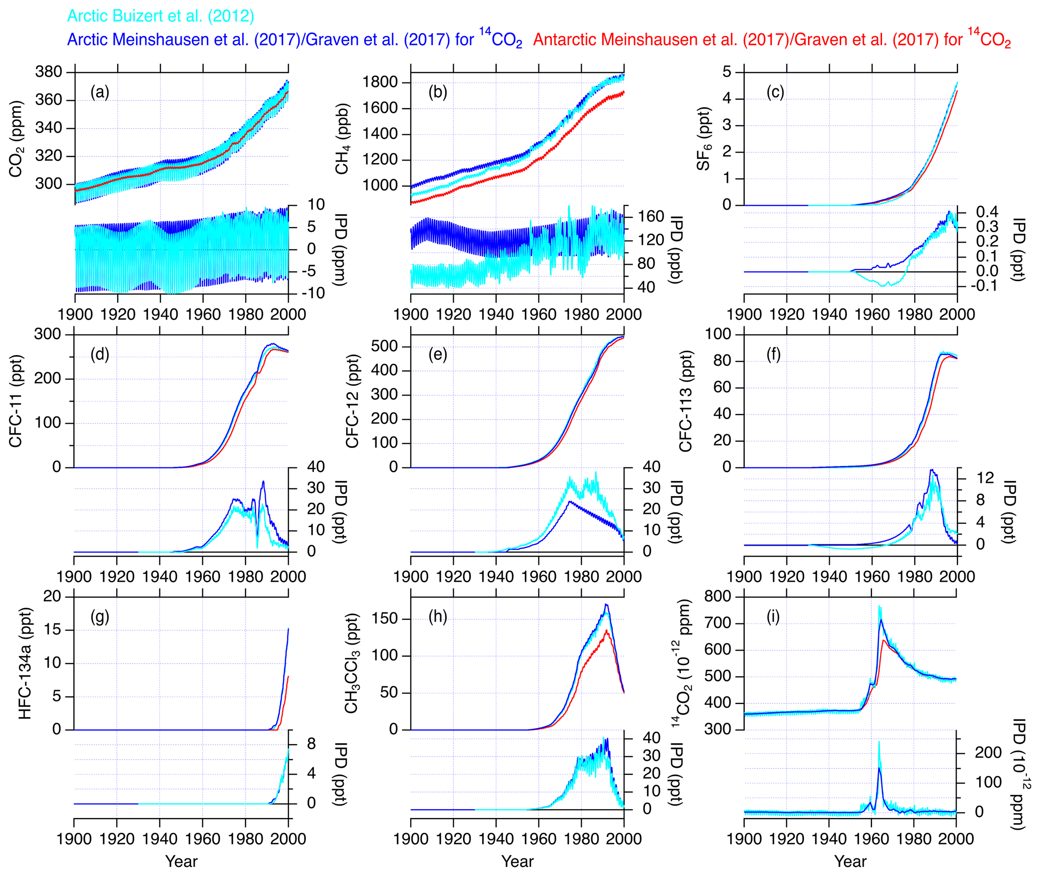
Figure 2Atmospheric scenarios of various trace gases used in this study. The Arctic histories prepared for the NEEM firn air modelling (Buizert et al., 2012) are in light blue. The Arctic and Antarctic histories for CMIP6 (Meinshausen et al., 2017) are in blue and red, respectively. For 14CO2, the CMIP6 historical data are from Graven et al. (2017). The interpolar differences (IPDs) calculated from the Arctic histories with respect to the Antarctic CMIP6 histories are also shown (right axes).
In contrast, the Arctic CH4 histories by the two studies differ considerably with maximum difference of ∼ 85 ppb around 1910 (Fig. 2b; see also Fig. 1). The two CH4 histories show similar trends after 1960, but before this, the data sets diverge further into the past. This disagreement is also clear in the interpolar difference (IPD), which is calculated relative to the CMIP6 histories for Antarctica (right axes). Note that the CMIP6 scenario for the Antarctic latitude was constructed based on the Law Dome ice core data (see the agreement in Fig. 1). While the BZ scenario shows a gradual increase in IPD, the CMIP6 scenario indicates almost constant values of IPD at ∼ 130 ppb over the 20th century. This difference stems from the different methodologies that were used to produce the respective scenarios. As described by Buizert et al. (2012), the BZ CH4 scenario was constructed by adding the presumed IPD to the Antarctic history (the Law Dome data), where the IPD was assumed to be proportionally correlated with the growth rate of CH4. This seems to be a reasonable assumption, given that the IPD and growth rate are both largely subject to changes in emissions from the Northern Hemisphere (Dlugokencky et al., 2003; Ghosh et al., 2015; Chandra et al., 2021). Meinshausen et al. (2017) compiled historical measurement records from the worldwide networks and Antarctic/Greenland ice core and firn samples and constructed latitudinally gridded data sets of various greenhouse gases. For the historical trend of CH4, they relied on the data set from the NEEM-S1 ice core by Rhodes et al. (2013) to produce the atmospheric histories for the Northern Hemisphere. They used the 5-yearly averaged values with outliers removed to represent lower bounds of the raw data points, as shown in Fig. 1. Note that the Rhodes et al. (2013) data set was not available when the BZ scenario was constructed. Thus, CH4 is unique because currently it has two diverging synthetic Arctic histories that are only loosely constrained by observational data.
This study assumes that the atmospheric scenarios for trace gases other than CH4 are known with sufficient accuracy. The scenarios of the individual trace gases have inherent uncertainties, but the comparisons of the two available scenarios (BZ and CMIP6) indicate that the data sources for other gases do not show inconsistent variations, as seen in CH4. It should be, however, noted that, except for CO2, many trace gases lack observational data for the early 20th century. Thus, both scenarios are, to a large extent, based on the same data sources.
3.3 Effective diffusivity
We follow the previous firn air studies in which the effective diffusivity in firn is optimised with an iterative method so as to minimise the difference between the simulated and observed depth profiles of CO2 (Sugawara et al., 2003; Ishijima et al., 2007). In these previous studies, an initial guess of the depth profile of effective diffusivity for CO2, Dinit(z), was calculated as follows:
where s(z) and D0 represent the open porosity at a depth z and the diffusion coefficient of CO2 at 253 K and 1013 hPa, respectively. D0 was set to 1.247 × 10⁻⁵ (m2 s−1) according to Trudinger et al. (1997). p is the mean atmospheric pressure (Pa). The bulk density (kg m−1) was determined by measuring the dimension and weight of cylindrically cut firn core samples (Kawamura et al., 2006). The effective diffusivity of CO2, thus obtained, was converted to those of other trace gases by multiplying by scaling factors from Buizert et al. (2012). Therefore, the depth profile pattern of the effective diffusivity is identical among all gases, but the magnitude is gas dependent due to the scaling factors. In this study, the effective diffusivity profile prepared for the NGRIP firn by Ishijima et al. (2007) is referred to as the initial diffusivity, and it was modified to improve the reproducibility of our newly measured trace gas profiles. For simulating trace gas profiles for the NEEM firn, we began with the effective diffusivity profiles available from Buizert et al. (2012). Those effective diffusivity profiles, which were originally optimised for individual firn air transport models that participated in that study, were modified and used for simulating the various trace gas profiles reported for the NEEM firn. The various diffusivity profiles were constructed by modifying the original profiles at a certain range of depths in a stepwise empirical manner; the depth range of the diffusivity profile key to improve reproducibility of trace gas depth profiles was first diagnosed and then the diffusivity was perturbed up and down in the depth range to the degree in which the corresponding simulated profiles do not deviate substantially. Although this simple method does not guarantee identification of a best-match profile, we are confident that an acceptable range of the diffusivity profile is satisfactorily constrained.
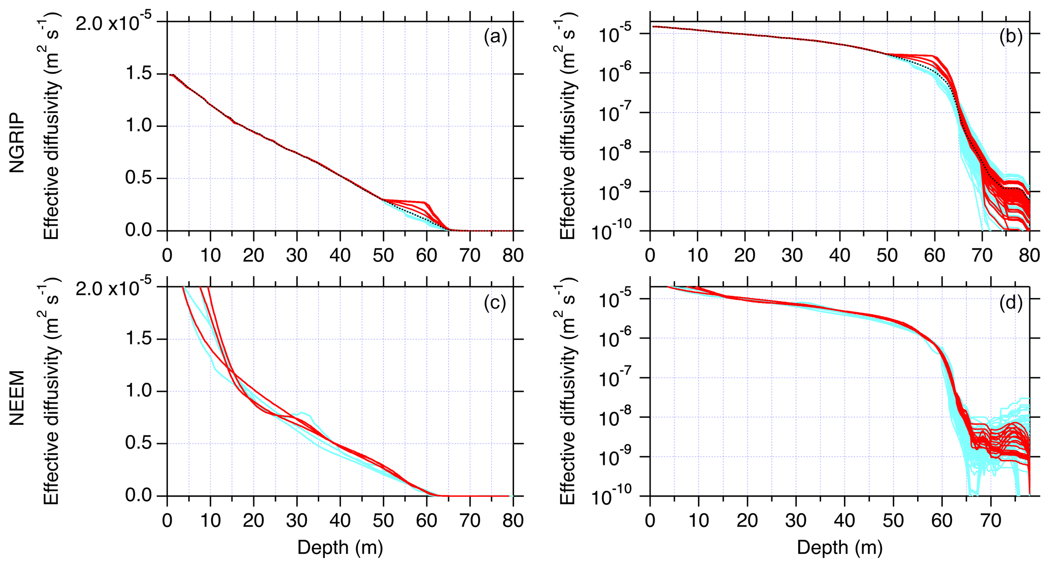
Figure 3The 100 sets of effective diffusivity profiles of CO2 in the NGRIP (a, b, where panel a is on a linear scale and panel b is on a log scale) and NEEM firn (c, d). The initial diffusivity profile (Ishijima et al., 2007) is shown by a black dotted line (NGRIP only) and modified diffusivity profiles are in colours. The diffusivity profiles whose corresponding mole fraction profiles have root mean square deviation (RMSD) values of < 1.0 are coloured red and the others light blue.
We eventually prepared 100 different sets of diffusivity profiles so as to cover a considerable range of diffusivity. Each set of the diffusivity profiles was evaluated based on the root mean square deviation (RMSD) between the model and data, according to Buizert et al. (2012). All sets of effective diffusivity profiles for the NGRIP and NEEM firn sites are shown in Fig. 3 (top and bottom panels, respectively). The different colours of the diffusivity profiles will be explained later. Those diffusivity profiles were evaluated against the observed trace gas profiles, which were regarded as constraints. Note that CH4 was not used in the evaluation, and the atmospheric scenarios of other trace gases are assumed to be known with sufficient accuracy to infer a range of acceptable diffusivity profiles that reproduce the depth profiles of the firn air composition.
3.4 Performance of the firn air transport model
To validate our firn air transport model, we began by simulating depth profiles of various trace gases in the NEEM firn. Our model did not participate in the model intercomparison study using the NEEM data (Buizert et al., 2012). In this simulation, we employed the BZ scenarios as per their model intercomparison. The simulated depth profiles of the nine trace gases are presented in Fig. 4 and compared with those by other models presented in Buizert et al. (2012). The results confirm that the performance of our model is comparable to those by other groups. As a measure of the model performance, Buizert et al. (2012) compared RMSD, which ranged from 0.73 to 0.92 for the six participating models. Following the same approach, our model yields the RMSD value of 0.83 for the NEEM EU borehole. This RMSD value was achieved with an effective diffusivity profile that was prepared by modifying the profile originally optimised for the CIC (Centre for Ice and Climate) model at a certain range of depths. Note that the RMSD value here was calculated to include CH4, as per Buizert et al. (2012), but, as described in Sect. 3.5, CH4 is excluded in calculation of RMSD in the following sections.
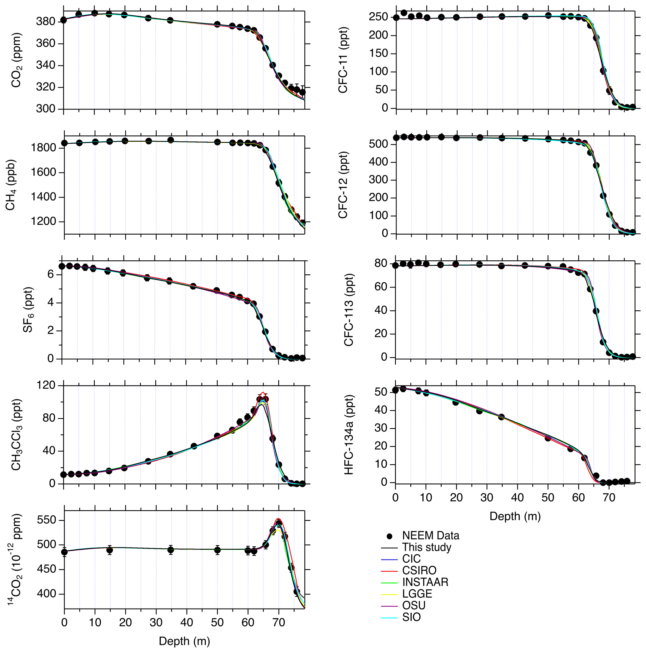
Figure 4Modelled depth profiles of various compounds in the NEEM firn. Closed circles in black are the observed data with uncertainty estimated by Buizert et al. (2012). Our model results are shown with black solid lines, and the results from other models are in colours. Different models are labelled by institution, according to Buizert et al. (2012), as follows: CIC (Centre for Ice and Climate), CSIRO (Commonwealth Scientific and Industrial Research Organisation), INSTAAR (Institute of Arctic and Alpine Research), LGGE (Laboratoire de Glaciologie et Géophysique de l'Environnement), OSU (Oregon State University), and SIO (Scripps Institution of Oceanography).
3.5 Reconstruction of CH4 history
Our modelling procedure for reconstructing the atmospheric histories of CH4 was as follows:
-
To represent atmospheric trends of different trace gases in the Arctic region, we began by employing the two sets of atmospheric scenarios (Sect. 3.2). The firn transport model calculates depth profiles of the various trace gases at the NGRIP and NEEM firn sites using the large set of modified (N=100) effective diffusivities described in Sect. 3.3. The simulation case with each diffusivity profile was evaluated based on RMSD. As we aim to estimate the historical atmospheric trend of CH4, the RMSD-based evaluations were made using all of the available trace gas data, excluding CH4. In the RMSD calculation, we used the measurement uncertainties of 0.2 ppm for CO2, 0.2 ppt for SF6, 1.1 ppt for CFC-11, 3.3 ppt for CFC-12, 0.6 ppt for CFC-113, and 3.2 ppt for CH3CCl3 for the NGRIP firn. For the NEEM firn, we employed the uncertainties provided by Buizert et al. (2012). It should be noted that the present study does not follow the uncertainty estimation as done by Buizert et al. (2012). They indicated that uncertainties in the atmospheric scenarios and measurement uncertainties are the two largest contributors to the total uncertainties for individual data points for the NEEM firn. We consider that the uncertainties in the atmospheric scenarios are appreciably examined through comparisons of series of simulations using the two independent scenarios.
-
We ran the model with 100 different sets of diffusivity profiles to calculate the depth profile of CH4. Note that, based on the earlier step, we know the diffusivity profiles that generate reasonable firn air profiles for the trace gases other than CH4. Every diffusivity profile was used in combination with the firn air CH4 data for reconstructing an atmospheric CH4 history. We employed an iterative dating approach (Trudinger et al., 2002), where the initial atmospheric scenario (the BZ scenario) was modified to improve model reproducibility of the CH4 depth profile (see below). The corrected atmospheric CH4 scenarios were then compared to the original scenarios (BZ and CMIP6) for further discussion.
The iterative dating for CH4 was performed as follows:
- i.
The depth profile of CH4 was calculated with the initial atmospheric CH4 scenario.
- ii.
The modelled CH4 mole fraction, calculated in step (i), was compared to the input atmospheric CH4 scenario, and an effective age at each sampling depth was determined as the time when the modelled CH4 agreed with a value in the atmospheric CH4 scenario. It is noted that the smoothing spline curve applied to the BZ CH4 scenario was used for the calculation of the effective age, as the input scenario with seasonal variation (Fig. 2) would not allow the effective age to be uniquely determined.
- iii.
A new atmospheric CH4 scenario was constructed by assigning the observed CH4 mole fraction, at each sample depth, to the effective age determined in step (ii). The observed CH4 versus the effective age data set was interpolated by a smoothing spline function, and it is considered as a revised atmospheric CH4 scenario.
- iv.
The depth profile of CH4 was again calculated with the revised atmospheric CH4 scenario constructed in step (iii).
- v.
The above steps (ii–iv) were repeated until the model–data difference converged within an acceptable range (typically after a few iterations; Trudinger et al., 2002; Ishijima et al., 2007). In this study, we made five iterations for each modified diffusivity case as we confirmed sufficient convergence of the result.
4.1 Initial simulations: NGRIP
Figure 5 presents the simulation results with the initial diffusivity in comparison to the observed profiles for the six trace gases, excluding CH4 (CO2, SF6, CFC-11, CFC-12, CFC-113, and CH3CCl3) for the NGRIP firn. It is again noted that the initial diffusivity profile was tuned only for the depth profile of CO2 (Ishijima et al., 2007). As seen in this figure, measured profiles of these trace gases (except CH3CCl3) show gradual decreases with depth in the DZ and sharp decreases in the LIZ. In contrast, CH3CCl3 increases with depth in the DZ and sharply decreases in the LIZ. The difference in the depth profile pattern among species is due to their different historical atmospheric trends. It is known that, since the mid-20th century, the atmospheric mole fractions of the five trace gases (CO2, SF6, CFC-11, CFC-12, and CFC-113) have increased either monotonically or shown peak/slowed increase in the early 1990s (Sturrock et al., 2002; Martinerie et al., 2009). In contrast, CH3CCl3 increased until the early 1990s and has rapidly decreased since then (Sturrock et al., 2002; Rigby et al., 2017), which is also observed in Fig. 2. Our simulation reproduces the observed depth profiles of these six trace gases in the NGRIP firn fairly accurately by using the BZ scenarios.

Figure 5Depth profiles of CO2, SF6, CFC-11, CFC-12, CFC-113, and CH3CCl3 in the NGRIP firn. The measurement and model results are shown by red circles and black solid lines, respectively (left axis). The measurement uncertainties are shown as vertical error bars, though in many cases they are smaller than the circle sizes. Black solid lines show the modelled profiles with the initial diffusivity and the BZ scenarios. The black dashed lines indicate the profiles calculated with the atmospheric scenarios for Antarctica (red lines in Fig. 2). The model–data differences are also shown (right axis). The vertical solid line in each panel indicates the upper depth of LIZ.
It is interesting to note that the depth profiles of CH3CCl3 at NGRIP and NEEM are remarkably different. Whereas the NEEM data show a relatively sharp CH3CCl3 peak in the LIZ (∼ 65 m; Fig. 4), NGRIP does not show such a narrow peak. This is due to the timing of firn air sampling i.e. 2001 for NGRIP and 2008 for NEEM. When the NGRIP firn air was sampled, the signal of the maximum atmospheric CH3CCl3 in the early 1990s had only reached near the top of the LIZ at the site, thereby formulating the relatively gentle changes at the shallower depths. On the other hand, 7 years later, at the NEEM site, such a signal was found deeper in the LIZ, where the age of air changes rapidly with depth in both deeper and shallower sides. We emphasise that, despite the differences in the depth profiles of CH3CCl3 at the two sites, our simulations reproduce the profiles measured at both sites well when using the same atmospheric CH3CCl3 scenario.
4.2 Sensitivity to diffusivity profile: NGRIP
Figure 5 shows that the model–data difference increases in the LIZ for all the trace gases. In particular, the model–data difference is pronounced as a dip around 70 m for all trace gases, implying that the mismatches may originate in a common factor in the modelling, e.g. a depth profile of diffusivity. To examine the impact of diffusivity modification on the simulated depth profiles and their agreements with the data, we examined the 100 sets of modified diffusivity profiles (Fig. 3). It was found that, to reduce the model–data difference in the LIZ (Fig. 5), the diffusivity needs to be increased in the shallower layers compared with the top LIZ, i.e. 50–65 m. The diffusivity was also modified in the deeper layers (> 65 m), and simulations were made accordingly. The simulated profiles for depths deeper than 50 m using the 100 diffusivity profiles are presented for the six trace gases (Fig. 6). In this figure, the modelling results with the modified diffusivity profiles are shown in colours on the left axis, and the model–data differences of the respective cases are plotted on the right axis. It is clear that the model–data differences could be significantly reduced with some diffusivity cases. The RMSD values are as little as 0.51 for a particular case. In Fig. 6 and associated figures, the model results with RMSD of < 1.0 are coloured red and other cases are coloured light blue.
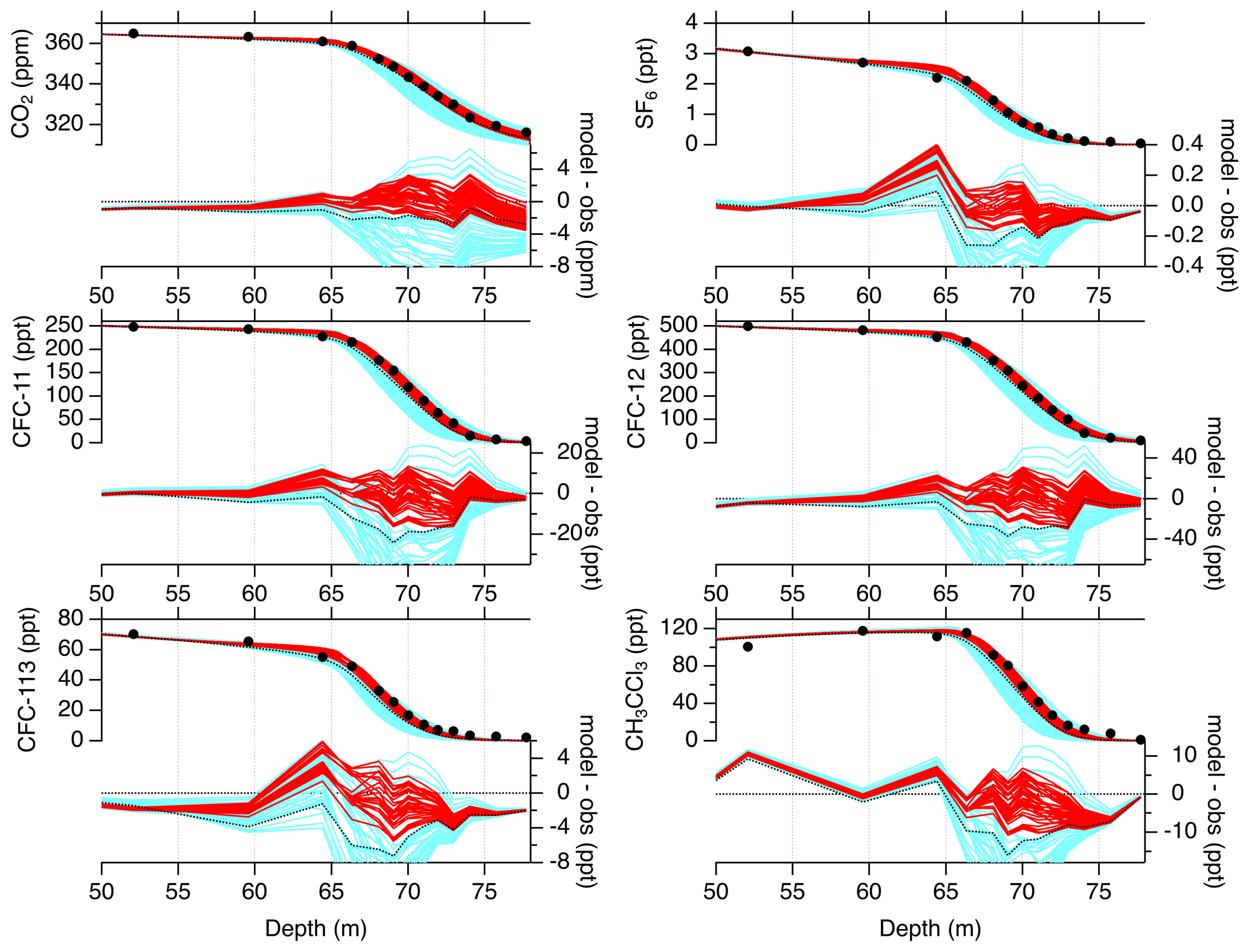
Figure 6Depth profiles of the six trace gases below 50 m depth in the NGRIP firn. Black circles indicate the measurements, and solid lines in colours are the model results with different diffusivity profiles and the BZ scenarios (left axis). Black dotted lines are modelled results with the initial diffusivity. Also shown are the model–data differences (right axis). See the text for the differences in the line colours.
4.3 Sensitivity to atmospheric scenario: NGRIP
In Fig. 7, modelled depth profiles with different sets of the atmospheric scenarios (BZ and CMIP6) are compared for trace gases other than CH4. For simplicity, only the results with RMSD of < 1.0 are presented. This figure shows that the differences in the atmospheric histories (Fig. 2) produces relatively small differences in the depth profiles in the firn. There are small offsets due to the differences of the histories in some gases; the difference in the SF6 history before 1980 (< 0.2 ppt) corresponds to the small (< 0.1 ppt) offsets below 65 m, significant differences in the histories of CFC-11 (< 10 ppt) and CFC-12 (< 20 ppt) for 1960–1990 resulted in the overall offsets (roughly < 5 and < 10 ppt, respectively) below 50 m, and the difference in the CH3CCl3 history (< 10 ppt) in the early 1990s produced the offsets (∼ 3 ppt) above 66 m. The smaller offsets in the calculated depth profiles than in the input atmospheric scenarios are due to the smoothing effect of diffusion in the firn layers. We calculated the difference between the modelled profiles with the two scenarios for individual diffusivity cases and found that those differences in the LIZ are within the measurement precisions for SF6, CFC-113, and CH3CCl3. They are a bit larger for CO2, CFC-11, and CFC-12, which are up to 5 times the respective measurement precisions.

Figure 7Same as Fig. 6 but for a comparison of the modelled profiles in the NGRIP firn with different atmospheric scenarios of BZ and CMIP6, which are shown in light blue and green, respectively. Only the simulation results with RMSD values of < 1.0 are shown.
4.4 Simulations of CH4: NGRIP
Modelled depth profiles of CH4 are shown in Fig. 8. These calculations were made with the 100 diffusivity profiles and the atmospheric CH4 scenarios of BZ (left) and CMIP6 (right). It is interesting to note that the characteristics of the model–data difference for CH4 are different from those for the other six trace gases (Fig. 6). For the other trace gases, the initial simulation showed increased model–data differences around 70 m, and they were reduced with some modified diffusivity profiles. For CH4, the model run with the initial diffusivity profile and the BZ scenario reproduces the observed CH4 profile quite well down to ∼ 73 m but significantly overestimates by > 20 ppb for the lowest three depths (the black dotted line in the left panel). Using the modified diffusivity profiles that allowed better agreements for the other six trace gases (red lines), we find larger model–data CH4 differences than in the initial simulation. These features are also seen for the simulation results with the CMIP6 scenario (right panel), but the overestimate in the LIZ is more pronounced because the CH4 mole fractions for the early- to mid-20th century are higher in the CMIP6 than in the BZ scenario. In comparison to other gases (Sect. 4.3), the largest impact of the scenario difference occurs in CH4. In the LIZ, the difference between depth profiles with the two scenarios reaches to 5–10 times the measurement precision, namely > 30 ppb in some diffusivity cases.
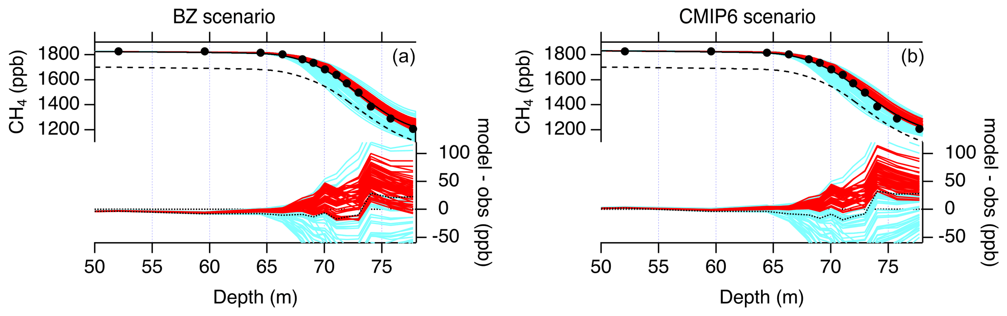
Figure 8Same as Fig. 6 but for CH4 in the NGRIP firn. Simulation results with the atmospheric scenarios of BZ and CMIP6 are shown in panels (a) and (b), respectively. The black dashed lines indicate the profiles calculated with the atmospheric scenarios for Antarctica (red line in Fig. 2).
4.5 Sensitivity to IPD: NGRIP
Reflecting geographical source/sink allocation and atmospheric lifetime, different trace gases show a different magnitude of IPD, as shown in Fig. 2. It would be possible that, for some gases, the northern to southern difference in mole fraction has little influence on depth profile in firn due to the relatively small interhemispheric gradient. To examine magnitude of the sensitivity of the depth profiles to the IPD for individual trace gases, we calculated the depth profiles that would be expected if the Antarctic atmospheric scenarios (red lines in Fig. 2) are given to force the firn model for the NGRIP firn. The results are shown by dashed lines in Fig. 5. This sensitivity experiment shows that IPD causes significant biases larger than the measurement precisions of the respective trace gases. We calculated the difference between the simulations for the BZ scenario (solid line) and the Antarctic scenario (dashed line) and found that sensitivities to the IPD for these six trace gases are no more than 20 times the respective measurement uncertainties. Such relative sensitivities of these suite of gases to the IPDs are much smaller than that of CH4, which reaches 40 times the measurement uncertainty. As seen in Fig. 8, the calculated CH4 profile with the Antarctic scenario for the NGRIP firn is aligned ∼ 120 ppb below the original simulation, showing the pronounced impact on CH4.
4.6 Sensitivity to atmospheric scenario: NEEM
In addition to the above simulations for the NGRIP firn, we examined the impact of the difference of the atmospheric scenarios on the depth profiles for the NEEM firn. In Fig. 9, comparisons between simulations with the different scenarios for the nine trace gases, including CH4, are presented. We found some common characteristics at the NGRIP and NEEM firn sites. While the difference between the simulations with the two scenarios are relatively small for most trace gases, the large difference between the CH4 scenarios (i.e. higher CH4 mole fraction in the CMIP6 scenario; see Fig. 2) results in an overestimation of CH4 mole fraction in the LIZ (> 63 m) in the modelled profiles with the CMIP6 scenario. In the LIZ, the difference in the depth profiles with the two scenarios exceeds 30 ppb, which is comparable to the magnitude observed in the NGRIP firn (Fig. 8).

Figure 9Same as Fig. 7 but for the NEEM firn. Only the simulation results with RMSD values of < 1.0 are shown.
4.7 Reconstruction by iterative dating
As shown in the earlier sections, CH4 shows uniquely high uncertainty in the firn modelling compared to other trace gases. First, simulated depth profiles of CH4 do not show improved reproducibility with effective diffusivity profiles that satisfy depth profiles of other gases (Sect. 4.2 and 4.4). Second, while other gases show limited sensitivities to the different atmospheric scenarios, inconsistency between the currently available two scenarios have particularly large impact on the simulated depth profile of CH4 (Sect. 4.3 and 4.4). Third, sensitivity to IPD in the atmospheric scenarios is most pronounced for CH4 compared to other trace gases (Sect. 4.5). These characteristics are common for both NGRIP and NEEM sites (Sect. 4.6).
Taking all these unique characteristics of CH4 into account, we explore the possibility of reconstructing the Arctic CH4 mole fractions by the iterative dating method. This approach has a fixed diffusivity profile (assumed to be correct) and aims to find an acceptable atmospheric history to reproduce the firn air depth profile. It is considered that the modified diffusivity profiles with the low RMSD values are adequately evaluated by the trace gases, except CH4, and that the model–data mismatch in the CH4 modelling is therefore attributable to uncertainty in the atmospheric CH4 scenario. The historical atmospheric CH4 variations obtained by the iterative dating method are presented in Fig. 10 for the 100 modelling cases of the modified diffusivity. The different simulation cases are coloured in the same manner as in the earlier figures according to the RMSD (Figs. 3, 6, and 8). Note that the reconstruction cases coloured in light blue are considered to be less likely due to poorer reproduction of the depth profiles (Figs. 6 and 8). The NGRIP reconstruction results (red; Fig. 10a) are in good agreement with the BZ scenario after around 1980. For the earlier period, however, the upper bounds of the reconstructions (line connecting far-left red circles) match with the BZ scenario, and the overall range of acceptable histories is below the BZ scenario (circles and shades in red). On the other hand, the NEEM reconstruction results show that the range of acceptable histories are distributed closely around the original BZ scenario or below it after around 1960, whereas the lower bounds of the reconstruction (line connecting far-right red circles) align with the BZ scenario before that (Fig. 10b).
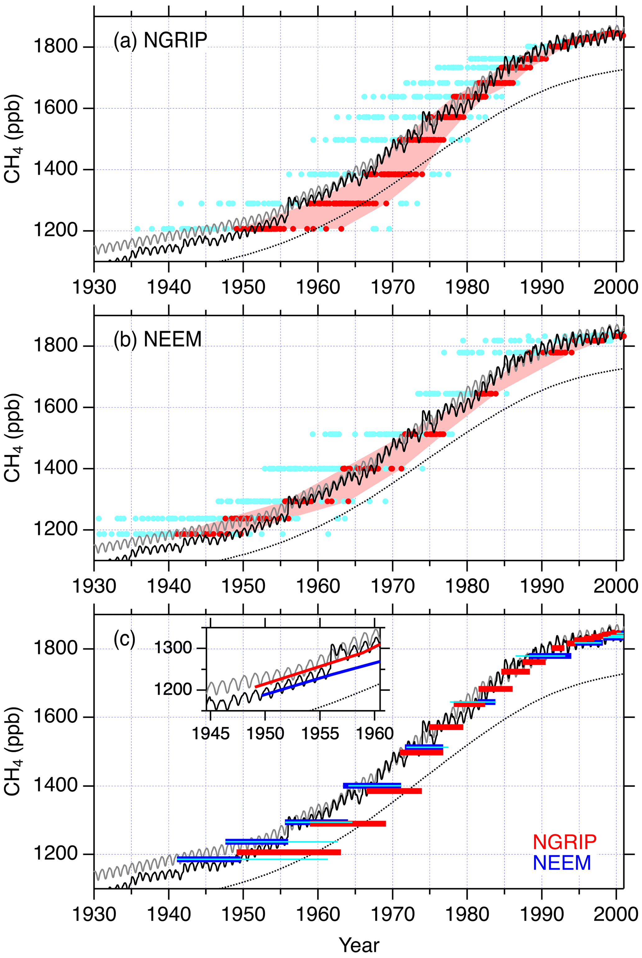
Figure 10Results of reconstructions by the iterative dating method for the model cases with the 100 different diffusivity profiles (circles coloured in the same manner as in Figs. 3, 6, and 8) from the (a) NGRIP and (b) NEEM firn air and (c) the ranges of reconstructions from both firn sites. The red shades indicate the range of CH4 mole fraction trends reconstructed using the diffusivity profiles that better reproduce the trace gases, except for CH4. Black and grey solid lines are the atmospheric CH4 scenarios of BZ and CMIP6, respectively, and the black dotted line is the smoothed Antarctic CH4 mole fraction (spline curve) from the Antarctic data shown in Fig. 1. The thick horizontal bars in red and blue in panel (c) correspond to red shades in panels (a) and (b). The light blue thin bars in panel (c) indicate the range of the reconstructions for cases in which 14CO2 data are excluded for evaluations of the diffusivity profiles. The inset in panel (c) shows the magnified view of the NGRIP upper bounds (red) and the NEEM lower bounds (blue) in comparison to the two scenarios.
It should be stressed that the reconstructions for the time period before 1980 rely on CH4 data from the lowest four or five depths of the NGRIP and NEEM firn air. The differences between the initial and corrected atmospheric CH4 scenario from the three deepest data for the NGRIP firn are up to ∼ 100 ppb. As seen in Fig. 10, such a reduction in the Arctic atmospheric CH4 scenario over the period would result in alignment with the atmospheric CH4 trend in Antarctica inferred from the Law Dome and other data sets (black dotted line). It is again noted that all the reconstruction cases coloured in red used diffusivity profiles that yield relatively good model reproducibility with RMSD values of < 1.0. It is therefore seen that iterative-dating-based reconstruction from the NGRIP firn data suggests lower CH4 mole fraction than the BZ or CMIP6 scenarios from the 1950s to 1970s in any case, albeit with large uncertainty. It is, however, noted that, as shown in Fig. 10c, this result is not fully compatible with that from the NEEM firn. In particular, the discrepancies between the reconstructions from both firn data diverge with time before 1970. When compared to these reconstructions, the BZ scenario (black line) tracks the overlapping ranges of both reconstructions, while the CMIP6 scenario passes above them before around 1955.
5.1 CH4 history
In Sect. 4, we have shown that, with the two atmospheric scenarios (BZ and CMIP6), depth profiles of CO2, SF6, CFC-11, CFC-12, CFC-113, and CH3CCl3 in the NGRIP and NEEM firn are reproduced with sufficient accuracy by using a range of modified diffusivity profiles (Figs. 6, 7, and 9). This suggests that the atmospheric scenarios of these trace gases used in the modelling are consistent with the depth profiles observed at both firn sites in Greenland (NEEM and NGRIP). In contrast, the observed CH4 profile in the NGRIP firn was not accurately reconciled using the two atmospheric scenarios and the diffusivity profiles that allow adequate reproducibility for the trace gases (except CH4). This suggests either that the Arctic atmospheric scenarios of CH4 are uncertain or that the diffusivity profile of the NGRIP firn is underconstrained. We explored the correction of the atmospheric scenario of CH4 by using the iterative dating approach. This method improves agreement to the observed CH4 depth profile, with an implicit assumption that the diffusivity profile in each case is correct. Although uncertainty due to the underconstrained diffusivity profile in the LIZ is large, this attempt for the NGRIP firn suggested that the CH4 mole fractions over the period 1950–1980 could be ∼ 100 ppb lower than the original BZ scenario (Fig. 10). In contrast, the iterative dating reconstruction for the NEEM firn agrees with the BZ scenario. Although the spread of the reconstructions is large, particularly for the NGRIP firn, it was found that the BZ scenario passes within the ranges of the reconstructions from both firn data but that the CMIP6 scenario is notably higher than the reconstructions for the period before 1960.
Whereas uncertainties in the reconstructions from the individual firn sites are large, Fig. 10c could suggest a relatively narrow range of the CH4 history that satisfies both NGRIP and NEEM reconstructions. Although the overlapping range of the two reconstruction is ∼ 90 ppb in the 1970s, it is as small as ∼ 30 ppb in the 1950s. This suggests that the combined NGRIP and NEEM firn data could provide a stronger constraint to the range of the CH4 mole fraction, e.g. 1185–1215 and 1225–1260 ppb in 1950 and 1955, respectively (Fig. 10c inset). It is again noted that only the BZ scenario fall within these ranges for the period, suggesting that it is likely closer to the true atmospheric CH4 history than the CMIP6 scenario for the mid-20th century.
The IPD of the atmospheric CH4 mole fraction is important for a better understanding of the evolution of the global CH4 budget. Given that the Antarctic ice core and firn measurements have provided relatively reliable CH4 records over the 20th century, improved reconstructions from Greenland ice cores and firn air should better constrain the changes in the IPD. To sufficiently constrain the historical global CH4 budget, the reconstruction for Greenland needs to be accurate within ∼ 10 ppb, corresponding to ∼ 30 Tg CH4 yr−1 global emission. Based on the current best firn CH4 data from NGRIP and NEEM, we demonstrated that consistent reconstruction of the Arctic CH4 mole fraction is achievable back to the 1950s, but the uncertainty of the reconstruction is still large (> 30 ppb) for the 1950s to 1970s.
5.2 Uncertainty of effective age
It is important to note that the reconstructions for the period before 1980 from the NGRIP firn were heavily influenced by the five deepest data in the LIZ (> 72 m). Figure 11a shows distributions of the effective age of CH4 at depths below 55 m in the NGRIP firn, which is coloured the same as in the earlier figures. In addition, the spread of the effective age (σage) at each sampling depth is shown on the right axis. This figure shows that firn air samples collected at the five lowest sampling depths at NGRIP have effective ages corresponding to the period from ∼ 1950 to the late 1970s. At those depths, even the acceptable diffusivities yield the spread of the effective age of > 5 years (black vertical bars). This shows that the reconstruction of the CH4 mole fraction for the period is subject to much uncertainty in effective age. For the NEEM firn, the reconstructions before 1980 also rely on the five deepest data in the LIZ (Fig. 11b). The σage values at those depths in the NEEM firn range from 5 to 8 years (thick vertical bars), comparable to those in the NGRIP firn. The Antarctic atmospheric CH4 record (see Figs. 1 and 10) indicates that the atmospheric increase rate of CH4 was 10–15 ppb yr−1 over the period. The 5-year uncertainty in the age estimate for the NGRIP firn air samples could therefore be translated to an uncertainty of > 50 ppb in the Arctic atmospheric CH4 level. This is comparable to the IPD of CH4 mole fraction during the 1950s to 1970s, which was assumed when Buizert et al. (2012) prepared the BZ CH4 scenario.

Figure 11Depth profiles of effective age of CH4 calculated after the iterative dating calculations for depths below 55 m at the (a) NGRIP and (b) NEEM firn sites (left axis). The solid lines represent cases for different diffusivity profiles and are coloured in the same manner as in the earlier figures. Vertical bars in black indicate the spread of the effective age (σage; maximum minus minimum) at the individual sampling depths among the modelling cases in red (right axis). For the NEEM firn, the thin vertical bars correspond to the spread for simulation cases in which 14CO2 data are excluded for evaluations of the diffusivity profiles.
It is also interesting to note that σage at the four deepest depths in the NEEM firn is almost constant, whereas it increases with depth in the NGRIP firn and exceeds 10 years at the two deepest depths. This indicates that effective age in the oldest firn air layers can be estimated with better accuracy in the NEEM firn than in the NGRIP firn, thereby providing the reconstructions with smaller uncertainties. As σage was calculated from the simulation cases with acceptable ranges of diffusivity, its magnitude reflects how tightly the diffusivity profile is constrained at each firn site. In other words, our simulations infer that the diffusivity profile in the NEEM firn can be better constrained than the NGRIP firn.
5.3 Constraint to diffusivity profile
In order to see the degree of constraint to the effective diffusivity from different trace gases, we calculated RMSD values for different combinations of the trace gases for the NEEM firn. The choice of the NEEM firn is due to the availability of a larger number of gas species. It was found that the 14CO2 data provide strong constraints for narrowing the acceptable range of diffusivity profiles in the LIZ, as its history has a unique peak in the early 1960s due to nuclear weapons testing (Fig. 2). The evaluated RMSD, with the 14CO2 data excluded and the historical CH4 reconstruction from the simulation cases with RMSD < 1.0, is presented in Fig. 10c (thin horizontal bars in light blue). The corresponding spread of the effective age is also shown in Fig. 11b (thin vertical bars in black). These results show that, for the NEEM reconstruction, the uncertainty of the effective age would be doubled at the two deepest depths if it were not for the 14CO2 data. It is also interesting that the range of the CH4 reconstruction without 14CO2 would deviate in the younger ages and would suggest a historical trend lower than the BZ scenario (Fig. 10c). In turn, the CH4 trend reconstructed from the NGRIP firn might be different if the 14CO2 measurement was available. The above contribution of the 14CO2 data for the NEEM firn implies that the NGRIP reconstruction could have been closer to the NEEM reconstruction. It is also noted that constraints from halocarbon species to the diffusivity profile are relatively weak, as their mole fractions in the LIZ decreased to close to zero.
5.4 Outlook
Previous studies have used CH4 as one of tracers that constrain diffusivity profiles in firn (Witrant et al., 2012; Trudinger et al., 2013). These studies have shown that CH4 effectively contributed to constraining diffusivity for deep layers, i.e. LIZ in the NEEM firn. However, the use of CH4 as an effective constraint is valid only when its atmospheric scenario given as input to the models was assumed to be correct. Figs. 6 and 8 show a larger spread in the model–data differences of CH4 among the different diffusivity cases spread widely in the deepest layers of the LIZ of the NGRIP firn, in comparison to the other six gases. This fact highlights that subtle changes of the diffusivity profile in the LIZ have a large impact on simulating CH4, and it indeed indicates that the species could serve as an effective diffusivity constraint if its atmospheric scenario was correctly given with low uncertainty. This study indicated that the two currently available Greenland firn data sets (NGRIP and NEEM) are more consistent with the BZ CH4 scenario (Buizert et al., 2012) than the CMIP6 scenario (Meinshausen et al., 2017). Furthermore, it should be again pointed out that the CMIP6 scenario suggests an almost constant IPD of ∼ 130 ppb over the 20th century (Fig. 2). Such constant IPD is unlikely because CH4 emissions are considered to have increased in the Northern Hemisphere for that period, which requires IPD to increase with time as discussed in the previous studies (Dlugokencky et al., 2003; Ghosh et al., 2015; Chandra et al., 2021). Accordingly, the BZ scenario appears to be a useful choice in firn modelling at Greenland sites, but it should be kept in mind that the use of CH4 as a tuning tracer could lead to overfitting of the diffusivity profile.
A possibility to improve the reproducibility of the depth profile of CH4 in the NGRIP firn could come from an additional constraint to the diffusivity profile, along with those currently made by the six trace gases (CO2, SF6, CFC-11, CFC-12, CFC-113, and CH3CCl3). In particular, it was indicated that 14CO2, if available, would have strongly constrained the diffusivity profile and reduced the uncertainty of the historical CH4 trend reconstructed from the NGRIP firn. This study showed that the currently available firn data from Greenland (NGRIP and NEEM) are in better agreement with the historical CH4 scenario prepared for the NEEM firn modelling (Buizert et al., 2012) than that for the CMIP6 experiments (Meinshausen et al., 2017). Since the latter scenario relies on the NEEM-S1 ice core data (Rhodes et al., 2013), this study highlighted inconsistency between the ice core and two sets of firn data in Greenland. Given that reconstruction of the CH4 history from the deepest firn layers is challenging (in terms of the diffusivity versus history problem, as shown in this study), future sampling and measurements of ice cores at a high-accumulation site in Greenland (where the age of the air occluded can be determined accurately) may be the only way to reconstruct the atmospheric CH4 trend over the 20th century.
The composition data of the NGRIP firn air samples are available on the Arctic Data archive System (ADS) of National Institute of Polar Research (https://doi.org/10.17592/001.2021060901; Kawamura et al., 2021b). The NEEM firn air data are available in the supplementary file of Buizert et al. (2012). The CMIP6 historical scenarios of the various trace gases used in this study are available via https://esgf-node.llnl.gov/search/input4mips/ (last access: 25 October 2021), as described in Meinshausen et al. (2017). Those of 14CO2 are available in the supplementary file of Graven et al. (2017). Our modelling data are available upon request (umezawa.taku@nies.go.jp).
TU, SS, KK, and IO discussed on design of the study. KK, SA, and TN conducted firn air sampling at the NGRIP site. SS, KK, TU, and TS analysed the firn air samples for trace gases. SJA set up the measurement system for the halocarbons. TU and SS made firn air model simulations. TU analysed the measurement/modelling data and prepared the paper with contributions from all co-authors.
The contact author has declared that neither they nor their co-authors have any competing interests.
Publisher’s note: Copernicus Publications remains neutral with regard to jurisdictional claims in published maps and institutional affiliations.
We thank Morimasa Takata, at the Nagaoka University of Technology, for assisting with the sample collection, and Jakob Schwander, at the University of Bern, for the collaboration at NGRIP. The NGRIP project was directed and organised by the Department of Geophysics at the Niels Bohr Institute for Astronomy, Physics and Geophysics, University of Copenhagen. It is supported by funding agencies in Denmark (SNF), Belgium (FNRS-CFB), France (IPEV and INSU/CNRS), Germany (AWI), Iceland (RannIs), Japan (MEXT), Sweden (SPRS), Switzerland (SNF), and the USA (NSF; Office of Polar Programs). We are grateful to the efforts of NOAA/ESRL/GML and the NEEM firn campaign, for the measurement and modelling data, both of which are made freely available. We thank the two anonymous referees, for the helpful comments that improved the paper.
This research has been supported by the Japan Society for the Promotion of Science KAKENHI Grants-in-Aid for Young Scientists B (grant no. 17K18342 for Taku Umezawa), Grants-in-Aid for Scientific Research on Innovative Areas (grant no. 17H06320 for Kenji Kawamura), Grant-in-Aid for Scientific Research B (grant no. 20H04327 for Ikumi Oyabu), and the MEXT GRENE Arctic Climate Change Research Project (for Shuji Aoki).
This paper was edited by Eliza Harris and reviewed by two anonymous referees.
Aoki, S., Nakazawa, T., Murayama, S., and Kawaguchi, S.: Measurements of atmospheric methane at the Japanese Antarctic Station, Syowa, Tellus B, 44, 273–281, https://doi.org/10.1034/j.1600-0889.1992.t01-3-00005.x, 1992.
Blunier, T., Chappellaz, J. A., Schwander, J., Barnola, J.-M., Desperts, T., Stauffer, B., and Raynaud D.: Atmospheric methane, record from a Greenland Ice Core over the last 1000 year, Geophys. Res. Lett., 20, 2219–2222, https://doi.org/10.1029/93GL02414, 1993.
Buizert, C., Martinerie, P., Petrenko, V. V., Severinghaus, J. P., Trudinger, C. M., Witrant, E., Rosen, J. L., Orsi, A. J., Rubino, M., Etheridge, D. M., Steele, L. P., Hogan, C., Laube, J. C., Sturges, W. T., Levchenko, V. A., Smith, A. M., Levin, I., Conway, T. J., Dlugokencky, E. J., Lang, P. M., Kawamura, K., Jenk, T. M., White, J. W. C., Sowers, T., Schwander, J., and Blunier, T.: Gas transport in firn: multiple-tracer characterisation and model intercomparison for NEEM, Northern Greenland, Atmos. Chem. Phys., 12, 4259–4277, https://doi.org/10.5194/acp-12-4259-2012, 2012.
Chandra, N., Patra, P. K., Bisht, J. S. H., Ito, A., Umezawa, T., Saigusa, N., Morimoto, S., Aoki, S., Janssens-Maenhout, G., Fujita, R., Takigawa, M., Watanabe, S., Saitoh, N., and Canadell, J. G.: Emissions from the oil and gas sectors, coal mining and ruminant farming drive methane growth over the past three decades, J. Meteorol. Soci. Jpn., 99, 309–337, https://doi.org/10.2151/jmsj.2021-015, 2021.
Dlugokencky, E. J., Houweling, S., Bruhwiler, L., Masarie, K. A., Lang, P. M., Miller, J. B., and Tans P. P.: Atmospheric methane levels off: Temporary pause or a new steady-state?, Geophys. Res. Lett., 30, 1992, https://doi.org/10.1029/2003GL018126, 2003.
Etheridge, D. M., Steel, L. O., Francey, R. J., and Langenfelds, R. L.: Atmospheric methane between 1000 A.D. and present: evidence of anthropogenic emissions and climatic variability, J. Geophys. Res., 103, 15979–15993, https://doi.org/10.1029/98JD00923, 1998.
Francey, R. J., Manning, M. R., Allison, C. E., Coram, S. A., Etheridge, D. M., Langenfelds, R. L., Lowe, D. C., and Steele, L. P.: A history of δ13C in atmospheric CH4 from the Cape Grim Air Archive and Antarctic firn air, J. Geophys. Res., 104, 23631–23643, https://doi.org/10.1029/1999JD900357, 1999.
Fujita, R., Morimoto, S., Umezawa, T., Ishijima, K., Patra, P. K., Worthy, D. E. J., Goto, D., Aoki, S., and Nakazawa, T.: Temporal variations of the mole fraction, carbon, and hydrogen isotope ratios of atmospheric methane in the Hudson Bay Lowlands, Canada, J. Geophys. Res.-Atmos., 123, 4695–4711, https://doi.org/10.1002/2017JD027972, 2018.
Ghosh, A., Patra, P. K., Ishijima, K., Umezawa, T., Ito, A., Etheridge, D. M., Sugawara, S., Kawamura, K., Miller, J. B., Dlugokencky, E. J., Krummel, P. B., Fraser, P. J., Steele, L. P., Langenfelds, R. L., Trudinger, C. M., White, J. W. C., Vaughn, B., Saeki, T., Aoki, S., and Nakazawa, T.: Variations in global methane sources and sinks during 1910–2010, Atmos. Chem. Phys., 15, 2595–2612, https://doi.org/10.5194/acp-15-2595-2015, 2015.
Goujon, C., Barnola, J.-M., and Ritz, C.: Modeling the densification of polar firn including heat diffusion: Application to close-off characteristics and gas isotopic fractionation for Antarctica and Greenland sites, J. Geophys. Res., 108, 4792, https://doi.org/10.1029/2002JD003319, 2003.
Graven, H., Allison, C. E., Etheridge, D. M., Hammer, S., Keeling, R. F., Levin, I., Meijer, H. A. J., Rubino, M., Tans, P. P., Trudinger, C. M., Vaughn, B. H., and White, J. W. C.: Compiled records of carbon isotopes in atmospheric CO2 for historical simulations in CMIP6, Geosci. Model Dev., 10, 4405–4417, https://doi.org/10.5194/gmd-10-4405-2017, 2017.
Houweling, S., Dentener, F., and Lelieveld, J.: Simulation of preindustrial atmospheric methane to constrain the global source strength of natural wetlands, J. Geophys. Res., 105, 17243–17255, https://doi.org/10.1029/2000JD900193, 2000.
Ishijima, K., Sugawara, S., Kawamura, K., Hashida, G., Morimoto, S., Murayama, S., Aoki, S., and Nakazawa, T.: Temporal variations of the atmospheric nitrous oxide concentration and its δ15N and δ18O for the latter half of the 20th century reconstructed from firn air analyses, J. Geophys. Res., 112, D03305, https://doi.org/10.1029/2006JD007208, 2007.
Kawamura, K., Severinghaus, J. P., Ishidoya, S., Sugawara, S., Hashida, G., Motoyama, H., Fujii, Y., Aoki, S., and Nakazawa, T.: Convective mixing of air in firn at four polar sites, Earth Planet. Sci. Lett., 244, 672–682, https://doi.org/10.1016/j.epsl.2006.02.017, 2006.
Kawamura, K., Umezawa, T., Sugawara, S., Ishidoya, S., Ishijima, K., Saito, T., Oyabu, I., Murayama, S., Morimoto, S., Aoki, S., and Nakazawa, T.: Composition of firn air at the North Greenland Ice Core Project (NGRIP) site, Polar Data J., 5, 89–98, https://doi.org/10.20575/00000030, 2021a.
Kawamura, K., Umezawa, T., Sugawara, S., Ishidoya, S., Ishijima, K., Saito, T., Oyabu, I., Murayama, S., Morimoto, S., Aoki, S., and Nakazawa, T.: Composition of firn air at the North Greenland Ice Core Project (NGRIP) site, 2.00, Arctic Data archive System (ADS), Japan [data set], https://doi.org/10.17592/001.2021060901, 2021b.
Landais, A., Barnola, J. M., Kawamura, K., Caillon, N., Delmotte, M., Van Ommen, T., Dreyfus, G., Jouzel, J., Masson-Delmotte, V., Minster, B., Freitag, J., Leuenberger, M., Schwander, J., Huber, C., Etheridge, D., and Morgan, V.: Firn-air δ15N in modern polar sites and glacial-interglacial ice: a model-data mismatch during glacial periods in Antarctica?, Quaternary Sci. Rev., 25, 49–62, https://doi.org/10.1016/j.quascirev.2005.06.007, 2006.
MacFarling Meure, C., Etheridge, D., Trudinger, C., Steele, P., Langenfelds, R., van Ommen, T., Smith, A., and Elkins, J.: Law Dome CO2, CH4 and N2O ice core records extended to 2000 years BP, Geophys. Res. Lett., 33, L14810, https://doi.org/10.1029/2006GL026152, 2006.
Martinerie, P., Nourtier-Mazauric, E., Barnola, J.-M., Sturges, W. T., Worton, D. R., Atlas, E., Gohar, L. K., Shine, K. P., and Brasseur, G. P.: Long-lived halocarbon trends and budgets from atmospheric chemistry modelling constrained with measurements in polar firn, Atmos. Chem. Phys., 9, 3911–3934, https://doi.org/10.5194/acp-9-3911-2009, 2009.
Meinshausen, M., Vogel, E., Nauels, A., Lorbacher, K., Meinshausen, N., Etheridge, D. M., Fraser, P. J., Montzka, S. A., Rayner, P. J., Trudinger, C. M., Krummel, P. B., Beyerle, U., Canadell, J. G., Daniel, J. S., Enting, I. G., Law, R. M., Lunder, C. R., O'Doherty, S., Prinn, R. G., Reimann, S., Rubino, M., Velders, G. J. M., Vollmer, M. K., Wang, R. H. J., and Weiss, R.: Historical greenhouse gas concentrations for climate modelling (CMIP6), Geosci. Model Dev., 10, 2057–2116, https://doi.org/10.5194/gmd-10-2057-2017, 2017.
Monteil, G., Houweling, S., Dlugockenky, E. J., Maenhout, G., Vaughn, B. H., White, J. W. C., and Rockmann, T.: Interpreting methane variations in the past two decades using measurements of CH4 mixing ratio and isotopic composition, Atmos. Chem. Phys., 11, 9141–9153, https://doi.org/10.5194/acp-11-9141-2011, 2011.
Nakazawa, T., Machida, T., Tanaka, M., Fujii, Y., Aoki, S., and Watanabe, O.: Differences of the atmospheric CH4 concentration between the Arctic and Antarctic regions in pre-industrial/pre-agricultural era, Geophys. Res. Lett., 20, 943–946, https://doi.org/10.1029/93GL00776, 1993.
Oyabu, I., Kawamura, K., Kitamura, K., Dallmayr, R., Kitamura, A., Sawada, C., Severinghaus, J. P., Beaudette, R., Orsi, A., Sugawara, S., Ishidoya, S., Dahl-Jensen, D., Goto-Azuma, K., Aoki, S., and Nakazawa, T.: New technique for high-precision, simultaneous measurements of CH4, N2O and CO2 concentrations; isotopic and elemental ratios of N2, O2 and Ar; and total air content in ice cores by wet extraction, Atmos. Meas. Tech., 13, 6703–6731, https://doi.org/10.5194/amt-13-6703-2020, 2020.
Rhodes, R. H., Faïn, X., Stowasser, C., Blunier, T. Chappellaz, J., McConnell, J. R., Romanini, D., Mitchell, L. E., and Brook, E. J.: Continuous methane measurements from a late Holocene Greenland ice core: Atmospheric and in-situ signals, Earth Planet. Sci. Lett., 368, 9–19, https://doi.org/10.1016/j.epsl.2013.02.034, 2013.
Rice, A. L., Butenhoff, C. L., Teama, D. G., Röger, F. H., Khalil, M. A. K., and Rasmussen, R. A.: Atmospheric methane isotopic record favors fossil sources flat in 1980s and 1990s with recent increase, P. Natl. Acad. Sci. USA, 113, 10791–10796, https://doi.org/10.1073/pnas.1522923113, 2016.
Rigby, M., Montzka, S. A., Prinn, R. G., White, J. W. C., Young, D., O'Doherty, S., Lunt, M. F., Ganesan, A. L., Manning, A. J., Simmonds, P. G., Salameh, P. K., Harth, C. M., Mühle, J., Weiss, R. F., Fraser, P. J., Steele, L. P., Krummel, P. B., McCulloch, A., and Park, S.: Role of atmospheric oxidation in recent methane growth, P. Natl. Acad. Sci. USA, 114, 5373–5377, https://doi.org/10.1073/pnas.1616426114, 2017.
Rommelaere, V., Arnaud, L., and Barnola, J.-M.: Reconstructing recent atmospheric trace gas concentrations from polar firn and bubbly ice data by inverse methods, J. Geophys. Res., 102, 30069–30083, https://doi.org/10.1029/97JD02653, 1997.
Rubino, M., Etheridge, D. M., Thornton, D. P., Howden, R., Allison, C. E., Francey, R. J., Langenfelds, R. L., Steele, L. P., Trudinger, C. M., Spencer, D. A., Curran, M. A. J., van Ommen, T. D., and Smith, A. M.: Revised records of atmospheric trace gases CO2, CH4, N2O, and δ13C-CO2 over the last 2000 years from Law Dome, Antarctica, Earth Syst. Sci. Data, 11, 473–492, https://doi.org/10.5194/essd-11-473-2019, 2019.
Saito, T., Yokouchi, Y., Aoki, S., Nakazawa, T., Fujii, Y., and Watanabe, O.: A method for determination of methyl chloride concentration in air trapped in ice cores, Chemosphere, 63, 1209–1213, https://doi.org/10.1016/j.chemosphere.2005.08.075, 2006.
Sapart, C. J., Monteil, G., Prokopiou, M., van de Wal, R. S. W., Kaplan, J. O., Sperlich, P., Krumhardt, K. M., van der Veen, C., Houweling, S., Krol, M. C., Blunier, T., Sowers, T., Martinerie, P., Witrant, E., Dahl-Jensen, D., and Röckmann, T.: Natural and anthropogenic variations in methane sources during the past 2 millennia, Nature, 490, 85–88, https://doi.org/10.1038/nature11461, 2012.
Sapart, C. J., Martinerie, P., Witrant, E., Chappellaz, J., van de Wal, R. S. W., Sperlich, P., van der Veen, C., Bernard, S., Sturges, W. T., Blunier, T., Schwander, J., Etheridge, D., and Röckmann, T.: Can the carbon isotopic composition of methane be reconstructed from multi-site firn air measurements?, Atmos. Chem. Phys., 13, 6993–7005, https://doi.org/10.5194/acp-13-6993-2013, 2013.
Saunois, M., Stavert, A. R., Poulter, B., Bousquet, P., Canadell, J. G., Jackson, R. B., Raymond, P. A., Dlugokencky, E. J., Houweling, S., Patra, P. K., Ciais, P., Arora, V. K., Bastviken, D., Bergamaschi, P., Blake, D. R., Brailsford, G., Bruhwiler, L., Carlson, K. M., Carrol, M., Castaldi, S., Chandra, N., Crevoisier, C., Crill, P. M., Covey, K., Curry, C. L., Etiope, G., Frankenberg, C., Gedney, N., Hegglin, M. I., Höglund-Isaksson, L., Hugelius, G., Ishizawa, M., Ito, A., Janssens-Maenhout, G., Jensen, K. M., Joos, F., Kleinen, T., Krummel, P. B., Langenfelds, R. L., Laruelle, G. G., Liu, L., Machida, T., Maksyutov, S., McDonald, K. C., McNorton, J., Miller, P. A., Melton, J. R., Morino, I., Müller, J., Murguia-Flores, F., Naik, V., Niwa, Y., Noce, S., O'Doherty, S., Parker, R. J., Peng, C., Peng, S., Peters, G. P., Prigent, C., Prinn, R., Ramonet, M., Regnier, P., Riley, W. J., Rosentreter, J. A., Segers, A., Simpson, I. J., Shi, H., Smith, S. J., Steele, L. P., Thornton, B. F., Tian, H., Tohjima, Y., Tubiello, F. N., Tsuruta, A., Viovy, N., Voulgarakis, A., Weber, T. S., van Weele, M., van der Werf, G. R., Weiss, R. F., Worthy, D., Wunch, D., Yin, Y., Yoshida, Y., Zhang, W., Zhang, Z., Zhao, Y., Zheng, B., Zhu, Q., Zhu, Q., and Zhuang, Q.: The Global Methane Budget 2000–2017, Earth Syst. Sci. Data, 12, 1561–1623, https://doi.org/10.5194/essd-12-1561-2020, 2020.
Schwander, J.: The transformation of snow to ice and the occlusion of gases, in: The Environmental Record in Glaciers and Ice Sheets, edited by: Oeschger, H. and Langway, C. C., John Wiley & Sons, Berlin, 53–67, ISBN 9780471921851, 1989.
Schwander, J., Barnola, J.-M., Andrié, C., Leuenberger, M., Ludin, A., Raynaud, D., and Stauffer, B.: The age of the air in the firn and the ice at Summit, Greenland, J. Geophys. Res., 98, 2831–2838, https://doi.org/10.1029/92JD02383, 1993.
Severinghaus, J. P., Albert, M. R., Courville, Z. R., Fahnestock, M. A., Kawamura, K., Montzka, S. A., Mühle, J., Scambos, T. A., Shields, E., Shuman, C. A., Suwa, M., Tans, P., and Weiss, R. F.: Deep air convection in the firn at a zero-accumulation site, central Antarctica, Earth Planet. Sci. Lett., 293, 359–367, https://doi.org/10.1016/j.epsl.2010.03.003, 2010.
Sowers, T., Bender, M., Raynaud, D., and Korotkevich, Y. S.: δ15N of N2 in air trapped in polar ice: A tracer of gas transport in the firn and a possible constraint on ice age-gas age differences, J. Geophys. Res., 97, 15683–15697, https://doi.org/10.1029/92JD01297, 1992.
Stern, D. I. and Kaufmann, R. K.: Estimates of global anthropogenic methane emissions 1860–1993, Chemosphere, 33, 159–176, https://doi.org/10.1016/0045-6535(96)00157-9, 1996.
Sturrock, G. A., Etheridge, D. M., Trudinger, C. M., Fraser, P. J., and Smith, A. M.: Atmospheric histories of halocarbons from analysis of Antarctic firn air: Major Montreal Protocol species, J. Geophys. Res.-Atmos., 107, 4765, https://doi.org/10.1029/2002JD002548, 2002.
Sugawara, S., Kawamura, K., Aoki, S., Nakazawa, T., and Hashida, G.: Reconstruction of past variations of δ13C in atmospheric CO2 from its vertical distribution observed in the firn at Dome Fuji, Antarctica, Tellus B, 55, 159–169, https://doi.org/10.1034/j.1600-0889.2003.00023.x, 2003.
Sugawara, S., Ishidoya, S., Aoki, S., Morimoto, S., Nakazawa, T., Toyoda, S., Inai, Y., Hasebe, F., Ikeda, C., Honda, H., Goto, D., and Putri, F. A.: Age and gravitational separation of the stratospheric air over Indonesia, Atmos. Chem. Phys., 18, 1819–1833, https://doi.org/10.5194/acp-18-1819-2018, 2018.
Trudinger, C. M., Enting, I. G., Etheridge, D. M., Francey, R. J., Levchenko, V. A., Steele, L. P., Raynaud, D., and Arnaud, L.: Modeling air movement and bubble trapping in firn, J. Geophys. Res., 102, 6747–6763, https://doi.org/10.1029/96JD03382, 1997.
Trudinger, C. M., Etheridge, D. M., Rayner, P. J., Enting, I. G., Sturrock, G. A., and Langenfelds, R. L.: Reconstructing atmospheric histories from measurements of air composition in firn, J. Geophys. Res., 107, 4780, https://doi.org/10.1029/2002JD002545, 2002.
Trudinger, C. M., Enting, I. G., Rayner, P. J., Etheridge, D. M., Buizert, C., Rubino, M., Krummel, P. B., and Blunier, T.: How well do different tracers constrain the firn diffusivity profile?, Atmos. Chem. Phys., 13, 1485–1510, https://doi.org/10.5194/acp-13-1485-2013, 2013.
Umezawa, T., Goto, D., Aoki, S., Ishijima, K., Patra, P. K., Sugawara, S., Morimoto, S., and Nakazawa, T.: Variations of tropospheric methane over Japan during 1988–2010, Tellus B, 66, 23837, https://doi.org/10.3402/tellusb.v66.23837, 2014.
van Aardenne, J. A., Dentener, F. J., Olivier, J. G. J., Goldewijk, C. G. M. K., and Lelieveld, J.: A 1∘ × 1∘ resolution data set of historical anthropogenic trace gas emissions for the period 1890–1990, Global Biogeochem. Cy., 15, 909–928, https://doi.org/10.1029/2000GB001265, 2001.
Witrant, E., Martinerie, P., Hogan, C., Laube, J. C., Kawamura, K., Capron, E., Montzka, S. A., Dlugokencky, E. J., Etheridge, D., Blunier, T., and Sturges, W. T.: A new multi-gas constrained model of trace gas non-homogeneous transport in firn: evaluation and behaviour at eleven polar sites, Atmos. Chem. Phys., 12, 11465–11483, https://doi.org/10.5194/acp-12-11465-2012, 2012.