the Creative Commons Attribution 4.0 License.
the Creative Commons Attribution 4.0 License.
 | 25 May 2022
Global, regional and seasonal analysis of total ozone trends derived from the 1995–2020 GTO-ECV climate data record
Melanie Coldewey-Egbers
Diego G. Loyola
Christophe Lerot
Michel Van Roozendael
We present an updated perspective on near-global total ozone trends for the period 1995–2020. We use the GOME-type (Global Ozone Monitoring Experiment) Total Ozone Essential Climate Variable (GTO-ECV) satellite data record which has been extended and generated as part of the European Space Agency's Climate Change Initiative (ESA-CCI) and European Union Copernicus Climate Change Service (EU-C3S) ozone projects. The focus of our work is to examine the regional patterns and seasonal dependency of the ozone trend. In the Southern Hemisphere we found regions that indicate statistically significant positive trends increasing from 0.6 ± 0.5(2σ) % per decade in the subtropics to 1.0 ± 0.9 % per decade in the middle latitudes and 2.8 ± 2.6 % per decade in the latitude band 60–70∘ S. In the middle latitudes of the Northern Hemisphere the trend exhibits distinct regional patterns, i.e., latitudinal and longitudinal structures. Significant positive trends (∼ 1.5 ± 1.0 % per decade) over the North Atlantic region, as well as barely significant negative trends (−1.0 ± 1.0 % per decade) over eastern Europe, were found. Moreover, these trends correlate with long-term changes in tropopause pressure. Total ozone trends in the tropics are not statistically significant. Regarding the seasonal dependence of the trends we found only very small variations over the course of the year. However, we identified different behavior depending on latitude. In the latitude band 40–70∘ N the positive trend maximizes in boreal winter from December to February. In the middle latitudes of the Southern Hemisphere (35–50∘ S) the trend is maximum from March to May. Further south toward the high latitudes (55–70∘ S) the trend exhibits a relatively strong seasonal cycle which varies from 2 % per decade in December and January to 3.8 % per decade in June and July.
- Article
(2947 KB) - Full-text XML
- BibTeX
- EndNote


Monitoring the long-term evolution of ozone as a key constituent of the Earth's atmosphere is essential in order to assess the effectiveness of the Montreal Protocol (United Nations Environment Programme, 2020), which has been implemented to control and substantially reduce the amount of long-lived ozone-depleting substances (ODSs). The measures taken under the Montreal Protocol and its amendments have led to a significant reduction in the total abundance of ODSs for the past two decades (Braesicke et al., 2018). Although the strong decrease in ozone amounts could be stopped, the expected positive trend is still not yet statistically significant in the near-global (60∘ N–60∘ S) total column amounts (Braesicke et al., 2018). In middle and high latitudes, the awaited ODS-related increase is masked by the large dynamically induced interannual variability in ozone. Moreover, complex feedback mechanisms with climate change can lead to additional long-term variations in ozone amounts, e.g., due to changing temperatures. Generally, the overall total ozone levels still remain lower than the pre-1980s values (Braesicke et al., 2018).
When considering height-resolved trends, recent studies, which were mainly based on zonally averaged data, demonstrated that ozone in the upper stratosphere has started to recover (Steinbrecht et al., 2017; Braesicke et al., 2018; Arosio et al., 2019; SPARC/IO3C/GAW, 2019; Szeląg et al., 2020), whereas the evolution in the lower stratosphere does not provide evidence for a clear increase (Ball et al., 2018, 2019; Chipperfield et al., 2018; Szeląg et al., 2020). Some studies even show some signs of a decrease in that altitude region (Ball et al., 2018, 2019, 2020; Braesicke et al., 2018; Orbe et al., 2020; Dietmüller et al., 2021). The increase in ozone in the upper stratosphere is seen in the middle latitudes of the Northern Hemisphere and Southern Hemisphere and in the tropics, and it has been attributed to both the decline of ODSs and the cooling induced by increasing amounts of greenhouse gases (Braesicke et al., 2018). Statistical confidence is largest in the Northern Hemisphere. Another confounding factor in determining the overall trend of the total column is the evolution in the troposphere, particularly in the tropics. On a global scale, ozone in the troposphere has increased during the past decades. However, the enhancement is highly regional (Ziemke et al., 2019).
The aforementioned results reveal that the generation of consistent, multi-decadal time series of ozone with global coverage is key to assess long-term changes in ozone amounts with high reliability. As part of the European Space Agency's Climate Change Initiative (ESA-CCI) ozone project (Ozone_CCI) various climate data records (CDRs) have been released that are based on satellite nadir-viewing sensors of the GOME-type (Global Ozone Monitoring Experiment), as well as limb- and occultation-type instruments. They allow for a comprehensive analysis of total ozone columns and vertical profiles at different spatial and temporal scales. The data records are freely available to users and, moreover, extended on a regular basis as part of the European Union Copernicus Climate Change Service (EU-C3S) ozone project. In addition to ESA-CCI other projects and initiatives aimed at generating long-term data sets of total columns and profiles, e.g., the University of Bremen total column record (Weber et al., 2022), the National Aeronautics and Space Administration (NASA) Merged Ozone Data Set (MOD; Frith et al., 2014), or the Global OZone Chemistry And Related trace gas Data records for the Stratosphere (GOZCARDS; Froidevaux et al., 2015). All have recently been used for trend analyses focusing on various questions such as the consistency of trends and their uncertainties derived from different data sets, as well as the dependence of the trends on latitude, altitude, or season (see, e.g., Weber et al., 2018; SPARC/IO3C/GAW, 2019; Szeląg et al., 2020; Weber et al., 2022, for more details).
Coldewey-Egbers et al. (2014) provided a global assessment of latitudinally and longitudinally resolved total ozone trends for 1995–2013 using the first version of the GOME-type Total Ozone Essential Climate Variable (GTO-ECV) data record (Loyola et al., 2009; Loyola and Coldewey-Egbers, 2012). The good spatial and temporal coverage of the underlying nadir-viewing satellite sensors allows the investigation of trends on regional scales instead of analyzing zonal averages only. The main findings of Coldewey-Egbers et al. (2014) were positive, though non-significant, ozone trends for large parts of the globe (60∘ N–60∘ S). In particular in the middle latitudes, trends were mostly not significant. Changes in the tropics were statistically significant in some regions, and they were found to correlate significantly with the El Niño–Southern Oscillation (ENSO) variability. Longitudinal structures were found in both hemispheres. In the Northern Hemisphere enhanced values were found especially over the North Atlantic region and Scandinavia. It was concluded that strong natural variability, which is most pronounced in middle latitudes, hampers the expected ODS-related onset of ozone recovery from being confirmed on a global scale and that additional years of observations are required to thoroughly detect the awaited increase. Meanwhile the GTO-ECV data record has been expanded in time by 7.5 years (until December 2020) and, moreover, extended with three new additional sensors (see Sect. 2), which provides the opportunity to update the study (Garane et al., 2018; Coldewey-Egbers et al., 2020).
During the past years, the investigation of the longitudinal structure in ozone changes and the evaluation of their seasonal dependence came into focus. Arosio et al. (2019) and Sofieva et al. (2021) have shown that height-resolved trends exhibit a considerable dependence on longitude. For the temperature in the stratosphere, which is a key indicator of climate change, a seasonal variation in the trends was already detected (Funatsu et al., 2016; Khaykin et al., 2017), and, since temperature changes are closely coupled to changes in ozone (and greenhouse gases), correlations in trend patterns can be anticipated. In a recent study by Szeląg et al. (2020) a positive correlation in the lower stratosphere and a negative correlation in the upper stratosphere were found.
This study focuses on the evaluation of total ozone trends using the updated and extended GTO-ECV data record. Latitudinal and longitudinal structures are analyzed, and signs for a seasonal dependence in total ozone changes are investigated. Section 2 contains a brief description of the GTO-ECV data record including its recent updates and extensions, and Sect. 3 provides the details of the regression model that is applied for estimating the trends. Results related to spatial patterns in the annual mean trend are discussed in Sect. 4.1, and the seasonal variation is presented in Sect. 4.2. The conclusions (Sect. 5) complete the paper.
GTO-ECV is a merged climate data record of total ozone columns which incorporates measurements from a series of nadir-viewing satellite instruments mounted on low-Earth-orbit platforms. By now, it covers the past two and a half decades starting in July 1995. The latest version of GTO-ECV has been generated in the framework of the ESA-CCI+ ozone project that started in March 2019 and is the successor of the ESA-CCI ozone project. Here we will provide a brief summary of the data record and explain the merging approach and recent updates. For detailed descriptions of the predecessor versions we refer to Loyola et al. (2009), Loyola and Coldewey-Egbers (2012), Coldewey-Egbers et al. (2015, 2020), and Garane et al. (2018).
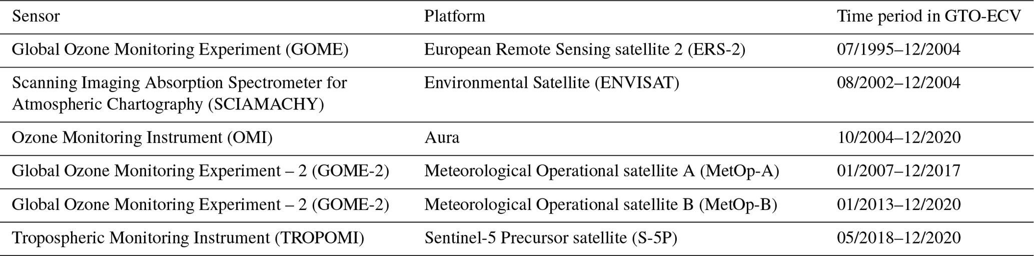
An overview of all satellite sensors included in GTO-ECV is given in Table 1. The third column shows the time period for which data from the respective sensor are incorporated in GTO-ECV. We use total ozone columns retrieved with the GOME Direct Fitting version 4 (GODFIT_V4) algorithm (Lerot et al., 2014; Garane et al., 2018), which is applied to all sensors. A full reprocessing of the entire time series of GOME, SCIAMACHY (Scanning Imaging Absorption Spectrometer for Atmospheric Chartography), OMI (Ozone Monitoring Instrument), and GOME-2A/-2B has been realized in the framework of the ESA-CCI and the EU-C3S ozone projects. Moreover, GODFIT is the baseline retrieval algorithm for the offline total ozone column products of TROPOMI/S-5P (Tropospheric Monitoring Instrument Sentinel-5 Precursor satellite), in addition to the GOME Data Processor (GDP) algorithm, which is used for the corresponding near-real-time products (Inness et al., 2019; Spurr et al., 2021).
Geophysical validation of the GODFIT_V4 level-2 total column ozone products from the individual nadir sensors with respect to ground-based reference instruments, such as Brewer, Dobson, and zenith-sky spectrometers, is evidence of its very good quality. The mean bias between the individual level-2 products and ground-based measurements is within 1.5 ± 1.0 % (Garane et al., 2018, 2019). Owing to the common retrieval algorithm the inter-sensor consistency of the selected instruments is overall extremely high (within 1.0 % between 50∘ N and 50∘ S; Garane et al., 2018). This is an excellent prerequisite for homogenizing and merging the individual time series, which is performed on daily gridded level-3 products that are generated from the corresponding level-2 products. In order to account for possible remaining biases and/or drifts between the individual data sets, adjustments are applied to GOME, SCIAMACHY, GOME-2A, GOME-2B, and TROPOMI, which all benefit from long overlap periods with OMI, whose measurements are used as a reference basis. The adjustments depend on latitude and time. Compared to the latest predecessor version of GTO-ECV, as described in Garane et al. (2018), TROPOMI has now been included as an additional sensor, and changes related to the time periods during which the individual sensors are used in GTO-ECV have been made (see Table 1 for the current time periods). For GOME we have extended the time period in order to improve the representativeness of GTO-ECV between 2003 and end of 2004, and for SCIAMACHY and GOME-2A we had to shorten the periods based on updated comparisons with the reference sensor OMI and ground-based measurements (Garane et al., 2018; Coldewey-Egbers et al., 2020).
The validation of GTO-ECV total ozone columns against ground-based observations reveals a very good overall agreement (i.e., similar to the validation of the level-2 data and with 0.5 % to 1.5 % peak-to-peak amplitude) and an excellent long-term stability (Garane et al., 2018). The drift with respect to ground-based data is well below 1 % per decade. Especially the negligible drift makes it useful for addressing open questions related to the evolution of the ozone layer, in particular to ozone recovery and interannual variability (Coldewey-Egbers et al., 2014; Chipperfield et al., 2018; Weber et al., 2018; Eleftheratos et al., 2019), or the evaluation of extreme values (Dameris et al., 2021).
The GTO-ECV data record is freely available from the Copernicus Climate Data Store (CDS; https://cds.climate.copernicus.eu, last access: 13 May 2022). It provides monthly mean total ozone columns, as well as the corresponding standard deviations and standard errors, from July 1995 through December 2020 on a spatial grid of in latitude and longitude in a user-friendly NetCDF format following the climate and forecast metadata conventions. Along with other long-term total ozone data records, GTO-ECV is used in relevant international assessments and reports such as the World Meteorological Organization (WMO) and United Nations Environment Programme (UNEP) Scientific Assessment of Ozone Depletion (e.g., Braesicke et al., 2018), the State of the Climate published as a supplement to the Bulletin of the American Meteorological Society (BAMS; e.g., Weber et al., 2021), and the Working Group I contribution to the Sixth Assessment Report of the Intergovernmental Panel on Climate Change (IPCC, 2021).
In this section, a brief description of the regression model that is used for trend estimation and a short summary of the selected explanatory variables are provided. We derive total ozone trends using a standard multivariate linear regression (MLR) model which is applied to deseasonalized monthly mean ozone anomalies obtained from the GTO-ECV data record. Please note that for trend analyses we converted the original product to a slightly larger grid size of 5∘ × 5∘. The MLR is used in the form given by
The equation quantifies the relationship between ozone anomalies and several explanatory variables describing natural forcings. ΔO3(m) is the deseasonalized ozone anomaly (in %), m is the number of months after the initial time, and a–g are the model fit coefficients calculated using a standard least squares algorithm. The sources and names of the selected explanatory variable time series are given in Table 2. Seasonal variability can be accounted for by expanding the respective coefficient like, for example, for the trend term (second term on the right hand side of Eq. 1):
where b0 is the annual mean trend. Depending on the choice of Nb it is possible to account for annual, semiannual, 4-month, and, if necessary, shorter-term variations. In our study, we include the seasonal variability only in the trend term but not in the other explanatory variables. We apply the MLR to the GTO-ECV product introduced in Sect. 2, but for trend estimation we use a slightly shorter time period from January 1997 through December 2020. The year 1997 is regarded as an adequate turnaround point for ozone in the middle latitudes after ODSs have peaked (Harris et al., 2008), and thus it should be an appropriate starting point for the investigation of the recovery period of ozone. However, the optimum inflection point may vary with latitude and altitude (SPARC/IO3C/GAW, 2019), and we have to keep in mind that trend estimates may be sensitive to the starting and end points of the regression (Harris et al., 2015).
Compared to the MLR used in Coldewey-Egbers et al. (2014), we added one more proxy, which is the Arctic Oscillation (AO) index, for all GTO-ECV grid cells in the Northern Hemisphere and the Antarctic Oscillation (AAO) index for all grid cells in the Southern Hemisphere in order to account for large-scale circulation processes in the middle latitudes (Reinsel et al., 2005; Steinbrecht et al., 2011; Weber et al., 2018). Moreover, we extended the latitude range for which we calculate the trend to 70∘ S–70∘ N. All covariates have been normalized to zero mean and unit variance, and the time series are shown in Fig. A1. A potential non-negligible autocovariance of the residuals X(m) is accounted for by applying a Cochrane–Orcutt transformation (Cochrane and Orcutt, 1949), and thus the regression is performed in an iterative procedure. In general, a fit coefficient is considered statistically significant when its absolute value is greater than 2 times its error (95 % confidence interval).
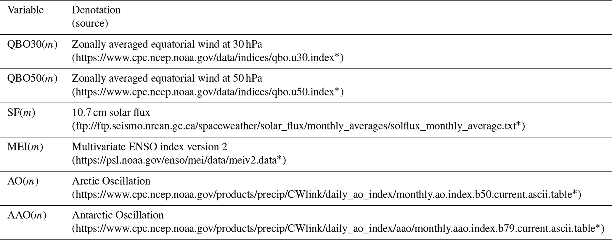
Table 2Sources of explanatory variable time series used in the MLR (Eq. 1). Figure A1 shows the time series (normalized to zero mean and unit variance) for all individual covariates.
* Last access: 13 May 2022
In general, between 70 % and 90 % of the ozone variance is explained by the full MLR as described in Eq. (1) when it is applied to total ozone columns (see also Coldewey-Egbers et al., 2014, their Fig. 2a). In the middle latitudes this variance is dominated to a large extent by the seasonal variability. In the tropics ozone variability is additionally induced by the QBO (quasi-biennial oscillation), the solar cycle, and ENSO (Toihir et al., 2018; Bencherif et al., 2020). Toward the high latitudes of the Southern Hemisphere the magnitude of the explained variance using our MLR decreases to about 50 %, suggesting that part of the forcing of ozone variability is missing in this region. In contrast to our model, in other ozone trend and variability studies the poleward heat flux is included as an additional and significant proxy (de Laat et al., 2015; Toro et al., 2017; Weber et al., 2018, 2022). This may explain the lower explained variance values we achieve with the MLR.
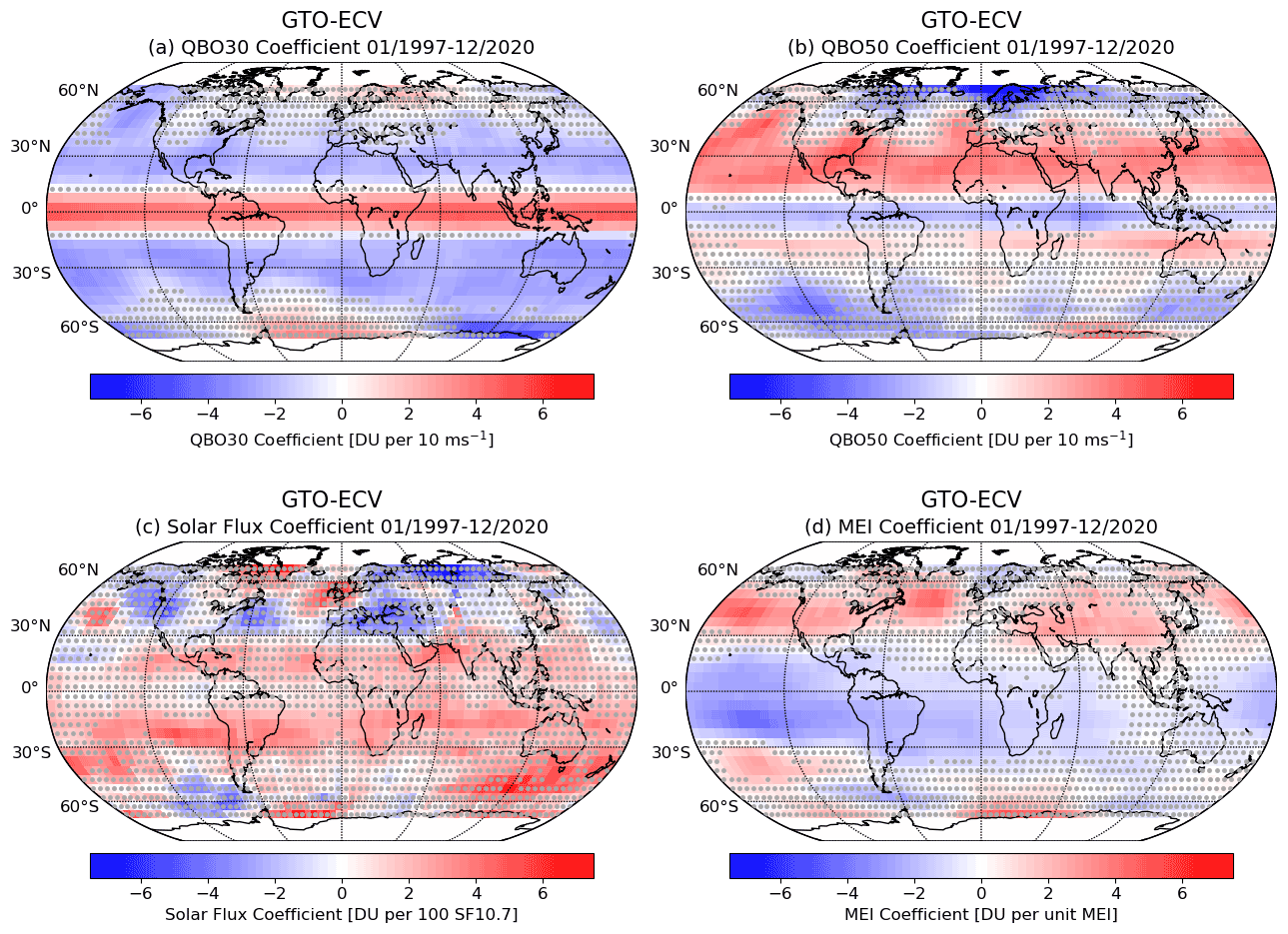
Figure 1MLR fit coefficients for the explanatory variables (a) QBO at 30 hPa (QBO30), (b) QBO at 50 hPa (QBO50), (c) solar flux (SF), and (d) multivariate ENSO index (MEI). The results are expressed in Dobson units (DU) per unit of the explanatory variable. Grey dots signify that the term is statistically not significant in this grid cell.
The QBO signal is approximated by both 30 and 50 hPa equatorial zonally averaged monthly winds denoted as QBO30(m) and QBO50(m) in Eq. (1). The QBO is the dominant source of stratospheric variability in the equatorial region (10∘ S–10∘ N), but it also has an impact in the subtropics (with the opposite sign) and to some extent in the middle latitudes (e.g., Steinbrecht et al., 2006; Frossard et al., 2013). The mean period is about 26–28 months. The QBO MLR fit coefficients c and d are shown in Fig. 1a and b. Additionally, the contribution of both proxies to ozone variability expressed in percent is shown in Fig. A2a and b. During the QBO's westerly phase there is a positive correlation between wind anomalies at 30 hPa and ozone and a negative correlation between wind anomalies at 50 hPa and ozone in the inner tropics. They are related to changes in up- and down-welling processes (Baldwin et al., 2001); i.e., the increase in ozone at 30 hPa is due to downward transport of ozone-rich air to altitudes where ozone lifetimes are relatively long.
In Eq. (1) SF(m) denotes the 10.7 cm radio flux and accounts for the impact of the 11-year solar cycle on ozone. Between solar activity and total ozone in the tropics, a positive correlation (though barely significant) exists which is shown in Fig. 1c. Enhanced ozone levels occur during solar maxima and vice versa. While the correlation pattern is basically zonally symmetric at low latitudes, it exhibits a longitudinal variance (though not statistically significant) at middle to high latitudes due to transport and dynamics (Steinbrecht et al., 2003; Coldewey-Egbers et al., 2014). However, an accurate quantification of the impact is difficult since only slightly more than two solar cycles are covered by GTO-ECV (see Fig. A1c). Moreover, the magnitude and timing of ozone variations in response to the solar cycle can be different from one cycle to the next (Steinbrecht et al., 2004). In general, the contribution of this proxy to ozone variability is below 10 % (see Fig. A2c).
The correlation between ozone and the ENSO pattern, which is represented by the multivariate ENSO index (MEI) and denoted by MEI(m) in Eq. (1), is negative for almost the entire tropics and has its maximum over the Pacific (see Fig. 1d). In this region the ozone variability explained by this variable is about 30 %–40 % (Fig. A2d). Significant changes in the convection pattern induced by El Niño or La Niña events lead to changes in tropospheric ozone amounts, whereas the stratospheric columns remain more or less unchanged. Cold (La Niña) events lead to an increase in tropospheric (and thus total) ozone mainly over the eastern Pacific due to reduced convection. On the other hand, warm (El Niño) events and enhanced convection lead to a decrease in ozone (Steinbrecht et al., 2006).

Figure 2(a) MLR fit coefficient for the additional explanatory variables AO (applied in Northern Hemisphere) and AAO (applied in the Southern Hemisphere) in Dobson units (DU) per unit (A)AO index. (b) Difference in explained variance (in %) between the MLR including the A(AO) proxy and the MLR without the additional proxy.
Figure 2a shows the fit coefficient for the Arctic Oscillation (AO) index (applied in the Northern Hemisphere only) and the Antarctic Oscillation (AAO) index (applied in the Southern Hemisphere only). In the Northern Hemisphere the correlation is significant mainly over the eastern part of North America, the Atlantic Ocean, Europe, and over Eurasia. The observed pattern over the North Atlantic sector suggests a strong correlation with the North Atlantic Oscillation (NAO) pattern which is a part of the AO. During the positive phase of the AO (or the NAO) the pressure gradient between the Icelandic Low and the Azores High is stronger than normal, i.e., lower than normal pressure in the north and higher than normal pressure further south. The corresponding lower tropopause altitude leads to an increase in total ozone (i.e., a positive correlation between AO and ozone, which is centered over the Labrador Sea), whereas further south a higher than normal tropopause altitude leads to a decrease in total ozone, i.e., a negative correlation (cf. Appenzeller et al., 2000; Rieder et al., 2010; Steinbrecht et al., 2011; Zhang et al., 2017). Over Eurasia, poleward of 40∘ N, the correlation is significantly negative; i.e., ozone is lower during the positive phase of the AO. The positive phase of the AO is related to a strengthened polar vortex, lower than normal air pressure, and enhanced ozone depletion over high latitudes (Liu and Hu, 2021). According to Thompson and Wallace (1998) and Zou et al. (2005) this correlation is more pronounced over Eurasia than over the North Atlantic region. Thompson and Wallace (2000, their Fig. 12) also stated that the area of a negative correlation between AO and ozone reaches from the polar cap to 40∘ N, which is in good agreement with Fig. 2a. The zonal asymmetry in the correlation indicating a positive maximum over the Labrador Sea is reproduced as well. The positive correlation between AO and ozone in the tropics is probably related to a lowering of the tropopause in conjunction with temperature changes (Thompson and Wallace, 2000). For the Southern Hemisphere and the corresponding AAO a similar relationship as for the AO was found. Ozone is reduced during the positive phase of the AAO from 60∘ W to 120∘ E. The zonal asymmetry found by Thompson and Wallace (2000) expressed by a positive correlation northwest of the Antarctic Peninsula is reproduced, but in the region south of Australia, we see a discrepancy between our results (slightly positive correlation) and their findings (negative correlation).
Figure 2b shows the difference in the explained variance between the new MLR including the (A)AO proxies and the old model without (A)AO proxies. The explained variance is enhanced in those regions discussed above which show a significant correlation with total ozone. In the Northern Hemisphere a maximum increase of 15 %–17 % is found in the 55–60∘ N latitude belt around 60∘ W and poleward of 45∘ N from 90 to 150∘ E. In the Southern Hemisphere we found an increase of ∼ 9 % in the latitude range 45–60∘ S from 60∘ W to 90∘ E. Note that we do not expect significant changes regarding the ozone trend and its spatial pattern when we include the additional terms in the MLR, but uncertainty should be further reduced (see also Weber et al., 2018). However, small changes in the trend might be observed as a response to a possible positive long-term drift in the additional dynamical proxies (cf. Weber et al., 2022). Moreover, Fig. A1e also indicates that toward the end of the time period (2013–2020) the AO was mainly in its positive phase (Hu et al., 2018).
4.1 Annual mean trends
The annual mean total ozone trend in percent per decade derived from the GTO-ECV data record for the time period 1997–2020 and the latitude range 70∘ S–70∘ N is shown in Fig. 3. The MLR (Eq. 1) has been applied to all 5∘ × 5∘ grid cells separately, and grey dots signify that the trend in a grid cell is statistically not significant at the 2σ uncertainty level.
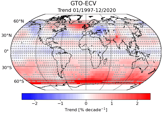
Figure 3Total ozone trend for 1997–2020 (in % per decade) derived from the GTO-ECV data record. Grey dots signify that the trend is statistically not significant at the 2σ uncertainty level.
In the middle latitudes of the Northern Hemisphere the trend indicates a longitudinal structure, although the trend is statistically not significant for almost the entire latitude band. The zonal average of the trends is close to zero and not significant. Small regions which show significant trends are the North Atlantic between 50 and 60∘ N, as well as eastern Europe and the Black Sea. Over the northern Atlantic the trend is positive ( per decade), and over eastern Europe and the Black Sea the trend is negative ( per decade). Note that all uncertainties are reported as 2σ. A similar spatial pattern was found by Sofieva et al. (2021, their Fig. 10) and by Arosio et al. (2019). Their height-resolved trends also indicate in the Northern Hemisphere a longitudinal dependence. Positive trends were found over Scandinavia and the North Atlantic at almost all altitudes. They are statistically significant in the upper stratosphere above 40 km. Non-significant negative trends were found by Sofieva et al. (2021) below 40 km in the same regions as found here for the total column, i.e., in the northern Pacific, the Atlantic (30–45∘ N), and over eastern Europe and the Black Sea. These longitudinal structures suggest that the trends seem to have non-negligible contributions from dynamical and climate change effects (Zhang et al., 2018, 2019; Sofieva et al., 2021), which cannot be easily separated from the ODS-related trends considering the explanatory variables used in this study. The spatial trend pattern in the Northern Hemisphere described above indicates some positive correlation with the fit coefficient for the AO proxy (Fig. 2a). Since changes in ozone related to this forcing are at least partly induced by changes in tropopause altitude, we investigate this relationship later in this section in more detail. The significant positive trend we found north of India is mainly caused by artificial outliers in the GTO-ECV data record. This region is impacted by regular data gaps in the GOME/ERS-2 time series (see also https://atmos.eoc.dlr.de/app/calendar, last access: 13 May 2022) and should be omitted for the analysis and interpretation of ozone trends.
In the tropics the trend does not show a noticeable longitudinal variation. Moreover, it is not significant from 30∘ N to 20∘ S, which is in good agreement with Braesicke et al. (2018). It is assumed that the total ozone trend in this region is governed by various dynamical and chemical processes at different altitudes competing with each other. In particular, an increase in ozone is expected in both the troposphere and the upper stratosphere. An increase in the troposphere is most probably due to changes in surface emissions of precursor constituents, and the increase in the upper stratosphere is expected to be related to both decreasing amounts of ODSs and an increase in greenhouse gases. The latter leads to a cooling which will in turn lead to an increase in ozone levels (Meul et al., 2016; Keeble et al., 2017; Toihir et al., 2018). On the other hand, changes in the tropical lower stratosphere are governed by transport processes. A negative trend in ozone due to an enhanced Brewer–Dobson circulation (BDC) as a consequence of increasing amounts of greenhouse gases is expected and has already been detected (Eyring et al., 2010; Ball et al., 2018, 2019; Szeląg et al., 2020).
Southward of 20∘ S some regions indicate significant positive trends, mainly in the Pacific, south of Africa, and around Australia. Almost 45 % of all grid cells between 30 and 70∘ S exhibit significant trends. The positive trend increases from 0.6±0.5 % per decade in the southern subtropics to 1.0±0.9 % per decade in the middle latitudes and 2.8±2.6 % per decade in the latitude band 60–70∘ S.
The latitudinal structure of the estimated trends is quite similar to the results described in Weber et al. (2022), who analyzed annual mean zonal mean data from different data sets (one of which was GTO-ECV) for the period 1979–2020. In their paper significant positive trends in zonal mean ozone of about 0.6 %–1.0 % per decade were detected in the middle latitudes of the Southern Hemisphere, whereas they were insignificant in the tropics and barely significant (0.5 ± 0.5 % per decade) in the Northern Hemisphere middle latitudes.
When we compare our new results derived for the annual mean ozone trend using the extended (by 7.5 years and additional satellite sensors) GTO-ECV data record, as well as an expanded MLR (Fig. 3), with the findings from Coldewey-Egbers et al. (2014, their Fig. 1a), we notice that the overall spatial pattern changed, in particular in the tropical region and in the Southern Hemisphere. The significant positive trend which we identified in the previous study for the tropics and which was attributed mainly to the impact of changes in ENSO intensity is now insignificant for the entire region (except for the southern subtropics of 20–30∘ S). On the other hand, in the middle latitudes of the Southern Hemisphere we now find significant positive trends. In the middle latitudes of the Northern Hemisphere the spatial pattern remains more or less the same. Significant positive trends over the North Atlantic region and (non-significant) negative trends elsewhere were already found in the predecessor study.
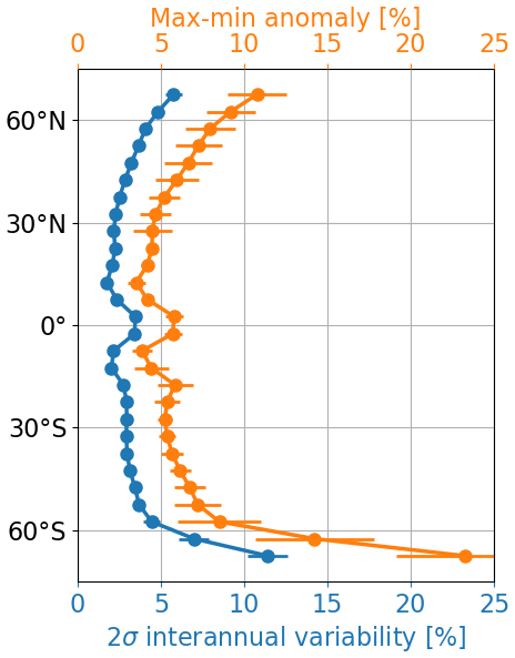
Figure 4Interannual variability (%) in total ozone as a function of latitude derived from the GTO-ECV data record. The blue curve signifies 2 times the standard deviation of the yearly ozone anomalies based on the reference period 1997–2020, and the orange curve signifies the corresponding range (maximum–minimum) of the anomaly. The error bars signify the variation in the variability with longitude.
In the Southern Hemisphere extratropical region it seems that the expected positive ozone trend related to decreasing amounts of ODSs becomes more evident. The trend does not indicate a significant longitudinal structure as found in the Northern Hemisphere or an apparent correlation with the AAO proxy. On the other hand, in the Northern Hemisphere it seems that the expected ODS-related trend is compensated for or masked by trends induced by other, for example, dynamical factors (Weber et al., 2022). On top of that, the year-to-year variability in ozone in the middle and high latitudes is quite strong (Weber et al., 2018; Braesicke et al., 2018; SPARC/IO3C/GAW, 2019). For an illustration, Fig. 4 shows the interannual variability in total ozone derived from the GTO-ECV data record during the period 1997–2020. As a measure for interannual variability (blue curve) we take 2 times the standard deviation of the yearly ozone anomalies based on the reference period 1997–2020. The error bars signify the variation in the variability with longitude. The variability is around 2 % in the subtropics. Toward the middle and high latitudes it increases to ∼ 5 % (see also Braesicke et al., 2018). It is maximum (up to 10 %) in the Southern Hemisphere, mainly determined by the year-to-year variation in the Antarctic ozone hole. There is a small local maximum in the inner tropics related to the regular QBO variations. The orange curve signifies the range (maximum minus minimum) of the yearly anomalies, which is between 10 % in the Northern Hemisphere (60–70∘ N), 5 % in the tropics, and 20 % in the Southern Hemisphere (60–70∘ S). The numbers retrieved for the interannual variability in total ozone underpin the challenge regarding the detection of expected ozone trends of the order of ∼ 1 %–2 % relative to the year-to-year variation of ∼ 5 % in the middle latitudes.
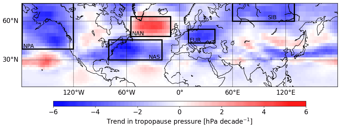
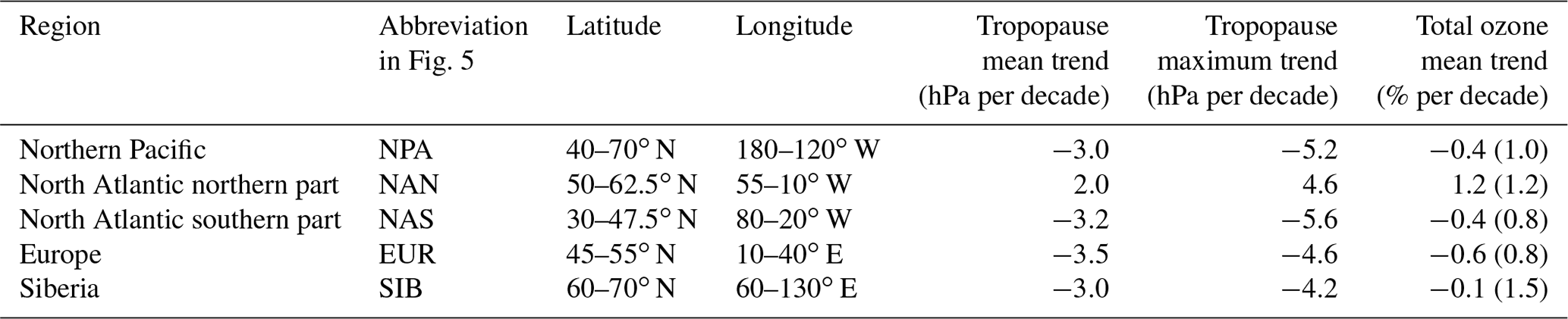
Figure 5Linear trend for 1997–2020 in tropopause pressure (hPa per decade) derived from the NCEP/NCAR (National Center for Atmospheric Research) reanalysis data. Black rectangles signify five regions for which we provide the mean and maximum trends in Table 3. These regions are the northern Pacific (NPA), the northern part of the North Atlantic (NAN), the southern part of the North Atlantic (NAS), Europe (EUR), and Siberia (SIB).
As mentioned earlier, the spatial pattern of the ozone trend in the middle latitudes of the Northern Hemisphere indicates a correlation with the AO proxy. In order to elaborate on this in more detail, we apply a simple linear regression to a tropopause altitude data product for the period 1997–2020. On a global scale, the trend in tropopause altitude is positive over recent decades and primarily thermally driven due to warming of the troposphere as a consequence of increasing amounts of greenhouse gases (Santer et al., 2003a, b; Pisoft et al., 2021). However, some notable latitudinal and longitudinal variation in the tropopause altitude trend, as well as upward/downward trend dipoles, was found (Xian and Homeyer, 2019). Since we do not see an apparent correlation between the spatial pattern of the ozone trend and the AAO proxy in the Southern Hemisphere, we limit our analysis to the Northern Hemisphere (0–70∘ N). We use the NCEP (National Centers for Environmental Prediction) reanalysis-derived tropopause altitude data product (i.e., monthly mean values on a regular grid of 2.5∘ × 2.5∘ in latitude and longitude) that is provided by the National Oceanic and Atmospheric Administration, Oceanic and Atmospheric Research, and Earth System Research Laboratories (NOAA/OAR/ESRL) Physical Science Laboratory (PSL) in Boulder, Colorado, USA (Kalnay et al., 1996).
The estimated linear trend for the tropopause pressure is shown in Fig. 5. In addition, Table 3 shows the mean and the maximum values of the trend in tropopause pressure calculated in five selected regions (northern Pacific, North Atlantic northern and southern parts, Europe, and Siberia), which are marked by the black rectangles in Fig. 5. In addition, the last column of Table 3 shows the corresponding mean trend in total ozone. For the northern Pacific, for both the southern and northern parts of the North Atlantic, and for Europe, we find positive correlations with the trend in ozone. The regions indicating a negative trend in ozone (see Fig. 3) also show a negative trend in tropopause pressure between −3.0 and −3.5 hPa per decade. The negative pressure trend corresponds to an increase of about 100–130 m per decade in tropopause height. On the other hand, the northern part of the North Atlantic (NAN) indicates a positive trend both in ozone (1.2 ± 1.2 % per decade) and in tropopause pressure. The latter is about 2 hPa per decade in that region.
The positive correlation between tropopause pressure and total ozone has been described in, for example, Hoinka et al. (1996), Steinbrecht et al. (1998), and Varotsos et al. (2004). Short-term and long-term variations in ozone have been associated with changes in tropopause height. For the European station Hohenpeißenberg it was found that about 25 % of the negative long-term trend in total ozone could be attributed to a tropopause that moved up by 150 ± 70 m per decade (Steinbrecht et al., 1998). However, longitudinal and latitudinal variation in the relation between both variables was observed (Varotsos et al., 2004). Because of the apparent correlation we conclude that the spatial pattern in the ozone trend (Fig. 3) is at least partly induced by changes in tropopause altitude that vary with latitude and longitude. However, over Siberia the correlation between the trend in tropopause and ozone is less clear. The trend in total ozone is very close to zero (−0.1 ± 1.5 % per decade), whereas the change in tropopause pressure is about −3.0 hPa per decade.
Table 3Average and maximum linear trends in tropopause pressure (in hPa per decade), as well as average linear trend in total ozone and corresponding 2σ uncertainty (in parenthesis; in % per decade) for five selected regions in the Northern Hemisphere (see also Fig. 5, black rectangles).
4.2 Seasonal dependence of trends
The seasonal dependence of the total ozone trend obtained from the gridded GTO-ECV data record is shown in Fig. 6. It has been determined by expanding the fit coefficient for the trend as described in Eq. (2). In general, the spatial pattern of the trend in each season is very similar to the pattern of the annual mean trend (see Fig. 3), and latitudinal and longitudinal structures do not change substantially in the course of the year. On a global scale, clear and significant seasonal variations are not visible.
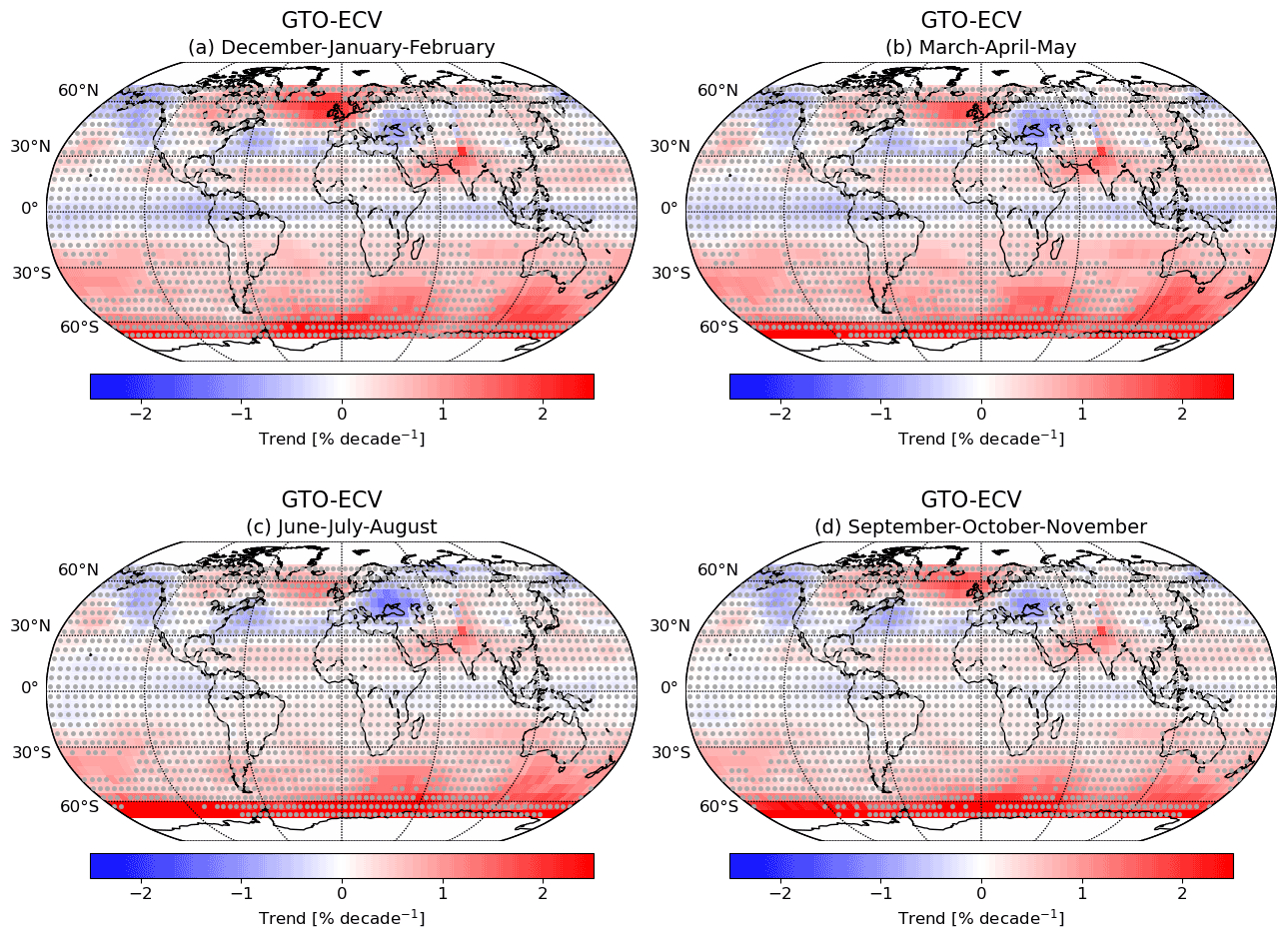
Figure 6Total ozone trend for 1997–2020 (in % per decade) derived from the GTO-ECV data record as a function of season: (a) December, January, February (DJF), (b) March, April, May (MAM), (c) June, July, August (JJA), and (d) September, October, November (SON). Grey dots signify that the trend is statistically not significant.
However, small seasonal changes are found in the Northern Hemisphere in the North Atlantic region and over eastern Europe. In the North Atlantic region between 45 and 70∘ N we note that the significant positive trend is most pronounced between December and February. This is in agreement with Szeląg et al. (2020, their Fig. 4); they analyzed zonal mean trends and found positive trends mainly in the upper stratosphere with a maximum in local winter. Additionally, our results using the gridded data set reveal that over the eastern part of Europe the trend is negative and significant for a small region between 40 and 50∘ N and 30 and 50∘ E (see also Fig. 3). Contrary to the positive trend over the North Atlantic, the negative trend is most pronounced from June to August (Fig. 6c). Moreover, this seasonal pattern agrees with the general conclusion of Bozhkova et al. (2019), who analyzed ozone trends in the middle latitudes of the Northern Hemisphere and found an overall increase in winter and a continuing decrease in summer for the period 2000–2017. The seasonal pattern we observed in this latitude band could be related to meridional transport processes that are controlled by the wave-driven BDC. The BDC is most active in local winter (Butchart et al., 2006), and a strengthening and acceleration of the BDC are prevalent in these months as well (Li et al., 2008). In the previous section we described the correlation of the spatial pattern of the annual mean ozone trend in the Northern Hemisphere with the linear trend in tropopause pressure. Note that there is no corresponding seasonal pattern in the tropopause pressure.
In the tropical region (30∘ N–20∘ S) total ozone trends are not significant throughout the whole year. This is probably caused by the quite variable and ambiguous seasonal and altitude dependence of the ozone trends in this region (Szeląg et al., 2020). The equatorial band 10∘ S–10∘ N indicates non-significant negative trends which are most pronounced from March to May and which are possibly governed by seasonal variation in the lower stratosphere (Szeląg et al., 2020).
In the extratropical region of the Southern Hemisphere significant positive trends are found throughout the whole year. However, in the middle latitudes (35–50∘ S) the positive trends found in the Pacific, south of southern Africa, and south of Australia are strongest between March and May. Further south, in the latitude range 55–70∘ S the positive trend, which is significant over the southern Pacific (110–180∘ W) and around 0∘ E/W (see Fig. 6), is most pronounced in austral winter, i.e., between June and August (cf. Szeląg et al., 2020, their Fig. 4). As for the Northern Hemisphere, this pattern could be related to the seasonal dependence of meridional transport processes.
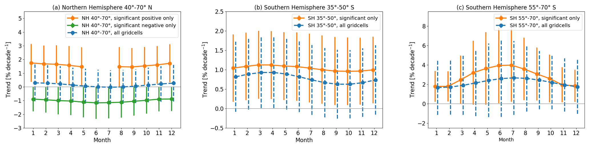
Figure 7Total ozone trend as a function of month for three different latitude bands: (a) Northern Hemisphere 40–70∘ N, (b) Southern Hemisphere 35–50∘ S, and (c) Southern Hemisphere 55–70∘ S.
For a more detailed illustration of the seasonal dependence we investigate the trend in three latitude bands – 40–70∘ N, 35–50∘ S, and 55–70∘ S – for which we found significant trends in total ozone columns at least for some regions. Figure 7 shows the trend as a function of month for the three selected zonal bands. The trend is shown averaged over all grid cells in this band (dashed blue curves), averaged over all grid cells which indicate significant positive trends (solid orange curves), and, in the case of the Northern Hemisphere, averaged over all grid cells indicating a significant negative trend (solid green curve in Fig. 7a). Hence, the orange and the green curves represent the seasonal behavior of the trend only for some longitudes in the respective latitude band. The observed seasonal variation is not significant, neither for all grid cells in the latitude band (blue curves) nor for the grid cells, indicating statistically significant trends (orange and green curves), as indicated by the corresponding error bars in Fig. 7.
In the middle latitudes of the Northern Hemisphere (Fig. 7a) the positive trend is maximum in boreal winter from December to March, although the seasonal variation is very small (±0.1 %) and not significant. The average positive trend (solid orange line), which comes mostly from grid cells in the North Atlantic region, is ∼ 1.7 % per decade, and the mean negative trend (solid green line, mostly from grid cells in the eastern part of Europe) is about −1.1 % per decade. If the estimated trends from all grid cells in this band are averaged (dashed blue curve), the trend is close to zero and not significant, which is in line with studies analyzing zonal mean ozone data records, e.g., Weber et al. (2018).
In the middle latitudes of the Southern Hemisphere (35–50∘ S, Fig. 7b) the trend is ∼ 1.0 % per decade in those regions, indicating a significant positive trend, and the maximum occurs between March and May. During these months the corresponding zonal mean trend (all grid cells) is also on the edge of being significant (dashed blue curve). Figure 7c shows the seasonal variation in the trend in the band 55–70∘ S. The trend itself and the seasonal variation are much larger compared to the other bands. For the grid cells indicating a significant positive trend it varies from +2 % per decade (December to February, local summer) to +4.0 % per decade in local winter from June to August. Although the trend is found to be maximum in July, the clarity of the significance of the positive trend in this zonal band is higher in August (3.6 ± 3.2 % per decade) and September (3.1 ± 2.7 % per decade). Significant positive trends in September and a strong seasonality were also found in Antarctica (63–90∘ S) by, for example, Solomon et al. (2016, 2017) and Kuttippurath and Nair (2017). Contrary to our results these studies indicate a maximum trend between September and December, whereas the minimum occurs from May to July. Note that our results cover only the latitude band 55–70∘ S and consider only the longitude regions where the trend is significant and are thus not representative for the entire polar cap like the aforementioned studies. Moreover, these studies also used high-resolution ozonesonde data, which might explain the discrepancy. On top of that, this latitude band is significantly affected by the limited coverage of the satellite data during local winter from June to August, and the results in these months should be interpreted with great care.
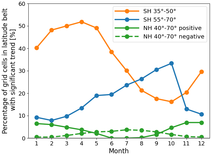
Figure 8Percentage of grid cells indicating a significant trend as a function of month for the latitude bands 40–70∘ N (green), 35–50∘ S (orange), and 55–70∘ S (blue). The number is provided in percent of the total number of grid cells in the respective band. For the Northern Hemisphere (green) a division between significant positive (solid curve) and significant negative (dashed curve) trends is made.
To further illustrate and underpin the observed seasonal variation, Fig. 8 shows the percentage of grid cells which indicate significant trends in the respective latitude band. The zonal bands and time periods showing the largest percentage of significant positive trends in total ozone are March and April in the middle latitudes of the Southern Hemisphere (50 %–55 %) and September to October in the band 55–70∘ S (∼ 30 %). The percentage of grid cells indicating significant trends in the Northern Hemisphere (green curves) is much smaller compared to the Southern Hemisphere but is similar for positive trends from December to February, when about 10 % of the grid cells indicate a positive trend. For the negative trend in the Northern Hemisphere the maximum percentage occurs from June to August, but it is well below 10 %. As seen in Figs. 3 and 6 the regions showing significant trends in the Northern Hemisphere are limited to the North Atlantic sector and the southeastern part of Europe.
In this work we present an updated and detailed perspective on near-global (70∘ N–70∘ S) total ozone trends for the last quarter century. We use the GTO-ECV data record which has been extended and generated in the framework of the ESA-CCI and EU-C3S ozone projects. GTO-ECV combines total ozone observations from six nadir-viewing satellite sensors of the GOME type. The latest addition was the data record of the TROPOMI instrument launched in October 2017. GTO-ECV covers the period from July 1995 through December 2020 and provides an excellent spatial resolution of 1∘ × 1∘.
The key aspect of our study is the analysis of latitudinally and longitudinally resolved patterns of the ozone trend, as well as the investigation of its seasonal dependence. We evaluate the linear trend using a standard MLR method including several explanatory variables such as the quasi-biennial oscillation, the solar cycle, El Niño–Southern Oscillation, and Arctic and Antarctic oscillations.
In the Southern Hemisphere we found statistically significant positive trends that increase from 0.6 ± 0.5 % per decade in the subtropics to 1.0 ± 0.9 % per decade in the middle latitudes and 2.8 ± 2.6 % per decade in the latitude band 60–70∘ S. In the middle latitudes of the Northern Hemisphere the trend exhibits distinct regional patterns, i.e., latitudinal and longitudinal structures. Significant positive trends (∼ 1.5 ± 1.0 % per decade) over the North Atlantic region, as well as negative trends (−1.0 ± 1.0 % per decade) over eastern Europe, were found. The northern Pacific indicates non-significant negative trends. Furthermore, these trends exhibit a correlation with long-term changes in tropopause pressure (see also Zhang et al., 2019). The hemispheric differences indicate that in the Northern Hemisphere the ozone trend is determined by both dynamic and ODS-related effects, which may induce changes of opposite signs, while in the Southern Hemisphere the less pronounced longitudinal structures in the overall positive trends may suggest that ODS-related effects prevail, which is in good agreement with Weber et al. (2022). Total ozone trends in the tropics are not statistically significant, which is most likely a result of opposed trends at different altitudes in the troposphere and stratosphere (Meul et al., 2016; Szeląg et al., 2020).
Regarding the seasonal dependence of the trends we found only very small non-significant variations over the course of the year. However, we identified different behavior depending on latitude. In the latitude band 40–70∘ N the positive trend maximizes in boreal winter from December to February. In the middle latitudes of the Southern Hemisphere (35–50∘ S) the trend is maximum from March to May. Further south toward the high latitudes (55–70∘ S) the trend exhibits a relatively strong seasonal cycle which varies from ∼ 2 % per decade in December and January to ∼ 3.8 % per decade in June and July (austral winter). The clarity of the significance in this band is maximum in August and September. The non-significant maxima in local winters in both hemispheres might be related to the impact of the meridional transport of ozone (and other trace gases) that is controlled by the Brewer–Dobson circulation. An acceleration of the BDC due to increasing amounts of greenhouse gases is expected (Butchart et al., 2006; Braesicke et al., 2003), which might induce the observed seasonal behavior but also contribute to long-term changes in ozone in addition to ODS-related increases (Harris et al., 2008; Weber et al., 2022).
Our study shows that continued monitoring of the ozone layer and further extension of high-quality ozone data records, which provide reliable information about the temporal evolution and spatial variability, are needed. This will enable us to improve our current understanding of past changes in ozone and to gain more confidence in the attribution of the trends to various processes. Moreover, various other total ozone data sets such as chemistry–climate model simulations, re-analysis data, or similar satellite-based records could benefit from a comparison with GTO-ECV in order either to assess the capability of the models' systems or to identify drawbacks, e.g., jumps or drifts in one of the satellite-based records (see, e.g., Loyola et al., 2009; Chiou et al., 2014; Coldewey-Egbers et al., 2020).
Figure A1 shows the time series 1997–2020 of all explanatory variables used in the MLR (Eq. 1) normalized to zero mean and unit variance. Black curves in (e) and (f) signify a 3-month running mean. Figure A2 shows the contributions of the individual explanatory variables QBO30 (a), QBO50 (b), solar flux (c), and MEI (d) to the ozone variability, expressed in percent. The contribution of the (A)AO proxy is shown in Fig. 2b.
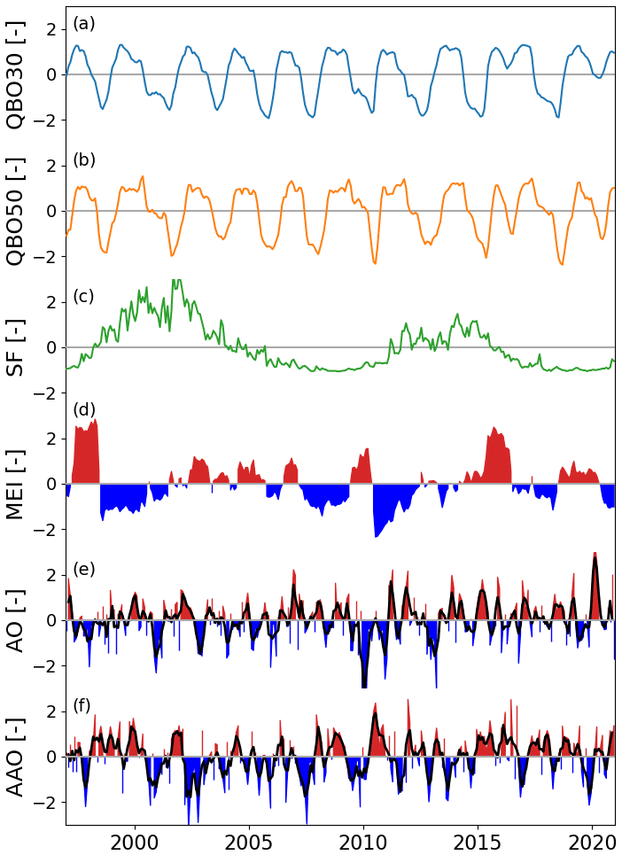
Figure A1Time series 1997–2020 of all explanatory variables used in the MLR (Eq. 1) normalized to zero mean and unit variance: (a) QBO30, (b) QBO50, (c) SF, (d) MEI, (e) AO, and (f) AAO. Black curves in (e) and (f) signify a 3-month running mean.
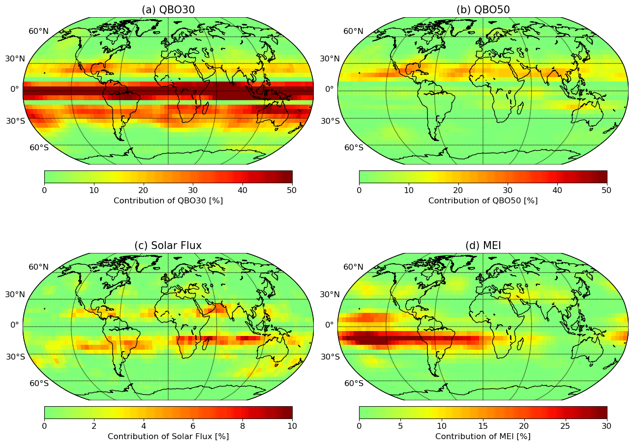
Figure A2Contributions of the individual explanatory variables (a) QBO30, (b) QBO50, (c) solar flux, and (d) MEI to ozone variability, expressed in percent.
The GTO-ECV data record is publicly available via the Copernicus Climate Data Store (https://doi.org/10.24381/cds.4ebfe4eb, Coldewey-Egbers and Loyola, 2020). The level-2 ozone products from GOME, SCIAMACHY, OMI, and GOME-2 are available on the Ozone_CCI ftp site at the following address: ftp://cci_web@ftp-ae.oma.be/esacci (DOIs: https://doi.org/10.18758/71021038, Lerot, 2022a; https://doi.org/10.18758/71021037, Lerot, 2022b; https://doi.org/10.18758/71021036, Lerot, 2022c; https://doi.org/10.18758/71021034, Lerot, 2022d; https://doi.org/10.18758/71021035, Lerot, 2022e). The TROPOMI GODFIT ozone products are publicly available on the Copernicus Sentinel-5P data hub (https://doi.org/10.5270/S5P-ft13p57, European Space Agency, 2020).
MCE and DGL were responsible for the generation of the GTO-ECV data record. MCE performed the trend analysis, and CL and MVR were responsible for the generation of level-2 ozone data records. All authors contributed to the revision of the manuscript.
At least one of the (co-)authors is a member of the editorial board of Atmospheric Chemistry and Physics. The peer-review process was guided by an independent editor, and the authors also have no other competing interests to declare.
Publisher’s note: Copernicus Publications remains neutral with regard to jurisdictional claims in published maps and institutional affiliations.
This article is part of the special issue “Atmospheric ozone and related species in the early 2020s: latest results and trends (ACP/AMT inter-journal SI)”. It is a result of the 2021 Quadrennial Ozone Symposium (QOS) held online on 3–9 October 2021.
NCEP reanalysis-derived data were provided by the NOAA/OAR/ESRL PSL, Boulder, Colorado, USA. We thank EU/ESA/DLR/BIRA-IASB for providing the TROPOMI/S5P Level-2 ozone products; this paper contains modified Copernicus data (2018/2020) processed by DLR. The GTO-ECV data used in this work were developed and generated in the framework of the ESA CCI+ and EU-C3S projects.
Melanie Coldewey-Egbers and Diego G. Loyola were supported by the DLR projects MABAK and INPULS.
The article processing charges for this open-access publication were covered by the German Aerospace Center (DLR).
This paper was edited by Jayanarayanan Kuttippurath and reviewed by three anonymous referees.
Appenzeller, C., Weiss, A. K., and Staehelin, J.: North Atlantic Oscillation modulates total ozone winter trends, Geophys. Res. Lett., 27, 1131–1134, https://doi.org/10.1029/1999GL010854, 2000. a
Arosio, C., Rozanov, A., Malinina, E., Weber, M., and Burrows, J. P.: Merging of ozone profiles from SCIAMACHY, OMPS and SAGE II observations to study stratospheric ozone changes, Atmos. Meas. Tech., 12, 2423–2444, https://doi.org/10.5194/amt-12-2423-2019, 2019. a, b, c
Baldwin, M. P., Gray, L. J., Dunkerton, T. J., Hamilton, K., Haynes, P. H., Randel, W. J., Holton, J. R., Alexander, M. J., Hirota, I., Horinouchi, T., Jones, D. B. A., Kinnersley, J. S., Marquardt, C., Sato, K., and Takahashi, M.: The Quasi-Biennial Oscillation, Rev. Geophys., 39, 179–229, 2001. a
Ball, W. T., Alsing, J., Mortlock, D. J., Staehelin, J., Haigh, J. D., Peter, T., Tummon, F., Stübi, R., Stenke, A., Anderson, J., Bourassa, A., Davis, S. M., Degenstein, D., Frith, S., Froidevaux, L., Roth, C., Sofieva, V., Wang, R., Wild, J., Yu, P., Ziemke, J. R., and Rozanov, E. V.: Evidence for a continuous decline in lower stratospheric ozone offsetting ozone layer recovery, Atmos. Chem. Phys., 18, 1379–1394, https://doi.org/10.5194/acp-18-1379-2018, 2018. a, b, c
Ball, W. T., Alsing, J., Staehelin, J., Davis, S. M., Froidevaux, L., and Peter, T.: Stratospheric ozone trends for 1985–2018: sensitivity to recent large variability, Atmos. Chem. Phys., 19, 12731–12748, https://doi.org/10.5194/acp-19-12731-2019, 2019. a, b, c
Ball, W. T., Chiodo, G., Abalos, M., Alsing, J., and Stenke, A.: Inconsistencies between chemistry–climate models and observed lower stratospheric ozone trends since 1998, Atmos. Chem. Phys., 20, 9737–9752, https://doi.org/10.5194/acp-20-9737-2020, 2020. a
Bencherif, H., Toihir, A. M., Mbatha, N., Sivakumar, V., du Preez, D. J., Bègue, N., and Coetzee, G.: Ozone Variability and Trend Estimates from 20-Years of Ground-Based and Satellite Observations at Irene Station, South Africa, Atmosphere, 11, 1216, https://doi.org/10.3390/atmos11111216, 2020. a
Bozhkova, V., Liudchik, A., and Umreiko, S.: Long-term trends of total ozone content over mid-latitudes of the Northern Hemisphere, Int. J. Remote Sens., 40, 5216–5229, https://doi.org/10.1080/01431161.2019.1579384, 2019. a
Braesicke, P., Jrrar, A., Hadjinicolaou, P., and Pyle, J.: Variability of total ozone due to the NAO as represented in two different model systems, Meteorol. Z., 12, 203–208, https://doi.org/10.1127/0941-2948/2003/0012-0203, 2003. a
Braesicke, P., Neu, J., Fioletov, V., Godin-Beekmann, S., Hubert, D., Petropavlovskikh, I., Shiotani, M., and Sinnhuber, B.-M.: Update on Global Ozone: Past, Present, and Future, Chapter 3, Scientific Assessment of Ozone Depletion: 2018, Global Ozone Research and Monitoring Project – Report No. 58, World Meteorological Organization, Geneva, Switzerland, https://ozone.unep.org/sites/default/files/2019-05/SAP-2018-Assessment-report.pdf (last access: 20 May 2022), 2018. a, b, c, d, e, f, g, h, i, j
Butchart, N., Scaife, A. A., Bourqui, M., de Grandpré, J., Hare, S. H. E., Kettleborough, J., Langematz, U., Manzini, E., Sassi, F., Shibata, K., Shindell, D., and Sigmond, M.: Simulations of anthropogenic change in the strength of the Brewer–Dobson circulation, Clim. Dynam., 27, 727–741, https://doi.org/10.1007/s00382-006-0162-4, 2006. a, b
Chiou, E. W., Bhartia, P. K., McPeters, R. D., Loyola, D. G., Coldewey-Egbers, M., Fioletov, V. E., Van Roozendael, M., Spurr, R., Lerot, C., and Frith, S. M.: Comparison of profile total ozone from SBUV (v8.6) with GOME-type and ground-based total ozone for a 16-year period (1996 to 2011), Atmos. Meas. Tech., 7, 1681–1692, https://doi.org/10.5194/amt-7-1681-2014, 2014. a
Chipperfield, M. P., Dhomse, S., Hossaini, R., Feng, W., Santee, M. L., Weber, M., Burrows, J. P., Wild, J. D., Loyola, D., and Coldewey-Egbers, M.: On the Cause of Recent Variations in Lower Stratospheric Ozone, Geophys. Res. Lett., 45, 5718–5726, https://doi.org/10.1029/2018GL078071, 2018. a, b
Cochrane, D. and Orcutt, G. H.: Application of Least Squares Regression to Relationships Containing Auto-Correlated Error Terms, J. Am. Stat. Assoc., 44, 32–61, https://doi.org/10.1080/01621459.1949.10483290, 1949. a
Coldewey-Egbers, M. and Loyola, D. G.: GOME-type Total Ozone Essential Climate Variable (GTO-ECV), C3S [data set], https://doi.org/10.24381/cds.4ebfe4eb, 2020. a
Coldewey-Egbers, M., Loyola, D., Braesicke, P., Dameris, M., van Roozendael, M., Lerot, C., and Zimmer, W.: A new health check of the ozone layer at global and regional scales, Geophys. Res. Lett., 41, 4363–4372, https://doi.org/10.1002/2014GL060212, 2014. a, b, c, d, e, f, g
Coldewey-Egbers, M., Loyola, D. G., Koukouli, M., Balis, D., Lambert, J.-C., Verhoelst, T., Granville, J., van Roozendael, M., Lerot, C., Spurr, R., Frith, S. M., and Zehner, C.: The GOME-type Total Ozone Essential Climate Variable (GTO-ECV) data record from the ESA Climate Change Initiative, Atmos. Meas. Tech., 8, 3923–3940, https://doi.org/10.5194/amt-8-3923-2015, 2015. a
Coldewey-Egbers, M., Loyola, D. G., Labow, G., and Frith, S. M.: Comparison of GTO-ECV and adjusted MERRA-2 total ozone columns from the last 2 decades and assessment of interannual variability, Atmos. Meas. Tech., 13, 1633–1654, https://doi.org/10.5194/amt-13-1633-2020, 2020. a, b, c, d
Dameris, M., Loyola, D. G., Nützel, M., Coldewey-Egbers, M., Lerot, C., Romahn, F., and van Roozendael, M.: Record low ozone values over the Arctic in boreal spring 2020, Atmos. Chem. Phys., 21, 617–633, https://doi.org/10.5194/acp-21-617-2021, 2021. a
de Laat, A. T. J., van der A, R. J., and van Weele, M.: Tracing the second stage of ozone recovery in the Antarctic ozone-hole with a “big data” approach to multivariate regressions, Atmos. Chem. Phys., 15, 79–97, https://doi.org/10.5194/acp-15-79-2015, 2015. a
Dietmüller, S., Garny, H., Eichinger, R., and Ball, W. T.: Analysis of recent lower-stratospheric ozone trends in chemistry climate models, Atmos. Chem. Phys., 21, 6811–6837, https://doi.org/10.5194/acp-21-6811-2021, 2021. a
Eleftheratos, K., Zerefos, C. S., Balis, D. S., Koukouli, M.-E., Kapsomenakis, J., Loyola, D. G., Valks, P., Coldewey-Egbers, M., Lerot, C., Frith, S. M., Haslerud, A. S., Isaksen, I. S. A., and Hassinen, S.: The use of QBO, ENSO, and NAO perturbations in the evaluation of GOME-2 MetOp A total ozone measurements, Atmos. Meas. Tech., 12, 987–1011, https://doi.org/10.5194/amt-12-987-2019, 2019. a
European Space Agency: Copernicus Sentinel-5P (processed by ESA), TROPOMI Level 2 Ozone Total Column products, Version 02, ESA [data set], https://doi.org/10.5270/S5P-ft13p57, 2020. a
Eyring, V., Cionni, I., Bodeker, G. E., Charlton-Perez, A. J., Kinnison, D. E., Scinocca, J. F., Waugh, D. W., Akiyoshi, H., Bekki, S., Chipperfield, M. P., Dameris, M., Dhomse, S., Frith, S. M., Garny, H., Gettelman, A., Kubin, A., Langematz, U., Mancini, E., Marchand, M., Nakamura, T., Oman, L. D., Pawson, S., Pitari, G., Plummer, D. A., Rozanov, E., Shepherd, T. G., Shibata, K., Tian, W., Braesicke, P., Hardiman, S. C., Lamarque, J. F., Morgenstern, O., Pyle, J. A., Smale, D., and Yamashita, Y.: Multi-model assessment of stratospheric ozone return dates and ozone recovery in CCMVal-2 models, Atmos. Chem. Phys., 10, 9451–9472, https://doi.org/10.5194/acp-10-9451-2010, 2010. a
Frith, S. M., Kramarova, N. A., Stolarski, R. S., McPeters, R. D., Bhartia, P. K., and Labow, G. J.: Recent changes in total column ozone based on the SBUV Version 8.6 Merged Ozone Data Set, J. Geophys. Res.-Atmos., 119, 9735–9751, https://doi.org/10.1002/2014JD021889, 2014. a
Froidevaux, L., Anderson, J., Wang, H.-J., Fuller, R. A., Schwartz, M. J., Santee, M. L., Livesey, N. J., Pumphrey, H. C., Bernath, P. F., Russell III, J. M., and McCormick, M. P.: Global OZone Chemistry And Related trace gas Data records for the Stratosphere (GOZCARDS): methodology and sample results with a focus on HCl, H2O, and O3, Atmos. Chem. Phys., 15, 10471–10507, https://doi.org/10.5194/acp-15-10471-2015, 2015. a
Frossard, L., Rieder, H. E., Ribatet, M., Staehelin, J., Maeder, J. A., Di Rocco, S., Davison, A. C., and Peter, T.: On the relationship between total ozone and atmospheric dynamics and chemistry at mid-latitudes – Part 1: Statistical models and spatial fingerprints of atmospheric dynamics and chemistry, Atmos. Chem. Phys., 13, 147–164, https://doi.org/10.5194/acp-13-147-2013, 2013. a
Funatsu, B. M., Claud, C., Keckhut, P., Hauchecorne, A., and Leblanc, T.: Regional and seasonal stratospheric temperature trends in the last decade (2002–2014) from AMSU observations, J. Geophys. Res.-Atmos., 121, 8172–8185, https://doi.org/10.1002/2015JD024305, 2016. a
Garane, K., Lerot, C., Coldewey-Egbers, M., Verhoelst, T., Koukouli, M. E., Zyrichidou, I., Balis, D. S., Danckaert, T., Goutail, F., Granville, J., Hubert, D., Keppens, A., Lambert, J.-C., Loyola, D., Pommereau, J.-P., Van Roozendael, M., and Zehner, C.: Quality assessment of the Ozone_cci Climate Research Data Package (release 2017) – Part 1: Ground-based validation of total ozone column data products, Atmos. Meas. Tech., 11, 1385–1402, https://doi.org/10.5194/amt-11-1385-2018, 2018. a, b, c, d, e, f, g, h
Garane, K., Koukouli, M.-E., Verhoelst, T., Lerot, C., Heue, K.-P., Fioletov, V., Balis, D., Bais, A., Bazureau, A., Dehn, A., Goutail, F., Granville, J., Griffin, D., Hubert, D., Keppens, A., Lambert, J.-C., Loyola, D., McLinden, C., Pazmino, A., Pommereau, J.-P., Redondas, A., Romahn, F., Valks, P., Van Roozendael, M., Xu, J., Zehner, C., Zerefos, C., and Zimmer, W.: TROPOMI/S5P total ozone column data: global ground-based validation and consistency with other satellite missions, Atmos. Meas. Tech., 12, 5263–5287, https://doi.org/10.5194/amt-12-5263-2019, 2019. a
Harris, N. R. P., Kyrö, E., Staehelin, J., Brunner, D., Andersen, S.-B., Godin-Beekmann, S., Dhomse, S., Hadjinicolaou, P., Hansen, G., Isaksen, I., Jrrar, A., Karpetchko, A., Kivi, R., Knudsen, B., Krizan, P., Lastovicka, J., Maeder, J., Orsolini, Y., Pyle, J. A., Rex, M., Vanicek, K., Weber, M., Wohltmann, I., Zanis, P., and Zerefos, C.: Ozone trends at northern mid- and high latitudes – a European perspective, Ann. Geophys., 26, 1207–1220, https://doi.org/10.5194/angeo-26-1207-2008, 2008. a, b
Harris, N. R. P., Hassler, B., Tummon, F., Bodeker, G. E., Hubert, D., Petropavlovskikh, I., Steinbrecht, W., Anderson, J., Bhartia, P. K., Boone, C. D., Bourassa, A., Davis, S. M., Degenstein, D., Delcloo, A., Frith, S. M., Froidevaux, L., Godin-Beekmann, S., Jones, N., Kurylo, M. J., Kyrölä, E., Laine, M., Leblanc, S. T., Lambert, J.-C., Liley, B., Mahieu, E., Maycock, A., de Mazière, M., Parrish, A., Querel, R., Rosenlof, K. H., Roth, C., Sioris, C., Staehelin, J., Stolarski, R. S., Stübi, R., Tamminen, J., Vigouroux, C., Walker, K. A., Wang, H. J., Wild, J., and Zawodny, J. M.: Past changes in the vertical distribution of ozone – Part 3: Analysis and interpretation of trends, Atmos. Chem. Phys., 15, 9965–9982, https://doi.org/10.5194/acp-15-9965-2015, 2015. a
Hoinka, K. P., Claude, H., and Köhler, U.: On the correlation between tropopause pressure and ozone above central Europe, Geophys. Res. Lett., 23, 1753–1756, https://doi.org/10.1029/96GL01722, 1996. a
Hu, D., Guan, Z., Tian, W., and Ren, R.: Recent strengthening of the stratospheric Arctic vortex response to warming in the central North Pacific, Nat. Commun., 9, 1697, https://doi.org/10.1038/s41467-018-04138-3, 2018. a
Inness, A., Flemming, J., Heue, K.-P., Lerot, C., Loyola, D., Ribas, R., Valks, P., van Roozendael, M., Xu, J., and Zimmer, W.: Monitoring and assimilation tests with TROPOMI data in the CAMS system: near-real-time total column ozone, Atmos. Chem. Phys., 19, 3939–3962, https://doi.org/10.5194/acp-19-3939-2019, 2019. a
IPCC: Climate Change 2021: The Physical Science Basis. Contribution of Working Group I to the Sixth Assessment Report of the Intergovernmental Panel on Climate Change, edited by: Masson-Delmotte, V., Zhai, P., Pirani, A., Connors, S. L., Péan, C., Berger, S., Caud, N., Chen, Y., Goldfarb, L., Gomis, M. I., Huang, M., Leitzell, K., Lonnoy, E., Matthews, J. B. R., Maycock, T. K., Waterfield, T., Yelekçi, O., Yu, R., and Zhou, B., Cambridge University Press, in press, https://www.ipcc.ch/report/ar6/wg1/ (last access: 20 May 2022), 2021. a
Kalnay, E., Kanamitsu, M., Kistler, R., Collins, W., Deaven, D., Gandin, L., Iredell, M., Saha, S., White, G., Woollen, J., Zhu, Y., Chelliah, M., Ebisuzaki, W., Higgins, W., Janowiak, J., Mo, K. C., Ropelewski, C., Wang, J., Leetmaa, A., Reynolds, R., Jenne, R., and Joseph, D.: The NCEP/NCAR 40-Year Reanalysis Project, B. Am. Meteorol. Soc., 77, 437–472, https://doi.org/10.1175/1520-0477(1996)077<0437:TNYRP>2.0.CO;2, 1996. a
Keeble, J., Bednarz, E. M., Banerjee, A., Abraham, N. L., Harris, N. R. P., Maycock, A. C., and Pyle, J. A.: Diagnosing the radiative and chemical contributions to future changes in tropical column ozone with the UM-UKCA chemistry–climate model, Atmos. Chem. Phys., 17, 13801–13818, https://doi.org/10.5194/acp-17-13801-2017, 2017. a
Khaykin, S. M., Funatsu, B. M., Hauchecorne, A., Godin-Beekmann, S., Claud, C., Keckhut, P., Pazmino, A., Gleisner, H., Nielsen, J. K., Syndergaard, S., and Lauritsen, K. B.: Postmillennium changes in stratospheric temperature consistently resolved by GPS radio occultation and AMSU observations, Geophys. Res. Lett., 44, 7510–7518, https://doi.org/10.1002/2017GL074353, 2017. a
Kuttippurath, J. and Nair, P. J.: The signs of Antarctic ozone hole recovery, Scientific Reports, 7, 585, https://doi.org/10.1038/s41598-017-00722-7, 2017. a
Lerot, C.: CCI/C3S Total Ozone Column Data from GOME, ESA [data set], https://doi.org/10.18758/71021038, last access: 16 May 2022a. a
Lerot, C.: CCI/C3S Total Ozone Column Data from SCIAMACHY, ESA [data set], https://doi.org/10.18758/71021037, last access: 16 May 2022b. a
Lerot, C: CCI/C3S Total Ozone Column Data from OMI, ESA [data set], https://doi.org/10.18758/71021036, last access: 16 May 2022c. a
Lerot, C.: CCI/C3S Total Ozone Column Data from GOME-2A, ESA [data set], https://doi.org/10.18758/71021034, last access: 16 May 2022d. a
Lerot, C.: CCI/C3S Total Ozone Column Data from GOME-2B, ESA [data set], https://doi.org/10.18758/71021035, last access: 16 May 2022e. a
Lerot, C., van Roozendael, M., Spurr, R., Loyola, D., Coldewey-Egbers, M., Kochenova, S., van Gent, J., Koukouli, M., Balis, D., Lambert, J.-C., Granville, J., and Zehner, C.: Homogenized total ozone data records from the European sensors GOME/ERS-2, SCIAMACHY/Envisat, and GOME-2/MetOp-A, J. Geophys. Res.-Atmos., 119, 1639–1662, https://doi.org/10.1002/2013JD020831, 2014. a
Li, F., Austin, J., and Wilson, J.: The Strength of the Brewer–Dobson Circulation in a Changing Climate: Coupled Chemistry–Climate Model Simulations, J. Climate, 21, 40–57, https://doi.org/10.1175/2007JCLI1663.1, 2008. a
Liu, M. and Hu, D.: Different Relationships between Arctic Oscillation and Ozone in the Stratosphere over the Arctic in January and February, Atmosphere, 12, 129, https://doi.org/10.3390/atmos12020129, 2021. a
Loyola, D. and Coldewey-Egbers, M.: Multi-sensor data merging with stacked neural networks for the creation of satellite long-term climate data records, EURASIP J. Adv. Sig. Pr., 2012, 91, https://doi.org/10.1186/1687-6180-2012-91, 2012. a, b
Loyola, D. G., Coldewey-Egbers, M., Dameris, M., Garny, H., Stenke, A., van Roozendael, M., Lerot, C., Balis, D., and Koukouli, M.: Global long-term monitoring of the ozone layer – a prerequisite for predictions, Int. J. Remote Sens., 30, 4295–4318, https://doi.org/10.1080/01431160902825016, 2009. a, b, c
Meul, S., Dameris, M., Langematz, U., Abalichin, J., Kerschbaumer, A., Kubin, A., and Oberländer-Hayn, S.: Impact of rising greenhouse gas concentrations on future tropical ozone and UV exposure, Geophys. Res. Lett., 43, 2919–2927, https://doi.org/10.1002/2016GL067997, 2016. a, b
Orbe, C., Wargan, K., Pawson, S., and Oman, L. D.: Mechanisms Linked to Recent Ozone Decreases in the Northern Hemisphere Lower Stratosphere, J. Geophys. Res.-Atmos., 125, e2019JD031631, https://doi.org/10.1029/2019JD031631, 2020. a
Pisoft, P., Sacha, P., Polvani, L. M., Añel, J. A., de la Torre, L., Eichinger, R., Foelsche, U., Huszar, P., Jacobi, C., Karlicky, J., Kuchar, A., Miksovsky, J., Zak, M., and Rieder, H. E.: Stratospheric contraction caused by increasing greenhouse gases, Environ. Res. Lett., 16, 064038, https://doi.org/10.1088/1748-9326/abfe2b, 2021. a
Reinsel, G. C., Miller, A. J., Weatherhead, E. C., Flynn, L. E., Nagatani, R. M., Tiao, G. C., and Wuebbles, D. J.: Trend analysis of total ozone data for turnaround and dynamical contributions, J. Geophys. Res.-Atmos., 110, D16306, https://doi.org/10.1029/2004JD004662, 2005. a
Rieder, H. E., Staehelin, J., Maeder, J. A., Peter, T., Ribatet, M., Davison, A. C., Stübi, R., Weihs, P., and Holawe, F.: Extreme events in total ozone over Arosa – Part 2: Fingerprints of atmospheric dynamics and chemistry and effects on mean values and long-term changes, Atmos. Chem. Phys., 10, 10033–10045, https://doi.org/10.5194/acp-10-10033-2010, 2010. a
Santer, B. D., Sausen, R., Wigley, T. M. L., Boyle, J. S., AchutaRao, K., Doutriaux, C., Hansen, J. E., Meehl, G. A., Roeckner, E., Ruedy, R., Schmidt, G., and Taylor, K. E.: Behavior of tropopause height and atmospheric temperature in models, reanalyses, and observations: Decadal changes, J. Geophys. Res., 108, 4002, https://doi.org/10.1029/2002JD002258, 2003a. a
Santer, B. D., Wehner, M. F., Wigley, T. M. L., Sausen, R., Meehl, G. A., Taylor, K. E., Ammann, C., Arblaster, J., Washington, W. M., Boyle, J. S., and Brüggemann, W.: Contributions of Anthropogenic and Natural Forcing to Recent Tropopause Height Changes, Science, 301, 479–483, https://doi.org/10.1126/science.1084123, 2003b. a
Sofieva, V. F., Szeląg, M., Tamminen, J., Kyrölä, E., Degenstein, D., Roth, C., Zawada, D., Rozanov, A., Arosio, C., Burrows, J. P., Weber, M., Laeng, A., Stiller, G. P., von Clarmann, T., Froidevaux, L., Livesey, N., van Roozendael, M., and Retscher, C.: Measurement report: regional trends of stratospheric ozone evaluated using the MErged GRIdded Dataset of Ozone Profiles (MEGRIDOP), Atmos. Chem. Phys., 21, 6707–6720, https://doi.org/10.5194/acp-21-6707-2021, 2021. a, b, c, d
Solomon, S., Ivy, D. J., Kinnison, D., Mills, M. J., Neely, R. R., and Schmidt, A.: Emergence of healing in the Antarctic ozone layer, Science, 353, 269–274, https://doi.org/10.1126/science.aae0061, 2016. a
Solomon, S., Ivy, D., Gupta, M., Bandoro, J., Santer, B., Fu, Q., Lin, P., Garcia, R. R., Kinnison, D., and Mills, M.: Mirrored changes in Antarctic ozone and stratospheric temperature in the late 20th versus early 21st centuries, J. Geophys. Res.-Atmos., 122, 8940–8950, https://doi.org/10.1002/2017JD026719, 2017. a
SPARC/IO3C/GAW: SPARC/IO3C/GAW Report on Long-term Ozone Trends and Uncertainties in the Stratosphere, edited by: Petropavlovskikh, I., Godin-Beekmann, S., Hubert, D., Damadeo, R., Hassler, B., and Sofieva, V., SPARC Report No. 9, GAW Report No. 241, WCRP-17/2018, https://doi.org/10.17874/f899e57a20b, 2019. a, b, c, d
Spurr, R., Loyola, D., Heue, K.-P., Van Roozendael, M., and Lerot, C.: S5P/TROPOMI Total Ozone ATBD, S5P-L2-DLR-ATBD-400A, Tech. Rep., DLR/BIRA, https://sentinels.copernicus.eu/documents/247904/2476257/Sentinel-5P-TROPOMI-ATBD-Total-Ozone (last access: 16 May 2022), 2021. a
Steinbrecht, W., Claude, H., Köhler, U., and Hoinka, K. P.: Correlations between tropopause height and total ozone: Implications for long-term changes, J. Geophys. Res.-Atmos., 103, 19183–19192, https://doi.org/10.1029/98JD01929, 1998. a, b
Steinbrecht, W., Hassler, B., Claude, H., Winkler, P., and Stolarski, R. S.: Global distribution of total ozone and lower stratospheric temperature variations, Atmos. Chem. Phys., 3, 1421–1438, https://doi.org/10.5194/acp-3-1421-2003, 2003. a
Steinbrecht, W., Claude, H., and Winkler, P.: Enhanced upper stratospheric ozone: Sign of recovery or solar cycle effect?, J. Geophys. Res., 109, D02308, https://doi.org/10.1029/2003JD004284, 2004. a
Steinbrecht, W., Haßler, B., Brühl, C., Dameris, M., Giorgetta, M. A., Grewe, V., Manzini, E., Matthes, S., Schnadt, C., Steil, B., and Winkler, P.: Interannual variation patterns of total ozone and lower stratospheric temperature in observations and model simulations, Atmos. Chem. Phys., 6, 349–374, https://doi.org/10.5194/acp-6-349-2006, 2006. a, b
Steinbrecht, W., Köhler, U., Claude, H., Weber, M., Burrows, J. P., and van der A, R. J.: Very high ozone columns at northern mid-latitudes in 2010, Geophys. Res. Lett., 38, L06803, https://doi.org/10.1029/2010GL046634, 2011. a, b
Steinbrecht, W., Froidevaux, L., Fuller, R., Wang, R., Anderson, J., Roth, C., Bourassa, A., Degenstein, D., Damadeo, R., Zawodny, J., Frith, S., McPeters, R., Bhartia, P., Wild, J., Long, C., Davis, S., Rosenlof, K., Sofieva, V., Walker, K., Rahpoe, N., Rozanov, A., Weber, M., Laeng, A., von Clarmann, T., Stiller, G., Kramarova, N., Godin-Beekmann, S., Leblanc, T., Querel, R., Swart, D., Boyd, I., Hocke, K., Kämpfer, N., Maillard Barras, E., Moreira, L., Nedoluha, G., Vigouroux, C., Blumenstock, T., Schneider, M., García, O., Jones, N., Mahieu, E., Smale, D., Kotkamp, M., Robinson, J., Petropavlovskikh, I., Harris, N., Hassler, B., Hubert, D., and Tummon, F.: An update on ozone profile trends for the period 2000 to 2016, Atmos. Chem. Phys., 17, 10675–10690, https://doi.org/10.5194/acp-17-10675-2017, 2017. a
Szeląg, M. E., Sofieva, V. F., Degenstein, D., Roth, C., Davis, S., and Froidevaux, L.: Seasonal stratospheric ozone trends over 2000–2018 derived from several merged data sets, Atmos. Chem. Phys., 20, 7035–7047, https://doi.org/10.5194/acp-20-7035-2020, 2020. a, b, c, d, e, f, g, h, i, j
Thompson, D. W. J. and Wallace, J. M.: The Arctic oscillation signature in the wintertime geopotential height and temperature fields, Geophys. Res. Lett. 25, 1297–1300, https://doi.org/10.1029/98GL00950, 1998. a
Thompson, D. W. J. and Wallace, J. M.: Annular Modes in the Extratropical Circulation. Part I: Month-to-Month Variability, J. Climate, 13, 1000–1016, https://doi.org/10.1175/1520-0442(2000)013<1000:AMITEC>2.0.CO;2, 2000. a, b, c
Toihir, A. M., Portafaix, T., Sivakumar, V., Bencherif, H., Pazmiño, A., and Bègue, N.: Variability and trend in ozone over the southern tropics and subtropics, Ann. Geophys., 36, 381–404, https://doi.org/10.5194/angeo-36-381-2018, 2018. a, b
Toro A., R., Araya, C., Labra O., F., Morales, L., Morales, R. G. E., and Leiva G., M. A.: Trend and recovery of the total ozone column in South America and Antarctica, Clim. Dynam., 49, 3735–3752, https://doi.org/10.1007/s00382-017-3540-1, 2017. a
United Nations Environment Programme: Handbook for the Montreal Protocol on Substances that Deplete the Ozone Layer, Ozone Secretariat – United Nations Environment Programme, https://ozone.unep.org/sites/default/files/Handbooks/MP-Handbook-2020-English.pdf (last access: 16 May 2022), 2020. a
Varotsos, C., Cartalis, C., Vlamakis, A., Tzanis, C., and Keramitsoglou, I.: The Long-Term Coupling between Column Ozone and Tropopause Properties, J. Climate, 17, 3843–3854, https://doi.org/10.1175/1520-0442(2004)017<3843:TLCBCO>2.0.CO;2, 2004. a, b
Weber, M., Coldewey-Egbers, M., Fioletov, V. E., Frith, S. M., Wild, J. D., Burrows, J. P., Long, C. S., and Loyola, D.: Total ozone trends from 1979 to 2016 derived from five merged observational datasets – the emergence into ozone recovery, Atmos. Chem. Phys., 18, 2097–2117, https://doi.org/10.5194/acp-18-2097-2018, 2018. a, b, c, d, e, f, g
Weber, M., Steinbrecht, W., Arosio, C., van der A, R., Frith, S. M., Anderson, J., Castia, L., Coldewey-Egbers, M., Davis, S., Degenstein, D., Fioletov, V. E., Froidevaux, L., Hubert, D., Loyola, D., Roth, C., Rozanov, A., Sofieva, V., Tourpali, K., Wang, R., and Wild, J. D.: Stratospheric Ozone [in “State of the Climate in 2020”], B. Am. Meteorol. Soc., 102, S92–S95, https://doi.org/10.1175/2021BAMSStateoftheClimate.1, 2021. a
Weber, M., Arosio, C., Coldewey-Egbers, M., Fioletov, V., Frith, S. M., Wild, J. D., Tourpali, K., Burrows, J. P., and Loyola, D.: Global total ozone recovery trends derived from five merged ozone datasets, Atmos. Chem. Phys. Discuss. [preprint], https://doi.org/10.5194/acp-2021-1058, in review, 2022. a, b, c, d, e, f, g, h
Xian, T. and Homeyer, C. R.: Global tropopause altitudes in radiosondes and reanalyses, Atmos. Chem. Phys., 19, 5661–5678, https://doi.org/10.5194/acp-19-5661-2019, 2019. a
Zhang, J., Xie, F., Tian, W., Han, Y., Zhang, K., Qi, Y., Chipperfield, M., Feng, W., Huang, J., and Shu, J.: Influence of the Arctic Oscillation on the Vertical Distribution of Wintertime Ozone in the Stratosphere and Upper Troposphere over the Northern Hemisphere, J. Climate, 30, 2905–2919, https://doi.org/10.1175/JCLI-D-16-0651.1, 2017. a
Zhang, J., Tian, W., Xie, F., Chipperfield, M. P., Feng, W., Son, S.-W., Abraham, N. L., Archibald, A. T., Bekki, S., Butchart, N., Deushi, M., Dhomse, S., Han, Y., Jöckel, P., Kinnison, D., Kirner, O., Michou, M., Morgenstern, O., O’Connor, F. M., Pitari, G., Plummer, D. A., Revell, L. E., Rozanov, E., Visioni, D., Wang, W., and Zeng, G.: Stratospheric ozone loss over the Eurasian continent induced by the polar vortex shift, Nat. Commun., 9, 206, https://doi.org/10.1038/s41467-017-02565-2, 2018. a
Zhang, J., Tian, W., Xie, F., Sang, W., Guo, D., Chipperfield, M., Feng, W., and Hu, D.: Zonally asymmetric trends of winter total column ozone in the northern middle latitudes, Clim. Dynam., 52, 4483–4500, https://doi.org/10.1007/s00382-018-4393-y, 2019. a, b
Ziemke, J. R., Oman, L. D., Strode, S. A., Douglass, A. R., Olsen, M. A., McPeters, R. D., Bhartia, P. K., Froidevaux, L., Labow, G. J., Witte, J. C., Thompson, A. M., Haffner, D. P., Kramarova, N. A., Frith, S. M., Huang, L.-K., Jaross, G. R., Seftor, C. J., Deland, M. T., and Taylor, S. L.: Trends in global tropospheric ozone inferred from a composite record of TOMS/OMI/MLS/OMPS satellite measurements and the MERRA-2 GMI simulation , Atmos. Chem. Phys., 19, 3257–3269, https://doi.org/10.5194/acp-19-3257-2019, 2019. a
Zou, H., Zhou, L., Gao, Y., Chen, X., Li, P., Ji, C., Ma, S., and Gao, D.: Total ozone variation between 50∘ and 60∘ N, Geophys. Res. Lett., 32, L23812, https://doi.org/10.1029/2005GL024012, 2005. a
- Abstract
- Introduction
- The GOME-type Total Ozone Essential Climate Variable data record
- Multivariate linear regression model
- Results
- Summary and conclusions
- Appendix A: Explanatory variables and their contributions to ozone variability
- Data availability
- Author contributions
- Competing interests
- Disclaimer
- Special issue statement
- Acknowledgements
- Financial support
- Review statement
- References