the Creative Commons Attribution 4.0 License.
the Creative Commons Attribution 4.0 License.
 | 25 May 2022
Global total ozone recovery trends attributed to ozone-depleting substance (ODS) changes derived from five merged ozone datasets
Carlo Arosio
Melanie Coldewey-Egbers
Vitali E. Fioletov
Stacey M. Frith
Jeannette D. Wild
Kleareti Tourpali
John P. Burrows
Diego Loyola
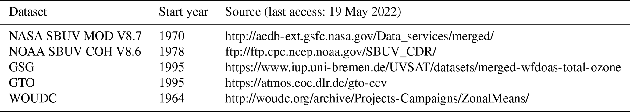
We report on updated trends using different merged zonal mean total ozone datasets from satellite and ground-based observations for the period from 1979 to 2020. This work is an update of the trends reported in Weber et al. (2018) using the same datasets up to 2016. Merged datasets used in this study include NASA MOD v8.7 and NOAA Cohesive Data (COH) v8.6, both based on data from the series of Solar Backscatter Ultraviolet (SBUV), SBUV-2, and Ozone Mapping and Profiler Suite (OMPS) satellite instruments (1978–present), as well as the Global Ozone Monitoring Experiment (GOME)-type Total Ozone – Essential Climate Variable (GTO-ECV) and GOME-SCIAMACHY-GOME-2 (GSG) merged datasets (both 1995–present), mainly comprising satellite data from GOME, SCIAMACHY, OMI, GOME-2A, GOME-2B, and TROPOMI. The fifth dataset consists of the annual mean zonal mean data from ground-based measurements collected at the World Ozone and Ultraviolet Radiation Data Centre (WOUDC).
Trends were determined by applying a multiple linear regression (MLR) to annual mean zonal mean data. The addition of 4 more years consolidated the fact that total ozone is indeed slowly recovering in both hemispheres as a result of phasing out ozone-depleting substances (ODSs) as mandated by the Montreal Protocol. The near-global (60∘ S–60∘ N) ODS-related ozone trend of the median of all datasets after 1995 was 0.4 ± 0.2 (2σ) %/decade, which is roughly a third of the decreasing rate of 1.5 ± 0.6 %/decade from 1978 until 1995. The ratio of decline and increase is nearly identical to that of the EESC (equivalent effective stratospheric chlorine or stratospheric halogen) change rates before and after 1995, confirming the success of the Montreal Protocol. The observed total ozone time series are also in very good agreement with the median of 17 chemistry climate models from CCMI-1 (Chemistry-Climate Model Initiative Phase 1) with current ODS and GHG (greenhouse gas) scenarios (REF-C2 scenario).
The positive ODS-related trends in the Northern Hemisphere (NH) after 1995 are only obtained with a sufficient number of terms in the MLR accounting properly for dynamical ozone changes (Brewer–Dobson circulation, Arctic Oscillation (AO), and Antarctic Oscillation (AAO)). A standard MLR (limited to solar, Quasi-Biennial Oscillation (QBO), volcanic, and El Niño–Southern Oscillation (ENSO)) leads to zero trends, showing that the small positive ODS-related trends have been balanced by negative trend contributions from atmospheric dynamics, resulting in nearly constant total ozone levels since 2000.
- Article
(2784 KB) - Full-text XML
-
Supplement
(380 KB) - BibTeX
- EndNote


The stratospheric ozone layer protects the biosphere from harmful UV radiation. How much UV reaches the surface depends, among other factors like clouds, on the overhead total ozone column. The discovery of the Antarctic ozone hole (Chubachi, 1984; Farman et al., 1985; Solomon et al., 1986) raised awareness of the need to protect the ozone layer that culminated in the 1985 Vienna Convention and a commitment to take actions. One of the actions was the signing of the Montreal Protocol in 1987 that started the phaseout of ozone-depleting substances (ODSs), which are sufficiently long-lived to reach the stratosphere and release active halogens that destroy ozone (e.g. Solomon, 1999). As a consequence of the Montreal Protocol and its later amendments, stratospheric halogens started to decline in the middle 1990s (e.g. Anderson et al., 2000; Solomon et al., 2006). A corresponding ozone increase has been detected from satellite and ground-based observations, particularly in the upper stratosphere (Braesicke et al., 2018, and references therein).
Changes in total ozone column are representative of lower stratospheric ozone changes as the majority of ozone resides in the lower stratosphere (“ozone layer”). Lower stratospheric ozone is sufficiently long-lived to be influenced by transport and circulation changes. The rapid increase in Northern Hemisphere total ozone in the late 1990s (Harris et al., 2008) revealed the important role of ozone transport via the Brewer–Dobson (BD) circulation. These circulation changes also cause large variability on inter- and intra-annual timescales in lower stratospheric ozone and the total column (e.g. Fusco and Salby, 1999; Randel et al., 2002; Dhomse et al., 2006; Harris et al., 2008; Weber et al., 2011) and make detection of ozone recovery challenging. Apart from the observed variability, zonal mean total ozone levels in both hemispheres remained stable since about the year 2000 (e.g. Weber et al., 2018). The success of the Montreal Protocol is nevertheless undisputed as the earlier decline in total ozone was successfully stopped (Mäder et al., 2010; Braesicke et al., 2018).
Global and continuous ozone observations from satellites through 2020 now span a total time period of 42 years, of which 25 years cover the period after the stratospheric halogen peak (around 1995). The added years should help in improving the statistical significance of ozone recovery after the middle 1990s (Weatherhead et al., 2000). This paper reports on updated zonal mean total ozone trends from Weber et al. (2018) (abbreviated to W18 in the following) by adding 4 more years of data (2017–2020) to five merged total ozone datasets. In our earlier study, ozone recovery trends in the extratropics were on the order of +0.5 %/decade. The derived trends depend on the proper treatment of dynamical processes in the multilinear regression. Changes in circulation and ozone transport, in part due to increasing greenhouse gas (GHG) levels, have variability on decadal and longer timescales and can therefore mask ODS-related recovery trends. Longer data records are helpful to further disentangle the various processes responsible for long-term changes in ozone. In this work we focus specifically on trend estimates directly related to ODS changes in order to evaluate the direct impact from the Montreal Protocol.
The main results from our earlier paper (W18) were latitude-dependent annual mean total ozone trends from the middle 1990s to 2016, which were reported to be on average +0.5 %/decade in the extratropics and only significant in the Southern Hemisphere (SH; W18). Since W18 was published, there have been three recent studies on global and regional ozone column trends (Bozhkova et al., 2019; Krzyścin and Baranowski, 2019; Coldewey-Egbers et al., 2022). Krzyścin and Baranowski (2019) derived total ozone column trends from a multivariate linear regression (MLR) applied to the Multi-Sensor Reanalysis-2 (MSR-2) total ozone dataset up to 2017 (van der A et al., 2015). In their MLR, they split the entire period from 1978 to 2017 into three periods with separate trends (either independent or piecewise linear). The choice of two inflection points was chosen from fits having minimum fit root mean square (rms) errors. As stratospheric halogens have been declining steadily since the middle 1990s, the interpretation of the segmented trends is difficult. Trends of the first period (before middle 1990s) are in agreement with W18 and this study.
Bozhkova et al. (2019) applied a regression to TOMS and OMI total ozone at northern hemispheric mid-latitudes using the approach by Bloomer et al. (2010), first applied to surface ozone and temperature data at selected stations in the United States. Without using any proxy data, the regression estimates trends of the seasonality expressed as Fourier series. Attribution of physical and chemical processes to the long-term changes is therefore not possible, as also stated by the authors. Latitude- and longitude-dependent total ozone trends are reported by Coldewey-Egbers et al. (2022) derived from the ESA/DLR GTO-ECV dataset, which is one of the five observational datasets used in this study. They report significant positive linear trends after 1995 over large regions in the extratropical Southern Hemisphere (SH), while in the tropics and Northern Hemisphere (NH) they are mostly insignificant. Consequently, they only reported significant zonal mean positive trends in the SH.
In Sect. 2 the updates in the five merged datasets are briefly discussed. In Sect. 3 the multiple linear regression (MLR) as used in our trend analysis is described and discussed. Section 4 presents the total ozone trend results in broad zonal bands: near-global, southern and northern hemispheric extratropics, and tropics. In Sect. 5, latitude-dependent annual mean total ozone trends are presented and discussed. Polar ozone trends for the months where polar ozone losses are largest (e.g. during ozone hole season) are presented in Sect. 6. In Sect. 7, a summary and final remarks are given.
Five merged total ozone datasets are used in this study of which one dataset is based upon ground-based observations. All others are based on satellite observations. Two different merged datasets are derived from the series of SBUV and SBUV-2 satellite instruments (SBUV MOD V8.7 from NASA and SBUV COH V8.6 from NOAA), operating continuously since the late 1970s. The other two merged datasets are based largely upon the series of European satellite spectrometers GOME, SCIAMACHY, GOME-2A, and GOME-2B, with different retrieval and merging algorithms applied (University of Bremen GSG and ESA/DLR GTO-ECV datasets). These datasets start in 1995.
The ground-based dataset is the monthly mean zonal mean data from the network of Brewers, Dobsons, SAOZ (Système d'Analyse par Observations Zénithales), and filter instruments collected at the World Ozone and Ultraviolet Radiation Data Centre (WOUDC) (Fioletov et al., 2002). In addition, a brief description of the model data from the CCMI Phase 1 is given. The sources of observational data are listed in Table 1, and brief descriptions of the datasets are given in the following. Annual mean time series of all five merged datasets are in very good agreement with each other to within a few Dobson units (DU; see also Fig. 2.58 in Weber et al., 2021). All datasets cover the entire earth, except for months and latitudes under polar night conditions.
2.1 NASA SBUV MOD V8.7
The NASA Merged Ozone Data (MOD) time series is constructed using data from the Nimbus 4 BUV, Nimbus 7 SBUV, and six NOAA SBUV-2 instruments numbered 11, 14, and 16–19, and the Ozone Mapping and Profiler Suite Nadir Profiler (OMPS-NP) instrument aboard the Suomi-NPP satellite (Frith et al., 2014, 2022).The instruments are of similar design, and measurements from each are processed using the same V8.7 algorithm. To maintain consistency over the entire time series, the individual instrument records are analysed with respect to each other, and absolute calibration adjustments are applied as needed based on comparison of radiance measurements during periods of instrument overlap (DeLand et al., 2012).
Version 8.7 uses the same core algorithm as Version 8.6 (Bhartia et al., 2013) but includes new inter-instrument calibration adjustments for instrument records since 2000 (NOAA-16 SBUV/2 through OMPS NP) based on a new approach to radiance intercomparisons across overlapping instruments (Kramarova et al., 2022). Version 8.7 also incorporates an updated a priori ozone profile climatology with improved tropospheric representation based on GMI model output and diurnal adjustments to ensure the a priori profile correctly reflects the local solar time of each measurement (Ziemke et al., 2021). A post-retrieval diurnal correction is applied to adjust each instrument record to an equivalent measurement time of 13:30 (Frith et al., 2020). Remaining offsets between instruments exist (mostly below 5 % for layers, below 1 % for total ozone), but their cause is not understood. We therefore do not make adjustments to the data. Rather we set limitations on the data included in the merged product based on data quality analysis by the instrument team and on comparisons with independent measurements (DeLand et al., 2012; Kramarova et al., 2013, 2022). For merging, data are averaged during periods with multiple operational instruments. The Version 8.7 MOD data contain monthly zonal mean ozone profiles in mixing ratio on pressure levels and in Dobson units on layers. The total ozone is then provided as the sum of the layer data.
2.2 NOAA SBUV COH V8.6
The NOAA COH (cohesive) dataset is a simple extension in time of the dataset appearing in W18. The data include v8.6 SBUV on Nimbus 7, v8.6 SBUV/2 from NOAA 9, 11, 16 to 19, and v3r2 OMPS Nadir Profiler (NP) on Suomi-NPP as available from NESDIS STAR. The merging approach differs from NASA MOD in two important ways. NASA MOD averages data from all relevant satellites in any time period for which the data meet certain quality criteria. NOAA COH uses data from a single “best” satellite in any time period. Which satellite is used depends on known data quality issues, on minimizing the solar zenith angle of the measurement, and on maximizing global coverage. NOAA COH does not shift to an equivalent measurement time (13:30) but performs an adjustment between data from differing satellites. For post-2000 data, where drift of the measurement time is minimized, the data are all adjusted to NOAA 18. For data from 1999 and prior to this year, the inter-satellite overlap is often short, and the satellite drift often significant; we choose only to adjust NOAA 9 to the two branches NOAA 11 prior to and after the NOAA 9 time period. The total ozone is calculated from the sum of the adjusted profile layer data. By vertical integration, many of the layer adjustments to a large extent cancel out such that the final total ozone product is altered by less than 1 %, and in most cases by less than 0.5 %, from the original satellite datasets.
2.3 University of Bremen GSG
The merged GOME, SCIAMACHY, GOME-2A, and GOME-2B (GSG) total ozone time series (Kiesewetter et al., 2010; Weber et al., 2011, 2018) consists of total ozone data that were retrieved using the University of Bremen weighting function DOAS (WFDOAS) algorithm (Coldewey-Egbers et al., 2005; Weber et al., 2005; Orfanoz-Cheuquelaf et al., 2021). The merging of the data has been described in W18. The most recent modification was to replace GOME-2A data after January 2015 with data from GOME-2B (2012–present), which has a better global coverage after changes in the GOME-2A scanning pattern. Latitude-dependent bias corrections for GOME-2B were applied from the overlapping period 2014–2020 with GOME-2A.
2.4 DLR/ESA GTO-ECV
The latest version of the GOME-type Total Ozone Essential Climate Variable (GTO-ECV) data record (Coldewey-Egbers et al., 2015, 2022; Garane et al., 2018) has been generated as part of the European Space Agency’s Climate Change Initiative+ ozone (ESA_CCI+ ozone) project. Total columns from six sensors (GOME, SCIAMACHY, OMI, GOME-2A, GOME-2B, and TROPOMI), retrieved with the GOME Direct Fitting (GODFIT) version 4 algorithm (Lerot et al., 2014; Garane et al., 2018), were combined into a coherent record that covers the period 1995–2020. OMI was used as a reference instrument, and the other sensors were adjusted by means of latitude- and time-dependent correction factors determined from overlap periods.
2.5 WOUDC data
The WOUDC zonal mean dataset (Fioletov et al., 2002) was formed from ground-based measurements by Dobson, Brewer, SAOZ instruments, and filter ozonometers available from the WOUDC. The overall performance of the ground-based network was discussed by Fioletov et al. (2008), and the present state of the network is described by Garane et al. (2019). This dataset is provided by the WOUDC and updated regularly.
First, ground-based measurements were compared with an ozone “climatology” (monthly means for each point of the globe) estimated from satellite data for 1978–1989. Then, for each station and for each month, the deviations from the climatology were calculated, and a zonal mean value for a particular month was estimated as a mean of these deviations. The calculations were done for 5∘ wide zonal bands. In order to take into account various densities of the network across regions, the deviations of the stations were first averaged over 5 by 30∘ cells, and then the zonal mean was calculated by averaging these first set of averages over the 5∘ wide zonal band. Then the zonal averages were smoothed by approximating them using Legendre polynomials.
The WOUDC dataset was compared with merged satellite time series and demonstrated a good agreement (Chiou et al., 2014). Estimates based on relatively sparse ground-based measurements, particularly in the tropics and Southern Hemisphere, may not always reproduce monthly zonal mean fluctuations well. However, seasonal (and longer) averages can be estimated with a precision comparable with satellite-based datasets (∼1 %) (Chiou et al., 2014).
2.6 Chemistry–climate model data
In this study, output from the chemistry–climate models (CCMs) and chemistry-transport models (CTMs) participating in phase 1 of CCMI (Chemistry-Climate Model Initiative) is used (Eyring et al., 2013). An overview of the models, together with details particular to each model and an overview of the available simulations, is given in Morgenstern et al. (2017), along with a detailed description of the full forcings used in the reference simulations (Eyring et al., 2013; Hegglin et al., 2016). Here we have used median total column ozone from 17 models taking part in the REF-C2 experiment, an internally consistent seamless simulation between 1960 and 2100.
2.7 Data preparation
From the zonal mean monthly mean data in 5∘ latitude steps (all datasets), annual means were calculated. Wider zonal bands (like 35–60∘ N) were averaged from the 5∘ data using area weights (see W18). All annual mean zonal mean time series were bias-corrected by subtracting the difference to the mean of all datasets during the 1998–2008 period. The multi-dataset mean was then added back to each dataset, such that all bias-corrected time series are provided in units of the total column amounts (W18). However, the trend results derived from them are identical to those derived using anomaly time series.
Like in our earlier study, the GSG and GTO-ECV time series were extended from 1995 back to 1979 using the bias-corrected NOAA data. This way one ensures that all terms other than the trend terms are determined from the full time (1979–2020) period. The NOAA data were preferred here over the NASA data, as the former have shorter data gaps after the major volcanic eruption from Mt. Pinatubo in 1991 and subsequent years.
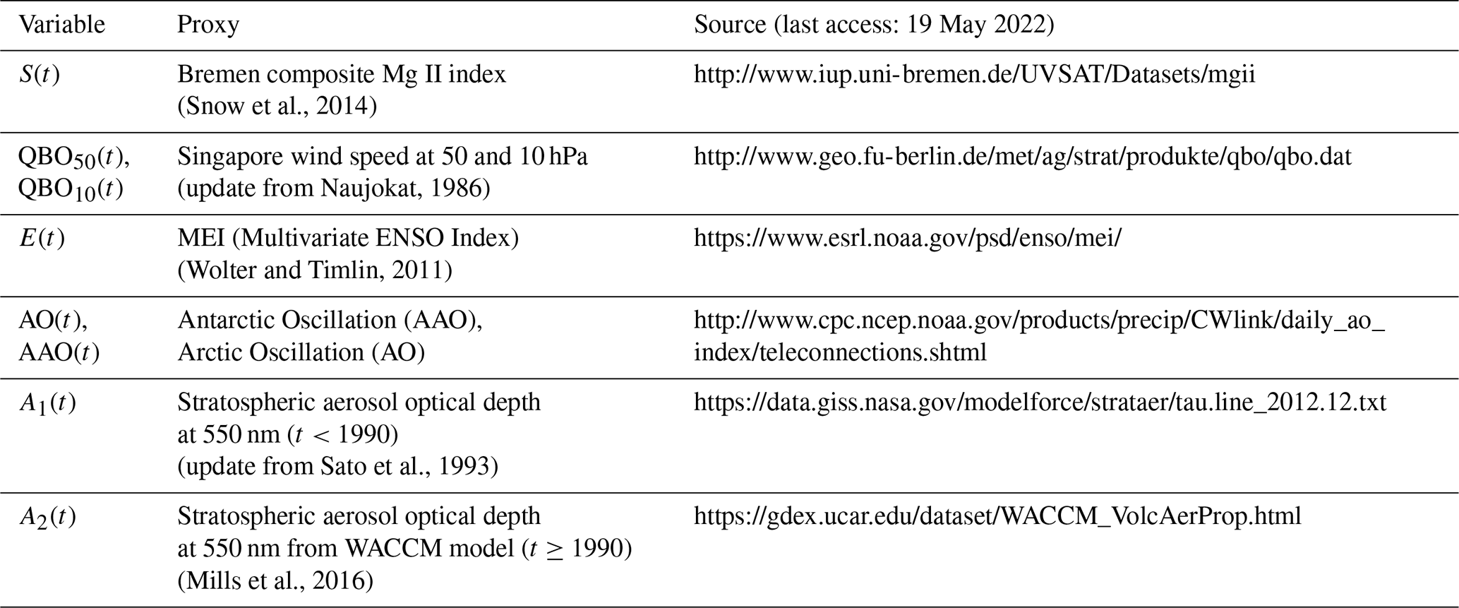
The standard MLR model is identical to the one used in W18 and includes two independent linear trend terms (before and after the ODS-related turnaround year t0=1995), two aerosol terms (Mt. Pinatubo 1992 and El Chichón 1983), a solar cycle term, two Quasi-Biennial Oscillation (QBO) terms (50 and 10 hPa), and ENSO (El Niño–Southern Oscillation):
y(t) is the annual mean zonal mean total ozone time series and t the year of observations. The coefficients b1 and b2 are the linear trends before and after t0. In order to make both trends independent of each other (or disjoint), two y intercepts (a1 and a2) are added. The multiplication of the independent variable t with Xi(t) in the first four terms of Eq. (1) describes mathematically that the first two terms only apply to the period before and the third and fourth terms to the period after the turnaround year. X1(t) and X2(t) are given by
and
respectively. The independent trends before and after t0 are favoured over the use of piecewise linear trends or the use of EESC as a proxy time series (see detailed discussions in W18). The maximum of the effective equivalent stratospheric chlorine (EESC) was reached at about the year t0=1995 (Newman et al., 2007), except for the polar region () where t0=2000 (Newman et al., 2006, 2007).The contributions from the QBO, 11-year solar cycle, and stratospheric aerosols are standard in total ozone MLR analyses (e.g. Staehelin et al., 2001; Reinsel et al., 2005). ϵ(t) is the residual from fitting the coefficients to match the regression model (right side) to the observations. By using annual mean total ozone, auto-correlation is very low here (below 0.1 in absolute value for a shift by 1 year) so that no further additional auto-regression term as commonly used for monthly mean ozone time series is needed (e.g. Dhomse et al., 2006; Vyushin et al., 2007).
The stratospheric aerosols are dominated by the major volcanic eruptions from El Chichón (1982) and Mt. Pinatubo (1991). Enhanced aerosols in the lower stratosphere lasting for a few years impact both ozone chemistry and transport (Schnadt Poberaj et al., 2011; Dhomse et al., 2015). The stratospheric aerosol optical depth (SAOD) at 550 nm from Sato et al. (1993) is used as the explanatory variable before 1990 (includes the El Chichón event), while newer data from the WACCM model (Mills et al., 2016) are used for the period after 1990 (include Mt. Pinatubo major volcanic eruption and the series of more minor volcanic eruptions from the last decade). Missing years after 2015 were filled with background values from the late 1990s.
As mentioned in W18, there is not a sufficient number of months and/or 5∘ latitude bands available in the SBUV data records for some years, and for these years annual means were treated as missing data. Annual means were only used in the regression if at least 80 % of the 5∘ bands of the data were contained in the broad zonal bands and 80 % of months available in that year. If annual means of the years 1982 and 1983 are missing, the “El Chichon” term is not used in the MLR; similarly if missing all years from 1991 to 1994, the “Pinatubo” term is excluded in the MLR.
The MLR equation, Eq. (1), without the P(t) term has been commonly applied for determining trends from ozone profile data (e.g. Bourassa et al., 2014, 2018; Harris et al., 2015; Tummon et al., 2015; Sofieva et al., 2017; Steinbrecht et al., 2017). The extra term P(t) in Eq. (1) accounts for additional factors of dynamical variability that have been used in different combinations and definitions (e.g. accumulated, time-lagged) in the past. It includes contributions from the Arctic (AO) and Antarctic Oscillation (AAO), and the Brewer–Dobson circulation (BDC) (e.g. Reinsel et al., 2005; Mäder et al., 2007; Chehade et al., 2014; Weber et al., 2018). The BDC terms are usually described by the eddy heat flux at 100 hPa that is considered a main driver of the BDC (Fusco and Salby, 1999; Randel et al., 2002; Weber et al., 2011). The term P(t) is given as follows:
In W18 the AAO term was not included. Table 2 summarizes the sources of the proxy data used here. The BDCn and BDCs are 100 hPa eddy fluxes in the Northern (n) and Southern Hemisphere (s). The calculation of the BDC proxy from the monthly mean eddy heat fluxes is described in detail in W18. In this study, the eddy heat flux data were derived from the ERA-5 reanalysis (Hersbach et al., 2020).
(Snow et al., 2014)(update from Naujokat, 1986)(Wolter and Timlin, 2011)(update from Sato et al., 1993)(Mills et al., 2016)Table 2Sources of explanatory variables/proxy time series used in the MLR.
One may argue that the addition of P(t) will lead to some overfitting by the MLR. We justify this addition as it enables us to obtain MLR fits matching the extreme events like very high annual mean ozone in the NH in 2010 and the very large warming events above Antarctica in 2002 and 2019 with unusually high ozone. The better the dynamical variations are represented in the MLR, the more likely we can separate out dynamical trend contributions and the linear trend terms best approximate EESC-related trends. In our previous study, only selected terms from P(t) were used dependent on their significance in specific zonal bands. Retaining all terms in all MLRs leads to smoother behaviour in the latitude-dependent ozone response.
The various proxy time series, in particular the atmospheric-dynamics-related ones, are partially correlated. One way to improve upon this is to orthogonalize them. Doing so will not change the MLR fit results, but some contributions from the original proxy terms will be redistributed among the proxies that were orthogonalized. It is also common to detrend the proxy time series. In that case, all linear changes of the various processes or proxies will be added up in the linear trend term which makes attribution impossible. For these reasons, we do not detrend nor orthogonalize the proxy time series in this study. Our goal here is that linear changes of all the processes as expressed by the various proxy terms shall be excluded from the linear trend terms such that the linear trends can be attributed as close as possible to ODS changes.
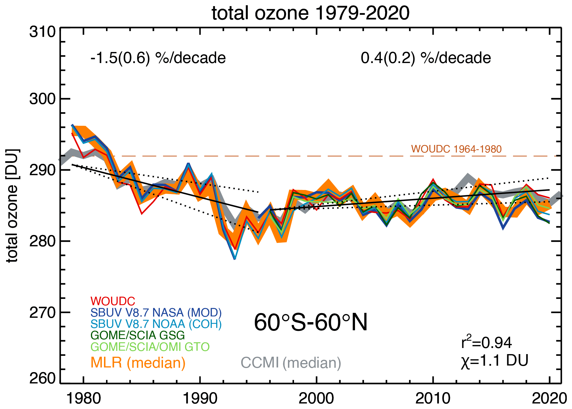
Figure 1Near-global (60∘ S–60∘ N) total ozone time series of five bias-corrected merged datasets. The thick orange line is the result from applying the full MLR (Eqs. 1 and 4) to the median time series. The square of the correlation between observations and MLR is given by r2. χ2 is the sum square of the differences between median observational and MLR time series divided by the degrees of freedom (difference between the number of years, n, and number of parameters used in the MLR, m). The solid lines indicate the linear trends before and after the ODS peak, respectively. The dotted lines indicate the 2σ uncertainty of the MLR trend estimates. Trend numbers are indicated for the pre- and post-ODS peak period in the top part of the plot. Numbers in parentheses are the 2σ trend uncertainty. The dashed orange line shows the mean ozone level from 1964 until 1980 from the WOUDC data. The thick grey line is the median of 17 chemistry–climate models from the CCMI.

Figure 2Same as Fig. 1 but for broad zonal bands: (a) 35–60∘ N (Northern Hemisphere), (b) 20∘ S–20∘ N (tropics), and (c) 35–60∘ S (Southern Hemisphere).
Figure 1 shows the near-global mean time series (60∘ S–60∘ N) of the five bias-corrected merged datasets. The thick orange line is the MLR time series from applying the full regression model (Eqs. 1 and 4) to the median of the five time series. A total of 94 % of the variability in total ozone is well captured by the full MLR. A positive trend of (2σ) %/decade after 1995 is derived. This trend is about one-third of the absolute trend during the phase of increasing ODSs before 1995, which is %/decade. The ratio of trends before and after 1995 is very close to the ratio of rate changes in the effective equivalent stratospheric chlorine (EESC) before and after the middle 1990s (Dhomse et al., 2006; Newman et al., 2007). Therefore, the observed linear trend of roughly half a percent per decade up to 2020 can be attributed to reductions in ODSs following the Montreal Protocol. This ODS-related recovery appears statistically robust (to within 2σ), even though the ozone levels have stayed more or less constant apart from the year-to-year variability since the year 2000. The magnitude of the post-ODS peak trend remained unchanged from W18. The trend results vary only slightly if the turnaround year (1995) of the ODS change is shifted by 1 year back and forward. Even if the MLR fit of the post-ODS peak period is limited to years after 2000, the ODS-related trend remains robust at +0.5(0.3) %/decade.
The current near-global ozone level (2017–2020) is about 2.3 % below the average from the 1964–1980 time period, the latter derived from the WOUDC data (see Fig. 1). Recovery of total ozone to the 1980 level is generally not expected before about the middle of this century (Braesicke et al., 2018). The near-global total ozone time series from the median of the 17 CCMI chemistry–climate models is in very good agreement with the observations from which we conclude that the chemical and dynamical changes in total ozone under current ODS and greenhouse gas (GHG) scenarios are well understood and consistent with observations.
Figure 2 shows the ozone time series in the Northern (NH) and Southern Hemisphere (SH) as well as in the tropics. Again, the current ozone levels are well below the 1964–1980 mean, specifically −3.6 % and −4.7 % in the NH and SH (35–60∘ latitudes), respectively. The lower value in the SH is due to the influence from the spring Antarctic ozone hole, which exhibits the largest local ozone depletion and leads to mixing of ozone-depleted air in the middle latitudes (Atkinson et al., 1989; Millard et al., 2002). ODS-related trends are +0.5(0.5) and +0.7(0.6) %/decade in the NH and SH, respectively. Within the trend uncertainty, the 1 : 3 ratio in the linear trends before and after the ODS peak in 1995 is close to the ratio of the rate change in the EESC in both hemispheres.
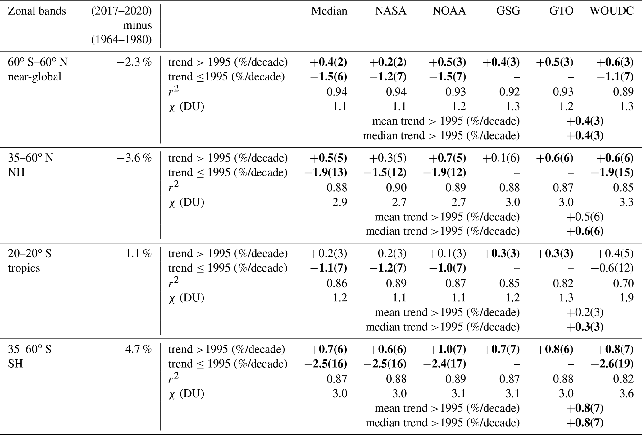
In the tropics the linear trend after 1995 is close to zero and insignificant (Fig. 2 and Coldewey-Egbers et al., 2022). Table 3 summarizes the MLR results in the broad zonal bands from the individual datasets and the median time series as well as the mean and median of the individual trends.
In most cases the results from the individual datasets are highly consistent, in particular for the near-global time series. All datasets indicate significant near-global ODS-related trends of around half a percent per decade. The trend derived from the NASA data is a bit lower at +0.2 %/decade. The median and mean trends of all datasets agree here with the trends of the median time series as shown in Figs. 1 and 2. For the narrower zonal bands, not all datasets show significant trends after 1995. The NASA and GSG datasets show lower trends in the NH (+0.3 and +0.1 %/decade, respectively), while all others are between +0.5 and +0.7 %/decade and significant. In the SH, all trends agree to within 0.001 %/decade (+0.7 %/decade), except for the NOAA dataset showing a somewhat higher trend of +1 %/decade.
Table 31979–1995 and 1996–2020 annual mean total ozone trends in various broad zonal bands. Uncertainties are given as 2σ; trends in bold have an absolute magnitude equal to or larger than 2σ. r2 is the square Pearson correlation between time series of observations and MLR and χ the residual defined as , where obsi denotes the observations, modi the MLR model, n the number of data (years) in the time series, and m the number of parameters fitted. All results are obtained using the full MLR. The second column shows the percent difference of the current total ozone level (2017–2020) with respect to the period before 1980 derived from the median time series.
Bold numbers: statistical significance at 2σ.
In the tropics, trends are close to zero, with the exception of the GSG and GTO datasets that have very small and barely significant positive trends of +0.3 ± 0.3 %/decade. The variations in the trend results from the different datasets are most likely due to some residual drifts in the datasets that are not accounted for in the data merging. With the use of the full MLR with all terms and with 4 years added in the time series, the ozone trends in the various zonal bands after 1995 remain quite similar to the results reported in W18, but uncertainties are slightly reduced.
Table 4 shows different MLR settings applied to the median total ozone time series in broad zonal bands (as defined in Table 3). Here the results from the standard and full MLR are listed. In addition, we applied an iterative MLR approach where statistically insignificant terms (2σ criterion) from Eq. (4) and the El Niño term are successively excluded before the final MLR run. The inclusion of the dynamical proxies generally improved the MLR fit (r2 and χ values). Except for the NH zonal band (35–60∘ N), the various MLR settings yield nearly the same post-ODS peak trends for all broad zonal bands (Table 4). There are, however, larger changes in the trends before the middle 1990s. In the extratropics the early-period trends are lower in the standard retrieval (−4.0 % versus −1.9 %/decade in the NH and −3.1 % versus −1.9 %/decade in the SH). This means that atmospheric dynamics and transport changes contributed to lower early-period extratropical total ozone trends in the standard regression (due to the lack of these dynamical terms in the MLR). The opposite is the case in the tropics, where the early-period trends in the standard MLR are slightly higher than in the full MLR. This opposite behaviour is consistent with ozone transport patterns due to the Brewer–Dobson circulation.
It appears that the post-ODS trends are in most cases unchanged, regardless of the number of extra terms used in the MLR. The linear trend term is the only low-frequency term in the MLR equations, while the dynamical proxies have some high-frequency contributions. This makes the trend estimates rather robust and less sensitive to the various other terms used in the MLR. The only significant changes in the post-ODS peak trends are seen in the NH extratropics. In the standard MLR this trend is zero, while the full and iterative MLR shows trends of half a percent per decade. The sum of the ODS-related trend (full MLR) and atmospheric dynamics contribution (difference in the trends between full and standard MLR) cancel out to result in a zero trend in the standard MLR. The negative dynamical trend contribution in the NH is further discussed later in the paper. The correlation between regression and observations is substantially lower in the standard retrieval (r2=0.74 versus 0.88), which indicates that the standard MLR seems not to capture all variability and changes of total ozone.
In order to document the changes from the current MLR fits (Table 4) to results from the period up to and including 2016 (as in W18), the different MLR settings were applied to the current data for the shorter period as summarized in Table S1 (see Supplement). Note that the results in Table S1 may differ from W18 as the merged datasets have been updated, and data before 2017 may have changed as well. Results from the shorter time period are nearly identical to those shown in Table 3. There is one notable change. The uncertainties of the NH trends from the full MLR up to 2020 are reduced such that these trends have become barely significant (2σ). The NH post-ODS peak trend of the standard MLR is slightly positive up to 2016 but statistically insignificant and within the uncertainties not different from the current results.
Table 4Different MLR settings applied to the broad zonal mean median ozone time series. For explanations of terms, see Table 3. Standard MLR is based upon Eq. (1) with P(t)=0. Iterative MLR means that only terms of P(t) and El Niño term are fitted when they are statistically significant (2σ), while full MLR includes all terms in Eq. (1) and P(t).
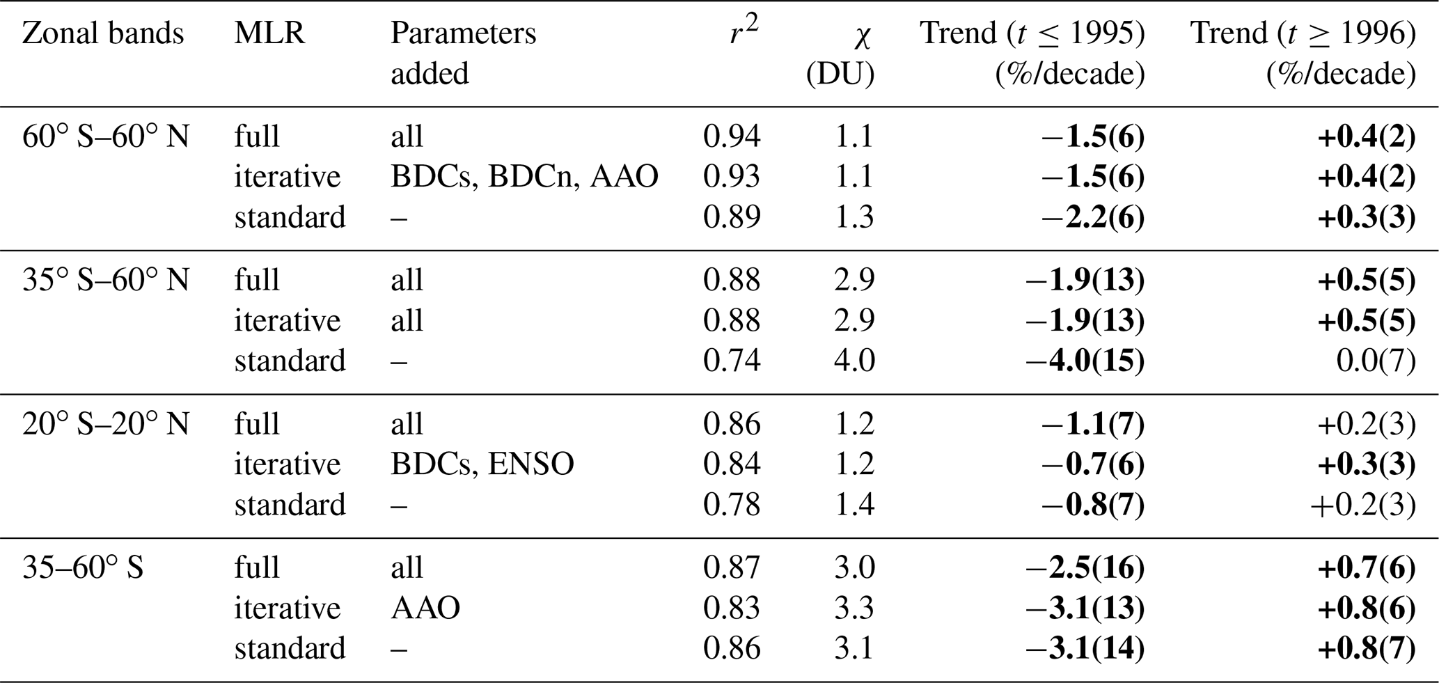
bold numbers: statistical significance at 2σ.
Latitude-dependent trends in steps of 5∘ are shown from 60∘ S to 60∘ N for all five merged datasets (thin lines) in Fig. 3. The two thick blue and red lines are the results before and after 1995 from applying the full MLR to the median time series, including 2σ uncertainties shown as error bars. In the extratropics, the ODS-related trends are on the order of +0.5 %/decade, with 2σ uncertainties of about the same magnitude. In the SH, the trends continuously increase to nearly +1.3 %/decade in the 55–60∘ S band, while in the NH, the trends remain unchanged up to the highest latitudes shown. In the tropics, trends are close to zero. One notable change from W18 is that the tropical trends during the ODS rising phase are now more negative (down to −1 %/decade), while before they were mainly close to zero. This may be caused by the additional proxy terms used in this study.
After 1995, all trends of all datasets are in good agreement to within ±0.3 %/decade. There are some notable differences in the northern subtropical and northern tropical trends for the WOUDC data (up to +1 %/decade) compared to the other datasets, which is most likely caused by larger uncertainties due to the sparsity of ground-based data at these latitudes. The trend uncertainties are generally larger for the early period before 1996, which is caused by the different lengths of the periods before (17 years) and after 1995 (25 years).
The dashed pink line shows the expected ODS-related trends when applying the 1 : 3 ratio (corresponding to the rate change of the EESC) to the trends before 1996. It agrees quite well in the extratropics with the independent linear trend estimates and therefore give us confidence that ozone is responding to the long-term ODS decline. The expected tropical ODS-related trends are slightly positive, while the MLR regressions rather suggest near-zero trends, but they still agree within their uncertainties. In the NH extratropics, the expected ODS-related trend is slightly higher than the observed trends but also agrees within the uncertainties of the observed trends.
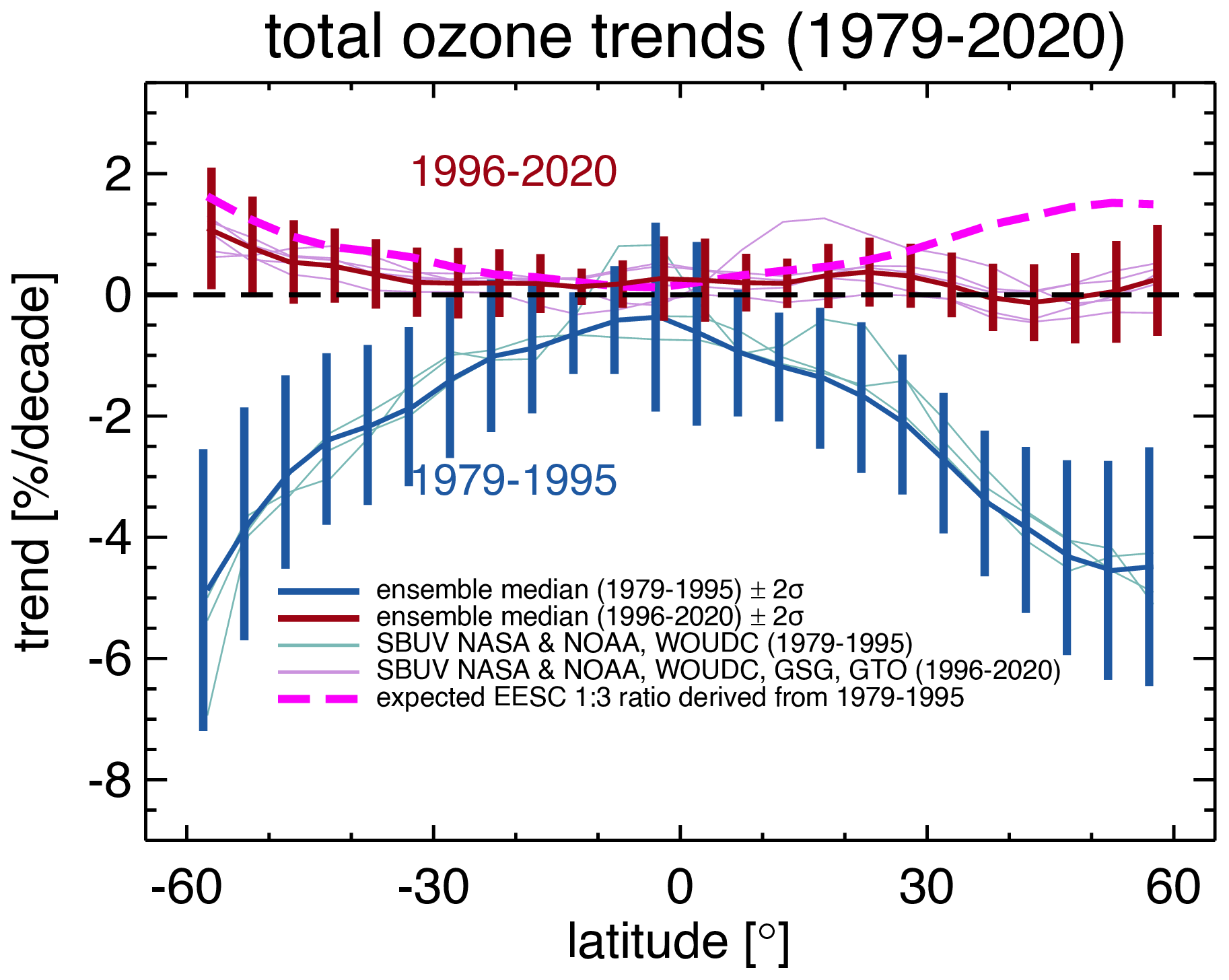
In order to elucidate the interpretation of the independent linear trends after 1995, we repeated the analyses using the standard MLR, which excludes several terms responsible for changes in atmospheric dynamics and transport (Eq. 1 with P(t)=0). The latitude-dependent trends from the standard MLR are shown in Fig. 4. While the observed trends for both MLRs are nearly unchanged in the SH, the NH trends are reduced to zero in the NH extratropics. On the other hand the tropical trends before 1996 are closer to zero. The expected ODS-related trends (from the 1 : 3 EESC ratio) have become larger, with increases to +1.5 %/decade at the higher latitudes now in both hemispheres. The most obvious result is that the independent linear trends after 1995 in the NH being close to zero now clearly deviate from the expected 1 : 3 ratio. It appears that the additional atmospheric dynamics terms in the regression balance the positive trends from the full MLR, which explains why total ozone in the NH has appeared more or less stable during the last 2 decades (Fig. 2a).
The declining trends in the NH before 1996 (Fig. 4a) are stronger in the standard MLR and are comparable to the SH (about −4 %/decade near 60∘ latitude). On the other hand, ODS-related trends are expected to be somewhat stronger in the SH as the influence from polar ozone losses on mid-latitude ozone is thought to be larger in the SH, since Arctic ozone losses are more sporadic and generally smaller. In that regard, the trends from the full MLR seem to support this notion.
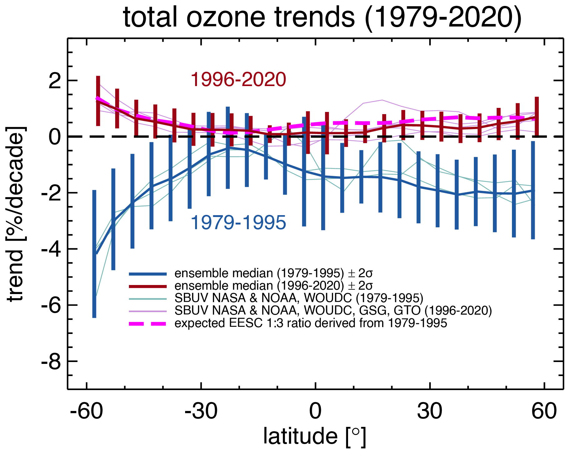
Figure 3Latitude-dependent ozone trends in steps of 5∘ from applying the full MLR (Eqs. 1 and 4) to the median time series of the five merged total ozone datasets. Trends and 2σ standard deviations are shown in blue for the time period before 1995 and in red after 1995. The thin lines show the trends of the individual total ozone datasets. The dashed pink lines are the post-ODS peak trends as expected from the 1 : 3 ratio (corresponding to changes in the stratospheric halogen), applied to the median time series' trends before 1996.
The comparisons of trends from the standard and full MLR reveal that the NH ODS-related ozone recovery is balanced by long-term changes in atmospheric dynamics (circulation and transport changes), or in other words the near-zero linear post-ODS peak trends are caused by the combination of ODS-related recovery and dynamical changes. These two signals are more clearly separated in the full MLR. Before discussing this further, we will take a look at the contributing factors or terms in the MLR. Figure 5 shows the maximum response of the various terms in Eqs. (1) and (4) as a function of latitude (from the fit to the median time series).
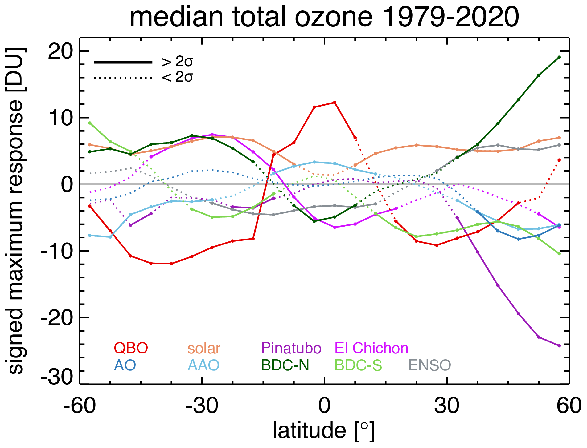
Figure 5Signed maximum time series contribution from various terms in the full MLR equation applied to the median of the five merged total ozone datasets. Solid line indicates values of fit coefficients that are larger than their 2σ uncertainty. The sign of the BDCs proxy time series is reversed, so that in both hemispheres positive BDC term values correspond to enhanced Brewer–Dobson circulation. Negative values correspond to an anti-correlation of the ozone response to the proxy. For instance, positive solar contributions mean high solar activity, which leads to more ozone.
Well-known factors like solar activity and QBO show the expected behaviour, i.e. more ozone during solar maximum at all latitudes (see, for example, W18) and the opposite sign in the QBO response between inner tropics and extratropics (Bowman, 1989; Baldwin et al., 2001). The solar response is of similar magnitude at all latitudes, which means that the solar effect in the lower stratosphere is mostly indirect via changes in temperature and associated atmospheric circulation changes (e.g. Dhomse et al., 2022).
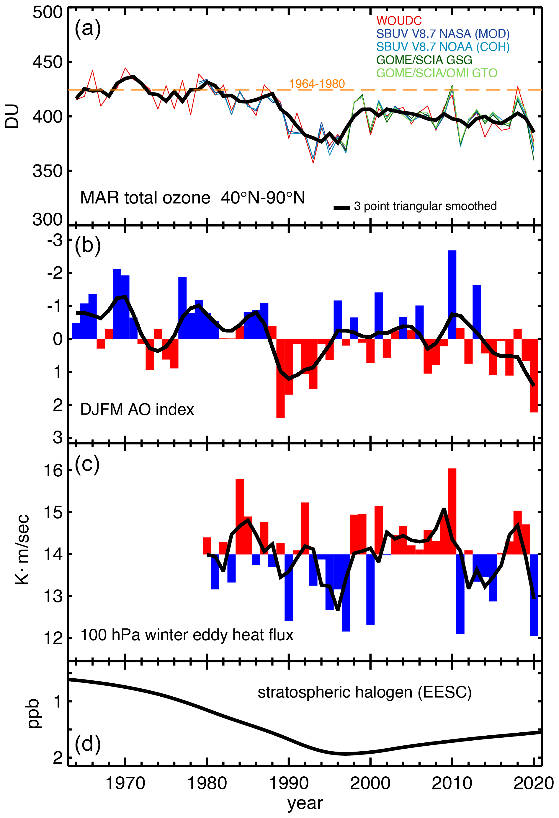
Figure 6(a) March NH total ozone (40–90∘ N) from the five bias-corrected merged datasets (coloured) and the smoothed median time series (thick black line). (b) DJFM Arctic Oscillation (AO) index. Black lines shows the three-point triangular smoothed time series. Note the inverted y scale. (c) 100 hPa winter eddy heat flux September to March average (BDCn proxy), with the black line showing the three-point triangular smoothed time series. (d) Inverted stratospheric halogen time series in parts per billion (ppb), representative of middle latitudes (Newman et al., 2007).
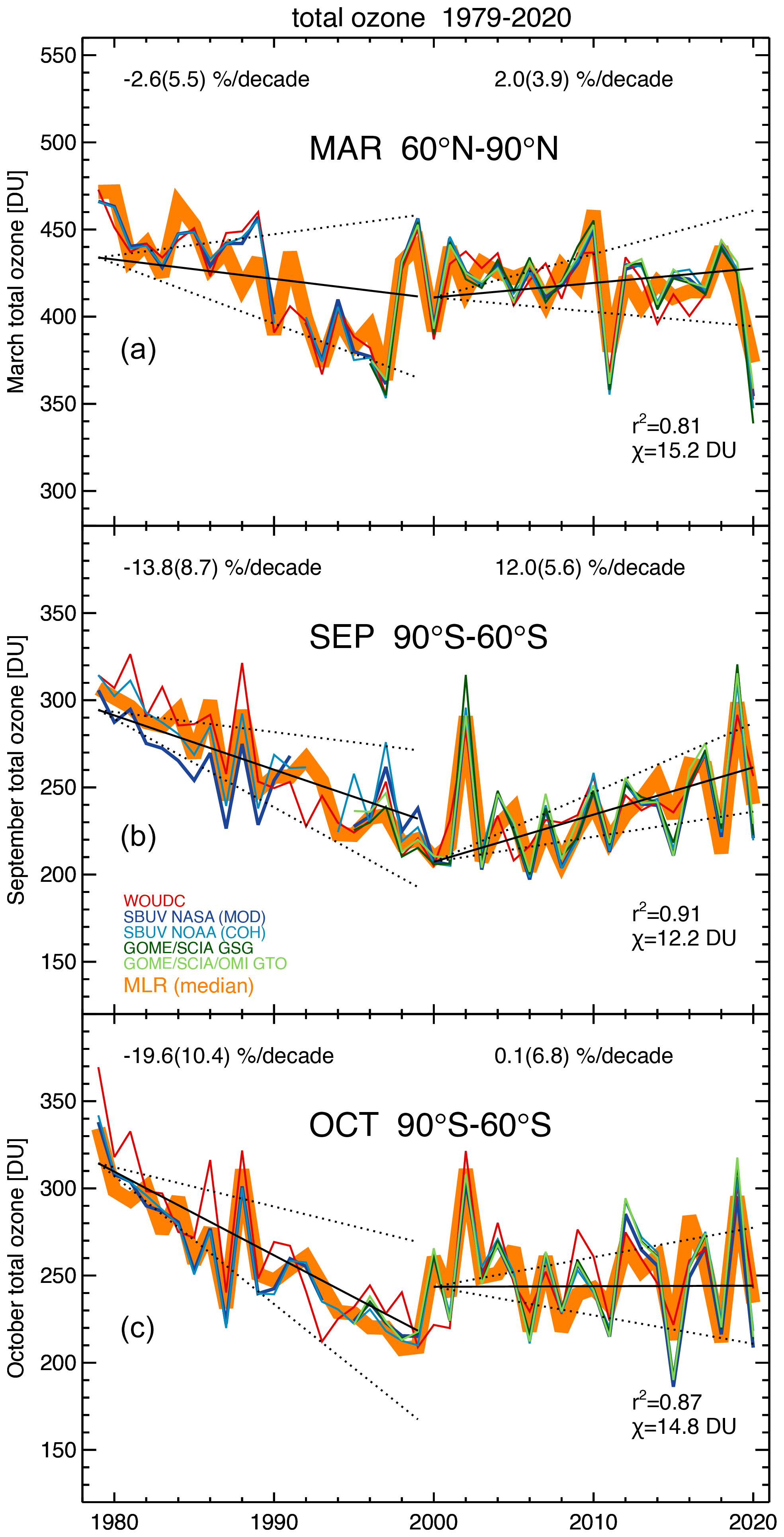
Figure 7Polar ozone trends derived from the full MLR applied to the median time series. (a) March 60–90∘ N, (b) September, and (c) October 60–90∘ S. See Fig. 1 for more details.
In the NH, the BDC and AO mostly contribute to ozone variability. Interestingly, there is an influence from the BDC from one hemisphere to the other in both directions. BDCn results in opposite responses in the tropics and NH extratropics. This is expected from the planetary waves driving the BDC, leading to ascent in the tropics (lower ozone) and descent in the polar region (higher ozone) (e.g. Randel et al., 2002; Weber et al., 2011). The correlation of ozone anomalies in the NH winter and spring to SH total ozone was reported by Fioletov and Shepherd (2003) and is believed to explain the positive response in SH total ozone. Somewhat surprising is the impact of the SH BDC on NH ozone with a negative ozone response, for which we have no explanation.
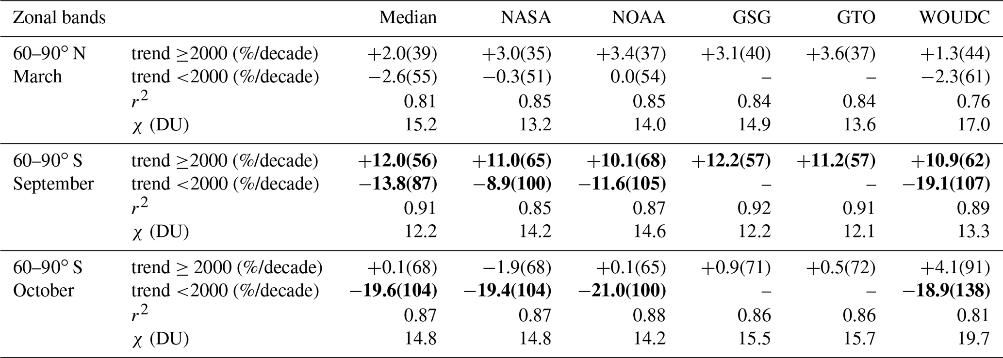
Table 5Polar total ozone trends in March (NH), September (SH), and October (SH) before and after 2000. Uncertainties are provided for 2σ, and trends in bold indicate statistical significance. r2 is the square Pearson correlation and χ the residual (see caption of Table 3). The results were obtained from the full MLR.
Bold numbers: statistical significance at 2σ.
The major volcanic eruption of Mt. Pinatubo in 1991 had a stronger impact on the NH, reducing ozone for several years after the event, while ozone advection apparently balanced the surface acid particle (aerosol)-related ozone losses in the SH (Schnadt Poberaj et al., 2011; Aquila et al., 2013; Dhomse et al., 2015). The second large major volcanic eruption from spring 1982 led to aerosol-related ozone loss in the tropics and NH, while surprisingly a positive ozone response in the SH is seen, possibly related to some atmospheric circulation changes compensating for chemical effects from the El Chichon eruption. In contrast to Mt. Pinatubo, which spread sulfuric acid particles into both hemispheres, enhanced aerosols from El Chichon were confined to lower latitudes in the NH (McCormick and Swissler, 1983), consistent with the region of negative ozone response shown in Fig. 5.
The main reason for stable ozone levels observed at NH mid-latitudes since 2000 was identified to stem from the balancing of the positive observed ODS-related trend by negative trends due to circulation changes and ozone transport (see Figs. 2 and 3). The change in the BDCn proxy and AO over the last 55 years is shown in Fig. 6, along with March total ozone northward of 40∘ N. The variability in the extratropical annual mean is usually dominated by the variability in winter and spring, where BDC maximizes in the seasonal cycle. Apart from the strong drop in ozone in the 1990s related to the major volcanic eruption and associated circulation changes, NH total ozone has been steadily declining over the last 55 years (about 25 DU). This decline is coherent with an overall positive shift of the AO index. A weakening of the BDC is also seen but appears less clear than for the AO.
A positive shift in the AO and a weakening of the BDC result in a strengthening of the polar vortex, which is associated with larger polar ozone losses (Lawrence et al., 2020). Hu et al. (2018) linked a recent strengthening of the stratospheric Arctic vortex in part to a warming of sea surface temperatures in the central northern Pacific. A downward trend in extratropical lower stratospheric ozone has been reported by Ball et al. (2018) that could be consistent with the total ozone observations. Other studies with many different ozone profile datasets did not show significant trends in the lower stratosphere due to very large variability and lower accuracy of the satellite data in this altitude region (Sofieva et al., 2017; Steinbrecht et al., 2017; Arosio et al., 2019).
Earlier signs of ozone recovery were observed in September above Antarctica (Solomon et al., 2016, W18). Now, with 4 more years of data, this recovery of about +12 %/decade remains robust (see Fig. 7b). During September, the Antarctic ozone hole size usually increases and reaches its maximum in late September and early October. In a typical Antarctic winter, ozone is completely destroyed in the lower stratosphere, which may explain why no recovery is yet observed in October over the polar cap (Fig. 7c). Several diagnostics clearly indicate a healing of Antarctic ozone as a consequence of the Montreal Protocol. Stone et al. (2021) show that the onset of the Antarctic ozone hole has been shifted to later dates despite the larger than average ozone holes observed in recent years (e.g. 2015 and 2020).
Figure 7a shows the March ozone time series above the Arctic, with ODS-related ozone trends not statistically different from zero. The trend results in the polar regions basically confirm the results from W18 and Langematz et al. (2018). Table 5 summarizes the polar trends for the individual datasets and the mean time series. Within the trend uncertainties, all datasets are in very good agreement.
We derived globally total ozone trends from five merged total ozone datasets using a multiple linear regression with independent linear trend (ILT) terms before and after the turnaround in stratospheric halogens in the middle 1990s (∼2000 in the polar regions). When properly accounting for dynamical changes via atmospheric circulation and transport, these retrieved trends may be directly related to changes in the stratospheric halogens (and ODSs) as a response to the Montreal Protocol and its amendments phasing out ozone-depleting substances.
For the near-global average we see small ODS-related trends of about +0.5 %/decade, with main contributions from the extratropics in both hemispheres. The ratio of ozone trends after and before the turnaround year is in very good agreement with the trend ratios in stratospheric halogens or ODSs.
In the tropics, trends are not statistically different from zero. In line with earlier observations (Solomon et al., 2016, W18), polar ozone recovery has been only identified in September above Antarctica, which is connected to the observed delay in the onset of the Antarctic ozone hole (Stone et al., 2021). In the Arctic, large interannual variability still prevents the detection of early signs of recovery.
Although we showed that ODS-related ozone recovery is evident at NH middle latitudes, the total ozone levels in the NH extratropics have been more or less stable since about 2000. Our regression results show that the positive ODS-related trend here is balanced by changes in ozone transport. A long-term positive drift in the AO index over the last 55 years is indicative of a strengthening of the Arctic vortex (Hu et al., 2018; Lawrence et al., 2020; von der Gathen et al., 2021) and reduced winter and spring transport of ozone into middle and high latitudes. This result may be consistent with the observed decline in lower stratospheric ozone in the extratropics as reported by Ball et al. (2018) and Wargan et al. (2018). They mainly attribute this decline to enhanced horizontal mixing with the tropical region, where lowermost stratospheric ozone decreases (Thompson et al., 2021). Other studies and datasets, however, have so far not confirmed the long-term extratropical decline in the lower stratosphere (Arosio et al., 2019; Steinbrecht et al., 2017; Sofieva et al., 2017), which may be in part due to the larger uncertainties of satellite observations in this altitude region. From chemistry–climate models, it is expected that with a strengthening of the BDC due to increasing GHGs, tropical ozone declines and extratropical ozone increases in the lower stratosphere (Dietmüller et al., 2021).
The supplement related to this article is available online at: https://doi.org/10.5194/acp-22-6843-2022-supplement.
MW designed the study, MW and CA carried out the analysis, and MCE, DL, JDW, SMF, VEF, and KT provided the updated observational and model datasets (see Table 1). All authors contributed to the drafting and revision of the paper.
At least one of the (co-)authors is a guest member of the editorial board of Atmospheric Chemistry and Physics for the special issue “Atmospheric ozone and related species in the early 2020s: latest results and trends (ACP/AMT inter-journal SI)”. The peer-review process was guided by an independent editor, and the authors also have no other competing interests to declare.
Publisher’s note: Copernicus Publications remains neutral with regard to jurisdictional claims in published maps and institutional affiliations.
This article is part of the special issue “Atmospheric ozone and related species in the early 2020s: latest results and trends (ACP/AMT inter-journal SI)”. It is not associated with a conference.
The financial support by various projects and institutions is gratefully acknowledged (see Financial support section). We thank the two reviewers for their very useful comments on our paper.
Melanie Coldewey-Egbers, Diego Loyola, and Carlo Arosio were supported
by the ESA Climate Change Initiative project, CCI+. Mark Weber, Carlo Arosio, and John P. Burrows were supported by the State of Bremen and from the OREGANO
project (ESA contract no. 4000137112/22/I-AG). Mark Weber was supported by the BMBF project Synopsys-Ozon (FKZ 03F0872B). Stacey M. Frith was
supported by the NASA Long Term Measurement of Ozone programme, WBS 479717.
The article processing charges for this open-access publication were covered by the University of Bremen.
This paper was edited by Michel Van Roozendael and reviewed by two anonymous referees.
Anderson, J., Russell, J. M., Solomon, S., and Deaver, L. E.: Halogen Occultation Experiment confirmation of stratospheric chlorine decreases in accordance with the Montreal Protocol, J. Geophys. Res.-Atmos., 105, 4483–4490, https://doi.org/10.1029/1999JD901075, 2000. a
Aquila, V., Oman, L. D., Stolarski, R., Douglass, A. R., and Newman, P. A.: The response of ozone and nitrogen dioxide to the eruption of Mt. Pinatubo at southern and northern midlatitudes, J. Atmos. Sci., 70, 894–900, https://doi.org/10.1175/JAS-D-12-0143.1, 2013. a
Arosio, C., Rozanov, A., Malinina, E., Weber, M., and Burrows, J. P.: Merging of ozone profiles from SCIAMACHY, OMPS and SAGE II observations to study stratospheric ozone changes, Atmos. Meas. Tech., 12, 2423–2444, https://doi.org/10.5194/amt-12-2423-2019, 2019. a, b
Atkinson, R. J., Matthews, W. A., Newman, P. A., and Plumb, R. A.: Evidence of the mid-latitude impact of Antarctic ozone depletion, Nature, 340, 290–294, https://doi.org/10.1038/340290a0, 1989. a
Baldwin, M. P., Gray, L. J., Dunkerton, T. J., Hamilton, K., Haynes, P. H., Randel, W. J., Holton, J. R., Alexander, M. J., Hirota, I., Horinouchi, T., Jones, D. B. A., Kinnersley, J. S., Marquardt, C., Sato, K., and Takahashi, M.: The Quasi-Biennial Oscillation, Rev. Geophys., 39, 179–229, https://doi.org/10.1029/1999RG000073, 2001. a
Ball, W. T., Alsing, J., Mortlock, D. J., Staehelin, J., Haigh, J. D., Peter, T., Tummon, F., Stübi, R., Stenke, A., Anderson, J., Bourassa, A., Davis, S. M., Degenstein, D., Frith, S., Froidevaux, L., Roth, C., Sofieva, V., Wang, R., Wild, J., Yu, P., Ziemke, J. R., and Rozanov, E. V.: Evidence for a continuous decline in lower stratospheric ozone offsetting ozone layer recovery, Atmos. Chem. Phys., 18, 1379–1394, https://doi.org/10.5194/acp-18-1379-2018, 2018. a, b
Bhartia, P. K., McPeters, R. D., Flynn, L. E., Taylor, S., Kramarova, N. A., Frith, S., Fisher, B., and DeLand, M.: Solar Backscatter UV (SBUV) total ozone and profile algorithm, Atmos. Meas. Tech., 6, 2533–2548, https://doi.org/10.5194/amt-6-2533-2013, 2013. a
Bloomer, B. J., Vinnikov, K. Y., and Dickerson, R. R.: Changes in seasonal and diurnal cycles of ozone and temperature in the eastern U.S., Atmos. Environ., 44, 2543–2551, https://doi.org/10.1016/j.atmosenv.2010.04.031, 2010. a
Bourassa, A. E., Degenstein, D. A., Randel, W. J., Zawodny, J. M., Kyrölä, E., McLinden, C. A., Sioris, C. E., and Roth, C. Z.: Trends in stratospheric ozone derived from merged SAGE II and Odin-OSIRIS satellite observations, Atmos. Chem. Phys., 14, 6983–6994, https://doi.org/10.5194/acp-14-6983-2014, 2014. a
Bourassa, A. E., Roth, C. Z., Zawada, D. J., Rieger, L. A., McLinden, C. A., and Degenstein, D. A.: Drift-corrected Odin-OSIRIS ozone product: algorithm and updated stratospheric ozone trends, Atmos. Meas. Tech., 11, 489–498, https://doi.org/10.5194/amt-11-489-2018, 2018. a
Bowman, K. P.: Global Patterns of the Quasi-biennial Oscillation in Total Ozone, J. Atmos. Sci., 46, 3328–3343, https://doi.org/10.1175/1520-0469(1989)046<3328:GPOTQB>2.0.CO;2, 1989. a
Bozhkova, V., Liudchik, A., and Umreiko, S.: Long-term trends of total ozone content over mid-latitudes of the Northern Hemisphere, Int. J. Remote Sens., 40, 5216–5229, https://doi.org/10.1080/01431161.2019.1579384, 2019. a, b
Braesicke, P., Neu, J., Fioletov, V., Godin-Beekmann, S., Hubert, D., Petropavlovskikh, I., Shiotani, M., and Sinnhuber, B.-M.: Update on Global Ozone: Past, Present, and Future, in: Scientific Assessment of Ozone Depletion: 2018, World Meteorological Organization, Global Ozone Research and Monitoring Project – Report No. 58, chap. 3, World Meteorological Organization/UNEP, https://public.wmo.int/en/resources/library/scientific-assessment-of-ozone-depletion-2018 (last access: 19 May 2022), 2018. a, b, c
Chehade, W., Weber, M., and Burrows, J. P.: Total ozone trends and variability during 1979–2012 from merged data sets of various satellites, Atmos. Chem. Phys., 14, 7059–7074, https://doi.org/10.5194/acp-14-7059-2014, 2014. a
Chiou, E. W., Bhartia, P. K., McPeters, R. D., Loyola, D. G., Coldewey-Egbers, M., Fioletov, V. E., Van Roozendael, M., Spurr, R., Lerot, C., and Frith, S. M.: Comparison of profile total ozone from SBUV (v8.6) with GOME-type and ground-based total ozone for a 16-year period (1996 to 2011), Atmos. Meas. Tech., 7, 1681–1692, https://doi.org/10.5194/amt-7-1681-2014, 2014. a, b
Chubachi, S.: Preliminary results of ozone observations at Syowa Station from February 1982 to January 1983, in: Proc. Sixth Symposium on Polar Meteorology and Glaciology, edited by: Kusunoki, K., vol. 34 of Mem. National Institute of Polar Research Special Issue, 13–19, 1984. a
Coldewey-Egbers, M., Weber, M., Lamsal, L. N., de Beek, R., Buchwitz, M., and Burrows, J. P.: Total ozone retrieval from GOME UV spectral data using the weighting function DOAS approach, Atmos. Chem. Phys., 5, 1015–1025, https://doi.org/10.5194/acp-5-1015-2005, 2005. a
Coldewey-Egbers, M., Loyola, D. G., Koukouli, M., Balis, D., Lambert, J.-C., Verhoelst, T., Granville, J., van Roozendael, M., Lerot, C., Spurr, R., Frith, S. M., and Zehner, C.: The GOME-type Total Ozone Essential Climate Variable (GTO-ECV) data record from the ESA Climate Change Initiative, Atmos. Meas. Tech., 8, 3923–3940, https://doi.org/10.5194/amt-8-3923-2015, 2015. a
Coldewey-Egbers, M., Loyola, D. G., Lerot, C., and Van Roozendael, M.: Global, regional and seasonal analysis of total ozone trends derived from the 1995–2020 GTO-ECV climate data record, Atmos. Chem. Phys. Discuss. [preprint], https://doi.org/10.5194/acp-2021-1047, in review, 2022. a, b, c, d
DeLand, M. T., Taylor, S. L., Huang, L. K., and Fisher, B. L.: Calibration of the SBUV version 8.6 ozone data product, Atmos. Meas. Tech., 5, 2951–2967, https://doi.org/10.5194/amt-5-2951-2012, 2012. a, b
Dhomse, S., Weber, M., Wohltmann, I., Rex, M., and Burrows, J. P.: On the possible causes of recent increases in northern hemispheric total ozone from a statistical analysis of satellite data from 1979 to 2003, Atmos. Chem. Phys., 6, 1165–1180, https://doi.org/10.5194/acp-6-1165-2006, 2006. a, b, c
Dhomse, S. S., Chipperfield, M. P., Feng, W., Hossaini, R., Mann, G. W., and Santee, M. L.: Revisiting the hemispheric asymmetry in midlatitude ozone changes following the Mount Pinatubo eruption: A 3-D model study, Geophys. Res. Lett., 42, 3038–3047, https://doi.org/10.1002/2015GL063052, 2015. a, b
Dhomse, S. S., Chipperfield, M. P., Feng, W., Hossaini, R., Mann, G. W., Santee, M. L., and Weber, M.: A single-peak-structured solar cycle signal in stratospheric ozone based on Microwave Limb Sounder observations and model simulations, Atmos. Chem. Phys., 22, 903–916, https://doi.org/10.5194/acp-22-903-2022, 2022. a
Dietmüller, S., Garny, H., Eichinger, R., and Ball, W. T.: Analysis of recent lower-stratospheric ozone trends in chemistry climate models, Atmos. Chem. Phys., 21, 6811–6837, https://doi.org/10.5194/acp-21-6811-2021, 2021. a
Eyring, V., Arblaster, J. M., Cionni, I., Sedláček, J., Perlwitz, J., Young, P. J., Bekki, S., Bergmann, D., Cameron-Smith, P., Collins, W. J., Faluvegi, G., Gottschaldt, K.-D., Horowitz, L. W., Kinnison, D. E., Lamarque, J.-F., Marsh, D. R., Saint-Martin, D., Shindell, D. T., Sudo, K., Szopa, S., and Watanabe, S.: Long-term ozone changes and associated climate impacts in CMIP5 simulations, J. Geophys. Res.-Atmos., 118, 5029–5060, https://doi.org/10.1002/jgrd.50316, 2013. a, b
Farman, J. C., Gardiner, B. G., and Shanklin, J. D.: Large losses of total ozone in Antarctica reveal seasonal ClOx NOx interaction, Nature, 315, 207–210, https://doi.org/10.1038/315207a0, 1985. a
Fioletov, V. E. and Shepherd, T. G.: Seasonal persistence of midlatitude total ozone anomalies, Geophys. Res. Lett., 30, 1417, https://doi.org/10.1029/2002GL016739, 2003. a
Fioletov, V. E., Bodeker, G. E., Miller, A. J., McPeters, R. D., and Stolarski, R.: Global and zonal total ozone variations estimated from ground-based and satellite measurements: 1964–2000, J. Geophys. Res., 107, 4647, https://doi.org/10.1029/2001JD001350, 2002. a, b
Fioletov, V. E., Labow, G., Evans, R., Hare, E. W., Köhler, U., McElroy, C. T., Miyagawa, K., Redondas, A., Savastiouk, V., Shalamyansky, A. M., Staehelin, J., Vanicek, K., and Weber, M.: Performance of the ground-based total ozone network assessed using satellite data, J. Geophys. Res., 113, D14313, https://doi.org/10.1029/2008JD009809, 2008. a
Frith, S., Kramarova, N., Bhartia, P., Huang, L.-K., Ziemke, J., McPeters, R., Labow, G., Haffner, D., Stolarski, R., and DeLand, M.: Updates to the Merged Ozone Data (MOD) total and profile ozone record based on V8.7 SBUV(/2) and V2.8 OMPS Nadir Profiler Data, Atmos. Meas. Tech., in preparation, 2022. a
Frith, S. M., Kramarova, N. A., Stolarski, R. S., McPeters, R. D., Bhartia, P. K., and Labow, G. J.: Recent changes in total column ozone based on the SBUV Version 8.6 Merged Ozone Data Set, J. Geophys. Res.-Atmos., 119, 9735–9751, https://doi.org/10.1002/2014JD021889, 2014. a
Frith, S. M., Bhartia, P. K., Oman, L. D., Kramarova, N. A., McPeters, R. D., and Labow, G. J.: Model-based climatology of diurnal variability in stratospheric ozone as a data analysis tool, Atmos. Meas. Tech., 13, 2733–2749, https://doi.org/10.5194/amt-13-2733-2020, 2020. a
Fusco, A. C. and Salby, M. L.: Interannual Variations of Total Ozone and Their Relationship to Variations of Planetary Wave Activity, J. Climate, 12, 1619–1629, https://doi.org/10.1175/1520-0442(1999)012<1619:IVOTOA>2.0.CO;2, 1999. a, b
Garane, K., Lerot, C., Coldewey-Egbers, M., Verhoelst, T., Koukouli, M. E., Zyrichidou, I., Balis, D. S., Danckaert, T., Goutail, F., Granville, J., Hubert, D., Keppens, A., Lambert, J.-C., Loyola, D., Pommereau, J.-P., Van Roozendael, M., and Zehner, C.: Quality assessment of the Ozone_cci Climate Research Data Package (release 2017) – Part 1: Ground-based validation of total ozone column data products, Atmos. Meas. Tech., 11, 1385–1402, https://doi.org/10.5194/amt-11-1385-2018, 2018. a, b
Garane, K., Koukouli, M.-E., Verhoelst, T., Lerot, C., Heue, K.-P., Fioletov, V., Balis, D., Bais, A., Bazureau, A., Dehn, A., Goutail, F., Granville, J., Griffin, D., Hubert, D., Keppens, A., Lambert, J.-C., Loyola, D., McLinden, C., Pazmino, A., Pommereau, J.-P., Redondas, A., Romahn, F., Valks, P., Van Roozendael, M., Xu, J., Zehner, C., Zerefos, C., and Zimmer, W.: TROPOMI/S5P total ozone column data: global ground-based validation and consistency with other satellite missions, Atmos. Meas. Tech., 12, 5263–5287, https://doi.org/10.5194/amt-12-5263-2019, 2019. a
Harris, N. R. P., Kyrö, E., Staehelin, J., Brunner, D., Andersen, S.-B., Godin-Beekmann, S., Dhomse, S., Hadjinicolaou, P., Hansen, G., Isaksen, I., Jrrar, A., Karpetchko, A., Kivi, R., Knudsen, B., Krizan, P., Lastovicka, J., Maeder, J., Orsolini, Y., Pyle, J. A., Rex, M., Vanicek, K., Weber, M., Wohltmann, I., Zanis, P., and Zerefos, C.: Ozone trends at northern mid- and high latitudes – a European perspective, Ann. Geophys., 26, 1207–1220, https://doi.org/10.5194/angeo-26-1207-2008, 2008. a, b
Harris, N. R. P., Hassler, B., Tummon, F., Bodeker, G. E., Hubert, D., Petropavlovskikh, I., Steinbrecht, W., Anderson, J., Bhartia, P. K., Boone, C. D., Bourassa, A., Davis, S. M., Degenstein, D., Delcloo, A., Frith, S. M., Froidevaux, L., Godin-Beekmann, S., Jones, N., Kurylo, M. J., Kyrölä, E., Laine, M., Leblanc, S. T., Lambert, J.-C., Liley, B., Mahieu, E., Maycock, A., de Mazière, M., Parrish, A., Querel, R., Rosenlof, K. H., Roth, C., Sioris, C., Staehelin, J., Stolarski, R. S., Stübi, R., Tamminen, J., Vigouroux, C., Walker, K. A., Wang, H. J., Wild, J., and Zawodny, J. M.: Past changes in the vertical distribution of ozone – Part 3: Analysis and interpretation of trends, Atmos. Chem. Phys., 15, 9965–9982, https://doi.org/10.5194/acp-15-9965-2015, 2015. a
Hegglin, M., Lamarque, J.-F., Duncan, B., Eyring, V. Gettelman, A., Hess, P., Myhre, G., Nagashima, T., Plummer, D., Ryerson, T., Shepherd, T., and Waugh, D.: Report on the IGAC/SPARC Chemistry-Climate Model Initiative (CCMI) 2015 Science workshop, SPARC Newsletter, http://www.sparc-climate.org/wp-content/uploads/sites/5/2017/12/SPARCnewsletter_No46_Jan2016_web.pdf (last access: 19 May 2022), 46, 37–42, 2016. a
Hersbach, H., Bell, B., Berrisford, P., Hirahara, S., Horányi, A., Muñoz‐Sabater, J., Nicolas, J., Peubey, C., Radu, R., Schepers, D., Simmons, A., Soci, C., Abdalla, S., Abellan, X., Balsamo, G., Bechtold, P., Biavati, G., Bidlot, J., Bonavita, M., Chiara, G., Dahlgren, P., Dee, D., Diamantakis, M., Dragani, R., Flemming, J., Forbes, R., Fuentes, M., Geer, A., Haimberger, L., Healy, S., Hogan, R. J., Hólm, E., Janisková, M., Keeley, S., Laloyaux, P., Lopez, P., Lupu, C., Radnoti, G., Rosnay, P., Rozum, I., Vamborg, F., Villaume, S., and Thépaut, J.: The ERA5 global reanalysis, Q. J. Roy. Meteor. Soc., 146, 1999–2049, https://doi.org/10.1002/qj.3803, 2020. a
Hu, D., Guan, Z., Tian, W., and Ren, R.: Recent strengthening of the stratospheric Arctic vortex response to warming in the central North Pacific, Nat. Comm., 9, 1697, https://doi.org/10.1038/s41467-018-04138-3, 2018. a, b
Kiesewetter, G., Sinnhuber, B.-M., Weber, M., and Burrows, J. P.: Attribution of stratospheric ozone trends to chemistry and transport: a modelling study, Atmos. Chem. Phys., 10, 12073–12089, https://doi.org/10.5194/acp-10-12073-2010, 2010. a
Kramarova, N., Bhartia, P., Huang, L.-K., Ziemke, J., Frith, S. M., McPeters, R., Labow, G., Haffner, D., Stolarski, R., and DeLand, M.: A new approach to cross-calibrate satellite instruments, Atmos. Meas. Tech., in preparation, 2022. a, b
Kramarova, N. A., Frith, S. M., Bhartia, P. K., McPeters, R. D., Taylor, S. L., Fisher, B. L., Labow, G. J., and DeLand, M. T.: Validation of ozone monthly zonal mean profiles obtained from the version 8.6 Solar Backscatter Ultraviolet algorithm, Atmos. Chem. Phys., 13, 6887–6905, https://doi.org/10.5194/acp-13-6887-2013, 2013. a
Krzyścin, J. W. and Baranowski, D. B.: Signs of the ozone recovery based on multi sensor reanalysis of total ozone for the period 1979–2017, Atmos. Environ., 199, 334–344, https://doi.org/10.1016/j.atmosenv.2018.11.050, 2019. a, b
Langematz, U., Tully, M. B., Calvo, N., Dameris, M., de Laat, A. T. J., Klekociuk, A., Müller, R., and Young, P.: Update on Polar Stratospheric Ozone: Past, Present, and Future, in: Scientific Assessment of Ozone Depletion: 2018, World Meteorological Organization, Global Ozone Research and Monitoring Project – Report No. 58, chap. 4, World Meteorological Organization/UNEP, https://public.wmo.int/en/resources/library/scientific-assessment-of-ozone-depletion-2018 (last access: 19 May 2022), 2018. a
Lawrence, Z. D., Perlwitz, J., Butler, A. H., Manney, G. L., Newman, P. A., Lee, S. H., and Nash, E. R.: The remarkably strong Arctic stratospheric polar vortex of winter 2020: Links to record-breaking Arctic Oscillation and ozone loss, J. Geophys. Res.-Atmos., 125, e2020JD033271, https://doi.org/10.1029/2020JD033271, 2020. a, b
Lerot, C., Van Roozendael, M., Spurr, R., Loyola, D., Coldewey-Egbers, M., Kochenova, S., van Gent, J., Koukouli, M., Balis, D., Lambert, J.-C., Granville, J., and Zehner, C.: Homogenized total ozone data records from the European sensors GOME/ERS-2, SCIAMACHY/Envisat, and GOME-2/MetOp-A, J. Geophys. Res.-Atmos., 119, 1639–1662, https://doi.org/10.1002/2013JD020831, 2014. a
Mäder, J. A., Staehelin, J., Brunner, D., Stahel, W. A., Wohltmann, I., and Peter, T.: Statistical modeling of total ozone: Selection of appropriate explanatory variables, J. Geophys. Res., 112, D11108, https://doi.org/10.1029/2006JD007694, 2007. a
Mäder, J. A., Staehelin, J., Peter, T., Brunner, D., Rieder, H. E., and Stahel, W. A.: Evidence for the effectiveness of the Montreal Protocol to protect the ozone layer, Atmos. Chem. Phys., 10, 12161–12171, https://doi.org/10.5194/acp-10-12161-2010, 2010. a
McCormick, M. P. and Swissler, T. J.: Stratospheric aerosol mass and latitudinal distribution of the El Chichon eruption cloud for October 1982, Geophys. Res. Lett., 10, 877–880, https://doi.org/10.1029/GL010i009p00877, 1983. a
Millard, G. A., Lee, A. M., and Pyle, J. A.: A model study of the connection between polar and midlatitude ozone loss in the Northern Hemisphere lower stratosphere, J. Geophys. Res.-Atmos., 107, 1–12, https://doi.org/10.1029/2001JD000899, 2002. a
Mills, M. J., Schmidt, A., Easter, R., Solomon, S., Kinnison, D. E., Ghan, S. J., Neely, R. R., Marsh, D. R., Conley, A., Bardeen, C. G., and Gettelman, A.: Global volcanic aerosol properties derived from emissions, 1990–2014, using CESM1(WACCM), J. Geophys. Res.-Atmos., 121, 2332–2348, https://doi.org/10.1002/2015JD024290, 2016. a, b
Morgenstern, O., Hegglin, M. I., Rozanov, E., O'Connor, F. M., Abraham, N. L., Akiyoshi, H., Archibald, A. T., Bekki, S., Butchart, N., Chipperfield, M. P., Deushi, M., Dhomse, S. S., Garcia, R. R., Hardiman, S. C., Horowitz, L. W., Jöckel, P., Josse, B., Kinnison, D., Lin, M., Mancini, E., Manyin, M. E., Marchand, M., Marécal, V., Michou, M., Oman, L. D., Pitari, G., Plummer, D. A., Revell, L. E., Saint-Martin, D., Schofield, R., Stenke, A., Stone, K., Sudo, K., Tanaka, T. Y., Tilmes, S., Yamashita, Y., Yoshida, K., and Zeng, G.: Review of the global models used within phase 1 of the Chemistry–Climate Model Initiative (CCMI), Geosci. Model Dev., 10, 639–671, https://doi.org/10.5194/gmd-10-639-2017, 2017. a
Naujokat, B.: An update of the observed Quasi-Biennial Oscillation of the stratospheric winds over the tropics, J. Atmos. Sci., 43, 1873–1877, https://doi.org/10.1175/1520-0469(1986)043<1873:AUOTOQ>2.0.CO;2, 1986. a
Newman, P. A., Nash, E. R., Kawa, S. R., Montzka, S. A., and Schauffler, S. M.: When will the Antarctic ozone hole recover?, Geophys. Res. Lett., 33, L12814, https://doi.org/10.1029/2005GL025232, 2006. a
Newman, P. A., Daniel, J. S., Waugh, D. W., and Nash, E. R.: A new formulation of equivalent effective stratospheric chlorine (EESC), Atmos. Chem. Phys., 7, 4537–4552, https://doi.org/10.5194/acp-7-4537-2007, 2007. a, b, c, d
Orfanoz-Cheuquelaf, A., Rozanov, A., Weber, M., Arosio, C., Ladstätter-Weißenmayer, A., and Burrows, J. P.: Total ozone column from Ozone Mapping and Profiler Suite Nadir Mapper (OMPS-NM) measurements using the broadband weighting function fitting approach (WFFA), Atmos. Meas. Tech., 14, 5771–5789, https://doi.org/10.5194/amt-14-5771-2021, 2021. a
Randel, W. J., Wu, F., and Stolarski, R.: Changes in column ozone correlated with the stratospheric EP flux, J. Meteorol. Soc. Jpn., 80, 849–862, https://doi.org/10.2151/jmsj.80.849, 2002. a, b, c
Reinsel, G. C., Miller, A. J., Weatherhead, E. C., Flynn, L. E., Nagatani, R. M., Tiao, G. C., and Wuebbles, D. J.: Trend analysis of total ozone data for turnaround and dynamical contributions, J. Geophys. Res., 110, D16306, https://doi.org/10.1029/2004JD004662, 2005. a, b
Sato, M., Hansen, J. E., McCormick, M. P., and Pollack, J. B.: Stratospheric aerosol optical depths, 1850–1990, J. Geophys. Res., 98, 22987, https://doi.org/10.1029/93JD02553, 1993. a, b
Schnadt Poberaj, C., Staehelin, J., and Brunner, D.: Missing stratospheric ozone decrease at Southern Hemisphere middle latitudes after Mt. Pinatubo: A dynamical perspective, J. Atmos. Sci., 68, 1922–1945, https://doi.org/10.1175/JAS-D-10-05004.1, 2011. a, b
Snow, M., Weber, M., Machol, J., Viereck, R., and Richard, E.: Comparison of Magnesium II core-to-wing ratio observations during solar minimum 23/24, J. Space Weather Space Clim., 4, A04, https://doi.org/10.1051/swsc/2014001, 2014. a
Sofieva, V. F., Kyrölä, E., Laine, M., Tamminen, J., Degenstein, D., Bourassa, A., Roth, C., Zawada, D., Weber, M., Rozanov, A., Rahpoe, N., Stiller, G., Laeng, A., von Clarmann, T., Walker, K. A., Sheese, P., Hubert, D., van Roozendael, M., Zehner, C., Damadeo, R., Zawodny, J., Kramarova, N., and Bhartia, P. K.: Merged SAGE II, Ozone_cci and OMPS ozone profile dataset and evaluation of ozone trends in the stratosphere, Atmos. Chem. Phys., 17, 12533–12552, https://doi.org/10.5194/acp-17-12533-2017, 2017. a, b, c
Solomon, P., Barrett, J., Mooney, T., Connor, B., Parrish, A., and Siskind, D. E.: Rise and decline of active chlorine in the stratosphere, Geophys. Res. Lett., 33, L18807, https://doi.org/10.1029/2006GL027029, 2006. a
Solomon, S.: Stratospheric ozone depletion: A review of concepts and history, Rev. Geophys., 37, 275–316, https://doi.org/10.1029/1999RG900008, 1999. a
Solomon, S., Garcia, R. R., Rowland, F. S., and Wuebbles, D. J.: On the depletion of Antarctic ozone, Nature, 321, 755–758, https://doi.org/10.1038/321755a0, 1986. a
Solomon, S., Ivy, D. J., Kinnison, D., Mills, M. J., Neely, R. R., and Schmidt, A.: Emergence of healing in the Antarctic ozone layer, Science, 353, 269–274, https://doi.org/10.1126/science.aae0061, 2016. a, b
Staehelin, J., Harris, N. R. P., Appenzeller, C., and Eberhard, J.: Ozone trends: A review, Rev. Geophys., 39, 231–290, https://doi.org/10.1029/1999RG000059, 2001. a
Steinbrecht, W., Froidevaux, L., Fuller, R., Wang, R., Anderson, J., Roth, C., Bourassa, A., Degenstein, D., Damadeo, R., Zawodny, J., Frith, S., McPeters, R., Bhartia, P., Wild, J., Long, C., Davis, S., Rosenlof, K., Sofieva, V., Walker, K., Rahpoe, N., Rozanov, A., Weber, M., Laeng, A., von Clarmann, T., Stiller, G., Kramarova, N., Godin-Beekmann, S., Leblanc, T., Querel, R., Swart, D., Boyd, I., Hocke, K., Kämpfer, N., Maillard Barras, E., Moreira, L., Nedoluha, G., Vigouroux, C., Blumenstock, T., Schneider, M., García, O., Jones, N., Mahieu, E., Smale, D., Kotkamp, M., Robinson, J., Petropavlovskikh, I., Harris, N., Hassler, B., Hubert, D., and Tummon, F.: An update on ozone profile trends for the period 2000 to 2016, Atmos. Chem. Phys., 17, 10675–10690, https://doi.org/10.5194/acp-17-10675-2017, 2017. a, b, c
Stone, K. A., Solomon, S., Kinnison, D. E., and Mills, M. J.: On Recent Large Antarctic Ozone Holes and Ozone Recovery Metrics, Geophys. Res. Lett., 48, e2021GL095232, https://doi.org/10.1029/2021GL095232, 2021. a, b
Thompson, A. M., Stauffer, R. M., Wargan, K., Witte, J. C., Kollonige, D. E., and Ziemke, J. R.: Regional and Seasonal Trends in Tropical Ozone From SHADOZ Profiles: Reference for Models and Satellite Products, J. Geophys. Res.-Atmos., 126, e2021JD034691, https://doi.org/10.1029/2021JD034691, 2021. a
Tummon, F., Hassler, B., Harris, N. R. P., Staehelin, J., Steinbrecht, W., Anderson, J., Bodeker, G. E., Bourassa, A., Davis, S. M., Degenstein, D., Frith, S. M., Froidevaux, L., Kyrölä, E., Laine, M., Long, C., Penckwitt, A. A., Sioris, C. E., Rosenlof, K. H., Roth, C., Wang, H.-J., and Wild, J.: Intercomparison of vertically resolved merged satellite ozone data sets: interannual variability and long-term trends, Atmos. Chem. Phys., 15, 3021–3043, https://doi.org/10.5194/acp-15-3021-2015, 2015. a
van der A, R. J., Allaart, M. A. F., and Eskes, H. J.: Extended and refined multi sensor reanalysis of total ozone for the period 1970–2012, Atmos. Meas. Tech., 8, 3021–3035, https://doi.org/10.5194/amt-8-3021-2015, 2015. a
von der Gathen, P., Kivi, R., Wohltmann, I., Salawitch, R. J., and Rex, M.: Climate change favours large seasonal loss of Arctic ozone, Nature Commun., 12, 3886, https://doi.org/10.1038/s41467-021-24089-6, 2021. a
Vyushin, D. I., Fioletov, V. E., and Shepherd, T. G.: Impact of long-range correlations on trend detection in total ozone, J. Geophys. Res., 112, D14307, https://doi.org/10.1029/2006JD008168, 2007. a
Wargan, K., Orbe, C., Pawson, S., Ziemke, J. R., Oman, L. D., Olsen, M. A., Coy, L., and Emma Knowland, K.: Recent Decline in Extratropical Lower Stratospheric Ozone Attributed to Circulation Changes, Geophys. Res. Lett., 45, 5166–5176, https://doi.org/10.1029/2018GL077406, 2018. a
Weatherhead, E. C., Reinsel, G. C., Tiao, G. C., Jackman, C. H., Bishop, L., Frith, S. M. H., DeLuisi, J., Keller, T., Oltmans, S. J., Fleming, E. L., Wuebbles, D. J., Kerr, J. B., Miller, A. J., Herman, J., McPeters, R., Nagatani, R. M., and Frederick, J. E.: Detecting the recovery of total column ozone, J. Geophys. Res.-Atmos., 105, 22201–22210, https://doi.org/10.1029/2000JD900063, 2000. a
Weber, M., Lamsal, L. N., Coldewey-Egbers, M., Bramstedt, K., and Burrows, J. P.: Pole-to-pole validation of GOME WFDOAS total ozone with groundbased data, Atmos. Chem. Phys., 5, 1341–1355, https://doi.org/10.5194/acp-5-1341-2005, 2005. a
Weber, M., Dikty, S., Burrows, J. P., Garny, H., Dameris, M., Kubin, A., Abalichin, J., and Langematz, U.: The Brewer-Dobson circulation and total ozone from seasonal to decadal time scales, Atmos. Chem. Phys., 11, 11221–11235, https://doi.org/10.5194/acp-11-11221-2011, 2011. a, b, c, d
Weber, M., Coldewey-Egbers, M., Fioletov, V. E., Frith, S. M., Wild, J. D., Burrows, J. P., Long, C. S., and Loyola, D.: Total ozone trends from 1979 to 2016 derived from five merged observational datasets – the emergence into ozone recovery, Atmos. Chem. Phys., 18, 2097–2117, https://doi.org/10.5194/acp-18-2097-2018, 2018. a, b, c, d, e
Weber, M., Steinbrecht, W., Arosio, C., van der A, R., Frith, S. M., Anderson, J., Coldewey-Egbers, M., Davis, S., Degenstein, D., Fioletov, V. E., Froidevaux, L., Hubert, D., Loyola, D., Rozanov, A., Roth, C., Sofieva, V., Tourpali, K., Wang, R., and Wild, J. D.: Global Climate Stratospheric ozone in “State of the Climate in 2020”, B. Am. Meteorol. Soc., 102, 92–95, https://doi.org/10.1175/BAMS-D-21-0098.1, 2021. a
Wolter, K. and Timlin, M. S.: El Niño/Southern Oscillation behaviour since 1871 as diagnosed in an extended multivariate ENSO index (MEI.ext), Int. J. Clim., 31, 1074–1087, https://doi.org/10.1002/joc.2336, 2011. a
Ziemke, J. R., Labow, G. J., Kramarova, N. A., McPeters, R. D., Bhartia, P. K., Oman, L. D., Frith, S. M., and Haffner, D. P.: A global ozone profile climatology for satellite retrieval algorithms based on Aura MLS measurements and the MERRA-2 GMI simulation, Atmos. Meas. Tech., 14, 6407–6418, https://doi.org/10.5194/amt-14-6407-2021, 2021. a
- Abstract
- Introduction
- Total ozone datasets
- Multiple linear regression
- Total ozone trends in broad zonal bands
- Latitude-dependent total ozone trends
- Trends in polar spring
- Summary and conclusions
- Data availability
- Author contributions
- Competing interests
- Disclaimer
- Special issue statement
- Acknowledgements
- Financial support
- Review statement
- References
- Supplement