The 2019 methane budget and uncertainties at 1° resolution and each country through Bayesian integration Of GOSAT total column methane data and a priori inventory estimates

We use optimal estimation (OE) to quantify methane fluxes based on total column CH₄ data from the Greenhouse Gases Observing Satellite (GOSAT) and the GEOS-Chem global chemistry transport model. We then project these fluxes to emissions by sector at 1^∘ resolution and then to each country using a new Bayesian algorithm that accounts for prior and posterior uncertainties in the methane emissions. These estimates are intended as a pilot dataset for the global stock take in support of the Paris Agreement. However, differences between the emissions reported here and widely used bottom-up inventories should be used as a starting point for further research because of potential systematic errors of these satellite-based emissions estimates. We find that agricultural and waste emissions are ∼ 263 ± 24 Tg CH₄ yr⁻¹, anthropogenic fossil emissions are 82 ± 12 Tg CH₄ yr⁻¹, and natural wetland/aquatic emissions are 180 ± 10 Tg CH₄ yr⁻¹. These estimates are consistent with previous inversions based on GOSAT data and the GEOS-Chem model. In addition, anthropogenic fossil estimates are consistent with those reported to the United Nations Framework Convention on Climate Change (80.4 Tg CH₄ yr⁻¹ for 2019). Alternative priors can be easily tested with our new Bayesian approach (also known as prior swapping) to determine their impact on posterior emissions estimates. We use this approach by swapping to priors that include much larger aquatic emissions and fossil emissions (based on isotopic evidence) and find little impact on our posterior fluxes. This indicates that these alternative inventories are inconsistent with our remote sensing estimates and also that the posteriors reported here are due to the observing and flux inversion system and not uncertainties in the prior inventories. We find that total emissions for approximately 57 countries can be resolved with this observing system based on the degrees-of-freedom for signal metric (DOFS > 1.0) that can be calculated with our Bayesian flux estimation approach. Below a DOFS of 0.5, estimates for country total emissions are more weighted to our choice of prior inventories. The top five emitting countries (Brazil, China, India, Russia, USA) emit about half of the global anthropogenic budget, similar to our choice of prior emissions but with the posterior emissions shifted towards the agricultural sector and less towards fossil emissions, consistent with our global posterior results. Our results suggest remote-sensing-based estimates of methane emissions can be substantially different (although within uncertainty) than bottom-up inventories, isotopic evidence, or estimates based on sparse in situ data, indicating a need for further studies reconciling these different approaches for quantifying the methane budget. Higher-resolution fluxes calculated from upcoming satellite or aircraft data such as the Tropospheric Monitoring Instrument (TROPOMI) and those in formulation such as the Copernicus CO₂M, MethaneSat, or Carbon Mapper can be incorporated into our Bayesian estimation framework for the purpose of reducing uncertainty and improving the spatial resolution and sectoral attribution of subsequent methane emissions estimates.

1 Introduction

1.1 Background on atmospheric methane

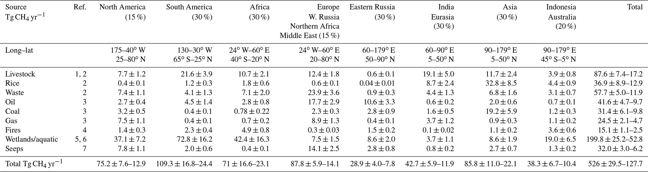
Atmospheric methane (CH₄) is the second-most important anthropogenic greenhouse gas behind carbon dioxide (CO₂) and a contributor to poor surface air quality as it is an ozone precursor. Atmospheric methane has increased by nearly a factor of 3 over its pre-industrial values, largely due to anthropogenic emissions (e.g., Dlugokencky et al., 2011; Ciais et al., 2013, and references therein). Over the last 2 decades, methane has been increasing but for reasons that are still being assessed, although recent studies provide evidence that it is due to a combination of fossil and agricultural emissions with some role due to variations in the atmospheric sink of methane (e.g., Schaefer et al., 2016; Worden et al., 2017; Turner et al., 2019; Zhang et al., 2021). However, it is unclear which regions and which sectors are the cause of changes in atmospheric methane over the last 20 years because of substantial uncertainties in all components of the methane budget (Kirschke et al., 2013; Janssens-Maenhout et al., 2019; Sanuois et al., 2020) from the global (Table 1) to local scale (Sect. 2). Methane has a relatively short lifetime of approximately 9 years, making it an attractive target for emissions reduction as a decline in emissions will have a rapid impact on net radiative forcing and corresponding atmospheric heating (e.g., Shindell et al., 2009; Ganesan et al., 2019; Turner et al., 2019). Hence there is significant interest in accurately quantifying methane emissions for identifying those emissions that can be efficiently reduced.

Table 1 Prior emissions and uncertainties are generated from various inventories or models (Sect. 2.3). Posterior emissions represent projection of satellite-based fluxes back to emissions while accounting for the prior emissions distribution and covariances (Sect. 2.2). We conservatively assume uncertainties are 100 % correlated, so that the total reported prior and posterior uncertainties are the sum of the individual uncertainties.

1.2 Global stock take

As part of the effort to reduce methane emissions and corresponding risk related to changes in climate, the Paris Agreement resulted in a framework by which countries provide an account of their emissions. A global stock take (GST) to track progress in emission reductions is conducted at 5-year intervals, beginning in 2023. To support the first GST, parties to the Paris Agreement are compiling inventories of GHG emissions and removals to inform their progress. Inventories are generally estimated using bottom-up approaches, in which emissions estimates are generally based on activity data and emissions factors. These bottom-up methods can provide precise and accurate emissions estimates when the activity data are well quantified and emissions factors are well understood. However, substantial uncertainties exist for emissions in many parts of the globe where these measurements are not rigorously made or tested across multiple sites. Even regions and emissions that are thought to be well measured can have significant differences between independent assessments and official reports; for example, Alvarez et al. (2018) demonstrate that 2015 oil and gas emissions are underestimated by the United States Environmental Protection Agency by about 60 %. These differences, if they are representative of emissions across the globe, indicate a need for an independent assessment of emissions and their uncertainties to better evaluate whether reported changes in emissions are in fact occurring or whether changes in the natural carbon cycle through wetlands and the methane sink are substantively affecting the atmospheric methane burden. Top-down estimates of methane emissions using atmospheric measurements provide an independent way of testing these inventories as observed methane concentrations are compared against expected concentrations that result from reported inventories. The objective of this paper is to demonstrate the use of satellite observations for testing and updating emissions by sector for use with the GST. While these top-down atmospheric methane budgets cannot replace the detailed activity reports used to generate bottom-up inventories, they can be combined with those bottom-up products to produce a more complete and transparent assessment of progress toward greenhouse gas emission reduction targets. They can also help determine whether the natural part of the methane budget is becoming a strong component of atmospheric methane increases. As discussed next, an important component of this assessment is the evaluation of uncertainties from both bottom-up inventories and in top-down approaches.

1.3 Overview of bottom-up emissions and uncertainties

Bottom-up uncertainties are calculated for the methane budget by comparison between independent methods or sources, evaluating multiple estimates from a single source, comparison between models and remote sensing data, and expert opinion. For example, Saunois et al. (2020) use a range of results from different studies to quantify uncertainty in the different sectors of the methane budget. However, these uncertainties are likely underestimated, as they suggest that total anthropogenic agricultural emissions, for example, are known to 10 % or better, whereas comparisons between different global inventories (e.g., Janssens-Maenhout et al., 2019) suggest a much larger range of estimates for the global totals (e.g., 129 to 219 Tg CH₄ yr⁻¹ for agriculture and 129 to 164 Tg CH₄ yr⁻¹ for fossil emissions). Uncertainties in national or regional total emissions are even more challenging to estimate, such that expert opinion is used: Janssens-Maenhout et al. (2019) suggest that Annex 1 (developed) countries have approximately 15 % uncertainty in reported fossil emissions, whereas Annex 2 countries have ∼ 30 % uncertainties, essentially asserting that less informed inventories have double the uncertainty of better informed emissions. Wetland emissions, which comprise ∼ 30 %–45 % of the methane budget, also show significant differences of up to 40 % across wetland models (e.g., Melton et al., 2013; Poulter et al., 2017; Schwietzke et al., 2016), depending on region. An example of how these uncertainties are projected to the total methane budget for each of the main sectors is presented in Table 1 using the prior emissions and their uncertainties for the analysis discussed in this paper (Sect. 2.3).

However, recent studies challenge even these estimates of emission uncertainties; emissions for lakes and rivers could be as large as or larger than wetlands, with correspondingly larger uncertainties of 50 % or more (Saunois et al., 2020; Rosentreter et al., 2021). Primarily because of this extra term from lakes and rivers, the total budget from bottom-up inventories discussed in Saunois et al. (2020) ranges from 583 to 861 Tg CH₄ yr⁻¹. Contrasting with this much larger-than-expected biogenic source is isotopic evidence that suggests fossil emissions are also much larger than expected, 160 ± 40 Tg CH₄ yr⁻¹ (Schwietzke et al., 2016). These larger-than-expected values from aquatic and fossil sources are challenging to reconcile with existing bottom-up estimates and with global estimates from top-down estimates, which are primarily constrained by the methane sink. For example, the methane sink must approximately balance total methane emissions, leading to total emissions of 560 ± 60 Tg CH₄ yr⁻¹ (e.g., Prather et al., 2012). Consequently, much larger values in either aquatic emissions or fossil emissions must be balanced by much lower emissions in other sectors, indicating that either our knowledge of the processes controlling different components of the methane sink is fundamentally wrong or that one or both of these inflated emissions are incorrect, that is, well outside calculated uncertainties.

1.4 Use of remote sensing for quantifying emissions and uncertainties

Figure 1 Schematic describing how observed atmospheric concentration data are used with a global chemistry transport model to quantify methane fluxes.

Top-down approaches using in situ or remote sensing measurements of atmospheric methane can be used to evaluate and update bottom-up emissions (or inventories) by first projecting bottom-up emissions through a chemical transport model to atmospheric concentrations and then comparing these modeled concentrations to observations (e.g., Frankenberg et al., 2005; Bergamaschi et al., 2013; Qu et al., 2021, and references therein). An inverse method is utilized to update the net flux (or total emissions and surface sinks) within a chosen grid scale based on the mismatch between modeled and observed concentrations (Fig. 1). When the top-down quantified flux can be uniquely associated with a single source, these tests of bottom-up inventories provide information about biases in the reported emission (e.g., Duren et al., 2019; Varon et al., 2019; Pandey et al., 2019), which can be used to either update the emissions or provide evidence that additional research is needed to improve the process knowledge used to construct the emissions. However, top-down fluxes have other uncertainties that must be accounted for when comparing to bottom-up inventories; these include (1) systematic and random uncertainties in the data, (2) systematic errors in the model that relates observed methane concentrations to fluxes, and (3) smoothing error related to uncertainty in the prior emissions combined with the spatial resolution of the top-down estimate.

Top-down approaches can typically quantify the precision of the fluxes as it is directly related to the uncertainties of the observations and the prior knowledge of the flux distribution. However, the accuracy of the top-down fluxes related to data and model is more challenging to quantify, and recent results suggest that these errors can be substantive. For example, Qu et al. (2021) demonstrate that systematic differences between total column CH₄ concentrations from Tropospheric Monitoring Instrument (TROPOMI) and Greenhouse Gases Observing Satellite (GOSAT) data, likely related to poorly characterized surface albedo, can lead to substantial differences when used to constrain top-down fluxes. In addition, there is almost a 100 % difference between estimated livestock emissions in Brazil when comparing TROPOMI- versus GOSAT-based fluxes, which Qu et al. (2021) attribute to biases in the TROPOMI total column data due to surface albedo variations over Brazil.

Errors in model transport and chemistry are another significant uncertainty when inverting concentration data to fluxes. For example, McNorton et al. (2020) find that model errors in atmospheric concentrations that result from atmospheric transport can be as large as or larger than uncertainties in the data, leading to almost a doubling of the uncertainty in top-down fluxes. Schuh et al. (2019) demonstrate that transport errors can result in biases of up to 1.7 Pg of carbon in top-down CO₂ fluxes, about the same as the global net yearly carbon sink. Jiang et al. (2013) also demonstrate that errors in convection can affect surface emissions estimates of CO by up to 40 % in regions of strong convection such as South-East Asia. Unfortunately, challenges remain in quantifying how model uncertainties project to flux uncertainty. One approach is to use an ensemble of models for the inversion in which the same data and constraints are used for the inverse model; a challenge here is to ensure that the inversion approach used with each model is consistent. For example, the Global Carbon Project (Saunois et al., 2020) uses an ensemble of model inversions using different datasets to evaluate flux inversion errors; however, as shown in Sect. 2.2, this approach does not attempt to attribute differences in results to either the model, data, or spatial resolution, and hence it can be challenging to identify approaches to reducing overall uncertainty. Another approach is to use different datasets but the same model and inversion setup to quantify emissions, as different sensitivities of the model to the different observed concentrations are affected by model error (Jiang et al., 2017; Yin et al., 2021). A third approach is to mitigate model and transport error. For example, Jiang et al. (2015) assimilate observed CO concentrations over ocean regions before inverting for continental source emissions to ensure that model–data mismatch over the ocean does not affect the emissions estimates. As discussed in the next section, our flux inversion jointly estimates OH (the primary methane sink) with methane emissions to mitigate the impact of OH variability on CH₄ emissions estimates. A latitudinal correction is also applied to both data and model to ensure that errors in stratospheric chemistry and transport have less of an impact on the estimated fluxes. However, the residual systematic errors from model transport and chemistry are not characterized, although there is no evidence to suspect significant systematic errors based on comparing posterior concentrations to independent data, as discussed in the next section. Nonetheless, as stated in the abstract, differences between top-down emissions reported in this paper with those from bottom-up efforts should be considered a starting point for new investigation as opposed to confirmation or falsification of the top-down or bottom-up estimate.

Smoothing error is also a significant but challenging component of the emissions error budget to quantify for top-down estimates. This uncertainty depends on the spatial and temporal resolution of the top-down estimate combined with the prior uncertainty of the emissions (Rodgers, 2000). The spatial resolution of the estimate in turn depends on the sampling, pixel size, measurement uncertainty, and lifetime of the gas. As typical top-down estimates do not quantify the terms needed to quantify smoothing error, smoothing error is not usually represented in top-down error budgets. However, this term can be the largest of the error sources, as discussed further in Sect. 2.1, especially if the a priori uncertainties for emissions are poorly characterized. Our Bayesian, optimal estimation approach (Rodgers, 2000) described here allows us to quantify smoothing error for the sectoral emissions presented here (Sect. 2.2 and 2.3). Furthermore, by reporting the averaging kernel matrices and fluxes, we can remove smoothing error in comparisons between top-down fluxes and bottom-up models (Ma et al., 2021) or greatly reduce the smoothing error component in comparisons between two different instruments (e.g., Cusworth et al., 2021b).

Related to the problem of calculating smoothing error is that many top-down fluxes are projected back to emissions by assuming that all emissions within a grid can be uniformly scaled by the ratio of posterior to prior flux (e.g., Maasakkers et al., 2019, and references therein). This method, while computationally expedient, diverts from the Bayesian assumptions used with top-down inversions, potentially adding poorly characterized uncertainty and potentially unphysical biases (Cusworth et al., 2021b) to the emissions estimates, because it does not account for the structure of the errors or their correlations and instead assumes that different types of emissions within a grid cell (e.g., fires, fossil, livestock, wetlands) are 100 % correlated. Shen et al. (2021) address this problem by weighting the posterior emissions estimate by their prior uncertainty. Our approach used here is derived in Cusworth et al. (2021b) and summarized in Sect. 2.2 and addresses this problem by accounting for the structure of the errors, following a Bayesian methodology from the start of the problem (calculation of fluxes using observations) to the end (calculation of emissions from fluxes).

2 Approach for quantifying “top-down” emissions using satellite data

Our emissions quantification approach is described in this section. First optimal estimation is used (Sect. 2.1) to quantify methane fluxes on a 2×2.5 grid using the GEOS-Chem global chemistry transport model with GOSAT satellite data for the year 2019. For our purposes of emissions attribution, this first inverse step must report the prior as well as posterior flux error covariance (or Hessian) matrices (Zhang et al., 2021; Qu et al., 2021). The posterior error covariance (or Hessian) can be computationally challenging to calculate and so is typically not reported with variational or adjoint-based top-down estimates, and instead ensemble approaches are used to approximate flux uncertainties (e.g., Janadarnan et al., 2020). However, in our approach, this first step uses analytic Jacobians derived from the GEOS-Chem model that relate emissions to concentrations and hence has been traditionally computationally expensive as compared to ensemble or adjoint-based inversion methods but does allow for a straightforward calculation of the Hessian. The second step (Sect. 2.2) uses the prior fluxes, the corresponding constraint and Hessian covariance matrices, and priors and prior covariances for emissions by sector to linearly project the fluxes to emissions by sector at 1^∘ resolution while accounting for the prior uncertainty distributions, correlations in the posterior covariance, and varying spatial resolution. This step can use different prior emissions and prior covariances from that of the flux inversion as the information from the flux inversion is preserved (Rodgers and Connor, 2003). Critical to this second step is that prior uncertainties and their correlations are provided for the emissions for the desired sector and spatial resolution (Sect. 2.3).

2.1 Top-down flux estimates

We estimate top-down fluxes based on the approach and results described in Maasakkers et al. (2021), Zhang et al. (2021), and Qu et al. (2021), and the reader is referred to these papers for a more extensive description of the approach and validation of these methane fluxes. To summarize, we optimize a state vector that consists of (1) 2019 methane emissions from all sectors on a global 2^∘ × 2.5^∘ grid (4020 elements) and (2) tropospheric OH concentrations in the Northern Hemisphere and Southern Hemisphere (two elements). We assume the seasonal variations of methane emissions to be correct in the prior inventory and apply the posterior/prior ratio equally to all months in each grid cell. The optimization of annual hemispheric OH concentrations avoids propagating biases in the simulated interhemispheric OH gradient to the solution for methane emissions (Zhang et al., 2021). We solve this Bayesian problem analytically, which yields a best posterior estimate for the state vector, the posterior error covariance matrix, and the averaging kernel matrix. Unlike in Zhang et al. (2021) and Qu et al. (2021), wetland fluxes are not treated as separate elements in the state vector, as we found that introduced uncertainties into the sectoral attribution because the wetland flux areas used in Qu et al. (2021) could overlap the different regions (Table 2) used in our approach to mitigate computational complexity.

The inverse problem is regularized by prior estimates for the state vector, which are compiled from multiple bottom-up studies. The EDGAR v4.3.2 global emission inventory for 2012 (Janssens-Maenhout et al., 2019) is used as a default for anthropogenic emissions, superseded in the US by Maasakkers et al. (2016) and for the fossil fuel exploitation sector by Scarpelli et al. (2020). Seasonalities of emissions from manure management and rice cultivation are specified following Maasakkers et al. (2016) and Zhang et al. (2016), respectively. Monthly wetland emissions in 2019 are from the WetCHARTS v1.3.1 18-member ensemble mean (Bloom et al., 2017). Note that, in Zhang et al. (2021) and Qu et al. (2021), wetland fluxes are not included in the gridded fluxes but are instead estimated separately so as to better compare them to bottom-up models (Ma et al., 2021). In the top-down flux inversion used here, wetland fluxes are included with the other emissions in each grid, as we found that partitioning fluxes back to their sectoral contribution (next section) was challenging due to gridding errors when wetland fluxes are separately considered in the cost function. Daily global emissions from open fires are taken from GFEDv4s (van der Werf et al., 2017). Global geological emissions for the flux inversion are set to be 2 Tg yr⁻¹ based on Hmiel et al. (2020) with the spatial distribution from Etiope et al. (2019). Termite emissions are from Fung et al. (1991). The prior estimates for the hemispheric tropospheric OH concentrations are based on a GEOS-Chem full chemistry simulation (Wecht et al., 2014).

The GEOS-Chem chemical transport model (CTM) v12.5.0 (https://doi.org/10.5281/zenodo.3403111; The International GEOS-Chem User Community, 2019) is used as the forward model for the inversion. The simulation is driven by MERRA-2 meteorological fields (Gelaro et al., 2017) from the NASA Global Modeling and Assimilation Office (GMAO) with 2^∘ × 2.5^∘ horizontal resolution and 47 vertical layers (∼ 30 layers in the troposphere). We excluded observations poleward of 60^∘, where low Sun angles and extensive cloud cover make the retrieval more difficult, and stratospheric CTM bias can affect the inversion (Turner et al., 2015).

The posterior estimate as defined by Bayesian inference assuming Gaussian error statistics is obtained by minimizing the cost function J(x):

$$\begin{array}{}\text{(1)}& \begin{array}{rl}J\left(x\right)& ={\left(\mathit{x}-{\mathit{x}}_{\mathrm{A}}\right)}^{\mathrm{T}}{\mathbf{S}}_{\mathrm{A}}^{-\mathrm{1}}\left(\mathit{x}-{\mathit{x}}_{\mathrm{A}}\right)\\ & +\mathit{\gamma }{\left(\mathit{y}-\mathbf{K}\mathit{x}\right)}^{\mathrm{T}}{\mathbf{S}}_y^{-\mathrm{1}}\left(\mathit{y}-\mathbf{K}\mathit{x}\right),\end{array}\end{array}$$

where K is the Jacobian matrix describing the sensitivity of the observations to the state vector as simulated by GEOS-Chem. The vector x_A is the prior flux estimate. S_A is the a priori covariance matrix for this inversion and is a diagonal matrix that is constructed by assuming 50 % prior error standard deviation for emissions on the 2^∘ × 2.5^∘ grid and 10 % prior error standard deviation for hemispheric annual mean OH concentrations. S_y is the observational error covariance matrix. Diagonal elements of S_y are calculated using the residual error method (Heald et al., 2004) as the variance of the residual difference between observations and the GEOS-Chem prior simulation on the 2^∘ × 2.5^∘ grid after subtracting the mean difference. We use a regularization parameter γ (Hansen, 1999; Maasakkers et al., 2019; Lu et al., 2021) to account for the off-diagonal structure missing in S_y. Based on the corner of the L curve (Hansen, 1999) and the expected chi-squared distribution of the cost function (Lu et al., 2021), we choose γ=0.5 (Qu et al., 2021).

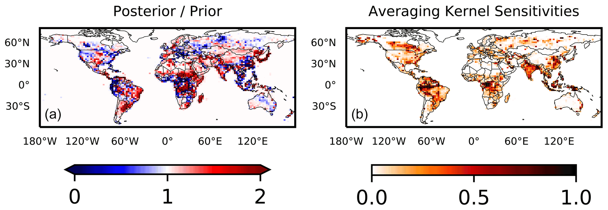
Figure 2 (a) Corrections to prior estimates of methane emissions on the 2^∘ × 2.5^∘ grid and corresponding averaging kernel sensitivities. (b) The averaging kernel sensitivities are the diagonal elements of the averaging kernel matrix for the inversion. The trace of the averaging kernel matrix defines the degrees of freedom for signal (DOFS) for the inversion, shown in the inset.

Assuming that the problem for quantifying methane fluxes from observed concentrations is linear, or only moderately nonlinear, then the fluxes, $\widehat{x}$, can be related to observed methane concentrations using the following equation (Rodgers, 2000):

$$\begin{array}{}\text{(2)}& \widehat{\mathit{x}}={\mathit{x}}_{\mathrm{A}}+\widehat{\mathbf{S}}{\mathbf{K}}^T{\mathbf{S}}_y^{-\mathrm{1}}\left(\mathit{y}-\mathbf{K}{\mathit{x}}_{\mathrm{A}}\right).\end{array}$$

The posterior error covariance matrix $\widehat{\mathbf{S}}$ is given by

$$\begin{array}{}\text{(3)}& \widehat{\mathbf{S}}=({\mathbf{K}}^T{\mathbf{S}}_y^{-\mathrm{1}}\mathbf{K}+{\mathbf{S}}_{\mathrm{A}}^{-\mathrm{1}}{)}^{-\mathrm{1}}.\end{array}$$

This top-down flux inversion also provides the spatial resolution matrix or averaging kernel matrix A, which defines the sensitivity of the solution to the true state:

$$\begin{array}{}\text{(4)}& \mathbf{A}=\mathbf{I}-\widehat{\mathbf{S}}{\mathbf{S}}_{\mathrm{A}}^{-\mathrm{1}}.\end{array}$$

Summing the diagonal elements of the averaging kernel for a given region provides the degrees of freedom for signal (or DOFS), a useful metric for the sensitivity of the observing system to the underlying fluxes as it describes the sensitivity of the estimated fluxes to the actual distribution of fluxes (Rodgers, 2000). Figure 2b shows the averaging kernel sensitivities (or diagonal elements of the averaging kernel matrix) of the inversions. The averaging kernel sensitivities are highest over major anthropogenic source regions, where the methane emissions are largest and the observations have a good ability to determine the posterior solution independently of the prior estimate. The inversion has ∼ 402 DOFS for methane emissions, meaning that it contains 402 independent pieces of information on the distribution of methane emissions. Although our flux inversion is based on the top-down setup described in Qu et al. (2021), this value is larger than the DOFS reported in Qu et al. (2021) because that estimate separates wetlands from non-wetlands in the inversion scheme, whereas the flux estimate used here does not. The posterior/prior ratios for the 2019 inversion in Fig. 2a show consistent upward adjustments in the southern–central US, Venezuela, and the Middle East and downward adjustments in the western US and North China Plain, consistent with Qu et al. (2021) and Zhang et al. (2021).

If the matrix S_A in Eqs. (1) and (3) represents the actual a priori uncertainty corresponding to the a priori x_A, then the posterior error covariance describes the total error for the estimate (Rodgers, 2000). In practice, the matrix S_A represents a “constraint matrix” that is either a best guess for uncertainties of fluxes (e.g., assumed here to be 50 %) within a grid and/or is constructed to ensure the inversion converges, typically because systematic errors in the data and/or the model or numerical instabilities make it challenging to find a global minimum in the cost function as shown in Eq. (1) (Bowman et al., 2006). In the case where S_A represents a constraint matrix, the total posterior error becomes

$$\begin{array}{}\text{(5)}& {\mathbf{S}}_{\mathrm{tot}}=\left(\mathbf{I}-\mathbf{A}\right){\mathbf{S}}_{\mathrm{A}}^{\mathrm{true}}(\mathbf{I}-\mathbf{A}{)}^{\mathrm{T}}+\widehat{\mathbf{S}}{\mathbf{K}}^{\mathrm{T}}{\mathbf{S}}_y^{-\mathrm{1}}\mathbf{K}\widehat{\mathbf{S}},\end{array}$$

where ${\mathbf{S}}_{\mathrm{A}}^{\mathrm{true}}$ is the a priori uncertainties for the estimate. In practice, ${\mathbf{S}}_{\mathrm{A}}^{\mathrm{true}}$ can be challenging to calculate due to lack of information about the emissions or fluxes and may not even be invertible because of correlations within the matrix. However, we use a set of informed inventories and models to generate a prior covariance for methane emissions as described in the next section. As discussed in Worden et al. (2004), the smoothing error in the estimate is the first term on the right-hand side, and the error due to measurement uncertainty is the second/middle term. While the variables in Eq. (5) are representative here of the top-down flux estimate, the formulation can be generalized for any estimate to support interpretation of the results. For example, in a system with perfect resolution the averaging kernel matrix becomes the identity matrix and the smoothing error becomes 0, hence the reason that improving the spatial resolution reduces the smoothing error, an important goal which can be realized with the increased observation density of upcoming satellites such as CO2M, Methane-Sat, and Carbon Mapper. Equation (5) also demonstrates that poorly characterized prior uncertainties in one region affect an estimate in another regions because of cross-terms in the averaging kernel matrix A. This aspect of top-down inversions must therefore be accounted for when interpreting the seasonality and magnitude of top-down fluxes (e.g., Ma et al., 2021).

Systematic errors can be included by adding the following term: $\widehat{\mathbf{S}}{\mathbf{K}}_{\mathrm{sys}}^{\mathrm{T}}{\mathbf{S}}_{\mathrm{sys}}^{-\mathrm{1}}{\mathbf{K}}_{\mathrm{sys}}^{\mathrm{T}}\widehat{\mathbf{S}}$, where K_sys is the Jacobian that describes the sensitivity of the modeled concentrations to different parameters in the model that relate emissions to concentrations and S_sys is a matrix containing uncertainties for the model or data parameters. In this paper we do not explicitly calculate systematic errors for the fluxes. We are currently studying how to empirically evaluate systematic errors in the flux estimate, following the approach in Jiang et al. (2015) for use in quantifying uncertainties in methane fluxes and emissions.

Evaluation of top-down flux estimates

The combination of model (GEOS-Chem) and data (GOSAT) used to quantify methane fluxes has been evaluated previously by comparing prior and posterior model concentrations to independent data. Maasakkers et al. (2019) find that posterior methane concentrations have correlations (R²) of 0.76, 0.81, and 0.91 with data from surface sites, aircraft, and total column data, respectively. These correlations are essentially the same as those for the GEOS-Chem prior concentrations, likely because these measurements are taken in background regions away from sources. These comparisons between posterior concentrations with independent datasets demonstrate that the GEOS-Chem model with GOSAT data has skill in quantifying atmospheric methane concentrations and that assimilating GOSAT data into GEOS-Chem for the purpose of quantifying fluxes is at least as skillful as using prior information when looking at background regions away from emissions sources. Changes in fluxes based on GOSAT data are therefore driven entirely by differences in satellite-observed concentrations over source regions.

2.2 Projecting fluxes to emissions and their uncertainties

The derivation that describes how to project top-down fluxes back to emissions by sector at arbitrary resolution is described in Cusworth et al. (2021b) and summarized in this section.

For policy relevance and CH₄ budget quantification, we wish to optimize emissions (z) using atmospheric observations; i.e., we want to compute the explicit posterior representation without re-simulation of an atmospheric transport model. The relationship we use between emissions z and fluxes x is simple aggregation (the total flux within a grid box is the sum of emissions) and can be represented by matrix M:

$$\begin{array}{}\text{(6)}& \mathit{x}=\mathbf{M}\mathit{z}.\end{array}$$

The solution for projecting fluxes back to emissions takes the form (Cusworth et al., 2021b)

$$\begin{array}{}\text{(7)}& \begin{array}{rl}\widehat{\mathit{z}}& ={\mathit{z}}_{\mathrm{A}}+\widehat{\mathbf{Z}}{\mathbf{M}}^T{\widehat{\mathbf{S}}}^{-\mathrm{1}}\\ & \left[\left(\mathbf{I}-\widehat{\mathbf{S}}{\mathbf{S}}_{\mathrm{A}}^{-\mathrm{1}}\right)({\mathit{x}}_{\mathrm{A}}-\mathbf{M}{\mathit{z}}_{\mathrm{A}})+\left(\widehat{\mathit{x}}-{\mathit{x}}_{\mathrm{A}}\right)\right],\end{array}\end{array}$$

where $\widehat{\mathit{z}}$ is the posterior emissions vector with error covariance ($\widehat{\mathbf{Z}}$) and I is the identity matrix. The posterior emission error covariance matrix $\widehat{\mathbf{Z}}$ is calculated explicitly given M, S_A, $\widehat{\mathbf{S}}$, and the prior emissions error covariance matrix Z_A:

$$\begin{array}{}\text{(8)}& \begin{array}{rl}\widehat{\mathbf{Z}}& ={\left({\mathbf{M}}^T\left({\widehat{\mathbf{S}}}^{-\mathrm{1}}-{\mathbf{S}}_{\mathrm{A}}^{-\mathrm{1}}\right)\mathbf{M}+{\mathbf{Z}}_{\mathrm{A}}^{-\mathrm{1}}\right)}^{-\mathrm{1}}\\ & ={\left({\mathbf{M}}^T\left({\mathbf{K}}^T{\mathbf{S}}_{\mathit{y}}^{-\mathrm{1}}\mathbf{K}\right)\mathbf{M}+{\mathbf{Z}}_{\mathrm{A}}^{-\mathrm{1}}\right)}^{-\mathrm{1}}.\end{array}\end{array}$$

This solution depends on the top-down flux inversion providing the inversion characterization products (i.e., the flux prior x_A and flux constraint matrix S_A and the flux Hessian $\widehat{\mathbf{S}}$). Note that here we must use the Hessian as described in Eq. (3), not the total posterior covariance as described in Eq. (5) (Cusworth et al., 2021b). To quantify the set of sectoral emissions $\widehat{z}$, corresponding prior emissions z_A and covariance matrix Z_A must be provided on the desired spatial grid; in this study we choose a 1^∘ long–lat grid. Note that the emissions and their prior uncertainties used to generate prior fluxes for the top-down flux inversion (x_A) can be different from those used to project the top-down fluxes back to sectoral emissions for linear or moderately nonlinear problems (e.g., Rodgers and Connor, 2003; Bowman et al., 2006), as the information from the measurement is preserved in the ${\mathbf{K}}^T{\mathbf{S}}_{\mathit{y}}^{-\mathrm{1}}\mathbf{K}$ term which is contained in ${\widehat{\mathbf{S}}}^{-\mathrm{1}}-{\mathbf{S}}_{\mathrm{A}}^{-\mathrm{1}}$ as shown in Eq. (8). This means that Mz_A can be different from x_A and their corresponding covariances, as long as the inversion problem is linear or only moderately nonlinear (Bowman et al., 2006; Cusworth et al., 2021b). However, the interpretation of fluxes will be different if these matrices (S_A and Z_A) are inconsistent (e.g., Shen et al., 2021), that is, S_A≠MZ_AM^T.

The uncertainty for any given element of the state vector z is generally given by the square root of the diagonal element of the total error covariance and includes the effects of the limited spatial resolution of the top-down flux and how this projects uncertainties from one grid box and sector into another grid box and sector, as discussed in the previous section. For example, the estimate for the emissions for some emissions sector “i” at some long–lat grid box “j” is given by (Rodgers and Connor, 2003; Worden et al., 2004)

$$\begin{array}{}\text{(9)}& \begin{array}{rl}{\widehat{z}}_{ij}& =z_a^{ij}+A_{ij,ij}\left(z_{ij}-z_a^{ij}\right)\\ & +\sum _{x,y}{A}_{ij,xy}\left({\mathit{z}}_{\mathrm{xy}}-{\mathit{z}}_{\mathrm{a}}^{xy}\right)+{\mathit{\delta }}_{ij},\end{array}\end{array}$$

where the italicized variables in Eq. (9) are scalar representations of the variables in Eqs. (7) and (8), the index “x” represents all sectors, the index “y” represents all other lat–long elements, and matrices and vectors are boldfaced. Note that the paired indices x and y exclude the paired indices i and j. The variable “z_xy” represents the “true” value corresponding to the estimate “${\widehat{z}}_{ij}$”, and the variable δ_ij represents the error due to random noise (we exclude systematic error here to simplify the math, but Eq. (9) can be expanded to include this term). Of course we do not actually know the true value and its errors, but Eq. (9) allows us to represent them in a manner than allows us to calculate their statistics. The total error for ${\widehat{z}}_{ij}$, equivalent to an element of the total error in Eq. (8), is

$$\begin{array}{}\text{(10)}& \begin{array}{rl}E\left|\left|{\widehat{z}}_{ij}-z_{xy}\right|\right|& =\left(\mathrm{1}-A_{ij}\right)Z_a^{ij}(\mathrm{1}-A_{ij}{)}^T\\ & +\sum _{x,y}{A}_{ij,xy}{Z}_a^{xy}{A}_{ij,xy}^{\mathrm{T}}+S_{ij}^n,\end{array}\end{array}$$

where the $E\left|\right|\left|\right|$ term describes the expectation operator for calculating the statistics of the quantity of interest (Bowman et al., 2006). The diagonal elements of the total error covariance therefore include the effect of the limited spatial resolution through the second term on the right-hand side of Eq. (10), which projects prior uncertainties from one region and sector (x,y) into the region and sector of interest (i,j). The last term is the covariance due to measurement noise. As the spatial resolution increases, the averaging kernel matrix converges towards the identity matrix; in this limit the first and second terms on the right-hand side converge to 0 such that the total error is due to noise (last term in Eq. 10) and any residual systematic errors (not shown in Eq. 10 but discussed in the previous section). Improving the spatial resolution of the methane emissions estimate therefore improves the accuracy.

In order to calculate the uncertainty for an aggregation of the elements of the state vector z (e.g., the coal sector for a country), instead of an individual element, we must sum the desired set of elements [z_M,n], where the index “M” represents the sector (e.g. coal), and the index “n” represents all latitude and longitudes that make up a country. The uncertainty (squared) for this term is then:

$$\begin{array}{}\text{(11)}& {\mathit{\sigma }}_{M,N}^{\mathrm{2}}={\mathit{h}}_n{\widehat{\mathbf{Z}}}_{Mn}{\mathit{h}}_n^T,\end{array}$$

where h_n is a vector that is the same length as [z_Mn], with values of one in each element and ${\widehat{\mathbf{Z}}}_{Mn}$ is the square sub-matrix of the covariance matrix Z corresponding to [z_mn] (e.g. the country and emission sector of interest). The subscript is summed over all lat/lons “n” for country “N”.

2.3 Generation of prior emissions, covariances, and uncertainties

In order to project fluxes from a top-down inversion back to emissions using the approach described in Sect. 2.2, sectoral emissions and their covariances, or z_A and Z_A, at the desired spatial resolution are required. One challenge with the flux to emissions projection is that the a priori covariance matrix Z_A must be inverted (Eq. 8), which can be computationally expensive because this matrix can be quite large because the number of sectors and spatial resolution of the emissions increase and because correlations within the matrix (next section) make it challenging to invert. In order to reduce computational expense for our chosen spatial resolution of 1^∘ resolution (prior to calculating country-wide emissions), we disaggregate global emissions into eight regions (Table 2) chosen by regions with peaks in the inversion sensitivity to the underlying fluxes as shown by the averaging kernel diagonals in Fig. 2. The different categories are shown in Table 2 for each region and by sector along with the provenance (or paper reference) in the second column. Cross-terms in the averaging kernel (Eqs. 5, 9, and 10) matrix demonstrate that the change in emissions in one region affect the estimated emissions in another. Subdividing the fluxes into these eight regions therefore introduces an extra error term in the total error covariance for each region; however, this extra error is automatically included in the total error covariance for each region as demonstrated by Eq. (10).

Table 2 Prior emissions by source and regions. Single values for uncertainties are calculated by projecting the corresponding covariance to a single number for the indicated long–lat region and taking the square root. Total values show a range of uncertainty, with the lower bound being the sum (squared) of the individual region or sector (assumes errors are uncorrelated) and the upper bound being the sum of the errors (assumes errors are completely correlated). The following references indicate the source for each emission type: (1) NASA CMS V1.0 (Wolf et al., 2017), (2) EDGAR 6.0 (Crippa et al., 2020), (3) NASA GFEI V1 (Scarpelli et al., 2020), (4) GFED 4.1 (van der Werf et al., 2017), (5) WETCHARTS 1.3.1 (Bloom et al., 2017), (6) GCP (Poulter et al., 2017), and (7) Etiope et al. (2019). The target uncertainty for each region and sector is given in parentheses underneath each region.

Our prior emission distribution and magnitude represent, by necessity, a set of ad hoc choices that are informed by the scientific literature and experience of the co-authors of this paper in developing top-down flux estimates. For example, our chosen resolution for reporting sectoral emissions is 1^∘, which represents a compromise between computational expense while minimizing representation errors when quantifying emissions for each country, which in turn is needed for these estimates to inform the global stock take. Future research will evaluate whether higher-resolution emissions estimates by sector can be quantified given the computational expense of inverting Eq. (8); our motivation for reporting top-down estimates at a higher resolution is because many of the inventories are at these scales (e.g., 0.1^∘) and also to better utilize high-resolution emissions estimates now available by aircraft data (e.g., Duren et al., 2019) and from upcoming satellites such as Carbon Mapper (e.g., Cusworth et al., 2019; 2021a).

We make the following choices for which sectoral emission type is represented: wastewater is not explicitly estimated, as these emissions are spatially correlated with landfill emissions based on inspection of EDGAR inventories when projected to 1^∘ resolution. The waste category should therefore be interpreted as a combination of landfill and wastewater. We also did not consider biofuels or termites for this estimate as they represent a small component of the budget. For these reasons, the biofuel and termite components of the methane budget will slightly bias our other sectoral estimates by 15–30 Tg CH₄ yr⁻¹ based on bottom-up estimates reported in Saunois et al. (2020). On the other hand, emissions for seeps are included, as bottom-up inventories suggest these could be as large as 30 Tg CH₄ yr⁻¹; however, given the co-location of seep emissions with oil and coal (Fig. 3), care must be taken in interpreting our results for seep emissions estimates. Our prior emissions for livestock are from a NASA Carbon Monitoring System product (Wolf et al., 2017) and are found from post-processing to be too low by ∼ 25 % due to not including a scaling factor in the overall emissions. Nonetheless, we keep the current set of (low) prior livestock emissions of ∼ 89 Tg CH₄ yr⁻¹ as they demonstrate (along with the analysis in Sect. 3.3, Fig. 6) that our total results are largely independent of the choice of priors because of the sensitivity of the fluxes to the underlying emissions as shown in Fig. 2b. A future version of these estimates will have an updated prior for livestock emissions and will include termites, wastewater, and biofuels. Although there can be many emissions within a single grid box, uncertainty can still decrease for each emission type as shown in Eq. (8), which shows that these correlations are quantified in the posterior covariance.

Uncertainty reduction of a particular emission therefore depends on the magnitude of the emission and its uncertainty, its correlations with nearby emissions of the same type (next section), and the magnitude and uncertainty of emissions within the same grid box.

Prior wetland emissions are based on an ensemble of process models from the WETCHARTS system and the Global Carbon Project (Bloom et al., 2017; Poulter et al., 2017; Ma et al., 2021) and include the effects of lakes and rivers. A future version of this system will separately estimate these other sectors of the methane budget if further analysis using other satellite data (e.g., TROPOMI) shows that they can be distinguished from these other sectors.

2.3.1 Covariance generation

Generating representative prior covariances is challenging as there are few global studies that allow for accurate representation of uncertainties for emissions across the globe and their correlations that are based on data and/or well-calibrated models. This problem exists not just for methane emissions, but also for other inverse problems where there are few data representative of the quantities of interest (e.g., with remote sensing; Worden et al., 2004). For this reason we need to make another set of ad hoc choices that is based on prior research in order to generate the covariances for each sector. We therefore use the following approach: first we assume that the total anthropogenic emissions (by sector) in Annex 1 countries have an uncertainty of 15 %. For example, we assume that the total error for the North American coal sector is ∼ 15 %, and so on for each anthropogenic sector. Similarly, the total error for Annex 2 regions is 30 %. These targeted uncertainties are listed underneath the label for each region in Table 2. These uncertainties are reported in Janssens-Maenhout et al. (2019) and are based on “expert opinion”, as quantifying uncertainties over a country or region using bottom-up approaches can be challenging. Total regional uncertainty for a specific sector is calculated using Eq. (11). In order for sectoral emissions at 1^∘ resolution to project to a total regional uncertainty of 15 %, there must be significant uncertainty of any given emission within that 1^∘ grid cell. However, even assuming very large uncertainties for an emission within a 1^∘ grid cell (e.g., 100 %), the regional total uncertainty can be much smaller than 15 % once projected over a large enough number of grid cells if the emission errors are assumed to be uncorrelated. To address this issue, we also add correlations between nearby emissions; we start the diagonal values at 0.7 (squared) of the prior emissions, or 70 % uncertainty, and with a correlation of 0.7 between neighboring emissions of the same type that are within 400 km (or four grid cells). The diagonal values and correlations are then adjusted until the projected uncertainty reaches 15 % (for Annex 1) or 30 % (Annex 2). Final values typically range from 0.6 (squared) to 1.0 for the diagonal and from 0.7 to 0.9 for the off-diagonal values with variations in these numbers because of the different spatial distributions of the emissions. These numbers for the correlation and length scale are based on regional studies for North America, which also indicate that uncertainties for nearby emissions should be correlated (e.g., Maasakkers et al., 2016, 2019).

For wetlands, we use a slightly different approach for generating covariances. Here we calculate the root mean square (rms) of an ensemble of different wetland process models (Bloom et al., 2017; Poulter et al., 2017; Ma et al., 2021) for a given region. We then follow a similar covariance generation approach as used for the anthropogenic emissions, iterating with different diagonal and off-diagonal values until the projected uncertainty for a region is approximately the same as the corresponding variance of the models.

While generating representative prior covariances is challenging, Eqs. (7) and (8) from the previous section allow us to swap in better priors and prior covariances as these become available. For example, if a researcher finds that the uncertainties expressed in Z_A over a given region for a given sector should be 10 % instead of the value used (approximately 70 %), then it is straightforward to update the covariance matrix to reflect this improved knowledge so that the attribution to each sector is improved. Of course this improved information could also be used to improve the S_A constraint matrix in Eq. (1) to improve convergence of the top-down flux estimate. Furthermore, the updated posterior covariances can be used for the next flux inversion based on other independent data, and at some point these covariances, because they are based on observations, will best reflect our knowledge of the methane emission. Covariances and prior emissions are all publicly available, as well as python code that demonstrates how to use these files, so that a researcher can determine how other priors and changes to their uncertainty structure affect this top-down result or how to use them for their own top-down inversions. Links to these data and codes are in the Data Repository section (Sect. 5).

2.3.2 Uncertainty calculation approach

The uncertainties shown in Tables 1 and 2 are calculated in the following manner. First the prior uncertainties for each sector and for each region shown in Table 2 are calculated by projecting the regional (e.g., North America, South America) posterior error covariance to a single number corresponding to the mean emissions for that region using Eq. (11). One approach is to then assume that these uncertainties are independent of each other, in which case they are added in quadrature to get the total value; this is the smaller uncertainty shown in the Total column in Table 2. However, another method is to assume that the uncertainties are 100 % correlated, such that they should be added linearly; these are the values shown as the larger value in Table 2. We expect that the actual uncertainty is somewhere between these values. However, to be conservative, we only report the larger value in Table 1 and for the remainder of the paper.

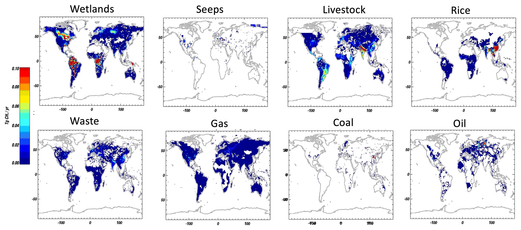
Figure 3 The square root of the diagonal of the a priori covariance for the eight largest sectors used in our analysis.

The prior uncertainties generated using the method described here are consistent with those reported in the literature even though the methodology differs. For example, the values shown in the “prior” column of Table 1 are consistent (within reported ranges or uncertainties) with the equivalent sectors discussed in Saunois et al. (2020) and with the regional EDGAR v4.3.2 inventories as discussed in Janssens-Maaenhout et al. (2019). A caveat is that Janssens-Maaenhout et al. (2019) also report global totals for each sector, from a range of inventories and models, that are 2–3 times larger for each sector than those shown here. Another caveat is that Saunois et al. (2020) include a freshwater category with a 120 ± 60 Tg CH₄ yr⁻¹ uncertainty, whereas this category is subsumed into our wetlands/aquatic sector.

Figure 3 shows the (square-root) diagonal of the covariance for each sector; as discussed previously, these are generally correlated with the magnitude of the emissions but also the chosen value for the regional total error (Table 2). Most of the sectors have enhancements and corresponding uncertainties that are spatially distinct. For example, the largest uncertainties for oil are located in eastern Europe and Russia, the largest uncertainties for coal are in China, and the largest uncertainties for gas are in North America and central Asia. In turn, these fossil emissions are spatially distinct from wetlands and livestock. However, the largest uncertainties for rice and waste can spatially overlap those of livestock, especially in India and Asia, which indicates that remote sensing will be challenged to distinguish these emissions.

3 Results

In this next section we first present global estimates, followed by a discussion of the sectoral emissions for the top 10 emitting countries and then emissions for all countries. Finally, we test whether different assumptions about bottom-up emissions as discussed in the recent literature, i.e., larger wetland/aquatic emissions (Rosentreter et al., 2021), and larger fossil emissions (Schwietzke et al., 2016) affect our conclusions about the top-down results presented here.

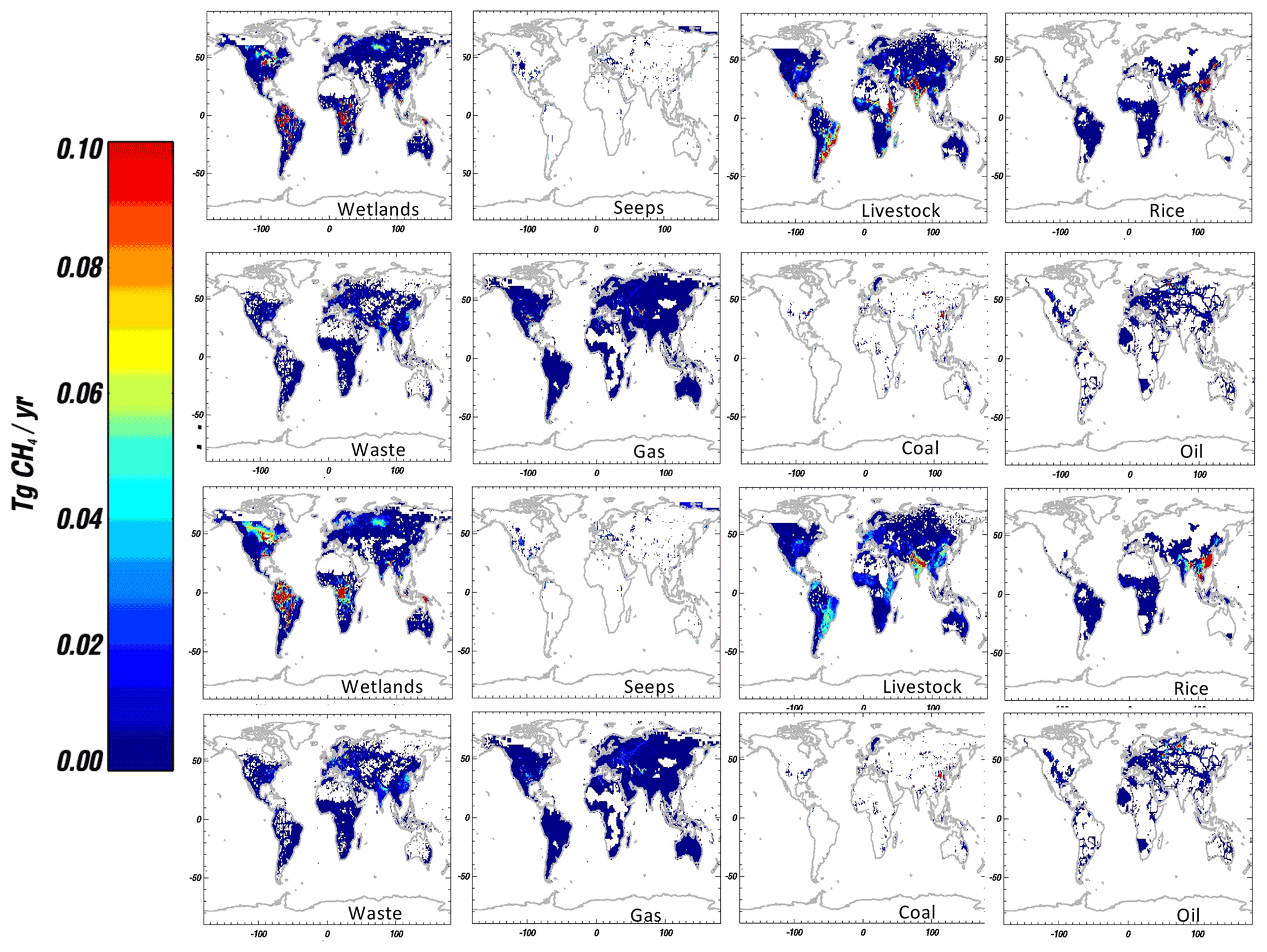
Figure 4 Top: posterior methane emissions. Bottom: posterior emissions uncertainty as calculated by the square root of the diagonal of the posterior covariance matrix.

3.1 Global methane budget by sector

Emissions by sector and their uncertainty at 1^∘ resolution are shown in Fig. 4, with the top set of panels showing the posterior emissions and the bottom set showing the uncertainties. As in Fig. 3, the uncertainty at each longitude–latitude grid element is given by the square root of the diagonal of the total error covariance. Uncertainty can decrease for emissions even when there is more than one type of emission in a grid box. As shown in Eq. (8), this uncertainty reduction depends on the magnitude of the emission and its uncertainty, its correlations with nearby emissions of the same type (Sect. 2.3), and the magnitude and uncertainty of emissions within the same grid box.

Inspection of Fig. 4 (bottom panel) and Fig. 3 shows that reduction of uncertainty in many parts of the world relates to the prior, such as the larger wetlands and agricultural regions in India and Asia. The right panel of Table 1 shows the global total posterior emissions by sector. The increase in sectoral emissions relative to the prior for the agriculture sector and reduction in fossil emissions reflect the top-down flux estimates (Fig. 2), which show a lower posterior flux relative to the prior in fossil-emitting regions such as Russia and North America (with the exception of the southern USA) and increases in regions where livestock and rice emissions are expected to be the largest source relative to other emissions such as in India, Brazil, Argentina, and eastern Africa.

3.1.1 Comparisons to previous top-down inversions using GOSAT and GEOS-Chem

Our results are consistent with previous top-down estimates based on the satellite GOSAT data. For example, the results here are based on the inversion framework from Zhang et al. (2021) and Qu et al. (2021) and are therefore generally consistent for the larger emissions such as wetlands and livestock or the emissions which are spatially distinct from other sources and therefore easier to resolve with remote sensing such as oil and coal. However, our estimates for rice, waste, and seeps are very different, and this is likely because our choices of priors for these sectors are different and because Qu et al. (2021) use a uniform scaling approach to project fluxes to emissions, whereas we account for the prior uncertainties. Similarly, our results for wetlands, livestock, and fossil emissions are consistent with previous GOSAT-based inversions (e.g., Maasakkers et al., 2019; Zhang et al., 2021), with the caveat that these estimates are for earlier time periods and changes in emissions can affect interpretation of any differences. Ma et al. (2021) use GOSAT-based wetland estimates to show that wetland emissions for the years 2010–2018 are likely even lower than our results. As with results presented here, they take into account the spatial resolution and prior of the top-down fluxes but use a different approach to quantify emissions; they select “high”-performing wetland models based on comparison of an ensemble of models with mean wetland emissions and temporal variability. The total emissions for these highest-performing models, 117–189 Tg CH₄ yr⁻¹, are lower but within the uncertainty of the results here. These differences in results, even when using similar models and data, highlight the importance of the choice of priors as well as the methodology by which fluxes are projected back to emissions, as estimates for sectoral emissions can be very different from one estimate to the other depending on these choices.

3.1.2 Comparisons to top-down inversions from GCP

Emissions in Table 4 can be compared to top-down inversions from the Global Carbon Project (GCP) when aggregated into combined categories (Saunois et al., 2020). For example, our agriculture and waste emissions are ∼ 263 ± 24 Tg CH₄ yr⁻¹, anthropogenic fossil emissions are 82 ± 12 Tg CH₄ yr⁻¹, and natural wetland/aquatic emissions are 180 ± 10 Tg CH₄ yr⁻¹. These are within the reported uncertainties of top-down inversions in GCP, which are [205–246 Tg CH₄ yr⁻¹], [91–121 Tg CH₄ yr⁻¹], and [155–217 Tg CH₄ yr⁻¹], respectively, but on the high side for agriculture and waste and on the low side for fossil emissions. These differences between GCP and emissions reported here likely represent the differences in information content and sampling from satellite versus ground-based data as most of the top-down ensembles reported in Saunois et al. (2020) are based on in situ measurements which are typically in background regions and which are therefore not as sensitive to the spatial distribution of emissions as the satellite-based estimates (e.g., Fig. 6 from Yin et al., 2021). However, one set of results included with the top-down GCP results that is based on GOSAT data (i.e., Tsuruta et al., 2017) is consistent with our results as they report biospheric emissions of ∼ 172 ± 29 Tg CH₄ yr⁻¹. Note that the other paper citations in the GCP methane paper that indicate use of GOSAT data describe the model setup and results for CO emissions or for regional results, so we cannot explicitly compare them to their results.

3.1.3 Fossil emissions

Our posterior results for anthropogenic fossil emissions (82 ± 12 Tg CH₄ yr⁻¹) and natural ones (22.5 ± 3.8) are lower than our prior ones and in general do not reflect recent papers that suggest much higher fossil emissions using measurements of δ¹³CH₄ (e.g., Schwietzke et al., 2016, indicates 211 ± 33 Tg CH₄ yr⁻¹ for anthropogenic + natural fossil emission) or measurements over USA basins upscaled from aircraft (e.g., Alvarez et al., 2018). However, as discussed in Turner et al. (2019), care must be taken in using isotope measurements to infer the partitioning of methane sources because of large uncertainties in the emissions factors of different sources at different latitudes. Upscaling can also have large uncertainties as emissions factors that relate activity data to emissions can vary significantly from region to region. Our global posterior fossil emissions are consistent with more recent reports of fossil emissions, ∼ 84 Tg CH₄ yr⁻¹, to the UNFCCC (Scarpelli et al., 2022) for 2019, suggesting that our lower posterior estimates of fossil emissions are not unreasonable.

Onshore geological seeps represent another largely uncertain source of fossil emissions, with values ranging from 2 to 30 Tg CH₄ yr⁻¹. For example, the top-down flux estimate, used as a basis for the sectoral emissions attribution, assumes a prior of ∼ 2 Tg CH₄ yr⁻¹. However, our choice of prior (part of the z_A vector, Eq. 7) is based on Etiope et al. (2019) with a value of 32.0 ± 6.2, resulting in a posterior of 22.5 ± 3.8 Tg CH₄ yr⁻¹. This reduction in uncertainty is substantial, suggesting that remote sensing is providing good information about this source. A caveat is that seep emissions tend to overlap those from coal and oil (Fig. 4), suggesting a potential equifinality between these emissions estimates. Combining fossil emissions from the seep category with anthropogenic fossil emissions increases the overall fossil total and would make the total fossil emissions (natural + anthropogenic) consistent with top-down results from GC. Based on these results, we suggest this category attention deserves measurements, especially from the upcoming high-resolution greenhouse gas measurements such as Carbon Mapper.

3.2 Top 10 emitting countries

Figure 5 lists the top 10 emitting countries ranked by total anthropogenic emissions as calculated using this remote sensing system. Sectoral attribution is based on the nine categories in Table A1; here we combine categories so that they are similar to what is being reported for the CO₂-based carbon inventories. The different categories are AF, which includes the sectors for agriculture (livestock and rice) and fires. This category is similar to the Agriculture, Forestry, and Land Use categories or “AFOLU” as used in CO₂-based carbon inventories. W is the waste category and FF is the fossil category, which includes extraction, transport, and use of coal, oil, and natural gas (Scarpelli et al., 2020, 2022). The Natural category includes wetlands and geological seeps. The top five emitting countries are essentially the same for bottom-up and top-down. However, top emitting countries have the most emissions from the agriculture sector, likely due to livestock (see Table A1). While top-down and inventory emissions for China, the USA, and Indonesia are consistent, there are major differences between our top-down results and inventories for the other countries. We next compare these results to those of previous studies; however, as stated earlier, these results should be treated cautiously and as a starting point for future research as differences can also be due to unquantified uncertainties in either the remote sensing data or the transport model used to relate concentrations to fluxes.

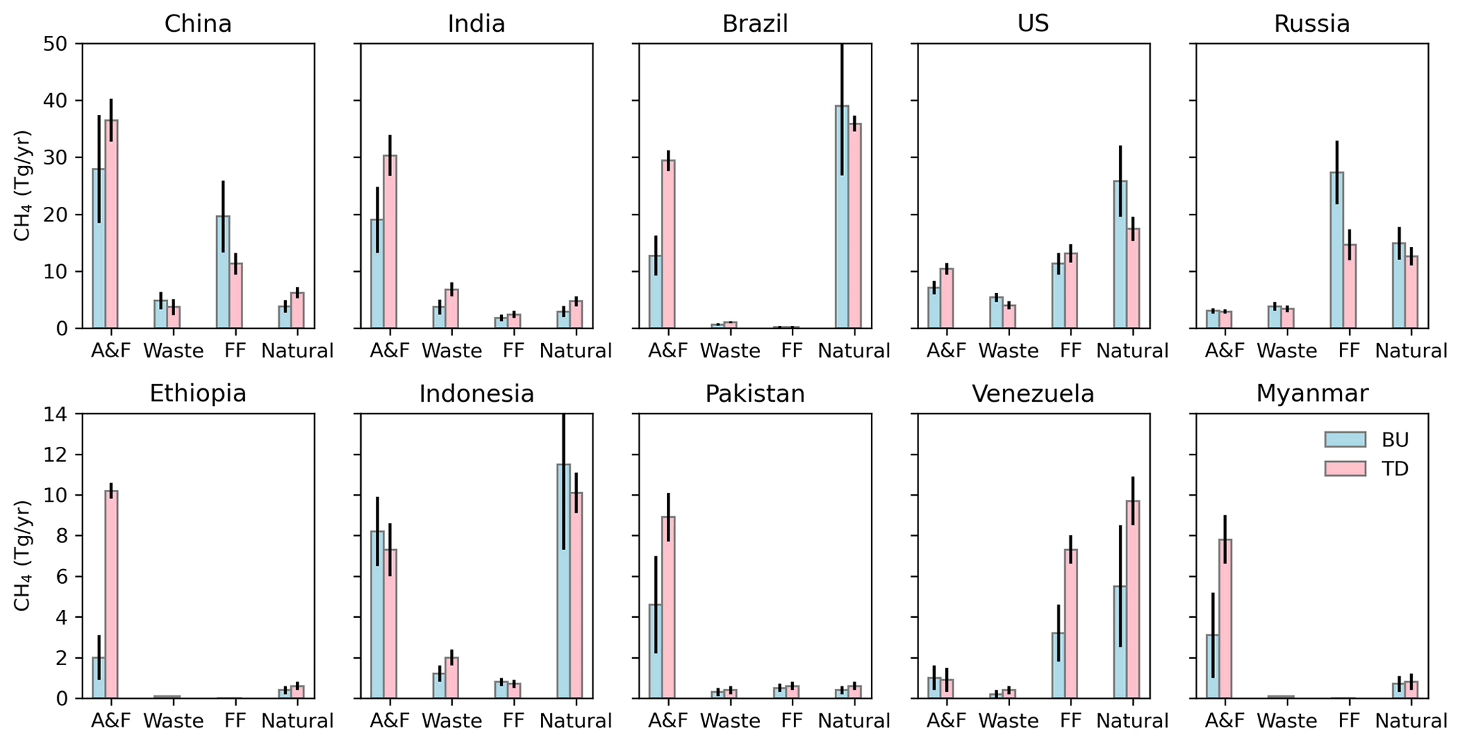
Figure 5 Emissions by sector for the top 10 emitters. AF represents agricultural and fires. FF represents fossil fuels or coal, oil, and gas. Natural represents wetlands, aquatic sources, and geological seeps. Bottom-up (BU) inventory estimates are shown as blue bars, and the remote sensing/top-down (TD) estimates are shown as pink bars. The uncertainties in both quantities are shown as black lines. Uncertainty calculations for bottom-up and top-down estimates are discussed in Sect. 2.

Our results are consistent with those from Maasakkers et al. (2019), Zhang et al. (2021), and Qu et al. (2021); however, this is not too surprising as emissions that are reported here are based on the flux inversion system from these studies. A notable difference in methodology is Qu et al. (2021), who also derive fluxes based on total column data from TROPOMI. However, Qu et al. (2021) find that country totals for the top five are essentially the same based on GOSAT and TROPOMI except for Brazil but attributed large differences between TROPOMI and GOSAT to systematic errors in the TROPOMI total column data related to low surface albedo over Brazil; consequently, the TROPOMI-based estimates in this region should be treated more cautiously.

Comparisons of these results to other estimates discussed in the literature can show substantial differences in either total emissions or attribution or both. For example, Ganesan et al. (2017), using in situ and satellite atmospheric methane data, find much lower total Indian emissions of 22 ± 2.3 Tg CH₄ yr⁻¹ for the 2010–2015 time period as compared to 39.5 ± 5.4 for our study (and the Qu et al., 2021 and Zhang et al., 2021 studies) and 36.5 ± 5.3 from Janardanan et al. (2020). Miller et al. (2019) provide similar total emissions for China of 61.5 ± 2.7 Tg CH₄ yr⁻¹ but different partitioning; for example, they find that coal is the largest source of emissions based on comparison of top-down fluxes to EDGAR emissions and using a relative weighting attribution flux to emissions attribution approach, whereas we find that agriculture (primarily rice, Table A1 in Sect. 4) is the largest sector. A major caveat is that attribution of emissions from total fluxes is challenging for China because many of the strongest emissions (e.g., coal, livestock, and rice as shown in Figs. 3 and 4) overlap within the spatial resolution of the top-down estimate, which is less than 2.5^∘ based on gridding used for the flux inversion and the variable sensitivity of the averaging kernel. While in principle these uncertainties due to limited spatial resolution are quantified based on our assumed prior covariance for each sector, it is quite possible that both our choice of the location of the emissions and corresponding prior covariance are incorrect due to less confidence in the emissions characterization in this region (Janssens-Maenhout et al., 2019). Our results are consistent (within uncertainties) for recent results by Deng et al. (2022); total anthropogenic emissions from Table A1 are within uncertainties of reported bottom-up and top-down total anthropogenic emissions shown in Fig. 4 of Deng et al. (2022), even if the attribution of emissions may differ. Similarly, top-down-based country-level anthropogenic emissions from Stavert et al. (2022) are consistent, when we are able to directly compare emissions country to emissions country, although many of their emissions only agree at the outer edge of the reported uncertainties.

We find that Myanmar has anonymously large agricultural emissions (primarily from livestock, Table A1, Sect. 4) relative to prior assumptions. Given that the DOFS reported for Mynamar is 2.7, we expect that the fluxes here are well resolved, such that it is possible that poorly characterized prior emissions drive this difference between prior and posterior. For example, Janardanan et al. (2020) also report similar top-down emissions of 6.1 ± 0.8 Tg using a higher-resolution satellite-based flux inversion. However, an alternative explanation could be that errors in model transport could project to larger-than-expected fluxes (Eq. 9) in this region, as Jiang et al. (2013) find that regions with substantial atmospheric convection can have large biases in top-down surface emissions estimates.

Ethiopia also has larger-than-expected agricultural emissions (livestock emissions) as compared to the prior. As with Mynamar, the prior emissions could be too low. For example, the number of cattle and other livestock, between 80 and 90 million in 2015 and growing (Bachewe et al., 2020, https://www.statista.com/, last access: 21 May 2022), is not that different in size than US livestock, ∼ 93 million in 2021 (https://www.statista.com/), suggesting that they could also have comparable livestock emissions. An alternative explanation for this discrepancy is very low prior emissions in neighboring Sudan despite possible large numbers of cattle in this region as well (https://knoema.com/, last access: 21 May 2022), suggesting that livestock inventories in the eastern African regions need to be re-examined.

Russian posterior fossil emissions are substantially lower than those initially reported in Scarpelli et al. (2020), which are based on reports to the UNFCC in 2017. However, more recent reporting to the UNFCC also suggests a much smaller bottom-up fossil estimate of ∼ 7 Tg CH₄ yr⁻¹ (Scarpelli et al., 2022). Table A1 (next section) indicates that remote sensing provides the best information about Russian oil and to some extent coal emissions as the reduction of uncertainty is largest for these sectors but has little change for gas emissions. Total emissions for oil and coal are 11.2 ± 1.9, indicating that total fossil emissions are likely larger than expected for the latest reports to the UNFCC but smaller than previous ones. As discussed previously, these top-down estimates should be treated cautiously and only as a starting point for future studies due to the limited sensitivity and potential uncertainties in both top-down and bottom-up.

3.3 Results for all countries

This section presents the complete table (Table A1, Appendix A) of emissions by sector and country. As discussed previously in Sect. 2.1, we project the sectoral emissions in each 1^∘ grid to each country using a country map to quantify the emissions and their uncertainties for each country. The table is ordered by DOFS, which is a metric of sensitivity for inversion problems. As discussed in Sect. 2.1, the DOFS is a metric for the sensitivity of the flux estimate. For example, a DOFS of 1 means that this remote sensing system (GOSAT plus GEOS-Chem) can generally resolve the countries' total emissions, assuming the sensitivity is evenly distributed across the country. More DOFS means that more emissions can be spatially resolved. However, even a DOFS of 0.5 means that half of the estimate is weighted by the measurement, with the estimate increasingly weighted by the a priori one as the DOFS approaches 0. For these reasons we report estimates for all countries, even if the DOFS are effectively 0, as information about the a priori inventories from the measurement might be useful even if not well informed by the satellite data. To distinguish these different levels of sensitivity, we color countries with corresponding DOFS greater than 1.0 as green, between 0.5 and 1.0 as yellow, and below 0.5 as red.

The DOFS are calculated from the averaging kernel matrix provided by the GEOS-Chem-based inversion (Sect. 2.1). To calculate the DOFS for a given country, we project the diagonal of the averaging kernel (Fig. 2) to 1^∘ resolution and then add up these values based on the 1^∘ country map used in this study. Note that the total DOFS between the reduced resolution flux inversion and the 1^∘ map is preserved. Table A1 indicates that the GOSAT-based top-down estimate can quantify total emissions (i.e., reduce uncertainty) for approximately 57 countries as the DOFS for the 57th country is more than 1 and less than 1 for the 58th country. As discussed previously, as DOFS approaches 0, there is less reduction in uncertainty using the top-down system discussed here. Furthermore, inspection of Table A1 shows that even countries where DOFS are between 1 and 2 show little reduction of uncertainty; this happens because of cross-terms in the sensitivity project uncertainty from one sector or region into another, as shown in Eq. (10).

The astute reader will notice negative emissions in some countries in Table A1. Negative emissions are a possible solution for inverse problems using linear updates, such as used here, even if they are not physically possible. Typically negative emissions occur when there are limited constraints on emissions in one region with large values in the state vector in a neighboring region; this is also known as “jack-knifing” in the inverse community. For example, livestock emissions for Peru are shown to be negative in Table A1, likely because Peru is near the Amazon basin, which has substantive wetland emissions, and the cross-correlations between these regions result in negative values in Peru livestock. In this case we would assume there is no information from this remote sensing system on this category and ignore these results.

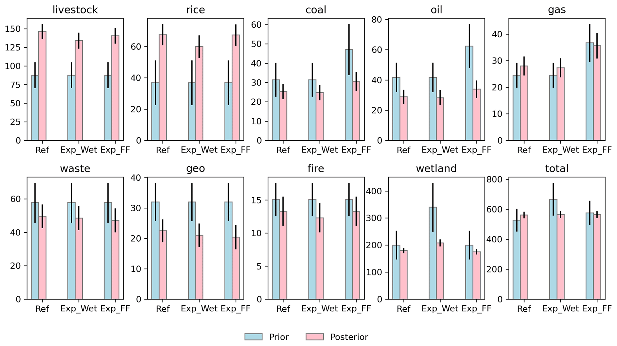
Figure 6 Comparison of total posterior emissions for the reference case (“Ref”, also Table 1 posterior) if prior wetland emissions are inflated (Exp_Wet) and if prior anthropogenic fossil emissions are inflated (Exp_FF).

3.4 What happens to the (top-down) methane budget if priors for wetland/aquatic and fossil emissions are substantially increased?

Equations (7) and (8) also allow us to test other prior emission inventories to determine whether they are consistent with top-down fluxes. This approach is similar to the “prior swapping” approach described in Rodgers and Connor (2003) but can also include “prior covariance swapping” as discussed in Cusworth et al. (2021b). This approach involves replacing the z_A and Z_A shown in Sect. 2.2 with different formulations. In this section we test what happens if we inflate the prior emissions for the wetland or fossil fuel categories such that they are consistent with other studies indicating much higher values than expected from top-down estimates, e.g., Rosentreter et al. (2021) for wetland/aquatic emissions and Schwietzke et al. (2016) for fossil emissions. Figure 6 shows the results of these two studies. The bars labeled “Ref” indicate the prior used for the results reported in this paper. The bars labeled “Wet” indicated the increased wetland study (which also includes increases to lake and river emissions as the wetland models include these categories, Bloom et al., 2017), and the bars labeled “FF” indicate the study where anthropogenic fossil fuels are increased by 50 %. We find that, even with very large prior emissions for wetland/aquatic sources, the posterior gives an estimate of 208 ± 12.8 Tg CH₄ yr⁻¹ as compared to 179.8 ± 10 for the reference values. This decrease from the inflated prior of ∼ 340 to 208 Tg CH₄ yr⁻¹ happens because the global total is constrained to ∼ 560 Tg CH₄ yr⁻¹ through knowledge of the methane sink and because wetland emissions tend to be spatially distinct from other sources.

For the same reasons, fossil emissions, especially coal, oil, and geological seeps, show a substantial decrease in uncertainty. Consequently, the posterior emissions differences between the reference and inflated fossil studies are consistent within uncertainty, and generally these emissions are much less than either the reference or inflated priors. For these reasons, it is challenging to reconcile these inflated aquatic emissions or inflated fossil emissions with top-down results. As noted previously, these comparisons should still be treated cautiously and as a starting point for further research because of poorly characterized systematic errors in the chemistry transport model used to relate observed concentrations to fluxes and because sources that are not included in the prior state vector but co-located with other sectors cannot be distinguished. For example, if there are significant (unspecified) aquatic emissions that are co-located with livestock emissions, then the corresponding livestock emissions estimate would be biased high.

4 Summary and future directions

In this paper we demonstrate, using a new Bayesian algorithm, estimates of emissions by sector at 1^∘ resolution and by country by using a combination of prior information of the emissions, satellite data, and a global chemistry transport model. Uncertainties are provided for representation (or smoothing) error and data precision but not for systematic errors in the transport model or data. Using a metric called the degrees of freedom for signal (DOFS), we show that the combination of GOSAT-based satellite data with the GEOS-Chem model and prior uncertainties can estimate total emissions for about 57 of the 242 countries, with only partial information for the remaining countries. Our results can be used for comparison to country-level, bottom-up inventories by sector that might be, for example, provided by the global stock take. However, any discrepancies between these top-down and inventory-based estimates should be considered a starting point for future investigations given the potential for systematic errors affecting the top-down results such as from accuracy limitations in the data or in the chemistry transport model used to estimate fluxes from the data (e.g., Buchwitz et al., 2015; Jiang et al., 2015; McNorton et al., 2020; Schuh et al., 2019). Alternatively, countries with little capability for quantifying bottom-up emissions could use these results, along with other published top-down estimates (e.g., Deng et al., 2021; Stavert et al., 2022), for their contribution to the global stock take.

In the absence of systematic errors, we find robust estimates for livestock, coal, oil, seeps, fires, and wetlands, as these can (on average) be distinguished from other sources using remote sensing given their distinct locations. Our results are consistent (within uncertainty) with previous top-down estimates such as the 2017 Global Carbon Project that are primarily based on in situ data. However, these remote sensing estimates are on the high side for agricultural and waste emissions and the low side for fossil and wetland emissions. On the other hand, total fossil emissions reported here are consistent with recent reports of fossil emissions to the UNFCCC (Scarpelli et al., 2022).

The new Bayesian algorithm we demonstrate can be used to test whether different prior emissions are consistent with our posterior emissions estimates. For example, we find that inflating the priors for wetland/aquatic fluxes or alternatively fossil emissions does not fundamentally alter our estimates for these sectors. Consequently, the remote sensing estimates reported here show much lower wetland and fossil emissions than these studies based on bottom-up models and isotope data and much larger agricultural and waste emissions. The largest differences between remote sensing and these other estimates occur in Brazil and India (primarily related to livestock), Russia (fossil emissions), and central and eastern Africa (livestock). These contrasting differences between the remote-sensing-based results and bottom-up models suggest that additional research is needed in these geographical areas to reconcile global methane budget estimates.

Future directions

We are evaluating how to characterize systematic errors related to the atmospheric chemistry transport model (e.g., Schuh et al., 2019) and in the satellite data to our error analysis, and we expect the next version of these estimates to contain these uncertainties. We also expect to add isotopic information through new flux estimates based on the surface network and the GEOS-Chem model; these independent data can be used to test the partitioning of biogenic, fossil, and pyrogenic emissions (e.g., Worden et al., 2017). We are also examining how to combine high-resolution emissions estimates based on aircraft data and imaging spectrometers such as GHG-Sat or Carbon Mapper with the top-down fluxes to improve inventory estimates at finer spatial scales than reported here. Finally, the posterior emissions and covariances demonstrated in this paper can be used as priors in subsequent emissions estimates using data from other measurements such as from the upcoming CO2M, Methane-Sat, and Carbon Mapper instruments.

Appendix A: Appendix table of emissions for each country ordered by DOFS

Table A1 Table of emissions for each country. This table provides the top-down and bottom-up estimates for each sector based on the methodology described in this paper. The table is ordered by DOFS, which is the metric for sensitivity for the remote sensing system described in this paper. The first row for each country provides the top-down result, and the second row is the bottom-up result. Prior inventories are shown in Table 2. Bold text is for results where DOFS > 1. Italicized text corresponds to 0.5 < DOFS < 1. Plain text corresponds to DOFS < 0.5.