An ensemble-variational inversion system for the estimation of ammonia emissions using CrIS satellite ammonia retrievals

An ensemble-variational inversion system is developed for the estimation of ammonia emissions using ammonia retrievals from the Cross-track Infrared Sounder (CrIS) for use in the Global Environmental Multiscale – Modelling Air quality and Chemistry (GEM-MACH) chemical weather model. A novel hybrid method to compare logarithmic retrieval parameters to model profiles is presented. Inversions for the monthly mean ammonia emissions over North America were performed for May to August 2016. Inversions using the hybrid comparison method increased ammonia emissions at most locations within the model domain, with total monthly mean emissions increasing by 11 %–41 %. The use of these revised emissions in GEM-MACH reduced biases with surface ammonia observations by as much as 25 %. The revised ammonia emissions also improved the forecasts of total (fine + coarse) ammonium and nitrate, as well as ammonium wet deposition, with biases decreasing by as much as 13 %, but they did not improve the forecasts of just the fine components of ammonium and nitrate. A comparison of biases resulting from inversions using different comparison methods shows favourable results for the hybrid comparison method.

1 Introduction

Ammonia (NH₃) is one of the most abundant reactive nitrogen species in the atmosphere. Major sources of ammonia include emissions from fertilizers, livestock, and biomass burning (Behera et al., 2013). Excess deposition of ammonia has been associated with eutrophication and soil acidification (Fangmeier et al., 1994; Krupa, 2003). As the primary basic gas in the atmosphere, ammonia plays a central role in the neutralization of acids and the formation of particulate matter (PM) in the atmosphere (Tsimpidi et al., 2007; Makar et al., 2009). And while ammonia has a relatively short atmospheric lifetime, on the order of hours to days (Van Damme et al., 2018), fine particulate matter can last much longer in the atmosphere, on the order of days to weeks (Seinfeld and Pandis, 2006). Particulate matter with diameters smaller than 2.5 µm (PM_2.5) has been associated with cardiovascular and respiratory disease and premature mortality (Pope et al., 2002; Burnett et al., 2014; Lelieveld et al., 2015). Additionally, inorganic aerosols can affect climate directly through radiative forcing (Adams et al., 2001; Martin et al., 2004) and indirectly through its effect on cloud formation (Abbatt et al., 2006). In contrast to trends of nitrogen oxides (NO_x) and sulfur dioxide (SO₂) that have declined over the last few decades in many regions, ammonia levels have either been constant or increasing in many parts of the world (Butler et al., 2016; Yao and Zhang, 2016; Warner et al., 2017; Van Damme et al., 2021).

Until recently, atmospheric ammonia observations were mainly limited to networks of ground-based measurements. The relatively short atmospheric lifetime of ammonia and the inhomogeneity of its sources result in a largely inhomogeneous distribution within the atmosphere. Accordingly, the limited spatial and temporal coverage of observations from these ground-based networks limits their ability to constrain ammonia emissions. While bottom-up emissions inventories can provide emissions estimates at a high spatial resolution, they generally rely on a variety of land-use specifications (such as farming practices) and emission factors that can be highly uncertain at the spatial and temporal scales required for modern chemical transport models. Due to these factors, large uncertainties in the spatial and temporal distribution of ammonia emissions exist in current inventories (Clarisse et al., 2009; Heald et al., 2012; Walker et al., 2012).

More recently, the development of retrieval algorithms for atmospheric ammonia used with satellite-borne instruments such as the Tropospheric Emission Spectrometer (TES) (Shephard et al., 2011, 2015), the Infrared Atmospheric Sounding Interferometer (IASI) (Clarisse et al., 2009; Van Damme et al., 2014), the Atmospheric Infrared Sounder (AIRS) (Warner et al., 2016), and the Cross-track Infrared Sounder (CrIS) (Shephard and Cady-Pereira, 2015; Shephard et al., 2020) has led to a wealth of new information on atmospheric ammonia. The wide spatial and temporal coverage of these observations has greatly improved our understanding of ammonia's global distribution (Clarisse et al., 2009; Shephard et al., 2011; Van Damme et al., 2014; Warner et al., 2016), seasonal variation (Shephard et al., 2011; Van Damme et al., 2014; Warner et al., 2016), long-term trends (Warner et al., 2017), presence in fire plumes (Coheur et al., 2009; Adams et al., 2019), large emissions point sources (Van Damme et al., 2018; Dammers et al., 2019), and dry deposition fluxes (Kharol et al., 2018).

The information contained within observational data can be blended with bottom-up emission inventories using inversion methods. Previous works, such as Gilliland et al. (2003, 2006) and Paulot et al. (2014), used inversion techniques to obtain ammonia emission estimates using ammonium precipitation observations, although these precipitation–chemistry observation networks suffer from the same lack of spatial and temporal coverage as described above, as well as the added complication of only indirectly measuring ammonia levels through its wet deposition. However, the wide spatial and temporal coverage of ammonia observations made by satellite-borne instruments has the potential to greatly improve these estimates. Recently, a number of studies have performed inversions for ammonia emissions via 4D-Var using the GEOS-Chem global chemistry transport model, such as Zhu et al. (2013) and Zhang et al. (2018) who used TES ammonia retrievals over the US and China, respectively, Cao et al. (2020) who used CrIS ammonia retrievals, and Li et al. (2019) who used simulated CrIS observations.

In this work, we develop an ammonia emissions inversion system using CrIS ammonia retrievals and Environment and Climate Change Canada's (ECCC) Global Environmental Multiscale – Modelling Air quality and Chemistry (GEM-MACH) chemical weather model. While 4D-Var has been shown to be a useful technique for performing emissions inversions, it requires a model adjoint, which can be restrictive. The additional burden of maintaining the code for model adjoints has sparked interest in assimilation techniques that do not require the use of a model adjoint. In particular, due to the adoption at ECCC of ensemble methods that allow for flow-dependent background error covariances without the use of a model adjoint, the model adjoint that was previously used with 4D-Var at ECCC has been deprecated and is no longer maintained. As such, our inversion system employs an ensemble-variational technique that has been successfully used in meteorological assimilation (Buehner et al., 2013, 2015; Caron et al., 2015) that does not require a model adjoint. The aim of this work is to (1) develop an ensemble-variational inversion system that is capable of refining the ammonia emissions currently used in GEM-MACH by using CrIS ammonia retrievals and (2) determine the impact of these updated emissions on the ammonia fields predicted by GEM-MACH as well as on fields related to inorganic PM.

This paper is organized as follows: Sect. 2 describes the CrIS ammonia retrievals utilized in the inversions, the surface observation networks used for validation, and the GEM-MACH model. The ensemble-variational method used for the emissions inversions, the ensemble used in the inversions, and possible methods for retrieval-to-model comparison are detailed in Sect. 3. Results are shown in Sect. 4 followed by conclusions in Sect. 5.

2 Observational data and air quality model

In this section, we describe the observation data sets and air quality model used in this study. We begin with a description of the CrIS ammonia retrievals used in the emissions inversions, followed by a brief discussion of surface observations used to validate the inversion results. This section concludes with a summary of the GEM-MACH model.

2.1 CrIS ammonia retrievals

CrIS is a Fourier transform spectrometer currently deployed on the Suomi National Polar-orbiting Partnership (SNPP) satellite, launched in October 2011, and on the NOAA-20 satellite, launched in November 2017. Since this work focused on 2016, only data from the SNPP satellite were used. SNPP is in a sun-synchronous orbit with local overpass times at approximately 01:30 and 13:30. CrIS has a swath width of ∼ 2200 km and a ∼ 14 km resolution at nadir. CrIS measures the infrared spectrum in three bands; the ammonia spectral feature is located in the first band (also known as the longwave band) between 960 and 967 cm⁻¹. The radiance data used here have a spectral resolution of 0.625 cm⁻¹ in this band.

The CrIS Fast Physical Retrieval (CFPR) ammonia retrieval algorithm (Shephard and Cady-Pereira, 2015), which is derived from the TES ammonia retrieval algorithm (Shephard et al., 2011), applies an optimal estimation method that minimizes the difference between the observed radiances and those generated by a radiative transfer model (Moncet et al., 2008), with an a priori regularization term. The a priori profile is selected from a set of three profiles that aims to represent typical ammonia concentrations across high-source, moderate-source, and background regions. The ammonia retrievals were made on 14 pressure levels and were produced using version 1.5 of the retrieval algorithm (Shephard et al., 2020).

Figure 1 presents a sample retrieval, with the a priori and retrieved profiles shown in the left panel and averaging kernel shown in the right panel. This retrieval has 0.96 degrees of freedom and has the averaging kernel rows all peak at the same level, which is typical for ammonia retrievals. The averaging kernel peak near 900 hPa is also in the usual range (below 700 hPa) for these retrievals (Shephard et al., 2020).

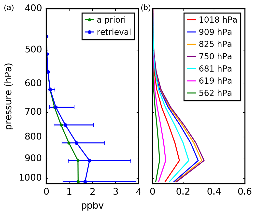
Figure 1 CrIS ammonia retrieval at 42.21^∘ N, 70.82^∘ W on 12 May 2016, 17:31:59 UTC. Panel (a) shows the retrieval and a priori profiles, while panel (b) shows the rows of the averaging kernel for the seven vertical levels closest to the surface. The number of degrees of freedom for this retrieval is 0.96.

For the emissions inversions, we utilized CrIS retrievals within the GEM-MACH regional domain, which consists mostly of North America. Additionally, we only consider retrievals over land. As a quality control measure, we only use CrIS ammonia retrievals that have a signal-to-noise ratio of at least 1 and have at least 0.1 degrees of freedom.

The inversions in this work use retrievals between May and August 2016, when the ammonia signal is relatively strong, as to maximize the number of CrIS retrievals that have an adequately large signal-to-noise ratio. The particular months chosen also reflect the availability of required input files for GEM-MACH. The year 2016 was chosen in part due to the relatively low number of forest fires during this year (Munoz-Alpizar et al., 2017; Earl and Simmonds, 2018) to decrease the chances of misattributing elevated ammonia levels due to forest fires with other emission sources. While we seek to minimize the effect of forest fires on the emissions inversions in this work, in other contexts this might not be necessary or desirable. For example, if the emissions are only used for the time period when the fire occurred, having the fires affect the inversion may be advantageous.

During the course of this work, an issue related to accounting for the non-detection of ammonia in the CrIS spectrum was identified, which primarily affected the CrIS data in non-source regions (e.g. high northern latitudes). As these locations were not areas of interest for this work, only observations south of 60^∘ N were used in this study. While non-detects have been accounted for in newer versions of the CrIS ammonia product (White et al., 2021), these corrections were only made available after the completion of this study.

Although CrIS provides twice-daily ammonia observations, the uncertainties on individual retrievals are relatively large (Shephard and Cady-Pereira, 2015). Thus, while inversions on the timescale of a day could be performed, increasing the number of observations used in a single inversion by increasing the time window of the inversion can mitigate the large uncertainties on individual retrievals. Accordingly, each inversion used a whole month's worth of CrIS retrievals and yielded an estimate of the monthly mean ammonia emissions. The total number of retrievals used for each inversion and their spatial distribution are shown in Fig. S1 in the Supplement. The selection process described in the previous paragraphs resulted in 70 %–85 % of the retrievals used in the inversions coming from daytime retrievals.

2.2 Surface air quality observations

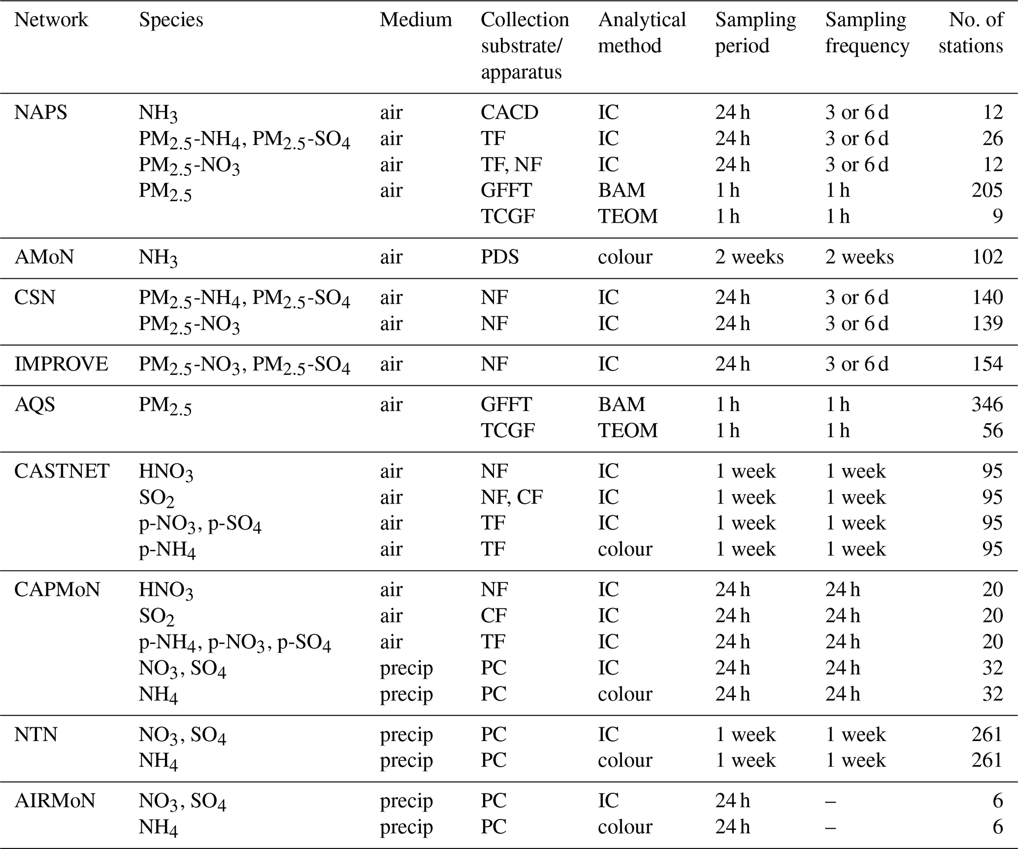
The GEM-MACH surface fields predicted using the original emissions and those from the inversions were compared to surface observations from various observation networks. In addition to ammonia observations, to examine the impact of the inversion-based emission changes on inorganic PM formation, observations of nitric acid (HNO₃), sulfur dioxide, ammonium (${\mathrm{NH}}_{\mathrm{4}}^{+}$), nitrate (${\mathrm{NO}}_{\mathrm{3}}^{-}$), and sulfate (${\mathrm{SO}}_{\mathrm{4}}^{\mathrm{2}-}$) were also considered. For the aerosol species, we distinguish observations of the total concentration over all particle sizes (p-NH₄, p-NO₃, and p-SO₄ for ammonium, nitrate, and sulfate, respectively) from observations only measuring the PM_2.5 component (PM_2.5-NH₄, PM_2.5-NO₃, and PM_2.5-SO₄ for ammonium, nitrate, and sulfate, respectively). A summary of these observations is shown in Table 1, and site locations are shown in Fig. S2.

The Ammonia Monitoring Network (AMoN; https://nadp.slh.wisc.edu/networks/ammonia-monitoring-network/, last access: 29 April 2022) is one of several monitoring networks that are part of the US National Atmospheric Deposition Program (NADP), with most sites located in the US. AMoN monitors ammonia levels using Radiello^® passive diffusion samplers that are deployed for 2-week periods. Canada's National Air Pollution Surveillance (NAPS; https://www.canada.ca/en/environment-climate-change/services/air-pollution/monitoring-networks-data/national-air-pollution-program.html, last access: 29 April 2022) network provides observations of a variety of pollutants, including ammonia, within Canada. NAPS uses a citric-acid-coated denuder to collect ammonia samples over a 24 h period every 3 or 6 d.

Both the US Environmental Protection Agency's (EPA) Clean Air Status and Trends Network (CASTNET; https://www.epa.gov/castnet, last access: 29 April 2022) and ECCC's Canadian Air and Precipitation Monitoring Network (CAPMoN; https://www.canada.ca/en/environment-climate-change/services/air-pollution/monitoring-networks-data/canadian-air-precipitation.html, last access: 29 April 2022) use three-stage filter packs to collect HNO₃, SO₂, p-NH₄, p-NO₃, and p-SO₄. There are currently two major networks in the US that monitor speciated PM_2.5 levels: the US EPA's Chemical Speciation Network (CSN; https://www.epa.gov/amtic/chemical-speciation-network-csn, last access: 29 April 2022) and the Interagency Monitoring of PROtected Visual Environments (IMPROVE; http://vista.cira.colostate.edu/Improve, last access: 29 April 2022) network (partnership between the US EPA, US National Park Service, and other federal, state, and tribal agencies). CSN has a mission focused on air quality and has stations primarily located in urban settings, while IMPROVE concentrates on visibility and has stations mainly in rural locations. CSN and IMPROVE both use nylon filters to collect PM_2.5-NO₃ and PM_2.5-SO₄ (and PM_2.5-NH₄ in the case of CSN). Speciated PM_2.5 observations are also measured at NAPS sites, with PM_2.5-NH₄, PM_2.5-NO₃, and PM_2.5-SO₄ collected by Teflon filters. NAPS also provides hourly observations of total PM_2.5. Additional hourly total PM_2.5 measurements are supplied by the EPA's Air Quality System (AQS; https://www.epa.gov/airdata, last access: 29 April 2022), which collects data from EPA and state, local, and tribal agencies.

Precipitation–chemistry concentration measurements for ammonium, nitrate, and sulfate were also examined. Observations from two NADP networks were considered: the National Trends Network (NTN; https://nadp.slh.wisc.edu/networks/national-trends-network/, last access: 29 April 2022) and the Atmospheric Integrated Research Monitoring Network (AIRMoN; http://nadp2.slh.wisc.edu/airmon/, last access: 29 April 2022). Although the AIRMoN program ceased operations in 2019, observations from this network were available for 2016, the year examined in this work. Precipitation–chemistry measurements in Canada were provided by the CAPMoN network.

Table 1 Surface observations used in this study. Collection substrate/apparatus types include Teflon filter (TF), nylon filter (NF), K₂CO₃-impregnated cellulose filter (CF), Teflon-coated glass fiber filter (TCGF), glass fiber filter tape (GFFT), citric-acid-coated denuder (CACD), passive diffusion sampler (PDS), and precipitation collectors (PC). Analytical methods include ion chromatography (IC), colorimetry (colour), beta attenuation monitoring (BAM), and tapered element oscillating microbalance (TEOM). AIRMoN precipitation samples are collected within 24 h of the start of a precipitation event.

To evaluate the predicted fields from GEM-MACH against these surface observations, we examine the changes in the normalized mean bias (NMB), normalized standard deviation of differences (NSTD), and the Pearson correlation coefficient (ρ) between GEM-MACH and the observations, defined by

$$\begin{array}{}\text{(1a)}& {\displaystyle }\text{NMB}={\displaystyle \frac{\mathrm{100}\mathit{\%}}{\stackrel{\mathrm{‾}}{O}}}\times {\displaystyle \frac{\mathrm{1}}{N}}\sum _i^N(M_i-O_i),\text{(1b)}& {\displaystyle }\mathrm{\text{NSTD}}={\displaystyle \frac{\mathrm{100}\mathit{\%}}{\stackrel{\mathrm{‾}}{O}}}\times \sqrt{{\displaystyle \frac{\mathrm{1}}{N-\mathrm{1}}}\sum _i^N{\left(M_i-O_i-\stackrel{\mathrm{‾}}{M}+\stackrel{\mathrm{‾}}{O}\right)}^{\mathrm{2}}},\text{(1c)}& {\displaystyle }\mathit{\rho }={\displaystyle \frac{{\sum }_i^N\left(M_i-\stackrel{\mathrm{‾}}{M}\right)(O_i-\stackrel{\mathrm{‾}}{O})}{\sqrt{{\sum }_i^N{\left(M_i-\stackrel{\mathrm{‾}}{M}\right)}^{\mathrm{2}}}\sqrt{{\sum }_i^N{\left(O_i-\stackrel{\mathrm{‾}}{O}\right)}^{\mathrm{2}}}}},\text{(1d)}& {\displaystyle }\stackrel{\mathrm{‾}}{O}={\displaystyle \frac{\mathrm{1}}{N}}\sum _i^N{O}_i,\text{(1e)}& {\displaystyle }\stackrel{\mathrm{‾}}{M}={\displaystyle \frac{\mathrm{1}}{N}}\sum _i^N{M}_i,\end{array}$$

where O_i and M_i are the ith observation and its corresponding model value, respectively, and N is the number of observations. Some observations from networks that have a sampling period of a week or longer (AMoN, CASTNET, NTN) straddled 2 months, i.e. started at the end of one month and finished at the beginning of the next month. For monthly statistics of concentration observations, if an observation had at least 4 d within a month it is included in the statistics calculation for that month. For precipitation–chemistry concentration observations, observations straddling months are not included in the monthly statistics.

2.3 The GEM-MACH model

GEM-MACH (Moran et al., 2010; Gong et al., 2015; Pavlovic et al., 2016; Pendlebury et al., 2018), ECCC's operational air quality model, is an online chemical transport model embedded within the Global Environmental Multiscale (GEM) model (Côté et al., 1998b, a; Girard et al., 2014), ECCC's operational weather forecasting model. GEM-MACH augments the GEM model by adding tropospheric gas-phase, aqueous-phase, and inorganic heterogeneous chemistry to the model.

Both regional and global versions of GEM-MACH are available. We use version 2.4.6-LTS.17 of the regional GEM-MACH model (Moran et al., 2018, 2019), which is based on version 4.8-LTS.17 of GEM (Girard et al., 2014). The model domain encompasses Canada, the United States, and northern Mexico. The horizontal grid has a spacing of 0.09^∘ (∼ 10 km), while the vertical grid has 80 hybrid log hydrostatic pressure levels on a Charney–Phillips staggered grid (Charney and Phillips, 1953; Girard et al., 2014) that extends from the surface to 0.1 hPa. In this work, GEM-MACH is run with sequential 12 h forecasts, where the meteorological fields are refreshed at the beginning of each forecast using analyses from ECCC's Regional Deterministic Prediction System (RDPS) (Caron et al., 2015).

The gas-phase chemistry in GEM-MACH is modelled using the ADOM-II mechanism (Stockwell and Lurmann, 1989; Stroud et al., 2008). The gas-phase dry deposition scheme is based on the unidirectional “big leaf” resistance model of Zhang et al. (2002). While this unidirectional model is currently used in the operational version of GEM-MACH, recently a bidirectional flux model for ammonia has been added to GEM-MACH (Whaley et al., 2018). The use of this bidirectional flux scheme instead of the unidirectional model will be the subject of future work. Particle dry deposition and gravitational settling is modelled using the scheme of Zhang et al. (2001), and the wet deposition scheme is described in Gong et al. (2006).

The aerosol chemical components considered by GEM-MACH are sulfate, nitrate, ammonium, elemental carbon, crustal material, sea salt, primary and secondary organic aerosols, and H₂O. GEM-MACH uses a sectional representation of the PM size distribution and currently can be run with either 2 or 12 size bins. While the two-bin model only gives limited information about the aerosol size distribution (one 0–2.5 µm fine size bin and one 2.5–10 µm coarse-fraction bin), it offers increased computational speed and reduced memory requirements compared to the 12-bin model. Currently, the operational version of GEM-MACH runs the two-bin version of the model. As this work will in part be used to evaluate the potential use of CrIS ammonia retrievals in an operational air-quality model, the two-bin model was used for this work.

Inorganic heterogeneous chemistry is implemented in GEM-MACH using the HETV code (Makar et al., 2003), based on the ISORROPIA model (Nenes et al., 1998), which computes the gas–aerosol phase partitioning for the sulfate–nitrate–ammonium system. HETV computes this partitioning using the assumption of equilibrium to determine the abundances of NH₃(g), HNO₃(g), ${\mathrm{NO}}_{\mathrm{3}}^{-}\left(\mathrm{aq}\right)$, ${\mathrm{SO}}_{\mathrm{4}}^{\mathrm{2}-}\left(\mathrm{aq}\right)$, ${\mathrm{NH}}_{\mathrm{4}}^{+}\left(\mathrm{aq}\right)$, ${\mathrm{HSO}}_{\mathrm{4}}^{-}\left(\mathrm{aq}\right)$, NH₄NO₃(s), NH₄HSO₄(s), (NH₄)₃H(SO₄)₂(s), and (NH₄)₂SO₄(s). While the HETV code computes the partitioning for all of the aforementioned species, for the aqueous- and solid-phase species, only the total mass of sulfate, nitrate, and ammonium within each size bin is retained in GEM-MACH after HETV is run. To offset the relatively large computational expense of the heterogeneous chemistry done by HETV, HETV computes the gas–aerosol partitioning using a single “bulk” calculation using the total mass of each species over all aerosol bin sizes. Following this bulk calculation, the change in bulk mass is distributed to the different size bins using ratios of gas-to-particle diffusion rates, computed via the formulation of Fuchs and Sutugin (1970) (see also Makar et al., 1998).

Emissions are supplied to GEM-MACH via hourly, gridded, speciated emissions files. These emissions files were created using the Sparse Matrix Operator Kernel Emissions (SMOKE; https://www.cmascenter.org/smoke, last access: 29 April 2022) processing system, which assigns temporal profiles, spatial surrogate fields, and speciation profiles based on source type to monthly or annual anthropogenic emissions inventories (Moran et al., 2018). The base case model run in this study used the set of emissions used by the operational version of GEM-MACH at the time of writing (version 3.1.2 of this emissions data set). These emissions were constructed using a 2013 Canadian emissions inventory from Canada's Air Pollutant Emissions Inventory (https://www.canada.ca/en/environment-climate-change/services/pollutants/air-emissions-inventory-overview.html, last access: 29 April 2022), a 2017 US projected inventory obtained from the EPA's Air Emissions Modeling 2011 Platform (version 6.3; https://www.epa.gov/air-emissions-modeling/2011-version-63-platform, last access: 29 April 2022), and a 2008 Mexican inventory also obtained from the EPA's Air Emissions Modeling 2011 Platform (version 6.2; https://www.epa.gov/air-emissions-modeling/2011-version-62-platform, last access: 29 April 2022). While not done in this study, these inventory-based emissions can be supplemented by other emissions types, such as forest fire emissions (Pavlovic et al., 2016; Chen et al., 2019).

3 Emissions inversion procedure

This section details different aspects of the inversion process. First, the ensemble-variational algorithm used to perform the emissions inversions is described. This is followed by a description of the ensemble used in the inversions. Lastly, a novel method for comparing model profiles to satellite retrievals in the inversion algorithm is developed.

3.1 The ensemble-variational method

Variational methods solve inverse problems through the minimization of a cost function to obtain an updated solution, known as the analysis, which is a statistical blend of observational and background (a priori or “first-guess”) information. The relative influence the observational and background information have on the analysis is dictated by the specification of error covariances for the observations and background. Ensemble-variational techniques, commonly referred to as EnVar, use an ensemble of model states to model the background error covariance. In this section (and Appendix A), we review the EnVar method and apply it to an emissions inversion.

Most variational methods solve for the additive field that yields the analysis, referred to as the increment, instead of the analysis itself. In our case, we seek the atmospheric ammonia concentration increment vector Δc that minimizes the cost function J defined by

$$\begin{array}{}\text{(2)}& J={\displaystyle \frac{\mathrm{1}}{\mathrm{2}}}\mathbf{\Delta }{\mathit{c}}^{\mathrm{T}}{\mathbf{B}}_{\text{cc}}^{-\mathrm{1}}\mathbf{\Delta }\mathit{c}+{\displaystyle \frac{\mathrm{1}}{\mathrm{2}}}{\left(\mathit{d}-\mathbf{H}\mathbf{\Delta }\mathit{c}\right)}^{\mathrm{T}}{\mathbf{R}}^{-\mathrm{1}}\left(\mathit{d}-\mathbf{H}\mathbf{\Delta }\mathit{c}\right),\end{array}$$

where B_cc is the atmospheric concentration background error covariance matrix and R is the observation error covariance matrix. The vector $\mathit{d}=\mathit{y}-H\left({\mathit{c}}^{\mathrm{b}}\right)$, known as the innovation, is the difference between the observations y and the background concentration c^b input into the observation operator H. The observation operator H, and its linearization H that appears in Eq. (2), relates the atmospheric concentrations to the observations. For the cost function given in Eq. (2), the first term measures the mismatch between the model state and the background, while the second term measures the mismatch between the model state and the observations.

The atmospheric concentrations produced by a model are dependent on the emissions as well as many other factors such as meteorology, initial conditions, and boundary values. For simplicity, in this work we assume that the uncertainty in the atmospheric concentrations is due solely to the uncertainty in emissions and neglect all other sources of uncertainty, such as that from meteorology and chemistry. We also assume that our observations are of the atmospheric chemical concentrations only and do not directly measure emissions. In this situation, we can use the properties of analysis splitting to relate the increment in the unobserved emissions vector Δe to the increment in the observed concentrations Δc by (Ménard et al., 2019)

$$\begin{array}{}\text{(3)}& \mathbf{\Delta }\mathit{e}={\mathbf{B}}_{\text{ec}}{\mathbf{B}}_{\text{cc}}^{-\mathrm{1}}\mathbf{\Delta }\mathit{c},\end{array}$$

where B_ec is the error cross-covariance between the emissions and the atmospheric concentrations. We define e and its increment Δe to allow them to represent either the emissions directly or a parameterization of the emissions, which will be elaborated on in the next section. The details of the minimization of the cost function in Eq. (2) and the subsequent transformation to the emissions increment in Eq. (3) are given in Appendix A.

Ensemble-variational methods use an ensemble of states to model the background error covariances. The background error covariances can originate solely from an ensemble, as done in this work, or can be a hybrid that combines ensemble information with information from other sources. For this work, we use an ensemble of 100 members, with each ensemble member i consisting of a perturbed emissions field δe_i and a corresponding perturbed concentration field δc_i generated by running GEM-MACH with the perturbed emissions. The way in which the emissions were perturbed will be described in the following section.

To minimize the effect of spurious long-distance correlations due to a small ensemble size, as well as to increase the rank of the background error covariance matrix, the concentrations and emissions background error covariances are localized via the Hadamard (element-wise) product with localization matrices L_cc and L_ee, respectively (see Appendix A for more details). For the concentrations, we use a localization L_cc that is separable in the horizontal and the vertical. We construct L_ee and the horizontal component of L_cc from homogeneous and isotropic functions with correlations modelled with the fifth-order function of Gaspari and Cohn (1999). We choose L_cc and L_ee to have horizontal correlations with half-widths at half-maximum of 120 and 100 km, respectively, and L_cc to have vertical correlations with a half-width at half-maximum of 3 km. These values were chosen to be moderately larger than estimates of the distances travelled during the atmospheric lifetime of ammonia (Dammers et al., 2019).

3.2 Emissions parameterization and ensemble construction

As mentioned in Sect. 2.1, the inversions performed in this study solve for monthly mean ammonia emissions, which were specified on the same horizontal grid used for the GEM-MACH emissions (∼ 10 km resolution). In emissions inversion studies, it is common to use a parameterization of the emissions, as it may be advantageous to solve for the parameterization variables instead of the emissions directly. Additionally, a parameterization of the emissions may be convenient for generating the ensemble of emissions required for the ensemble-variational inversion. The use of such a parameterization for both of the aforementioned purposes is discussed in this section.

In Sect. 3.1, we defined e flexibly to allow it to represent either the emissions directly or a parameterization of the emissions. Here we denote the actual emissions with E to differentiate it from a (possible) parameterization variable e and define E⁽⁰⁾ and E⁽¹⁾ as the original and updated/perturbed emissions, respectively. As our inversions solve for monthly mean ammonia emissions, E⁽⁰⁾ represents the original monthly mean ammonia emissions (described in Sect. 2.3), and E⁽¹⁾ represents either the posterior or perturbed monthly emissions (depending on context). If no parameterization is used then we have $E^{\left(\mathrm{1}\right)}=E^{\left(\mathrm{0}\right)}+\mathrm{\Delta }e$. Often a scaling factor is used to parameterize the emissions, most often in a linear ($E^{\left(\mathrm{1}\right)}=(\mathrm{1}+\mathrm{\Delta }e)E^{\left(\mathrm{0}\right)}$) or exponential (E⁽¹⁾=exp (Δe)E⁽⁰⁾) form. One benefit of the exponential scaling form is that the scaling factor is positive for all values of Δe.

An initial comparison of the CrIS ammonia retrievals to GEM-MACH suggested that the processed ammonia emissions inventories described in Sect. 2.3 were missing emission sources in some locations. As the processed emissions inventory at these locations may have a negligible value, if a scaling factor parameterization is used, an extremely large scaling factor value may have to be applied at these locations to achieve an adequately large posterior emissions value. As very large scaling values may cause numerical difficulties within the inversion computation, inversions that use scaling factor parameterizations often impose an upper bound on the scaling factor value, which in practice restricts the inversion to modifying only previously known emission sources.

To allow the inversion to add previously unknown emission sources, as well as restrict the emissions to positive values, we use an alternative emissions parameterization, given by

$$\begin{array}{}\text{(4)}& \begin{array}{rl}& E^{\left(\mathrm{1}\right)}(E^{\left(\mathrm{0}\right)},\mathrm{\Delta }e)\\ & =\left\{\begin{array}{ll}{E}^{\left(\mathrm{0}\right)}+\mathrm{\Delta }e& E^{\left(\mathrm{0}\right)}+\mathrm{\Delta }e\ge \mathit{\epsilon }\\ \mathit{\epsilon }{\left(E^{\left(\mathrm{0}\right)}/\mathit{\epsilon }\right)}^{(E^{\left(\mathrm{0}\right)}+\mathrm{\Delta }e-\mathit{\epsilon })/(E^{\left(\mathrm{0}\right)}-\mathit{\epsilon })}& \text{otherwise}\end{array},\right.\end{array}\end{array}$$

where the variable Δe parameterizes the emissions and ε is a positive constant. When E⁽⁰⁾+Δe is larger than ε, Δe acts as a linear perturbation, which avoids the missing-source scaling problem described above. To avoid negative emissions values, if E⁽⁰⁾+Δe is smaller than ε, then the initial emissions E⁽⁰⁾ are exponentially damped. The exponential dampening parameters were chosen so that the function E⁽¹⁾(E⁽⁰⁾,Δe) is continuous and has $E^{\left(\mathrm{1}\right)}(E^{\left(\mathrm{0}\right)},\mathrm{\Delta }e=\mathrm{0})=E^{\left(\mathrm{0}\right)}$ for all values of E⁽⁰⁾. We choose a value of 0.1 g s⁻¹ per cell (∼0.026 kg ha⁻¹ per month) for the constant ε (see Fig. 3 for comparison to monthly mean emissions).

Inversions based on ensemble-variational methods use an ensemble to approximate the full error covariance associated with our a priori knowledge of the model state. The ensemble of emissions were generated as follows: for each ensemble member i, a 2D random field δe_i(x_j) is generated at each grid point j (with position x_j). The random field δe_i(x_j), along with the original monthly mean ammonia emissions E⁽⁰⁾(x_j), is used in Eq. (4) to yield a perturbed monthly mean ammonia emissions field $E_i^{\left(\mathrm{1}\right)}\left({\mathit{x}}_j\right)=E^{\left(\mathrm{1}\right)}\left(E^{\left(\mathrm{0}\right)}\right({\mathit{x}}_j),\mathrm{\Delta }e=\mathit{\delta }{e}_i({\mathit{x}}_j\left)\right)$ at each grid point j for each ensemble member. The ensemble of atmospheric chemical concentrations is then gained by generating hourly emissions for each member by applying the same temporal profiles as described in Sect. 2.3 to the perturbed monthly mean emissions and then running GEM-MACH with each set of hourly emissions.

The distribution from which the random fields δe are drawn determines the emissions background error covariance B_ee. As is often the case in inversion/assimilation work, deriving background error covariances that accurately specify the uncertainties of our a priori knowledge of the emissions is difficult. For simplicity, to create our ensemble of emissions we draw δe from an isotropic normal distribution with a correlation half-width at half-maximum of 40 km. We set the standard deviations of this distribution to be 50 % of the monthly mean values from the processed emissions inventory, but we impose a minimum standard deviation value of 1 g s⁻¹ per cell (∼ 0.26 kg ha⁻¹ per month) so that areas without previously known emissions sources have a non-negligible ensemble variance.

3.3 Comparison between model profiles and satellite retrievals

Variational inversion methods, such as the ensemble-variational method described in Sect. 3.1, rely on a comparison of a model with observations to generate an optimized state, done through the computation of the innovation $\mathit{d}=\mathit{y}-H\left({\mathit{c}}^{\mathrm{b}}\right)$. For some observation data sets, such as many in situ observations, performing this comparison is trivial. But for some remotely sensed observations, added complications can arise that make this comparison more difficult. In this section, we develop a new hybrid approach for comparing the CrIS ammonia retrievals to model profiles for use in an inversion system.

The CrIS ammonia retrievals are performed with the logarithm of concentrations, which can be represented by (Rodgers, 2000)

$$\begin{array}{}\text{(5)}& \ln \left({\mathit{c}}^{\mathrm{r}}\right)={\mathbf{A}}^{\text{log}}\ln \left(\mathit{c}\right)+\left(\mathbf{I}-{\mathbf{A}}^{\text{log}}\right)\ln \left({\mathit{c}}^{\mathrm{a}}\right)+\mathbf{G}\mathit{ϵ},\end{array}$$

where c, c^r, and c^a are the true, retrieved, and a priori volume mixing ratio profiles in parts per million by volume, respectively; A^log is the averaging kernel in log-space; G is the gain matrix (quantifies the sensitivity of the retrieval to the observation); and ϵ is the total error. By replacing the true atmospheric profile c with the model profile c^b, neglecting the noise term Gϵ, and taking the exponential of both sides of Eq. (5), one can construct an observation operator H^log that maps the model profile into a quantity that can be directly compared to the CrIS ammonia retrieval as

$$\begin{array}{}\text{(6)}& {\left[H^{\text{log}}\left(c^{\mathrm{b}}\right)\right]}_i=\prod _j{\left(c_j^{\mathrm{b}}\right)}^{A_{i,j}^{\text{log}}}\times {\left(c_j^{\mathrm{a}}\right)}^{{\mathit{\delta }}_{i,j}-A_{i,j}^{\text{log}}},\end{array}$$

where i,j indexes the vertical levels of the profiles, δ_i,j is the Kronecker delta function, and H^log(c^b) has units of parts per million by volume. With this observation operator, the model equivalent to the retrieved profile is a product of profiles, raised to a power determined by the averaging kernel.

While the observation operator in Eq. (6) functions well in many situations, problems may occur when part of the model profile c^b is either zero or negligibly small. As the operator in Eq. (6) is a product of model profile terms, if the model profile is zero at any point in the profile, the whole product will be zero unless the corresponding component of the averaging kernel is exactly zero (or will approach an infinite value if the averaging kernel component is negative). This will occur regardless of the values elsewhere in the model profile. An example of this behaviour can be seen in Fig. 2, where the model profile c^b shown has non-negligible values below ∼ 680 hPa but values of zero above ∼ 600 hPa. Consequently, using Eq. (6) maps this model profile to the profile H^log(c^b), which is zero at all vertical levels. As the H^log(c^b) profile would be the same regardless of the model values below ∼ 680 hPa, this observation operator may be problematic when comparing model profiles to retrievals since H^log(c^b) in this case will be completely insensitive to the amount of ammonia in the model at lower levels.

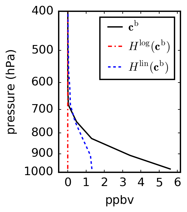
Figure 2 GEM-MACH profile at a retrieval location for the CrIS retrieval at 44.92^∘ N, 92.96^∘ W on 12 May 2016, 07:48:58 UTC. Profiles are shown for the model (c^b), as well as the profiles that result from applying the log-space (H^log) and linear-space (H^lin) observation operators.

To alleviate this issue, one might attempt to truncate these profiles to cut off all levels where the model profile is zero (or very small). However, it was observed that when GEM-MACH is used with the emissions inventory described in Sect. 2.3, in these situations the vertical levels at which the model profile is zero or very small often corresponded to levels where the averaging kernel is non-negligible and in some cases even peaks at these levels. Therefore, truncating the profiles in this manner would remove important vertical levels in the retrieval. Alternatively, one could retain all vertical levels but impose some model profile minimum value, so that the terms in the product in Eq. (6) are multiplied by a small value instead of zero, yielding a non-zero value for H^log(c^b). But in this case, H^log(c^b) would primarily be determined by the somewhat arbitrarily chosen lower-bound value and would be relatively insensitive to the amount of ammonia in the model.

An observation operator that can avoid this problem is the linearization of Eq. (5), which can be written as

$$\begin{array}{}\text{(7)}& H^{\text{lin}}\left({\mathit{c}}^{\mathrm{b}}\right)={\mathbf{A}}^{\text{lin}}{\mathit{c}}^{\mathrm{b}}+(\mathbf{I}-{\mathbf{A}}^{\text{lin}}){\mathit{c}}^{\mathrm{a}},\end{array}$$

where A^lin is the averaging kernel linearized in c^b−c^a. As H^lin(c^b) is linear in c^b instead of containing products of profiles, the zero-valued profiles that are produced with H^log(c^b) are avoided. This is illustrated in Fig. 2, where c^b is mapped to a non-zero profile H^lin(c^b).

While using the linearized averaging kernel may avoid some of the problems encountered when using the log-space averaging kernel, the linearized averaging kernel may only be a good approximation when the difference between the model and a priori profiles is small. As only three a priori profiles are used in the CrIS ammonia retrieval, this will often not be the case. One might consider only using the linearization when the difference between the model and a priori profiles is small, but this will likely be very restrictive and would exclude many profiles of interest, in particular cases where the model is significantly smaller than the selected a priori. On the other hand, using the linearization in all cases could introduce new biases into the comparison. For instance, when H^lin(c^b) is compared to H^log(c^b) for cases where H^log(c^b) is not zero at all levels, H^lin(c^b) is systematically overestimated compared to H^log(c^b) and can introduce biases on the order of 0.5 ppbv.

To balance these different factors, we propose using a hybrid log–linear observation operator that attempts to choose the best method according to the particular situation. To assess which method to use, for each retrieval we compute the total column value of the model profile X(c^b) and the total column value of its log-space mapped profile X(H^log(c^b)), where X(⋅) is the total column operator. We associate cases where the log-space observation operator has zeroed out a non-negligible model profile with model profiles that have a total column value X(c^b) above some specified minimum threshold value X_min, as well as a maximum profile value above some minimum value c_min, but that have a X(H^log(c^b)) value that is below X_min. If these criteria determine that the model profile has been zeroed out, then the linearized observation operator is used, otherwise the log-space observation operator is used.

Most of the vertical distribution information in the CrIS ammonia retrieval originates from a priori information, so for computational simplicity, we use the total column values computed from each profile for the comparison of the model to the retrieval in the inversion. However, we emphasize that the full averaging kernel over all vertical levels is nevertheless utilized. In summary, the CrIS retrieval is compared to the GEM-MACH model by computing the difference between the total column of the CrIS retrieval and the GEM-MACH model profile used in the piece-wise function

$$\begin{array}{}\text{(8)}& \begin{array}{rl}& H\left({\mathit{c}}^{\mathrm{b}}\right)\\ & =\left\{\begin{array}{ll}X\left(H^{\text{lin}}\right({\mathit{c}}^{\mathrm{b}}\left)\right)& X_{min}<X\left({\mathit{c}}^{\mathrm{b}}\right)\text{and}\\ & X\left(H^{\text{log}}\right({\mathit{c}}^{\mathrm{b}}\left)\right)\le X_{min}\text{and}\\ & c_{min}<max\left({\mathit{c}}^{\mathrm{b}}\right)\\ X\left(H^{\text{log}}\right({\mathit{c}}^{\mathrm{b}}\left)\right)& \text{otherwise}\end{array},\right.\end{array}\end{array}$$

where H^log(c^b) and H^lin(c^b) are calculated from Eqs. (6) and (7), respectively. We choose the minimum threshold values used in Eq. (8) as X_min = 10¹⁴ $\mathrm{molec}.{\mathrm{cm}}^{-\mathrm{2}}$ and c_min = 0.1 ppbv. In the remainder of the paper, we refer to this as the “hybrid” method. Details of the performance of the hybrid method can be found in Appendix B.

Lastly, to account for errors in the observation operator (from errors related to the issues discussed above as well as any other representation errors), the total column error variances as diagnosed by Shephard and Cady-Pereira (2015) were scaled by a factor of 100 to form the diagonal terms of R used in the inversions (similar to the regularization used in Cao et al., 2020).

4 Results

In this section we discuss the results of the emissions inversions and their impact on predicted fields in GEM-MACH. Section 4.1 focuses on the results from the inversions and their impact on the surface ammonia in GEM-MACH. Section 4.2 and 4.3 examine the effect on PM formation and the PM size distribution in GEM-MACH, respectively, while Sect. 4.4 considers the impact on deposition.

4.1 Ammonia emissions inversions and predicted surface concentrations

4.1.1 Emissions inversions

The monthly mean ammonia emissions for the original set of emissions is shown in the left column of Fig. 3. The emissions generally coincide with areas with significant agricultural activities, with significant emissions originating from regions such as the American Midwest, California's Central Valley, and the Canadian prairie provinces. For the emissions inventory in May, total fertilizer and livestock emissions for the contiguous US are roughly equal to one another, while total Canadian fertilizer emissions are roughly 50 % larger than Canadian livestock emissions. But for June to August, the inventory emissions are dominated by livestock emissions for both the contiguous US and Canada. Total ammonia emissions for the contiguous US and Canada are shown in Table 2.

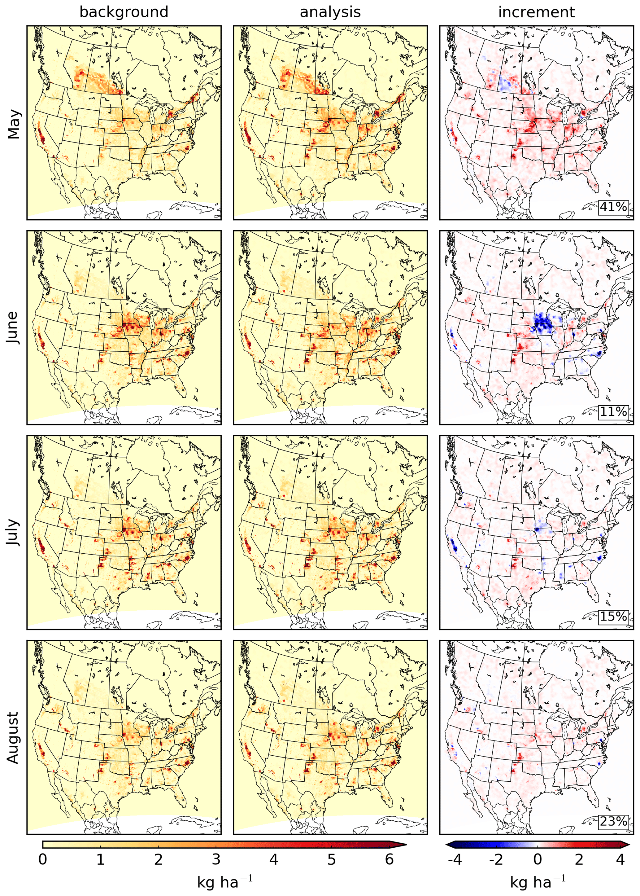
Figure 3 Monthly ammonia emissions for May to August 2016 on the GEM-MACH model grid. The left column shows the original set of emissions (the background) that are described in Sect. 2.3. The middle column shows the emissions produced by the inversions (the analysis), while the right column shows the difference between the two (the increment). For plots on the right, the percentages in the lower right corner show the change over the whole domain.

Table 2 Total monthly ammonia emissions (in kilotonnes) for the original and updated sets of emissions for the contiguous US and Canada.

The ammonia total columns from the CrIS retrievals and their analogous quantities from GEM-MACH run using the original ammonia emission for May to August 2016 are displayed in Fig. 4, which shows monthly mean column values binned on the GEM-MACH grid. Their differences (the innovations) are shown in the right column. In this figure, the GEM-MACH columns are derived using the hybrid observation operator of Sect. 3.3, and, unless stated otherwise, results in this section will be shown for comparisons using this observation operator. For the innovation plots, each difference i within a cell is weighted by ${\mathit{h}}_i{\mathbf{B}}_{\text{cc}}{\mathit{h}}_i^{\mathrm{T}}/({\mathit{h}}_i{\mathbf{B}}_{\text{cc}}{\mathit{h}}_i^{\mathrm{T}}+R_{i,i})$ in the computation of the mean for that cell, where h_i is the ith row of the matrix H, to approximate the weight given to that difference in the inversion (this roughly approximates the Kalman gain in observation space). From the right column of Fig. 4, it is apparent that while the GEM-MACH column values are larger than the CrIS retrievals in some places, such as the American Midwest, eastern North Carolina, and California's Central Valley in June and July, the CrIS retrieval columns are larger than the GEM-MACH values in most other locations within the domain. The largest differences between the CrIS retrieval columns and GEM-MACH columns occur in the central continental US from the American Midwest to northern Texas, California, and the Canadian prairie provinces.

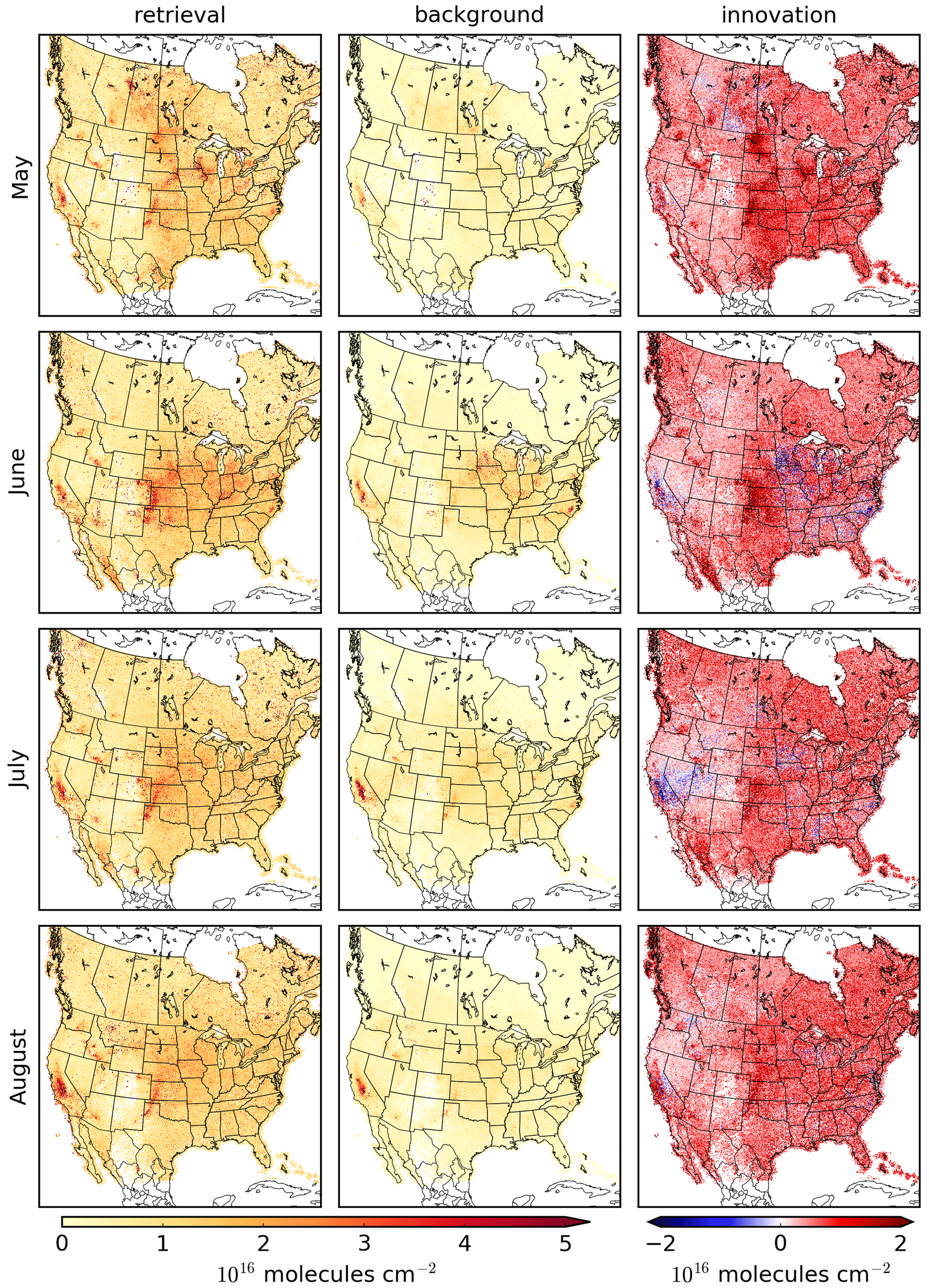
Figure 4 Monthly mean ammonia total columns for the CrIS retrievals (left column) compared to the analogous quantities for GEM-MACH run using the original set of emissions (the background, middle column), as well as their difference (innovation, right column), for May to August 2016. The GEM-MACH columns are calculated using the hybrid method given in Eq. (8). The values plotted are monthly means binned on the GEM-MACH grid. For plots of the innovation, each difference i within a cell is weighted by ${\mathit{h}}_i{\mathbf{B}}_{\text{cc}}{\mathit{h}}_i^{\mathrm{T}}/({\mathit{h}}_i{\mathbf{B}}_{\text{cc}}{\mathit{h}}_i^{\mathrm{T}}+R_{i,i})$ in the computation of the mean for that cell.

The ammonia emissions inversions for May to August 2016 are shown in Fig. 3, where the monthly mean emissions resulting from the inversions are shown in the middle column, and the differences between the emissions from the inversion and the original emissions are shown in the right column. The total change in emissions from the inversion over the contiguous US and Canada is shown in Table 2. In Fig. 3 and in subsequent figures within this section, the percentages shown in the lower right corner of model difference plots show the total difference over the model domain. Under the assumptions detailed in Sect. 3.1, the inversion attributes all differences between the original GEM-MACH run and the CrIS retrievals to the ammonia emissions. Accordingly, as the CrIS ammonia retrievals are larger than the GEM-MACH values in most of the model domain, the inversion increases ammonia emissions in most places within the domain as well. The largest change in emissions occurs in May, where emissions over the domain increase by 41 %, although the relative change in emissions in Canada for June to August is larger than that for May. The spatial distribution of the emissions increment generally agrees with those found in Cao et al. (2020), who attributed the underestimations of emissions seen in much of the contiguous US to underestimations in emissions from both fertilizers and livestock (depending on location).

Although the inversions increase ammonia emissions in much of the domain, some notable exceptions to this are in southern Minnesota and Iowa, California's Central Valley, and eastern North Carolina for the months of June and July. These correspond to areas with large agricultural industries (most significantly cattle in the Central Valley and swine in southern Minnesota, northern Iowa, and eastern North Carolina) and represent significant emissions sources in the a priori emissions. The overestimations of emissions in June and July in these locations were also found by Cao et al. (2020) for 2014.

In a few locations within the model domain, the inversion decreased emission sources in some months while it increased it in other months. For example, emissions were decreased in much of southern Minnesota and Iowa in June and July but were increased in those areas in May and August. A similar time-dependent behaviour is also seen for the Central Valley, North Carolina, and southern Saskatchewan. The time dependence of the emissions increases/decreases in these locations may be due to the temporal profiles used in the processing of livestock and fertilizer emissions inventories, which also dictate the relative contribution of the livestock and fertilizer emissions for each month. For instance, discrepancies between the assumed and actual timing of fertilizer application may shift emissions from one month to another.

4.1.2 Impact on predicted surface ammonia

With the new set of monthly mean ammonia emissions produced by the inversions, new hourly ammonia emissions were generated (as described in Sect. 2.3) and used in updated GEM-MACH model runs while keeping the emissions of all other species unchanged. The predicted monthly mean ammonia surface volume mixing ratio (VMR) from GEM-MACH is shown in Fig. 5a. The left column of Fig. 5a shows the surface field when the original ammonia emissions are used, while the right column shows the differences in the surface concentrations when the updated ammonia emissions are used compared to the case with the original emissions. When the original emissions are used, the surface values typically range from 0 to 10 ppbv. As ammonia has a relatively short atmospheric lifetime, the spatial distribution of the ammonia surface VMR field closely resembles that of the ammonia emissions (shown in Fig. 3).

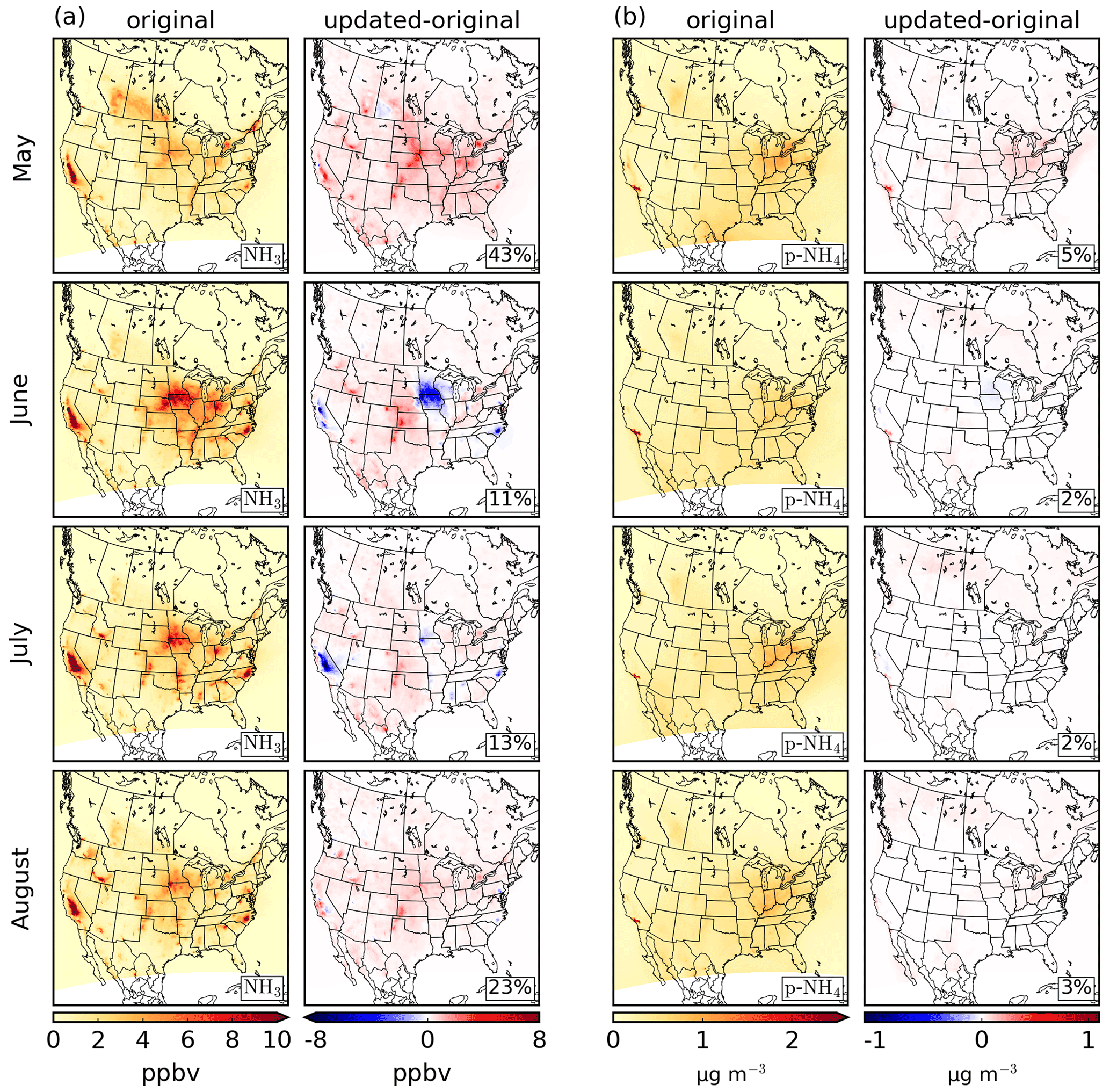
Figure 5 Monthly mean surface (a) NH₃ VMR and (b) p-NH₄ concentration fields from GEM-MACH for May to August 2016. In panels (a) and (b), the left columns show the mean surface field when the original ammonia emissions are used, and the right columns show the mean difference between the GEM-MACH runs with the updated ammonia emissions from the inversion and the original emissions. For plots in the right columns, the total difference over the model domain as a percentage of the original field is shown in the lower right corner. Plots for p-NH₄ show the total ammonium mass over both aerosol size bins.

As with the emissions, when the updated emissions are used the most significant changes in the ammonia surface VMR field occur in the central US, California, and the Canadian prairie provinces. The largest increases in surface ammonia VMR occur in May, where values increase by as much as ∼ 6 ppbv in California's Central Valley and increase by 43 % over the whole domain. Decreases of up to 6–8 ppbv occur in Central California, Minnesota–Iowa, and North Carolina in June and July.

4.1.3 Comparisons with surface observations

Figure 6 shows the NMB values for ammonia observations from the NAPS and AMoN networks. For the moment, we only consider the values for runs that use the original emissions or inversions using the hybrid observation operator, which are displayed with the blue circular markers and red square markers, respectively. These NMB values, as well as the number of observations, NSTD, and correlation coefficient, are shown in Table S1. Overall, when the original ammonia emissions are used, GEM-MACH underestimates surface ammonia compared to both the NAPS and AMoN networks. The monthly-mean biases for NAPS and AMoN range from −22.9 % to −46.3 % and −4.2 % to −43.0 %, respectively.

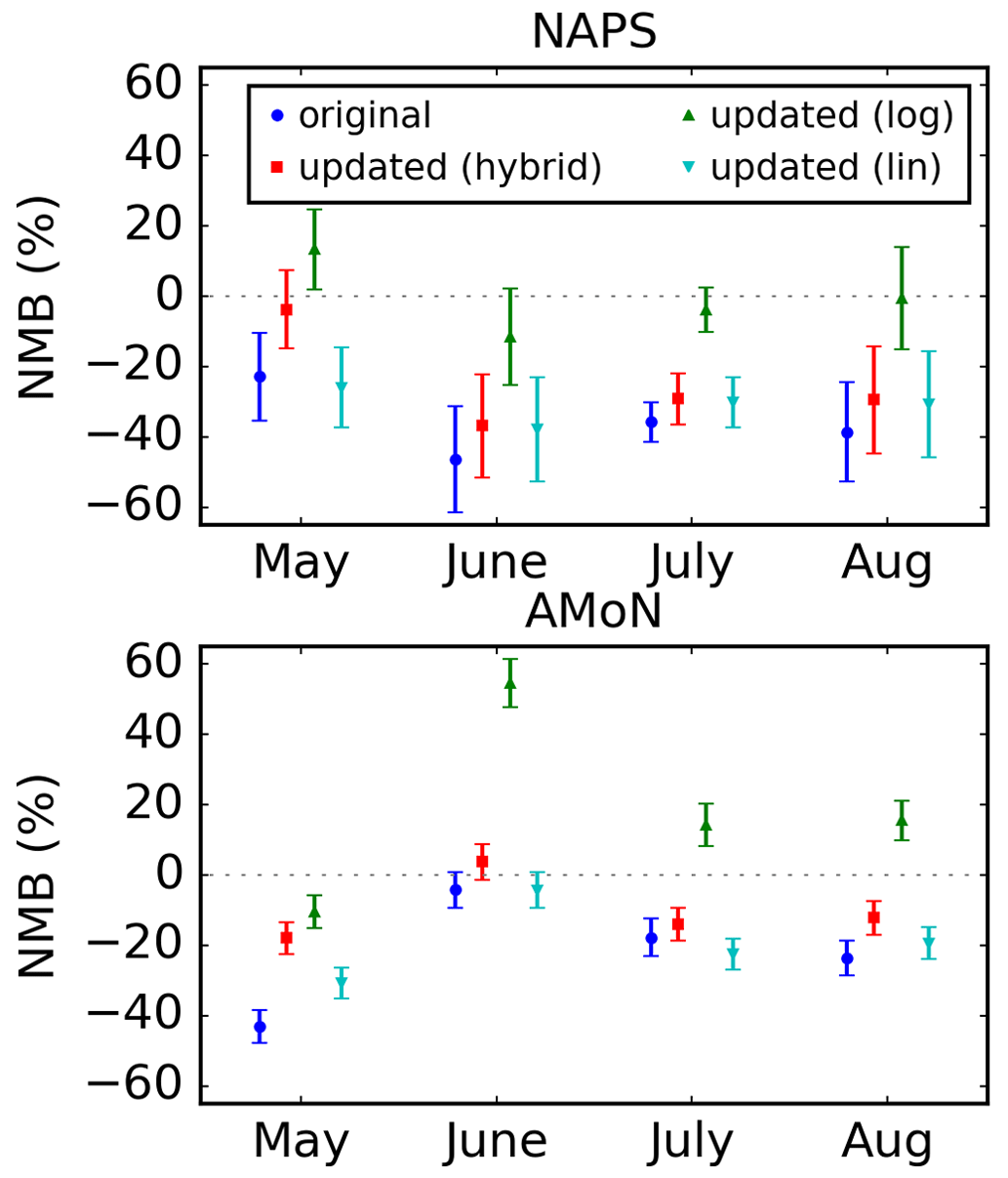
Figure 6 Normalized mean biases between the GEM-MACH ammonia surface fields and observations from the NAPS and AMoN networks for May to August 2016. In the legend, “original” and “updated” indicate the ammonia emissions used in GEM-MACH. The observation operator used in the inversion is indicated in the parentheses of the legend labels. Error bars denote the standard error.

Comparing the NMB values between the original and updated emissions cases, we see that using the ammonia emissions from the inversions that utilize the hybrid observation operator reduces the underestimation in GEM-MACH in every month for both networks, although not completely eliminating it in most cases. The largest reductions in NMB for both observation networks occur in May, where the NMB is reduced by 19.1 % and 25.1 % (percentage points) for NAPS and AMoN, respectively. The reduction in bias is closer to 5 %–10 % for June to August for both networks. We note that while the bias is reduced in all cases examined, some of the reductions in bias have lower statistical significance, such as for NAPS in June (see Table S1 in the Supplement).

The normalized standard deviation of differences and correlation coefficients for the surface ammonia observations are shown in Table S1. From this table, we can see that while the standard deviation of differences decrease in most cases when the updated ammonia emissions are used (with NAPS in July and August being the exception), in all cases these changes have relatively low statistical significance. The correlation coefficients between GEM-MACH and the ammonia surface observations increase for all months for AMoN but decrease for NAPS for the months of June, July, and August, although the difference for June has low statistical significance.

Figure 7 shows statistics for the individual stations measuring surface ammonia. The left and middle columns of this figure show the bias when the original and updated emissions are used, respectively, while the improvement at each station as measured by the root-mean-square error (RMSE) is shown in the right column. We can see that when the original emissions are used, GEM-MACH persistently underestimates ammonia in some regions, such as in Utah, Colorado, and Wyoming, where all stations have negative biases over all months. However, for other regions, most notably in Illinois, Wisconsin, and Indiana, the biases in the GEM-MACH surface ammonia fields switch between positive and negative depending on the month. Although some stations do show overestimations, in each month the majority of stations show underestimations of the GEM-MACH surface ammonia when the original emissions are used.

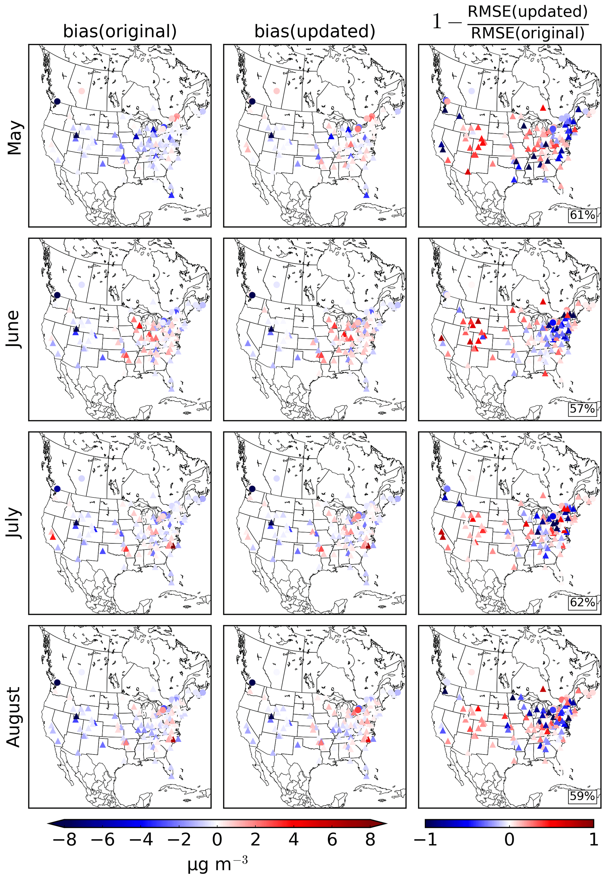
Figure 7 Comparison of ammonia surface observations from the NAPS and AMoN networks with GEM-MACH surface fields. The left and center columns show bias values for each station when the original and updated ammonia emissions are used, respectively. The right column shows the relative improvement of the root-mean-square error (RMSE) for each station. NAPS and AMoN stations are denoted with circular and triangular markers, respectively. For the plots in the right column, the percentage of stations that have a lower RMSE value when the updated ammonia emissions are used is shown in the lower right corner.

The bias values of a majority of stations in the central US improve when the updated emissions are used. However, a few clusters of stations near the US east coast have higher biases when the emissions from the inversions are used. In this data set, only one station is located in one of the regions that showed a significant drop in emissions (Minnesota–Iowa, North Carolina, the Central Valley, southern Saskatchewan), which is located in Clinton, North Carolina. Observations from this station, which were only available in July and August, showed an over-prediction of ammonia for both of these months when the original emissions were used, as Battye et al. (2019) also found for this location. Using the emissions from the inversions decreased the over-predictions at the Clinton station by 3.89 and 1.80 µg m⁻³ in July and August, respectively.

4.1.4 Observation operator selection

In Sect. 3.3, it was shown that the particular observation operator used for the model–retrieval comparison may have a significant impact on the emissions inversion. Figure 8 shows a comparison of the ammonia emissions increments that result from inversions that use the different observation operators described in Sect. 3.3. The increments shown in the middle and right columns of Fig. 8 were the result of inversions in which all retrievals were compared to GEM-MACH using only the log-space or linear-space observation operators, respectively, while the left column shows the increment using the hybrid method (identical to that in Fig. 3, shown for comparison).

The discussion in Sect. 3.3 suggested that if the log-space observation operator is used for the model comparison for all retrievals, the ammonia increment may be overestimated due to the “zeroing out” of some model profiles. On the other hand, using the linear-space observation operator in all cases tends to overestimate the GEM-MACH analogue profile, thereby underestimating the increment. This general behaviour is evident in the increments shown in Fig. 8, where the inversions that use the log-space (linear-space) observation operator for all comparisons yield increments that are larger (smaller) than the increment from the hybrid operator in many locations. This is particularly notable in southern Saskatchewan in May and southern Minnesota and Iowa in June, where emissions were removed when the hybrid operator was used but had emissions added when the log-space operator was used instead. In contrast, when the linear-space observation operator was used, these regions had more emissions removed over a larger area. The largest differences between emissions increments occur in June, where the increment produced using the log-space observation operator in the midwestern US and California is significantly larger than that produced using the hybrid and linear-space operators.

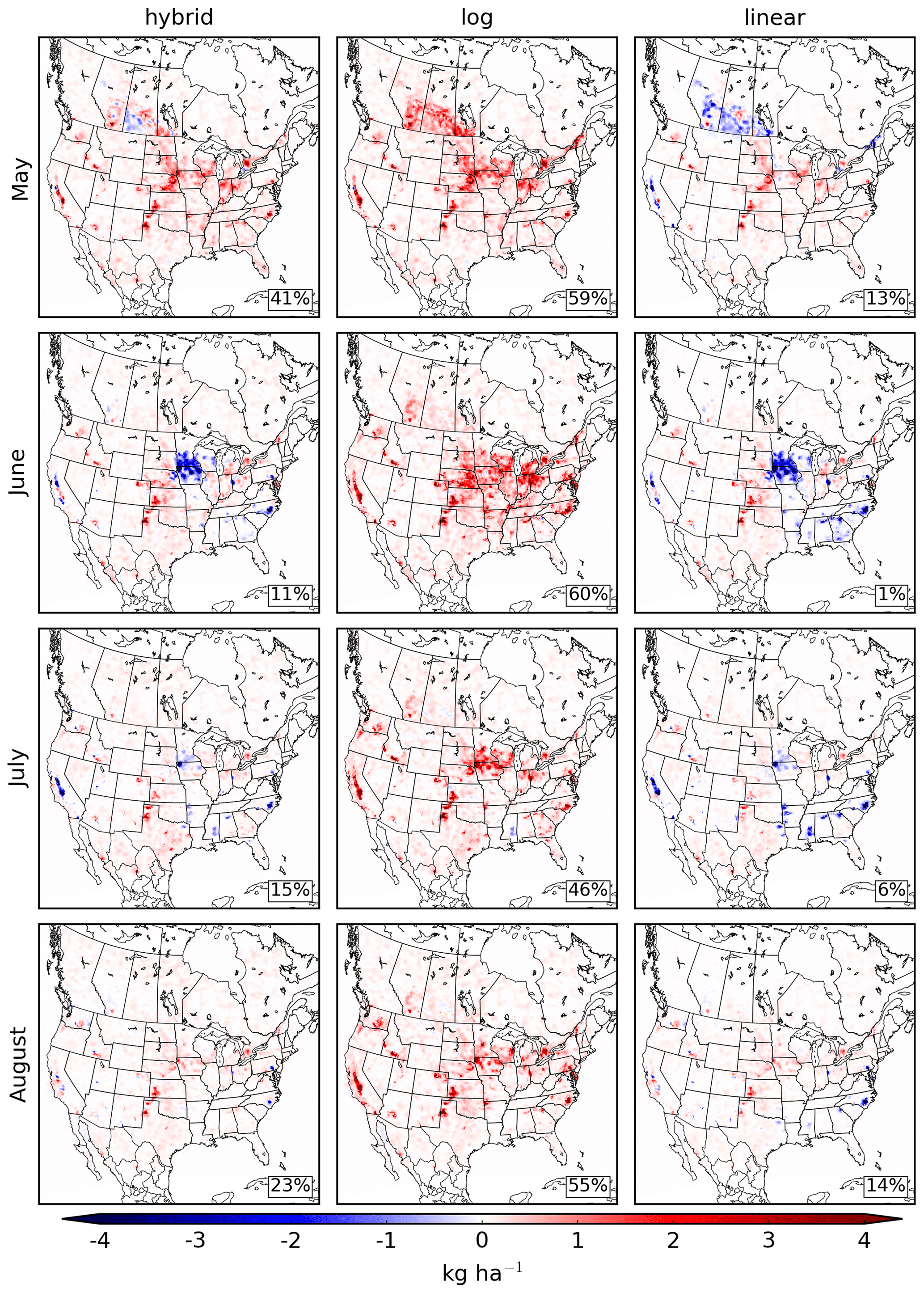
Figure 8 Monthly mean ammonia emissions increments for May to August 2016 for inversions using different observation operators. Inversions displayed in the left, middle, and right columns use the hybrid, log, and linear observation operators, respectively. The left column, which is identical to the right column of Fig. 3, is shown for comparison. Percentages in the lower right corners show the change over the whole domain.

Returning to Fig. 6, we can see that the choice of observation operator has a similar effect on the comparisons with ammonia surface observations. For the comparisons with the AMoN network, using the log-space operator raises the biases compared to the values using the hybrid observation operator, while using the linear-space observation operator lowers these values. The same is true of NAPS for the month of May. However, for NAPS in June to August, there is little difference between the hybrid and linear-space operators since the hybrid method selects the linear-space operator the majority of the time in these months at the NAPS locations (seen by comparing Figs. S2 and S8). In May, the hybrid method selects the log-space operator most often at the NAPS and AMoN locations, resulting in larger differences between the hybrid and linear methods, where the NAPS and AMoN biases are about 23 % and 13 % more negative, respectively, when the linear-space operator is used instead of the hybrid operator. Comparing the absolute NMB values of the linear-space and hybrid observation operators, the hybrid operator yields smaller or equal values in all cases.

Comparing the hybrid and log-space operators in Fig. 6, we can see that the method with the best performance as judged by the NMB changes with the month and network. The hybrid method yields the lowest bias for NAPS in May and for AMoN in June, July, and August, while the log-space method gives the lowest values for the remaining cases. The differences between the hybrid and log-space operators are generally larger in June to August compared to May, as the hybrid method selects the log-space operator for the majority of retrievals in May, in contrast to June to August where the log-space operator is selected less often. As noted above, the largest differences between the emissions increments produced using the hybrid and log-space observation operators occur in June in the midwestern US and in California, where the log-space increment is significantly larger in these areas than for the hybrid increment. The impact of this large increment can be seen in Fig. 6, where large overestimations of the GEM-MACH ammonia surface fields are seen in June for AMoN when the log-space operator is used in the inversion. The NMB is much larger for this case than for any other months and network, including cases that used the original ammonia emissions.

Overall, using the hybrid observation operator for the comparison of GEM-MACH to the CrIS retrievals in the inversion generally yields favourable results when evaluating the inversions using NAPS and AMoN observations. While using the log-space operator yields good results for many cases, the large overestimation of ammonia emissions in some places in the US in June demonstrates that this operator must be used with caution. For the remainder of this paper, all results shown will be for inversions that use the hybrid operator.

4.2 Impact on PM formation

As ammonia plays an important role in inorganic PM formation, we now examine what impact, if any, the ammonia emissions inversions have on species related to inorganic PM in GEM-MACH.

4.2.1 Predicted PM profiles

To illustrate the process of PM formation in GEM-MACH, Fig. 9 shows the mean profiles for p-NH₄, p-NO₃, and p-SO₄ and the precursor gases NH₃, HNO₃, and SO₂ for May 2016 at two different locations. The panels on the left show the monthly mean profiles of GEM-MACH run with the original ammonia emissions, while the panels on the right show the mean differences between GEM-MACH run with the updated and original ammonia emissions. The upper and lower panels show the profiles near Toronto, Ontario, and the city of Grand Junction in western Colorado, respectively. The profiles for p-NH₄, p-NO₃, and p-SO₄ are computed by taking the sum of the fine and coarse aerosol bins of each species.

As the inversion increased the ammonia emissions in both locations shown in Fig. 9, the ammonia difference profiles shown in the right panels are positive for both locations, peaking at the surface and decreasing with height. Figure 9 shows little change in SO₂ or p-SO₄. The oxidation of S(IV) to S(VI) is primarily controlled by the aqueous-phase oxidation of S(IV) with ozone, hydrogen peroxide, and organic peroxides (Seinfeld and Pandis, 2006). While the S(IV) oxidation rate is sensitive to pH, and thus may be sensitive to ammonia levels, in these locations this effect is small. Furthermore, since the formation of inorganic PM through reactions such as 2${\mathrm{NH}}_{\mathrm{4}}^{+}\left(\mathrm{aq}\right)$ + ${\mathrm{SO}}_{\mathrm{4}}^{\mathrm{2}-}\left(\mathrm{aq}\right)$ ⇌ (NH₄)₂SO₄(s) does not change the total amount of sulfate, the total sulfate profile shows little change when the emissions from the inversions are used.

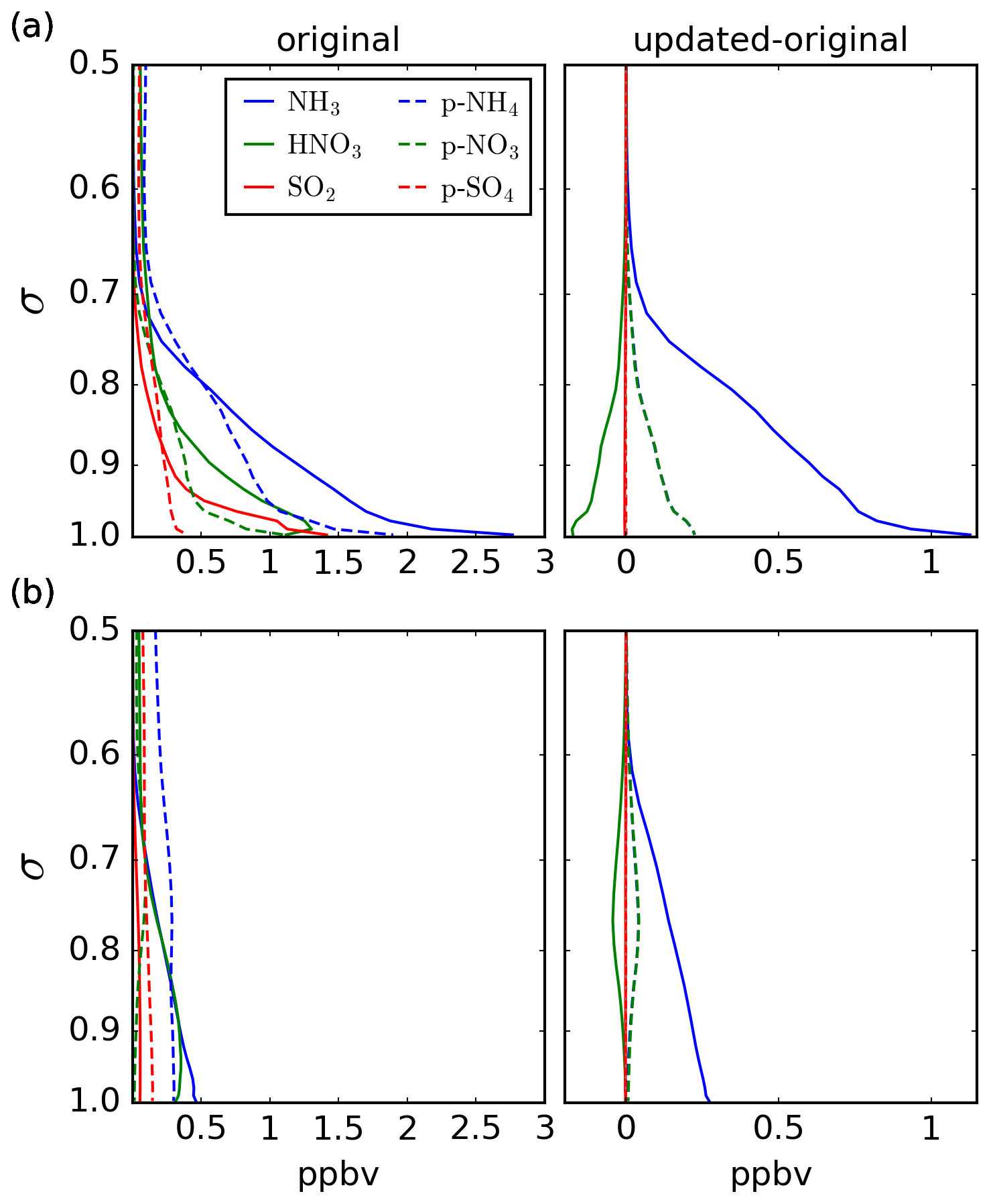
Figure 9 Monthly mean vertical profiles near (a) Toronto, Ontario, and (b) Grand Junction, Colorado, for May 2016. Plots on the left show mean profiles for GEM-MACH run with the original ammonia emissions, while plots on the right show mean differences between the updated and original runs. The vertical coordinate σ is the ratio of the pressure to the surface pressure. The legend in the upper left plot applies to all plots.

As ammonia preferentially neutralizes sulfate over nitrate, significant nitrate formation through the reaction NH₃(g) + HNO₃(g) ⇌ NH₄NO₃(s) will only occur if ammonia levels exceed the amount needed to neutralize the sulfates. For the profile near Toronto, the amount of ammonia close to the surface exceeds that required for sulfate neutralization, and so a non-negligible amount of nitrate formation can occur near the surface. This can been seen in the upper right panel of Fig. 9, which shows a decrease in HNO₃ that peaks at the surface and lessens with height, which is mirrored by increases in p-NO₃ and p-NH₄. In contrast, for the location in western Colorado shown in the lower panels of Fig. 9, at the surface ammonia levels are only high enough for sulfate neutralization, having a ratio of surface NH_x (ammonia gas + ammonium aerosol) to sulfate of roughly half of that for the location near Toronto. Consequently, little nitrate formation occurs at the surface for the location in western Colorado. However, as the NH_x-to-sulfate ratio increases with altitude at the western Colorado location, ammonium nitrate formation occurs at higher altitudes, as seen in the lower right panel of Fig. 9. As such, unlike the changes in ammonia, the largest changes in ammonium nitrate concentrations may or may not occur near the surface.

4.2.2 Impacts of inversions on predicted PM fields

The monthly mean differences in the GEM-MACH surface fields for p-NH₄, HNO₃, and p-NO₃ when the updated ammonia emissions are used are shown in Figs. 5b and 10. As seen in Fig. 10, areas with increased ammonia emissions have depleted levels of HNO₃ and increased levels of p-NO₃ due to increased neutralization with ammonia. As ammonia emissions increased in the majority of areas in the model domain, HNO₃ decreased and p-NO₃ increased in most regions. In southern California and the midwestern US, the monthly mean surface p-NO₃ levels increased by as much as ∼ 2 µg m⁻³. The largest increases in surface nitrate occurred in May, increasing by 28 % over the whole domain. Note that the regions with the largest increases in p-NH₄ and p-NO₃ do not necessarily coincide with the regions with the largest increases in ammonia emissions, as the spatial distribution of HNO₃ can have a large impact on the spatial distribution of ammonium nitrate.

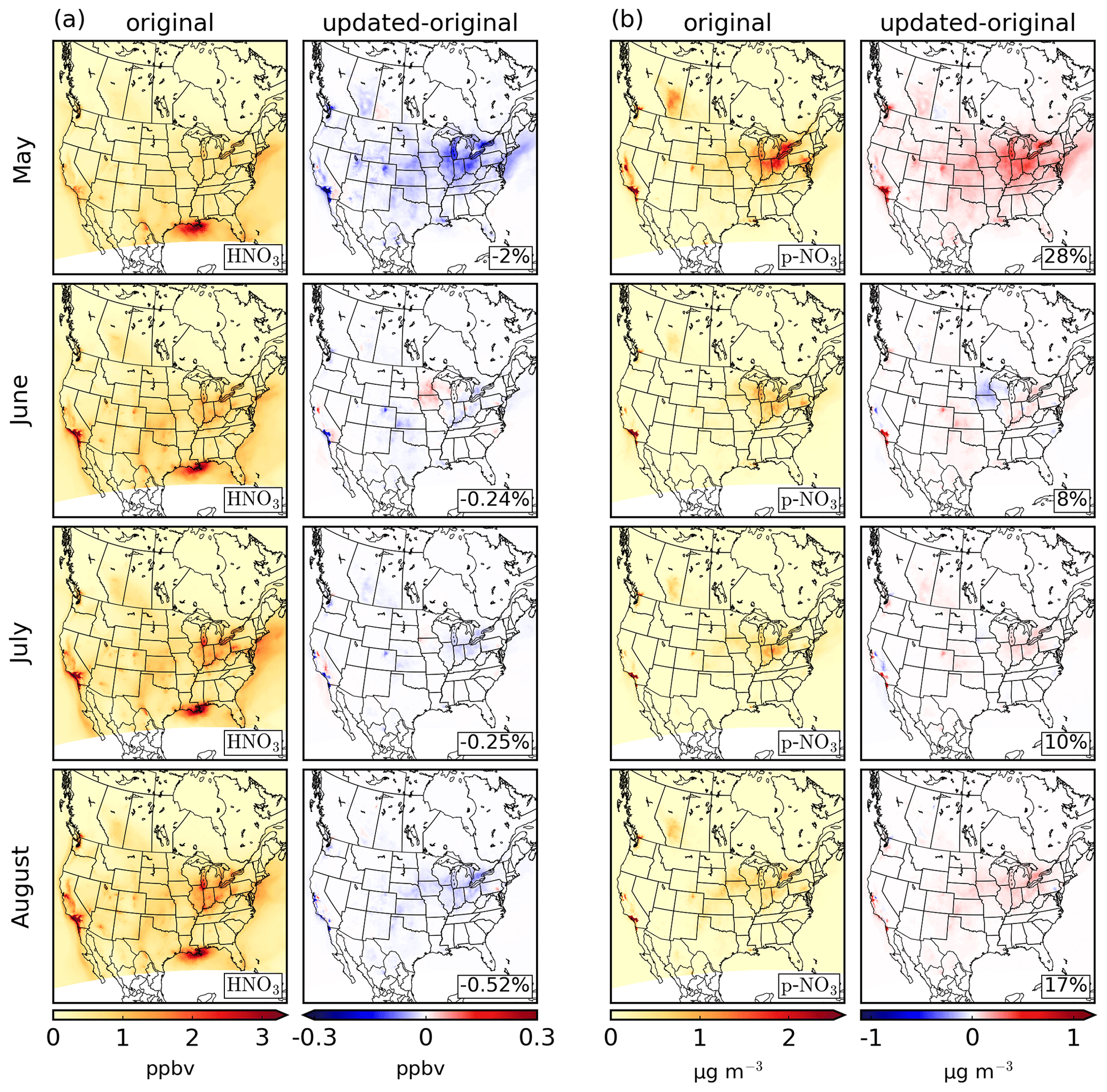
Figure 10 Same as Fig. 5, except for (a) HNO₃ and (b) p-NO₃.

The mean differences in the surface SO₂ and p-SO₄ GEM-MACH fields are shown in Fig. S3. The mean differences of the surface SO₂ and p-SO₄ fields range from −0.062 to 0.007 ppbv and from −0.032 to 0.158 µg m⁻³, respectively. As previously noted by Makar et al. (2009) and noted above, these changes are in part due to changes in the aqueous-phase oxidation rates of S(IV) to S(VI) caused by changes in pH, in addition to changes in the PM dry deposition rates due to changes in the aerosol size distribution.

4.2.3 Comparisons with surface observations

Figure 11 shows the NMB values for HNO₃, p-NH₄, and p-NO₃ observations from the CAPMoN and CASTNET networks for the GEM-MACH runs with the original ammonia emissions and the emissions from the inversions. Statistics for these species, as well as for SO₂ and p-SO₄, are also given in Tables S1–S3. In addition, statistics for individual stations are shown in Figs. S4–S7. As seen in Fig. 11, when the original ammonia emissions are used, GEM-MACH over-predicts surface HNO₃ and under-predicts p-NH₄ and p-NO₃. These over- and under-predictions are seen at almost every station (see Figs. S4–S7). The magnitude of the CAPMoN NMB values for HNO₃, as well as the CASTNET NMB values for HNO₃ in August, are in general larger than the magnitudes of the NMB values for p-NH₄ and p-NO₃, with the HNO₃ NMB value reaching as high as ∼ 170 % for CAPMoN in August. The biases for all p-NH₄ and p-NO₃ cases, as well as CASTNET HNO₃ for May to July and CAPMoN HNO₃ for May, are within 100 %. When the ammonia emissions from the inversions are used, ammonium nitrate production increases in most locations within the model domain, resulting in decreases in the overestimations of HNO₃ and in the underestimations of p-NH₄ and p-NO₃. This improvement is most notable in May, where the p-NH₄ and p-NO₃ biases improve by ∼ 5 % and ∼ 10 %–13 %, respectively. While the NMB values for HNO₃ are reduced when the updated ammonia emissions are used, these reductions have low statistical significance for most cases and are relatively small compared to the overall size of these biases which range between 50 % and 170 %. The overestimation in HNO₃ will be discussed further in Sect. 4.3. As the changes in the SO₂ and p-SO₄ surface fields were small, the change in the biases of the corresponding observations were small as well (see Table S3).

Although using the updated ammonia emissions increased the NSTD values for HNO₃, p-NH₄, and p-NO₃ in some cases, in all cases the change in NSTD had low statistical significance (see Tables S1 and S2). Likewise, the changes in correlation coefficients for these observations had relatively low statistical significance (with the possible exception of CAPMoN p-NH₄ in May).

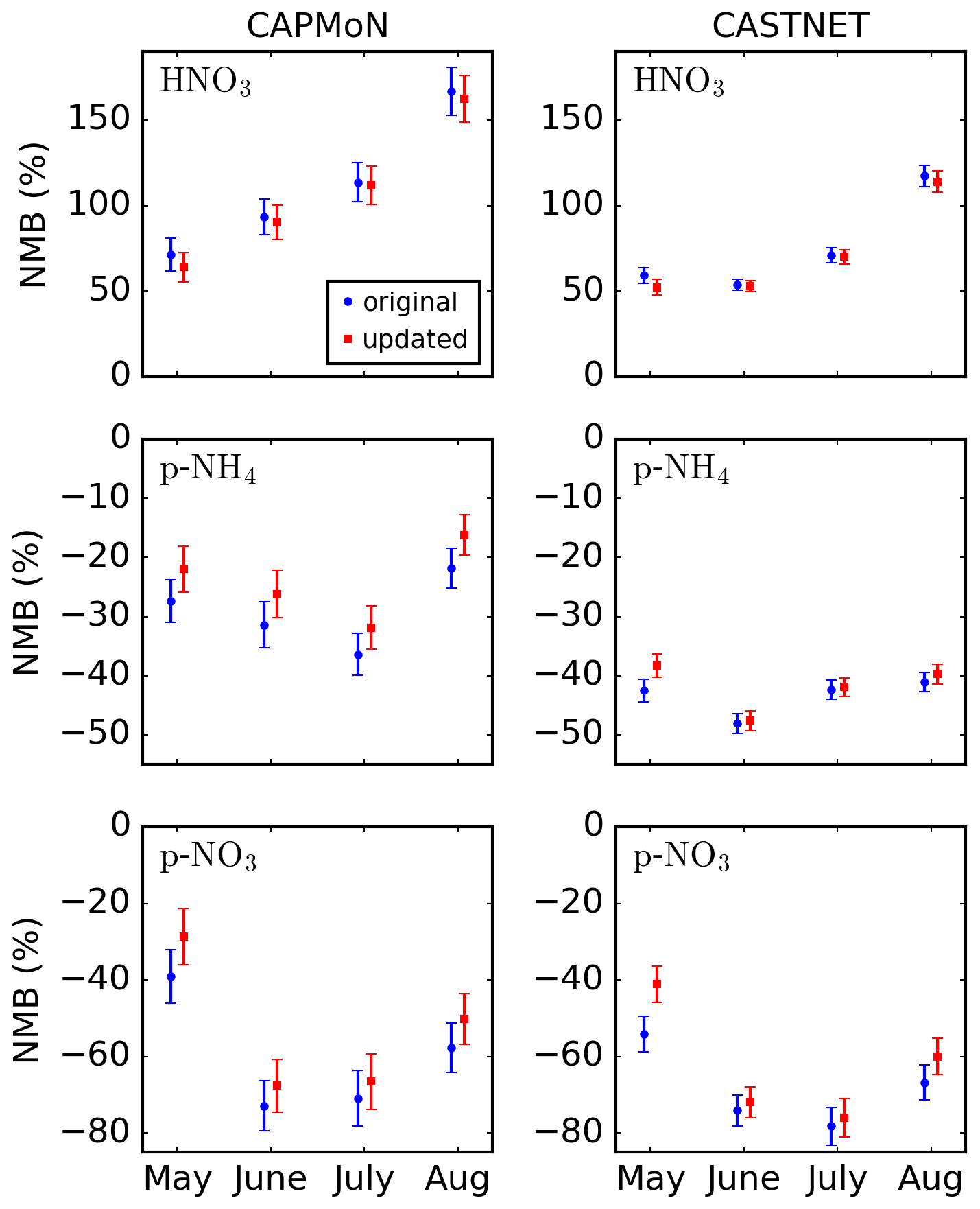
Figure 11 Normalized mean biases between GEM-MACH HNO₃, p-NH₄, and p-NO₃ surface fields and observations from the CAPMoN and CASTNET networks for May to August 2016. In the legend, “original” and “updated” indicate the ammonia emissions used in GEM-MACH. Error bars correspond to the standard error.

Both CAPMoN and CASTNET employ a three-stage filter pack consisting of, in series, a Teflon filter to collect p-NH₄, p-NO₃, and p-SO₄, followed by a nylon filter to collect HNO₃ (and some SO₂), and finally cellulose filters impregnated with K₂CO₃ to collect the remaining SO₂ (see Table 1). The volatilization of ammonium nitrate on Teflon filters can be significant (Hering and Cass, 1999; Ashbaugh and Eldred, 2004), especially during warm months. For these types of filter packs, the volatilization of aerosol ammonium nitrate to gaseous NH₃ and HNO₃ on the Teflon filter and the subsequent collection of HNO₃ on the nylon filter can cause an underestimation of nitrate and overestimation of HNO₃ (Sickles and Shadwick, 2002, 2007, 2015). Accounting for this effect would make the biases shown in Fig. 11 larger, but the decrease in the (unnormalized) biases when using the emissions from the inversion would remain the same. In contrast, coarse particles collected on the Teflon filter may scavenge HNO₃, which would create a high nitrate bias and a low HNO₃ bias (Sickles and Shadwick, 2007, 2015).

4.3 Impact on PM size distribution

4.3.1 Impact of inversions on the PM size distribution

The previous section examined the impact of the ammonia emissions inversions on the total amount of ammonium, nitrate, and sulfate. In this section, we explore the impact of the emissions inversions on the size distribution of inorganic PM, and we focus on the impact on PM_2.5 in particular due to its significance in air quality. As mentioned in Sect. 2.3, GEM-MACH first uses the HETV package to determine the gas–particle partitioning of inorganic species using a bulk approach, followed by the partitioning of the PM into size-resolved bins. As such, much of the focus of this section will be on the partitioning into size bins following the bulk calculation. In the previous section, it was shown that using the ammonia emissions from the inversions increased ammonium nitrate production in most locations within the model domain (with a few notable exceptions mentioned in previous sections). While significant amounts of nitrate can be found in both fine and coarse particles, ammonium nitrate production is usually associated with fine particles, whereas the nitrate found in coarse particles more often results from reactions between HNO₃ and crustal materials (calcium, potassium, magnesium) or sodium chloride (Seinfeld and Pandis, 2006).

Figure 12 shows the monthly mean change in the fine- (PM_2.5) and coarse-fraction (PM_2.5−10) ammonium and nitrate GEM-MACH fields when the ammonia emissions from the inversions are used. One of the most notable features of these plots is the large amounts of ammonium and nitrate being added to the coarse-fraction bin. This is particularly notable for ammonium, where for many locations where total ammonium increases (see Fig. 5), the amount of mass added to the coarse-fraction bin is larger than that added to the fine bin, and in some locations the mass in the fine bin actually decreases.

GEM-MACH uses a quasistationary bin-size structure (Jacobson, 1997), where particle volumes are initially allowed to grow or shrink but are then fit back into a stationary bin structure following the change in particle volume. After the heterogeneous bulk chemistry is run in HETV, almost all of the additional ammonium and nitrate are added to particles in the fine bin. However, due to the use of only two size bins, in many cases the fitting done by the quasistationary structure reallocates large amounts of mass to the coarse-fraction bin, sometimes moving mass from the fine- to the coarse-fraction bin by amounts that exceed the initial amount added to the fine bin. This is a clear limitation of the two-bin model compared to one with a larger number of size bins.

Figure 12 Monthly mean differences of GEM-MACH surface fields for fine- (PM_2.5) and coarse-fraction (PM_2.5−10) ammonium and nitrate for May to August 2016. Plots show mean differences between the run with the updated ammonia emissions and the original emissions. The total difference over the model domain as a percentage of the original field is shown in the lower right corner of each plot.

4.3.2 Comparisons with surface observations

The NMB values between the GEM-MACH PM_2.5-NO₃ and PM_2.5-NH₄ fields and observations from the NAPS, CSN, and IMPROVE networks are shown in Fig. 13. We begin by considering the cases when the original set of emissions are used. In contrast to p-NH₄ and p-NO₃ that were underestimated by GEM-MACH compared to CAPMoN and CASTNET (Fig. 11), PM_2.5-NH₄ and PM_2.5-NO₃ are overestimated for NAPS and CSN. The relative magnitude of the overestimations of PM_2.5-NH₄ and PM_2.5-NO₃ for NAPS and CSN are much larger than the magnitude of the underestimations of p-NH₄ and p-NO₃, with a number of the PM_2.5-NH₄ and PM_2.5-NO₃ NMB values exceeding 100 %. On the other hand, the NMB values for PM_2.5-NO₃ from IMPROVE have significantly smaller absolute values, and GEM-MACH underestimates the fields in many cases.

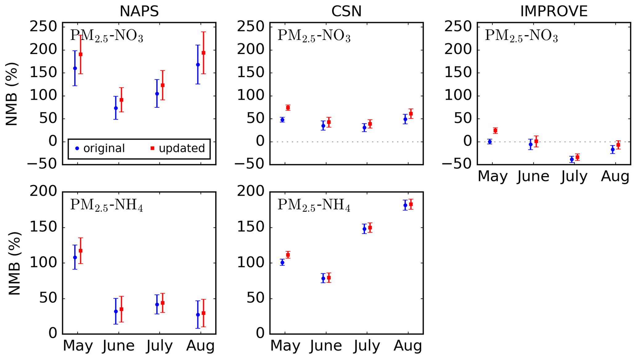
Figure 13 Monthly normalized mean biases between GEM-MACH PM_2.5-NO₃ and PM_2.5-NH₄ surface concentration fields and observations from the NAPS, CSN, and IMPROVE networks for May to August 2016. In the legend, “original” and “updated” indicate the ammonia emissions used in GEM-MACH. Error bars correspond to the standard error.

Now turning our attention to the impact of the emissions inversions on the biases, we can see that in most cases using the emissions from the inversions degrades the NMB values, though for many cases the size of this degradation is much smaller than the magnitude of the overall bias. Furthermore, if less mass was transferred from the fine to the coarse ammonium and nitrate bins during the quasistationary fitting procedure, then the biases for NAPS and CSN PM_2.5-NH₄ and PM_2.5-NO₃ would increase further.

Before discussing potential biases in the GEM-MACH model, we consider possible biases in the observations of PM_2.5-NH₄ and PM_2.5-NO₃. For the nylon filters used in the CSN and IMPROVE networks, the nitrate loss from the volatilization of ammonium nitrate was estimated to be minor (Yu et al., 2005b) as the nylon filter can recapture volatilized HNO₃, although loss of ammonium can be significant (Yu et al., 2006). In the NAPS network, nitrate is collected on Teflon filters, on which the volatilization of ammonium nitrate can be significant, as discussed in Sect. 4.2. Some NAPS stations mitigate this nitrate loss through the use of a nylon filter downstream of the Teflon filter that can collect the volatilized HNO₃. For this reason, NAPS stations without the downstream nylon filter were not used in this work.

Many air quality models have been shown to overpredict the concentration of fine nitrate and/or ammonium (although many underpredict fine nitrate in California), often with biases larger in magnitude than biases for sulfate (Yu et al., 2005a; Heald et al., 2012; Walker et al., 2012). While only two PM size bins were used in this work, which very likely plays a significant role in the difficulty predicting fine ammonium and nitrate as noted above, large overpredictions of PM_2.5 ammonium and/or nitrate have also been observed in other models that use significantly more PM size bins (Trump et al., 2015; Zakoura and Pandis, 2018).

Having found similar overestimations of nitric acid and fine nitrate in the GEOS-CHEM model using the ISORROPIA II model (Fountoukis and Nenes, 2007) for the inorganic gas–particle phase partitioning, Heald et al. (2012) found that if the nitric acid levels were artificially lowered by 75 %, then the overprediction of fine nitrate decreases significantly and greatly improved the agreement with PM_2.5-NO₃ observations from the IMPROVE network. A decrease in nitric acid levels of this magnitude would also significantly decrease the high biases in the GEM-MACH nitric acid fields with observations from the CAPMoN and CASTNET networks seen in Fig. 11. However, the mechanism for a decrease of this magnitude was not identified. Heald et al. (2012) and Walker et al. (2012) both showed that significantly reducing the nighttime nitric acid production via the reaction N₂O₅ + H₂O → 2HNO₃ in GEOS-CHEM only yields modest reductions in the PM_2.5-NO₃ bias. Similarly, Heald et al. (2012) found that changes to the oxidation rate of NO₂ by OH, the OH concentration, temperature, and humidity in GEOS-CHEM are unlikely to yield HNO₃ decreases large enough to significantly reduce the PM_2.5-NO₃ biases observed (although these factors may partially explain the PM_2.5-NO₃ biases). Zakoura and Pandis (2018) demonstrated that coarser horizontal grid resolutions may artificially dilute NO_x plumes, resulting in higher N₂O₅, HNO₃, and nitrate levels, although while using finer grid resolutions lessened the overproduction of fine nitrate, significant biases remained.

The competition of ammonia with crustal-material base cations and sea salt for reaction with HNO₃ can significantly impact the size distribution of nitrate. Reactions of HNO₃ with crustal materials and sea salt are currently not implemented in HETV. While including these reactions in HETV may significantly change the nitrate size distribution, the overprediction of fine nitrate has been shown to persist in models using ISORROPIA II, which includes these reactions (Walker et al., 2012; Trump et al., 2015). Trump et al. (2015) demonstrated that heterogeneous partitioning models that are based on the assumption of thermodynamic equilibrium, such as ISORROPIA II (and HETV), may not accurately represent the interactions between nitric acid and coarse particles and that using an explicit mass transfer approach for these interactions can shift nitrate from the fine to the coarse mode in locations with significant amounts of sea salt or dust.

Figure 14 shows the NMB values for total PM_2.5 for observations from NAPS and AQS networks for BAM and TEOM instruments. The total PM_2.5 is underestimated by GEM-MACH, with NMB values in the range of −60 % to −2 %. Although PM_2.5-NH₄ is overestimated, and PM_2.5-NO₃ is overestimated for the CSN and NAPS networks (Fig. 13), large underestimations of fine organic PM (Stroud et al., 2011) counteract the overestimations in fine inorganic PM. Only small changes are seen in the total PM_2.5 biases when the emissions from the inversions are used. This is in part due to many locations where GEM-MACH predicts increases in PM_2.5-NO₃ and also predicts decreases in PM_2.5-NH₄.

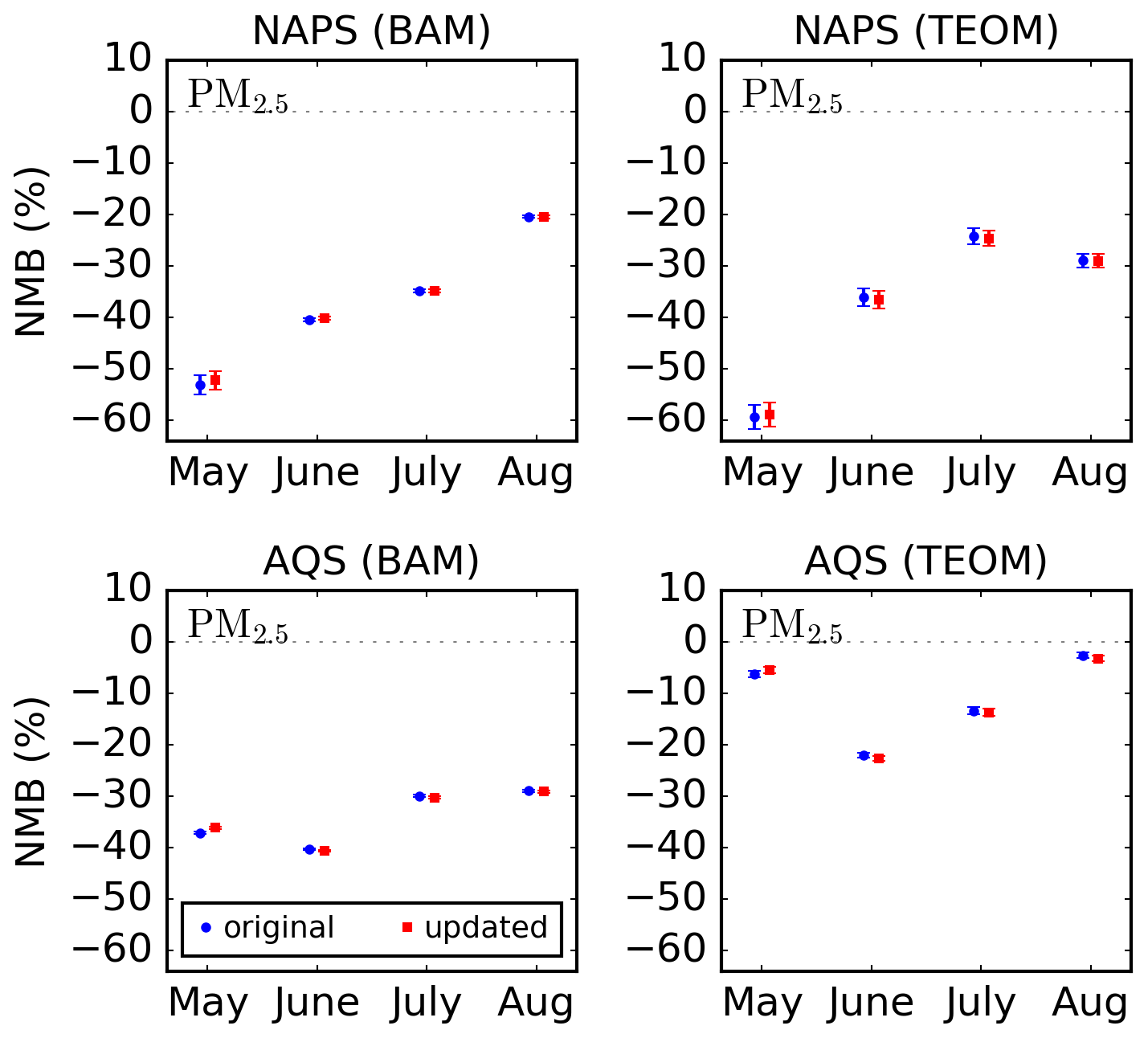
Figure 14 Normalized mean biases between GEM-MACH total PM_2.5 surface fields and BAM and TEOM observations from the NAPS network and observations reported to the AQS for May to August 2016. In the legend, “original” and “updated” indicate the ammonia emissions used in GEM-MACH. Error bars correspond to the standard error.

4.4 Impact on deposition

The previous sections showed that using the ammonia emissions from the inversions led to non-negligible changes in the levels of ammonia, ammonium, and nitrate ambient concentrations. In this section, we examine the changes in the removal of these species through deposition. Figure 15 shows the spatial distribution of monthly changes in the total (dry + wet) deposition rates of NH_x and HNO₃ + NO₃. The changes in NH_x deposition closely resembles the changes in the surface fields shown in Fig. 5. The largest increases in deposition were in May, where NH_x total deposition increased by as much as 3.7 × 10⁻⁴ $\mathrm{mol}{\mathrm{m}}^{-\mathrm{2}}{\mathrm{d}}^{-\mathrm{1}}$. The largest decreases in deposition were in the Minnesota–Iowa region in June, where deposition dropped by as much as 3.4 × 10⁻⁴ $\mathrm{mol}{\mathrm{m}}^{-\mathrm{2}}{\mathrm{d}}^{-\mathrm{1}}$. The changes in HNO₃ + NO₃ deposition are an order of magnitude less than the changes in NH_x deposition. While the changes in ammonium and nitrate were similar in magnitude, the changes in NH₃ were much higher than the changes in HNO₃, leading to much larger changes in the amount of NH₃ scavenged by precipitation compared to HNO₃. As with NH_x, the largest increases in HNO₃ + NO₃ deposition occurred in May, but only increased by as much as 0.53 × 10⁻⁴ $\mathrm{mol}{\mathrm{m}}^{-\mathrm{2}}{\mathrm{d}}^{-\mathrm{1}}$.

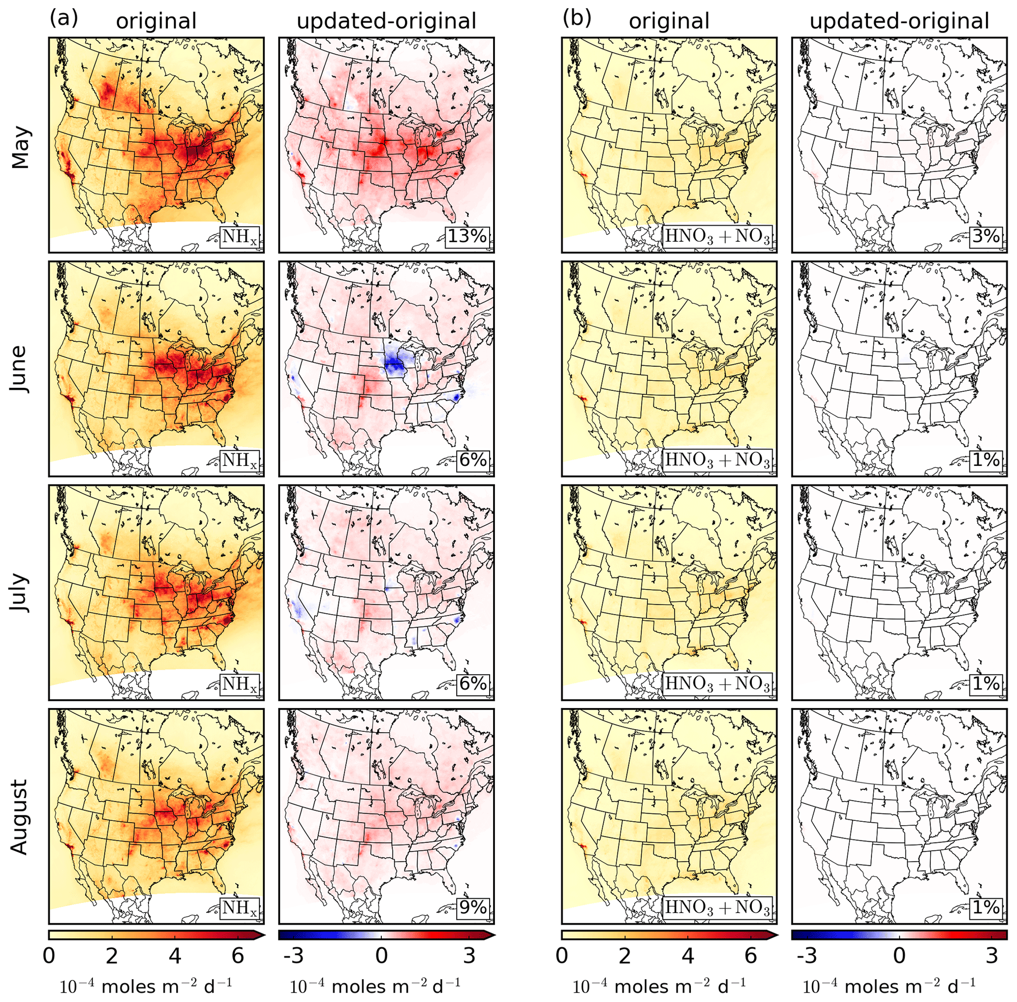
Figure 15 Same as Fig. 5, except for the total (dry + wet) deposition rates of (a) NH_x and (b) HNO₃ + NO₃.

Figure 16 shows the NMB values for ammonium precipitation observations from the CAPMoN, NTN, and AIRMoN precipitation–chemistry networks. The full set of statistical measures for the precipitation–chemistry observations are given in Tables S4 and S5, and statistics for each station for the ammonium precipitation observations are shown in Fig. S7. From Fig. 16, we can see that GEM-MACH under-predicts ammonium wet deposition in all cases, with NMB values ranging between −80 % and −50 %. As with the under-prediction of p-NH₄, the under-prediction of ammonium wet deposition is seen at almost every station (see Fig. S7). Using the updated ammonia emissions reduced these biases, with reductions as large as 8 % occurring in May. The reductions for June to August are less statistically significant than the reductions in May. GEM-MACH underestimates nitrate wet deposition as well, although the updated ammonia emissions have little effect on these biases. The changes in NSTD and correlation coefficient generally have low statistical significance, with the possible exception of the correlation coefficient for ammonium NTN in June (see Table S4).

Figure 16 Normalized mean biases of GEM-MACH with original and updated ammonia emissions compared to ammonium precipitation observations from the CAPMoN, NTN, and AIRMoN networks. In the legend, “original” and “updated” indicate the ammonia emissions used in GEM-MACH. Error bars denote the standard error.

5 Conclusions

As ammonia emissions are increasing or staying constant in many parts of North America, in contrast to other pollutants that have decreasing trends, ammonia is increasingly becoming a species of concern. However, current bottom-up ammonia emissions inventories are highly uncertain, especially concerning the spatial and temporal distribution of emissions. Recently developed ammonia retrievals from satellite-borne instruments such as CrIS provide observations of atmospheric ammonia with global coverage. In this study, we developed an ensemble-variational emissions inversion system that utilizes CrIS ammonia retrievals to refine estimates of ammonia emissions that are used in the Canadian GEM-MACH air quality forecasting model. The use of an ensemble allows for the advection, deposition, and chemical reactions of ammonia to be modelled by GEM-MACH within the inversion without requiring an adjoint model. To mitigate the relatively large uncertainties on individual retrievals, each inversion used a month's worth of retrievals to produce new estimates of the monthly mean ammonia emissions on a grid with a horizontal spacing of 0.09^∘ (∼ 10 km).

To investigate the performance of the inversion system, inversions for May to August 2016 were performed, covering some of the months when ammonia levels within the model domain are at their highest. For these months, the CrIS retrievals were larger than the analogous quantities in GEM-MACH for most locations within the model domain, although the opposite was true for some regions such as parts of California, Minnesota, and Iowa in some months. Consequently, the emissions inversions added ammonia emissions in most of the model domain. The largest increases in emissions from the inversions were in May, with emissions increasing by 45.8 % in the contiguous US and by 27.6 % in Canada. The emissions increases in May were largest in the central US, California, and the Canadian Prairies. The largest emissions decreases were in June and July in Minnesota, Iowa, North Carolina, and California. When GEM-MACH was rerun with the ammonia emissions derived from the monthly mean emissions produced by the inversions, the largest changes in the GEM-MACH surface ammonia field occurred in May, where its monthly mean increased by as much as ∼ 7 ppbv in some locations and increased by 43 % over the whole model domain. The inversions also decreased the emissions significantly in some regions for the months of June and July, resulting in decreases by as much as ∼ 9 ppbv in monthly mean surface ammonia in these locations. Using the ammonia emissions produced by the inversions reduced the underestimation of the GEM-MACH ammonia surface field in comparison to observations from the NAPS and AMoN networks, with the largest reductions in NMB occurring in May, where biases were reduced by 19.1 % and 25.1 % for the NAPS and AMoN networks, respectively.

A novel hybrid approach for comparing logarithmic retrieval parameters to a model profile in an inversion was developed that attempts to pick the best method of comparison between utilizing the averaging kernel in log-space or linear-space depending on the situation. Inversions that used the log-space (linear-space) averaging kernel for all comparisons produced emissions increments that were significantly more positive (negative) compared to the increments produced using the hybrid method. When comparing the resulting GEM-MACH ammonia surface fields to observations from the NAPS and AMoN networks, the hybrid comparison method yielded smaller or equal biases than when using the linear-space operator. For some months/networks, using the log-space operator for all comparisons yielded biases lower in magnitude than that produced using the hybrid method. However, using the log-space operator also yielded the largest NMB value for all cases examined, at just under 60 %. Overall, the hybrid method developed in this work was effective in reducing the biases between GEM-MACH and the ammonia surface observations.

The ammonia emissions inversions increased ammonium nitrate production in GEM-MACH over much of the model domain. The largest increases occurred in May, where surface nitrate increased by 28 % over the model domain. In some regions, such as southern California and the midwestern US, the monthly mean surface nitrate increased by as much as 2 µg m⁻³. Using the original set of ammonia emissions, GEM-MACH over-predicted HNO₃ and under-predicted p-NH₄ and p-NO₃ compared to observations from the CAPMoN and CASTNET networks. Using the ammonia emissions from the inversions reduced these over-/under-predictions, although the reductions in the biases of HNO₃ were relatively small compared to the overall bias values. However, significant reductions in the biases of p-NH₄ and p-NO₃ were seen in many cases, most notably for p-NO₃ in May where biases were reduced by 10 %–13 %.

Using the ammonia emissions from the inversions increased NH_x deposition in most regions within the model domain. The change in deposition was greatest in May, where the deposition over the domain increased by 13 %. Using the emissions from the inversions reduced biases with ammonium precipitation observations from the CAPMoN, NTN, and AIRMoN networks, with reductions as large as 8 % in May.

Although using the ammonia emissions from the inversions improved the agreement between surface observations of total ammonium and nitrate, these improvements were not seen when compared to speciated PM_2.5 observations. Using the currently operational version of GEM-MACH, which only has two aerosol size bins, likely played a large part in this result. However, other studies suggest that this may not be the only cause of this result, and other factors such as the interactions of ammonia with crustal materials may need to be accounted for in the heterogeneous chemistry code. Although using the emissions from the inversions degraded the agreement between GEM-MACH and some of the speciated PM_2.5 surface observations, little impact was seen when comparing to total PM_2.5 observations.

This work focused on improving the performance of the currently operational version of GEM-MACH. As the inversions in this study used a whole month's worth of retrievals to yield monthly mean emissions, one potential operational implementation would be to use inversion results for the current month from the year prior. Although this creates a lag of 1 year, lags in operational emissions inventories are typically much larger than a year. Alternatively, an operational implementation could involve inversions being performed periodically with a moving time window using retrievals from the current year to shorten this time lag. However, to properly resolve temporal features in the ammonia signal such as sharp increases due to the application of fertilizer, the inversion time window may have to be reduced, so for example inversions using the last 1–2 weeks worth of data could produce updated emissions for the current week. Although the currently operational version of GEM-MACH does not include a bidirectional flux model for ammonia, the impact of the inversions on a research version of GEM-MACH that includes a bidirectional flux model will be the subject of future work.

Appendix A: Details of the ensemble-variational method for emissions inversions

In this appendix, we review in detail the ensemble-variational method as applied to emissions estimation. We represent the model by an operator ℳ that relates the emissions e to atmospheric concentrations c by $\mathit{c}=\mathcal{M}(\mathit{e},\mathit{\theta })$, where the vector θ represents all model input parameters other than the emissions. If the combined emissions–concentration model state vector x is represented by

$$\begin{array}{}\text{(A1)}& \mathit{x}=\left[\begin{array}{c}\mathit{c}\\ \mathit{e}\end{array}\right],\end{array}$$

then the background error covariance B can be represented in block form as

$$\begin{array}{}\text{(A2)}& \mathbf{B}=\left[\begin{array}{cc}{\mathbf{B}}_{\text{cc}}& {\mathbf{B}}_{\text{ce}}\\ {\mathbf{B}}_{\text{ec}}& {\mathbf{B}}_{\text{ee}}\end{array}\right],\end{array}$$

where ${\mathbf{B}}_{\text{ec}}={\mathbf{B}}_{\text{ce}}^{\mathrm{T}}$. In the expression above, B_cc and B_ee represent the univariate background error covariances for the chemical concentrations and emissions, respectively, while B_ec is their cross-covariance.

By decomposing B_cc as ${\mathbf{B}}_{\text{cc}}={\mathbf{B}}_{\text{cc}}^{\mathrm{1}/\mathrm{2}}{\mathbf{B}}_{\text{cc}}^{\mathrm{T}/\mathrm{2}}$, where ${\mathbf{B}}_{\text{cc}}^{\mathrm{1}/\mathrm{2}}$ is the square root of B_cc, the control vector transform $\mathbf{\Delta }\mathit{c}={\mathbf{B}}_{\text{cc}}^{\mathrm{1}/\mathrm{2}}\mathit{\chi }$ can be defined, so that the cost function in Eq. (2) can be expressed in terms of the control vector χ as

$$\begin{array}{}\text{(A3)}& J\left(\mathit{\chi }\right)={\displaystyle \frac{\mathrm{1}}{\mathrm{2}}}{\mathit{\chi }}^{\mathrm{T}}\mathit{\chi }+{\displaystyle \frac{\mathrm{1}}{\mathrm{2}}}{\left(\mathit{d}-{\mathbf{HB}}_{\text{cc}}^{\mathrm{1}/\mathrm{2}}\mathit{\chi }\right)}^{\mathrm{T}}{\mathbf{R}}^{-\mathrm{1}}\left(\mathit{d}-{\mathbf{HB}}_{\text{cc}}^{\mathrm{1}/\mathrm{2}}\mathit{\chi }\right).\end{array}$$

Assuming that B_ee can similarly be decomposed as ${\mathbf{B}}_{\text{ee}}={\mathbf{B}}_{\text{ee}}^{\mathrm{1}/\mathrm{2}}{\mathbf{B}}_{\text{ee}}^{\mathrm{T}/\mathrm{2}}$ such that ${\mathbf{B}}_{\text{cc}}^{\mathrm{1}/\mathrm{2}}$ and ${\mathbf{B}}_{\text{ee}}^{\mathrm{1}/\mathrm{2}}$ share the same basis, then from Eq. (3) the emissions increment can be found from the transformation $\mathbf{\Delta }\mathit{e}={\mathbf{B}}_{\text{ee}}^{\mathrm{1}/\mathrm{2}}\mathit{\chi }$. In summary, the emissions inversion consists of two steps: first, the cost function in Eq. (A3) is minimized as a function of the control vector χ, followed by using the value of χ found in the minimization in the transform $\mathbf{\Delta }\mathit{e}={\mathbf{B}}_{\text{ee}}^{\mathrm{1}/\mathrm{2}}\mathit{\chi }$ to yield the emissions increment.

To construct background error covariances from an ensemble, we define the ensemble perturbation matrices δC and δE as

$$\begin{array}{}\text{(A4a)}& {\displaystyle }\mathit{\delta }\mathbf{C}={\displaystyle \frac{\mathrm{1}}{\sqrt{K-\mathrm{1}}}}\left[\begin{array}{ccc}\mathit{\delta }{\mathit{c}}_{\mathrm{1}}& \mathrm{\dots }& \mathit{\delta }{\mathit{c}}_K\end{array}\right],\text{(A4b)}& {\displaystyle }\mathit{\delta }\mathbf{E}={\displaystyle \frac{\mathrm{1}}{\sqrt{K-\mathrm{1}}}}\left[\begin{array}{ccc}\mathit{\delta }{\mathit{e}}_{\mathrm{1}}& \mathrm{\dots }& \mathit{\delta }{\mathit{e}}_K\end{array}\right],\end{array}$$

where the vectors δc_i and δe_i are the concentration and emissions perturbations for the ith member of an ensemble of size K. We take these perturbations as

$$\begin{array}{}\text{(A5a)}& {\displaystyle }\mathit{\delta }{\mathit{c}}_i=\mathcal{M}({\mathit{e}}_i,\mathit{\theta })-\mathcal{M}({\mathit{e}}^{\mathrm{b}},\mathit{\theta }),\text{(A5b)}& {\displaystyle }\mathit{\delta }{\mathit{e}}_i={\mathit{e}}_i-{\mathit{e}}^{\mathrm{b}},\end{array}$$

where e^b are the background (i.e. original) emissions. This is the formulation of 4DEnVar (using the nomenclature of Bannister, 2017) but constructs the ensemble perturbations by subtracting the background instead of the ensemble mean. A localization matrix L is applied to the ensemble perturbations, which can be written in block form as

$$\begin{array}{}\text{(A6)}& \mathbf{L}=\left[\begin{array}{cc}{\mathbf{L}}_{\text{cc}}& {\mathbf{L}}_{\text{ce}}\\ {\mathbf{L}}_{\text{ec}}& {\mathbf{L}}_{\text{ee}}\end{array}\right],\end{array}$$

where ${\mathbf{L}}_{\text{ec}}={\mathbf{L}}_{\text{ce}}^{\mathrm{T}}$. The ensemble-based background error covariance is then constructed as

$$\begin{array}{}\text{(A7)}& \mathbf{B}=\left[\begin{array}{cc}{\mathbf{L}}_{\text{cc}}\circ \left(\mathit{\delta }\mathbf{C}\mathit{\delta }{\mathbf{C}}^{\mathrm{T}}\right)& {\mathbf{L}}_{\text{ce}}\circ \left(\mathit{\delta }\mathbf{C}\mathit{\delta }{\mathbf{E}}^{\mathrm{T}}\right)\\ {\mathbf{L}}_{\text{ec}}\circ \left(\mathit{\delta }\mathbf{E}\mathit{\delta }{\mathbf{C}}^{\mathrm{T}}\right)& {\mathbf{L}}_{\text{ee}}\circ \left(\mathit{\delta }\mathbf{E}\mathit{\delta }{\mathbf{E}}^{\mathrm{T}}\right)\end{array}\right],\end{array}$$

where ∘ is the Hadamard (element-wise) product. The square roots of the background error covariances, which are used in the cost function given in Eq. (A3) and the emissions control vector transform, can be expressed as (Bishop et al., 2011)

$$\begin{array}{}\text{(A8a)}& {\displaystyle }{\mathbf{B}}_{\text{cc}}^{\mathrm{1}/\mathrm{2}}={\displaystyle \frac{\mathrm{1}}{\sqrt{K-\mathrm{1}}}}\left[\begin{array}{ccc}\mathrm{\text{diag}}\left(\mathit{\delta }{\mathit{c}}_{\mathrm{1}}\right){\mathbf{L}}_{\text{cc}}^{\mathrm{1}/\mathrm{2}}& \mathrm{\dots }& \mathrm{\text{diag}}\left(\mathit{\delta }{\mathit{c}}_K\right){\mathbf{L}}_{\text{cc}}^{\mathrm{1}/\mathrm{2}}\end{array}\right],\text{(A8b)}& {\displaystyle }{\mathbf{B}}_{\text{ee}}^{\mathrm{1}/\mathrm{2}}={\displaystyle \frac{\mathrm{1}}{\sqrt{K-\mathrm{1}}}}\left[\begin{array}{ccc}\mathrm{\text{diag}}\left(\mathit{\delta }{\mathit{e}}_{\mathrm{1}}\right){\mathbf{L}}_{\text{ee}}^{\mathrm{1}/\mathrm{2}}& \mathrm{\dots }& \mathrm{\text{diag}}\left(\mathit{\delta }{\mathit{e}}_K\right){\mathbf{L}}_{\text{ee}}^{\mathrm{1}/\mathrm{2}}\end{array}\right],\end{array}$$

where L_cc and L_ee have been decomposed as ${\mathbf{L}}_{\text{cc}}={\mathbf{L}}_{\text{cc}}^{\mathrm{1}/\mathrm{2}}{\mathbf{L}}_{\text{cc}}^{\mathrm{T}/\mathrm{2}}$ and ${\mathbf{L}}_{\text{ee}}={\mathbf{L}}_{\text{ee}}^{\mathrm{1}/\mathrm{2}}{\mathbf{L}}_{\text{ee}}^{\mathrm{T}/\mathrm{2}}$, respectively, and diag(⋅) is the diagonalization operator.

Appendix B: Further evaluations of the hybrid observation operator

This appendix contains further evaluations of the hybrid observation operator that was introduced in Sect. 3.3. The frequencies in which the linear operator is chosen by the hybrid method are shown in Fig. S8. Each panel shows the percentage of retrievals within each GEM-MACH grid cell in which the linear operator is chosen, while the percentage shown in the lower right corner of each panel is the percentage over the whole domain. In May, the log-space observation operator is chosen for the model comparison for the majority of retrievals, with the linear observation operator being chosen for only 16.3 % of retrievals, the majority of which are located in the Great Plains states and Prairie provinces and in the northeastern US and in eastern Canada. In contrast, the retrievals from June to August have the linear operator selected close to 50 % of time. For these months, most of the more remote northern locations in Canada and locations in the southern US and northern Mexico have the logarithmic operator selected, while locations in the rest of the US and Canada are more likely to have the linear operator selected.

For the time period and locations examined in this study, the hybrid comparison method does not appear to be particularly sensitive to the values chosen for X_min and c_min for values smaller than those chosen here. Reducing X_min and c_min by an order of magnitude only changes the operator selected for less than 1 % of retrieval–model pairs, which were spread out throughout the model domain. While reducing the values of X_min and c_min yielded little difference in the retrieval-to-model comparison, selecting significantly higher values for these parameters would result in classifying some non-negligible profiles as negligible, and so must be done with caution.