the Creative Commons Attribution 4.0 License.
the Creative Commons Attribution 4.0 License.
 | 20 May 2022
Energy and mass exchange at an urban site in mountainous terrain – the Alpine city of Innsbruck
Mathias Walter Rotach
Alexander Gohm
Martin Graus
Thomas Karl
Maren Haid
Lukas Umek
Thomas Muschinski
This study represents the first detailed analysis of multi-year, near-surface turbulence observations for an urban area located in highly complex terrain. Using 4 years of eddy covariance measurements over the Alpine city of Innsbruck, Austria, the effects of the urban surface, orographic setting and mountain weather on energy and mass exchange are investigated. In terms of surface controls, the findings for Innsbruck are in accordance with previous studies at city centre sites. The available energy is partitioned mainly into net storage heat flux and sensible heat flux (each comprising about 40 % of the net radiation, Q*, during the daytime in summer). The latent heat flux is small by comparison (only about 10 % of Q*) due to the small amount of vegetation present but increases for short periods (6–12 h) following rainfall. Additional energy supplied by anthropogenic activities and heat released from the large thermal mass of the urban surface helps to support positive sensible heat fluxes in the city all year round. Annual observed CO2 fluxes (5.1 kg C m−2 yr−1) correspond well to modelled emissions and expectations based on findings at other sites with a similar proportion of vegetation. The net CO2 exchange is dominated by anthropogenic emissions from traffic in summer and building heating in winter. In contrast to previous urban observational studies, the effect of the orography is examined here. Innsbruck's location in a steep-sided valley results in marked diurnal and seasonal patterns in flow conditions. A typical valley wind circulation is observed (in the absence of strong synoptic forcing) with moderate up-valley winds during daytime, weaker down-valley winds at night (and in winter) and near-zero wind speeds around the times of the twice-daily wind reversal. Due to Innsbruck's location north of the main Alpine crest, southerly foehn events frequently have a marked effect on temperature, wind speed, turbulence and pollutant concentration. Warm, dry foehn air advected over the surface can lead to negative sensible heat fluxes both inside and outside the city. Increased wind speeds and intense mixing during foehn (turbulent kinetic energy often exceeds 5 m2 s−2) help to ventilate the city, illustrated here by low CO2 mixing ratios. Radiative exchange is also affected by the orography – incoming shortwave radiation is blocked by the terrain at low solar elevation. The interpretation of the dataset is complicated by distinct temporal patterns in flow conditions and the combined influences of the urban environment, terrain and atmospheric conditions. The analysis presented here reveals how Innsbruck's mountainous setting impacts the near-surface conditions in multiple ways, highlighting the similarities with previous studies in much flatter terrain and examining the differences in order to begin to understand interactions between urban and orographic processes.
- Article
(10971 KB) - Full-text XML
- BibTeX
- EndNote


Driven by the need to better understand the environment in which we live, the number of micrometeorological studies in urban areas has grown considerably over the last 20 years, expanding the temporal coverage, breadth of surface and climatic conditions and variety of locations observed. Urban eddy covariance measurements have been made across a range of surface types, including urban parks (e.g. Kordowski and Kuttler, 2010; Lee et al., 2021), vegetated suburban neighbourhoods (e.g. Grimmond and Oke, 1995; Crawford et al., 2011; Ward et al., 2013), densely built city centres (e.g. Grimmond et al., 2004; Gioli et al., 2012; Kotthaus and Grimmond, 2014a) and high-rise districts (Ao et al., 2016). A few studies have investigated different sites within the same city, for example, in Basel (Rotach et al., 2005), Melbourne (Coutts et al., 2007b) and Łódź (Offerle et al., 2006), in order to isolate the effect of surface characteristics on exchange processes under similar synoptic and climatic conditions. While the majority of studies focus on mid-latitude European or North American cities, observations have also been made in Asia (e.g. Moriwaki and Kanda, 2004; Liu et al., 2012), Africa (Offerle et al., 2005b; Frey et al., 2011), South America (e.g. Crawford et al., 2016), at higher latitudes (Vesala et al., 2008) and in (sub-)tropical climates (e.g. Weissert et al., 2016; Roth et al., 2017). However, very few studies have addressed surface exchange and turbulence characteristics for urban areas in hilly or mountainous regions.
For historical reasons, many cities are situated in complex topography such as in valleys or basins or along coastlines (Fernando, 2010). With high densities of people living in such areas, knowledge of how cities and their surroundings interact is of great relevance to the health and well-being of the human population. Compared to non-urban, flat, horizontally homogeneous terrain, both urban and mountainous environments can have major effects on atmospheric transport and exchange. Both environments present physical obstacles to the flow and are characterised by extreme spatial variability. Orography gives rise to various phenomena which interact across a range of spatial and temporal scales, including the mountain–plain circulation, valley winds, slope winds, gap flows, downslope windstorms, mountain waves and cold-air pools (Whiteman, 2000). In the urban environment, anthropogenic activities release heat and pollutants, the large thermal mass of buildings and artificial surfaces store and release a significant amount of heat, and the lack of vegetation and pervious surfaces limit water availability, all of which impact surface–atmosphere exchange and boundary layer characteristics (Oke et al., 2017).
Cities in mountainous terrain often experience extreme weather such as windstorms, heavy snowfall and flooding. Air quality can be a major issue, especially in urbanised valleys during winter when inversions and terrain can prevent the dispersion of pollutants (e.g. Velasco et al., 2007; Largeron and Staquet, 2016). On the other hand, slope and gap flows can transport pollutants into adjacent valleys or across long distances (Gohm et al., 2009; Fernando, 2010). Local- and mesoscale flows affect the city climate and can act to ameliorate or exacerbate heat stress (e.g. a cool sea breeze versus warm foehn; Hirsch et al., 2021). There is a real need for turbulence observations to develop process understanding, evaluate model performance and improve predictive capabilities in complex terrain, particularly when meteorologically based tools and expertise are used to inform planning or policy decisions that have direct consequences for human and environmental health (Rotach et al., 2022). Measures that have been successfully applied to other cities may have inadvertent effects when applied to a different city, especially one with very different surroundings. For example, attempts to mitigate the urban heat island can interfere with the circulation patterns in complex terrain and have a detrimental effect on air quality (Henao et al., 2020). Numerical modelling is indispensable for investigating such effects, but if models are applied to areas where they have not been carefully evaluated, then the output may be inaccurate, and measures could be implemented that have unintended consequences or even act to exacerbate rather than ameliorate the situation.
Most previous urban-related studies in or near complex terrain focused on the dispersion of pollutants (e.g. Allwine et al., 2002; Doran et al., 2002; Velasco et al., 2007) or used routinely measured variables such as air temperature and near-surface wind speed to demonstrate the presence of an urban heat island and/or regional circulations (e.g. Miao et al., 2009; Giovannini et al., 2014). More recently, Doppler wind lidars have been used to capture flow patterns in urbanised valleys, such as above the cities of Passy (Sabatier et al., 2018), Stuttgart (Adler et al., 2020) and Innsbruck (Haid et al., 2020). The scarcity of turbulence observations in complex terrain, especially urban complex terrain, means that there is very little information available on how the orographic setting of a city affects the surface–atmosphere exchange. In Salt Lake Valley, the relation between cold-air pools and CO2 mixing ratio has been studied in winter (Pataki et al., 2005), and the impact of land cover differences on CO2 fluxes has been examined in summer (Ramamurthy and Pardyjak, 2011). A short campaign in suburban Christchurch indicated differences in energy partitioning between foehn flow and sea breeze conditions (Spronken-Smith, 2002), and a summertime campaign in Marseille found small differences between katabatic flow and sea breeze conditions (Grimmond et al., 2004).
The focus of this study is the city of Innsbruck, Austria, located in a steep-sided Alpine valley. Innsbruck thus represents an urban site in extremely complex terrain, in contrast to most previous studies where the terrain is typically at a greater distance from the site and/or much less complex (mostly flat). The two main research goals are to investigate how the surface–atmosphere exchange of energy and mass for a city in a complex orographic setting compares to other sites in the literature, which are in much less complex terrain, and to examine the effect of the orographic setting on near-surface conditions in the city. The multi-year dataset analysed here allows for the characterisation of the radiation budget, energy balance terms and carbon dioxide exchange, exploration of temporal variability from sub-daily to interannual timescales and an investigation of a variety of conditions. The paper is organised as follows. Section 2 provides details of the site, instrumentation and data processing. In Sect. 3, the source area characteristics are explored, and in Sect. 4, an overview of the climate and meteorological conditions is given to set the dataset in context. Sections 5–9 comprise the presentation and discussion of results, including flow and stability (Sect. 5), radiation and energy balance (Sects. 6–7), CO2 fluxes (Sect. 8) and the effects of different flow regimes (Sect. 9). Findings are summarised and conclusions drawn in Sect. 10. A second paper (Ward et al., 2022) will examine the turbulence characteristics in more detail.
2.1 Site description
Innsbruck is a small city in the northern European Alps with a population of 132 000 (Statistik Austria, 2018). The city is built along the east–west-oriented Inn Valley and extends approximately 7 km in the along-valley direction and 2–3 km in the cross-valley direction (Fig. 1). Most of the built-up area is confined to the reasonably flat valley floor. The northern edge of the city is bounded by the Nordkette mountain range, which rises steeply from the valley floor; the southern side of the valley is less steep. Agricultural land and smaller urban settlements lie to the west and east of the city, and the valley slopes are mainly forested (up to the tree line). The valley floor is about 570 m above sea level (a.s.l.), and the surrounding terrain rises to over 2500 m a.s.l., with a peak-to-peak distance across the valley of 15–20 km. The north–south oriented Wipp Valley exits into the Inn Valley just to the south of the city.
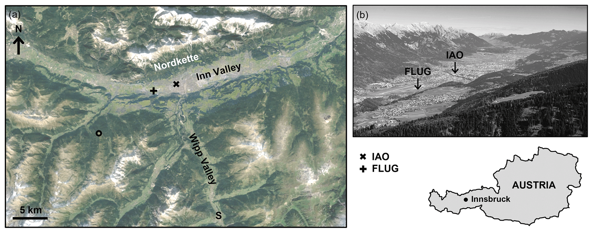
Figure 1(a) Location of the Innsbruck Atmospheric Observatory (IAO) and airport (FLUG) sites in the Inn Valley and Steinach (S) in the Wipp Valley (aerial imagery from © Google Earth). (b) Photograph taken from the position marked with an open circle in panel (a), looking eastwards along the Inn Valley over Innsbruck Airport and the city of Innsbruck. The location of Innsbruck within Austria is shown (bottom right).
Turbulence observations have been made on top of the university building close to the centre of Innsbruck since 2014. In May 2017, the measurement tower was relocated from the northeastern side to the southeastern corner of the university building rooftop as part of the development of the Innsbruck Atmospheric Observatory (IAO). The IAO comprises a suite of instruments for studying urban climate and air quality (Karl et al., 2020). Besides basic meteorological variables and in situ fast-response measurements of wind, temperature, water vapour and carbon dioxide, many trace gases and aerosols are also observed (e.g. Karl et al., 2017; Deventer et al., 2018; Karl et al., 2018), in addition to vertical profiles of wind using a Doppler lidar (Haid et al., 2020, 2021) and temperature and humidity using a microwave radiometer (Rotach et al., 2017). The focus of this study is on the surface–atmosphere exchange of momentum, heat and mass observed using the eddy covariance (EC) technique.
Innsbruck has a small historical core surrounded by predominantly residential areas and industrial zones towards the edges of the city. In the city centre, the buildings are closely packed and typically around six storeys; away from the centre, the buildings are more spread out and slightly lower (three to four storeys). Based on the local climate zones of Stewart and Oke (2012), the majority of the city is open midrise, with compact midrise in the old city core.
The IAO site is located a few hundred metres southwest of the city core. Within a radius of 500 m, the mean building height is 17.3 m, and the mean tree height is 10.1 m. The modal building height, zH, is approximately 19 m. The zero-plane displacement height, zd, is estimated at 13.3 m (based on 0.7 times the modal building height, since the mean building height is reduced by small buildings in courtyards which do not impact the flow; Christen et al., 2009) and the roughness length, z0, at 1.6 m (Grimmond and Oke, 1999). The average land cover composition within 500 m of IAO is 31 % buildings, 24 % paved surfaces, 18 % roads, 19 % vegetation and 8 % water. The Inn river flows from southwest to northeast at a distance of about 100–200 m from IAO (Fig. 2). A more detailed source area analysis is presented in Sect. 3.
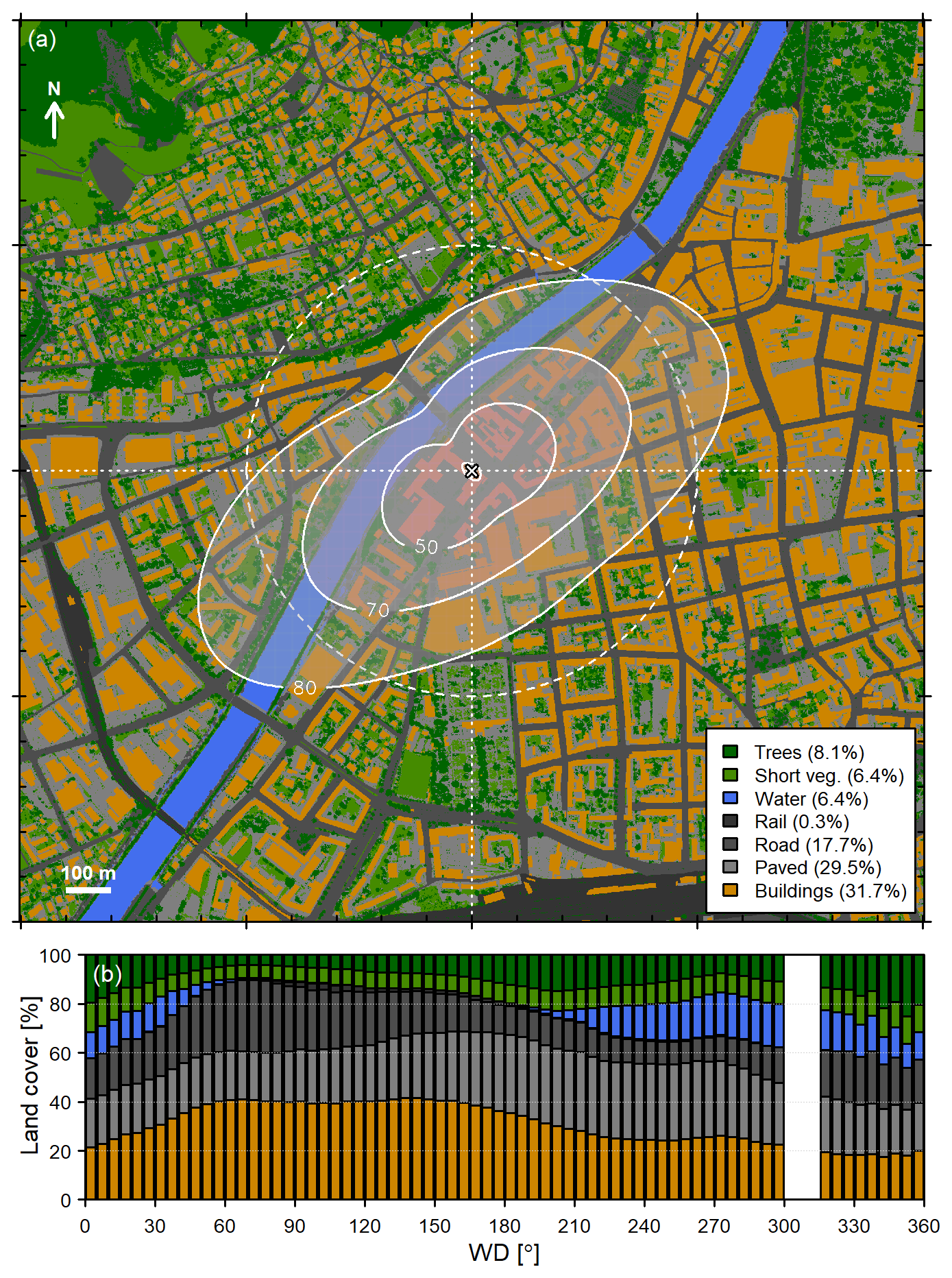
Figure 2(a) Composite source area at IAO for the study period (1 May 2017–30 April 2021) superimposed on land cover (derived from various spatial datasets from Land Tirol, https://data.tirol.gv.at, last access: 17 May 2022). Contours indicate the region comprising 50 %, 70 % and 80 % of the source area, and the circle indicates a distance of 500 m from the flux tower. (b) Average land cover composition by wind direction (no data are available for wind directions of 309 ± 10∘; Sect. 2.3). The aggregated source area composition for the study period is given in the legend.
2.2 Instrument details
A sonic anemometer (CSAT3A, Campbell Scientific) and closed-path infrared gas analyser (EC155, Campbell Scientific) are installed on a lattice mast at a height of 9.5 m above the rooftop of the university building (47∘15′50.5′′ N, 11∘23′08.5′′ E; elevation 574 m a.s.l.), giving a sensor height zs of 42.8 m above ground level (i.e. ). The three wind components, sonic temperature and molar mixing ratios of water vapour and carbon dioxide are logged at 10 Hz (CR3000, Campbell Scientific). A four-component radiometer (CNR4, Kipp & Zonen) at a height of 42.8 m provides incoming and outgoing shortwave and longwave radiation, and temperature and relative humidity are also measured (HC2S3, Campbell Scientific). Rainfall is recorded by a weighing rain gauge (Pluvio, OTT Hydromet) at 2 m above ground level a few hundred metres southwest of IAO (47∘15′35.5′′ N, 11∘23′03.2′′ E).
2.3 Data processing
Data are processed to 30 min statistics using EddyPro (v7.0.7, LI-COR Biosciences). The following standard steps are implemented: despiking of raw data, double rotation to align the wind direction with the mean 30 min flow, time lag compensation by seeking maximum covariance, correction of sonic temperature for humidity (Schotanus et al., 1983) and correction for low- and high-frequency losses (Moncrieff et al., 2004; Fratini et al., 2012). Subsequent quality control removes data when instruments malfunction and during maintenance, when the wind direction (WD) is within ± 10∘ of the direction of sonic mounting (309∘), when the magnitude of the pitch angle exceeds 45∘, when data fall outside physically reasonable thresholds (absolute limits and a despiking test by comparing adjacent data points) or when conditions are non-stationary (following Foken and Wichura, 1996, with a threshold of 100 %). As for other urban studies, no data were excluded on the basis of skewness or kurtosis tests, and the so-called integral turbulence characteristic tests (Foken and Wichura, 1996) have not been applied here. These tests are based on typical values and scaling relations observed over simpler surfaces and thus may not be appropriate for more complex sites (Crawford et al., 2011; Fortuniak et al., 2013; Järvi et al., 2018). Moreover, the applicability of scaling relations to this dataset is one of the aspects we wish to analyse (Ward et al., 2022). Following quality control, 83 %, 72 % and 79 % of sensible heat (QH), latent heat (QE) and CO2 () flux data are available for the 4-year study period from 1 May 2017 to 30 April 2021. All data are presented in Central European Time (CET = UTC+1).
2.4 Additional measurements
Data from short-term field campaigns and various monitoring stations are used here to support analysis of the IAO dataset. As part of the PIANO project investigating foehn winds (Haid et al., 2021; Muschinski et al., 2021; Umek et al., 2021), EC measurements were made at a height of 2.5 m at a grassland site at Innsbruck Airport 3.4 km west of IAO (47∘15′19.4′′ N, 11∘20′34.2′′ E; 579 m a.s.l.; Fig. 1). The station, hereafter referred to as FLUG, was operated from 15 September 2017–22 May 2018 (although data transmission issues resulted in a low data capture rate for September). A similar closed-path eddy covariance system (CSAT3A + EC155) and four-component radiometer (CNR4) to those at IAO were deployed, along with two soil heat flux plates at 0.05 m depth (HFP01, Hukseflux), a temperature and humidity probe (HC2S3), a tipping bucket rain gauge (ARG100, Campbell Scientific) and soil temperature sensors (107, Campbell Scientific). Data were logged at 20 Hz and processed in the same way as for the IAO station (Sect. 2.3). The soil heat flux at the surface was estimated from the average heat flux measured by the plates adjusted to account for the heat stored in the soil layer between the plate and the surface based on the soil temperature at 0.02 m depth. This adjustment makes a considerable difference to the magnitude and phase of the soil heat flux. Comparison of the FLUG dataset with IAO is helpful for distinguishing urban-related characteristics from other controls and offers some insight into spatial variability in the Inn Valley. Additional meteorological data from several stations installed as part of the PIANO campaign (labelled P2–4, P5–8, PAT and THA in Fig. 4) and those operated by the Austrian national weather service ZAMG (Z1–3 in Fig. 4; S in Fig. 1) are also used to investigate spatial variability.
To assist in the interpretation of the IAO dataset, the flux footprint parameterisation of Kljun et al. (2015) was used to provide an indication of the likely source area characteristics and their variability under different conditions. Figure 2 shows the estimated source area for the study period along with the footprint-weighted land cover composition as a function of wind direction. The shape of the source area reflects the predominance of along-valley winds (Sect. 5). Since the area around the flux tower is fairly homogeneous, the land cover composition of the footprint does not change considerably with stability or wind direction. There is a slightly larger contribution from vegetation with increasing stability as the footprint extends further from the tower beyond the city centre. The total impervious (paved and road) surface fraction varies little with wind direction (at about 40 %–50 %), but the proportion of roads is greater for easterly winds (≈ 30 %) than westerly winds (≈ 10 %). The eastern sector also has the greatest proportion of buildings (around 40 %) and the least vegetation (10 %). For the western sector, there is slightly more vegetation (15 %–20 %), and the river comprises up to about 15 % of the source area. The aggregated source area composition for the study period is similar to the average land cover within 500 m (given in Sect. 2.1), with a slightly lower fraction of vegetation and slightly higher fractions of buildings and paved surfaces, reflecting the greater weight of the footprint closer to the tower. On average, 70 %/80 % of the footprint lies within a radius of 500/700 m from the tower.
Meteorological conditions during the study period are summarised in Fig. 3. Innsbruck has a humid continental climate with cool winters, warm summers and strong seasonality. Average monthly temperatures range from −0.1 ∘C in January to 19.8 ∘C in July, and mean annual precipitation is 886 mm (1981–2010 norms for Innsbruck University; ZAMG, 2021). Precipitation occurs throughout the year, with most rainfall in summer (Fig. 3h) when convective storms are frequent. Snow cover down to the valley floor is common during winter and can last several weeks at rural locations along the valley (and longer at higher altitudes); in the city, snow melts much faster due to the higher temperatures, and it is usually quickly cleared from roads. The increased surface albedo, α, during times of snow cover can be seen clearly in Fig. 3a.

Figure 3Time series of daily mean values (shading indicates 10–90th percentiles) of (a) albedo, (b) incoming shortwave radiation, (c) air temperature, (d) specific humidity, q, (e) wind speed, (f) turbulent kinetic energy and (g) sensible heat flux and (h) daily and monthly rainfall for IAO. In panel (h), the thick horizontal bars indicate the 1981–2010 normal monthly rainfall (ZAMG, 2021). The albedo for the FLUG site is also shown in panel (a). In panel (b), the dashed line indicates the top-of-atmosphere irradiance. The top panels show the occurrence of foehn and pre-foehn conditions (see Appendix A for details).
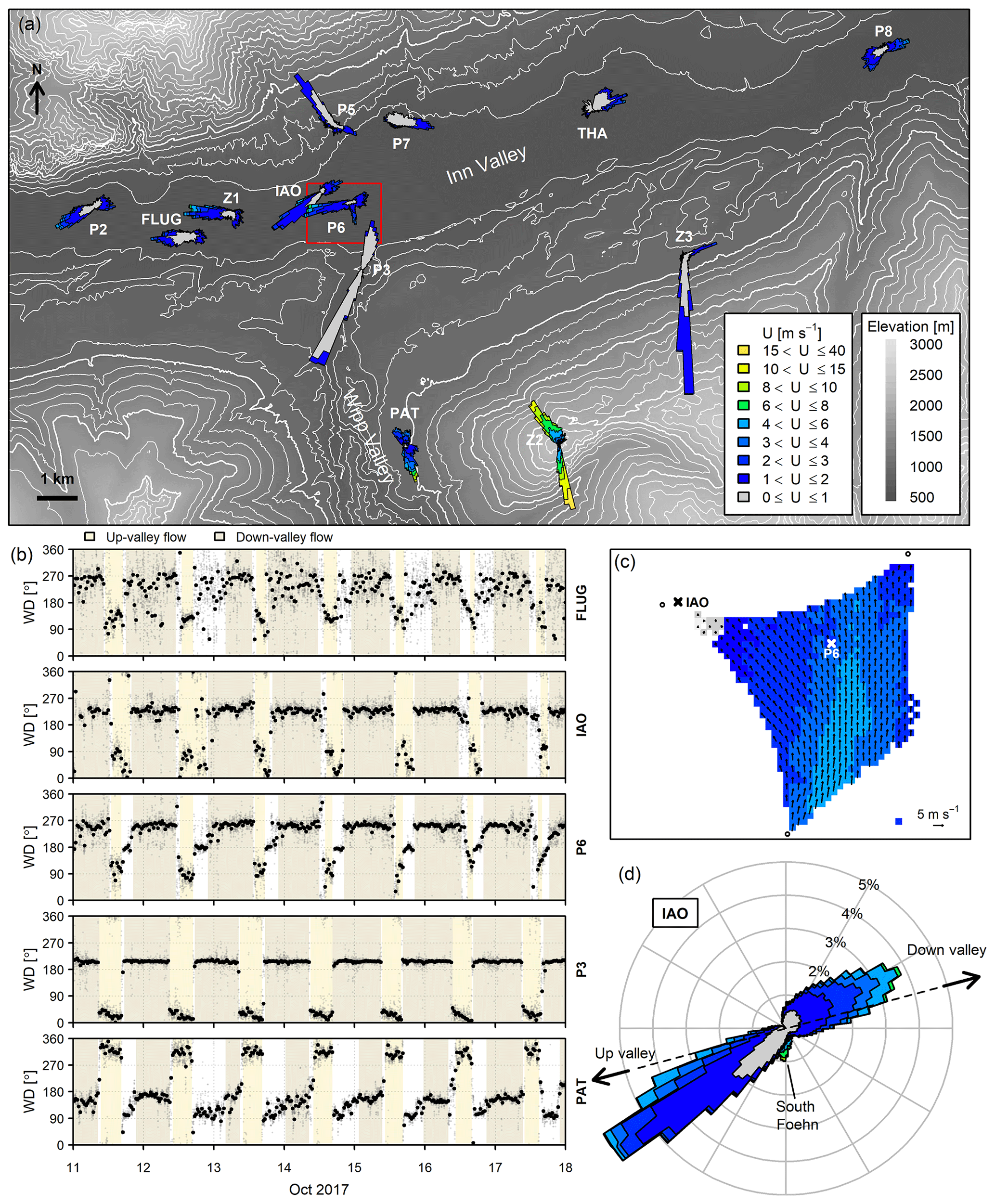
Figure 4(a) Wind roses for stations in and around Innsbruck during Autumn 2017 (all available 30 min data for September–November 2017) overlaid on a digital elevation map (data source: Amt der Tiroler Landesregierung, Abteilung Geoinformation) with thin/thick contours at 100/500 m intervals. (b) Time series of wind direction for selected sites for the mostly clear-sky period of 11–18 October 2017, with the up-valley and down-valley flow shaded. The 30 min data are shown in black and 1 min data in grey. (c) The horizontal wind field (approx. 60 m above ground) at 17:50–18:00 CET on 16 October 2017, as derived from three Doppler wind lidars (circles) performing coplanar scans (see Haid et al., 2020 for details). Colours/arrows indicate wind speed/wind direction; points outside the coplanar field of view are left white. The area shown in panel (c) corresponds to the red box in panel (a) and is about 1.8 km × 1.5 km. (d) Wind rose for IAO during the study period (1 May 2017–30 April 2021). The black line indicates the approximate orientation of the Inn Valley axis at IAO, with the up- and down-valley directions marked. The colour scale for wind speed in panels (c) and (d) is the same as in panel (a).
The study period of 1 May 2017–30 April 2021 was warmer and sunnier than the long-term (1981–2010) average. Overall, 2018 was the warmest year on record in Austria, and 2017, 2018, 2019, 2020 and 2021 were 0.8, 1.9, 1.5 and 1.4 and 0.6 ∘C warmer than normal in Innsbruck (ZAMG, 2021). April 2018 and June 2019 were particularly hot and sunny (4.5 and 4.8 ∘C warmer than normal), whereas September 2017, February 2018 and May 2019 were much cooler (≥ 2 ∘C) than normal (with September 2017 and May 2019 also being much cloudier than normal). While 2017 and 2019 were wetter than normal, 2018 and the first half of 2020 were drier than normal (Fig. 3h). Winter 2017–2018 and 2018–2019 were particularly snowy. At IAO, the observed daily mean temperature ranged from a minimum of −9.2 ∘C in February 2018 to a maximum of 28.1 ∘C in June 2019 (Fig. 3c), and the lowest (highest) temperature recorded was −13.5 ∘C (37.7 ∘C).
5.1 Spatiotemporal variability
Flow patterns in mountainous terrain are extremely complex and show a high degree of spatial variability. Flow is generally channelled along valleys with the dominant wind directions corresponding to the orientation of the valley axis at a particular point (e.g. compare stations in the Inn Valley with stations in the Wipp Valley in Fig. 4a). On mostly clear-sky days with weak synoptic forcing, a valley wind circulation often develops (e.g. Zardi and Whiteman, 2013). These thermally driven mesoscale circulations lead to a twice-daily wind reversal with upslope and up-valley flows during the day and downslope and down-valley flows during the night. Typical thermally driven circulation patterns have been documented previously in the Inn Valley and surrounding valleys (e.g. Vergeiner and Dreiseitl, 1987; Lehner et al., 2019). For flat sites on the valley floor (such as IAO or FLUG), flow tends to be either up or down valley, while for sloping sites up- and downslope winds are also observed (e.g. at sites PAT, P5 and Z3 in Fig. 4a). The upslope winds usually precede the up-valley winds in the morning and the downslope winds precede the down-valley winds in the evening (e.g. easterly downslope winds at PAT in Fig. 4b).
The strength and timing of the valley wind circulation depends on the meteorological conditions and characteristics of the valley such as its width, height, orientation and surface cover (e.g. Wagner et al., 2015; Leukauf et al., 2017). The up-valley flow tends to begin and end earlier in the Wipp Valley than in the Inn Valley around Innsbruck (Dreiseitl et al., 1980). For the October example shown in Fig. 4b, the up-valley flow begins at around 10:00 CET and ends at around 16:30 CET in the Wipp Valley (sites PAT and P3), whereas in the Inn Valley the up-valley flow begins in the afternoon (12:00–15:00 CET) and continues until the evening (18:00–21:00 CET) – although the timing varies considerably throughout the year (see Fig. 5).
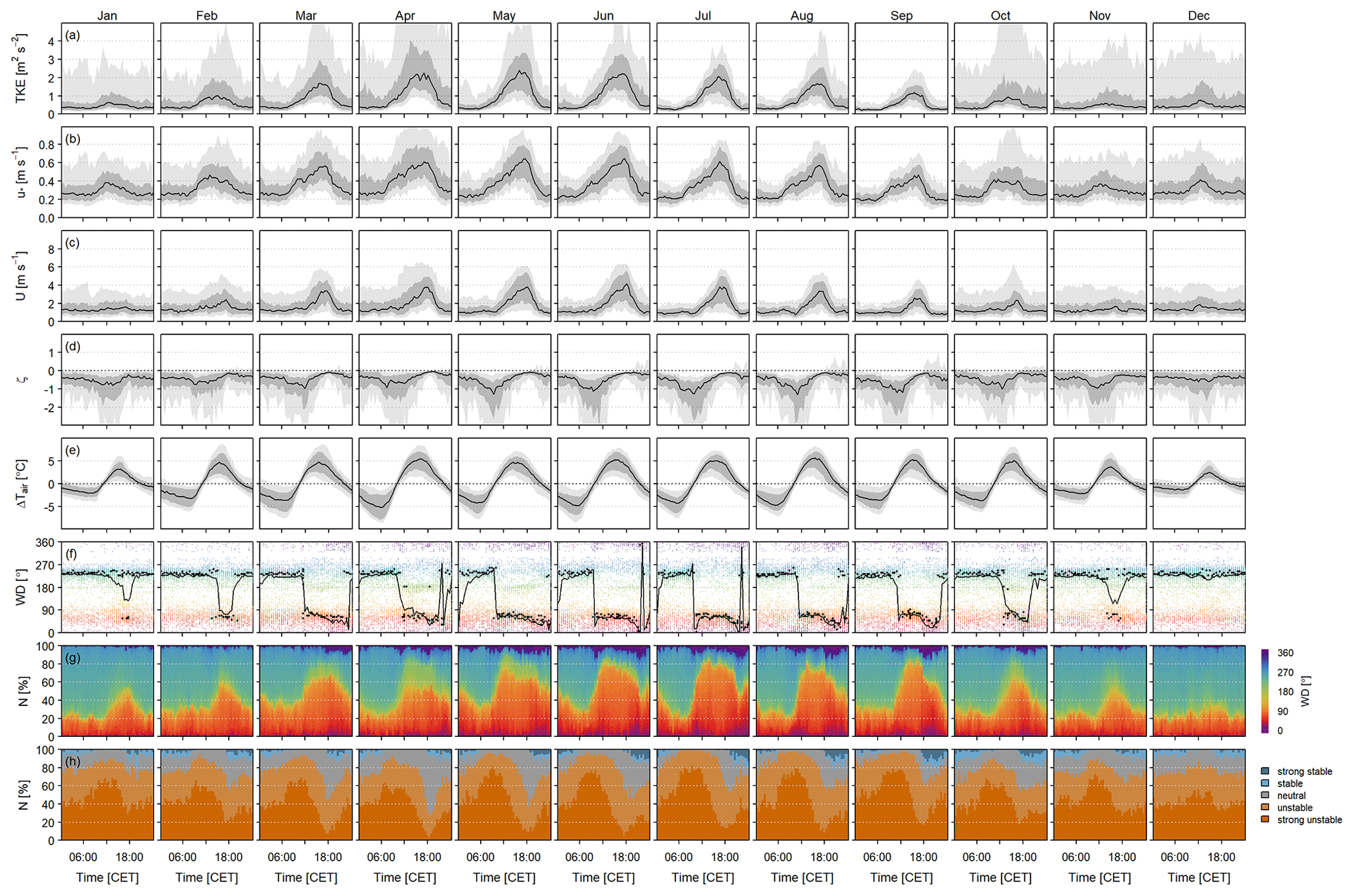
Figure 5Monthly median diurnal cycles (black lines), interquartile ranges (dark shading) and 10–90th percentiles (light shading) of (a) turbulent kinetic energy, (b) friction velocity, (c) wind speed, (d) dynamic stability and (e) the difference between 30 min and daily mean air temperature, ΔTair. (f) Monthly median diurnal cycles (black lines), modal values (black points) and individual 30 min wind directions (coloured points). Normalised frequency distributions of (g) wind direction and (h) stability are separated by month and by time of day. Stability classes are strongly unstable (), unstable (), neutral (), stable (0.1<ζ≤0.5) and strongly stable (ζ>0.5).
At the intersection of two or more valleys, the flow field can be especially complex as the individual valley wind systems with their different magnitudes and forcings interact. Inflow or outflow from side valleys can affect the wind field at some distance from the side valley exit. For example, site P6 in central Innsbruck mainly records the east–west Inn Valley circulation but also detects the southerly katabatic flow from the Wipp Valley, which is seen here as a change in wind direction from easterly (up-valley flow in the Inn Valley) to southerly (down-valley flow in the Wipp Valley) once the flow in the Wipp Valley reverses in the afternoon and before the down-valley flow in the Inn Valley has fully established (Fig. 4a–b). However, this outflow from the Wipp Valley is not seen less than a kilometre away at IAO. Coplanar scans with Doppler wind lidars help to fill in the gaps between point measurements and give an indication of the extreme spatial variability (Fig. 4c; see also Haid et al., 2020). For the example shown, strong southerly wind speeds in the Wipp Valley exit jet can be seen to be mixing with weaker winds in the Inn Valley. Using Doppler lidars over a larger area (e.g. as in Adler et al., 2020, for the Neckar Valley, Stuttgart) would be useful for understanding these interacting flows and their role in the distribution of air pollution within the city.
The long-term wind direction distribution at IAO is roughly bimodal, with more westerly down-valley winds than easterly up-valley winds (Fig. 4d). Although the main wind directions are roughly aligned with the axis of the Inn Valley (about 75–255∘ at IAO), winds blowing down valley are slightly more southerly and winds blowing up valley are slightly more northerly. The reason for this 20–30∘ difference between the valley axis and the main wind directions is not clear. For simplicity, up-valley winds in the Inn Valley will be referred to here as easterly (rather than east–northeasterly) and down-valley winds as westerly (rather than southwesterly).
The strong southerly winds visible in Fig. 4d are foehn events (warm, dry, downslope windstorms). Due to the location of the Brenner Pass (the lowest pass in the main Alpine crest) at the top of the Wipp Valley, strong cross-Alpine pressure gradients can lead to southerly foehn in the Wipp Valley (about 20 % of the time, according to Plavcan et al., 2014), which frequently reaches Innsbruck in spring and autumn (Mayr et al., 2004).
Because mountain winds are restricted by the terrain and closely connected to thermal and dynamical forcing, there are strong temporal signatures in the wind regime and associated turbulence. Figure 5 shows the monthly and diurnal variation in flow, stability and turbulence at IAO for all available data. Although this figure combines various weather types and flow regimes, on average the wind direction at IAO has a clear seasonal and diurnal cycle, with westerly winds overnight and in the morning and easterly winds during the afternoon. The duration of the up-valley flow is greatest during summer, typically beginning late morning (10:00–12:00 CET) and reversing in the late evening (20:00–22:00 CET), while for winter days there is not always a transition to up-valley flow, and if one does occur, the up-valley flow lasts only a few hours during the late afternoon and early evening (Fig. 5f). Similar patterns have been observed previously in Innsbruck (Vergeiner and Dreiseitl, 1987), in the Adige Valley, Italy (Giovannini et al., 2017), in the Rhone Valley, Switzerland (Schmid et al., 2020), and in the western United States (Stewart et al., 2002), for example.
Down-valley wind speeds (U) are 0–2 m s−1 all year round at IAO (but can be larger aloft) and remain fairly constant during the night, although they sometimes show a small maximum in the morning. The up-valley wind speed increases as the up-valley flow establishes and peaks at around 4 m s−1 in the late afternoon, a few hours after the peak in temperature (Fig. 5c, e). Around the time of the wind direction transition, wind speeds are usually very low. These near-zero wind speeds in the middle of the day offer little relief from thermal stress in summer. Friction velocity (u∗) is reasonably high due to the rough urban surface (≥ 0.2 m s−1 even at night; Fig. 5b). Turbulent kinetic energy (TKE) follows a similar temporal pattern to wind speed but with a slightly broader peak and larger values earlier in the day resulting from buoyancy production in the morning (Fig. 5a). Dynamic instability (expressed as the stability parameter ζ= (zs−zd) , where L is the Obukhov length) is greatest during the morning hours; in the afternoon, the atmosphere becomes more neutral as wind speed increases with the strength of the up-valley flow. After the peak up-valley wind, conditions usually become more unstable again, but in a few cases, stable conditions are observed (Fig. 5d, h) when the air temperature is close to surface temperature, wind speeds are low and the sensible heat flux is small and negative.
Stable stratification close to the surface is rarely observed at IAO (ζ>0.1 only 4.7 % of the time). Studies in other densely built urban areas find similarly rare occurrences of near-surface stable conditions (Christen and Vogt, 2004; Kotthaus and Grimmond, 2014a). Even in cities with cold winters, such as Montreal (Bergeron and Strachan, 2010) and Helsinki (Karsisto et al., 2015), the proportion of stable conditions is below about 10 %. Within the study period, no days were identified with persistent near-surface stable stratification at IAO, in contrast to FLUG, which is usually stable overnight (see Sect. 7) and experiences several days with stable stratification in winter, particularly when there is snow cover. Even though strong negative heat fluxes are observed at IAO during foehn in autumn and winter (Fig. 3g, Sect. 5.3), these are mostly classified as neutral due to the high wind speeds. Interestingly, the proportion of unstable conditions in the late afternoon is greater in winter than summer (Fig. 5h), as no strong up-valley wind develops in winter. Heating of buildings also contributes additional energy to the urban atmosphere, which helps to maintain unstable conditions in winter (Sect. 7.1). Note that although the near-surface atmosphere in the city is almost always unstable or neutral, the valley atmosphere is often stably stratified higher up (based on temperature profiles from radiosonde and microwave radiometer; data not shown), and in winter, strong temperature inversions can reduce vertical mixing and contribute to poor air quality. Further research is needed concerning the three-dimensional structure of the mountain boundary layer (Lehner and Rotach, 2018) and particularly the transition between near-surface conditions and the valley atmosphere aloft.
Although several overall trends emerge from the average of this multi-year dataset, when looking at each day individually there is a great deal of variability resulting from the complex urban environment and, more significantly, its orographic setting. Observed wind direction is often highly variable, particularly when the wind speed is low. Some days have easterly flow in the early morning or lasting for several days, which may be low-level cold-air advection from the Alpine foreland. On some days an up-valley wind establishes but is then interrupted and sometimes later resumes and sometimes not. In some cases, this can be related to a drop in solar radiation, rainfall, foehn or outflow from convection. Although easterly winds occur in the afternoon and evening on most days, textbook valley wind days at IAO are surprisingly rare (as has also been reported for the Inn Valley by Vergeiner and Dreiseitl, 1987, and Lehner et al., 2019).
5.2 Valley wind case study
To examine valley wind features more closely, observations at IAO and FLUG from 4 clear-sky days in April 2018 are shown in Fig. 6. A fairly typical valley wind circulation is seen in both the Inn Valley and the Wipp Valley on 18, 19 and 21 April. In both valleys, wind speed is greatest for the well-established up-valley flow, and minima at the times of flow reversal can be seen more clearly than in the averages in Fig. 5c. For these clear-sky conditions, the diurnal course of net radiation and temperature is smooth (radiation data at FLUG in the early mornings is missing because of dew on the sensor). At IAO, surface temperature (Tsfc) is much larger than air temperature (Tair) during the morning, which drives large QH; in the afternoon and evening, Tsfc remains comparable to Tair, and QH is smaller but remains mostly positive. At FLUG, Tsfc is smaller than in the city and slightly larger than Tair during the morning but falls rapidly in the afternoon and drops below Tair well before sunset. Therefore, QH peaks in the morning and becomes negative in the afternoon, supplying energy to maintain large QE until sunset.
At first, many of the characteristics appear similar on 20 April, but the lack of a wind reversal, high wind speeds and the slightly distorted diurnal cycle of potential temperature at Steinach (S in Fig. 1) point to foehn in the Wipp Valley (Fig. 6b, h–i), which seems to reach IAO and FLUG for a very short period in the afternoon. This example highlights the difficulty in distinguishing between different flow regimes in certain cases, and it is quite typical to have days with a valley wind type circulation that are also influenced by foehn or other dynamically forced flows. At IAO and FLUG, the matching of potential temperature to that in the Wipp Valley for a short period and the slightly larger TKE values, coupled with the southerly (rather than easterly) wind at IAO, suggest the foehn reached these stations for a few hours in the afternoon.
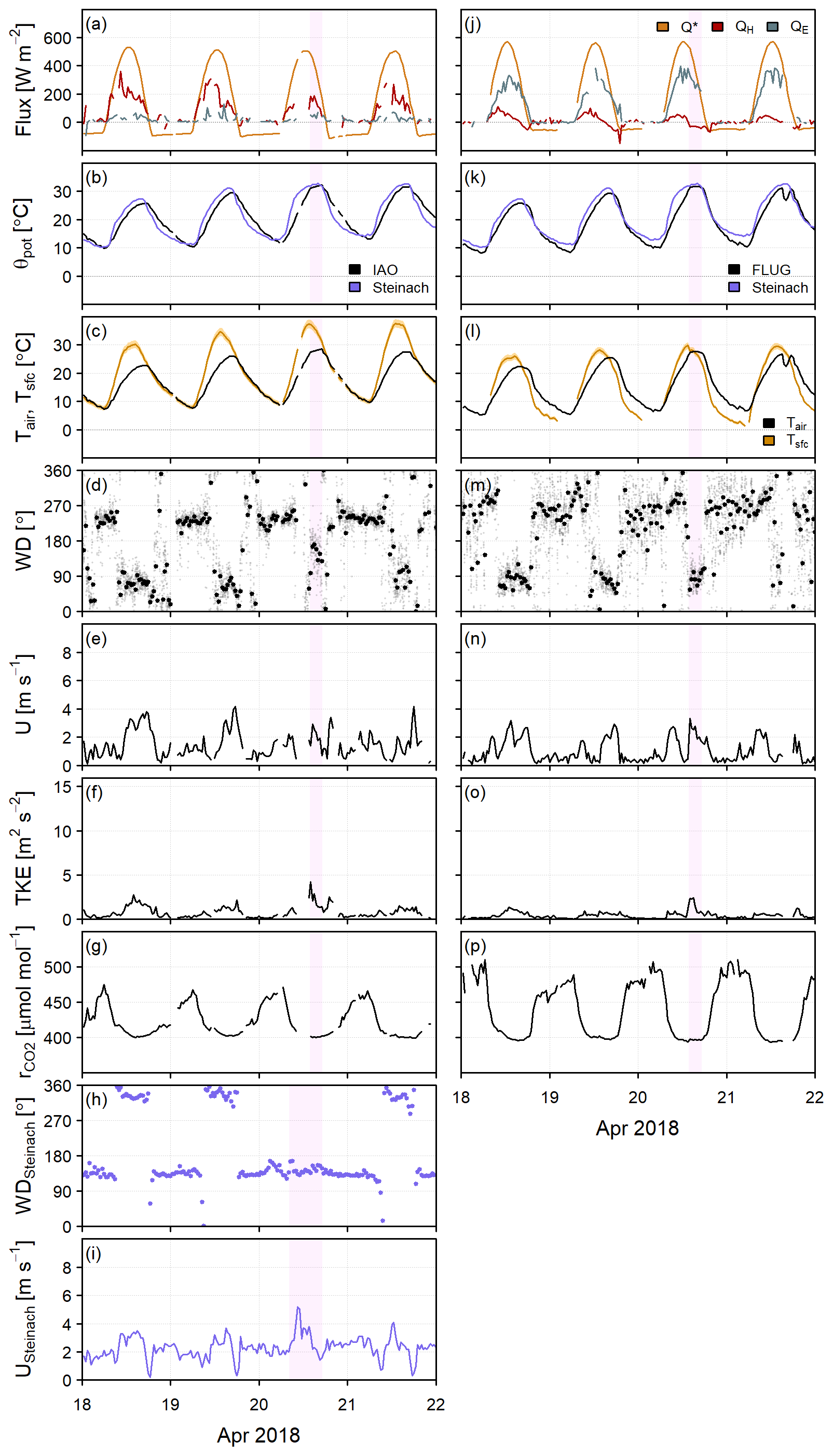
Figure 6Time series of (a, j) net radiation, sensible heat flux and latent heat flux (b, k), potential temperature, θpot, (c, l) air temperature and surface temperature derived from outgoing longwave radiation, assuming an emissivity of 0.95 (shading indicates the uncertainty for emissivities 0.90–1.00), (d, m) wind direction, (e, n) wind speed, (f, o) turbulent kinetic energy and (g, p) CO2 mixing ratio for the clear-sky period of 18–22 April 2018 at (a–g) IAO and (j–p) FLUG. Wind direction (h), wind speed (i) and potential temperature (b, k) at Steinach in the Wipp Valley are also shown. All data are at 30 min resolution; 1 min wind direction is additionally shown at IAO and FLUG (small grey points in panels d and m). Shading indicates times with foehn at each site (see Appendix A for details).
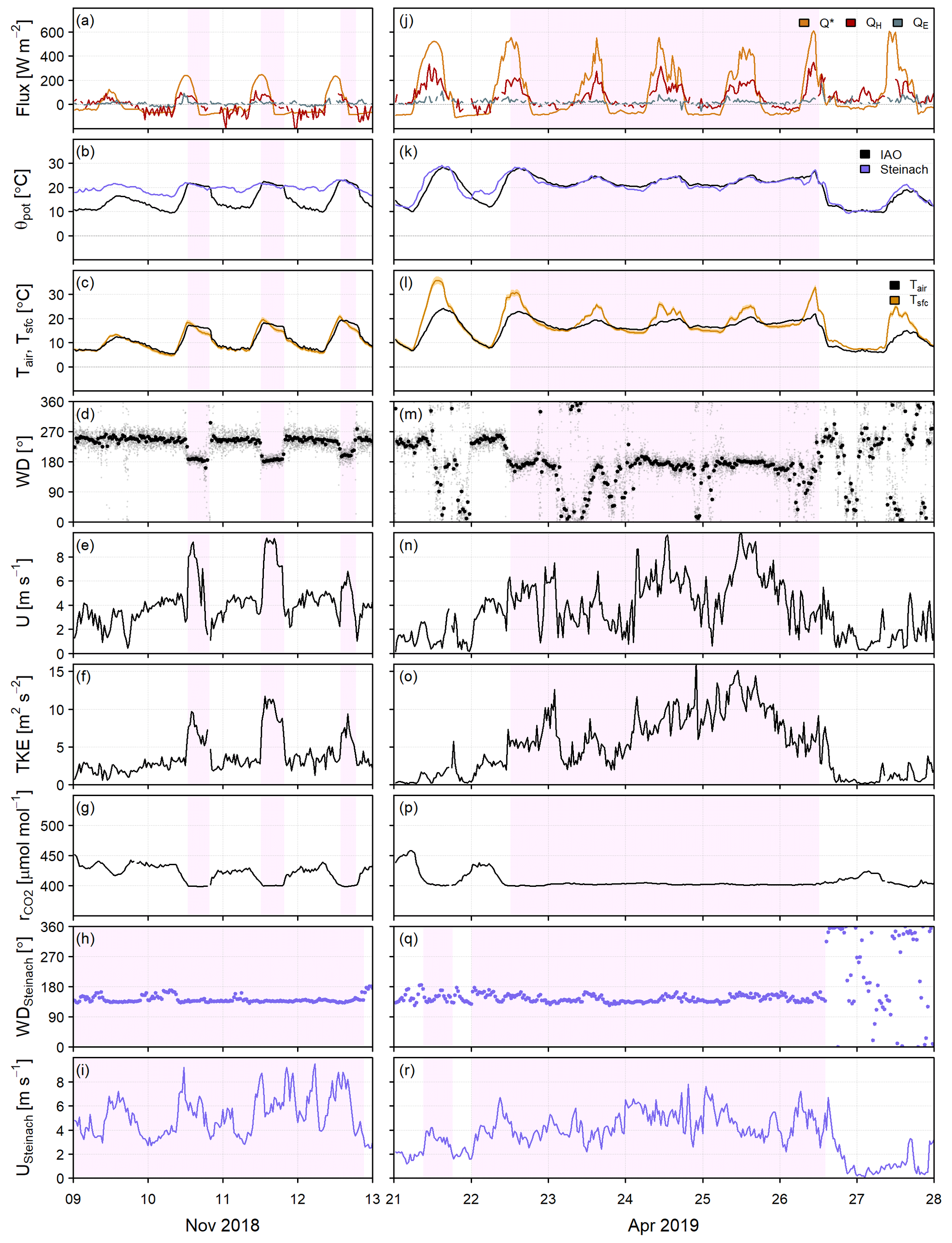
Figure 7As in Fig. 6a–i for the periods (a–i) 9–13 November 2018 and (j–r) 21–28 April 2019. Data are shown for (a–g, j–p) IAO and (h–i, q–r) Steinach.
5.3 Characteristics and effects of foehn
South foehn is most common in Innsbruck in spring (with an average of 22 d during March–May) and autumn (with an average of 13 d during September–November), although there is strong interannual variability (Mayr et al., 2004). The higher frequency of southerly foehn winds in spring and autumn can be seen in the wind direction distributions in Fig. 5f–g. In spring, foehn often reaches the floor of the Inn Valley, sometimes bringing several days of continuous or almost continuous foehn, strong southerly winds and intense mixing in and around Innsbruck, while foehn events tend to be shorter in autumn. Depending on the local strength and depth of the cold pool in the Inn Valley, a breakthrough may occur on one side of the city but not the other (Haid et al., 2020; Muschinski et al., 2021; Umek et al., 2021). Foehn is rare in summer, as the synoptic situation is unfavourable. In winter, the cold pool in the Inn Valley often prevents a breakthrough close to the surface; there may be foehn flow aloft and in the Wipp Valley (Mayr et al., 2004), while closer to the surface strong westerly winds are often observed in and around Innsbruck, so-called pre-foehn westerlies (Seibert, 1985; Zängl, 2003), although these do not necessarily precede a breakthrough. For cases where the cold pool is partially eroded, intermittent foehn can occur in Innsbruck, bringing periods of high wind speeds, intense turbulence and extreme spatial variability in flow and temperature. Thus, depending on the timing and location of the foehn breakthrough, there can be considerable differences in wind speed, wind direction, temperature and humidity within a few kilometres (Muschinski et al., 2021). Foehn in Innsbruck is most common in the afternoons (as the cold pool is often weakest or already dispersed at this time). Processes contributing to the onset and cessation of foehn in Innsbruck are explored in detail in Haid et al. (2020), Haid et al. (2021), Umek et al. (2021) and Umek et al. (2022).
Foehn has a marked impact on conditions in Innsbruck. Particularly during the colder months, foehn can cause the air temperature to increase by 5–15 ∘C and can thus play an important role in snowmelt and sublimation. Many foehn events stand out in time series data as high wind speeds accompanied by substantially enhanced air temperatures (Fig. 3c, e). There is also a clear impact on turbulence; high air temperatures drive large negative QH, even in the city, and TKE values of 5–15 m2 s−2 are not uncommon (Fig. 3f–g). The large spread of TKE values (and wind speed and friction velocity) seen outside the summer months in Fig. 5 is a result of foehn (either a complete breakthrough at the surface or so-called pre-foehn conditions strongly influenced by foehn).

Figure 8As in Fig. 6 for the period 7–14 April 2018 at (a–g) IAO, (j–p) FLUG and (h–i) Steinach.
5.4 Foehn case studies
Figures 7 and 8 present three case studies involving foehn events. For all of these cases, strong southerly winds at Steinach suggest almost continuous foehn in the Wipp Valley, supported by high foehn probabilities from the statistical model of Plavcan et al. (2014). In Innsbruck, there are periods when direct foehn reaches the floor of the Inn Valley, when deflected foehn air reaches IAO and periods when foehn does not reach the surface but nevertheless strongly influences conditions.
For 9 November to the evening of 12 November 2018, there is almost continuous foehn in the Wipp Valley, with some transient breaks or weakening indicated by small changes in wind direction and slight cooling (e.g. overnight 9–10 November 2018). On the afternoons of 10, 11 and 12 November, there is a clear example of a direct foehn breakthrough at IAO, evident from the dramatic increase in temperature, the shift in wind direction from westerly to southerly and the sudden increase in wind speed and TKE (Fig. 7a–g). These events last a few (4–7) hours each, during which the potential temperature at IAO matches the potential temperature in the Wipp Valley (indicating that the atmosphere is well mixed). Overnight, the cold pool in the Inn Valley re-establishes, and pre-foehn westerly winds return near the surface, while foehn is still present aloft and in the Wipp Valley. On 9 November, foehn does not reach IAO, possibly due to a more persistent cold pool resulting from the lower radiative input on this day. However, the impact of foehn is still felt in Innsbruck with strong pre-foehn westerlies and large TKE.
The situation is somewhat different for the April 2019 case study (Fig. 7j–r). Foehn is continuously observed at IAO from around midday on 22 April to midday on 26 April. The air temperature remains high throughout this period (it is around 10 ∘C warmer overnight than without foehn on 21 and 27 April), and in contrast to Fig. 7b, the potential temperature closely follows that in the Wipp Valley for the whole period. The wind speed is mostly high, and the wind direction is mainly southerly, but northeasterly winds are observed at times, indicating that southerly winds are not a necessary condition for foehn at IAO. Weak northerly or easterly winds are often a result of foehn air being deflected from Nordkette before reaching IAO (Haid et al., 2020; Umek et al., 2021). Intense turbulent mixing is evident from the high TKE values. Typically, CO2 accumulates close to the surface overnight, leading to a peak in the CO2 mixing ratio () in the early morning hours before turbulent mixing increases and the boundary layer begins to grow (Reid and Steyn, 1997; Schmutz et al., 2016). During foehn, however, the sustained mixing prevents the usual buildup of CO2 (and other pollutants) in the nocturnal boundary layer, so that there is very little diurnal variation, and the usual early morning peak (visible on days without foehn overnight in Innsbruck) is not seen (compare Fig. 7g, p). Because of the increased mixing and influx of clean air during foehn, the nocturnal CO2 mixing ratios are generally lower during days with at least some foehn than on clear-sky days with calm nights (e.g. compare with Fig. 6).
For the third case study (Fig. 8), data are presented for both IAO and FLUG to illustrate differences due to location and surface cover. On 7, 8, 9, 10 and 13 April 2018, foehn reaches the Inn Valley during the daytime and is interrupted during the night; on 11–12 April, there is no apparent interruption of the foehn (note, again, the flattened diurnal cycle of ). While the wind direction at IAO during the foehn periods on 7, 8 and 13 April is consistently southerly, some easterly or northerly winds are observed on 9–12 April. At FLUG, southerly foehn often appears as easterly winds since direct southerly flow is blocked in many cases by the mountains to the south of the site. During the interruptions to foehn in the Inn Valley, the potential temperature at IAO and FLUG drops below that in the Wipp Valley, and pre-foehn westerlies are seen at both sites.
The increase in air temperature associated with the arrival of warm foehn air affects the near-surface temperature gradient and thus the heat fluxes. Studies investigating the impact of downslope winds on snowmelt over prairies in Alberta, Canada (MacDonald et al., 2018), and farmland in Hokkaido, Japan (Hayashi et al., 2005), reported reduced or negative QH and enhanced QE during foehn-type winds. A similar effect is seen at FLUG. During foehn, the elevated air temperature can exceed the surface temperature and cause QH to decrease and turn negative long before sunset (Fig. 8j, l). Enhanced QE is sometimes seen accompanying the reduced QH (e.g. 7 and 8 April; Fig. 8j). QH at IAO is usually positive but during foehn or pre-foehn tends to be smaller and can even be negative. Higher surface temperatures in the city mean that, even during foehn, Tair rarely exceeds Tsfc by much, so this effect is somewhat reduced. However, during the colder months, this smaller temperature gradient acts to reduce QH and can even result in negative QH values, which are unusual for a city centre site. Since evaporation is limited by the availability of water (not energy), enhanced QE is not observed during foehn at this urban site. However, at a suburban site in Christchurch, New Zealand, with greater moisture availability due to 56 % vegetation cover, negative QH and enhanced QE were observed during foehn (Spronken-Smith, 2002).
6.1 Orographic shading
Similar to the way that buildings reduce the sky view factor in urban canyons (e.g. Johnson and Watson, 1984), the surrounding terrain reduces the sky view factor in valleys (Whiteman et al., 1989). This orographic shading effect is generally largest in deep, narrow valleys with a north–south orientation (e.g. Matzinger et al., 2003), but even in wider valleys, local sunrise can be later and local sunset earlier compared to sunrise and sunset over flat terrain. At IAO, sunrise occurs on average 45 min later and sunset 50 min earlier, although this varies throughout the year. The longest delay to sunrise is 90 min in winter, whereas the longest shift in sunset is 80 min in summer (Fig. 9a–b). Since the orographic shading effect depends on the shape of the terrain relative to solar angle, for IAO the effect is smallest not in mid-summer when the sun is highest in the sky but when the solar azimuth angles around sunrise and sunset are aligned with the Inn Valley in spring and autumn. Although straightforward to calculate from a digital elevation map and solar angles (here determined using the R package solaR; Perpiñán, 2012), orographic shading is highly spatially variable, and for different locations within the city, there can be differences in local sunrise/sunset times of some tens of minutes. Towards the edges of the city at the base of the north-facing slope, the total solar radiation receipt is reduced substantially.
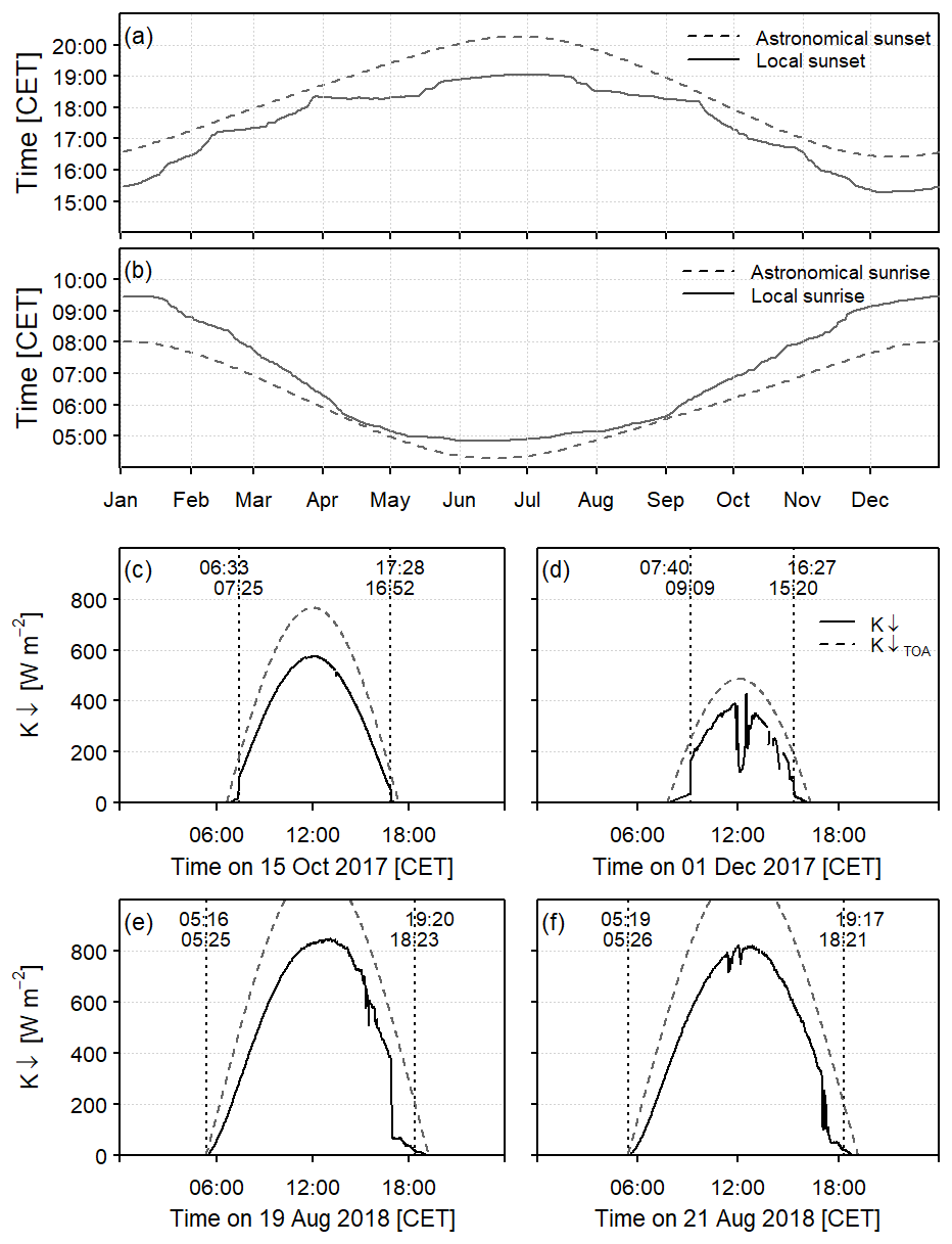
Figure 9Time of local and astronomical (a) sunset and (b) sunrise at IAO. Observed incoming shortwave radiation (1 min data) for example days, illustrating the effect of (c, d) orographic shading and (e, f) orographic shading plus afternoon cloud cover around the surrounding peaks. In panels (c)–(f), local sunrise and sunset are marked by dotted vertical lines, and the times of local and astronomical sunrise and sunset are shown. The incoming shortwave radiation at the top of the atmosphere K↓ TOA is also shown (see text for details).
The overall impact of orographic shading on the annual solar radiation receipt at IAO is small, with around 2 % less solar radiation received over the course of the year (this is an upper limit assuming clear-sky conditions and that incoming shortwave radiation, K↓, is zero before/after local sunrise/sunset; in reality, there is a small diffuse component). The impact is larger in winter when incoming daily solar radiation is reduced by about 10 %. Although the long-term impact of orographic shading is small at IAO, the sudden change in K↓ at local sunrise or sunset can be substantial (∼ 100 W m−2 within a few minutes; Fig. 9c–d). A secondary shading effect is also observed. On mostly clear-sky days, cumulus clouds often form above the mountain peaks during the afternoons, causing an even earlier drop in solar radiation since the Sun is blocked by clouds before it is blocked by terrain (Fig. 9e–f). For a sloped grassland site in the Swiss Alps, a large and rapid drop in K↓ at local sunset has been shown to result in a drop in surface temperature of 10 ∘C in less than 10 min (Nadeau et al., 2013). Such an effect would likely be smaller in urban areas due to the large thermal capacity of building materials and the additional anthropogenic heat supply (which does not stop abruptly at sunset). Note that, for sloping sites, K↓ may far exceed that over flat terrain (depending on the slope and aspect of the surface relative to the direct beam solar radiation), the shape of the diurnal cycle can be very asymmetrical and its peak may be shifted earlier or later (Matzinger et al., 2003; Nadeau et al., 2013).
The surrounding terrain also affects longwave exchange. The smaller the sky view factor and greater the proportion of the radiometer field of view taken up by relatively warm valley slopes, as opposed to cold sky, the larger the observed incoming longwave radiation L↓ (Whiteman et al., 1989). It was not possible to quantify this effect here; however, it is expected that L↓ is larger in Innsbruck than over an equivalent site in flat terrain. The principle is analogous to enhanced L↓ in street canyons due to emissions from surrounding buildings (Oke, 1981).
6.2 Atmospheric transmissivity
Atmospheric transmissivity was investigated using a clearness index which expresses the ratio of observed K↓ to incoming shortwave radiation at the top of the atmosphere K↓ TOA (calculated assuming a solar constant of 1367 W m−2; Peixoto and Oort, 1992). The mean value of the clearness index for the study period is 0.45 (K↓>5 W m−2). Considering clear-sky days only (see Appendix A), the midday (11:00–15:00 CET) clearness index is 0.74 and shows some seasonal variability (Fig. 10a), with the highest value in early spring at 0.78 when the boundary layer height is considerable and water vapour content is low, and lower from summer through to winter at 0.68–0.73. This is attributed to increased moisture and aerosols in the atmosphere in summer and reduced boundary layer growth and increased pollutant concentrations in winter. Although air quality is a major issue for Alpine valleys, it is even more critical for larger cities in complex terrain, such as Mexico City (Velasco et al., 2007), where air pollution was found to deplete K↓ by 22 % compared to a rural reference site (Jáuregui and Luyando, 1999).
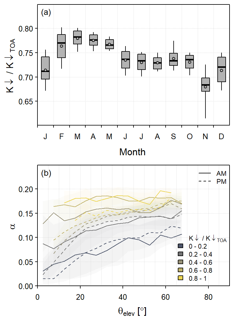
Figure 10(a) Monthly box plots of the midday (11:00–15:00 CET) clearness index at IAO for clear-sky days. Boxes indicate the interquartile range, whiskers the 10–90th percentiles and the median and mean are shown by horizontal bars and points, respectively. (b) Albedo (K↓>5 W m−2; times with snow cover have been removed) at IAO versus elevation angle separated by clearness index and into morning (AM) and afternoon (PM) periods. Lines indicate binned median values and shading the interquartile range.
6.3 Albedo
At IAO, the average midday (11:00–15:00 CET) albedo is 0.16. This is within the range of values previously obtained for European cities, such as 0.08 in Łódź (Offerle et al., 2006), 0.11 in Basel (Christen and Vogt, 2004), 0.11 and 0.14 for two sites in London (Kotthaus and Grimmond, 2014b) and 0.16–0.18 in Marseille (Grimmond et al., 2004). For one of the London sites and the Marseille site, light-coloured roof surfaces below the radiometers led to observed albedos that were probably higher than the bulk local-scale albedo. Similarly, at IAO, the radiometer source area is mainly comprised of light-coloured roof and concrete surfaces, and thus, the measured outgoing shortwave radiation (K↑) is probably slightly higher than the local-scale average.
As there is negligible vegetation within the radiometer field of view, α is fairly constant all year round, except when snow covers the surface (Fig. 3a). In the city, snow is usually cleared from roads within a few hours and melts quickly on roofs. Thus, in contrast to the rural surroundings, α at IAO usually decreases quickly and returns to the lower non-snow-covered values after a few days (although heavy snow cover in January 2019 remained on rooftops and uncleared areas for longer). Snow cover at IAO and FLUG was determined from a visual inspection of webcam images from the university and Innsbruck Airport. When there is a thick covering of fresh snow, α increases to about 0.4 at IAO and 0.7 at FLUG. This difference between urban and rural values is partly due to the large proportion of non-snow-covered vertical walls seen by the IAO radiometer and partly due to the short duration of pristine snow cover in the city (before clearing or melting occurs). The IAO values obtained here are also lower than for a suburban site in Montreal (0.6–0.8), where the duration of snow cover is much longer (Järvi et al., 2014). During non-snow periods, α at FLUG is about 0.21 (September–May dataset), similar to that observed at the Neustift FLUXNET site – a grassland site in the nearby Stubai Valley (Hammerle et al., 2008).
Although there is little seasonal trend in α at IAO, there is considerable variability associated with solar elevation angle (θelev), azimuth angle, cloud cover and rainfall. Due to the location of the IAO radiometer at the southeastern edge of the building, shading of the street below during the afternoon causes asymmetry in the diurnal cycle of α. For similar K↓ and θelev, α is up to about 0.05 smaller in the afternoon than the morning. This difference is greatest during sunny conditions and almost disappears for high elevation angles (Fig. 10b). α is much larger under clear-sky conditions (0.15–0.20) compared to cloudy conditions (close to 0.10). Shortly following rainfall, the albedo drops by about 0.03 and steadily rises over the following 6 h as the surface dries (Fig. 11a).
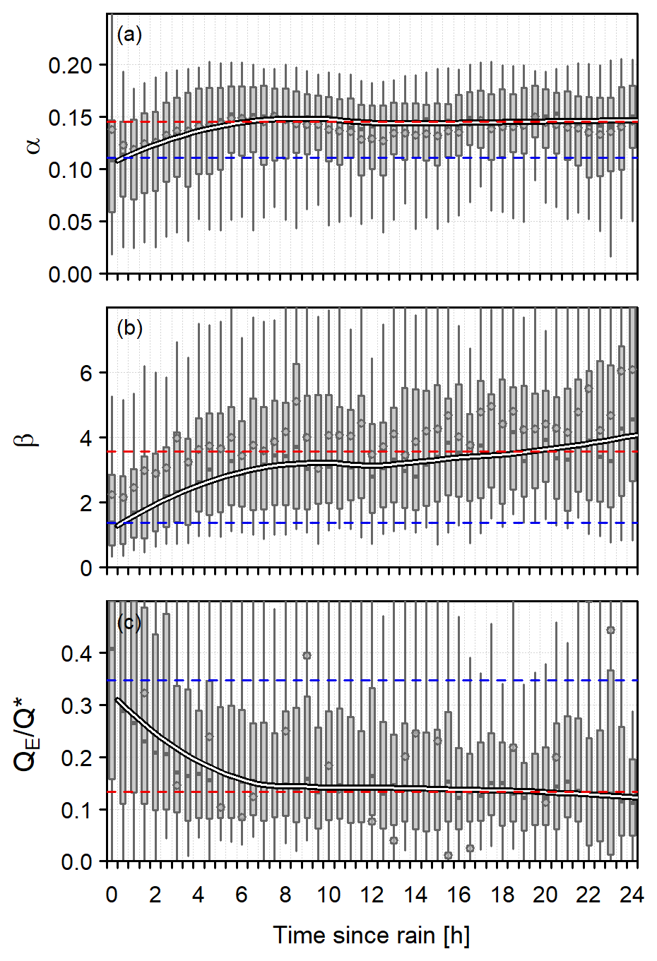
Figure 11Box plots of (a) albedo, (b) Bowen ratio and (c) the ratio of the latent heat flux to net radiation binned by time since measured (>0 mm) rainfall for daytime (K↓>5 W m−2) data only at IAO. The thick line is a loess curve through the median values; the red dashed line indicates the mean of these values between 12 and 24 h since rain (i.e. reasonably dry conditions) and the blue dashed line for the first two boxes (i.e. wet conditions less than 1 h since rainfall).
6.4 Radiative fluxes
Figure 12 shows the seasonal and diurnal patterns and interannual variations in radiation and energy fluxes at IAO for the 4-year study period. For comparison, data for FLUG are also shown for the period that the site was operational. Although interannual variability in the radiation and energy fluxes is generally small (Fig. 12l–u), some differences can be identified. The shortwave radiation components show the most variability, and the particularly cloudy months of September 2017 and May 2019 can be clearly seen in Fig. 12l. The effect of this reduced K↓ is also visible in K↑, the net radiation (Q*) and the sensible heat flux (Fig. 12m, p, r) and, to a lesser extent, in the outgoing longwave radiation (L↑; Fig. 12o). Except for cloudy September 2017 and February 2018, the fluxes at IAO for the period that FLUG was operational are very similar to those over the whole dataset.
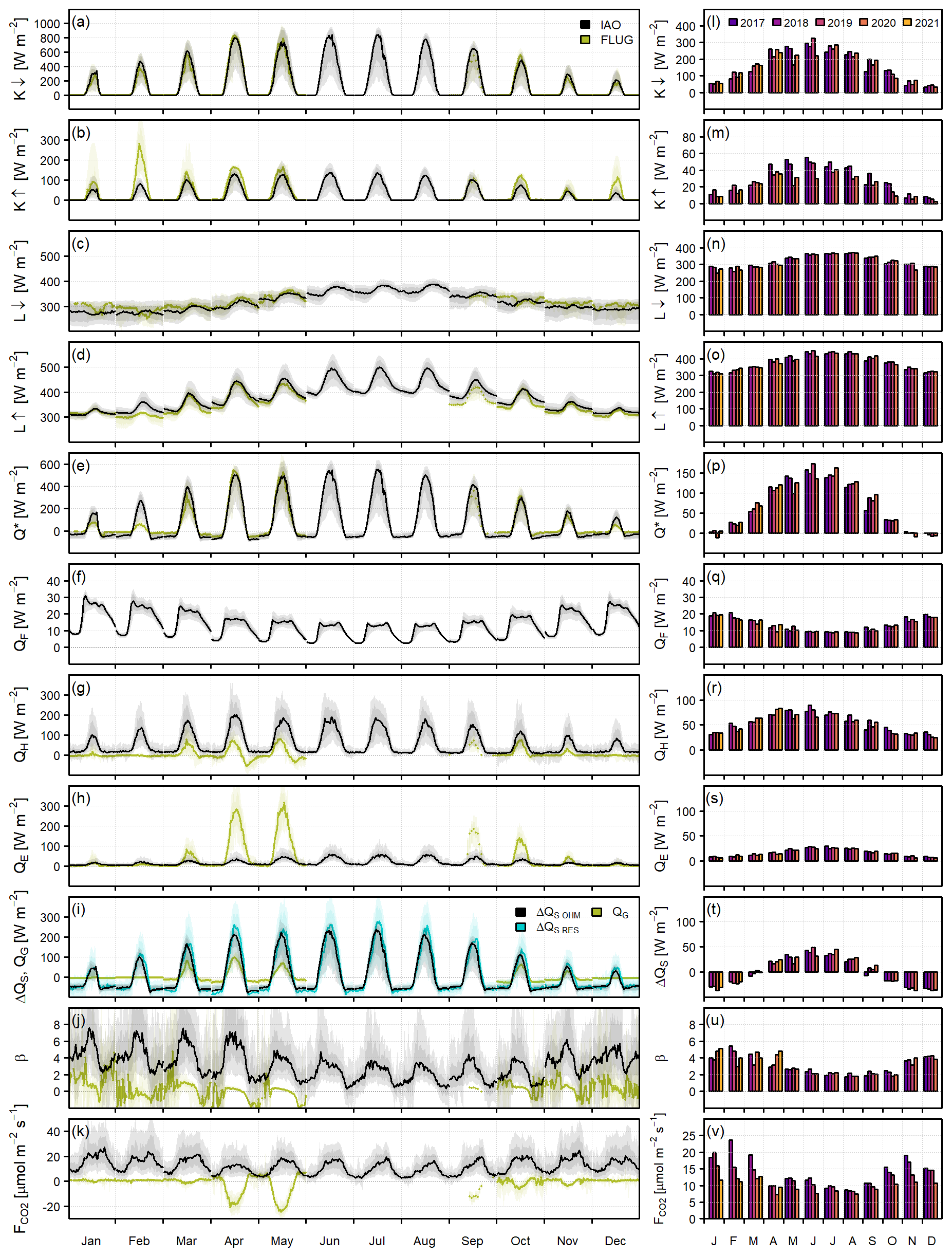
Figure 12(a–k) Monthly median diurnal cycles (lines), interquartile ranges (dark shading) and 10–90th percentiles (light shading) of radiative fluxes, energy balance terms and carbon dioxide fluxes. (a) Incoming shortwave radiation. (b) Outgoing shortwave radiation. (c) Incoming longwave radiation. (d) Outgoing longwave radiation. (e) Net all-wave radiation. (f) Anthropogenic heat flux. (g) Sensible heat flux. (h) Latent heat flux. (i) Storage heat flux. (j) Bowen ratio. (k) Carbon dioxide flux. All available data for IAO and FLUG are shown in black and green, respectively. In panel (i), the net storage heat flux (ΔQS), estimated using the Objective Hysteresis Model (OHM) and estimated as the energy balance residual (RES), is shown for IAO, and the ground heat flux (QG) is shown for FLUG. (l–v) Bar plots of daily mean fluxes at IAO are separated by month and by year (colours). In panel (t), the storage heat flux is estimated using OHM. Note the different y-axis limits.
Of the four radiation components, K↓ has the largest annual cycle, providing an average of 38 W m−2 (3.3 MJ m−2 d−1) in December and 289 W m−2 (25.0 MJ m−2 d−1) in June at IAO. This is the main energy input to the surface. As the albedo is fairly small and constant throughout the year, the net shortwave radiation () and the net all-wave radiation Q* during daytime closely follow K↓. Comparing radiative fluxes for the same time period, K↓ at IAO and FLUG is very similar (for 30 min values, the square of the correlation coefficient r2=0.97), which is as expected given the close geographical proximity of the sites, but the extended period of snow cover at FLUG leads to much higher K↑ than at IAO during winter (Fig. 12b). This also leads to a substantial difference in Q* (Fig. 12e). Average Q* for February 2018 was 27 W m−2 (2.3 MJ m−2 d−1) at IAO compared to only 2 W m−2 (0.2 MJ m−2 d−1) at FLUG.
Outgoing longwave radiation follows a clear diurnal cycle all year round, which is of considerable amplitude (>100 W m−2) during summer. Only on days with very little solar radiation does L↑ depart from this pattern. L↑ is higher in summer than in winter because the surface temperature is higher. Compared to the grassland site, L↑ is larger in the city and remains higher in the evenings and overnight (Fig. 12d), as stored heat is slowly released from the urban fabric and anthropogenic activities continue to provide energy. Incoming longwave radiation has a less repeatable diurnal pattern, as it is influenced to a much greater extent by cloud cover and thus is more variable, particularly during winter. Only on clear-sky days does L↓ follow a smooth diurnal cycle. While the net shortwave radiation () is positive all year round (zero at night), the net longwave radiation () is negative all day and all year as L↑ almost always exceeds L↓ (except for a few cases (<2 %), which occur mainly when the surface is covered with snow).
From November to January, the net longwave loss is similar to the net shortwave gain, and daily Q* is close to zero (Fig. 12p). The magnitudes of the net longwave loss and the net shortwave gain both increase towards summer, but the net shortwave gain increases faster, resulting in a substantial net radiative energy input. Average Q* is −4 W m−2 (−0.4 MJ m−2 d−1) in December and 159 W m−2 (13.7 MJ m−2 d−1) in June with typical peak daytime values of 120 W m−2 in December and 540 W m−2 in June/July. At night, Q* is negative as a result of longwave cooling, more so in summer than winter, and more so at the urban site than the rural site (Fig. 12e).
7.1 Anthropogenic heat flux
In the urban environment, the available energy is supplemented by additional heat released from human activities (Oke et al., 2017). This anthropogenic heat flux (QF) includes energy use in buildings (QB) and for transportation (QV), as well as energy from human metabolism (QM). Here QF was estimated as described in Appendix B using a typical inventory approach similar to that at other sites (e.g. Sailor and Lu, 2004). For this area of Innsbruck, QF is estimated to provide an average of 9–19 W m−2 d−1 (of which approximately 1, 5 and 3–14 W m−2 are from QM, QV and QB, respectively). QF is highest in the coldest months when the demand for building heating is greatest and most of the interannual variability (Fig. 12q) is due to temperature. However, QF is lower than would otherwise be expected in March–April 2020 and November 2020–January 2021 due to a substantial reduction in traffic during COVID-19 lockdowns (no information was available about how building energy use changed over this period, however). The magnitude of QF for this site in the centre of a small city lies between the typical values of 5–10 W m−2 found for suburban sites (e.g. Pigeon et al., 2007; Bergeron and Strachan, 2010; Ward et al., 2013) and the much higher values (>40 W m−2) obtained for central sites in larger and more densely built cities (e.g. Ichinose et al., 1999; Nemitz et al., 2002; Hamilton et al., 2009). QF is about 20 % less on non-working days (i.e. weekends and holidays) compared to working days.
Although the anthropogenic energy input is small compared to the net radiation in summer, QF becomes a more significant source of energy in winter. During winter daytime, QF accounts for around 20 % of the available energy (i.e. ). On a 24 h basis, QF increases the available energy from close to zero to around 20 W m−2 in winter (Fig. 12p, q), which helps to maintain a positive sensible heat flux all year round (Fig. 12g, r). Furthermore, QF affects the difference in available energy between the city and rural surroundings (where QF is assumed to be zero), enhancing the spatial variability in turbulent fluxes which could impact local circulation patterns and cold pool evolution.
7.2 Net storage heat flux
The net storage heat flux, ΔQS, is another important term in the urban energy balance but very difficult to measure directly (Offerle et al., 2005a). Here, two commonly used approaches are used to estimate ΔQS. The first approach is the Objective Hysteresis Model (OHM) of Grimmond et al. (1991), which calculates ΔQS from Q*, the rate of change of Q* and empirical coefficients for different land cover types (see Appendix C for details). The second approach estimates ΔQS as the residual (RES) of the energy balance (). Both approaches have limitations. OHM relies on coefficients derived from a handful of observations or simulation studies and does not account for changes in surface conditions (e.g. soil moisture), while the residual approach ignores advection, assumes the energy balance is closed (which it likely is not) and errors in the other energy balance terms collect in the estimate of ΔQS. Nevertheless, for IAO, the two storage heat flux estimates are in remarkably good agreement (Fig. 12i). The magnitude of ΔQS_OHM is slightly smaller than ΔQS_RES, but the seasonal and diurnal cycles are well represented overall. This contrasts with two UK sites where OHM was found to perform poorly in winter, underestimating the daytime storage release in central London and overestimating the storage release over the whole day in suburban Swindon (Ward et al., 2016).
During the day, when heat is being stored in the large thermal mass of the buildings and roads, ΔQS is large and positive (with peak daytime values of 230 W m−2 in summer and 40 W m−2 in winter). At night, stored heat is released to the atmosphere. The substantial negative ΔQS ( W m−2) during nighttime supports the positive sensible heat fluxes and appreciable longwave cooling. The larger the available thermal mass (i.e. the more densely built the city), the greater the potential to store heat (hence, the ground heat flux at FLUG is much smaller in comparison). From April to August, more heat is stored in the urban fabric than released, whereas the opposite is true from October to February (Fig. 12t). In theory, the losses and gains should cancel over the year, but here ΔQS_OHM and ΔQS_RES yield a small net gain (2.4 and 6.5 W m−2), similar to previous studies (Grimmond et al., 1991).
7.3 Turbulent heat fluxes
As has been observed at other densely built city centre sites, such as Basel (Christen and Vogt, 2004), Łódź (Offerle et al., 2005a) and London (Kotthaus and Grimmond, 2014a), the sensible heat flux generally remains positive all day and all year round at IAO (Fig. 12g, r). Daily average QH ranges from 28 W m−2 (2.4 MJ m−2 d−1) in December to 77 W m−2 (6.7 MJ m−2 d−1) in June. Peak average daytime QH is highest in April and remains fairly constant above 180 W m−2 in April–August. Average nighttime values are positive at around 10–15 W m−2. The latent heat flux is much smaller (Fig. 12h, s), with daily average values from 7 W m−2 (0.6 MJ m−2 d−1) in December–January to 26 W m−2 (2.3 MJ m−2 d−1) in June–July. Peak daytime values average around 55 W m−2 in summer (i.e. less than a third of peak QH values), and QE remains small and positive overnight (4–8 W m−2). Thus, most of the available energy is directed into either heating the atmosphere (QH) or heating the surface (ΔQS).
7.4 Energy partitioning
To facilitate comparison between sites, energy fluxes are often considered relative to the net radiation. The values of the resulting ratios depend on the time of day considered (e.g. midday, daytime, and 24 h) and the season (Fig. 13). At IAO, the month-to-month variation in the energy flux ratios is quite small from late spring to early autumn, but the ratios change more quickly (and are more variable) in winter when the energy supplied is smaller and days are shorter. is 0.42, is 0.40 and is 0.14 on average during summer daytime. During winter, is larger (around 0.65) and is smaller, partly due to the additional anthropogenic energy input from building heating and the tendency for heat that has been stored in the urban environment to be released. Daytime is lowest in February–April at <0.1 and highest in August–October at 0.14–0.15, roughly corresponding to seasonal variability in rainfall (Fig. 3h); the small amount of vegetation likely makes only a minor contribution to increased evapotranspiration during summer. The Bowen ratio () is largest between January and April at 5.4–5.5 and decreases in the summer months to a minimum of 2.5 in August (average daytime values).
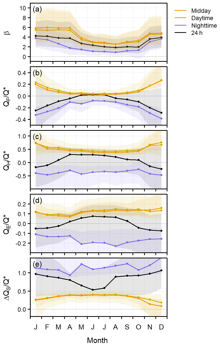
Figure 13Energy partitioning at IAO for different subsets, with midday (11:00–15:00 CET), daytime (K↓>5 W m−2), nighttime ( W m−2) and 24 h. Lines indicate the monthly median values and shading the interquartile range for (a) the Bowen ratio and for (b) the anthropogenic heat flux, (c) sensible heat flux, (d) latent heat flux and (e) net storage heat flux (calculated using OHM) normalised by net radiation.
As there are few vegetated or pervious surfaces in the centre of Innsbruck, there is little possibility for rainwater to infiltrate and be stored in the urban surface, so the effect of rainfall on the surface energy balance is short lived. When surfaces are wet shortly after rainfall, enhanced evaporation rates are observed (Fig. 11b–c). Directly following rainfall, is around 0.35 and β around 1.4; over the next 6–12 h, falls to around 0.13 and β increases above 3.5. These values represent averages over the whole dataset; naturally, there is variation in magnitude and drying time according to season, weather conditions and the amount of precipitation. However, the impact of rainfall seems to be quite short in Innsbruck. At (sub-)urban sites with a greater proportion of pervious surfaces, the process can take several days (Ward et al., 2013), while in central London a slightly longer drying time of 12–18 h was reported (Kotthaus and Grimmond, 2014a). The shorter time suggested for Innsbruck may be due to the abundance of summer precipitation, which would be expected to evaporate quickly from hot surfaces.
Despite similar Q* at IAO and FLUG (except during snow cover), the different surface characteristics lead to very different energy partitioning. At FLUG, evapotranspiration from the grass means large QE values are measured in spring and autumn. Because more energy is used for QE, QH is much smaller (Fig. 12g–h). Daytime and are around 0.1–0.2 in spring and autumn, while exceeds 0.5 in April–May. As expected for a non-urban site, QH is negative during the night (Fig. 12g).
It has been possible to link the average energy partitioning observed in previous urban studies to surface characteristics (typically land cover) through simple empirical relations (e.g. Grimmond and Oke, 2002; Christen and Vogt, 2004), although these are mainly based on summertime data when most field campaigns took place. Almost all urban studies conclude that, although QE can be small, it is not negligible, and during daytime is typically between 0.1 and 0.4. The lower end of this range represents urban sites, such as IAO, with little vegetation (e.g. sites U1 and U2 in Basel, Marseille or Shanghai; Christen and Vogt, 2004; Grimmond et al., 2004; Ao et al., 2016), while the upper end corresponds to more vegetated areas often with irrigation (e.g. suburbs of North American cities; Grimmond and Oke, 1995; Newton et al., 2007). The values obtained at IAO for and are also within the range expected from previous studies (0.2–0.5 during summer, with towards the lower end of this range for vegetated and irrigated sites). At IAO, slightly more energy is directed into QH than ΔQS, as was also found for urban sites in Basel (Christen and Vogt, 2004). In Marseille, was much larger than at 0.69 and 0.27, respectively (Grimmond et al., 2004), while in Mexico City the opposite was found (Oke et al., 1999). At IAO, observed β is relatively high (daytime median β is 3.7) compared to previous studies but only slightly higher than would be expected (and well within the scatter), given the vegetation fraction (Fig. 14a). Hence, it can be concluded that, on average, energy partitioning at this site in highly complex terrain does not deviate substantially from the existing urban literature.
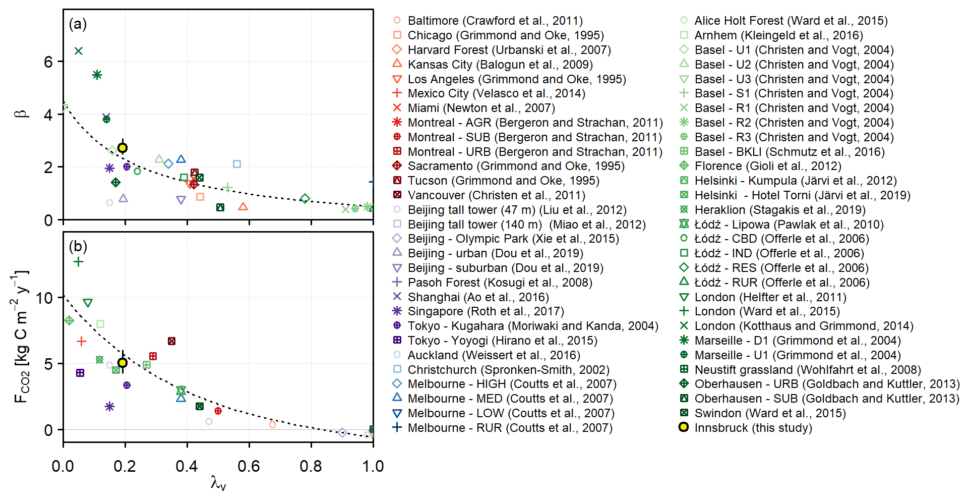
Figure 14(a) Daytime or midday (depending on which is given in the corresponding publication) Bowen ratio during summer and (b) annual net carbon flux versus vegetation fraction λv for IAO and for various sites in the literature (see the legend for references). Error bars for IAO indicate the spread of (a) daytime summertime values for the different years and (b) annual totals over the four 12-month periods of the dataset. The dotted lines in panel (a) are Eq. (3) from Christen and Vogt (2004) and in panel (b) from Nordbo et al. (2012).
At shorter timescales, however, the energy balance terms are impacted by Innsbruck's orographic setting. An interesting feature of observed QH at FLUG is the unusual shape of the diurnal cycle, particularly in April and May (Fig. 12g). Rather than peaking close to noon, QH peaks in the morning and then becomes appreciably negative in the afternoon, while QE remains large and positive until sunset. Close inspection of the time series reveals that this is largely a result of warm foehn air (i.e. warmer than the surface beneath) reaching FLUG in the afternoon (Fig. 8j; Sect. 5.4), and since foehn occurred frequently during Spring 2018, this pattern shows up in the monthly averages. However, similar behaviour is also seen on valley wind days (Fig. 6) and has been observed at other rural sites in the Inn Valley as well (Vergeiner and Dreiseitl, 1987; Babić et al., 2021; Lehner et al., 2021). At IAO, the much larger QH and smaller QE means that a similar change in the sign of QH during the afternoon is not seen, but QH does rise earlier in the day and peak first (just before or around solar noon), while QE reaches its maximum later in the day (after solar noon) and remains at moderate values until the evening. As a result, the diurnal cycle of the Bowen ratio at IAO is asymmetrical as is seen most clearly in summer (Fig. 12j).
The reason for this phase shift between QH and QE is not fully understood. Frequent afternoon thunderstorms seem to enhance QE during summer afternoons, but the trend remains if times with rain and shortly following rain are excluded. A larger vapour pressure deficit in the afternoons acting to increase QE could also be a contributing factor. Air temperature exceeding surface temperature during foehn (at both IAO and FLUG) or during the afternoon on some valley wind days (at FLUG) also plays a role. The behaviour does not appear to be related to differences in radiative input (since the shift between QH and QE is also seen in the ratio of the turbulent fluxes to Q*) or changing source area characteristics.
Due to the temporal patterns in wind direction at this complex-terrain site (Sect. 5.1), the source area itself varies systematically with time of day and season, being located west of IAO (with a slightly larger vegetation fraction, a larger proportion of water and a smaller building fraction) for down-valley winds during nighttime and winter months and east of IAO (towards the city centre) for up-valley winds during the daytime in summer. There is no clear evidence of spatial variations in energy partitioning as a result of surface cover variability around the site, although some variation with wind direction is observed as a result of differences in weather conditions (e.g. fair weather tends to coincide with daytime up-valley winds). The slightly higher vegetation fraction for down-valley winds is not large enough to generate a discernible increase in evaporative fluxes for this wind sector. Furthermore, the river, despite its proximity, does not provide a strong evaporative flux that is detected by the instruments. Similar results were found in central London, where a major river passes close to the measurement site yet appears not to contribute to the observed moisture flux (Kotthaus and Grimmond, 2014b). Perhaps an internal boundary layer forms over the river which does not reach the instrument height, or the low water temperature could limit evaporation (Sugawara and Narita, 2012).
The observed CO2 fluxes () at this city centre site are dominated by anthropogenic emissions. is positive throughout the day and all year round (Fig. 12k, v). Similar to other city centre sites (e.g. Nemitz et al., 2002; Björkegren and Grimmond, 2017; Järvi et al., 2019), the highest values are generally observed during the middle of the day, but the shape of the diurnal cycle at IAO varies throughout the year. In the winter months, the flux is slightly higher either side of midday and more closely resembles the typical double-peaked diurnal cycle often attributed to rush hour activities, while in summer the peak appears to be shifted towards the afternoon.
In contrast, there is clear photosynthetic uptake at the grassland site (FLUG) during the growing season (Fig. 12k). Here, daytime during spring and autumn follows a typical light-response curve when plotted against photosynthetically active radiation, PAR (Fig. 15a), estimated as a proportion (0.47) of K↓ (Papaioannou et al., 1993). At IAO there is little dependence of on PAR (for small PAR, the tendency for to increase as PAR increases is because both anthropogenic activity and K↓ are largest in the middle of the day). At FLUG, the increase in nighttime with temperature (Fig. 15b) suggests that soil respiration is responsible for increased emissions during nighttime in spring and autumn (Fig. 12k). At IAO, any contribution of soil respiration is minor. Indeed, the opposite behaviour is seen, and CO2 emissions decrease with increasing temperature as demand for building heating falls. Although anthropogenic emissions far outweigh any biogenic contributions to the observed CO2 fluxes, it is possible to identify biogenic signals in other gases at IAO (Karl et al., 2018; Kaser et al., 2022).
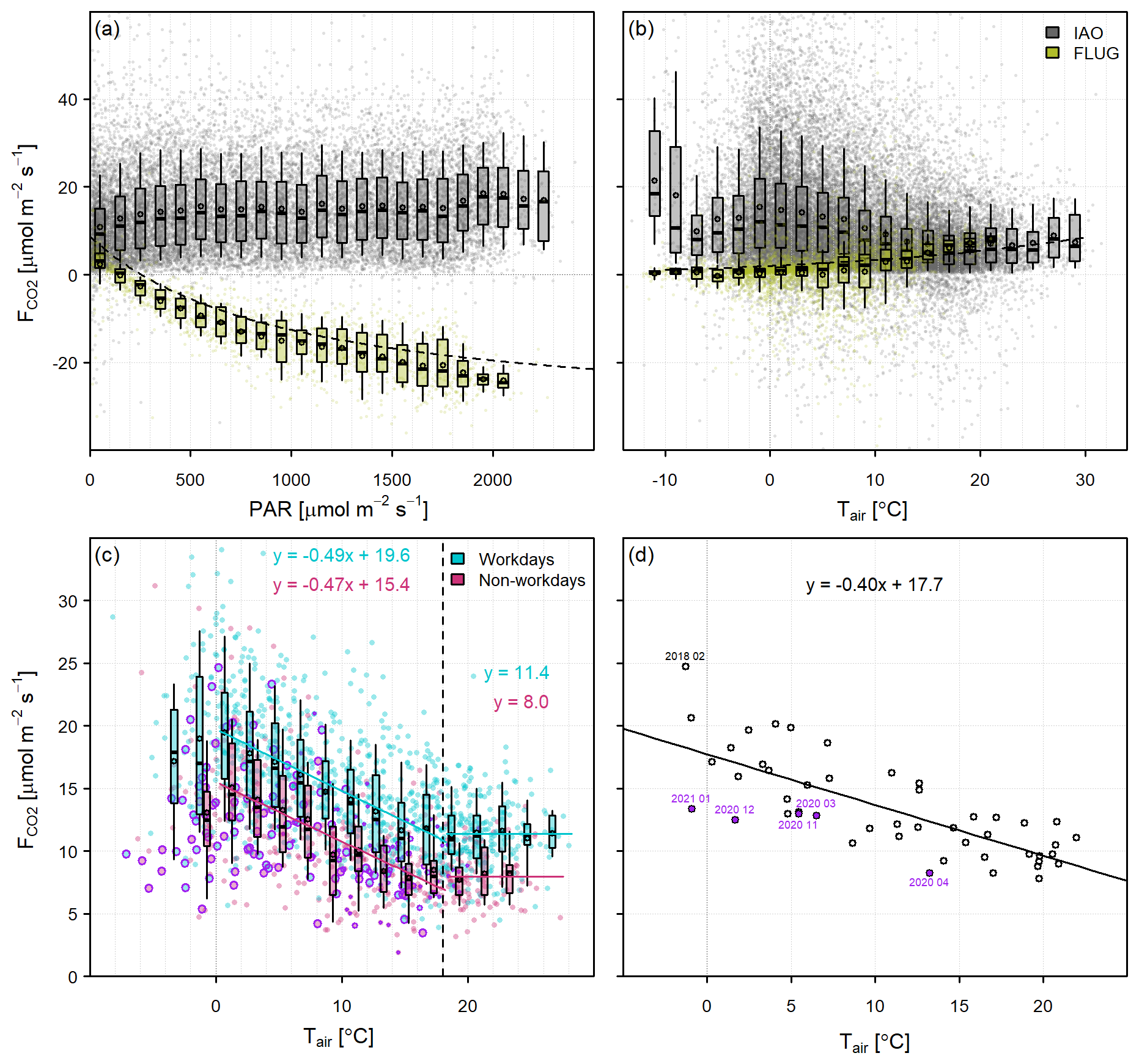
Figure 15(a) The 30 min daytime (K↓>5 W m−2) observed CO2 fluxes versus photosynthetically active radiation for all available data during the growing season (April–September, inclusive, but note that FLUG data are only available for 15 September 2017–22 May 2018), and (b) 30 min nighttime ( W m−2) observed CO2 fluxes versus air temperature for the urban (IAO) and grassland (FLUG) sites. The dashed lines show (a) the light-response curve and (b) soil respiration rate for a grassland site in the nearby Stubai Valley (Wohlfahrt et al., 2005; Li et al., 2008). (c) Daily mean CO2 flux versus daily mean air temperature separated into working and non-working days (daily values have been gap-filled using monthly median diurnal cycles for working and non-working days). Points outlined in purple occurred during COVID-19 restrictions. The vertical dashed line marks a base temperature of 18 ∘C, above which does not decrease with temperature. (d) Average monthly observed CO2 fluxes versus average monthly air temperature. Purple points indicate months with the strictest COVID-19 restrictions. In panels (a)–(c), boxes indicate the interquartile range, whiskers the 10th–90th percentile, horizontal bars the median and points the mean. In panels (c)–(d), solid lines are linear regressions with the equations given.
To further explore the anthropogenic controls on at IAO, the dependence on air temperature is shown at daily and monthly timescales in Fig. 15c–d. At the daily timescale, there is a clear linear decrease in with increasing temperature up to around 18 ∘C, above which remains constant. This type of behaviour suggests a substantial contribution of fuel combustion for building heating to observed (Sailor and Vasireddy, 2006; Bergeron and Strachan, 2011). On average, the data suggest that fuel combustion for space heating releases an extra 0.5 µmol m−2 s−1 CO2 for every 1 ∘C decrease in temperature, although this is thought to be an underestimate as the seasonal variability in amplitude is smaller than might be expected (see below). Assuming a negligible contribution from photosynthesis or soil respiration, the temperature-independent anthropogenic emissions amount to an average of 11.4 and 8.0 µmol m−2 s−1 on working and non-working days, respectively. These approximately temperature-independent emissions are attributed to human metabolism, fuel combustion for transport and fuel combustion in buildings that is not associated with space heating (e.g. for cooking or heating water).
The scatter seen in Fig. 15c arises from various factors, including the changing measurement source area, variability in human behaviour and the impact of weather conditions besides temperature (such as snow, rain or solar radiation affecting people's perception of temperature). The timing of unusually cool or warm spells affects energy consumption (e.g. a cold spell in September is likely associated with lower emissions than for the same temperature in December because people may not have switched on their heating yet). Similarly, high temperatures during foehn also contribute to deviations, particularly during winter (days with foehn tend to have higher emissions than would be expected given the temperature). Observed is higher on working days compared to non-working days by about 4 µmol m−2 s−1. Although working and non-working days have already been separated, emissions on Sundays tend to be lower than on Saturdays, and there is also some variability from Monday to Friday. During the COVID-19 restrictions, reduced emissions resulted in generally lower observed , particularly on working days (see also Lamprecht et al., 2021; Nicolini et al., 2022).
The temperature dependence of the building heating demand explains most of the monthly variation in observed (Fig. 15d; square of the correlation coefficient, r2=0.57). Reduced traffic during the periods with the strictest COVID-19 restrictions in March–April 2020 and November 2020–February 2021 means observed is also towards the bottom of the distribution for these months (see also Fig. 12v). The highest monthly was recorded for February 2018 and is considerably higher than expected, given the average monthly temperature. This is attributed to a period of very cold weather towards the end of the month (Fig. 3c) which coincided with easterly winds.
A marked difference in observed CO2 fluxes with wind direction is seen at IAO. Fluxes from the eastern sector (60–120∘) are about twice as high as those from the western sector (210–270∘). Monthly diurnal cycles are considered to avoid biases by season and by time of day (Fig. 16a, b), although easterly winds are still associated with more unstable conditions. Although the land cover composition is quite similar for these two main sectors (Sect. 3), the eastern sector is more densely built with a larger proportion of buildings and roads and busier roads (including a crossroads close to the site), whereas the western sector contains fewer roads, more widely spaced institutional buildings and more vegetation and water (Fig. 2). The observed data represent a combination of the spatiotemporally varying contributions of anthropogenic emissions, the variation in the flux footprint with season and with time of day and the level of turbulent mixing. The strong seasonal and diurnal dependence of wind direction (Sect. 5.1) must be considered when interpreting the dataset, as characteristic features arise from a mixture of temporal changes in sources and sinks combined with differences in spatial sampling due to the changing source area. For example, the shift in peak CO2 fluxes to the afternoon that is particularly evident in summer is likely due to the diurnal wind shifting from westerly (low emissions) to easterly (high emissions), since this asymmetry is neither seen in the diurnal cycles of western and eastern sectors (Fig. 16a), nor in the emissions modelled using a statistical inventory approach (analogous to the estimation of QF, Appendix B), which accounts for temporal variability in human activities but not spatial variability around the tower. Moreover, in winter, when westerly winds are more common, the observed data are more representative of the lower emissions from the western sector, whereas in summer the afternoon data are more representative of higher emissions from the eastern sector. This bias in source area sampling probably results in lower wintertime fluxes and higher summertime averages compared to if the observations were evenly representative of the source area. This leads to slightly smaller seasonal variation (and hence a weaker temperature dependence in Fig. 15c–d), as the higher emissions in winter are partly compensated by a greater frequency of westerly winds, leading to lower observed fluxes (and the opposite situation in summer). Additionally, the easterly winds during the period of cold weather in February 2018 further enhanced observed during this period compared to the source area average.
Figure 16(a, c) Monthly median diurnal cycles (shading indicates interquartile range) and (b, d) the corresponding daily mean fluxes by month for (a–b) observed carbon dioxide fluxes separated into eastern (60–120∘) and western (210–270∘) wind sectors and (c–d) observed and modelled carbon dioxide fluxes. In panel (d), the modelled emissions are separated into contributions from building heating (FCO2_B), traffic (FCO2_V) and human metabolism (FCO2_M).
Using median diurnal cycles to gap-fill the observations (Järvi et al., 2012) gives an annual total CO2 flux of 5.1 kg C m−2 yr−1 (varying between 4.3 and 6.0 kg C m−2 yr−1 for the four May-to-May 12-month periods in the study period). For comparison, the annual uptake at the nearby Neustift grassland site is 0.018 kg C m−2 yr−1 (Wohlfahrt et al., 2008). The annual CO2 flux at IAO is well within expectations, given the proportion of vegetation (Fig. 14b). Similar annual totals (4.9–5.6 kg C m−2 yr−1) and vegetation fractions (12 %–29 %) were found for Basel (Schmutz et al., 2016), Beijing (Liu et al., 2012), Helsinki (Järvi et al., 2019), Heraklion (Stagakis et al., 2019) and Montreal (Bergeron and Strachan, 2011). In Montreal, the annual total is higher than suggested by the vegetation fraction alone, possibly due to the cold climate (as is also the case for Vancouver; Christen et al., 2011), while in Heraklion, where space heating emissions are small, the annual total is lower. Considering the eastern and western sectors separately at IAO gives annual totals of 7.0 and 3.3 kg C m−2 yr−1, respectively (which rather fortuitously average to give 5.1 kg C m−2 yr−1, in agreement with the measured total given above). These values are also within the range suggested by previous studies if the proportion of vegetation and water in the source area is considered (10 %/28 % for the eastern/western sectors). Even a small amount of vegetation or open water can make a substantial difference to the emissions in city centres, as it is not only photosynthetic uptake by vegetation but also the absence of roads or buildings (which would contribute substantially to the emissions) associated with vegetated and water surfaces that is relevant.
Modelled CO2 emissions (Fig. 16b, d) result in a similar annual total of 5.0 kg C m−2 yr−1 and suggest that human metabolism accounts for 13 % of the annual total emissions, traffic 35 % and building energy use 53 %. However, these contributions vary considerably with time of year. On a daily basis, human metabolism contributes around 1.7 µmol m−2 s−1, fuel combustion for transport around 4.5 µmol m−2 s−1 and building energy use around 1.6 µmol m−2 s−1 in summer and 13 µmol m−2 s−1 in winter. In sum, daily total emissions are around 8 µmol m−2 s−1 in summer and 19 µmol m−2 s−1 in winter (Fig. 16d). The modelled emissions suggest working/non-working day differences are mainly due to traffic, but building energy use also contributes during winter. The reasonable agreement between modelled CO2 emissions and observed give confidence that the analogously calculated anthropogenic heat flux is an appropriate estimate for the study area. The model seems to overestimate emissions from building heating in winter (Fig. 16d), but this may partly result from the prevalence of westerly winds and associated underestimation of observed compared to the source area average. Future work will address the fine-scale spatial and temporal variability in emissions around the tower in more detail.
Having examined the climatology at IAO and explored the controls on the energy and carbon exchange, this section summarises the effects of complex terrain flows on near-surface conditions through comparison of valley wind days, foehn events and pre-foehn conditions. As has been shown above, although a twice-daily wind reversal is frequently observed in and around Innsbruck (Sect. 5.1), there are very few examples of purely thermally driven valley wind days. Similarly, many different types of foehn can occur with different characteristics, and there is often interaction with other types of flow. Given these complexities, a manual classification of different flow regimes was judged to be the most useful approach for the purposes of this analysis (see Appendix A for details).
While several case studies are presented above, Fig. 17 summarises the impact of the valley wind circulation, foehn events and pre-foehn conditions on near-surface conditions at IAO. Note that because the flow regimes occur under different synoptic conditions, the first two columns group data from different times of day (and times of year), while the third column helps to minimise the impact of diurnal and seasonal trends (although some lines are incomplete as the different regimes do not necessarily occur at all times in all seasons; for example, during winter nights pre-foehn is more common than foehn).
Figure 17Impact of different flow regimes (colours) on (a, k, u) turbulent kinetic energy, (b, l, v) wind speed, (c, m, w) gust speed, (d, n, x) air temperature, (e, o, y) the difference between surface and air temperature, (f, p, z) sensible heat flux, (g, q, A) sensible heat flux ratio, (h, r, B) latent heat flux, (I ,s, C) latent heat flux ratio and (j, t, D) CO2 mixing ratio at IAO. Box plots are shown for all data together (a–j) and for all data separated by month (k–t). Boxes indicate the interquartile range, whiskers the 10–90th percentiles and the median and mean are shown by horizontal bars and points, respectively. Median diurnal cycles (lines), interquartile ranges (dark shading) and 10–90th percentiles (light shading) are separated by season (u–D). The category “All” refers to the whole dataset (i.e. includes the other categories), and the proportion of the study period classified as each of the other categories is given above (a). Data are plotted if more than five data points are present.
During foehn, TKE and gust speeds are substantially higher than during non-foehn, highlighting that foehn is associated with intense turbulence and strong winds. TKE during foehn is typically between 4 and 9 m2 s−2, compared to days with a valley wind reversal when TKE reaches a maximum of 2–3 m2 s−2 during the up-valley flow (Fig. 17u). For pre-foehn conditions, wind speeds are comparable to those during foehn but TKE and gust speeds are lower (though still much higher than on valley wind days). Up-valley wind speeds often reach 2–4 m s−1 in spring and summer, slightly lower than median wind speeds during foehn, and down-valley winds are weak.
As valley wind days are driven by the heating of the valley atmosphere and often occur on fair-weather days, the amplitude of the diurnal cycles of Tair and Tsfc, as well as the difference Tsfc−Tair, is large, and particularly during the middle of the day, the surface is substantially warmer than the air (Fig. 17y). Valley wind days tend to have large positive QH which peaks early in the day (also evident in the ratio ; Fig. 17z, A). During foehn, the air temperature is substantially higher, especially during autumn and winter (Fig. 17n), and the diurnal cycle is much weaker (Fig. 17x) since nocturnal cooling is considerably reduced if foehn continues through the night (Figs. 7k, 8b, k). Enhanced Tair during foehn frequently (54 % of the time) exceeds the surface temperature and results in negative sensible heat fluxes (mainly in autumn and winter but also during the night in spring; Fig. 17p, z). In these cases, the influence of foehn overcomes the influence of the urban surface (which usually maintains positive QH). Only 9 % of QH data are negative at IAO, and 44 % of these occur during times classified as foehn or pre-foehn. Interestingly, pre-foehn conditions tend to have similarly low QH as for foehn conditions (compare similar times of day and times of year in Fig. 17z) despite lower air temperatures and a smaller temperature difference between surface and near-surface atmosphere. This may be a result of warm foehn air being brought down to the surface as the Inn Valley cold pool is eroded. Despite the high variability during foehn and pre-foehn, the effect of reduced QH during daytime and negative QH during nighttime can be seen in the ratio (Fig. 17A). For foehn conditions, daytime is slightly smaller in spring and autumn but much smaller in winter (0.2–0.4), and nighttime changes from around −0.5 to above 0.5 (as both QH and Q* are negative). There is some evidence for slightly enhanced latent heat fluxes at IAO during foehn compared to valley wind days (Fig. 17B, C), but this effect is minor (smaller than at FLUG), probably because of the lack of available water at IAO.
The intense mixing that accompanies foehn consistently maintains a low CO2 mixing ratio. The low values of observed during foehn are similar to those during daytime on valley wind days in spring and summer, with considerable thermal mixing and well-developed boundary layers (Fig. 17D). The dynamical mixing of foehn maintains low , also during the night, in contrast to nights following valley wind days when strong cooling and low wind speeds lead to high . Thus, foehn can be an important means of exchanging the air mass in the valley, particularly for urbanised valleys in autumn and winter when the trapping and buildup of emissions can be problematic. On the other hand, long-range transport and subsidence during foehn can increase the levels of other atmospheric constituents such as ozone (Seibert et al., 2000). There was no discernible impact of flow conditions on the observed net CO2 exchange, in accordance with Hiller et al. (2008), who measured CO2 fluxes from a grassland site in an Alpine valley and also concluded there were no obvious differences in the CO2 uptake observed during different wind regimes (foehn, valley wind and persistent up-valley wind).
Cities in mountainous terrain are subject to extreme and challenging conditions. For Innsbruck, heat stress in summer, heavy snowfall, road icing and avalanches in winter, flooding, downslope windstorms and air quality are all relevant issues. Understanding the underlying physical processes and their interactions is key to better predicting the occurrence, location and magnitude of such conditions. Moreover, knowledge of how cities in complex terrain are similar to and different from cities in flat terrain is crucial for avoiding inadvertent harmful effects that can result from attempts to mitigate climate issues. For such process studies (and for the evaluation of numerical models), direct measurement techniques such as eddy covariance are extremely valuable.
Here, 4 years of energy and carbon dioxide fluxes from the Alpine city of Innsbruck are presented and analysed. This study constitutes the first multi-year climatology of turbulence measurements from an urban area in highly complex terrain and reveals multiple ways in which Innsbruck's mountainous location impacts its meteorology. Fortunately for urban climatology and urban planners, many of the findings here are in accordance with previous urban studies.
-
Energy partitioning in Innsbruck is similar to that in other city centres. The considerable thermal mass of the urban surface stores a large amount of energy during the day and releases it at night.
-
Near-surface stable conditions are rare, as the release of stored heat and anthropogenic heat emissions maintain a positive sensible heat flux all day and all year round.
-
The low vegetation fraction around IAO keeps latent heat fluxes small and means there is very little opportunity for water to be stored. Water supplied to the surface through precipitation thus has an impact (on the energy balance and albedo) only for a short time (6–12 h) before it evaporates or is removed as runoff.
-
In good agreement with the urban literature, the proportion of vegetation is a reasonable predictor of the partitioning of energy between sensible and latent heat fluxes (in terms of the summer daytime Bowen ratio) and annual CO2 exchange.
-
The annual observed CO2 flux of 5.1 kg C m−2 yr−1 is dominated by anthropogenic emissions and is in reasonable agreement with emissions estimated from a statistical inventory approach (5.0 kg C m−2 yr−1), which suggests that traffic is the largest source of CO2 during summer and building heating in winter. Future work to develop a more advanced emissions model for Innsbruck will offer further insight.
However, Innsbruck's orographic setting and mountain weather affects near-surface conditions in multiple ways and gives rise to specific features.
-
The radiative fluxes are affected via orographic shading (incoming shortwave radiation is blocked by the terrain so that local sunrise/sunset is later/earlier than over flat terrain). On convective days with clear skies over the valley centre, cloud formation over the crests can further reduce incoming solar radiation during the late afternoon.
-
Atmospheric transmissivity is related to the composition of the valley atmosphere which can be high in aerosols (biogenic and anthropogenic pollutants), particularly during winter.
-
The thermally driven valley wind circulation in the Inn Valley gives rise to strong diurnal and seasonal cycles in flow and turbulence. In Innsbruck, the anabatic winds are stronger than the katabatic flow, and the strength and duration of the up-valley wind is greatest in spring and summer. In winter, weak down-valley flow dominates, and the up-valley period is either very short or does not occur at all.
-
These patterns complicate interpretation of local-scale measurements since the EC source area is biased towards particular wind sectors for certain conditions. Fortunately, the relatively homogenous source area of the IAO tower means the footprint composition does not change dramatically for different conditions. No clear differences in energy partitioning related to source area characteristics could be identified, but CO2 fluxes are considerably higher for the more densely built eastern sector with busier roads than for the western sector with more vegetation and open water. As a result, the observed CO2 fluxes likely underestimate the winter and overestimate the summer emissions compared to the neighbourhood average.
-
In spring and autumn, southerly foehn events have a marked impact on conditions in Innsbruck. High wind speeds and very large turbulent kinetic energies are observed, which help to disperse urban pollutants (shown here by very low CO2 mixing ratios).
-
The advection of warm air during foehn leads to negative sensible heat fluxes, even in the urban environment (and more often outside the urban area), especially in autumn and winter. The limited water availability appears to restrict QE in the urban environment compared to rural locations where enhanced QE is observed. Although QH can be strongly negative during foehn, these conditions are usually classified by the stability parameter, based on the Obukhov length, as neutral (not stable), since wind speeds are high.
-
The valley wind circulation also seems to be responsible for reduced QH and enhanced QE during the afternoons. This feature is most evident at rural sites with greater availability of water, where QH can turn negative long before sunset but also seems to reduce QH in the afternoons at IAO.
Since the local- and mesoscale circulations that occur in mountainous regions also occur to some extent over less complex terrain, and at great distances from the mountains, the results here are widely relevant, particularly for densely populated coastal cities also subject to strong seasonal and diurnal variation in circulation patterns. For the first time, this study describes the effects on urban surface–atmosphere exchange of a highly complex mountain setting using the IAO site located on the floor of the Inn Valley; future work should consider urban surfaces on sloping terrain.
A1 Identification of flow regime
To enable investigation of the impact different orographic flow regimes on surface–atmosphere exchange, the clearest examples of thermally dominated (i.e. valley wind) and dynamically dominated (i.e. foehn) events have been identified. In reality, there are few textbook cases of thermally driven or dynamically driven events; most days consist of a mixture of interacting processes across a wide range of scales. Hence, there are very few days that can be selected as examples of a purely thermally driven valley wind circulation (Lehner et al., 2019). Similarly, foehn events can vary considerably, and the beginning and end of breakthrough periods are not easy to classify (Mayr et al., 2018). It can also be difficult to distinguish foehn from pre-foehn (when conditions are strongly affected by foehn flow aloft but the foehn air does not reach the surface). Different flow regimes can give rise to similar temporal patterns in wind speed and direction. For instance, a breakthrough of foehn to the west of Innsbruck can appear similar to a thermally driven up-valley flow, especially if the breakthrough occurs in the afternoon, appears as easterly flow and coincides with increased wind speeds (e.g. as for FLUG in Fig. 8). The complexity of the situation makes automated classification extremely difficult. As it is not the intention here to develop algorithms that could be used more generally to classify different conditions, manual classification was found to be the most useful approach for facilitating the understanding of the observations at IAO and examining the impact of these different conditions on near-surface conditions.
A2 Valley wind days
Days with a transition from down-valley to up-valley flow and back again in both the Inn Valley and Wipp Valley, with no obvious foehn or other flow type, are designated valley wind days. The requirement for wind reversal also in the Wipp Valley largely eliminates days with foehn flow in the Wipp Valley (for which a continuous southerly wind is usually observed). However, days with weak synoptic forcing when a down-valley wind prevails in both valleys (common in winter) are missed when using this approach. Note that the requirement for a reversal to down-valley flow again was met if it happened shortly after midnight in the Inn Valley, as the up-valley period can last until late evening in summer (Fig. 5). The results would not change significantly if the algorithm of Lehner et al. (2019) had been used to select ideal valley wind (i.e. synoptically undisturbed clear-sky) days, but the manual classification includes many more days (and is not restricted to clear-sky conditions).
A3 Foehn events and pre-foehn conditions
As a prerequisite for both foehn and pre-foehn conditions in the Inn Valley, southerly foehn had to be present in the Wipp Valley (i.e. strong southerly winds at Steinach (S in Fig. 1) and high foehn probabilities, according to the statistical mixture model of Plavcan et al., 2014). Times when the foehn reached IAO were then judged from visual inspection of the time series, largely based on closely matched potential temperatures at IAO and Steinach, but changes in air temperature, relative humidity, wind speed and direction at IAO were also taken into account. Unclear events, non-southerly foehn and very short possible breakthroughs were ignored. Hence, not all foehn events are captured by this approach – but the majority of cases and the most clear-cut cases are. Comparison with the statistical foehn diagnosis algorithms of Plavcan et al. (2014) revealed good agreement in terms of diurnal and seasonal patterns, although the manual approach identifies slightly more cases in winter and nighttime. Disagreement between methods resulted from differences in availability of required input data, uncertainty about the timing of the onset and cessation of foehn (e.g. foehn ceases but the warm air mass remains) and differences between the approaches used (e.g. some of the statistical methods specify southerly wind directions, but deflected foehn can be from a range of directions in Innsbruck; see Sect. 5.4). The level of agreement and reasons for differences between methods are similar to those discussed between the various algorithms presented in Plavcan et al. (2014). Accounting for differences in data availability 95 % of the times identified as foehn by the manual approach are also diagnosed as foehn by the statistical algorithm that is not restricted by wind direction. The results would not change substantially if one of the foehn diagnoses of Plavcan et al. (2014) had been used instead of the manual approach. For the pre-foehn conditions, again southerly foehn had to be present in the Wipp Valley, but in contrast to a foehn breakthrough, the potential temperature at IAO is usually below the foehn temperature and strong westerly winds (pre-foehn westerlies) are often observed (Zängl, 2003).
A4 Identification of clear-sky days
Clear-sky days in Innsbruck were identified using time series plots of 1 min incoming shortwave (K↓) and longwave (L↓) radiation at IAO plus visual inspection of webcam images to clarify ambiguous cases. Days with perfectly smooth or almost perfectly smooth diurnal cycles of K↓ and L↓ were classified as clear-sky days at IAO (141 in total). This manual approach was found to be more useful than using thresholds (e.g. of K↓ relative to K↓ at the top of the atmosphere; K↓ TOA) due to several complicating factors. These include (i) substantial variability in atmospheric transmissivity even for cloud-free days (Fig. 10a), (ii) short thunderstorms and associated cloud cover which can develop in the late afternoon and do not dramatically affect daily , (iii) cumulus clouds forming above the peaks and ridges (Sect. 6.1) but not above the valley centre and (iv) some very high values despite mostly cloudy skies, which occur when the Sun shines through a gap in the clouds (observed K↓ is comprised of a large direct radiation component plus appreciable diffuse radiation).
Anthropogenic heat flux and associated carbon dioxide emissions were estimated for the study area following a conventional approach based on available statistics (e.g. Sailor and Lu, 2004) that combines contributions from energy use within buildings, traffic and human metabolism. It is beyond the scope of this study to develop a detailed emissions model for Innsbruck (this is planned in future); the aim here is to obtain a first-order estimation to provide context for the observational analysis. For this section, all times refer to local time (UTC+1 or UTC+2 during daylight saving time).
The average metabolic energy release per person was assumed to be 175 W m−2 cap−1 when awake and 75 W m−2 cap−1 when asleep (Sailor and Lu, 2004). People are assumed to be awake between 08:00 and 21:00 on working days and between 09:00 and21:00 on non-working days and asleep between 23:00 and 06:00 on working days and between 23:00 and 07:00 on non-working days. The population density on non-working days and during the night is 7000 km−2 for the centre of Innsbruck (City Population, 2018) and, based on the number of commuters (Statistik Austria, 2016), was estimated to increase by 25 % during working hours to 8800 km−2. Working hours are 08:00–16:00, and non-working hours are 18:00–06:00. During the transition times, population density and metabolic energy release were linearly interpolated. Multiplying these two quantities gave the anthropogenic heat flux due to human metabolism. For the corresponding CO2 release, emission factors of 280 µmol s−1 cap−1 and 120 µmol s−1 cap−1 were used for waking and sleeping hours, respectively (Moriwaki and Kanda, 2004).
Domestic energy consumption for the study area was downscaled from the total energy consumption for the Tirol region for 2015/2016 (Statistik Austria, 2017a) using population density. Energy consumption was available separated into contributions from different energy sources (e.g. electricity, oil, wood, district heating and gas) and for different purposes (classified as heating and non-heating purposes). All energy sources were assumed to contribute to the anthropogenic heat flux, whilst the CO2 emissions associated with electricity and district heating were assumed to occur outside the study area and thus were not included in the CO2 emissions estimated here. Although wood burning is still common in smaller towns and villages in Tirol, it is no longer used much in Innsbruck, so wood burning was apportioned to gas instead. Emission factors of g CO2 J−1 for oil and g CO2 J−1 for gas were used (IPCC, 2006). Daily energy use for non-heating purposes was assumed constant, whilst daily energy use for heating purposes was assumed to scale with heating degree days (Sailor and Vasireddy, 2006). An increase in energy use of 0.45 W m−2 K−1 was obtained using a base temperature of 18.3 ∘C (Sailor et al., 2015), which appears to be a reasonable threshold for Innsbruck, based on Fig. 15c. The daily values were then downscaled to 30 min using standard profiles of building energy use for working days and non-working days in Austria (Ghaemi and Brauner, 2009). Non-domestic building energy use is estimated as a proportion (0.42) of domestic building energy use, given that 26 %/11 % of the total building energy use in Europe is domestic/non-domestic (Pérez-Lombard et al., 2008). Non-domestic building energy use was assumed to be 70 % and 50 % of the working day value for Saturdays and for Sundays and holidays, respectively. Non-domestic energy use profiles from Hamilton et al. (2009) were used to downscale daily values to 30 min.
The total number of kilometres driven by passenger cars in Tirol in 2015/2016 (Statistik Austria, 2017b) was scaled by population density for the centre of Innsbruck to estimate the weight of traffic in the study area (contributions from motorcycles, public transport or goods transport are neglected in this approach). Hourly traffic count data for seven stations around Innsbruck for January 2018–June 2020 (provided by Amt der Tiroler Landesregierung, Abteilung Verkehrsplanung) were used to derive average traffic rates and median diurnal cycles for the following four groups: Mondays–Thursdays, Fridays, Saturdays and Sundays and holidays. Traffic rates on Fridays, Saturdays, and Sundays and holidays were about 105 %, 77 %, and 55 % of traffic rates on Mondays–Thursdays, respectively. Monthly traffic counts for the study period for the seven stations around Innsbruck (Land Tirol, 2020) were used to account for monthly and interannual variation in traffic rates across the whole study period (e.g. due to COVID-19 restrictions). From the average traffic weight (scaled according to month, type of day and time of day), the heat flux was calculated assuming an emission factor of 3.97 MJ km−1 per vehicle (Sailor and Lu, 2004). For CO2, an emission factor of 0.17 kg CO2 km−1 per vehicle was used (Statistik Austria, 2017b). The variation in the emission factor with speed and type of vehicles was neglected, as specific information was not available.
The Objective Hysteresis Model (OHM; Grimmond et al., 1991) estimates the net storage heat flux ΔQS from the net radiation Q* as follows:
where f is the proportion of each surface cover type i, are coefficients for each surface cover type, and t is time. The coefficients were taken from the literature (Table C1) and resulted in bulk values for 500 m around IAO of 0.475, 0.287 h and −33.1 W m−2 for a1, a2 and a3, respectively. Note that deriving bulk coefficients using observed Q* and ΔQS_RES showed little seasonal variation at IAO, in contrast to other studies (Anandakumar, 1999; Ward et al., 2016).
Table C1Coefficients for each surface type used in the Objective Hysteresis Model.
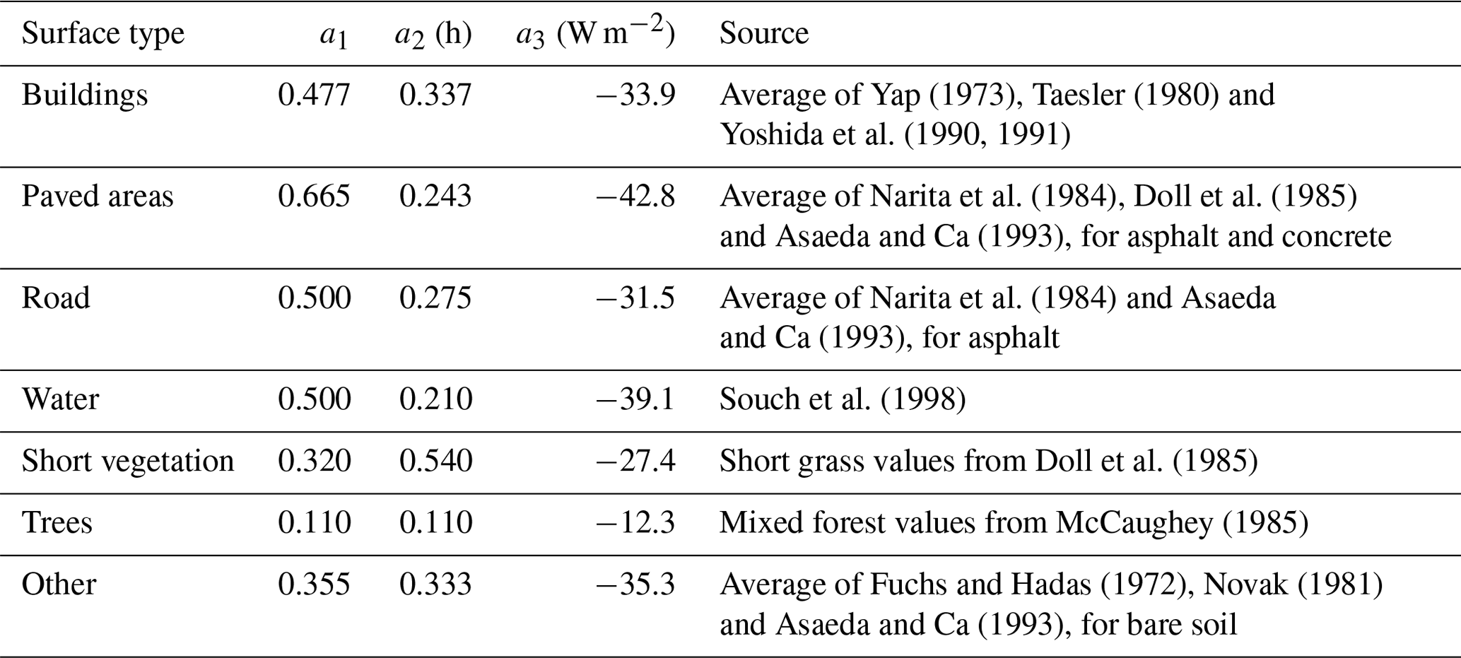
Data collected as part of the PIANO project are accessible via Zenodo at https://doi.org/10.5281/zenodo.4674773 (Gohm et al., 2021a), https://doi.org/10.5281/zenodo.4745957 (Gohm et al., 2021b) and https://doi.org/10.5281/zenodo.5795431 (Ward et al., 2021).
HCW and MWR designed the study. HCW conducted the analysis and prepared the paper, with contributions from all co-authors. All authors contributed to collection and processing of the various datasets involved.
At least one of the (co-)authors is a member of the editorial board of Atmospheric Chemistry and Physics. The peer-review process was guided by an independent editor, and the authors also have no other competing interests to declare.
Publisher’s note: Copernicus Publications remains neutral with regard to jurisdictional claims in published maps and institutional affiliations.
This work has been funded by the Austrian Science Fund (FWF) Lise Meitner programme (grant no. M2244-N32) and a research stipend from Innsbruck University. Observations at IAO are possible thanks to Hochschulraum-Strukturmittel funds provided by the Austrian Federal Ministry of Education, Science and Research, and the European Commission Seventh Framework (ALP-AIR; grant no. 334084). Research at IAO is also supported by FWF (grant nos. P30600-NBL and P33701-N). Part of the data collection and analysis were undertaken within the framework of the PIANO project supported by the FWF and the Weiss Science Foundation (grant no. P29746-N32). We thank Florian Haidacher (Amt der Tiroler Landesregierung, Abteilung Mobilitätsplanung), for providing the official traffic data referenced in this study.
This research has been supported by the Austrian Science Fund (grant nos. M2244-N32, P29746-N32, P30600-NBL and P33701-N), the Austrian Federal Ministry of Education, Science and Research and the European Commission Seventh Framework (grant no. 334084).
This paper was edited by Christoph Gerbig and reviewed by two anonymous referees.
Adler, B., Kalthoff, N., and Kiseleva, O.: Detection of structures in the horizontal wind field over complex terrain using coplanar Doppler lidar scans, Meteorol. Z., 29, 467–481, https://doi.org/10.1127/metz/2020/1031, 2020.
Allwine, K. J., Shinn, J. H., Streit, G. E., Clawson, K. L., and Brown, M.: Overview of URBAN 2000: A Multiscale Field Study of Dispersion through an Urban Environment, Bull. Am. Meteorol. Soc., 83, 521–536 https://doi.org/10.1175/1520-0477(2002)083<0521:OOUAMF>2.3.CO;2, 2002.
Anandakumar, K.: A study on the partition of net radiation into heat fluxes on a dry asphalt surface, Atmos. Environ., 33, 3911–3918, 1999.
Ao, X., Grimmond, C. S. B., Chang, Y., Liu, D., Tang, Y., Hu, P., Wang, Y., Zou, J., and Tan, J: Heat, water and carbon exchanges in the tall megacity of Shanghai: challenges and results, Int. J. Climatol., 36, 4608–4624, https://doi.org/10.1002/joc.4657, 2016.
Asaeda, T. and Ca, V.: The subsurface transport of heat and moisture and its effect on the environment: A numerical model, Bound.-Lay. Meteorol., 65, 159–179, https://doi.org/10.1007/BF00708822, 1993.
Babić, N., Adler, B., Gohm, A., Kalthoff, N., Haid, M., Lehner, M., Ladstätter, P., and Rotach, M. W.: Cross-valley vortices in the Inn valley, Austria: Structure, evolution and governing force imbalances, Q. J. Roy. Meteorol. Soc., 147, 3835–3861, https://doi.org/10.1002/qj.4159, 2021.
Balogun, A., Adegoke, J., Vezhapparambu, S., Mauder, M., McFadden, J., and Gallo, K.: Surface energy balance measurements above an exurban residential neighbourhood of Kansas City, Missouri, Bound.-Lay. Meteorol., 133, 299–321, https://doi.org/10.1007/s10546-009-9421-3, 2009.
Bergeron, O. and Strachan, I. B.: Wintertime radiation and energy budget along an urbanization gradient in Montreal, Can. Int. J. Climatol., 32, 137–152, https://doi.org/10.1002/joc.2246, 2010.
Bergeron, O. and Strachan, I. B.: CO2 sources and sinks in urban and suburban areas of a northern mid-latitude city, Atmos. Environ., 45, 1564–1573, https://doi.org/10.1016/j.atmosenv.2010.12.043, 2011.
Björkegren, A. and Grimmond, C. S. B.: Net carbon dioxide emissions from central London, Urban Clim., 23, 131–158, https://doi.org/10.1016/j.uclim.2016.10.002, 2017.
Christen, A. and Vogt, R.: Energy and radiation balance of a central European city, Int. J. Climatol., 24, 1395–1421, https://doi.org/10.1002/joc.1074, 2004.
Christen, A., Rotach, M. W., and Vogt, R.: The Budget of Turbulent Kinetic Energy in the Urban Roughness Sublayer, Bound.-Lay. Meteorol., 131, 193–222, https://doi.org/10.1007/s10546-009-9359-5, 2009.
Christen, A., Coops, N., Crawford, B., Kellett, R., Liss, K., Olchovski, I., Tooke, T., Van Der Laan, M., and Voogt, J.: Validation of modeled carbon-dioxide emissions from an urban neighborhood with direct eddy-covariance measurements, Atmos. Environ., 45, 6057–6069, https://doi.org/10.1016/j.atmosenv.2011.07.040, 2011.
City Population: Population of Innsbruck by quarter, https://www.citypopulation.de/php/austria-innsbruck.php (last access: 20 March 2019), 2018.
Coutts, A. M., Beringer, J., and Tapper, N. J.: Characteristics influencing the variability of urban CO2 fluxes in Melbourne, Australia, Atmos. Environ., 41, 51–62, https://doi.org/10.1016/j.atmosenv.2006.08.030, 2007a.
Coutts, A. M., Beringer, J., and Tapper, N. J.: Impact of increasing urban density on local climate: Spatial and temporal variations in the surface energy balance in Melbourne, Australia, J. Appl. Meteorol. Climatol., 46, 477–493, https://doi.org/10.1175/jam2462.1, 2007b.
Crawford, B., Grimmond, C. S. B., and Christen, A.: Five years of carbon dioxide fluxes measurements in a highly vegetated suburban area, Atmos. Environ., 45, 896–905, https://doi.org/10.1016/j.atmosenv.2010.11.017, 2011.
Crawford, B., Krayenhoff, E. S., and Cordy, P.: The urban energy balance of a lightweight low-rise neighborhood in Andacollo, Chile, Theor. Appl. Climatol., 131, 55–68, https://doi.org/10.1007/s00704-016-1922-7, 2016.
Deventer, M. J., von der Heyden, L., Lamprecht, C., Graus, M., Karl, T., and Held, A.: Aerosol particles during the Innsbruck Air Quality Study (INNAQS): Fluxes of nucleation to accumulation mode particles in relation to selective urban tracers, Atmos. Environ., 190, 376–388, https://doi.org/10.1016/j.atmosenv.2018.04.043, 2018.
Doll, D., Ching, J. K. S., and Kaneshiro, J.: Parameterization of subsurface heating for soil and concrete using net radiation data, Bound.-Lay. Meteorol., 32, 351–372, https://doi.org/10.1007/BF00122000, 1985.
Doran, J. C., Fast, J. D., and Horel, J.: The VTMX 2000 campaign, Bull. Am. Meteorol. Soc., 83, 537–551, https://doi.org/10.1175/1520-0477(2002)083<0537:TVC>2.3.CO;2, 2002.
Dou, J., Grimmond, S., Cheng, Z., Miao, S., Feng, D., and Liao, M.: Summertime surface energy balance fluxes at two Beijing sites, Int. J. Climatol., 39, 2793–2810, https://doi.org/10.1002/joc.5989, 2019.
Dreiseitl, E., Feichter, H., Pichler, H., Steinacker, R., and Vergeiner, I.: Windregimes an der Gabelung zweier Alpentäler, Arch. Meteorol., Geophys. Bioklimatol. Ser. B, 28, 257–275, https://doi.org/10.1007/BF02245357, 1980.
Fernando, H. J. S.: Fluid Dynamics of Urban Atmospheres in Complex Terrain, Annu. Rev. Fluid Mech., 42, 365–389, https://doi.org/10.1146/annurev-fluid-121108-145459, 2010.
Foken, T. and Wichura, B.: Tools for quality assessment of surface-based flux measurements, Agr. Forest Meteorol., 78, 83–105, https://doi.org/10.1016/0168-1923(95)02248-1, 1996.
Fortuniak, K., Pawlak, W., and Siedlecki, M.: Integral Turbulence Statistics Over a Central European City Centre, Bound.-Lay. Meteorol., 146, 257–276, https://doi.org/10.1007/s10546-012-9762-1, 2013.
Fratini, G., Ibrom, A., Arriga, N., Burba, G., and Papale, D.: Relative humidity effects on water vapour fluxes measured with closed-path eddy-covariance systems with short sampling lines, Agr. Forest Meteorol., 165, 53–63, https://doi.org/10.1016/j.agrformet.2012.05.018, 2012.
Frey, C. M., Parlow, E., Vogt, R., Harhash, M., and Abdel Wahab, M. M.: Flux measurements in Cairo, Part 1: in situ measurements and their applicability for comparison with satellite data, Int. J. Climatol., 31, 218–231, https://doi.org/10.1002/joc.2140, 2011.
Fuchs, M. and Hadas, A.: The heat flux density in a non-homogeneous bare loessial soil, Bound.-Lay. Meteorol., 3, 191–200, https://doi.org/10.1007/BF02033918, 1972.
Ghaemi, S. and Brauner, G.: User behavior and patterns of electricity use for energy saving, Internationale Energiewirtschaftstagung an der TU Wien, IEWT, https://publik.tuwien.ac.at/files/PubDat_180870.pdf (last access: 29 March 2019), 2009.
Gioli, B., Toscano, P., Lugato, E., Matese, A., Miglietta, F., Zaldei, A., and Vaccari, F.: Methane and carbon dioxide fluxes and source partitioning in urban areas: The case study of Florence, Italy, Environ. Pollut., 164, 125–131, https://doi.org/10.1016/j.envpol.2012.01.019, 2012.
Giovannini, L., Zardi, D., de Franceschi, M., and Chen, F.: Numerical simulations of boundary-layer processes and urban-induced alterations in an Alpine valley, Int. J. Climatol., 34, 1111–1131, https://doi.org/10.1002/joc.3750, 2014.
Giovannini, L., Laiti, L., Serafin, S., and Zardi, D.: The thermally driven diurnal wind system of the Adige Valley in the Italian Alps, Q. J. Roy. Meteorol. Soc., 143, 2389–2402, https://doi.org/10.1002/qj.3092, 2017.
Gohm, A., Harnisch, F., Vergeiner, J., Obleitner, F., Schnitzhofer, R., Hansel, A., Fix, A., Neininger, B., Emeis, S., and Schäfer, K.: Air Pollution Transport in an Alpine Valley: Results From Airborne and Ground-Based Observations, Bound.-Lay. Meteorol., 131, 441–463, https://doi.org/10.1007/s10546-009-9371-9, 2009.
Gohm, A., Haid, M., Umek, L., Ward, H. C., and Rotach, M. W.: PIANO (Penetration and Interruption of Alpine Foehn) – Doppler wind lidar data set, Zenodo [data set], https://doi.org/10.5281/zenodo.4674773, 2021a.
Gohm, A., Umek, L., Haid, M., Ward, H. C., and Rotach, M. W.: PIANO (Penetration and Interruption of Alpine Foehn) – MOMAA weather station data set, Zenodo [data set], https://doi.org/10.5281/zenodo.4745957, 2021b.
Goldbach, A. and Kuttler, W.: Quantification of turbulent heat fluxes for adaptation strategies within urban planning, Int. J. Climatol., 33, 143–159, https://doi.org/10.1002/joc.3437, 2013.
Grimmond, C. S. B. and Oke, T. R.: Comparison of Heat Fluxes from Summertime Observations in the Suburbs of Four North American Cities, J. Appl. Meteorol., 34, 873–889, https://doi.org/10.1175/1520-0450(1995)034<0873:COHFFS>2.0.CO;2, 1995.
Grimmond, C. S. B. and Oke, T. R.: Aerodynamic properties of urban areas derived from analysis of surface form, J. Appl. Meteorol., 38, 1262–1292, https://doi.org/10.1175/1520-0450(1999)038<1262:APOUAD>2.0.CO;2, 1999.
Grimmond, C. S. B. and Oke, T. R.: Turbulent heat fluxes in urban areas: Observations and a local-scale urban meteorological parameterization scheme (LUMPS), J. Appl. Meteorol., 41, 792–810, https://doi.org/10.1175/1520-0450(2002)041<0792:THFIUA>2.0.CO;2, 2002.
Grimmond, C. S. B., Cleugh, H. A., and Oke, T. R.: An objective urban heat storage model and its comparison with other schemes, Atmos. Environ. Pt. B., 25, 311–326, 1991.
Grimmond, C. S. B., Salmond, J. A., Oke, T. R., Offerle, B., and Lemonsu, A.: Flux and turbulence measurements at a densely built-up site in Marseille: Heat, mass (water and carbon dioxide), and momentum, J. Geophys. Res.-Atmos., 109, D24101, D2410110.1029/2004jd004936, 2004.
Haid, M., Gohm, A., Umek, L., Ward, H. C., Muschinski, T., Lehner, L., and Rotach, M. W.: Foehn–cold pool interactions in the Inn Valley during PIANO IOP2, Q. J. Roy. Meteorol. Soc., 146, 1232–1263, https://doi.org/10.1002/qj.3735, 2020.
Haid, M., Gohm, A., Umek, L., Ward, H. C., and Rotach, M. W.: Cold-air pool processes in the Inn Valley during foehn: A comparison of four cases during PIANO, Bound.-Lay. Meteorol., 182, 335–362, https://doi.org/10.1007/s10546-021-00663-9, 2021.
Hamilton, I. G., Davies, M., Steadman, P., Stone, A., Ridley, I., and Evans, S.: The significance of the anthropogenic heat emissions of London's buildings: A comparison against captured shortwave solar radiation, Build. Environ., 44, 807–817, https://doi.org/10.1016/j.buildenv.2008.05.024, 2009.
Hammerle, A., Haslwanter, A., Tappeiner, U., Cernusca, A., and Wohlfahrt, G.: Leaf area controls on energy partitioning of a temperate mountain grassland, Biogeosciences, 5, 421–431 https://doi.org/10.5194/bg-5-421-2008, 2008.
Hayashi, M., Hirota, T., Iwata, Y., and Takayabu, I.: Snowmelt Energy Balance and Its Relation to Foehn Events in Tokachi, Japan, J. Meteorol. Soc. Jpn. Ser. II, 83, 783–798, https://doi.org/10.2151/jmsj.83.783, 2005.
Helfter, C., Famulari, D., Phillips, G. J., Barlow, J. F., Wood, C. R., Grimmond, C. S. B., and Nemitz, E.: Controls of carbon dioxide concentrations and fluxes above central London, Atmos. Chem. Phys., 11, 1913–1928, https://doi.org/10.5194/acp-11-1913-2011, 2011.
Henao, J. J., Rendón, A. M., and Salazar, J. F.: Trade-off between urban heat island mitigation and air quality in urban valleys, Urban Clim., 31, 100542, https://doi.org/10.1016/j.uclim.2019.100542, 2020.
Hiller, R., Zeeman, M. J., and Eugster, W.: Eddy-covariance flux measurements in the complex terrain of an Alpine valley in Switzerland, Bound.-Lay. Meteorol., 127, 449–467, https://doi.org/10.1007/s10546-008-9267-0, 2008.
Hirano, T., Sugawara, H., Murayama, S., and Kondo, H.: Diurnal variation of CO2 flux in an urban area of Tokyo, Sola, 11, 100–103, https://doi.org/10.2151/sola.2015-024, 2015.
Hirsch, A. L., Evans, J. P., Thomas, C., Conroy, B., Hart, M. A., Lipson, M., and Ertler, W.: Resolving the influence of local flows on urban heat amplification during heatwaves, Environ. Res. Lett., 16, 064066, https://doi.org/10.1088/1748-9326/ac0377, 2021.
Ichinose, T., Shimodozono, K., and Hanaki, K.: Impact of anthropogenic heat on urban climate in Tokyo, Atmos. Environ., 33, 3897–3909, https://doi.org/10.1016/S1352-2310(99)00132-6, 1999.
IPCC: 2006 IPCC guidelines for national greenhouse gas inventories, Institute for Global Environmental Strategies (IGES), ISBN 4-88788-032-4, 2006
Järvi, L., Nordbo, A., Junninen, H., Riikonen, A., Moilanen, J., Nikinmaa, E., and Vesala, T.: Seasonal and annual variation of carbon dioxide surface fluxes in Helsinki, Finland, in 2006–2010, Atmos. Chem. Phys., 12, 8475–8489, https://doi.org/10.5194/acp-12-8475-2012, 2012.
Järvi, L., Grimmond, C. S. B., Taka, M., Nordbo, A., Setälä, H., and Strachan, I. B.: Development of the Surface Urban Energy and Water Balance Scheme (SUEWS) for cold climate cities, Geosci. Model Dev., 7, 1691–1711, https://doi.org/10.5194/gmd-7-1691-2014, 2014.
Järvi, L., Rannik, Ü., Kokkonen, T. V., Kurppa, M., Karppinen, A., Kouznetsov, R. D., Rantala, P., Vesala, T., and Wood, C. R.: Uncertainty of eddy covariance flux measurements over an urban area based on two towers, Atmos. Meas. Tech., 11, 5421–5438, https://doi.org/10.5194/amt-11-5421-2018, 2018.
Järvi, L., Havu, M., Ward, H. C., Bellucco, V., McFadden, J. P., Toivonen, T., Heikinheimo, V. , Kolari, P., Riikonen, A., and Grimmond, C. S. B.: Spatial modelling of local-scale biogenic and anthropogenic carbon dioxide emissions in Helsinki, J. Geophys. Res.-Atmos., 124, 8363–8384, https://doi.org/10.1029/2018JD029576, 2019.
Jáuregui, E. and Luyando, E.: Global radiation attenuation by air pollution and its effects on the thermal climate in Mexico City, Int. J. Climatol., 19, 683–694, https://doi.org/10.1002/(SICI)1097-0088(199905)19:6<683::AID-JOC389>3.0.CO;2-8, 1999.
Johnson, G. T. and Watson, I. D.: The Determination of View-Factors in Urban Canyons, J. Appl. Meteorol. Climatol., 23, 329–335, https://doi.org/10.1175/1520-0450(1984)023<0329:tdovfi>2.0.co;2, 1984.
Karl, T., Graus, M., Striednig, M., Lamprecht, C., Hammerle, A., Wohlfahrt, G., Held, A., von der Heyden, L., Deventer, M. J., Krismer, A., Haun, C., Feichter, R., and Lee, J.: Urban eddy covariance measurements reveal significant missing NOx emissions in Central Europe, Sci. Rep., 7, 2536, https://doi.org/10.1038/s41598-017-02699-9, 2017.
Karl, T., Striednig, M., Graus, M., Hammerle, A., and Wohlfahrt, G.: Urban flux measurements reveal a large pool of oxygenated volatile organic compound emissions, P. Natl. Acad. Sci. USA, 115, 1186–1191, https://doi.org/10.1073/pnas.1714715115, 2018.
Karl, T., Gohm, A., Rotach, M. W., Ward, H. C., Graus, M., Cede, A., Wohlfahrt, G., Hammerle, A., Haid, M., Tiefengraber, M., Lamprecht, C., Vergeiner, J., Kreuter, A., Wagner, J., and Staudinger, M.: Studying urban climate and air quality in the Alps – The Innsbruck Atmospheric Observatory, Bull. Am. Meteorol. Soc., 101, E488–E507, https://doi.org/10.1175/BAMS-D-19-0270.1, 2020.
Karsisto, P., Fortelius, C., Demuzere, M., Grimmond, C. S. B., Oleson, K. W., Kouznetsov, R., Masson, V., and Järvi, L.: Seasonal surface urban energy balance and wintertime stability simulated using three land-surface models in the high-latitude city Helsinki, Q. J. Roy. Meteorol. Soc., 142, 401–417, https://doi.org/10.1002/qj.2659, 2015.
Kaser, L., Peron, A., Graus, M., Striednig, M., Wohlfahrt, G., Juráň, S., and Karl, T.: Interannual variability of terpenoid emissions in an alpine city, Atmos. Chem. Phys., 22, 5603–5618, https://doi.org/10.5194/acp-22-5603-2022, 2022.
Kleingeld, E., van Hove, B., Elbers, J., and Jacobs, C.: Carbon dioxide fluxes in the city centre of Arnhem, A middle-sized Dutch city, Urban Clim., 24, 994–1010, https://doi.org/10.1016/j.uclim.2017.12.003, 2018.
Kljun, N., Calanca, P., Rotach, M. W., and Schmid, H. P.: A simple two-dimensional parameterisation for Flux Footprint Prediction (FFP), Geosci. Model Dev., 8, 3695–3713, https://doi.org/10.5194/gmd-8-3695-2015, 2015.
Kordowski, K. and Kuttler, W.: Carbon dioxide fluxes over an urban park area, Atmos. Environ., 44, 2722–2730, https://doi.org/10.1016/j.atmosenv.2010.04.039, 2010.
Kosugi, Y., Takanashi, S., Ohkubo, S., Matsuo, N., Tani, M., Mitani, T., Tsutsumi, D., and Nik, A. R.: CO2 exchange of a tropical rainforest at Pasoh in Peninsular Malaysia, Agr. Forest Meteorol., 148, 439–452, https://doi.org/10.1016/j.agrformet.2007.10.007, 2008.
Kotthaus, S. and Grimmond, C. S. B.: Energy exchange in a dense urban environment – Part I: temporal variability of long-term observations in central London, Urban Clim., 10, 261–280, https://doi.org/10.1016/j.uclim.2013.10.002, 2014a.
Kotthaus, S. and Grimmond, C. S. B.: Energy exchange in a dense urban environment – Part II: impact of spatial heterogeneity of the surface, Urban Clim., 10, 281–307, https://doi.org/10.1016/j.uclim.2013.10.001, 2014b.
Lamprecht, C., Graus, M., Striednig, M., Stichaner, M., and Karl, T.: Decoupling of urban CO2 and air pollutant emission reductions during the European SARS-CoV-2 lockdown, Atmos. Chem. Phys., 21, 3091–3102, https://doi.org/10.5194/acp-21-3091-2021, 2021.
Land Tirol: Verkehrsinformation, https://verkehrsinformation.tirol.gv.at/web/html/vde.html#, last access: 22 February 2022.
Largeron, Y. and Staquet, C.: The Atmospheric Boundary Layer during Wintertime Persistent Inversions in the Grenoble Valleys, Front. Earth Sci., 4, 70, https://doi.org/10.3389/feart.2016.00070, 2016.
Lee, K., Hong, J. W., Kim, J., Jo, S., and Hong, J.: Traces of urban forest in temperature and CO2 signals in monsoon East Asia, Atmos. Chem. Phys., 21, 17833–17853, https://doi.org/10.5194/acp-21-17833-2021, 2021.
Lehner, M. and Rotach, M. W.: Current Challenges in Understanding and Predicting Transport and Exchange in the Atmosphere over Mountainous Terrain, Atmosphere, 9, 276, https://doi.org/10.3390/atmos9070276, 2018.
Lehner, M., Rotach, M. W., and Obleitner, F.: A Method to Identify Synoptically Undisturbed, Clear-Sky Conditions for Valley-Wind Analysis, Bound.-Lay. Meteorol., 173, 435–450, https://doi.org/10.1007/s10546-019-00471-2, 2019.
Lehner, M., Rotach, M. W., Sfyri, E., and Obleitner, F.: Spatial and temporal variations in near-surface energy fluxes in an Alpine valley under synoptically undisturbed and clear-sky conditions, Q. J. Roy. Meteorol. Soc., 147, 2173–2196, https://doi.org/10.1002/qj.4016, 2021.
Leukauf, D., Gohm, A., and Rotach, M. W.: Toward Generalizing the Impact of Surface Heating, Stratification, and Terrain Geometry on the Daytime Heat Export from an Idealized Valley, J. Appl. Meteorol. Climatol., 56, 2711–2727, https://doi.org/10.1175/jamc-d-16-0378.1, 2017.
Li, Y.-L., Tenhunen, J., Owen, K., Schmitt, M., Bahn, M., Droesler, M., Otieno, D., Schmidt, M., Gruenwald, T., Hussain, M. Z., Mirzae, H., and Bernhofer, C.: Patterns in CO2 gas exchange capacity of grassland ecosystems in the Alps, Agr. Forest Meteorol., 148, 51–68, https://doi.org/10.1016/j.agrformet.2007.09.002, 2008.
Liu, H., Feng, J., Järvi, L., and Vesala, T.: Four-year (2006–2009) eddy covariance measurements of CO2 flux over an urban area in Beijing, Atmos. Chem. Phys., 12, 7881–7892, https://doi.org/10.5194/acp-12-7881-2012, 2012.
MacDonald, M. K., Pomeroy, J. W., and Essery, R. L. H.: Water and energy fluxes over northern prairies as affected by chinook winds and winter precipitation, Agr. Forest Meteorol., 248, 372–385, https://doi.org/10.1016/j.agrformet.2017.10.025, 2018.
Matzinger, N., Andretta, M., Gorsel, E. V., Vogt, R., Ohmura, A., and Rotach, M. W.: Surface radiation budget in an Alpine valley, Q. J. Roy. Meteorol. Soc., 129, 877–895, https://doi.org/10.1256/qj.02.44, 2003.
Mayr, G. J., Armi, L., Arnold, S., Banta, R. M., Darby, L. S., Durran, D. D., Flamant, D., Gaberšek, S., Gohm, A., Mayr, R., Mobbs, S., Nance, L. B., Vergeiner, I., Vergeiner, J., and Whiteman, C. D.: Gap flow measurements during the Mesoscale Alpine Programme, Meteorol. Atmos. Phys., 86, 99–119, https://doi.org/10.1007/s00703-003-0022-2, 2004.
Mayr, G., Plavcan, D., Armi, L., Elvidge, A., Grisogono, B., Horvath, K., Jackson, P., Neururer, A., Seibert, P., Steenburgh, J. W., Stiperski, I., Sturman, A., Večenaj, Ž., Vergeiner, J., Vosper, S., and Zängl, G.: The Community Foehn Classification Experiment, Bull. Am. Meteorol. Soc., 99, 2229–2235, https://doi.org/10.1175/bams-d-17-0200.1, 2018.
McCaughey, J. H.: Energy balance storage terms in a mature mixed forest at Petawawa, Ontario – A case study, Bound.-Lay. Meteorol., 31, 89–101, https://doi.org/10.1007/BF00120036, 1985.
Miao, S., Chen, F., LeMone, M. A., Tewari, M., Li, Q., and Wang, Y.: An Observational and Modeling Study of Characteristics of Urban Heat Island and Boundary Layer Structures in Beijing, J. Appl. Meteorol. Climatol., 48, 484–501, https://doi.org/10.1175/2008JAMC1909.1, 2009.
Miao, S., Dou, J., Chen, F., Li, J., and Li, A.: Analysis of observations on the urban surface energy balance in Beijing, Sci. China Earth Sci., 55, 1881–1890, https://doi.org/10.1007/s11430-012-4411-6, 2012.
Moncrieff, J. B., Clement, R., Finnigan, J. J., and Meyers, T.: Averaging, detrending and filtering of eddy covariance time series, in: Handbook of Micrometeorology: a guide for surface flux measurements, edited by: Lee, X., Massman, W. J., and Law, B. E., Springer, Dordrecht, https://doi.org/10.1007/1-4020-2265-4_2, 2004.
Moriwaki, R. and Kanda, M.: Seasonal and diurnal fluxes of radiation, heat, water vapor, and carbon dioxide over a suburban area, J. Appl. Meteorol., 43, 1700–1710, https://doi.org/10.1175/JAM2153.1, 2004.
Muschinski, T., Gohm, A., Haid, M., Umek, L., and Ward, H. C.: Spatial heterogeneity of the Inn Valley Cold Air Pool during south foehn: Observations from an array of temperature, Meteorol. Z., 30, 153–168, https://doi.org/10.1127/metz/2020/1043, 2021.
Nadeau, D. F., Pardyjak, E. R., Higgins, C. W., Huwald, H., and Parlange, M. B.: Flow during the evening transition over steep Alpine slopes, Q. J. Roy. Meteorol. Soc., 139, 607–624, https://doi.org/10.1002/qj.1985, 2013.
Narita, K., Sekine, T., and Tokuoka, T.: Thermal properties of urban surface materials – study on heat balance at asphalt pavement, Geog. Rev. Jpn. A, 57, 639–651, 1984.
Nemitz, E., Hargreaves, K. J., McDonald, A. G., Dorsey, J. R., and Fowler, D.: Meteorological measurements of the urban heat budget and CO2 emissions on a city scale, Environ. Sci. Technol., 36, 3139–3146, https://doi.org/10.1021/es010277e, 2002.
Newton, T., Oke, T. R., Grimmond, C. S. B., and Roth, M.: The suburban energy balance in Miami, Florida, Geogr. Ann. A, 89, 331–347, https://doi.org/10.1111/j.1468-0459.2007.00329.x, 2007.
Nicolini, G., Antoniella, G., Carotenuto, F., Christen, A., Ciais, P., Feigenwinter, C., Gioli, B., Stagakis, S., Velasco, E., Vogt, R., Ward, H. C., Barlow, J., Chrysoulakis, N., Duce, P., Graus, M., Helfter, C., Heusinkveld, B., Järvi, L., Karl, T., Marras, S., Masson, V., Matthews, B., Meier, F., Nemitz, E., Sabbatini, S., Scherer, D., Schume, H., Sirca, C., Steeneveld, G.-J., Vagnoli, C., Wang, Y., Zaldei, A., Zheng, B., and Papale, D.: Direct observations of CO2 emission reductions due to COVID-19 lockdown across European urban districts, Sci. Total Environ., 830, 154662, https://doi.org/10.1016/j.scitotenv.2022.154662, 2022.
Nordbo, A., Järvi, L., Haapanala, S., Wood, C. R., and Vesala, T.: Fraction of natural area as main predictor of net CO2 emissions from cities, Geophys. Res. Lett., 39, L20802, https://doi.org/10.1029/2012GL053087, 2012.
Novak, M. D.: The moisture and thermal regimes of a bare soil in the Lower Fraser Valley during spring. PhD thesis Thesis, University of British Columbia, 175 pp., https://doi.org/10.14288/1.0095282, 1981.
Offerle, B., Grimmond, C. S. B., and Fortuniak, K.: Heat storage and anthropogenic heat flux in relation to the energy balance of a central European city centre, Int. J. Climatol., 25, 1405–1419, https://doi.org/10.1002/joc.1198, 2005a.
Offerle, B., Jonsson, P., Eliasson, I., and Grimmond, C. S. B.: Urban Modification of the Surface Energy Balance in the West African Sahel: Ouagadougou, Burkina Faso, J. Clim., 18, 3983–3995, https://doi.org/10.1175/jcli3520.1, 2005b.
Offerle, B., Grimmond, C. S. B., Fortuniak, K., and Pawlak, W.: Intraurban differences of surface energy fluxes in a central European city, J. Appl. Meteorol. Climatol., 45, 125–136, https://doi.org/10.1175/JAM2319.1, 2006.
Oke, T. R.: Canyon geometry and the nocturnal urban heat island: Comparison of scale model and field observations, J. Climatol., 1, 237–254, https://doi.org/10.1002/joc.3370010304, 1981.
Oke, T. R., Spronken-Smith, R. A., Jáuregui, E., and Grimmond, C. S. B.: The energy balance of central Mexico City during the dry season, Atmos. Environ., 33, 3919–3930, https://doi.org/10.1016/S1352-2310(99)00134-X, 1999.
Oke, T. R., Mills, G., Christen, A., and Voogt, J. A.: Urban Climates, Cambridge University Press, Cambridge, https://doi.org/10.1017/9781139016476, 2017.
Papaioannou, G., Papanikolaou, N., and Retalis, D.: Relationships of photosynthetically active radiation and shortwave irradiance, Theor. Appl. Climatol., 48, 23–27, https://doi.org/10.1007/bf00864910, 1993.
Pataki, D. E., Tyler, B. J., Peterson, R. E., Nair, A. P., Steenburgh, W. J., and Pardyjak, E. R.: Can carbon dioxide be used as a tracer of urban atmospheric transport?, J. Geophys. Res.-Atmos., 110, D15102, https://doi.org/10.1029/2004JD005723, 2005.
Pawlak, W., Fortuniak, K., and Siedlecki, M.: Carbon dioxide flux in the centre of Łódź, Poland – analysis of a 2-year eddy covariance measurement data set, Int. J. Climatol., 31, 232–243, https://doi.org/10.1002/joc.2247, 2010.
Peixoto, J. P. and Oort, A. H.: Physics of Climate, American Institute of Physics, New York, 520 pp., ISBN 0-88318-711-6, 1992.
Pérez-Lombard, L., Ortiz, J., and Pout, C.: A review on buildings energy consumption information, Energ. Build., 40, 394–398, https://doi.org/10.1016/j.enbuild.2007.03.007, 2008.
Perpiñán, O.: solaR: Solar Radiation and Photovoltaic Systems with R, J. Stat. Softw., 50, 1–32, 2012.
Pigeon, G., Legain, D., Durand, P., and Masson, V.: Anthropogenic heat release in an old European agglomeration (Toulouse, France), Int. J. Climatol., 27, 1969–1981, https://doi.org/10.1002/joc.1530, 2007.
Plavcan, D., Mayr, G. J., and Zeileis, A.: Automatic and Probabilistic Foehn Diagnosis with a Statistical Mixture Model, J. Appl. Meteorol. Climatol., 53, 652–659, https://doi.org/10.1175/jamc-d-13-0267.1, 2014.
Ramamurthy, P. and Pardyjak, E. R.: Toward understanding the behavior of carbon dioxide and surface energy fluxes in the urbanized semi-arid Salt Lake Valley, Utah, USA, Atmos. Environ., 45, 73–84, https://doi.org/10.1016/j.atmosenv.2010.09.049, 2011.
Reid, K. H. and Steyn, D. G.: Diurnal variations of boundary-layer carbon dioxide in a coastal city – Observations and comparison with model results, Atmos. Environ., 31, 3101–3114, https://doi.org/10.1016/S1352-2310(97)00050-2, 1997.
Rotach, M. W., Vogt, R., Bernhofer, C., Batchvarova, E., Christen, A., Clappier, A., Feddersen, B., Gryning, S.-E., Martucci, G., Mayer, H., Mitev, V., Oke, T. R., Parlow, E., Richner, H., Roth, M., Roulet, Y.-A., Ruffieux, D., Salmond, J. A., Schatzmann, M., and Voogt, J. A.: BUBBLE – an Urban Boundary Layer Meteorology Project, Theor. Appl. Climatol., 81, 231–261, https://doi.org/10.1007/s00704-004-0117-9, 2005.
Rotach, M. W., Stiperski, I., Fuhrer, O., Goger, B., Gohm, A., Obleitner, F., Rau, G., Sfyri, E., and Vergeiner, J.: Investigating Exchange Processes over Complex Topography: the Innsbruck-Box (i-Box), Bull. Am. Meteorol. Soc., 98, 787–805, https://doi.org/10.1175/BAMS-D-15-00246.1, 2017.
Rotach, M. W., Serafin, S., Ward, H. C., Arpagaus, M., Colfescu, I., Cuxart J., De Wekker, S. F. J., Grubišić, V., Kalthoff, N., Karl, T. G., Kirshbaum, D. J., Lehner, M., Mobbs, S., Paci, A., Palazzi, E., Bailey, A., Schmidli, J., Wittmann, C., Wohlfahrt, G., and Zardi, D.: A collaborative effort to better understand, measure and model atmospheric exchange processes over mountains, Bull. Am. Meteorol. Soc., 103, E1282–E1295, https://doi.org/10.1175/BAMS-D-21-0232.1, 2022.
Roth, M., Jansson, C., and Velasco, E.: Multi-year energy balance and carbon dioxide fluxes over a residential neighbourhood in a tropical city, Int. J. Climatol., 37, 2679–2698, https://doi.org/10.1002/joc.4873, 2017.
Sabatier, T., Paci, A., Canut, G., Largeron, Y., Dabas, A., Donier, J.-M., and Douffet, T.: Wintertime Local Wind Dynamics from Scanning Doppler Lidar and Air Quality in the Arve River Valley, Atmosphere, 9, 118, https://doi.org/10.3390/atmos9040118, 2018.
Sailor, D. J. and Lu, L.: A top-down methodology for developing diurnal and seasonal anthropogenic heating profiles for urban areas, Atmos. Environ., 38, 2737–2748, https://doi.org/10.1016/j.atmosenv.2004.01.034, 2004.
Sailor, D. J. and Vasireddy, C.: Correcting aggregate energy consumption data to account for variability in local weather, Environ. Model. Softw., 21, 733–738, https://doi.org/10.1016/j.envsoft.2005.08.001, 2006.
Sailor, D. J., Georgescu, M., Milne, J. M., and Hart, M. A.: Development of a national anthropogenic heating database with an extrapolation for international cities, Atmos. Environ., 118, 7–18, https://doi.org/10.1016/j.atmosenv.2015.07.016, 2015.
Schmid, F., Schmidli, J., Hervo, M., and Haefele, A.: Diurnal Valley Winds in a Deep Alpine Valley: Observations, Atmosphere, 11, 54, https://doi.org/10.3390/atmos11010054, 2020.
Schmutz, M., Vogt, R., Feigenwinter, C., and Parlow, E.: Ten years of eddy covariance measurements in Basel, Switzerland: Seasonal and interannual variabilities of urban CO2 mole fraction and flux, J. Geophys. Res.-Atmos., 121, 8649–8667, https://doi.org/10.1002/2016JD025063, 2016.
Schotanus, P., Nieuwstadt, F. T. M., and Bruin, H. A. R.: Temperature measurement with a sonic anemometer and its application to heat and moisture fluxes, Bound.-Lay. Meteorol., 26, 81–93, https://doi.org/10.1007/bf00164332, 1983.
Seibert, P.: Fallstudien und statistische Untersuchungen zum Südföhn im Raum Tirol, University of Innsbruck, 368 pp., University of Innsbruck, Innsrbuck, Austria, https://www.uibk.ac.at/acinn/theses/dissertations.html.en (last access: 26 January 2021), 1985.
Seibert, P., Feldmann, H., Neininger, B., Bäumle, M., and Trickl, T.: South foehn and ozone in the Eastern Alps – case study and climatological aspects, Atmos. Environ., 34, 1379–1394, https://doi.org/10.1016/S1352-2310(99)00439-2, 2000.
Souch, C., Grimmond, C. S. B., and Wolfe, C. P.: Evapotranspiration rates from wetlands with different disturbance histories: Indiana Dunes National Lakeshore, Wetlands, 18, 216–229, https://doi.org/10.1007/BF03161657, 1998.
Spronken-Smith, R. A.: Comparison of summer- and winter-time suburban energy fluxes in Christchurch, New Zealand, Int. J. Climatol., 22, 979–992, https://doi.org/10.1002/joc.767, 2002.
Stagakis, S., Chrysoulakis, N., Spyridakis, N., Feigenwinter, C., and Vogt, R.: Eddy Covariance measurements and source partitioning of CO2 emissions in an urban environment: Application for Heraklion, Greece, Atmos. Environ., 201, 278–292, https://doi.org/10.1016/j.atmosenv.2019.01.009, 2019.
Statistik Austria: Atlas der Erwerbspendlerinnen und -pendler, https://www.statistik.at/atlas/pendler/ (last access: 20 March 2019), 2016.
Statistik Austria: Energy statistics: Domestic Energy Consumption – Overall consumption of fuels 2015/2016, https://www.statistik.at/ (last access: 20 July 2020), 2017a.
Statistik Austria: Energy statistics: Domestic energy consumption (Microcensus 2015/2016) – Driven kilometres and fuel consumption of private cars, https://www.statistik.at/ (last access: 19 March 2019), 2017b.
Statistik Austria: Statistiken, http://www.statistik-austria.at/web_de/statistiken/index.html (last access: 27 February 2019), 2018.
Stewart, I. D. and Oke, T. R.: Local Climate Zones for Urban Temperature Studies, Bull. Am. Meteorol. Soc., 93, 1879–1900, https://doi.org/10.1175/BAMS-D-11-00019.1, 2012.
Stewart, J. Q., Whiteman, C. D., Steenburgh, W. J., and Bian, X.: A Climatological study of thermally driven wind systems of the U.S. Intermountain West, Bull. Am. Meteorol. Soc., 83, 699–708, https://doi.org/10.1175/1520-0477(2002)083<0699:acsotd>2.3.co;2, 2002.
Sugawara, H. and Narita, K.-I.: Mitigation of Urban Thermal Environment by River, J. Jpn. Soc. Hydrol. Water Res., 25, 351–361, https://doi.org/10.3178/jjshwr.25.351, 2012.
Taesler, R.: Studies of the development and thermal structure of the urban boundary layer in Uppsala, Meteorological Institute of the University of Uppsala, Uppsala, Sweden, 1980.
Umek, L., Gohm, A., Haid, M., Ward, H. C., and Rotach, M. W.: Large eddy simulation of foehn-cold pool interactions in the Inn Valley during PIANO IOP2, Q. J. Roy. Meteorol. Soc., 147, 944–982, https://doi.org/10.1002/qj.3954, 2021.
Umek, L., Gohm, A., Haid, M., Ward, H. C., and Rotach, M. W.: Influence of grid resolution of large-eddy simulations on foehn-cold pool interaction, Q. J. Roy. Meteorol. Soc., 1–24, https://doi.org/10.1002/qj.4281, 2022.
Urbanski, S., Barford, C., Wofsy, S., Kucharik, C., Pyle, E., Budney, J., McKain, J., Fitzjarrald, D., Czikowsky, M., and Munger, J. W.: Factors controlling CO2 exchange on timescales from hourly to decadal at Harvard Forest, J. Geophys. Res.-Biogeo., 112, G02020, https://doi.org/10.1029/2006JG000293, 2007.
Velasco, E., Lamb, B., Westberg, H., Allwine, E., Sosa, G., Arriaga-Colina, J. L., Jobson, B. T., Alexander, M. L., Prazeller, P., Knighton, W. B., Rogers, T. M., Grutter, M., Herndon, S. C., Kolb, C. E., Zavala, M., de Foy, B., Volkamer, R., Molina, L. T., and Molina, M. J.: Distribution, magnitudes, reactivities, ratios and diurnal patterns of volatile organic compounds in the Valley of Mexico during the MCMA 2002 & 2003 field campaigns, Atmos. Chem. Phys., 7, 329–353, https://doi.org/10.5194/acp-7-329-2007, 2007.
Velasco, E., Perrusquia, R., Jiménez, E., Hernández, F., Camacho, P., Rodríguez, S., Retama, A., and Molina, L.: Sources and sinks of carbon dioxide in a neighborhood of Mexico City, Atmos. Environ., 97, 226–238, https://doi.org/10.1016/j.atmosenv.2014.08.018, 2014.
Vergeiner, I. and Dreiseitl, E.: Valley winds and slope winds – Observations and elementary thoughts, Meteorol. Atmos. Phys., 36, 264–286, https://doi.org/10.1007/BF01045154, 1987.
Vesala, T., Järvi, L., Launiainen, S., Sogachev, A., Rannik, Ü., Mammarella, I., Ivola, E. S., Keronen, P., Rinne, J., Riikonen, A., and Nikinmaa, E.: Surface–atmosphere interactions over complex urban terrain in Helsinki, Finland, Tellus B, 60, 188–199, https://doi.org/10.1111/j.1600-0889.2007.00312.x, 2008.
Wagner, J. S., Gohm, A., and Rotach, M. W.: The impact of valley geometry on daytime thermally driven flows and vertical transport processes, Q. J. Roy. Meteorol. Soc., 141, 1780–1794, https://doi.org/10.1002/qj.2481, 2015.
Ward, H. C., Evans, J. G., and Grimmond, C. S. B.: Multi-season eddy covariance observations of energy, water and carbon fluxes over a suburban area in Swindon, UK, Atmos. Chem. Phys., 13, 4645–4666, https://doi.org/10.5194/acp-13-4645-2013, 2013.
Ward, H. C., Kotthaus, S., Grimmond, C. S. B., Bjorkegren, A., Wilkinson, M., Morrison, W. T. J., Evans, J. G., Morison, J. I. L., and Iamarino, M.: Effects of urban density on carbon dioxide exchanges: Observations of dense urban, suburban and woodland areas of southern England, Environ. Pollut., 198, 186–200, https://doi.org/10.1016/j.envpol.2014.12.031, 2015.
Ward, H. C., Kotthaus, S., Järvi, L., and Grimmond, C. S. B.: Surface Urban Energy and Water Balance Scheme (SUEWS): Development and evaluation at two UK sites, Urban Clim., 18, 1–32, https://doi.org/10.1016/j.uclim.2016.05.001, 2016.
Ward, H. C., Gohm, A., Umek, L., Haid, M., Muschinski, T., Graus, M., Karl, T., and Rotach, M. W.: PIANO (Penetration and Interruption of Alpine Foehn) – flux station data set, Zenodo [data set], https://doi.org/10.5281/zenodo.5795431, 2021.
Ward, H. C., Rotach, M. W., Graus, M., Karl, T., Gohm, A., Umek, L., and Haid, M.: Turbulence characteristics at an urban site in highly complex terrain, 2022.
Weissert, L. F., Salmond, J. A., Turnbull, J. C., and Schwendenmann, L.: Temporal variability in the sources and fluxes of CO2 in a residential area in an evergreen subtropical city, Atmos. Environ., 143, 164–176, https://doi.org/10.1016/j.atmosenv.2016.08.044, 2016.
Whiteman, C. D.: Mountain Meteorology, Fundamentals and Applications, Oxford University Press, New York-Oxford, ISBN 9780195132717, 2000.
Whiteman, C. D., Allwine, K. J., Fritschen, L. J., Orgill, M. M., and Simpson, J. R.: Deep Valley Radiation and Surface Energy Budget Microclimates, Part I: Radiation, J. Appl. Meteorol., 28, 414–426, https://doi.org/10.1175/1520-0450(1989)028<0414:DVRASE>2.0.CO;2, 1989.
Wohlfahrt, G., Bahn, M., Haslwanter, A., Newesely, C., and Cernusca, A.: Estimation of daytime ecosystem respiration to determine gross primary production of a mountain meadow, Agr. Forest Meteorol., 130, 13–25, https://doi.org/10.1016/j.agrformet.2005.02.001, 2005.
Wohlfahrt, G., Hammerle, A., Haslwanter, A., Bahn, M., Tappeiner, U., and Cernusca, A.: Seasonal and inter-annual variability of the net ecosystem CO2 exchange of a temperate mountain grassland: Effects of weather and management, J. Geophys. Res.-Atmos., 113, D08110, https://doi.org/10.1029/2007jd009286, 2008.
Xie, J., Jia, X., He, G., Zhou, C., Yu, H., Wu, Y., Bourque, C. P. A., Liu, H., and Zha, T.: Environmental control over seasonal variation in carbon fluxes of an urban temperate forest ecosystem, Landscape Urban Plann., 142, 63–70, https://doi.org/10.1016/j.landurbplan.2015.04.011, 2015.
Yap, D. H.: Sensible heat fluxes measured in and near Vancouver, B.C. PhD Thesis, University of British Columbia, Vancouver, Canada, 199 pp., https://doi.org/10.14288/1.0101037, 1973.
Yoshida, A., Tominaga, K., and Watatani, S.: Field measurements on energy balance of an urban canyon in the summer season, Energ. Build., 15, 417–423, https://doi.org/10.1016/0378-7788(90)90016-C, 1990.
Yoshida, A., Tominaga, K., and Watatani, S.: Field investigation on heat transfer in an urban canyon, Heat Transfer – Japanese Research, 20, 230–244, 1991.
ZAMG: Klimamonitoring, https://www.zamg.ac.at/cms/de/klima/klima-aktuell/klimamonitoring/?station=11803¶m=t&period=period-ym-2017-05&ref=3, last access: 23 November 2021.
Zängl, G.: Deep and shallow south foehn in the region of Innsbruck: Typical features and semi-idelized numerical simulations, Meteorol. Atmos. Phys., 83, 237–261, https://doi.org/10.1007/s00703-002-0565-7, 2003.
Zardi, D. and Whiteman, C. D.: Diurnal mountain wind systems, in: Mountain weather research and forecasting, edited by: Chow, F. K., De Wekker, S. F. J., and Snyder, B. J., Springer Atmospheric Sciences, Springer, Dordrecht, 35–119, https://doi.org/10.1007/978-94-007-4098-3_2, 2013.
- Abstract
- Introduction
- Methods
- Source area analysis at IAO
- Meteorological conditions during the study period
- Flow characteristics in and around Innsbruck
- Radiation balance
- Energy balance
- Carbon dioxide exchange
- Impact of flow regime on near-surface conditions
- Summary and conclusions
- Appendix A: Classification of conditions
- Appendix B: Estimation of anthropogenic heat flux and associated carbon dioxide emissions
- Appendix C: Calculation of net storage heat flux
- Data availability
- Author contributions
- Competing interests
- Disclaimer
- Acknowledgements
- Financial support
- Review statement
- References