Intraseasonal variation of the northeast Asian anomalous anticyclone and its impacts on PM_2.5 pollution in the North China Plain in early winter

The canonical view of the northeast Asian anomalous anticyclone (NAAA) is a crucial factor for determining poor air quality (i.e., higher particulate matter, PM_2.5 concentrations) in the North China Plain (NCP) on the interannual timescale. However, there is considerable intraseasonal variability in the NAAA in early winter (November–January), and the corresponding mechanism of its impacts on PM_2.5 pollution in the NCP is not well understood. Here, we find that the intraseasonal NAAA usually establishes quickly on day 3 prior to its peak day with a duration of 8 d, and its evolution is closely tied to the Rossby wave from upstream (i.e., the North Atlantic). Moreover, we find that the NAAA with a westward tilt might be mainly related to the wavenumbers 3–4. Further results reveal that against this background, the probability of regional PM_2.5 pollution for at least 3 d in the NCP is as high as 69 % (80 % at least 2 d) in the Nov–Jan (NDJ) period 2000–2021. In particular, air quality in the NCP tends to deteriorate on day 2 prior to the peak day and reaches a peak on the next day with a life cycle of 4 d. In the course of PM_2.5 pollution, a shallower atmospheric boundary layer and stronger surface southerly wind anomaly associated with the NAAA in the NCP appear 1 d earlier than poor air quality, which provides dynamic and thermal conditions for the accumulation of pollutants and finally occurrence of the PM_2.5 pollution on the following day. Furthermore, we show that the stagnant air leading to poor air quality is determined by the special structure of temperature in the vertical direction of the NAAA, while weak ventilation conditions might be related to a rapid build-up of the NAAA. The present results quantify the impact of the NAAA on PM_2.5 pollution in the NCP on the intraseasonal timescale.

1 Introduction

The North China Plain (NCP, 32–42^∘ N, 110–120^∘ E) has undergone a series of air pollution (i.e., higher fine particulate matter with a mass median aerodynamic diameter <2.5 µm concentrations, PM_2.5) episodes, particularly in late autumn and early winter (Wang et al., 2019; Yin et al., 2021), which is recognized as a significant risk to human health and economic activity (Geng et al., 2021a). Nevertheless, PM_2.5 pollution in China has been successfully reduced (e.g., PM_2.5 concentrations fell by 42 % between 2013 and 2018 across 74 large cities in China), thanks to comprehensive emission control in response to mounting public health risks (Nature Geoscience, 2019). However, PM_2.5 concentrations in this region remain the highest in the world (Jeong et al., 2021). Additionally, PM_2.5 pollution is not only related to emissions (i.e., its long-term trends), but is also modulated by the atmospheric circulation (i.e., short-term seasonal variability) (Yang et al., 2016; Dang and Liao, 2019). Moreover, Cai et al. (2017) found that global warming will further increase the incidence of haze days in China by reducing the wind strength.

Specific to air pollution in the NCP, previous studies have found many influence factors, including El Niño (Chang et al., 2016; Jeong et al., 2018; Yu et al., 2020; Zeng et al., 2021), Arctic sea-ice (Wang et al., 2015; Zou et al., 2020), Eurasian snow cover and soil (Zou et al., 2017; Yin and Wang, 2018) and climate internal variability including the Eurasian teleconnection (Li et al., 2019) and subtropical westerly jet waveguide (An et al., 2020, 2022; Mei et al., 2021), etc. Studies also revealed that the aerosol pollution over the NCP during coronavirus disease 2019 (COVID-19) was related to the northeast Asian anomalous anticyclone (NAAA) (Ren et al., 2021). As a matter of fact, the NAAA is directly related to PM_2.5 pollution in the NCP (Wang et al., 2020; Callahan and Mankin, 2020). Wang et al. (2009) and Song et al. (2016) found a weak East Asian trough is usually related to the NAAA, which is mainly induced by the low-frequency Rossby wave and synoptic transient eddy. As a synoptic system, the NAAA not only leads to higher temperature over East Asia by weakening the East Asian trough (Song et al., 2016), but also directly modulating stagnant and ventilated conditions for air pollution in the NCP (e.g., Chang et al., 2016; Zhong et al., 2019). Moreover, the interannual variability of the NAAA is regulated by the external factors mentioned above via atmospheric teleconnection (Yin et al., 2017; Wang et al., 2020; An et al., 2020). Therefore, the NAAA cannot be ignored when studying meteorological causes of PM_2.5 pollution in the NCP.

Although previous studies have demonstrated that the NAAA is the decisive factor affecting interannual variation of wintertime air pollution in the NCP except emissions (An et al., 2020; Wang et al., 2020), the role of the NAAA in air pollution on the intraseasonal timescale requires further investigation. On the synoptic scale, Zhong et al. (2019) found that the NAAA also plays a crucial role in haze of the NCP in December. For the research within the intraseasonal timescale, however, the existing studies mainly focussed on the analysis of some haze cases (i.e., haze cases are limited to December in the years 2014–2016, Zhong et al., 2019), lacking a more quantitative statistical analysis and further mechanistic analysis. Therefore, this study focuses on the influence of the NAAA on PM_2.5 pollution on the intraseasonal timescale. The objectives were as follows: to derive the characteristics of PM_2.5 pollution evolution in the NCP against the background of the NAAA in November–January (NDJ) on the intraseasonal timescale, to assess the probability of the NAAA in relation to PM_2.5 pollution in the NCP and to further explore physical mechanisms of the NAAA-derived meteorological conditions for PM_2.5 pollution in the NCP.

The rest of this study is organized as follows: Sect. 2 describes the data and methods used in this paper. The results of this paper are included in Sect. 3. Specifically, the NAAA events and associated weather patterns are described in Sect. 3.1. PM_2.5 pollution in the NCP related to the NAAA is described in Sect. 3.2. Sections 3.3 and 3.4 introduce the physical mechanisms of the NAAA causing PM_2.5 pollution. The paper concludes with a brief summary and discussion in Sect. 4.

2 Data and methods

2.1 Data

The monthly and daily reanalysis data were mainly obtained from the National Center for Environmental Prediction (NCEP)/National Center for Atmospheric Research (NCAR) Reanalysis 2 dataset (Kanamitsu et al., 2002). The dataset extends from 1979 to the present, with a spatial resolution of 2.5^∘ × 2.5^∘ and 17 vertical layers extending from 1000 to 10 hPa. The variables including zonal and meridional wind, and air temperature are daily data. The geopotential height is monthly and daily data. In addition, daily atmospheric boundary layer height (ABLH) with a spatial resolution of 1.0^∘ × 1.0^∘ in this study averaged from the 6-h dataset was taken from the fifth generation the European Centre for Medium-Range Weather Forecasts (ECMWF) reanalysis (ERA5, Hersbach et al., 2018).

Air quality degradation is often accompanied by high PM_2.5 concentration (e.g., Yang et al., 2016; Dang and Liao, 2019). Consequently, PM_2.5 concentration is used to describe PM_2.5 pollution in this study. The daily PM_2.5 concentration data used in this study is a near real-time air pollutant database known as Tracking Air Pollution in China (TAP, http://tapdata.org.cn/, last access: 7 October 2021). The daily TAP PM_2.5 concentration data extends from 2000 to the present, with a spatial resolution of 10 km in China, which combines information from multiple data sources,such as ground observations, satellite aerosol optical depth, operational chemical transport model simulations, and other ancillary data (i.e., meteorological fields, land use data, population and elevation) (Geng et al., 2021b). According to Geng et al. (2021b), the TAP PM_2.5 concentration is estimated based on a 2-stage machine learning model coupled with the synthetic minority oversampling technique and a tree-based gap-filling method, which has an averaged out-of-bag cross-validation R² of 0.83 for different years (Geng et al., 2021b), which is widely used in PM_2.5 pollution research (e.g., Geng et al., 2021a). The results from the TAP PM_2.5 concentration are generally consistent with the observed PM_2.5 concentration data during December 2014–January 2021, which can be downloaded at website https://quotsoft.net/air/ (not shown, last access: 7 October 2021).

It is noteworthy that the anomalies of the reanalysis data in this paper were calculated using climatology covering the period 1981–2020. Especially, to remove long-term trends due to emission and a comprehensive emission control of the Chinese government (Nature Geoscience, 2019), PM_2.5 concentration anomaly was calculated based on a 3-year running climatology state.

2.2 Methods

Firstly, we obtain a spatial pattern of the NAAA using the empirical orthogonal function (EOF)-based monthly mean geopotential height anomaly over domain 25–55^∘ N, 100–160^∘ E in NDJ period 1979–2021 (Fig. 1a and b). The first EOF mode (EOF1) represents the NAAA (Fig. 1a), which explains a total variance of 44.2 % and is well separated from the other eigenvalues as per the criterion of North et al. (1982). To obtain the typical NAAA on the intraseasonal timescale, the NDJ 8–90 d Butterworth bandpass-filtered daily geopotential height anomaly field at 500 hPa in the region 25–55^∘ N, 100–160^∘ E is projected onto the EOF1 to obtain a daily principal component (PC) time series. Specifically, z is defined as the observed daily geopotential height anomaly field at 500 hPa, which is projected onto the EOF1 spatial pattern (e) to obtain the PC time series (Fig. 1c) (Baldwin et al., 2009):

$$\begin{array}{}\text{(1)}& \mathrm{PC}={\displaystyle \frac{ze}{e^{\mathrm{T}}e}}.\end{array}$$

Here, e^T is called the transpose of e.

Figure 1 (a) The spatial pattern of the first EOF and (b) the corresponding standardized PC series over the domain 25–55^∘ N, 100–160^∘ E in NDJ period 1979–2020. (c) The standardized daily PC series in NDJ period 1979–2020, red line is one standard deviation.

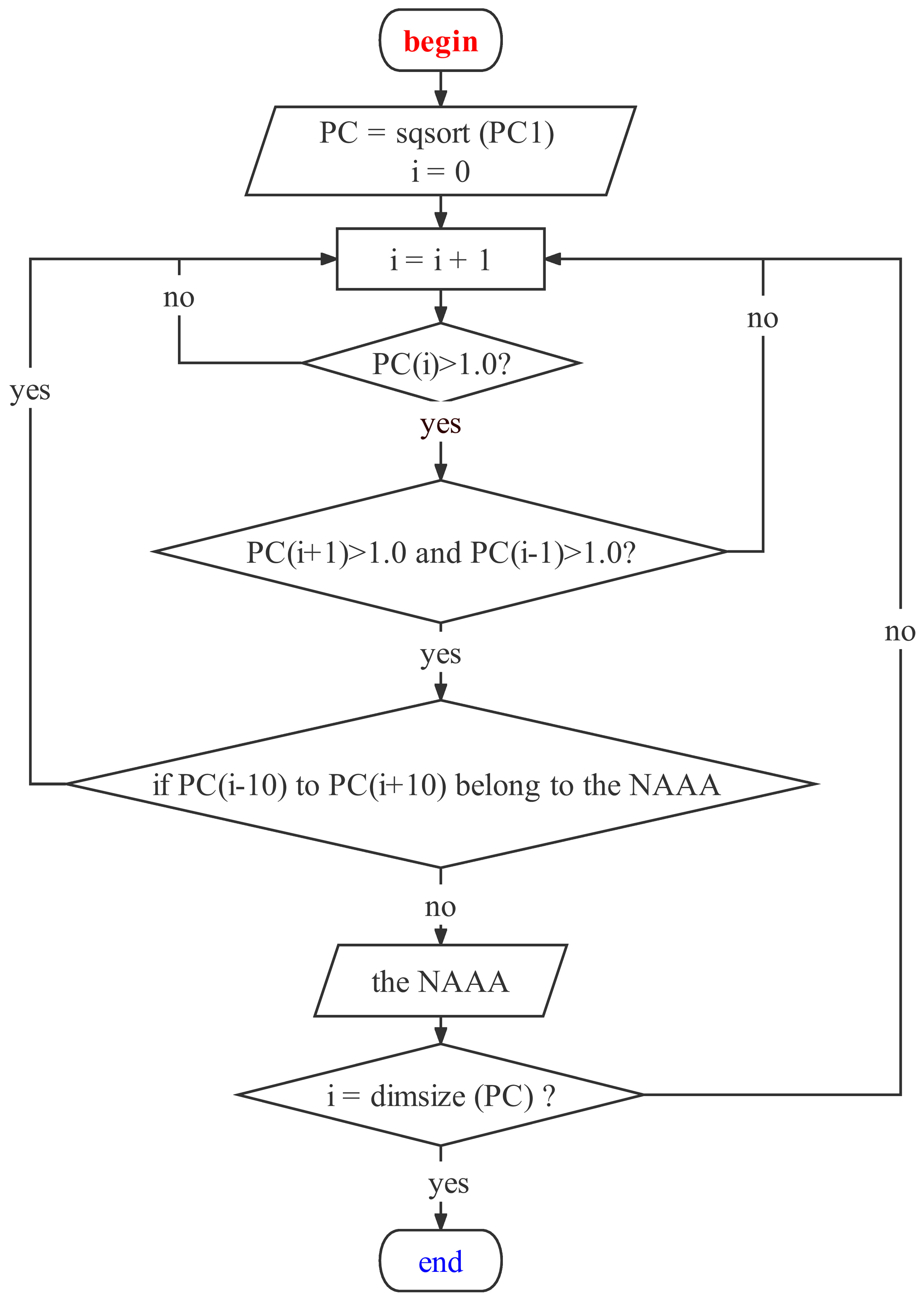
Figure 2 Process for selecting the NAAA events. Here, PC is the daily index of the NAAA, sqsort (PC) represents PC is sorted in descending order, dimsize (PC) is the size of one-dimensional array PC.

Second, the typical NAAA event is defined in the following way (Fig. 2). First, we rank the values of PC time series in descending order to select the date with the largest PC (i.e., the peak day). If the PC values on at least 3 d centered on the peak day all exceed one standard deviation, then this peak day is marked as day 0 of a strong NAAA event. Once a day 0 is found, no day within 21 d of the central date (day 0) can be defined as a strong NAAA event. This procedure prevents the algorithm from repeatedly counting the same strong NAAA event. Third, we repeat the above procedure until the values of PC do not exceed one standard deviation to guarantee that all the strong NAAA events are identified. Based on the above criteria (Fig. 2), 94 NAAA events in NDJ period 1979–2021 are selected in this study. This method is similar to that of Franzke et al. (2011), who studied the Pacific–North American teleconnection. In addition, the same method was used by Song et al. (2016), who studied the intraseasonal variation of the East Asian trough in winter.

In addition, to examine the propagation of anomalous Rossby waves generating the NAAA, we calculated the horizontal stationary wave activity flux (WAF), as defined by Takaya and Nakamura (2001). Daily reanalysis data; i.e., the zonal wind, meridional wind, and anomalous geopotential height, are used to calculate the vector W.

$$\begin{array}{}\text{(2)}& \mathit{W}={\displaystyle \frac{p\cos \mathit{\phi }}{\mathrm{2}\left|\mathbf{U}\right|}}\cdot \left(\begin{array}{l}\frac{U}{a^{\mathrm{2}}{\cos }^{\mathrm{2}}\mathit{\varphi }}\left[{\left(\frac{\partial {\mathit{\psi }}^{\prime }}{\partial \mathit{\lambda }}\right)}^{\mathrm{2}}-{\mathit{\psi }}^{\prime }\frac{{\partial }^{\mathrm{2}}{\mathit{\psi }}^{\prime }}{\partial {\mathit{\lambda }}^{\mathrm{2}}}\right]\\ +\frac{V}{a^{\mathrm{2}}\cos \mathit{\varphi }}\left[\frac{\partial {\mathit{\psi }}^{\prime }}{\partial \mathit{\lambda }}\frac{\partial {\mathit{\psi }}^{\prime }}{\partial \mathit{\varphi }}-{\mathit{\psi }}^{\prime }\frac{{\partial }^{\mathrm{2}}{\mathit{\psi }}^{\prime }}{\partial \mathit{\lambda }\partial \mathit{\varphi }}\right]\\ \frac{U}{a^{\mathrm{2}}\cos \mathit{\varphi }}\left[\frac{\partial {\mathit{\psi }}^{\prime }}{\partial \mathit{\lambda }}\frac{\partial {\mathit{\psi }}^{\prime }}{\partial \mathit{\varphi }}-{\mathit{\psi }}^{\prime }\frac{{\partial }^{\mathrm{2}}{\mathit{\psi }}^{\prime }}{\partial \mathit{\lambda }\partial \mathit{\varphi }}\right]\\ +\frac{V}{a^{\mathrm{2}}}\left[{\left(\frac{\partial {\mathit{\psi }}^{\prime }}{\partial \mathit{\varphi }}\right)}^{\mathrm{2}}-{\mathit{\psi }}^{\prime }\frac{{\partial }^{\mathrm{2}}{\mathit{\psi }}^{\prime }}{\partial {\mathit{\varphi }}^{\mathrm{2}}}\right]\end{array}\right),\end{array}$$

where W is the wave activity flux (unit: m² s⁻²), ψ ($=\mathrm{\Phi }/f$) is the geostrophic stream function, Φ (unit: m) is geopotential height, f (=2Ωsin ϕ) is the Coriolis parameter, p is the normalized pressure (pressure per 1000 hPa), and a is the earth's radius. λ and ϕ denote the longitude and latitude, respectively. U (=(UV)^T; unit: m s⁻¹) is the basic flow.

In addition to the methods mentioned above, composite analysis was also used to explore the atmospheric circulation patterns related to the NAAA that cause NDJ PM_2.5 pollution in the NCP. The zonal Fourier harmonic analysis of atmospheric circulation is also undertaken to obtain the parameters of the atmospheric waves (van Loon et al., 1973).

3 Results

3.1 Spatial and temporal characteristics of the northeast Asian anomalous anticyclone

Figure 3 presents the composite spatial distribution of atmospheric circulation for 94 NAAA events in NDJ period 1979–2021. The results show that there is a remarkably positive geopotential height anomaly at 500 hPa over northeast Asia with a strong center, i.e., about 40^∘ N, 135^∘ E (Fig. 3a). The NCP is located in the southwest of the NAAA, which is controlled by anomalous southeasterly winds related to the NAAA (Fig. 3c). This means that the East Asian winter monsoon in the NCP is weaker than normal (Wang et al., 2009), which is conduced to the accumulation of pollutants in the NCP (An et al., 2020). Additionally, the warmth and moisture flow from the West Pacific is advected by anomalous southeasterly wind into the NCP, favoring the hygroscopic growth of pollution (Ma et al., 2014). As a result, the NCP might experience heavy PM_2.5 pollution weather. Significantly, the maximum of the NAAA locates about 300 hPa with a vertical structure of westward tilt from 1000 to 850 hPa (Fig. 3b). The corresponding temperature anomaly is a dipole pattern at the lower (from 1000 to 300 hPa) and high (from 300 to 10 hPa) levels. That is to say that the lower level is a positive and the higher level a negative temperature anomaly (Fig. 3b), which might lead to a westward tilt structure of the NAAA via thermal wind and transient eddy feedback (Song et al., 2016).

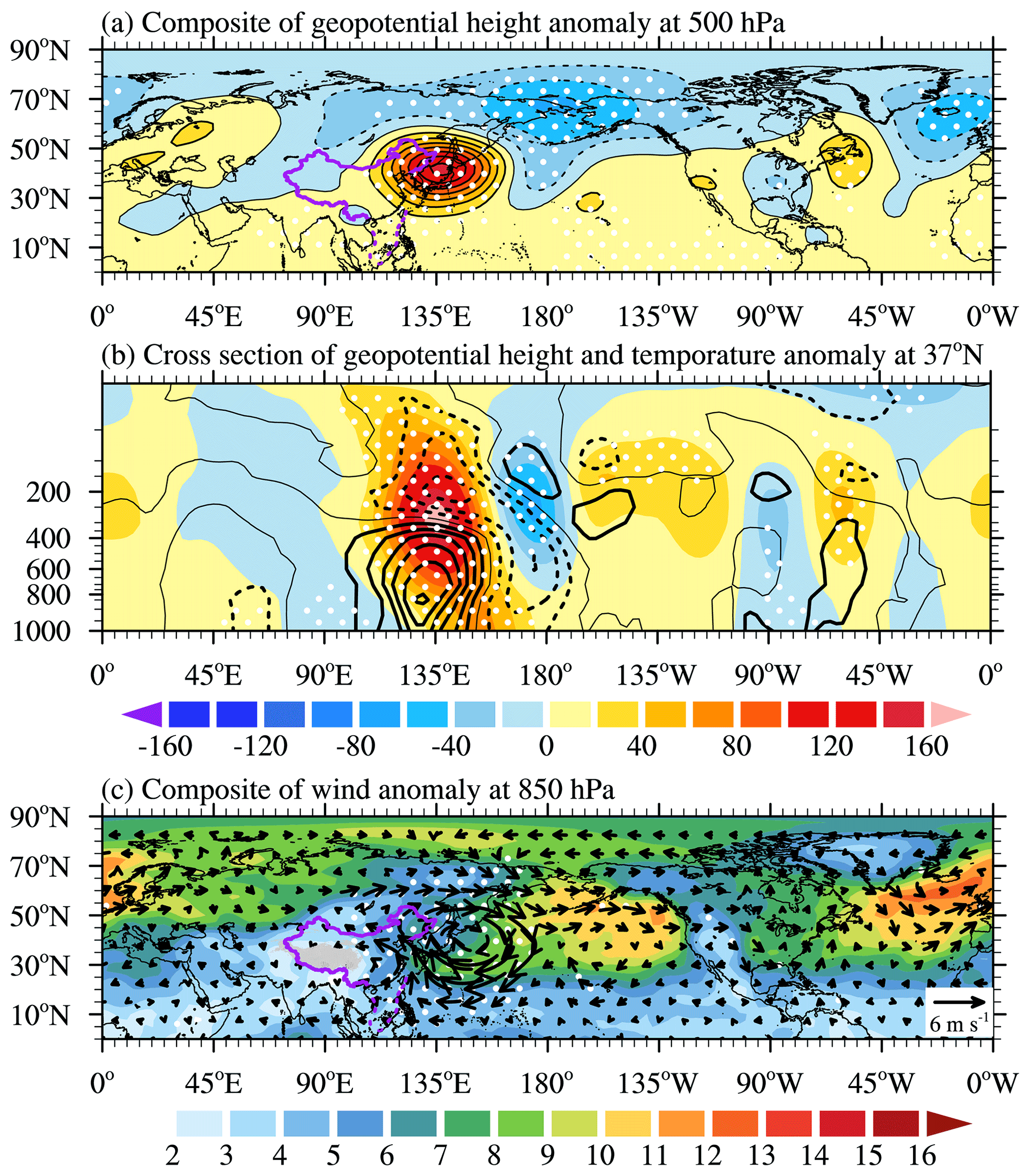
Figure 3 (a) Composite geopotential height anomaly (shading and contours; unit: m) at 500 hPa on the peak day of 94 NAAA events in NDJ period 1979–2021. (b) Composite longitude-height cross-section of geopotential height anomaly (shading; unit: m) and temperature anomaly (contours; unit: ^∘C) at 37^∘ N. (c) Composite wind vector (arrows; unit: m s⁻¹) and wind speed (shading; unit: m s⁻¹) at 850 hPa. The white dots denote the 99 % confidence level according to Student's t test.

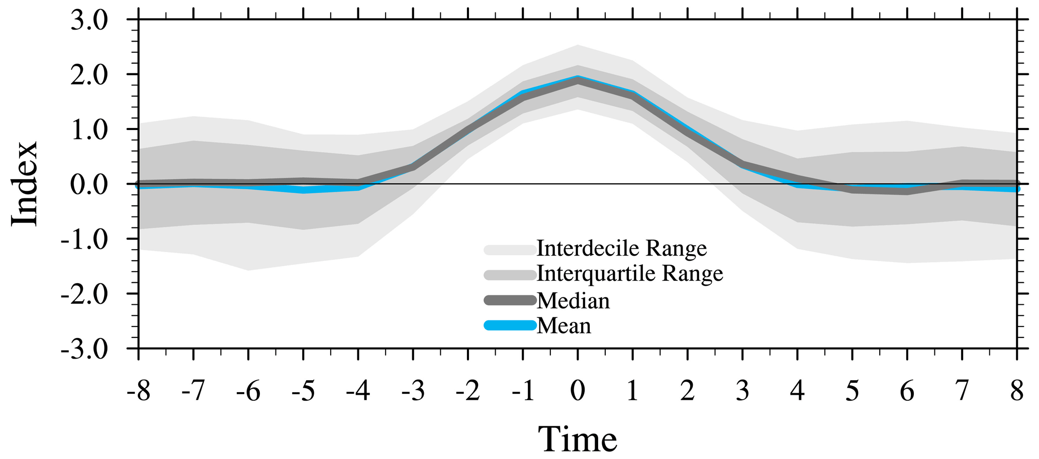
Figure 4 The temporal evolution of the standard PC time series for 94 NAAA events. In particular, black and blue curves represent mean and median value and light and deep gray fillings represent interdecile range and interquartile range, respectively.

To understand the duration of the NAAA, we show the temporal evolution of standardized daily PC time series of 94 NAAA events (Fig. 4). The PC values become positive from day −4, meaning that the NAAA starts to emerge. Note that the PC index reaches its maximum on day 0, and the PC index is almost zero or even negative after day 4, which implies the extinction of the NAAA with a life span of 8 d. Moreover, the 8 d life cycle of the NAAA suggests that it is enough to investigate the intraseasonal evolution and dynamics of the NAAA in the 21 d period described in the methods section. The question right now is where does the NAAA start?

To investigate the causes and evolution mechanism of the NAAA, the horizontal wave activity flux is calculated and shown in the form of arrows in Fig. 5. Distinctly, there is a positive geopotential anomaly over the Gulf Stream on day −8 and propagates eastward along the upper tropospheric polar front jet, which serves as a waveguide (Hoskins and Ambrizzi, 1993). On day −6 and the next 2 d, the Rossby wave energy reaches the region of northeast Asia, but there is no positive geopotential height anomaly there. Note that the significantly positive geopotential height anomaly appears in northeast Asia on days −3 and −2 (Fig. 5), which is an embryo of the NAAA, and means a rapid build-up of the NAAA. On day 0, the NAAA reaches the peak of its life cycle and wears out almost immediately on the next day (Figs. 4 and 5). There is almost no positive geopotential height anomaly in northeast Asia on day 4. On the interannual timescale, the NAAA seems to always occupy the whole winter and sustain a degradation effect on air quality in the NCP (Chang et al., 2016; An et al., 2020). On the synoptic scale, however, the life cycle of the NAAA is just 8 d. The results further suggest the necessity of studying the impact of the NAAA on PM_2.5 pollution in the NCP on the synoptic scale.

Figure 5 Composite evolution of geopotential height anomaly (shading; unit: m) and the WAF (arrows; unit: m² s²) at 500 hPa on days −8, −6, −4, −2, 0, +2, +4, +6 and +8 in 94 NAAA events since 1979. The white dots denote the 99 % confidence level according to Student's t test.

For a deeper understanding of the generation of the NAAA with a westward tilting structure from wave theory, zonal harmonic analysis is used in this investigation. Wavenumbers 1–10 are the spectral components on wavenumber domains produced by Fourier transform in the spatial domain. Among them, wavenumbers 1–2 represent ultralong waves, wavenumbers 3–5 denote long waves, and wavenumbers 6–10 are synoptic waves. Figure 6 compares the height–longitude cross-section of zonal harmonic wave anomalies on the peak day of the NAAA, overlapped with raw geopotential height anomaly. Note that the reason why other wavenumbers (i.e., wavenumbers 5–10) are not shown in Fig. 6 is that their shapes are quite different from the shape of the NAAA. From Fig. 6, we find that the shapes of wavenumbers 3–4 (referred as the quasi-stationary wave) is consistent with that of the NAAA in general. The results suggest that wavenumbers 3–4 might play an important role in the generation and elimination of the NAAA (Fig. 6). The amplitudes and variances of the harmonics also support the significant roles played by the Rossby wave (Fig. 7). For instance, the amplitudes and variances of wavenumbers 3–4 are significantly greater than other wavenumbers (Fig. 7). In addition to the quasi-stationary wave characterized by wavenumbers 3–4, transient eddy feedback (2–8 d on the timescale) due to a baroclinic atmosphere also plays an important role in the development of the NAAA (i.e., contributes to rapid build-up of the NAAA) (Song et al., 2016).

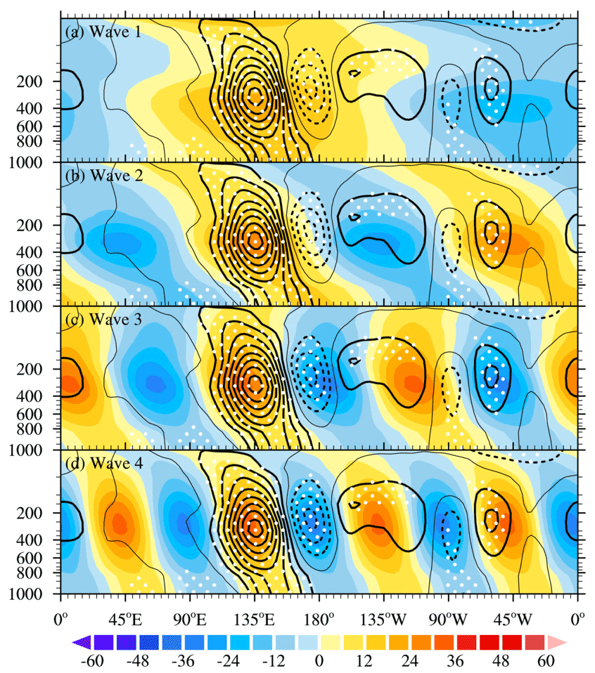
Figure 6 Cross-section of zonal harmonic analysis of geopotential height anomaly. (a) Wavenumber 1, (b) wavenumber 2, (c) wavenumber 3 and (d) wavenumber 4 (shading; unit: m) and geopotential height anomaly (contours; unit: m) from 1000 to 10 hPa on peak day of 94 NAAA events. The white dots denote the 99 % confidence level according to Student's t test.

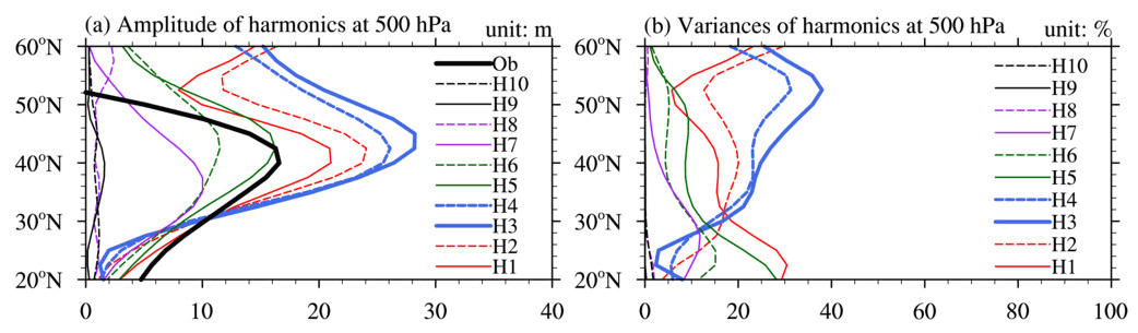
Figure 7 Zonal harmonic analysis of geopotential height anomaly at 500 hPa on the peak day of 94 NAAA events since 1979. (a) Amplitude harmonics of waves 1–10, (b) variances harmonics of wavenumbers 1–10. In particular, the thick black curve (Ob) represents zonal mean geopotential height anomaly in the peak day of 94 NAAA events.

3.2 The northeast Asian anomalous anticyclone in relation to variation of PM_2.5 pollution in the NCP

Section 3.1 investigates the spatiotemporal characteristics and evolution mechanism of the NAAA on the intraseasonal timescale, how it relates to air quality in the NCP, and what potential conditions give rise to this regime. Figure 8 presents composite PM_2.5 concentration anomaly from days −4 to 4 of 51 NAAA events in NDJ period 2000–2021. The PM_2.5 concentration tends to increase on day −3 and then increases rapidly after day −2. By 1 d before the peak of the NAAA, the PM_2.5 concentration anomaly reaches a maximum and maintains it on the next day. On day 2 after the peak of the NAAA, the positive PM_2.5 concentration anomaly tends to dissipate. Generally, under the background of the NAAA, the NCP experiences heavy PM_2.5 pollution for 4 d. Similarly, we investigate the evolution of PM_2.5 pollution in the NCP based on the TAP PM_2.5 concentration and observed PM_2.5 concentration data since 2013 (not shown). The results are in line with the above conclusions drawn using TAP PM_2.5 concentration data since 2000, suggesting our findings are reliable despite PM_2.5 concentration data from machine learning by Geng et al. (2021a).

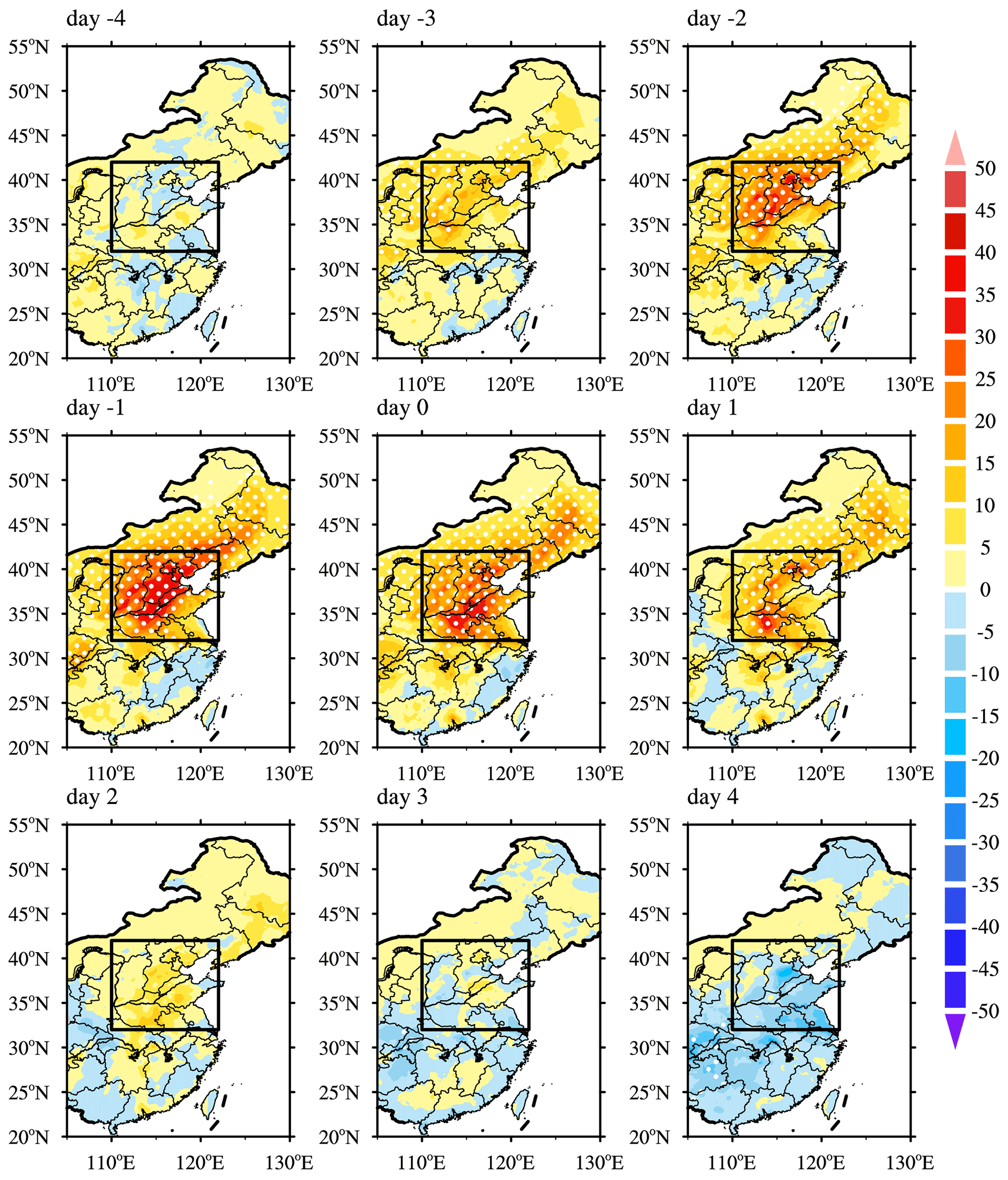
Figure 8 Composite evolution of PM_2.5 concentration anomaly (shading; unit: µg m⁻³) from day −8 to day 8 in 51 NAAA events in NDJ period 2000–2021. The white dots denote the 99 % confidence level according to Student's t test.

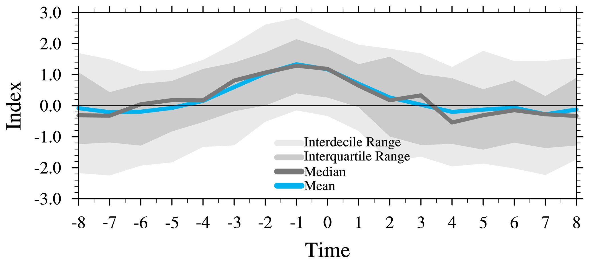
Figure 9 The same as Fig. 4 except for PM_2.5 concentration anomaly in 51 NAAA events in NDJ period 2000–2021.

Figure 9 shows daily PM_2.5 concentration anomaly averaged in the NCP for 8 d before and after the peak day of the NAAA. The results indicate a distinct evolution of PM_2.5 pollution compared with that of the NAAA. Clearly, PM_2.5 concentration begins to increase after day −4 with a peak on day −1 and then decreases gradually to zero on day 2. The NCP has gone through significant PM_2.5 pollution for days −2 to 1 of the peak day of the NAAA (Fig. 9), which is consistent with the conclusions from Fig. 8. Significantly, the interquartile range (specially interdecile range) of area-averaged PM_2.5 concentration anomaly during days −2 to 1 has parts less than 0, meaning that not all of the NAAA events can cause PM_2.5 pollution for at least 3 d (i.e., days −2 to 0) in the NCP. This makes us aware that the probability of PM_2.5 pollution events in the NCP related to the NAAA should be further examined.

Table 1 The probability of the NAAA in relation to PM_2.5 pollution in the NCP.

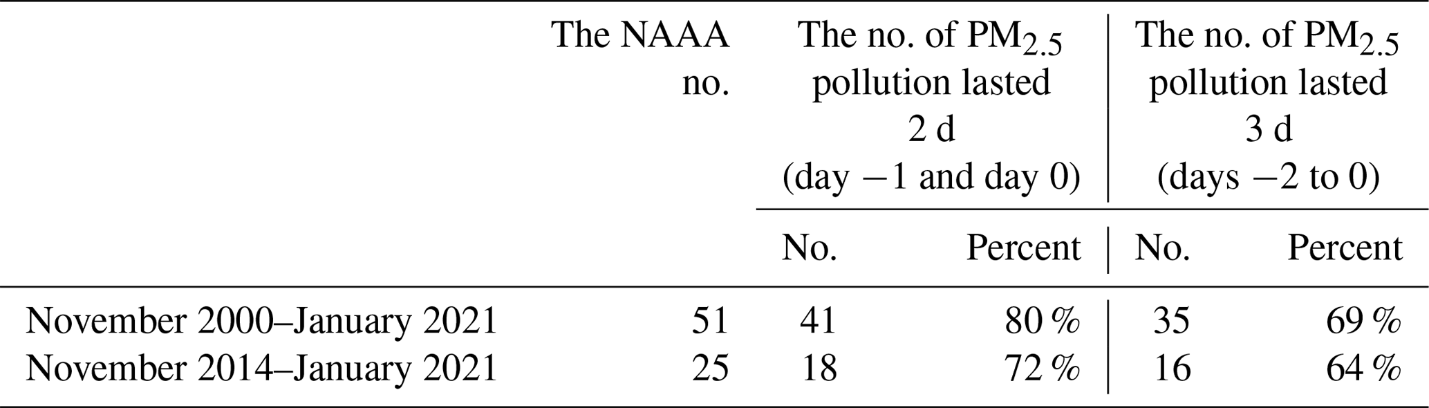
The probability of PM_2.5 pollution under the background of the NAAA is presented in Table 1, and the event of PM_2.5 pollution is defined here as exceeding 0 for at least 3 d (i.e., days −2 to 0) for region-averaged PM_2.5 concentration anomaly in the NCP (Table 1). The probability of the NAAA in relation to PM_2.5 pollution for at least 3 d in the NCP is 69 % if we start counting from 2000. This is 64 % when we start counting from 2014. Additionally, the probability of the NAAA in relation to PM_2.5 pollution for at least 2 d in the NCP is higher (i.e., 80 % and 72 %) than at least 3 d. These results further illustrate that meteorological factors, especially the NAAA, play a crucial role in NDJ PM_2.5 concentration in the NCP in spite of a decline of 42 % of the annual mean PM_2.5 concentrations between 2013 and 2018 in China (Nature Geoscience, 2019), which is in line with results by Dang and Liao (2019). From what is mentioned above, we come to the robust conclusion that 69 % of the NAAA might cause NDJ PM_2.5 pollution for at least 3 d in the NCP during the period of 2000–2021.

3.3 Why does PM_2.5 pollution occur in the NCP before the peak day of the NAAA

From the previous section, we see that PM_2.5 pollution in the NCP begins to deteriorate significantly from day −2 of the peak day of the NAAA. What sort of meteorological conditions causes this observed fact of PM_2.5 pollution? The NAAA is usually accompanied by southerly wind anomalies on its western flank, corresponding to lower ABLH and weaker surface winds (Yin et al., 2017). We therefore explore the possible meteorological conditions favouring PM_2.5 pollution in terms of dynamics (i.e., diffusion condition) and thermodynamics (i.e., stability). In Fig. 10, the evolution of the ABLH anomaly 4 d before and after the peak day of the NAAA is shown. The results show that there is remarkably negative ABLH anomaly on day −3, which means a shallow atmospheric boundary layer, favorable to accumulation of pollutants. It should be noted that the ABLH reduction 1 d prior to the appearance of PM_2.5 pollution, which provides sufficient time for the accumulation of pollutants so that the occurrence of PM_2.5 pollution on the following day (Figs. 8 and 11). On day 1, the negative ABLH anomaly decreases abruptly, corresponding PM_2.5 pollution is also slightly lowered (Figs. 8 and 11). On the next day (i.e., day 2), there is no significantly negative ABLH anomaly and the corresponding PM_2.5 pollution also almost disappears in the NCP (Figs. 8 and 11).

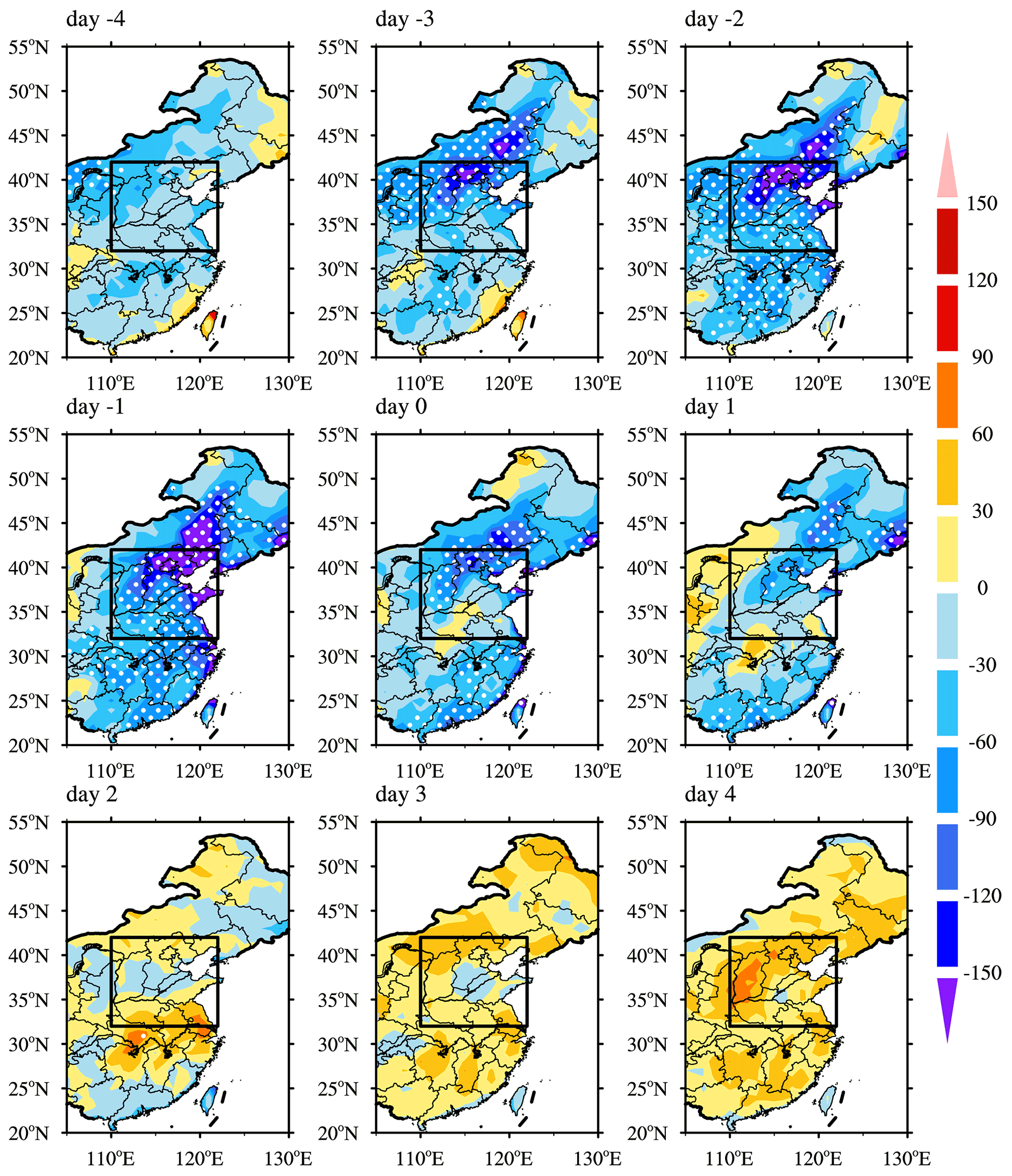
Figure 10 The same as Fig. 8 except for the ABLH anomaly (shading; unit: m).

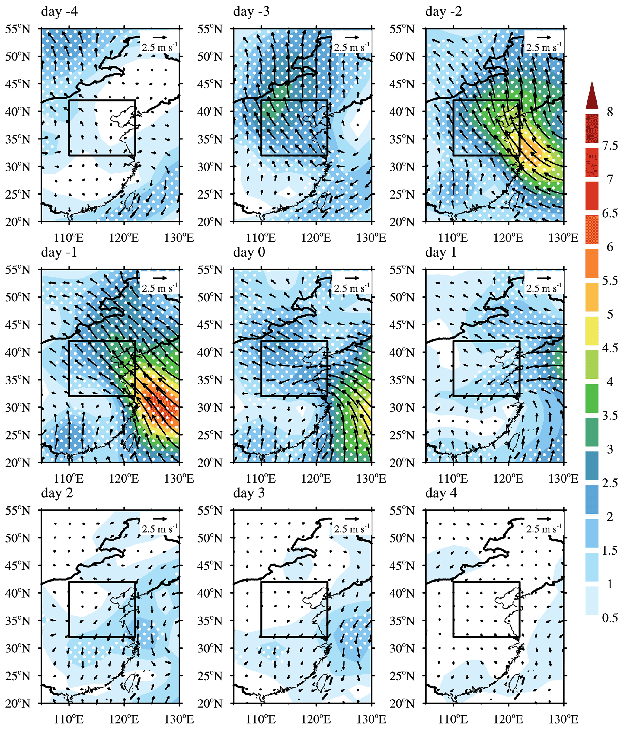
Figure 11 The same as Fig. 8 except for anomalous wind vector (arrows; unit: m s⁻¹) and anomalous wind speed (shading; unit: m s⁻¹) at 1000 hPa.

Similar conclusions can be drawn from the wind field for 4 d before and after the peak day of the NAAA, which represents a diffusion condition for PM_2.5 pollution (e.g., Yang et al., 2016; Liu et al., 2017). As shown in Fig. 11, the NCP is mainly controlled by anomalous southerly winds with a negative divergence anomaly (not shown), which also appears 1 d (i.e., day −3) earlier than heavy PM_2.5 pollution in the NCP. The intensity and range of southerly winds increase significantly on the following 2 d (i.e., day −1 and day 0). The intensity and range of southerly winds, however, shrink rapidly on day 1 and almost disappear on day 2. This process is consistent with PM_2.5 pollution in the NCP except that the establishment of favorable wind field is earlier (by 1 d) than the occurrence of PM_2.5 pollution. The earlier emergence of southerly wind anomaly with a negative divergence anomaly and shallow atmospheric boundary layer together facilitate the accumulation of pollutants, leading to the occurrence of PM_2.5 pollution the following day. The maintenance of these two parameters leads to PM_2.5 pollution lasting for the next 2 d. While the later weakening and even disappearance of southerly wind anomaly and shallow atmospheric boundary layer improve PM_2.5 quality in the NCP after the day 1 of peak day of the NAAA.

Overall, both the dynamic and thermodynamic conditions associated with the NAAA result in heavy PM_2.5 pollution in the NCP. Most importantly, PM_2.5 pollution in the NCP happens 1 d earlier than the peak of the NAAA, which provides a reference for prediction of PM_2.5 pollution in the NCP on the synoptic scale. In addition, if we take the positive geopotential height anomaly over domain 45–60^∘ N, 80–100^∘ E as a predictor, the potential prediction of PM_2.5 pollution in the NCP might be extended to 5 d (Fig. 5). Now what we wonder is why the favorable meteorological conditions related to the NAAA appear before the peak day of the NAAA?

To further understand the physical mechanisms of the NAAA favoring occurrence of PM_2.5 pollution in the NCP, the vertical structure of temperature and geopotential anomaly and their evolution in a position of 37^∘ N, 115^∘ E are shown in this section. As shown in Fig. 12, temperature anomaly features a backward tilt with height below 700 hPa, meaning that the higher temperature anomaly moves from a higher to a lower level from days −3 to −1, which is easier to cause a potential thermal inversion. In addition, the ABLH anomaly is significantly negative in this period (Figs. 10 and 12), corresponding to the negative PM_2.5 concentration anomaly in the NCP (Fig. 8). Above 700 hPa it features a forward tilt with height implying that the positive temperature anomaly moves from a lower to a higher level from days −1 to 2, which is unfavorable for the formation of a potential thermal inversion. In addition, there is significantly anomalous ascending motion in the troposphere on days −3 to −1 (not shown), which might suppress intrusion of clean air from the upper levels (i.e., above 300 hPa) to the lower levels, resulting in a shallower atmospheric boundary layer (Zhong et al., 2019). However, the negative ABLH anomaly decreases rapidly from days −1 to 2, and the corresponding air quality in the NCP is gradually improved (Figs. 10 and 12). The characteristics based on area-averaged temperature and ABLH anomaly in the NCP are similar to the results based on a single position (not shown).

Figure 12 Composite time-height cross-section of temperature anomaly (shading; unit: m) at 37^∘ N, 115^∘ E from the developing stage (day −8 to day 0) to the decay stage (day 0 to day +8) for 51 NAAA events in NDJ period 2000–2021. The white dots denote the 99 % confidence level according to Student's t test. Black bar charts represent the variation of the ABLH anomaly (bars; unit: m) at 37^∘ N, 115^∘ E from the developing stage (day −8 to day 0) to the decaying stage (day 0 to day +8) of 51 NAAA events in NDJ period 2000–2021. Especially, the coordinates on the right represent the value of the ABLH anomaly. The horizontal line denotes zero of the ABLH anomaly.

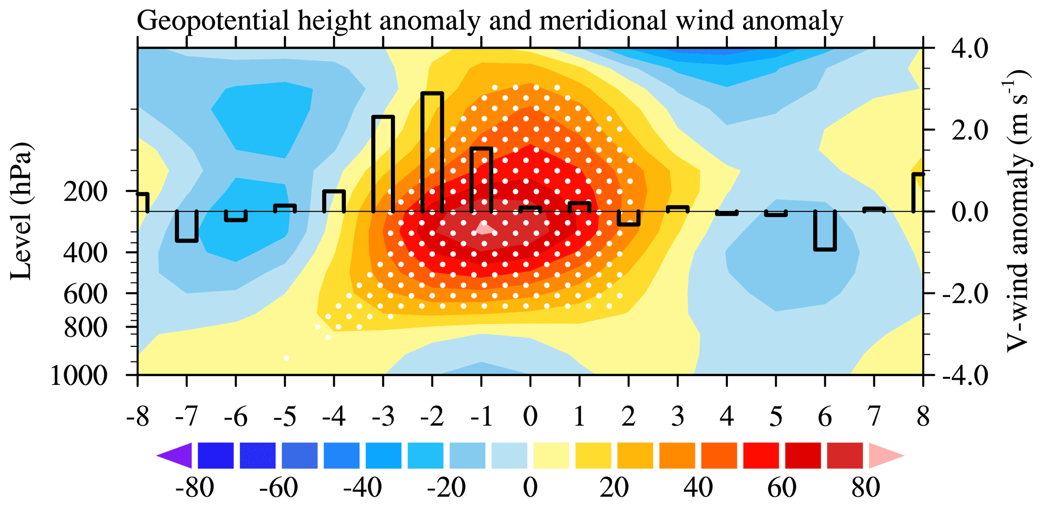
Figure 13 The same as Fig. 12, but for geopotential height anomaly (shading; unit: m) and 1000 hPa meridional wind anomaly (bars; unit: m s⁻¹). Positive values of meridional wind anomaly represent southerly wind anomaly.

Similarly, we checked the evolution of geopotential height anomaly and meridional wind anomaly with time and height in point (37^∘ N, 115^∘ E). Not surprisingly, positive geopotential height anomaly shows a sudden enhancement in the whole troposphere from days −4 to 3 (Fig. 13), which is in line with the result in Fig. 4b. This means a rapid build-up of the NAAA with a sudden enhancement of anomalous southerly winds. As is well-known, PM_2.5 pollution is closely tied to lower wind field, especially surface wind field (e.g., Yang et al., 2016; Liu et al., 2017; Yin et al., 2017). Therefore, on day −3, the NAAA rapidly builds up with the sudden increase of geopotential height anomaly and southerly wind anomaly (Figs. 7 and 13), resulting in PM_2.5 pollution prior to the peak day of the NAAA. We can draw the same conclusion compared with an area-averaged geopotential height anomaly and 1000 hPa meridional wind anomaly in the NCP.

4 Conclusions and discussion

In this study, we investigated the characteristics and evolution mechanisms of the NAAA on the intraseasonal timescale and the associated PM_2.5 pollution in the NCP in NDJ. In particular, the intraseasonal NAAA has a life span of about 8 d with a structure of westward tilt with height, and its evolution is closely tied to the Rossby wave from upstream (i.e., the North Atlantic). On day −8, there is significant circulation anomaly over the Gulf Stream and downstream propagation in the form of the Rossby wave. The NAAA reaches its peak on day 0 and decreases rapidly the next day. According to harmonic analysis, the NAAA with a westward tilt may be related to the wavenumbers 3–4. Additionally, the NAAA is also enhanced by the transient eddy, which can be induced by a weak baroclinic atmosphere with the characteristic of vertical dipole pattern of temperature. For instance, Song et al. (2016) found that the transient eddy feedback leads to 30 % of the NAAA amplification using the geopotential height tendency equation.

Further results show that 69 % of the NAAA in NDJ period of 2000–2021 causes regional PM_2.5 pollution for at least 3 d (80 % for at least 2 d) in the NCP and its peak day lags behind the occurrence of PM_2.5 pollution for 2 d. The composite analysis reveals that the shallower atmospheric boundary layer and stronger surface southerly wind anomaly (weaker northerly wind) associated with the NAAA in the NCP appear 1 d prior to PM_2.5 pollution, which provides dynamic and thermal conditions for the accumulation of pollutants and finally occurrence of PM_2.5 pollution on the following day. We also find that the stagnant air and weak ventilation conditions are determined by a special vertical distribution of temperature anomaly and a rapid build-up of the NAAA.

It is well known that the wet deposition through scavenging by rainfall is an effective way to remove atmospheric aerosols and soluble gases (e.g., Atlas and Giam, 1988). When the NAAA appears, southern China tends to experience heavy rainfall and vice versa in the NCP (not shown) (e.g., Ma et al., 2018; An et al., 2020, 2022), which is not only conducive to the wet removal of aerosol in the NCP but usually deteriorates air quality in the NCP via a local north-south circulation (not shown) (An et al., 2020, 2022; Mei et al., 2021).

In addition, as shown in Figs. 8–9, PM_2.5 pollution occurred over the NCP 1 d before the peak day of the NAAA, which implies the former might exert an impact on its formation and thus form a positive feedback of PM_2.5 pollution-atmospheric circulation. The increases in aerosols, especially absorbing aerosols, have been reported to heat the air, and therefore lead to atmospheric stagnation (e.g., Ding et al., 2016) and weaker ventilation over the NCP (e.g., Lou et al., 2019). Therefore, the PM_2.5 accumulation before the peak day of the NAAA may also cause or at least intensify the dynamical or thermodynamical anomalies, which in turn might support the formation of PM_2.5 pollution over the NCP. This is a potentially interesting topic that deserves further investigation in the future.

In brief, the NAAA and associated meteorological parameters play a crucial role in formation of NDJ PM_2.5 pollution in the NCP on the intraseasonal timescale, which is slightly different from its role in wintertime PM_2.5 pollution in this region on the interannual timescale. For example, we cannot draw a conclusion that the peak time of the NAAA lags behind PM_2.5 pollution in the NCP in NDJ on the interannual timescale. In addition, there is usually an anomalous descending motion in the NCP in NDJ on the interannual timescale (An et al., 2020), while on the intraseasonal timescale there is an anomalous ascending motion in this region (not shown). The shortcoming of this study is that it only investigated the influence of the NAAA on PM_2.5 pollution in the NCP in NDJ on the intraseasonal timescale. It should be noticed that cyclone anomaly in northeast Asia, as a pattern of out of phase of the NAAA (Wang et al., 2009; Song et al., 2016), might be a favorable atmospheric circulation to improve PM_2.5 quality, which should also be studied in future.