Long- and short-term temporal variability in cloud condensation nuclei spectra over a wide supersaturation range in the Southern Great Plains site

When aerosol particles seed the formation of liquid water droplets in the atmosphere, they are called cloud condensation nuclei (CCN). Different aerosols will act as CCN under different degrees of water supersaturation (relative humidity above 100 %), depending on their size and composition. In this work, we build and analyze a best-estimate CCN spectrum product, tabulated at ∼ 45 min resolution, generated using high quality data from seven independent instruments at the U.S. Department of Energy Atmospheric Radiation Measurement (ARM) Southern Great Plains site. The data product spans a large supersaturation range, from 0.0001 % to ∼ 30 %, and time period of 5 years, from 2009–2013, and is available on the ARM data archive. We leverage this added statistical power to examine relationships that are unclear in smaller datasets. Our analysis is performed in three main areas. First, probability distributions of many aerosol and CCN metrics are found to exhibit skewed log-normal distribution shapes. Second, clustering analyses of CCN spectra reveal that the primary drivers of CCN differences are aerosol number size distributions, rather than hygroscopicity or composition, especially at supersaturations above 0.2 %, while also allowing for a simplified understanding of seasonal and diurnal variations in CCN behavior. The predictive ability of using limited hygroscopicity data with accurate number size distributions to estimate CCN spectra is investigated, and the uncertainties of this approach are estimated. Third, the dynamics of CCN spectral clusters and concentrations are examined with cross-correlation and autocorrelation analyses. We find that CCN concentrations change rapidly on the timescale of 1–3 h, with some conservation beyond that which is greatest for the lower supersaturation region of the spectrum.

1 Introduction

The interactions between atmospheric aerosol particles and ambient water vapor are key drivers of the formation of haze and clouds. Particles are the nuclei upon which liquid water first condenses to form haze and cloud droplets, thereby affecting visibility, cloud microphysical properties, and precipitation. Water uptake by particles depends upon their size and chemical composition, as well as on ambient environmental conditions, and on their rates of change. Particles that are identified as cloud condensation nuclei (CCN) are typically those that are predicted to form cloud drops at water supersaturations (SS_w) of 1 % or lower, which are conditions believed to be typical of most clouds that are formed in weak to moderate updrafts. Based on average aerosol characteristics, and typical atmospheric aerosol number size distributions (shortened to size distributions hereafter), the number concentrations of particles active as CCN are thus generally assumed to correspond to those particles in the 80–300 nm dry diameter size range. Instruments designed to directly measure the number concentrations of activated particles at fixed SS_w are also typically limited to 2 % SS_w as an upper bound on the measurement range (Uin, 2016).

However, supersaturations and particle sizes outside of these ranges are also of atmospheric interest. In deep convection with intense updrafts, and in regions of very low existing particle or droplet surface area concentrations, SS_w can build rapidly to high levels, as the condensation sink rates are so low relative to the rate of supersaturation generation (Pinsky et al., 2012). Those high SS_w conditions may be sufficient to allow particles smaller than 40 nm to serve as cloud condensation nuclei. Thus, despite their relatively short lifetimes in the atmosphere compared with larger accumulation mode particles, high concentrations of small particles can potentially influence cloud microphysical processes leading to precipitation formation or evaporation. It is now recognized that the nucleation of new particles from the gas phase, generating particles on the order of 10 nm in diameter which subsequently grow, occurs in many regions of the troposphere and is an important control on global atmospheric aerosol number concentrations (Hodshire et al., 2016; Bianchi et al., 2016; Venzac et al., 2008; Pierce et al., 2014; Nieminen et al., 2018).

At the other end of atmospherically relevant supersaturations, droplet formation may occur at very low SS_w, where CCN concentrations are very difficult to probe. For example, the slow cooling rates in radiation fogs allow vapor scavenging to effectively compete with the generation of supersaturation, and thus, maximum SS_w conditions reached in fogs can be below 0.05 % (Gerber, 1991; Low, 1975; Shen et al., 2018), suggesting that only larger and more hygroscopic particles can participate in fog droplet formation. The cloud physics community has had a long-standing interest in elucidating the microphysical roles of giant CCN (GCCN), that is, relatively large particles that activate at very low SS_w, with ∼ 0.01 % or less. Specifically, GCCN are hypothesized to control the initiation of drizzle and precipitation in shallow clouds (Cohard et al., 1998; Johnson, 1982; Feingold et al., 1999; Cheng et al., 2009; Hudson et al., 2011; Posselt and Lohmann, 2008; Levin and Cotton, 2009; Gantt et al., 2014; Jung et al., 2015).

Their potentially controlling roles in fog, cloud, and precipitation formation have motivated interest in direct measurements of the number concentrations of CCN active over a range of atmospherically relevant SS_w, with modern instrumentation making long-term, unattended monitoring possible. Here, we analyze observations of CCN spectra from the United States Department of Energy's Atmospheric Radiation Measurement's (ARM) Southern Great Plains (SGP) site located in north central Oklahoma for the 5-year period from 2009–2013. The CCN measurement instrumentation deployed at this site is typically limited to stable operation over the 0.1 % to 1 % SS_w range. As described further below, we extend those observations to a broader supersaturation range of interest using ancillary aerosol observations, described briefly in Table 1, creating a CCN estimate relevant for clouds ranging from fog through to intense deep convective updrafts. These observations are especially important for modeling studies of aerosol impacts on clouds in this region that use CCN number concentrations as a basis for determining their aerosol initial conditions (Saleeby et al., 2016; Marinescu et al., 2017; Glenn et al., 2020). This extensive CCN dataset is subsequently analyzed using methods to leverage its range and statistical power to characterize and understand the statistical distributions, seasonal and diurnal variations, and dynamics of CCN spectra at this site.

2 Methods

This work builds upon prior work reported in Marinescu et al. (2019). In that study, for the same 2009–2013 time period studied herein, aerosol data from three instruments deployed at the SGP site were averaged over ∼ 45 min intervals and merged into dry aerosol size distributions, n(D_p), spanning a 7 nm < particle dry diameter, D_p < 14 µm. We build upon that work by combining those merged size distributions with information on aerosol hygroscopicity, κ (Petters and Kreidenweis, 2007), taken over the same ∼ 45 min intervals. The κ values were obtained via measurements of diameter growth factors (GFs) at 90 % relative humidity measured by a humidified tandem differential mobility analyzer (HTDMA; Collins, 2010b; Mahish and Collins, 2017). The procedure for integrating these data into a CCN spectrum is described more fully in Appendix A but is reviewed briefly here. All base instrument measurements used in the data construction are shown in Table 1, along with a brief description of their associated measurement and the aerosol size range probed.

Table 1 Base measurements used in the dataset construction.

^* The upper size cut will depend on instrument inlet losses.

The critical saturation ratio, S_c, at which a particle with dry particle diameter D_p can be activated into a cloud drop is determined by finding the maximum of the following equation (Petters and Kreidenweis, 2007):

$$\begin{array}{}\text{(1)}& {\displaystyle }S\left(D\right)={\displaystyle \frac{D^{\mathrm{3}}-D_{\mathrm{p}}^{\mathrm{3}}}{D^{\mathrm{3}}-D_{\mathrm{p}}^{\mathrm{3}}(\mathrm{1}-\mathit{\kappa })}}\exp \left({\displaystyle \frac{A}{D}}\right)\text{(2)}& {\displaystyle }A={\displaystyle \frac{\mathrm{4}{\mathit{\sigma }}_{\mathrm{s}/\mathrm{a}}{M}_{\mathrm{w}}}{RT{\mathit{\rho }}_{\mathrm{w}}}},\end{array}$$

where D is the droplet diameter, ρ_w is the density of water, M_w is the molecular weight of water, ${\mathit{\sigma }}_{\mathrm{s}/\mathrm{a}}$ is the surface tension of the solution/air interface, R is the universal gas constant, and T is temperature. Saturation ratio, S, and water supersaturation percent, SS_w are related by the following:

$$\begin{array}{}\text{(3)}& {\mathrm{SS}}_{\mathrm{w}}=\left(S-\mathrm{1}\right)\cdot \mathrm{100}.\end{array}$$

The functional relationship between D_p, κ, and S_c can be more readily illustrated by the approximate relationship that is valid for κ > 0.2 (Petters and Kreidenweis, 2007), where SS_w,c is the critical water supersaturation percent, as follows:

$$\begin{array}{}\text{(4)}& {\displaystyle \frac{{\mathrm{SS}}_{\mathrm{w},\mathrm{c}}}{\mathrm{100}}}\cong {\left\{{\displaystyle \frac{\mathrm{4}{A}^{\mathrm{3}}}{\mathrm{27}{D}_{\mathrm{p}}^{\mathrm{3}}\mathit{\kappa }}}\right\}}^{\mathrm{1}/\mathrm{2}}.\end{array}$$

From Eq. (4) it can be seen that information on the aerosol size distribution, n(D_p), and the variation of κ with dry diameter, can be used to compute the critical SS_w corresponding to each selected dry size used in Eq. (4). It should be noted that the approximation in Eq. (4) is only used for demonstration here, with the full methods described in Appendix A. In practice, the size distribution is discretized to obtain the total number concentrations in each selected dry diameter bin, i.e., 222 logarithmically spaced bins in this work, and a constant κ is assumed across each selected bin. To produce the size-dependent κ distribution, measurements of aerosol hygroscopic growth were made for seven different sizes (Fig. A2), which were subsequently processed to obtain a single weighted κ value for each size. In this study, these κ values are then interpolated linearly between measured values, with invariant κ beyond the largest and smallest sizes (below ∼ 10 nm and above ∼ 600 nm). The cumulative spectrum of CCN concentration, CCN(SS_w), can then be constructed, which defines the total number of particles that can be activated at a particular SS_w. Figure 1a shows an example of the measured n(D_p) and κ (D_p), and the resulting CCN spectrum is shown in Fig. 1b.

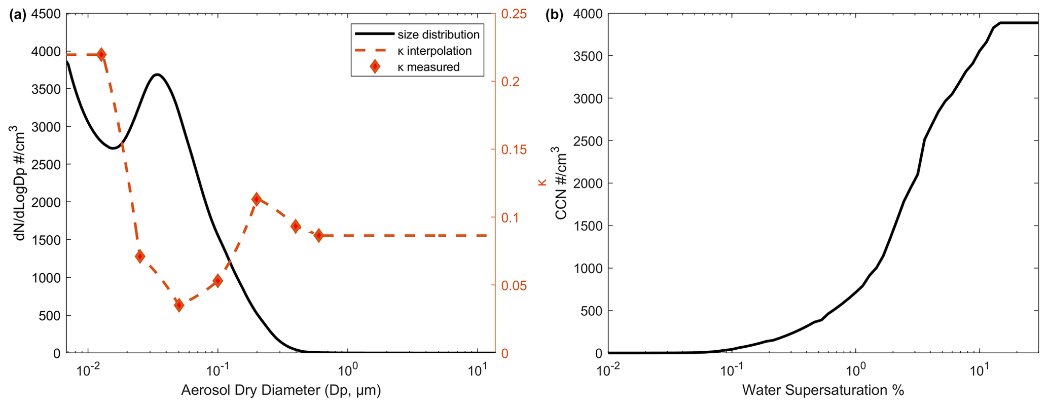
Figure 1 Example data products from 30 January 2012 at 5:20 UTC, with the size (left; black solid line), κ (left; orange dashed line), and CCN (right) distributions shown. Measured κ points are shown with markers, with linearly interpolated values as dashed lines.

Available data from the measurement suite include direct, concurrent, and co-located observations of cumulative CCN number concentrations at selected supersaturations, which were used to check the accuracy of the initial CCN spectra, reconstructed from size distributions and hygroscopicity measurements discussed above that are between 0.1 % and 1 % supersaturation, and adjusted as needed. There were two additional instruments that provided separate, independent, and continuous observations and that were used to constrain the reconstructed spectra, namely a nephelometer that measured total particle scattering coefficients and an aerosol chemical speciation monitor (ACSM) that measured nonrefractory, speciated submicron mass concentrations. Both of these observations emphasize the larger particle sizes (generally > 300 nm) and thus served as constraints on the particles contributing strongly at the lowest supersaturations, for which no direct observations exist. At the other end of the size distribution, the smallest particles are expected to require the highest supersaturations for activation, but neither the size distribution nor κ are well constrained observationally. Reasonable assumptions are applied to extrapolate the CCN spectrum beyond SS_w=1 %, which is the approximate upper limit of the CCN counter. In total, data from five instruments are merged and then constrained with observations from two additional instruments to produce a best-estimate CCN spectrum for each ∼ 45 min interval, as described more fully in Appendix A. Resulting size distributions range from 0.0068 to 13.8 µm (bin centers), with corresponding CCN spectra generated for SS_w from 0.0001 % to ∼ 30 % SS_w (100.0001 to 130 % RH). The SS_w range is chosen to span the entire range of particle activations. The largest and most hygroscopic measured particles activate at 0.0001 % SS_w, while the smallest and least hygroscopic at ∼ 30 % SS_w. As noted in the data availability statement below, the final merged data are available in the Department of Energy's (DOE) ARM archive. This dataset is subsequently analyzed using several different methods. The results of these analyses are discussed in Sect. 3 below, while the details of analytical methods are found in Appendix B, for the skewed log-normal fitting procedures, Appendix C, for the clustering analysis, and Appendix D, for the non-periodic autocorrelation and fits.

3 Results and discussion

3.1 Distribution characteristics

While we expect the final merged data over the entire range to be useful, all observations are not equally reliable for several reasons. In the size distributions, the lowest size bins are generated using a fitting procedure previously described by Marinescu et al. (2019). This fitting procedure is constrained by instrument data and produces good agreement with direct observations of the number concentrations of particles in the ultrafine mode (Marinescu et al., 2019), but the shape of the aerosol spectrum at the smallest particle sizes, especially below 12 nm, is more uncertain than at larger particle sizes. κ values are assumed to be invariant outside of the measured range (below ∼ 10 nm and above ∼ 600 nm) and are thus more uncertain in those ranges. Additionally, at larger aerosol sizes, growth factor distributions can be bi-modal (Fig. A2), which is not captured in this approach, and this results in additional uncertainty. Because the CCN spectra are generated by combining size and κ distributions, uncertainties in each are inherited in certain regions. The high SS_w region of the CCN spectrum is dominated by smaller particles, and the uncertainty in this region is increased due to uncertainties in aerosol distribution shape. Beyond a certain SS_w that is sufficient to activate all particles regardless of size and composition, a CCN spectrum must level off. In cases where there are particles present in the smallest size bins, this region has increased uncertainty due to the effects of very small particles (below ∼ 8 nm) that were not measured. This occurs at SS_w greater than 10 %. Interestingly, uncertainties in κ in this region are largely irrelevant, as high SS_w is required for activation regardless of hygroscopicity (see the discussion in Sect. 3.1.2 and Fig. 4). The region of the lowest SS_w, with less than 0.1 %, is the other region subject to additional uncertainties that come from uncertainties in κ and size distributions. Particles > 13.8 µm were not measured and are not included in our size distributions. Additionally, particles larger than several microns are rare and subject to significant shot noise, even over 45 min sampling intervals. In the low SS_w region, the κ values of these large particles have significant impacts on critical SS_w, which was not measured above 600 nm. Compared with aerosol counting uncertainties, however, this is a lesser issue. For example, an error in κ from 0.1 to 0.4 for a 5 µm particle shifts the critical SS_w from 0.001 to 0.0005, producing errors only in that region, which is not propagated outside of it. On the other hand, undercounting large aerosol produces a downward shift in the CCN number concentration across the entire SS_w spectrum (greater than the critical SS_w value), which can be quite significant at lower SS_w values. While the abundances of large particles which activate in this low SS_w regime are quite low, they can be important in controlling further activation under some conditions. Ultimately, the regions of increased uncertainty are under SS_w conditions, where few measurements of CCN concentrations exist, which adds value to these data, despite these uncertainties. Although further study is needed to fully constrain the CCN concentrations in the high and low SS_w regions, this work provides best-estimate values that can be used for the analysis or modeling of strong updraft (high SS_w) or precipitation initiation (low SS_w) scenarios.

3.1.1 Probability fitting

We present the statistical descriptions for key parameters related to the aerosol and CCN populations to describe their variability over the study period. Figure 2 shows the occurrence probability (y axis) of the number concentration of CCN active at 1 % SS_w. Similar distribution shapes are observed for all variables examined (total distribution number concentrations, total distribution volume concentrations, number concentrations in 100 and 1000 nm individual bins, and CCN concentrations at 0.01 % and 0.1 % supersaturation; Appendix B).

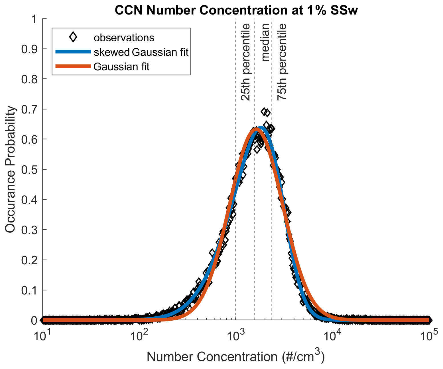
Figure 2 Distribution of CCN number concentrations active at 1 % SS_w over the course of the study. The distribution fits a skewed Gaussian model exceptionally well and an unskewed Gaussian model with moderate fidelity.

The frequency distributions of observations fit exceptionally well to skewed log-normal distributions (described in Appendix B), with low degrees of skewness, such that the log-normal distributions remain a fair approximation in many cases. Aerosol data are seldom fit in this manner, and the median and percentile bounds are simply reported instead. On the other hand, log-normal distributions have been noted and used for aerosol optical depth (AOD), either for spatial or temporal variations (Alexandrov et al., 2004, 2016; Anderson et al., 2003; Sayer and Knobelspiesse, 2019). While the methods used for AOD treatments have not been widely adopted for aerosol distributions or CCN spectra, they could be, and hopefully supplying parameterizations in the same form makes further work that is focused on the impacts of variability more accessible. Additionally, better fits for the probability distribution functions could be incorporated into microphysical modeling studies or other efforts interested in the likelihood of the given aerosol conditions occurring. When using these fit data, it is important to keep in mind that neighboring size bins are statistically correlated with each other – the probability of finding 100 particles in the 10 nm size bin is not independent of the probability of finding 100 particles in the 15 nm size bin. Because of this, the simplest way to calculate combined or correlated quantities (for example, the number concentrations of all particles between 10 and 20 nm) is through our archived distributions across time points of interest, rather than by utilizing our fit parameters. A similar skewed log-normal distribution could be fit for the combined data if desired. It should also be noted that distribution shapes may not be well conserved across all timescales or length scales. Variations are most likely to occur at small timescales (less than 2 h) or length scales (less than 0.5 km), based on the analysis discussed in Sect. 3.2 and previous works (Alexandrov et al., 2004; Anderson et al., 2003). Finally, it is important to emphasize that the uncertainties in the CCN spectra discussed in Sect. 3.1 are not necessarily reduced by this statistical fitting approach, due to their potentially systematic rather than random nature.

3.1.2 Clustering analysis

Clustering analysis is used to simplify and seek relationships in the rather large and complicated dataset. K-means clustering is performed using a vector-based distance metric. Details of the cluster analysis can be found in Appendix C. From the K-means clustering applied to the CCN spectra, three distinct clusters are identified that achieve good separation in both the CCN and size distribution characteristics, as shown in Fig. 3. The systematic uncertainties in our CCN distributions discussed in Sect. 3.1 are expected to be inherited by the characteristic cluster spectra shown here.

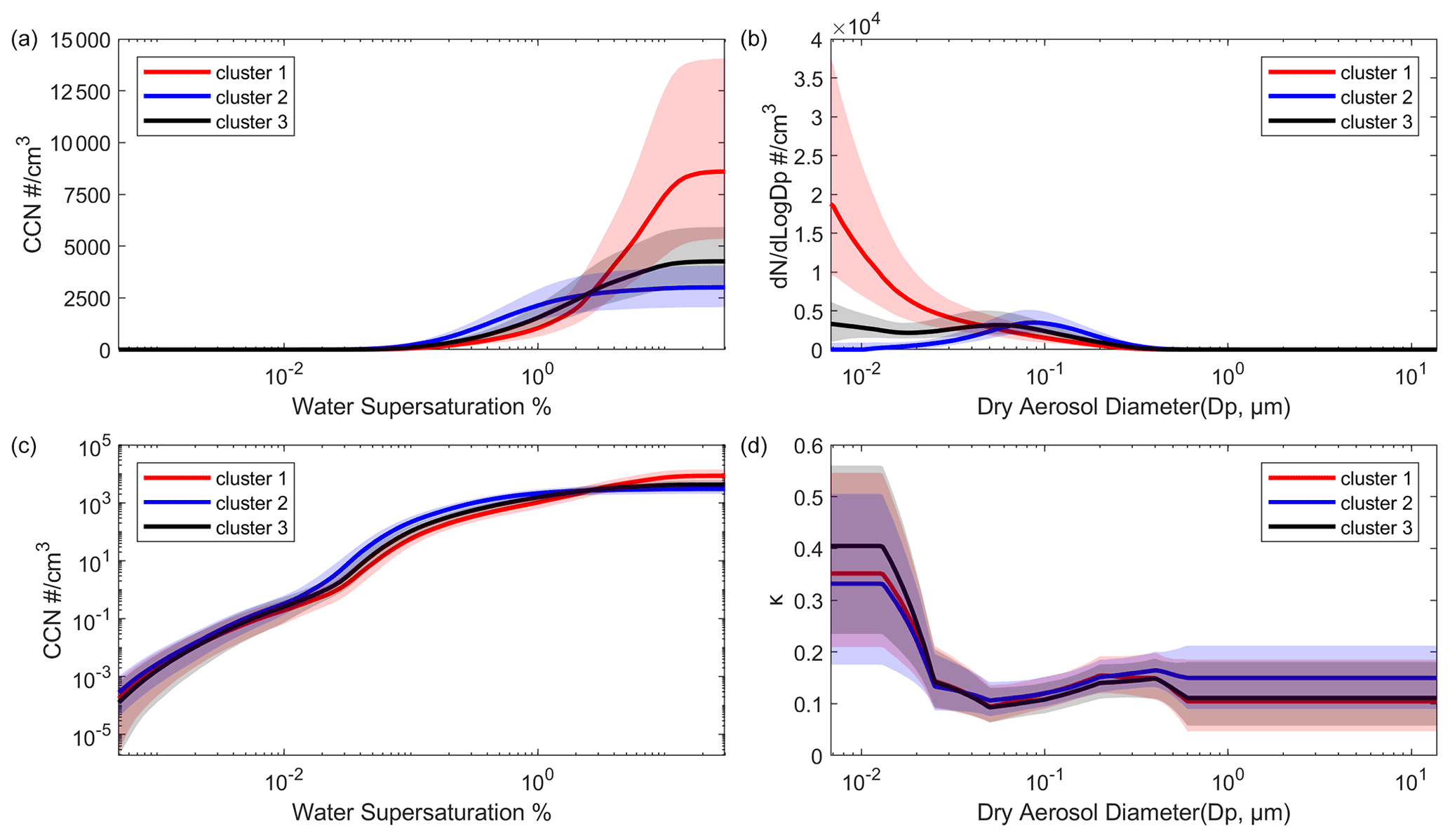
Figure 3 Clusters generated by the K-means clustering procedure. Cluster centers are shown by solid lines, with shaded region representing the 25th and 75th percentile bounds for spectra associated with each cluster. Panels (a) and (c) show the cluster CCN spectra, panel (b) shows the cluster size distributions, and panel (d) shows the cluster hygroscopicity parameter κ.

Clustering is carried out based on CCN spectra – that is, each spectrum was assigned to a cluster based on its shape and magnitude. Even though the clustering procedure had no direct information about particle size distributions, the size distributions associated with each cluster are well resolved (Fig. 3b). On the other hand, the hygroscopicity parameter distributions are similar for all three clusters (Fig. 3d). This indicates that particle size distributions have a greater influence on the resulting CCN spectra than κ distributions do, which is consistent with other analyses (Patel and Jiang, 2021). As a result, estimates of CCN spectra using size distribution data and either estimated or median κ values are expected to be reasonable approximations, although the deviations of approximate CCN spectra from observed CCN spectra can still be quite large for any given time point. We estimate the error introduced using a median κ to compute CCN spectra, as follows. For this median κ estimate, we calculated a median κ value based on the entire dataset, and then used this median value in combination with all individual size distributions to generate estimated CCN spectra. These are then compared to the CCN spectrum products (using concurrent κ and size distribution data) to calculate error estimates, with the results shown in Fig. 4. Estimates are generally least reliable for lower supersaturations, with estimates below 0.2 % SS_w having a 95 % confidence interval broader than ±50 % of the estimated value. Therefore, care should be taken when interpreting estimated CCN spectra in this low SS_w region. This highlights the region of the CCN spectrum that is most sensitive to observed variations in κ (Mahish and Collins, 2017) and the uncertainty in our data product below about 0.03 % SS_w. In this region, particles significantly larger than 600 nm are expected to activate, but we do not have accurate κ measurements for these sizes, as discussed in Sect. 2. Above 0.2 % SS_w, the median κ estimate works quite well, with uncertainties decreasing as SS_w increases. This region of the spectrum is likely a good candidate for the generation of CCN spectra from observations of particle distributions, where high-quality κ measurements are available for only a limited time period. It is important to note that this approach will only work for accurate size distribution data extending to diameters larger than 500 nm. For distributions ending at 500 nm, many CCN activating at or below ∼ 0.2 % SS_w will not be directly counted, and due to the cumulative nature of the distributions, this gap can introduce large errors for all SS_w values. We expect this median κ estimation method to be especially applicable for the SGP site and similar environments, but it may apply elsewhere as well.

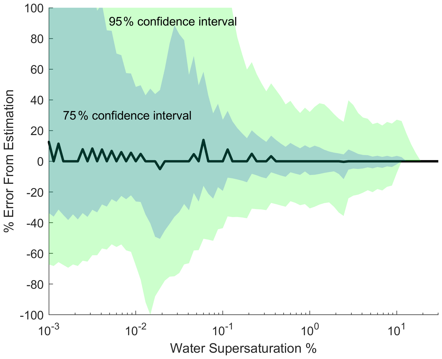
Figure 4 Error estimation of the CCN product constructed from median hygroscopicity data, as compared with that computed for size-dependent κ. The black line depicts the median error, while the dark and light green shaded regions depict 75 % and 95 % confidence intervals, respectively.

The clustering of CCN spectra into distinct groups highlights the contributions from particle size distributions as the distinguishing factor. This analysis does not suggest that κ distributions for small particles are invariant, random, or unimportant – only that their contribution to a final CCN spectrum is small compared to the contribution of the particle size distribution. Mahish and Collins (2017) provide a more complete analysis of the κ measurements at SGP during this time period, which is consistent with the data we use here.

Because of the factors discussed above, the different CCN clusters represent different characteristic particle size distributions. Cluster 1 represents cases where the nucleation mode particles, associated with new particle formation events, dominate the size distributions. Cluster 1 also has lower absolute number concentrations of accumulation mode particles than found in the other clusters. Cluster 2 represents the opposite case, i.e., the absence of small particles and higher accumulation mode number concentrations combined with a shift of the accumulation mode to larger sizes. Cluster 3 is the intermediate case, with some nucleation mode particles and a substantial accumulation mode. The three clusters represent approximately equal portions of the total number of observations. Because these clusters represent three different scenarios quite well, we will use them to simplify the further discussion. Cluster 1 will subsequently be referred to as the nucleation cluster, cluster 2 the accumulation cluster, and cluster 3 the intermediate cluster.

Figure 5 Cluster fractional likelihood for each season.

Figure 6 Diurnal variability in cluster fractional likelihood.

3.1.3 Seasonal and diurnal trends

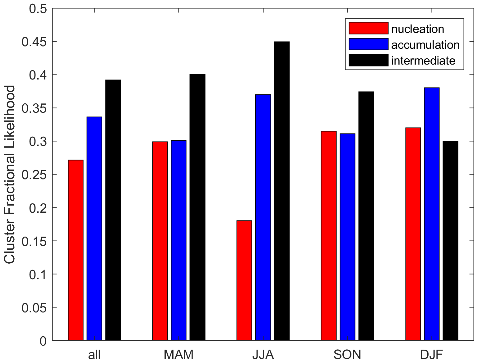
The clustered data are examined for seasonal variations in particle and CCN characteristics. Due to the differential nature of comparisons between clusters, the effect of uncertainties discussed in Sect. 3.1 is likely minimized. Cluster prevalence shows some seasonal dependence, although all clusters are still found for a significant portion of the time for all seasons (Fig. 5). Summer (July–August; JJA) and winter (December–February; DJF) seasons show the highest prevalence of accumulation clusters but significant differences in fractions of the intermediate and nucleation clusters. Summer has the highest prevalence of the intermediate clusters, while winter has the highest prevalence of nucleation clusters. This suggests that, during the summer, significant particle concentrations are more likely to coexist in both the accumulation and nucleation modes, or perhaps that the growth of nucleation mode particles to larger sizes (i.e., transfer of particles to the accumulation mode) is more likely to occur. These trends are not obvious from looking at seasonal particle data alone (Marinescu et al., 2019). An important consideration for reconciling seasonal particle data, as discussed in Marinescu et al. (2019), and seasonal cluster trends is the fact that the distributions within a cluster will have seasonal dependence as well, as shown in Fig. C1.

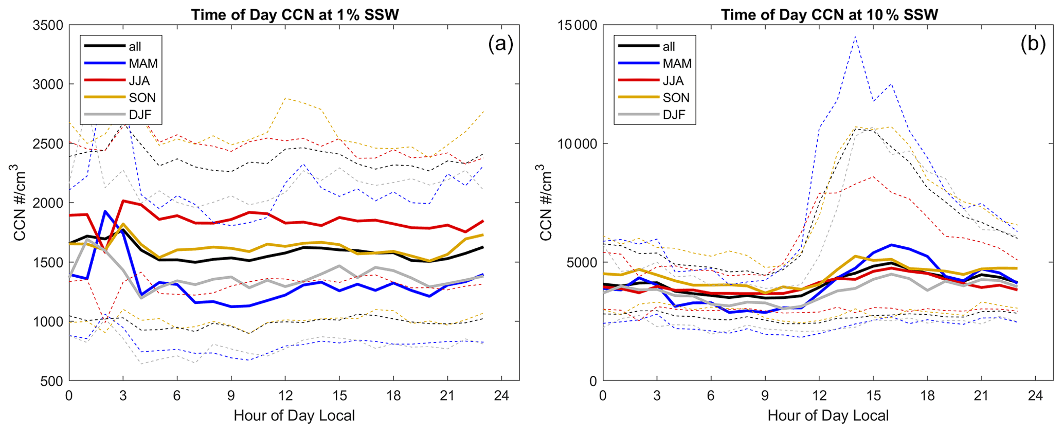
Figure 7 Median (solid lines) and 75 % confidence intervals (dotted lines) with seasonally averaged CCN concentrations at 1 % (a) and 10 % (b) SS_w, as a function of the local time of day.

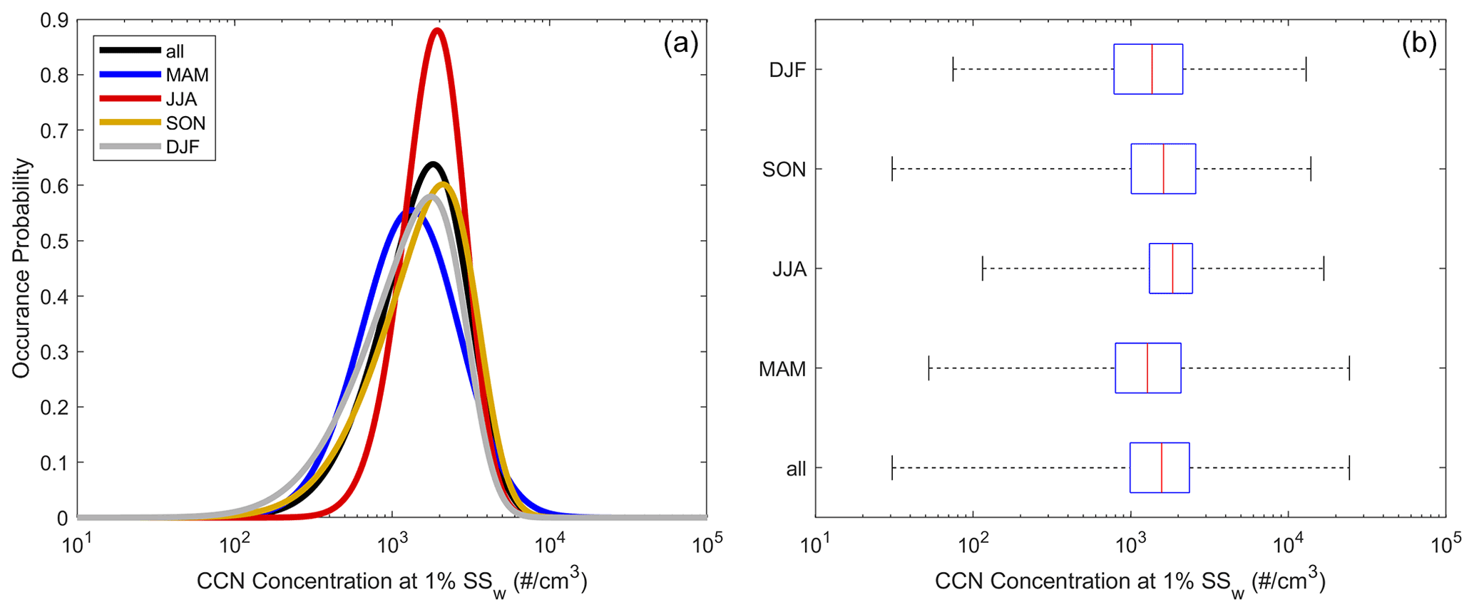
Figure 8 Distributions of the CCN concentrations at 1 % SS_w separated seasonally, using skewed log-normal fits (a) and box plots (b).

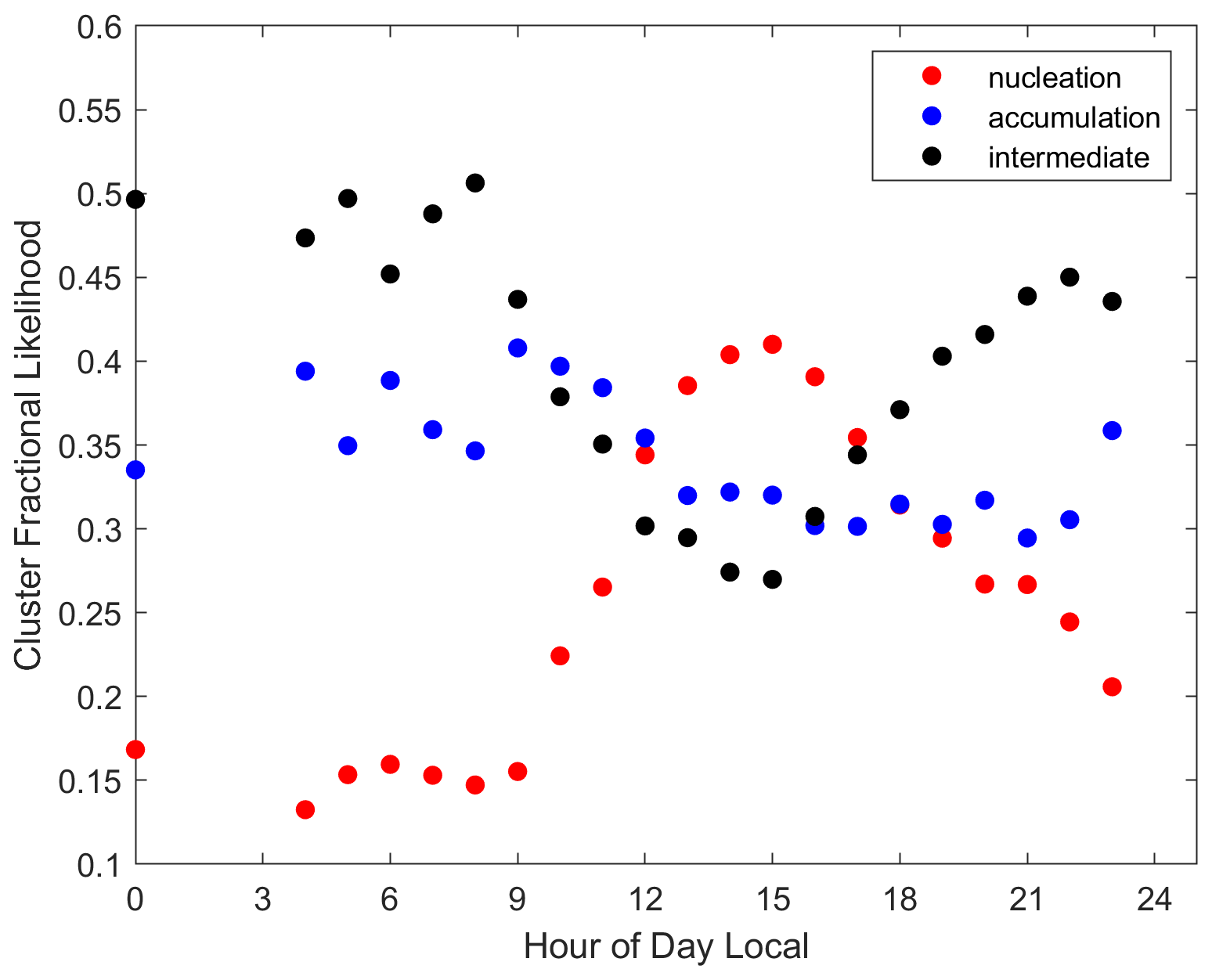
Figure 6 depicts how cluster prevalence changes as a function of the time of day. Nucleation mode clusters are most common during daylight hours, with intermediate clusters most likely at night. Interestingly, accumulation clusters show the least time dependence over the course of the day. Analysis of CCN concentrations at several supersaturations, as shown in Fig. 7, shows no hourly dependence in median values at 1 % SS_w or lower. At 10 % SS_w, the hourly trend in CCN is similar to the hourly trend in the nucleation cluster. These data combined suggest that the hourly changes that occur are due to the addition of nucleation mode particles rather than changes in the particle concentrations of other modes. The seasonal variability in the nucleation mode time-of-day dependence is shown in Fig. C1 and reflects the same overall time dependence within a day, alongside the seasonal changes shown in Fig. 5.

Another way to examine the seasonal changes is through a comparison of the occurrence probabilities at a single supersaturation, as shown in Fig. 8. Figure 8 shows this information in two similar ways, namely with the skewed log-normal fits from Sect. 3.1.1 and Appendix B and more traditional box plots. Both methods of parameterizing the data require the same number of parameters (three coefficients, a zero fraction, and a correlation coefficient for the fit; there are five points for the box and whiskers), but the fits convey more information. Seasonal differences are somewhat obscured by the box plot, but, for cumulative CCN active at 1 % supersaturation, a clear difference between the summer months and the rest of the year is observed with the fits, where CCN concentrations are more tightly grouped at higher values in the summer. Fit parameters for all supersaturations and seasons can be found in the Supplement (supporting file CCN_fit_coeffs.txt). The fits derived for cumulative CCN active at high supersaturations (1 % and higher) are relevant to cases of deep convection, whereas those derived for very low supersaturations (below 0.1 %) may be helpful for estimates of the abundances of particles in special populations such as giant CCN.

3.2 Time evolution of clusters

Our large dataset allows for additional statistical analysis to examine the evolution of CCN spectra over time. This gives insight into the underlying processes that are obscured when examining single cases or shorter data periods. Figure 9 shows the evolution of cluster classifications over time, examining all clusters starting in a given classification (nucleation, accumulation, or intermediate). Cluster classification changes for all three clusters on the timescale of hours. Nucleation clusters are most likely to transition to intermediate clusters, rather than going directly to accumulation clusters. This could be through any or all of the following: growth of nucleation mode aerosol into larger sizes, coagulation scavenging-, deposition-, or evaporation-induced loss of the nucleation mode, and changes in air mass. Similarly, accumulation mode clusters are also more readily transitioned to intermediate clusters than to nucleation clusters. The role of intermediate clusters as the pathway of conversion between accumulation and nucleation clusters is further reinforced by the fact that they are equally likely to transition to either cluster type. In terms outside of the clustering perspective, it appears most likely that transitions from aerosol distributions dominated by nucleation mode particles to ones dominated by accumulation mode particles (or vice versa) occur smoothly through intermediate cases where both modes are of similar magnitude, rather than doing so abruptly. However, the analysis cannot distinguish the specific role of meteorology in these transitions.

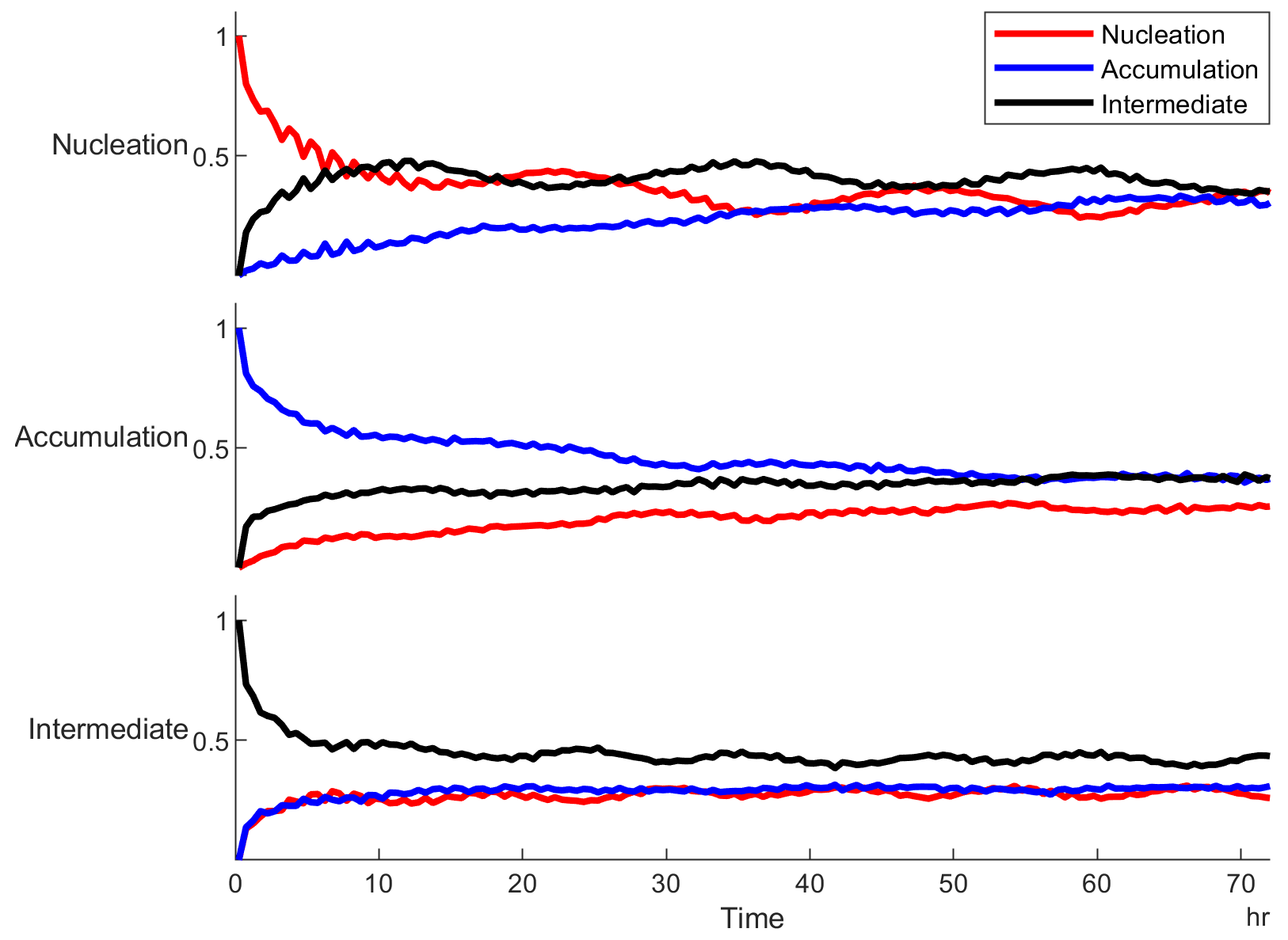
Figure 9 Cluster evolution over time (hours after the appearance of a cluster). The y axis for each plot shows the likelihood of the cluster transitioning to a new cluster type after a specified time, while the x axis has elapsed. The first collection of traces labeled nucleation shows the evolution of the nucleation cluster spectra into the other categories, with the middle collection depicting the evolution of accumulation cluster initial states and the bottom showing evolution of intermediate cluster initial states. Traces indicate the final states (after the specified time lag) of the nucleation cluster (red), accumulation cluster (blue), or intermediate cluster (black).

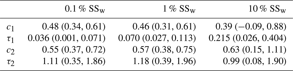
There is some periodicity observed in the cluster evolution, which we examine more closely alongside fluctuations in CCN number concentrations using autocorrelations. Autocorrelation coefficients are calculated for several different SS_w conditions, as shown in Fig. 10, using the methods described in Appendix D. Autocorrelation coefficients can be interpreted similarly to other correlation coefficients – they describe that portion of the variance that can be explained by the observation at a previous time point. Because of the differential nature of these comparisons, uncertainties in CCN distribution discussed in Sect. 3.1 are unlikely to propagate into this analysis. Furthermore, the regions of highest uncertainty are avoided here. The higher the value of an autocorrelation coefficient, the more stable that quantity is over time, so that an autocorrelation coefficient of 1 implies no change in state at a specified time lag, while 0 implies that a previous data point (separated by the specified time lag) has no influence on a current one. From Fig. 10, a great deal of variability is observed in the first several hours of the computed time lags, which is an unexpected finding. Autocorrelation coefficients are expected to be highest for the first several time points, but the oscillating nature of these points implies aerosol processes with some periodicity in the 2–3 h range. Natural processes that might produce such variability throughout the day and over all seasons seem unlikely, so the oscillation may be an artifact, for example, introduced by sampling schedules. We apply a bi-exponential fit as an approximate way to smooth the data for time lags of up to 12 h, removing the effect of these oscillations. Single exponential fits are poor approximations of the shape of the autocorrelation functions for 0.1 % and 1 % SS_w cases. Because a single decay pathway is expected to produce relatively consistent decay rates, the appearance of multi-exponential decays suggests multiple decay pathways. In this case, decay pathways for autocorrelation can be interpreted as pathways for changes in CCN number concentrations.

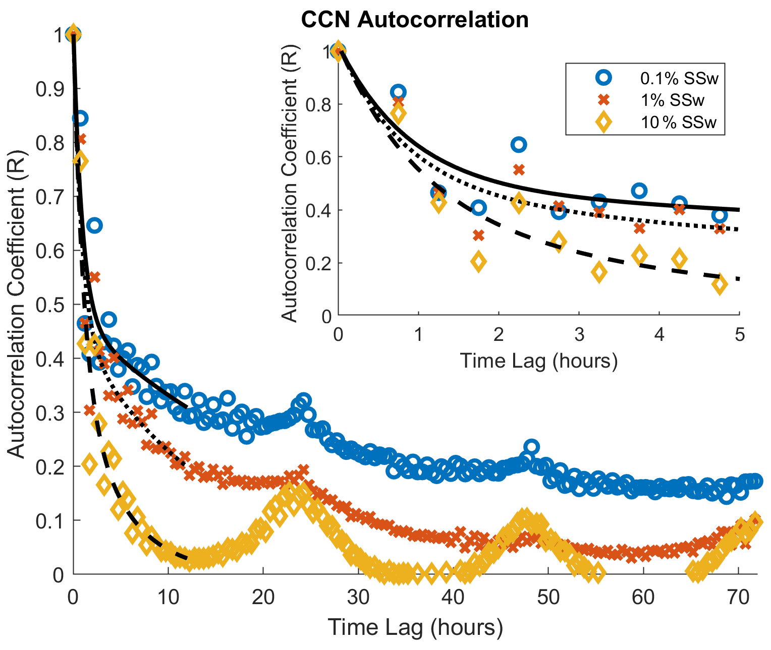
Figure 10 Autocorrelation functions for CCN number concentrations at variable SS_w. Bi-exponential fits are shown for the first 12 h of lag time for each SS_w, with solid, dotted, and dashed lines corresponding to 0.1 %, 1 %, and 10 % SS_w, respectively.

Autocorrelation decays much more quickly for larger (10 %) SS_w, with greatly increased values appearing at 24 h intervals. At higher SS_w, the CCN number concentration is often dominated by the smallest particles, which are associated with the nucleation mode. This interpretation fits well with the autocorrelation data, which indicate short-lived events tied to diurnal cycles. At moderate (1 %) and low (0.1 %) SS_w, there is a pronounced fast initial decay in autocorrelation, followed by a period of slower decay. Fit constants are described in Appendix D and shown in Table D1. The fast initial decay rate is comparable (within the large uncertainties; Table D1) for low and moderate SS_w cases, but the slow decay rate is significantly slower for the low SS_w case. The diurnal peak (at 24 h time lag) is also significantly weaker for the lowest SS_w case, suggesting that there is less variability in these lowest SS_w CCN observations, as compared to higher SS_w. This is consistent with the fact that number concentrations at larger particle sizes are much less variable than those at smaller particle sizes (Marinescu et al., 2019). Previous work on AOD spatial and temporal autocorrelation at the SGP site (Alexandrov et al., 2004) and elsewhere (Anderson et al., 2003) suggest that the fast decay can be attributed to 3D microscale turbulent fluctuations, while the slow decay is due to 2D large-scale turbulence. The aerosol data used here are obtained only at the surface, so the influence of the three-dimensional nature of the atmosphere may be present but cannot be distinguished. Given the role of new particle formation events, there is also potentially a chemical (non-turbulence-driven) source of variability for CCN, contributing to the autocorrelation decay for CCN concentrations at high SS_w. Ultimately, these data illustrate that CCN spectra change rapidly over 1–3 h timescales, with some conservation at longer timescales for the lower end of the supersaturation range. The granularity of our data (in ∼ 45 min increments) makes it somewhat difficult to resolve the exact timescales, but it is clear that the period of rapid change is in the 1–3 h range. The role of variability in CCN concentration is something that should be considered in modeling studies that focus on the impacts of aerosol, especially those that use fixed concentrations of aerosol particles or those that do not capture the comprehensive processes that cause aerosol concentrations and properties to evolve. For example, using fixed CCN concentrations for a given short-term (< 2 h) simulation of shallow clouds (i.e., lower supersaturations) is more justifiable than for a longer-term simulation of the development of deep convective clouds (i.e., higher supersaturations), based on the faster autocorrelation decay rates of CCN at higher supersaturations. The autocorrelation results can also help to define the timescales for data assimilation to ensure models are updated frequently enough to allow for accurate simulations.

4 Conclusions

We have developed, described, and examined a long-term CCN spectrum data product for the SGP site in Oklahoma. The data product builds on merged size distributions (Marinescu et al., 2019) and hygroscopicity measurements (Mahish and Collins, 2017) to create a best estimate of CCN spectra across a wide supersaturation range from ∼ 0.0001 % to 30 %. It has been generated and verified by combining high quality data from seven different instruments. It has ∼ 45 min temporal resolution across 5 years of data, from 2009 to 2013, which has allowed for analyses not normally possible for smaller datasets.

We have determined that skewed log-normal distributions provide excellent fits to occurrence probabilities of CCN concentrations at any given supersaturation and to occurrence probabilities of a wide range of other aerosol quantities. These types of distributions have been observed for AOD measurements previously but have not been widely used. They provide more information than traditional box plots, while requiring a comparable number of parameters. For established occurrence distribution shapes, shorter timescale measurements could likely take advantage of these fit parameters to fill in data gaps to estimate data over longer periods. They also serve as useful inputs to models that include the expected variability in input parameters in model predictions.

CCN spectra are controlled primarily by particle size distributions, especially at larger SS_w values (above ∼ 0.2 %). In this high SS_w region of the spectrum, it appears possible to generate estimated CCN spectra using only median κ values, rather than concurrent measurements of κ and size distribution. However, this estimation relies on accurate size distribution data that extend beyond 500 nm. Approximations of uncertainties introduced by this median κ estimation have been investigated and should hold for data from the SGP site during different time periods. This estimation method is also likely applicable for other sites, especially in similar environments, but is beyond the scope of this analysis.

Clustering analysis also highlights size distributions as the driving force behind changes in CCN spectra. There are three distinct clusters that have been found for cases dominated by nucleation mode particles, accumulation mode particles, or similar amounts of each. These are analyzed seasonally and hourly, finding all clusters in significant quantities across all seasons and times. Intermediate clusters are more likely during the summer months, while accumulation clusters are abundant in the winter. Fall and spring appear similar in this view, falling between summer and winter. Nucleation mode clusters are most likely during daylight hours, corresponding with decreased intermediate clusters but nearly invariant accumulation clusters.

Time evolutions are examined in this dataset to try to understand the dynamics of CCN spectra. Analysis of transitions between clusters reveals that the most likely path is for nucleation and accumulation mode clusters to transition to an intermediate cluster first, rather than to direct transitions occurring between the two. Autocorrelation analyses probe the evolution of a given CCN SS_w bin over time. A relatively quick decay is found for all SS_w values, with the bulk of the correlation decaying in several hours, indicating that relatively large changes in CCN spectra can be expected over that time period. An additional slow decay is observed for smaller SS_w values, indicating that the CCN number is better conserved at longer timescales (> 2–3 h) in lower SS_w regions of the CCN spectrum, corresponding to particles in the coarse mode.

Appendix A: Merging of distributions and CCN spectra

The initial size distributions used in this work are generated from a combination of scanning mobility particle sizer (SMPS), aerodynamic particle sizer (APS), and condensation particle counter (CPC) data, as described previously by Marinescu et al. (2019), which are available in the DOE ARM archive (Marinescu and Levin, 2019). This initial dataset, here referred to as size distribution (SD) 1, is processed to take into account additional instrument data utilizing humidified tandem differential mobility analyzer (HTDMA), CCN counter (CCNC), nephelometer, and aerosol chemical speciation mass spectrometer (ACSM) instrument data, as outlined in Fig. A1. SD1 data are available in approximately ∼ 45 min time intervals, where additional instrument data are available in a higher time resolution and are subsequently averaged over the time period of SD1 data for comparison. In order to compare to CCNC measurements, SD1 must be converted to CCN spectra using the hygroscopicity parameter (κ) that is derived from HTDMA measurements.

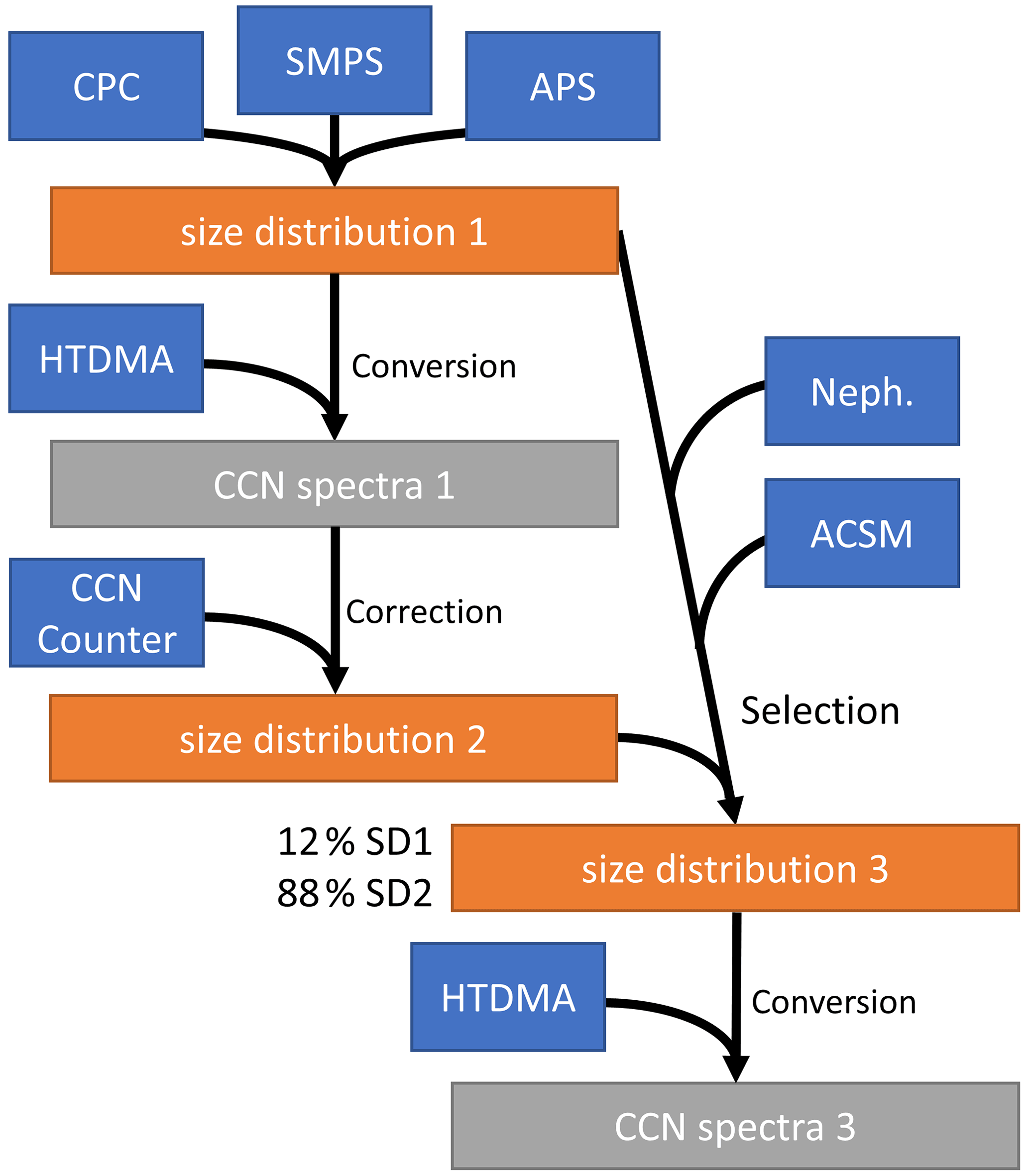
Figure A1 Flowchart illustrating the processing of data to various distributions, with input instrument data shown in blue boxes, size distributions in orange, and CCN spectra in gray.

Size-resolved aerosol hygroscopicity was measured with a HTDMA (Collins, 2010b), which first selected dried, mono-disperse aerosol at seven diameters and then exposed them to a humidified (relative humidity – RH ∼ 90 %) growth region. The humidified aerosol size distribution was then measured, and the change in particle diameter between the selected dry particle diameter (D_p) and the resulting humidified size (D_w) is termed the growth factor (GF = $D_{\mathrm{w}}/D_{\mathrm{p}})$. An example of HTDMA measured growth factor distributions is shown in Fig. A2. The orange lines indicate the selected dry size for each GF measurement. The top part of the figure shows the size distribution measured by the SMPS at the same time.

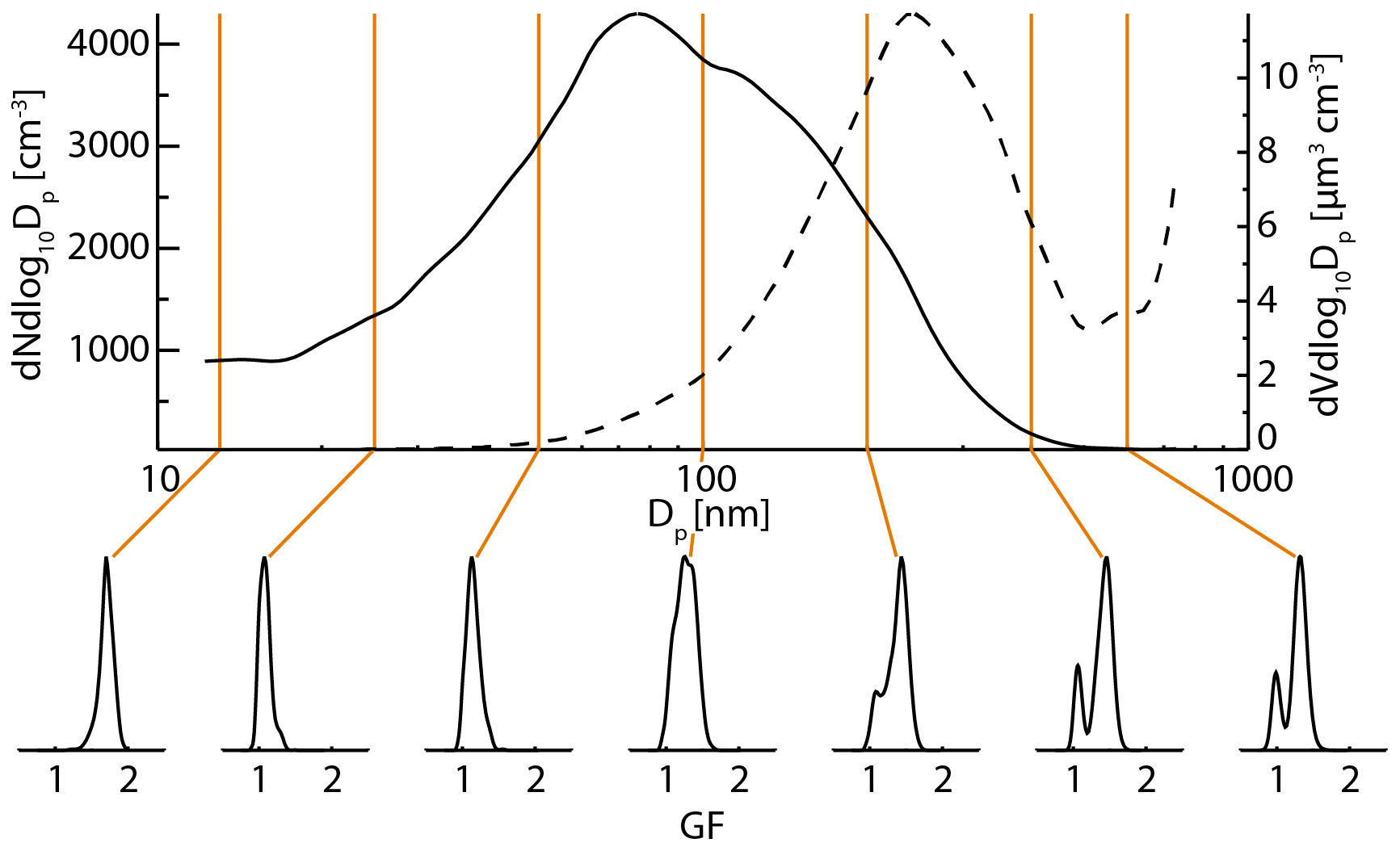
Figure A2 Example aerosol number distribution (solid line; upper plot) and growth factor (at 90 % RH) distributions (lower plots) measured by an HTDMA. The dashed line in the upper plot is the corresponding volume distribution.

These GF data at a given RH (properly written as, e.g., GF(90 %), but abbreviated here to GF for convenience) can be used to calculate the hygroscopicity of the particles, as expressed via the hygroscopicity parameter, κ, in the following (Carrico et al., 2010; Petters and Kreidenweis, 2007):

$$\begin{array}{}\text{(A1)}& \mathit{\kappa }={\displaystyle \frac{\left({\mathrm{GF}}^{\mathrm{3}}-\mathrm{1}\right)\left(\mathrm{1}-a_{\mathrm{w}}\right)}{a_{\mathrm{w}}}},\end{array}$$

where

$$\begin{array}{}\text{(A2)}& a_{\mathrm{w}}={\displaystyle \frac{\mathrm{RH}}{\exp \left(\frac{\mathrm{4}{\mathit{\sigma }}_{\mathrm{w}}{M}_{\mathrm{w}}}{{\mathit{\rho }}_{\mathrm{w}}RT{D}_{\mathrm{d}}\mathrm{GF}}\right)}},\end{array}$$

and σ_w, M_w, and ρ_w are the surface tension, molecular weight, and density of water, respectively, T is the absolute temperature, and R is the ideal gas constant. After calculating κ distributions from each measured GF distribution at the diameters selected by the HTDMA, we averaged κ for each selected D_d and linearly interpolated between selected sizes to generate a continuous distribution of aerosol hygroscopicity across the entire size distribution. Given the uncertainties introduced by interpolation and extension of κ data beyond measurement bounds, we believe any added uncertainty introduced by using the average κ rather than a κ distribution is relatively minor.

CCN spectra were generated using these κ values, derived from the HTDMA growth factor data described above using either the SD1 (initial) or SD3 (final) size distributions (described below). For each time period with concurrent κ and size distribution data, critical SS_w was calculated for each size bin. This was accomplished using Eqs. (A1) and (A2), assuming the following constant conditions: temperature of 25 ^∘C, water density of 1 g mL⁻¹, and surface tension of 72 mJ m⁻². This calculation is accomplished numerically, by calculating water SS_w for a logarithmically spaced array of wet diameters, with the largest SS_w chosen as the critical value. Calculated errors from this method were less than 1 % of the calculated values using this method (e.g. a 1 % error in a 0.01 % SS_w being ±0.0001 % SS_w). A CCN spectrum was then generated by adding up the activated particle populations at each SS_w value, making no assumptions about the order particles activated in; smaller particles with higher κ could activate before large particles with low κ, if appropriate.

In order to compare spectra between CCN spectrum 1 and measured CCNC values averaged across the same ∼ 45 min time intervals, interpolation of the CCNC data across the calculated SS_w bins was performed using MATLAB's built-in piecewise cubic hermite interpolating polynomial (PCHIP) function for each CCNC spectrum. These data were used to create a distribution corrected for the CCNC data using a similar method to that described for the CPC corrections in SD1 (Marinescu et al., 2019). The only difference between the algorithm described in Appendix A of Marinescu et al. (2019) and the one used for generation of SD2 here occurs in step 3. We calculated a 2-week rolling median percent difference between the CPC and SMPS + APS distribution and used this as a scaling factor across the entire distribution in this step. Times between 12:00 and 18:00 LT are excluded from the rolling median since new particle formation events are common during those times and large differences between the SMPS + APS integrated number concentration and the CPC number concentration are expected. To generate SD2, the average difference between CPC and CCNC (in total, particles and SS_w specific CCN numbers, respectively) is used instead of solely using CPC data. For example, if the comparison with the CPC suggested that there should be 25 % more particles in the SMPS + APS size distributions, and the comparison with the CCNC suggested there should be 15 % fewer particles in the SMPS + APS size distributions, then the SMPS + APS size distribution data are scaled up by 5 % (the average of +25 % and −15 %). The remaining steps described in Marinescu et al. (2019) are performed unchanged on this distribution. The remaining steps in the algorithm can change the shape of the size distribution, so SD1 and SD2 are not simply scaled versions of each other. If no quality CCNC data are available for a given time point, the SD1 and SD2 spectra are identical.

The resulting SD2 was then compared to ACSM and nephelometer data to examine whether the CCNC correction was warranted. ACSM comparisons were accomplished by generating total particle mass concentration for each distribution, assuming spherical particles and a density of 1.77 mg mL⁻¹, which is that of ammonium sulfate. Additionally, the ACSM cutoff of 1 µm and the volume equivalent diameter (DeCarlo et al., 2004) were accounted for to produce the calculated aerosol mass for comparison. The density chosen is within the region of best agreement between the ACSM and distribution data for both the SD1 and SD2 and is chosen for consistency with the nephelometer comparison. The nephelometer comparison was accomplished by generating single particle scattering cross-sections for all size bins in the distributions assuming the optical properties of ammonium sulfate, which was again within the region of best agreement in Fig. A3. Both of these comparisons produce excellent agreement for many time points, as shown in Fig. A4. There was evidence of systematic bias for some time periods but the bias was relatively low for periods outside of 10 March 2011 through 1 November 2011 for the nephelometer data, which were not used in distribution selection below.

SD2 generally produced a better agreement with the nephelometer and ACSM than SD1 did, although this was not true for all time periods. In order to construct a final dataset including the nephelometer and ACSM comparisons, the ratios between distribution-calculated values and measured values were used to select between SD1 and SD2 at each point where data were available. Given the better general agreement for SD2, it was used as default if there were no ACSM or nephelometer data available, or if there was disagreement between the two instruments. Through this process, 4711 distributions were selected from SD1 and 16203 from SD2, with 19407 points defaulting to SD2. The resulting distribution, of SD3 compared with ACSM and nephelometer measurements in Fig. A3, is considered to be the final product distribution and analyzed throughout the paper alongside the CCN spectra generated from it.

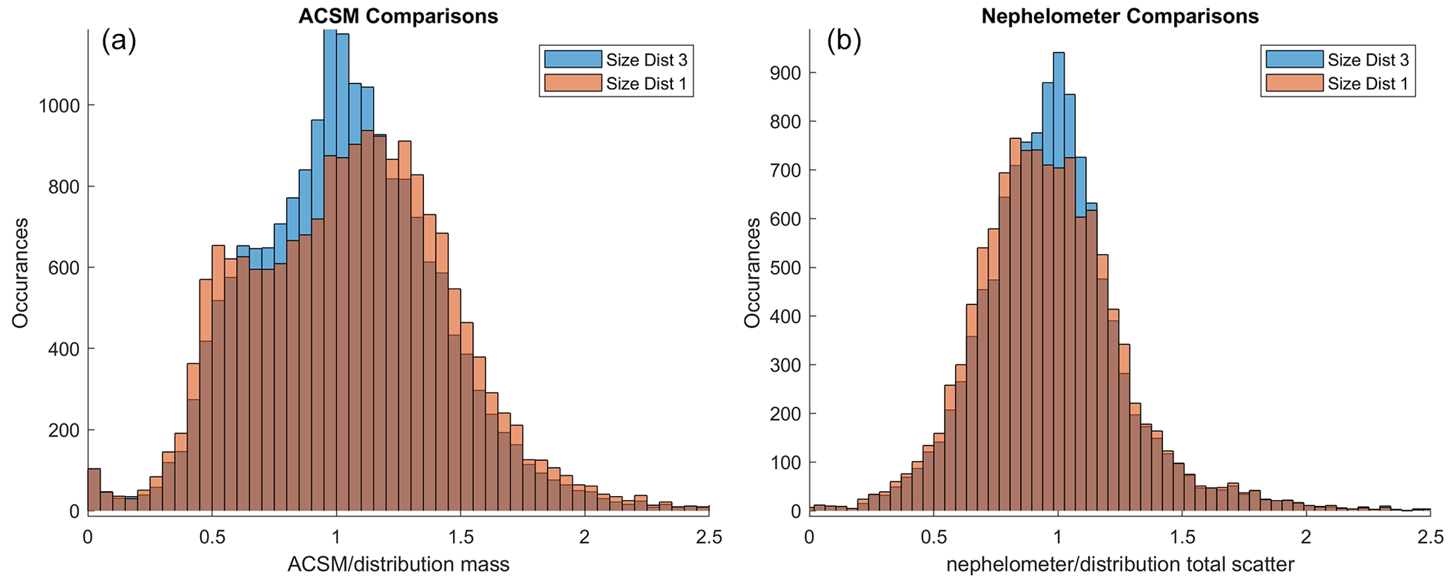
Figure A3 Statistical comparisons of the agreement between measured quantities (a is ACSM aerosol mass concentrations; b is PM₁₀ nephelometer scattering coefficients) and those estimated from either the SD1 or SD3 size distributions. The x axes show the comparisons as ratios, where a ratio of 1 indicates perfect agreement.

Figure A4 Examples of excluded (a) and included (b) nephelometer data (blue traces) compared to total scattering coefficients calculated from the indicated estimated size distributions (SD1 or SD3).

Appendix B: Skewed log-normal fits

The log-normal probability density function is defined as follows:

$$\begin{array}{}\text{(B1)}& \mathit{\phi }\left(\ln x\right)={\displaystyle \frac{\mathrm{1}}{x\mathit{\sigma }\sqrt{\mathrm{2}\mathit{\pi }}}}\exp \left(-{\displaystyle \frac{(\ln x-\mathit{\mu }{)}^{\mathrm{2}}}{\mathrm{2}{\mathit{\sigma }}^{\mathrm{2}}}}\right),\end{array}$$

where x is a number concentration (bin), μ is the median value of log(x), and σ² is the variance in log(x). The log-normal cumulative distribution function is defined as follows:

$$\begin{array}{}\text{(B2)}& \mathrm{\Phi }\left(\ln x\right)={\displaystyle \frac{\mathrm{1}}{\mathrm{2}}}+{\displaystyle \frac{\mathrm{1}}{\mathrm{2}}}\mathrm{erf}\left[{\displaystyle \frac{\ln x-\mathit{\mu }}{\mathit{\sigma }\sqrt{\mathrm{2}}}}\right],\end{array}$$

where erf is the error function. A skewed log-normal probability density function can subsequently be defined as follows:

$$\begin{array}{}\text{(B3)}& f\left(\ln x\right)=\mathrm{2}\mathit{\phi }\left(\ln x\right)\mathrm{\Phi }\left(\mathit{\alpha }\ln x\right),\end{array}$$

where α is a parameter representing the degree of skewness, such that, when α= 0, then the log-normal distribution is recovered. When these functions are used to fit data, μ, σ, and α are used as the fit parameters.

There are two issues that arise when using skewed log-normal fits. The first is that there is no closed-form expression for the median value of a skewed log-normal distribution. The median can, of course, still be evaluated numerically. The second is that x values of zero cannot be represented within the distribution due to the logarithm. In this work, we address these issues by simply reporting the median values and fractions of the data where zeros occur, alongside the fit parameters. It should be noted μ is no longer the median value of log(x) for the skewed log-normal distribution. This can be observed in the data in the Supplement (supporting file CCN_fit_coeffs.txt), where μ decreases at high SS_w, while the median value increases monotonically, as expected for a cumulative distribution. Fits are generally very good, as shown in Fig. B1 for several different aerosol quantities. At very low SS_w, or for very large particle bins, the quality of the fits degrades due to the large amount of noise in the data. This noise occurs largely due to the detection limits of the instruments involved at low particle concentrations (for very large particles). If concentrations are so low that the particle detections are not guaranteed in the sampling period (45 min), a large amount of shot noise is introduced.

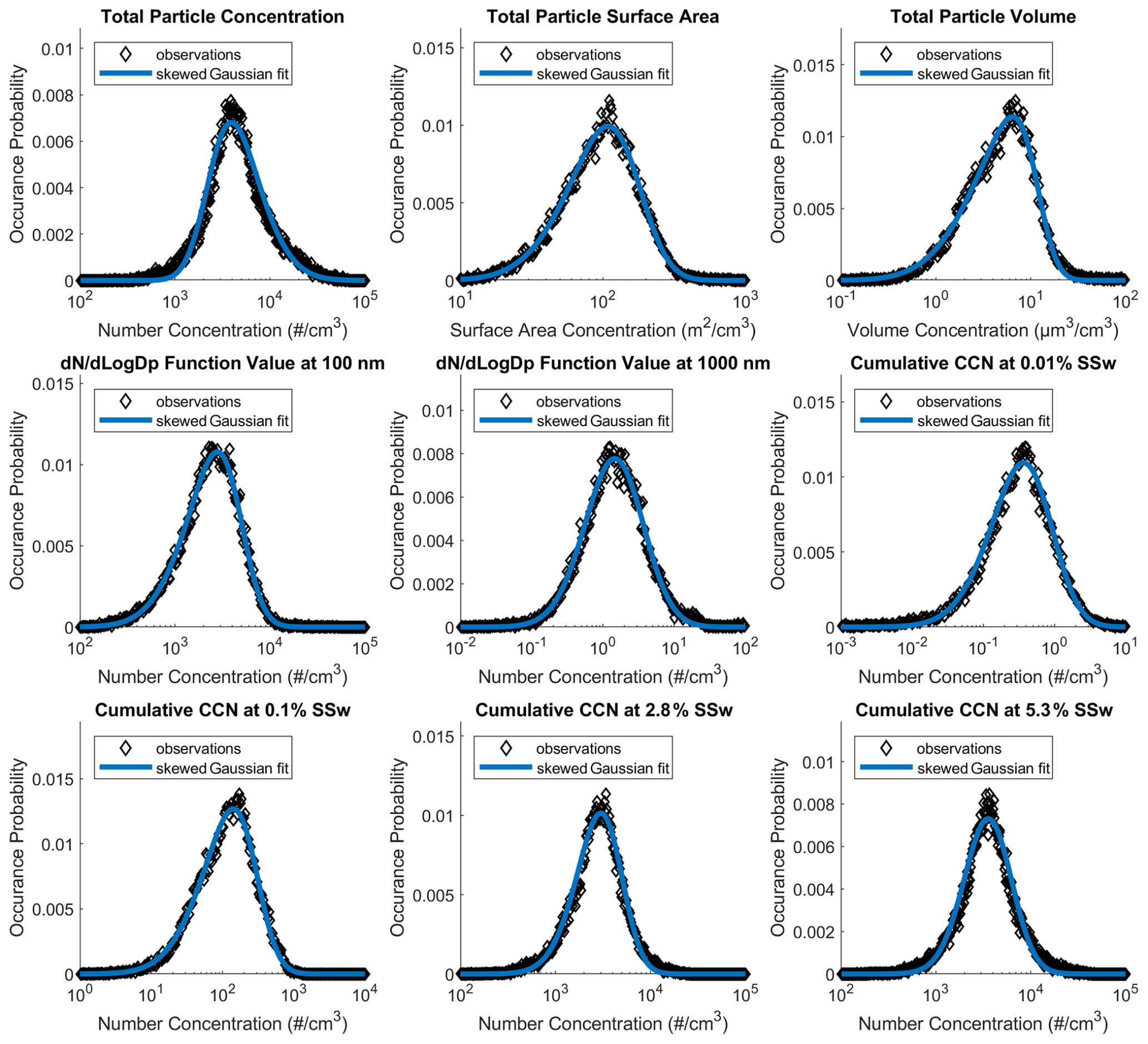
Figure B1 Examples of skewed log-normal fits to occurrence probabilities for aerosol metrics are labeled as follows: total particle number, total particle volume, dN $/$ dLogD_p function at 100 nm, dN $/$ dLogD_p function at 1000 nm, and particle number concentrations active as CCN at 0.01 %, 0.1 %, 2.8 %, and 5.3 % SS_w.

Appendix C: Clustering analysis

Clustering was done after evaluating several different methods and options. The primary parameters that were varied were the number of clusters used, and the distance metric used to distinguish clusters. All analysis was performed using the built-in MATLAB functions. There were three distance metrics evaluated using the K-means function options, i.e., the (1) squared Euclidian, (2) sum of absolute differences (city block), and (3) cosine. Each option defines cluster distance, d, as follows:

$$\begin{array}{}\text{(C1)}& {\displaystyle }{d}_{\mathrm{1}}\left(x,c\right)=(x-c)(x-c{)}^{\prime }\text{(C2)}& {\displaystyle }{d}_{\mathrm{2}}\left(x,c\right)=\sum _j\left|x_j-c_j\right|\text{(C3)}& {\displaystyle }{d}_{\mathrm{3}}\left(x,c\right)=\mathrm{1}-{\displaystyle \frac{x{c}^{\prime }}{\sqrt{\left(x{x}^{\prime }\right)\left(c{c}^{\prime }\right)}}},\end{array}$$

where x is input data (CCN spectrum for a given time point), and c is a cluster centroid. Both x and c are arrays, with subscripts indicating a single array element and apostrophes indicating a transpose operation. It was found that metrics 1 and 2 produced the separation of spectra based solely on the total particle number, depending on whether clustering was applied to aerosol size distributions or to CCN spectra. Distance metric 3, however, produced well-resolved clusters, based on the distribution shape (how the CCN spectrum changes with SS_w), and was selected for final cluster designations. Mathematically, distance metric 3 is a measure of the included angle between points treated as vectors, which provides some effective normalization, so the result of the clusters based on the distribution shape rather than total aerosol number is not surprising. Clustering in the CCN space also produced well-resolved clusters in the size distribution space and vice versa. The CCN space was ultimately chosen for clustering, due to the focus of the current work, but differences from the alternative are expected to be very minor.

Next, the optimal number of clusters was explored. While this is often accomplished somewhat arbitrarily, intuitively, or based on external models for a given process, statistical methods have been developed to guide the process. We chose to use the gap statistic (Tibshirani et al., 2001), a built-in MATLAB functionality, through the evalclusters function. This method was too computationally intensive to use on the entire dataset, so a subset of 500 randomly selected spectra were used instead. There were three clusters that were suggested to be the optimal number to use, based on this approach. These clusters all appeared to be physically distinct, as discussed in Sect. 3.1.2, and the addition of a fourth cluster simply resulted in the splitting of two adjacent clusters. The three clusters were thus chosen for use in further analysis.

Clusters are generally similar year-round, but there is some seasonal dependence within a given cluster, as shown in Fig. C1.

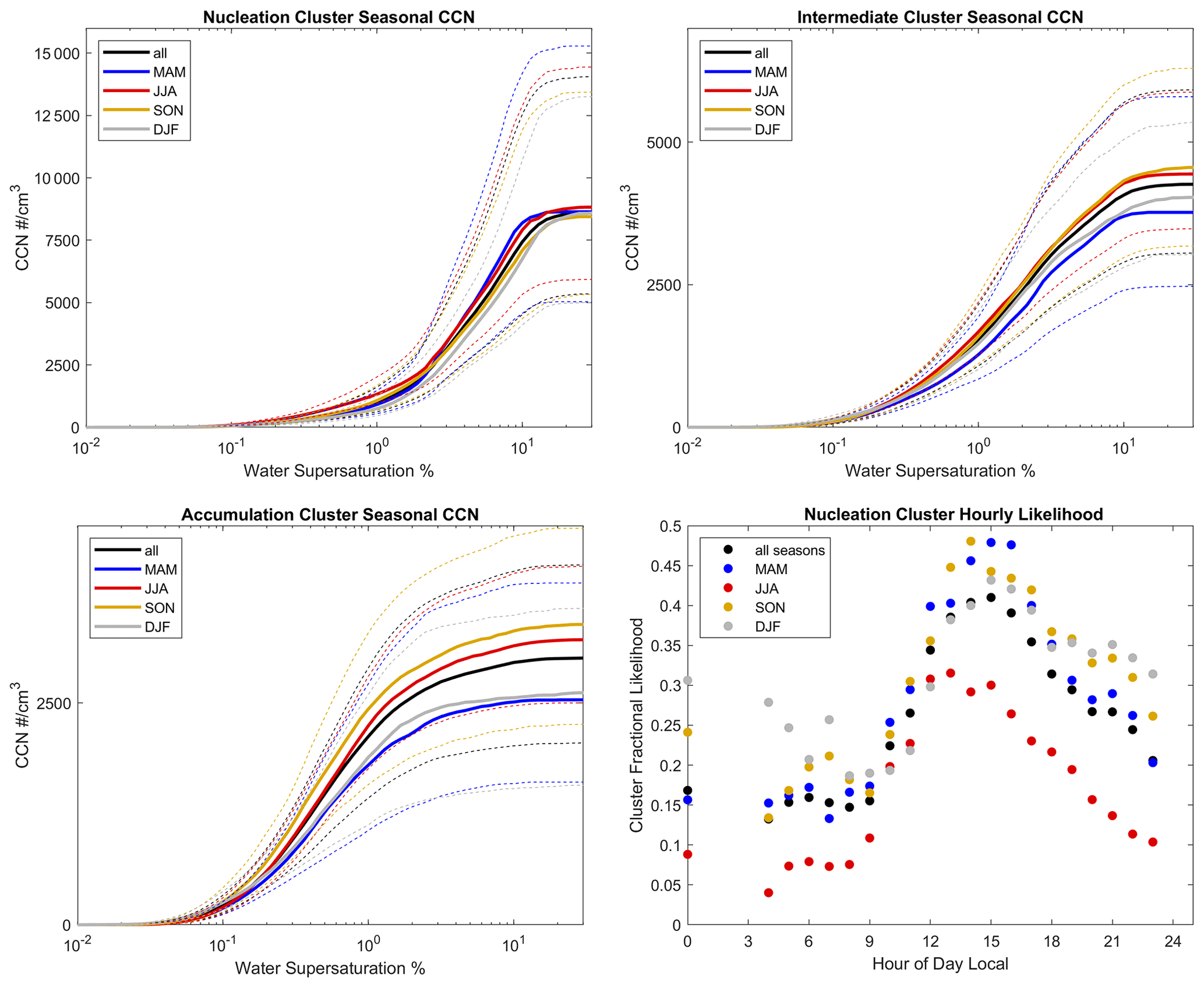
Figure C1 Median (solid lines) and confidence intervals containing 75 % of the data (dotted lines) for each cluster as a function of the season, along with seasonal variations in hourly cluster likelihood for the nucleation mode cluster (bottom right).

Appendix D: Non-periodic autocorrelation and fits

Autocorrelation coefficients (Box et al., 2015) were generated by comparing adjacent points in a time series to determine the portion of variance that can be explained by the adjacent points. For a time series with equally spaced measurements, the autocorrelation function is defined as follows:

$$\begin{array}{}\text{(D1)}& r_k={\displaystyle \frac{{\sum }_{i=\mathrm{1}}^{N-k}(Y_i-\stackrel{\mathrm{‾}}{Y})(Y_{i+k}-\stackrel{\mathrm{‾}}{Y})}{\sum _{i=\mathrm{1}}^N(Y_i-\stackrel{\mathrm{‾}}{Y}{)}^{\mathrm{2}}}},\end{array}$$

where r_k is the autocorrelation coefficient at time lag k, N is the total number of time points, Y_i is the measurement value (in our case CCN number concentration) at time point i, and $\stackrel{\mathrm{‾}}{Y}$ is the mean measurement value. For time points that are not evenly spaced, the same coefficient can be produced with a few extra steps. The way we have accomplished this is to (1) calculate the differences between all adjacent time points, for a fixed number of integer time lags, before (2) sorting all of these data into time bins based on how much time elapsed between any given set of measurements.

Autocorrelation functions were subsequently fit to bi-exponential decays for the first 12 h of time lag data, using the following form:

$$\begin{array}{}\text{(D2)}& f\left(x\right)=c_{\mathrm{1}}{e}^{-{\mathit{\tau }}_{\mathrm{1}}x}+c_{\mathrm{2}}{e}^{-{\mathit{\tau }}_{\mathrm{2}}x}.\end{array}$$

This is accomplished using the fit function in MATLAB, which provides the 95 % confidence interval information. Best fit parameters and 95 % confidence intervals are reported in Table D1 below.

Table D1 Bi-exponential fit coefficients.