the Creative Commons Attribution 4.0 License.
the Creative Commons Attribution 4.0 License.
 | 11 May 2022
Tropospheric ozone production and chemical regime analysis during the COVID-19 lockdown over Europe
Clara M. Nussbaumer
Andrea Pozzer
Ivan Tadic
Lenard Röder
Florian Obersteiner
Hartwig Harder
Jos Lelieveld
Horst Fischer
The COVID-19 (coronavirus disease 2019) European lockdowns have led to a significant reduction in the emissions of primary pollutants such as NO (nitric oxide) and NO2 (nitrogen dioxide). As most photochemical processes are related to nitrogen oxide (NOx≡ NO + NO2) chemistry, this event has presented an exceptional opportunity to investigate its effects on air quality and secondary pollutants, such as tropospheric ozone (O3). In this study, we present the effects of the COVID-19 lockdown on atmospheric trace gas concentrations, net ozone production rates (NOPRs) and the dominant chemical regime throughout the troposphere based on three different research aircraft campaigns across Europe. These are the UTOPIHAN (Upper Tropospheric Ozone: Processes Involving HOx and NOx) campaigns in 2003 and 2004, the HOOVER (HOx over Europe) campaigns in 2006 and 2007, and the BLUESKY campaign in 2020, the latter performed during the COVID-19 lockdown. We present in situ observations and simulation results from the ECHAM5 (fifth-generation European Centre Hamburg general circulation model, version 5.3.02)/MESSy2 (second-generation Modular Earth Submodel System, version 2.54.0) Atmospheric Chemistry (EMAC), model which allows for scenario calculations with business-as-usual emissions during the BLUESKY campaign, referred to as the “no-lockdown scenario”. We show that the COVID-19 lockdown reduced NO and NO2 mixing ratios in the upper troposphere by around 55 % compared to the no-lockdown scenario due to reduced air traffic. O3 production and loss terms reflected this reduction with a deceleration in O3 cycling due to reduced mixing ratios of NOx, while NOPRs were largely unaffected. We also study the role of methyl peroxyradicals forming HCHO () to show that the COVID-19 lockdown shifted the chemistry in the upper-troposphere–tropopause region to a NOx-limited regime during BLUESKY. In comparison, we find a volatile organic compound (VOC)-limited regime to be dominant during UTOPIHAN.
- Article
(3249 KB) - Full-text XML
-
Supplement
(1101 KB) - BibTeX
- EndNote


COVID-19 (coronavirus disease 2019) describes the disease accompanying an infection with the SARS-CoV-2 (severe acute respiratory syndrome coronavirus-2) virus. The disease is highly infectious and can have severe health consequences, including premature death, particularly for the elderly and people with pre-existing conditions (WHO, 2021). On 11 March 2020, COVID-19 was declared a pandemic by the World Health Organization (WHO, 2020a, b). As a response, in many countries worldwide – including the European continent – governments initiated a shutdown of the daily life for minimizing the spread of the virus, which is referred to as a COVID-19 lockdown. Among others, this included a reduction in vehicular and industrial activities as well as sharp restrictions on air travel accompanied by a reduction in atmospheric pollutants such as nitrogen oxides () (Venter et al., 2020; Kroll et al., 2020; Chossière et al., 2021; Onyeaka et al., 2021; Salma et al., 2020; Matthias et al., 2021; Forster et al., 2020).
NO and NO2 are important atmospheric trace gases as they are involved in almost all photochemical processes taking place in the earth's atmosphere. NOx directly impacts the production of tropospheric ozone (O3), which is a hazard to human and plant health (Nuvolone et al., 2018; Mills et al., 2018). Together with volatile organic compound (VOC) oxidation, NO forms NO2 within the HOx cycle, catalyzed by an OH radical. Under the influence of sunlight, NO2 can subsequently form O3 through the reaction with molecular oxygen, as shown in Reaction (R1) (Leighton, 1971; Crutzen, 1988; Lelieveld and Dentener, 2000; Pusede and Cohen, 2012; Pusede et al., 2015; Nussbaumer and Cohen, 2020).
Various termination reactions such as the formation of HNO3 from OH and NO2 or other radical recombinations cause ozone chemistry to be non-linear, which means that a reduction in ambient NOx can either increase or decrease O3 production (Calvert and Stockwell, 1983; Pusede et al., 2015). For low ambient NOx levels, a NOx reduction usually causes a decrease in O3 production, which is referred to as a NOx-limited chemical regime. In contrast, a NOx reduction increases O3 production when a VOC-limited chemical regime is dominant – usually at high ambient NOx levels (Sillman et al., 1990; National Research Council, 1992; Pusede and Cohen, 2012). In the transition region between the two regimes, changes in NOx do not (or only slightly) impact O3 production rates (Wang et al., 2018). Earlier studies on evaluating correlations of NOx and O3 in the troposphere include Liu et al. (1987), Logan (1985) and Lin et al. (1988), reporting a non-linear dependence that varies with ambient levels of hydrocarbons and NOx.
Many different methods enable the determination of the dominant chemical regime, such as the use of the weekend ozone effect, which considers the response of O3 to NOx reductions on weekends, or the ratio of HCHO to NO2, with various approaches from in situ observations, remote sensing and model simulations (e.g., Jin et al., 2020; Pusede and Cohen, 2012; Nussbaumer and Cohen, 2020; Duncan et al., 2010). We have recently shown that the fraction α of methyl peroxyradicals (CH3O2) forming formaldehyde (HCHO) in correlation with ambient NO concentrations is capable of indicating the dominant chemical regime based on three different field campaigns across Europe in Finland (HUMPPA 2012), Germany (HOPE 2012) and Cyprus (CYPHEX 2014) (Nussbaumer et al., 2021). CH3O2 formed from, for example, the oxidation of acetaldehyde (CH3CHO) or methane (CH4) can either react with NO or OH radicals to form HCHO or undergo the competing reaction with HO2 to form methyl hydroperoxide (CH3OOH). For more details, please see Fig. 1 in Nussbaumer et al. (2021). consequently depends on the ambient concentrations of NO, OH and HO2 and the respective rate constants for the reaction with CH3O2, the latter of which were taken from the IUPAC Task Group on Atmospheric Chemical Kinetic Data Evaluation (2021). Self-reaction of CH3O2 as a contributor to CH3O2 loss forming HCHO is negligible. The calculation of is presented in Eq. (1).
Low values for with a high response to NO are an indicator for a NOx-limited regime, whereas high values for with little response to changing NO represent a VOC limitation (Fig. 11 in Nussbaumer et al., 2021). Investigating the dominant chemical regime is an important method for analyzing photochemical processes and air quality.
Previous studies have explored changes in air quality, trace gas emissions and the dominant chemical regime during the COVID-19 lockdown in Europe. Menut et al. (2020) reported NO2 reductions between 30 % and 50 % for various western European countries in the course of March 2020, with both decreasing and increasing O3 concentrations in response, depending on the location, based on surface in situ observations and model simulations. Ordóñez et al. (2020) observed decreased NO2 and increased O3 concentrations in central Europe in March and April 2020 based on in situ observations compared to 2015–2019. While they found NO2 reductions to be mainly attributed to the COVID-19 lockdown, O3 enhancements were predominantly affected by meteorological changes. Chossière et al. (2021) presented evidence of NO2 reductions during the COVID-19 lockdown in Europe and O3 changes dependent on the dominant chemical regime through investigation of ratios based on in situ and satellite observations. Similar studies were performed by Matthias et al. (2021), Mertens et al. (2021), Balamurugan et al. (2021), Grange et al. (2021) and many more.
Besides the changes within the dominant chemical regime through NOx reductions, i.e., increasing ozone within a VOC-limited regime and decreasing ozone within a NOx-limited regime, the COVID-19 lockdown could have potentially changed the dominant chemical regime from VOC- to NOx-limited as pointed out by Kroll et al. (2020) and Gaubert et al. (2021). Cazorla et al. (2021) found a lockdown-induced change from a VOC- to a NOx-limited regime in Quito (Ecuador) based on the share of precursor loss to HNO3 and H2O2. The latter is dominant for NOx-limited chemistry (Kleinman et al., 2001). A change from a VOC- to a NOx-limited regime was also reported by Zhu et al. (2021) in China based on HCHO-to-NO2 ratios (NOx limitation for ratios above 2 according to Duncan et al., 2010).
Most of the literature on pollutant reductions during the COVID-19 lockdown focuses on near-surface air quality, and only few studies consider the free troposphere. Steinbrecht et al. (2021), Chang et al. (2022) and Bouarar et al. (2021) reported decreases in O3 concentrations in the free troposphere based on in situ observations and modeling studies in the Northern Hemisphere. Bouarar et al. (2021) found that reduced air traffic – a unique incidence after strongly increasing aircraft activities over the past decades, as shown by Lee et al. (2021) – can explain around a third of the observed O3 decrease in 2020, the remaining contributions coming from ground-level reductions and meteorological differences. Reduced O3 in the free troposphere was also reported by Clark et al. (2021) around Frankfurt airport. Cristofanelli et al. (2021) reported lower O3 concentrations above the planetary boundary layer (PBL) in 2020 compared to the 1996–2019 average at Monte Cimone in Italy, which is in line with findings by the World Meteorological Organization (2021), extended to include two mountain sites in Germany.
In this study, we present atmospheric trace gas concentrations, net ozone production rates and an analysis on the dominant chemical regime based on in situ observations during the research aircraft campaign BLUESKY, which took place in May and June 2020 over Europe, and model simulations. During this time period, aircraft activity was still strongly limited due to the COVID-19 lockdown. We compare the results to model simulations assuming business-as-usual emissions not impacted by government restrictions, which we refer to as the “no-lockdown scenario”. Additionally, we present results of two previous aircraft campaigns, which are UTOPIHAN (Upper Tropospheric Ozone: Processes Involving HOx and NOx) in 2003/04 and HOOVER (HOx over Europe) in 2006/07. While many studies have been published on emissions reductions and the effect on secondary pollutants during the COVID-19 lockdown, only a few studies have investigated changes in the dominant chemical regime, and to our knowledge we are the first to report a shift to NOx-limited chemistry in the upper troposphere. This can demonstrate the consequences of emission changes in VOCs (including methane) and NOx for tropospheric ozone.
2.1 Calculations of net ozone production rates (NOPRs)
Besides the chemical regime, production and loss processes of O3 are effective tools in exploring relevant photochemistry. As already demonstrated in Reaction (R1), O3 is formed via NO2 photolysis. Under the assumption of photostationary state, this term can be equated with the reactions of NO with O3, HO2 and RO2 (Hosaynali Beygi et al., 2011). The resulting term for O3 production P(O3) is shown in Eq. (2) (Tadic et al., 2020; Leighton, 1971); j(NO2) is the photolysis frequency of NO2, and k describes the respective rate constant (for this work taken from the IUPAC Task Group on Atmospheric Chemical Kinetic Data Evaluation, 2021).
We assume RzO2 (the sum of all peroxy radicals) to be represented by CH3O2, which we find to be a reasonable approximation when comparing modeled CH3O2 to the overall modeled RO2 as shown in Fig. S1 in the Supplement, exemplarily for the BLUESKY campaign. Above 800 hPa, CH3O2 represents more than 90 % of RO2. Below 800 hPa, it still accounts for more than 70 % on average. CH3O2 can be calculated via Eq. (3) as derived by Bozem et al. (2017a). While the model can simulate CH3O2 mixing ratios, Eq. (3) is required when working with experimental data as CH3O2 was not directly measured.
O3 loss occurs via the reaction with NO, OH and HO2 and via photolysis and can be calculated as presented in Eq. (4). The photolysis of O3 first yields O1D, which reacts back to O3 through collision with O2 or N2 and causes an O3 loss through reaction with H2O. The share of O3 that is effectively lost through O3 photolysis is described by in Eq. (5) (Bozem et al., 2017a). Additional loss due to reactions of O3 with alkenes and the loss of NO2 due to formation of HNO3 or peroxy nitrates are negligibly small, particularly in the upper troposphere.
Net ozone production rates (NOPRs) are then calculated from the difference in P(O3) and L(O3), whereas P(O3) can be expressed via either NO2 or NO reaction terms. The term can be neglected for the latter as it is equally present in P(O3) and L(O3).
2.2 Field experiments
We have investigated in situ trace gas observations from three different research aircraft campaigns, which are the UTOPIHAN campaigns in 2003/04, the HOOVER campaigns in 2006/07 and the BLUESKY campaign in 2020. Figure 1 shows an overview of the flight tracks over Europe. We have filtered the data for the tropospheric region with the help of the modeled tropopause pressure (see Sect. 2.3) and south of 60∘ N as there were no data points for the BLUESKY campaign further north. Dashed lines show the complete flight tracks during each campaign, and solid lines show the data which we have considered in this study. The experimental data were obtained with a time resolution of 1 min and subsequently adjusted to fit the model resolution of 6 min. For this, each sixth experimental data point (which fit the model timescale) and the data points from ±2 min were averaged. The remaining data points were discarded.
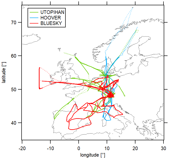
Figure 1Overview of the flight tracks of the considered aircraft campaigns: UTOPIHAN (2003 and 2004) in green, HOOVER (2006 and 2007) in blue and BLUESKY (2020) in red. Solid lines present the data considered in this study (filtered for troposphere and south of 60∘ N), and dashed lines show the complete flight tracks.
2.2.1 UTOPIHAN 2003/04
The UTOPIHAN (Upper Tropospheric Ozone: Processes Involving HOx and NOx) campaigns took place in June/July 2003 and March 2004 starting from Oberpfaffenhofen airport in Germany (48.08∘ N, 11.28∘ E) with the GFD (Gesellschaft für Flugzieldarstellung, Hohn, Germany) research aircraft Learjet 35A (Colomb et al., 2006; Klippel et al., 2011; Stickler et al., 2006). NO and O3 were measured via chemiluminescent detection (CLD 790 SR, ECO Physics, Dürnten, Switzerland). NO data have a precision of 6.5 %, an accuracy of ≤25 % and a detection limit of <0.01 ppbv. O3 data have a precision of 1 % and an accuracy of 5 %; j(NO2) was determined via filter radiometers (Meterologie Consult GmbH, Königstein, Germany) with a precision of 1 % and an accuracy of 15 %. CO measurements were obtained from a tunable diode laser absorption spectrometer with a detection limit of 0.26 ppbv (30 s time resolution) and an accuracy of 3.6 % (6 s time resolution) (Kormann et al., 2005).
2.2.2 HOOVER 2006/07
The HOOVER (HOx over Europe) campaigns took place in October 2006 and July 2007 using the GFD research aircraft Learjet 35A with the campaign base in Hohn, Germany (54.31∘ N, 9.53∘ E) (Klippel et al., 2011; Bozem et al., 2017b, a; Regelin et al., 2013). NO and O3 measurements were performed via chemiluminescence (CLD 790 SR, ECO Physics, Dürnten, Switzerland) with a precision of 7 % and 4 %, an accuracy of 12 % and 2 %, and a detection limit of 0.2 and 2 ppbv, respectively (30 s time resolution) (Hosaynali Beygi et al., 2011). CO and CH4 were measured via quantum cascade laser absorption spectroscopy with an accuracy of 1.1 % and 0.6 % and detection limits of 0.2 and 6 ppbv, respectively (2 s time resolution) (Schiller et al., 2008). OH and HO2 measurements were performed via laser-induced fluorescence with the HORUS (HydrOxyl Radical measurement Unit based on fluorescence Spectroscopy) instrument with an accuracy of 18 % and detection limits of 0.016 and 0.33 pptv, respectively (1 min time resolution) (Regelin et al., 2013). Photolysis frequencies were measured using filter radiometers (Meterologie Consult GmbH, Königstein, Germany) with a precision of 1 % and an accuracy of 15 % (1 s time resolution). H2O was measured via IR absorption with a typical accuracy of 1 % (modified LI-6262, LI-COR Inc., Lincoln, USA) (Gurk et al., 2008; LI-COR, Inc., 1996).
2.2.3 BLUESKY 2020
The BLUESKY campaign took place in May and June 2020 over Europe. Eight flights were carried out using the HALO (High Altitude Long Range) research aircraft starting from the campaign base in Oberpfaffenhofen, Germany. The goal of the campaign was to examine the effects of the COVID-19 lockdown on the troposphere and lower stratosphere over European cities, rural areas and the transatlantic flight corridor. More details can be found in Reifenberg et al. (2022) and Voigt et al. (2022). While most restrictions across Europe were in place in March and April 2020, May and June emissions, particularly from air travel but also from ground-based sources such as on-road traffic, were still affected by the COVID-19 lockdowns (Schlosser et al., 2020; Brockmann Lab, 2022; Hasegawa, 2022; EUROCONTROL, 2022). NO was measured via chemiluminescence (CLD 790 SR, ECO Physics, Dürnten, Switzerland) with a total uncertainty of 15 % and a detection limit of 5 pptv (1 min time resolution) (Tadic et al., 2020).
O3 measurements were performed with the FAIRO (Fast AIRborne Ozone) instrument, which allows fast detection via chemiluminescence that is calibrated in situ by UV photometry (2.5 % combined uncertainty, 5 Hz time resolution) (Zahn et al., 2012). CO was measured via the quantum cascade laser spectrometer TRISTAR (Tracer In Situ TDLAS for Atmospheric Research) with an uncertainty of 3 % (1 min time resolution) (Schiller et al., 2008).
2.3 Modeling study
The modeled data were obtained from the ECHAM5 (fifth-generation European Centre Hamburg general circulation model, version 5.3.02)/MESSy2 (second-generation Modular Earth Submodel System, version 2.54.0) Atmospheric Chemistry (EMAC) model, which is described in Jöckel et al. (2016) and Reifenberg et al. (2022).
We use data of NO, NO2, O3, OH, HO2, CO, CH4, CH3O2, H2O, j(NO2), j(O1D) temperature and pressure, modeled along the flight tracks of the described research aircraft campaigns UTOPIHAN, HOOVER and BLUESKY. The data were filtered for the troposphere using the modeled tropopause pressure. Stratospheric data were discarded. In order to evaluate the impact of reduced emissions during the COVID-19 lockdown, the model was used to simulate a scenario with usual emissions for the BLUESKY campaign, which we refer to as the “no-lockdown scenario”. For details of the model setup please see the paper by Reifenberg et al. (2022).
This analysis is structured as follows: as a full set of in situ observations necessary for a regime analysis and calculating net ozone production rates, which includes NO, O3, OH, HO2, CO, CH4, H2O, j(NO2) and j(O1D), is only available for the HOOVER campaign, we first show that the model and experimental data are in close agreement for this campaign. We conclude from this finding that the model is generally capable of reproducing the experimental data and therefore use the model data in our following analysis. In the second step, we provide a comparison between the three campaigns as well as the no-lockdown scenario regarding the individual trace gases and net ozone production rates. We finally present our results of the analysis of the dominant chemical regime, based on .
3.1 Comparison of the model and experiment
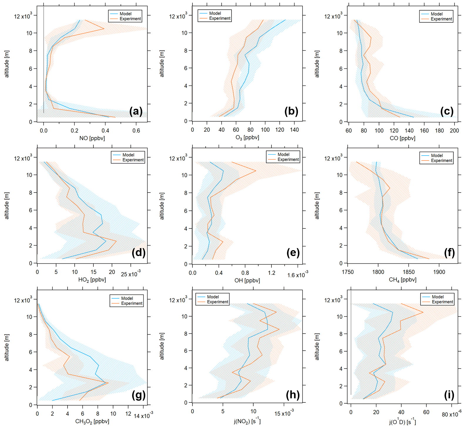
Figure 2Vertical profiles of in situ observations and model data of the atmospheric trace gases (a) NO, (b) O3, (c) CO, (d) HO2, (e) OH, (f) CH4 and (g) CH3O2 and the photolysis rates (h) j(NO2) and (i) j(O1D) during the HOOVER campaign for estimating the model performance. Blue colors show modeled data by EMAC along the HOOVER campaign flight track (model) and orange colors show experimental data (experiment). The orange trace in panel (g) shows the calculation of CH3O2 from experimental CH4, CO and HO2 via Eq. (3). The shaded areas represent the 1σ standard deviation from averaging the data points at each altitude bin. The numbers of data points averaged per altitude bin are displayed in Tables S1 and S2 in the Supplement.
Figure 2 shows a comparison of in situ observations (orange) and model simulations (blue) for the HOOVER campaign as vertical profiles. The shaded areas present the 1σ standard deviations, and the numbers of data points available for each altitude bin are shown in Tables S1 and S2 in the Supplement.
Figure 2a presents the vertical profile of NO, which shows the typical tropospheric C-shape distribution with the highest values at the surface (e.g., vehicle and industrial emissions) and the upper troposphere (e.g., aircraft and lightning emissions). Ground-level mixing ratios (0–1000 m) were around 0.4 ppbv and decreased with altitude to values of 37±27 (1σ) pptv and 47±32 pptv for the model and the experiment, respectively, between 3 and 9 km altitude. The only relevant deviation between the model and experiment was between 10 and 11 km altitude with mixing ratios of 0.20±0.03 ppbv and 0.39±0.32 ppbv, respectively.
Figure 2b shows the measured and modeled O3 mixing ratios, which were lowest at ground level, with 43.7±14.5 ppbv and 36.4±12.8 ppbv for the model and experiment and increased with altitude up to 128.1 ± 22.7 ppbv and 97.5 ± 15.6 ppbv, respectively. Model values were approximately 20 % higher compared to the measured data but showed the same vertical shape. The observed positive O3 bias of the modeled data is an issue almost all global models suffer from in the Northern Hemisphere and which has not been entirely understood yet (Revell et al., 2018; Young et al., 2018; Jöckel et al., 2016; Parrish et al., 2014).
CO vertical profiles are shown in Fig. 2c and were highest at the surface, with 146.4 ± 63.2 ppbv and 128.0 ± 42.3 ppbv for the model and experiment, respectively, and decreased with altitude to around 70 ppbv in the upper troposphere. HOx () is presented in Fig. 2d and e. HO2 mixing ratios showed a maximum value of around 20 pptv between 2 and 3 km altitude and decreased aloft to values of around 2 pptv in the upper troposphere. The model and experiment showed close agreement. OH mixing ratios were mostly below 1 pptv. Similar to NO, the main deviation between the model and experiment was between 10 and 11 km altitude, where measured values were higher by around 0.5 pptv. Nevertheless, the error bars representing the 1σ standard deviation of the averages overlapped at all altitudes.
Figure 2f shows the vertical profiles of CH4, which did not show any particular gradient with altitude. Mixing ratios were 1809 ± 19 ppbv for the model simulation and 1815 ± 40 ppbv for the experiment throughout the campaign. CH4 is needed for calculating CH3O2 via Eq. (3), which we show in Fig. 2g in orange compared to the model simulation of CH3O2. Figure 2h and i present the photolysis frequencies j(NO2) and j(O1D), which show close agreement for the model and experiment. We show the vertical profiles for H2O, temperature and pressure in Fig. S2. Again, model simulation can represent the experimental data well.
For the UTOPIHAN and the BLUESKY campaigns only a limited number of observations are available. Similar to the HOOVER campaigns, NO, O3 and CO can be well approximated by the model simulations, which we present in Figs. S3 and S4. Tropospheric ozone is slightly overestimated, which we attribute to the simplified representation of multiphase chemistry (clouds) in the present model version, which underpredicts chemical ozone loss (Rosanka et al., 2021). Based on these results, we conclude that the model is generally capable of representing the in situ observations well and use the model data for all following analyses.
3.2 Campaign comparison
3.2.1 Trace gases

Figure 3Vertical profiles of the atmospheric trace gases (a) NO, (b) O3, (c) CO, (d) NO2, (e) HO2 and (f) OH for the campaigns UTOPIHAN (green), HOOVER (blue) and BLUESKY (red) and the no-lockdown (NL) scenario (yellow). All data shown here are from EMAC model simulations along the flight track of each research campaign. Two separate simulations were run on the flight path of BLUESKY, one with lockdown and one with business-as-usual emissions. The shaded areas represent the 1σ standard deviation from averaging the data points at each altitude bin. The numbers of data points averaged per altitude bin are displayed in Table S2.
Figure 3 presents the vertical profiles of some selected trace gases during the research aircraft campaigns UTOPIHAN (green), HOOVER (blue) and BLUESKY (red) which were obtained from model simulations. Yellow lines show the no-lockdown (NL) scenario for the BLUESKY campaign in 2020.
The vertical profiles of NO are presented in Fig. 3a. For all campaigns, we observe the typical C shape as described for the HOOVER campaigns in Sect. 3.1. Surface (0–1000 m) mixing ratios were similar for UTOPIHAN and HOOVER, with 0.45±0.37 (1σ) ppbv and 0.43 ± 0.74 ppbv, respectively. In comparison, the ground-level concentration of NO during BLUESKY was 0.12 ± 0.11 ppbv. The differences in NO mixing ratios between the campaigns are the outcome of the general emission reduction due to legislative limitation of nitrogen oxides and other hazardous pollutants over the past decades as the campaigns took place 15–20 years apart. We show the decrease in NOx emissions in the model over the past 2 decades in Fig. S5. Assuming the no-lockdown scenario during BLUESKY, NO ground-level mixing ratios were 0.15 ± 0.14 ppbv and therefore 25 % higher compared to actual mixing ratios (20 % emission reduction). This difference between lockdown and no-lockdown mixing ratios is slightly lower compared to the findings by other studies, for example by Donzelli et al. (2021), who found a NO decrease of 35 %–65 % in Valencia, Spain, or by Higham et al. (2021), who reported a NO decrease of 55 % in the UK compared to 2019. A possible reason can be that the BLUESKY aircraft campaign took place in May and June 2020, whereas the main lockdown period across Europe occurred rather in March and April. Emissions were still reduced in the following months, but likely to a smaller extent. NO was low and similar for all campaigns between 3 and 8 km altitude, a region without any particular NO sources, with most values below 50 pptv. Above 10 km, NO mixing ratios were 0.29 ± 0.19 ppbv for UTOPIHAN, 0.21 ± 0.03 ppbv for HOOVER and 0.08 ± 0.04 ppbv for BLUESKY. In comparison, NO mixing ratios for the no-lockdown scenario were 0.17 ± 0.08 ppbv above 10 km altitude. This corresponds to an emission reduction of 55 % and results in both absolute and relative NO reductions in the upper troposphere being much higher compared to ground-level reductions. The observed NO reduction in the upper troposphere can be attributed to reduced air traffic, which we show in Fig. 4. In addition to the vertical profiles of NO for BLUESKY (red) and BLUESKY-NL (yellow), we present the modeled BLUESKY-NL scenario without aircraft emissions in blue. In the lower troposphere, where aircraft emissions do not play a significant role, this profile is identical to the BLUESKY-NL scenario. In the upper troposphere, it is very similar to the BLUESKY scenario (including the air travel restrictions), showing that reduced air traffic causes the observed NO decrease.
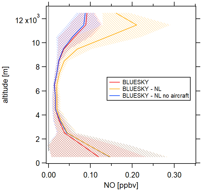
Figure 4NO vertical profiles for BLUESKY (red), for the BLUESKY no-lockdown scenario (yellow) and for the BLUESKY no-lockdown scenario without aircraft emissions (blue) (model data). Upper-tropospheric NO reductions observed for BLUESKY can be attributed to reduced air traffic during the COVID-19 lockdowns.
Figure 3b presents the O3 vertical profiles. For all campaigns, O3 mixing ratios were lowest at ground level, with values of around 50 ppbv, and increased with increasing altitude up to around 140 ppbv above 10 km altitude. No significant differences between the campaigns can be observed. While ozone concentrations are dependent on various effects such as precursor levels (including NOx and VOCs) or meteorology, seasonal variations with a maximum around summertime and a minimum during winter months are also of importance (Logan, 1985). The campaigns shown here include different seasons: the HOOVER campaigns took place in October and July, and the UTOPIHAN campaigns include data from July and March. Figure S6 shows the vertical profiles of ozone separated into different seasons, for both modeled and measured data. Comparing late spring/early summer data of the three field campaigns reveals that O3 levels during BLUESKY were lower compared to HOOVER and UTOPIHAN, which is in line with findings from Clark et al. (2021), Chang et al. (2022), Bouarar et al. (2021) and Miyazaki et al. (2021).
CO vertical profiles can be seen in Fig. 3c. Ground-level mixing ratios were 181.4 ± 39.4 ppbv for UTOPIHAN, 146.4 ± 63.2 ppbv for HOOVER and slightly lower with 103.2 ± 9.2 ppbv for BLUESKY. Mixing ratios slightly decreased with altitude. Above 3 km altitude, CO for HOOVER was lower compared to the other campaigns (mostly between 70 and 80 ppbv). Mixing ratios for UTOPIHAN were slightly higher up to 11 km altitude (between 90 and 110 ppbv) compared to BLUESKY (between 80 and 100 ppbv), but generally, significant differences are not evident.
Figure 3d shows the vertical profiles of NO2 mixing ratios. Similar to NO, ground-level NO2 mixing ratios were highest for UTOPIHAN and HOOVER, with 1.57 ± 0.77 ppbv and 2.58 ± 2.72 ppbv, respectively. In contrast, mixing ratios for BLUESKY were 0.39 ± 0.30 ppbv and 0.49 ± 0.38 ppbv considering the no-lockdown scenario, which yields a 20 % NO2 lockdown reduction, as observed for NO. We show the NO2 range 0–1 ppbv for enabling the campaign distinction at low mixing ratios and present the full range in Fig. S7. As expected for NO2, mixing ratios decreased with increasing altitude. No differences between the campaigns can be observed for mid-range altitudes. In the upper troposphere, NO2 mixing ratios for the individual campaigns showed the same behavior as for NO. Above 10 km altitude, NO2 was on average 100.6 ± 93.2 pptv for UTOPIHAN, 70.5± 13.5 pptv for HOOVER and 43.1 ± 23.1 pptv for the no-lockdown scenario for BLUESKY. In comparison, BLUESKY NO2 mixing ratios were 19.9 ± 9.8 pptv, which corresponds to a 55 % reduction. In contrast to NO, NO2 reductions were relatively higher in the upper troposphere but absolutely higher at the surface.
Figure 3e and f show the vertical profiles of HOx. HO2 mixing ratios were highest at mid-range altitudes (2–6 km), with values up to 20 pptv, and decreased aloft. OH mixing ratios were lowest at the surface (0.1–0.2 pptv) and increased with altitude. Above 10 km altitude, OH mixing ratios were 0.62 ± 0.38 pptv for UTOPIHAN, 0.40 ± 0.24 pptv for HOOVER, 0.30 ± 0.06 pptv for BLUESKY and 0.39 ± 0.08 pptv for the no-lockdown scenario.
3.2.2 Net ozone production rates

Figure 5Vertical profiles of (a) net ozone production rates, (b) O3 production via NO2 photolysis, (c) O3 loss via reaction with NO, (d) O3 loss via photolysis, (e) O3 loss via reaction with HO2 and (f) O3 loss via reaction with OH for the campaigns UTOPIHAN (green), HOOVER (blue) and BLUESKY (red) and the no-lockdown (NL) scenario (yellow). The number of data points averaged per altitude bin are displayed in Table S2.
Figure 5 shows the vertical profiles of O3 production and loss terms. All calculations were performed using model data (justified by the findings from Sect. 3.1) as a full set of in situ observations is only available for HOOVER, but not for UTOPIHAN and BLUESKY. Figure 5a presents net ozone production rates, which were highest at the surface, with values between 1 and 2 ppbv h−1, but had large atmospheric variabilities, represented by the 1σ variability shades from the vertical bin averaging. NOPRs then decreased with increasing altitude. For the HOOVER campaigns, O3 loss dominated between 3 and 6 km altitude, with NOPRs of pptv h−1. Negative NOPRs were also found for BLUESKY between 4 and 7 km, with pptv h−1, and for UTOPIHAN as well as the no-lockdown BLUESKY scenario between 5 and 6 km. NOPRs were mostly positive and constant aloft. Above 10 km altitude, NOPRs were 91.7 ± 260.9 pptv h−1 for UTOPIHAN (51 data points), 71.2 ± 151.5 pptv h−1 for HOOVER (25 data points), 60.7 ± 39.7 pptv h−1 for BLUESKY (130 data points) and 61.4 ± 99.8 pptv h−1 for the no-lockdown scenario. The error ranges are large and overlapping, and therefore significant differences between the campaigns cannot be observed.
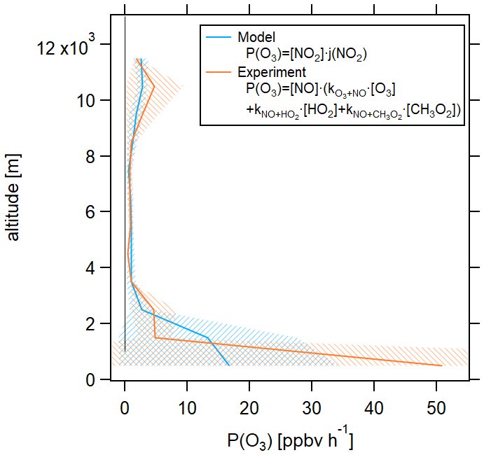
Figure 6Modeled and experimental vertical profiles of P(O3) for HOOVER. Modeled P(O3) was calculated via NO2 photolysis, and experimental P(O3) was calculated via the extended Leighton ratio as shown in Eq. (2).
Figure 5b shows O3 production. We calculated the P(O3) via the photolysis of NO2. In contrast, NO2 is not available experimentally for the HOOVER campaign, in which case the approximation via the extended Leighton ratio as shown in Eq. (2) is necessary. Modeled P(O3) via NO2 photolysis and measured P(O3) via reaction of NO with O3, OH and HO2 are in good agreement, which we show in Fig. 6. The only relevant deviation is observed at ground level, where the experimental value is significantly higher compared to the modeled value. However, only three data points were available for the calculation, with a 1σ standard deviation of the averaging of >100 %. Similar to NOPRs in Fig. 5a, ground-level P(O3) shows large variability, with absolute values of around 10 ppbv h−1 for BLUESKY and values of around 20 ppbv h−1 for UTOPIHAN and HOOVER. The production term then decreased with altitude for each campaign. Significant differences between the campaigns can only be observed at high altitudes. Above 10 km, P(O3) was 4.55 ± 3.82 ppbv h−1 for UTOPIHAN (51 data points) and 2.68 ± 0.90 ppbv h−1 for HOOVER (25 data points). For BLUESKY with the no-lockdown scenario, P(O3) was 2.17 ± 0.95 ppbv h−1 (130 data points), and in comparison, lockdown values were on average 0.97 ± 0.41 ppbv h−1, which corresponds to a 55 % reduction in ozone production. We observed the same relative reduction as for NO and NO2 mixing ratios.
Figure 5c presents the vertical profiles of O3 loss via the reaction with NO, which show a similar course compared to the P(O3) profiles. Above 10 km, O3 loss via reaction with NO was largest for UTOPIAN, with 4.37 ± 3.82 ppbv h−1, followed by HOOVER, with 2.56 ± 0.87 ppbv h−1. For BLUESKY, a loss of 0.86 ± 0.42 ppbv h−1 was observed during the lockdown and a loss of 2.05 ± 1.02 ppbv h−1 for the no-lockdown scenario. Figure 5d–f present additional considered loss pathways for O3 via photolysis and via the reactions with HO2 and OH. It can be seen that these O3 losses are negligibly small in comparison to the loss via NO, and no significant differences between the campaigns were present.
Consequently, net production of ozone was dominated by NOx chemistry for all campaigns, and variations in production and loss terms corresponded to the mixing ratios of NO and NO2 as presented in Fig. 3. In the campaign comparison, higher NOx concentrations (as for example for UTOPIHAN) lead to higher production and loss terms of O3 and vice versa. For the BLUESKY campaign, this analysis shows that the lockdown did not affect net ozone production rates but instead impacted the cycling of O3 such that both production and loss rates were decreased through the reduced availability of NO and NO2 in the upper troposphere.
3.3 Chemical regime

Figure 7 for the campaigns UTOPIHAN (green), HOOVER (blue) and BLUESKY (red) and the no-lockdown (NL) scenario (yellow) (a) as a vertical profile, (b) in correlation with NO below 2 km and (c) in correlation with NO above 10 km.
As described above, the share of methyl peroxyradicals forming formaldehyde can be a measure for the dominant chemical regime when correlated with NO mixing ratios. We have previously validated this method in a comparison to the established method of analyzing the HCHONO2 ratio (Nussbaumer et al., 2021). HCHO can be formed by almost any hydrocarbon and is therefore a proxy for VOCs, which are often not measured in their entirety. Likewise, – representing the HCHO yield from methyl peroxy radicals – is capable of revealing the dominant chemical regime without the knowledge of ambient VOC levels. Figure 7a shows the vertical profiles of for all available data points for all campaigns based on the model simulation. values were close to 1 at the surface and decreased with altitude up to around 5 km, where values of around 0.6 were observed, with no significant differences between the campaigns. increased again aloft, whereas it was lowest for the BLUESKY campaign. Above 10 km, was 0.97 ± 0.03 for UTOPIHAN, 0.98 ± 0.01 for HOOVER and 0.96 ± 0.04 for the no-lockdown scenario for BLUESKY. In comparison, was lower for BLUESKY, with 0.90 ± 0.06.
Figure 7b and c present in correlation with NO mixing ratios below 2 km altitude and above 10 km altitude, respectively, based on model results. Below 2 km altitude, ranged between 0.5 and 1.0 over the NO range of 0–1 ppbv. No significant trends or differences can be observed. We show between 2 and 10 km altitude in Fig. S8, which does not present any differences between the campaigns either. In contrast, above 10 km altitude, tropospheric showed a different behavior for each campaign. For an easier distinction, we show each campaign in an individual panel in Fig. S9. For UTOPIHAN, was high and almost non-responsive to changing NO mixing ratios, with a slope of NO ppbv−1. In contrast, for BLUESKY was between 0.75 and 1. Small changes in NO mixing ratios caused large changes in , with a slope of 1.12 ± 0.08 ppbv−1. For the no-lockdown scenario the response of to NO was intermediate between UTOPIHAN and BLUESKY with a slope of 0.37 ± 0.03 ppbv−1. These observations suggest that a VOC-limited chemical regime was present during the UTOPIHAN campaign in the upper troposphere and a transition regime during the BLUESKY no-lockdown scenario, likely due to emission control over time. For BLUESKY, we observe a distinct NOx limitation in the upper troposphere, which is related to the lockdown conditions. Aircraft NOx emissions are much larger than aircraft VOC emissions (Schumann, 2002). We can therefore expect reduced air traffic to effect lower NOVOC ratios, shifting chemistry towards a NOx-limited regime. Lamprecht et al. (2021) reported ground-level reductions in several aromatic VOCs during the COVID-19 lockdown to be comparable to NOx reductions in Europe, implicating a steady NOVOC level and therefore no changes in the dominating chemical regime, which is in line with our findings for the lower troposphere. Only few data points were available for HOOVER, which were observed at similar NO levels, and the response of to NO can therefore not be investigated. While the NOPRs did not change under lockdown conditions due to compensating effects in the NOx chemistry, we can expect impacts on tropospheric ozone from changes in VOCs (including CH4) relevant for future emission scenarios. The effects of NOx aircraft emissions on O3 and CH4 have been previously discussed for pre-lockdown conditions in Khodayari et al. (2014) and Khodayari et al. (2015), who present increased methane loss rates and a shorter lifetime as a response to increased OH concentrations from aviation as well as higher ozone production rates. Having investigated NOPRs in this study, lockdown effects on CH4 loss in the upper troposphere induced by reduced air traffic could be subject to future studies.
In this study, we present in situ observations of atmospheric trace gases and model simulations from the EMAC model for three different aircraft campaigns across Europe: the UTOPIHAN campaigns in 2003/04, the HOOVER campaigns in 2006/07 and the BLUESKY campaign in 2020, including a modeled “no-lockdown scenario” with business-as-usual emissions for the latter. We found that model results can reproduce in situ observations well and thus could be used for further analysis which benefits from a more complete set of parameters and a higher data coverage. While observations for O3, CO and HOx were very similar for all campaigns, NOx showed significant differences, particularly in the upper troposphere, where mixing ratios were highest for UTOPIHAN and HOOVER, followed by the no-lockdown scenario for BLUESKY. Observed NO and NO2 emissions during the BLUESKY campaign were approximately 55 % lower compared to the modeled no-lockdown scenario, which are attributed to reduced aircraft activity at these altitudes due to the COVID-19 travel restrictions. We found a similar trend in production and loss terms of O3, which were dominated by NOx chemistry. The COVID-19 lockdown caused a significant deceleration in O3 cycling, whereas net ozone production rates were not affected by the emission reductions. Finally, we showed that chemistry in the upper troposphere was VOC-limited during the UTOPIHAN campaign, NOx-limited during the BLUESKY campaign and in a transition regime for the BLUESKY no-lockdown scenario. While ground-level chemistry regimes were not found to be affected, the COVID-19 lockdown caused the predominant chemistry to shift from a transition regime to a clear NOx-limited regime at high altitudes.
We found that the three aircraft campaigns, performed over a period of 17 years, represent the range from VOC- to NOx-limited tropospheric ozone chemistry, which can help analyze the impacts of anthropogenic emission scenarios. We encourage future studies to investigate the dominating chemical regime in the upper troposphere, a topic which has not received much attention in the literature so far, in order to get a deeper understanding of photochemical processes and the dominant ozone chemistry in a range of the atmosphere which receives its main NOx emissions from air traffic and lightning. The COVID-19 lockdown has been a unique opportunity to examine the effect of sharp reductions in primary pollutants on our atmosphere and could be a guidepost for future air policy in an effort to decrease anthropogenic emissions and to decelerate global warming.
Data measured during the flight campaigns BLUESKY, UTOPIHAN and HOOVER are available upon request at https://keeper.mpdl.mpg.de/ (last access: 9 May 2022) to all scientists agreeing to the respective data protocols. The model results used in this study are available upon request to the author.
The supplement related to this article is available online at: https://doi.org/10.5194/acp-22-6151-2022-supplement.
CMN and HF had the idea and designed the study. CMN analyzed the data and wrote the manuscript. AP provided the modeling data. IT provided NO data for BLUESKY. CO data for BLUESKY were received from LR. O3 data for BLUESKY were obtained from FO. HH provided HOx data for HOOVER. JL and HF were significantly involved in planning and operating the research campaign.
At least one of the (co-)authors is a member of the editorial board of Atmospheric Chemistry and Physics. The peer-review process was guided by an independent editor, and the authors also have no other competing interests to declare.
Publisher’s note: Copernicus Publications remains neutral with regard to jurisdictional claims in published maps and institutional affiliations.
This article is part of the special issue “BLUESKY atmospheric composition measurements by aircraft during the COVID-19 lockdown in spring 2020”. It is not associated with a conference.
We acknowledge Simon Reifenberg for preparing the input data for EMAC. This work was supported by the Max Planck Graduate Center (MPGC) with the Johannes Gutenberg-Universität Mainz.
The article processing charges for this open-access publication were covered by the Max Planck Society.
This paper was edited by Stefania Gilardoni and reviewed by two anonymous referees.
Balamurugan, V., Chen, J., Qu, Z., Bi, X., Gensheimer, J., Shekhar, A., Bhattacharjee, S., and Keutsch, F. N.: Tropospheric NO2 and O3 response to COVID-19 lockdown restrictions at the national and urban scales in Germany, J. Geophys. Res.-Atmos., 126, 1–15, https://doi.org/10.1029/2021JD035440, 2021. a
Bouarar, I., Gaubert, B., Brasseur, G. P., Steinbrecht, W., Doumbia, T., Tilmes, S., Liu, Y., Stavrakou, T., Deroubaix, A., Darras, S., Granier, C., Lacey, F., Müller, J.-F., Shi, X., Elguindi, N., and Wang, T.: Ozone Anomalies in the Free Troposphere During the COVID-19 Pandemic, Geophys. Res. Lett., 48, e2021GL094204, https://doi.org/10.1029/2021GL094204, 2021. a, b, c
Bozem, H., Butler, T. M., Lawrence, M. G., Harder, H., Martinez, M., Kubistin, D., Lelieveld, J., and Fischer, H.: Chemical processes related to net ozone tendencies in the free troposphere, Atmos. Chem. Phys., 17, 10565–10582, https://doi.org/10.5194/acp-17-10565-2017, 2017a. a, b, c
Bozem, H., Pozzer, A., Harder, H., Martinez, M., Williams, J., Lelieveld, J., and Fischer, H.: The influence of deep convection on HCHO and H2O2 in the upper troposphere over Europe, Atmos. Chem. Phys., 17, 11835–11848, https://doi.org/10.5194/acp-17-11835-2017, 2017b. a
Brockmann Lab: Covid-19 Mobility Project, http://covid-19-mobility.org/, last access: 9 March 2022. a
Calvert, J. G. and Stockwell, W. R.: Deviations from the O3–NO–NO2 photostationary state in tropospheric chemistry, Can. J. Chem., 61, 983–992, https://doi.org/10.1139/v83-174, 1983. a
Cazorla, M., Herrera, E., Palomeque, E., and Saud, N.: What the COVID-19 lockdown revealed about photochemistry and ozone production in Quito, Ecuador, Atmos. Pollut. Res., 12, 124–133, https://doi.org/10.1016/j.apr.2020.08.028, 2021. a
Chang, K.-l., Cooper, O. R., Gaudel, A., Allaart, M., Ancellet, G., Clark, H., Godin-Beekmann, S., Leblanc, T., Van Malderen, R., Nédélec, P., Petropavlovskikh, I., Steinbrecht, W., Stübi, R., Tarasick, D. W., and Torres, C.: Impact of the COVID-19 Economic Downturn on Tropospheric Ozone Trends: An Uncertainty Weighted Data Synthesis for Quantifying Regional Anomalies Above Western North America and Europe, AGU Advances, 3, e2021AV000542, https://doi.org/10.1029/2021AV000542, 2022. a, b
Chossière, G. P., Xu, H., Dixit, Y., Isaacs, S., Eastham, S. D., Allroggen, F., Speth, R. L., and Barrett, S. R.: Air pollution impacts of COVID-19-related containment measures, Sci. Adv., 7, 1–10, https://doi.org/10.1126/sciadv.abe1178, 2021. a, b
Clark, H., Bennouna, Y., Tsivlidou, M., Wolff, P., Sauvage, B., Barret, B., Le Flochmoën, E., Blot, R., Boulanger, D., Cousin, J.-M., Nédélec, P., Petzold, A., and Thouret, V.: The effects of the COVID-19 lockdowns on the composition of the troposphere as seen by In-service Aircraft for a Global Observing System (IAGOS) at Frankfurt, Atmos. Chem. Phys., 21, 16237–16256, https://doi.org/10.5194/acp-21-16237-2021, 2021. a, b
Colomb, A., Williams, J., Crowley, J., Gros, V., Hofmann, R., Salisbury, G., Klüpfel, T., Kormann, R., Stickler, A., Forster, C., and Lelieveld, J.: Airborne measurements of trace organic species in the upper troposphere over Europe: the impact of deep convection, Environ. Chem., 3, 244–259, https://doi.org/10.1071/EN06020, 2006. a
Cristofanelli, P., Arduni, J., Serva, F., Calzolari, F., Bonasoni, P., Busetto, M., Maione, M., Sprenger, M., Trisolino, P., and Putero, D.: Negative ozone anomalies at a high mountain site in northern Italy during 2020: a possible role of COVID-19 lockdowns?, Environ. Res. Lett., 16, 074029, https://doi.org/10.1088/1748-9326/ac0b6a, 2021. a
Crutzen, P. J.: Tropospheric ozone: An overview, in: Mathematical and Physical Sciences, 1st edn., edited by: Isaksen, I. S. A., Vol. 227, Springer, 3–32, https://doi.org/10.1007/978-94-009-2913-5_1, 1988. a
Donzelli, G., Cioni, L., Cancellieri, M., Llopis-Morales, A., and Morales-Suárez-Varela, M.: Relations between air quality and COVID-19 lockdown measures in Valencia, Spain, Int. J. Env. Res. Pub. He., 18, 2296, https://doi.org/10.3390/ijerph18052296, 2021. a
Duncan, B. N., Yoshida, Y., Olson, J. R., Sillman, S., Martin, R. V., Lamsal, L., Hu, Y., Pickering, K. E., Retscher, C., Allen, D. J., and Crawford, J. H.: Application of OMI observations to a space-based indicator of NOx and VOC controls on surface ozone formation, Atmos. Environ., 44, 2213–2223, https://doi.org/10.1016/j.atmosenv.2010.03.010, 2010. a, b
EUROCONTROL: COVID-19 impact on the European air traffic network, https://www.eurocontrol.int/covid19, last access: 9 March 2022. a
Forster, P. M., Forster, H. I., Evans, M. J., Gidden, M. J., Jones, C. D., Keller, C. A., Lamboll, R. D., Le Quéré, C., Rogelj, J., Rosen, D., Schleussner , C.-F., Richardson, T. B., Smith , C. J., and Turnock, S. T.: Current and future global climate impacts resulting from COVID-19, Nat. Clim. Change, 10, 913–919, https://doi.org/10.1038/s41558-020-0883-0, 2020. a
Gaubert, B., Bouarar, I., Doumbia, T., Liu, Y., Stavrakou, T., Deroubaix, A., Darras, S., Elguindi, N., Granier, C., Lacey, F., Müller, J.-F., Shi, X., Tilmes, S., Wang, T., and Brasseur, G. P.: Global changes in secondary atmospheric pollutants during the 2020 COVID-19 pandemic, J. Geophys. Res.-Atmos., 126, 1–22, https://doi.org/10.1029/2020JD034213, 2021. a
Grange, S. K., Lee, J. D., Drysdale, W. S., Lewis, A. C., Hueglin, C., Emmenegger, L., and Carslaw, D. C.: COVID-19 lockdowns highlight a risk of increasing ozone pollution in European urban areas, Atmos. Chem. Phys., 21, 4169–4185, https://doi.org/10.5194/acp-21-4169-2021, 2021. a
Gurk, Ch., Fischer, H., Hoor, P., Lawrence, M. G., Lelieveld, J., and Wernli, H.: Airborne in-situ measurements of vertical, seasonal and latitudinal distributions of carbon dioxide over Europe, Atmos. Chem. Phys., 8, 6395–6403, https://doi.org/10.5194/acp-8-6395-2008, 2008. a
Hasegawa, T.: Effects of Novel Coronavirus (COVID‐19) on Civil Aviation: Economic Impact Analysis, https://www.icao.int/sustainability/Documents/Covid-19/ICAO_coronavirus_Econ_Impact.pdf, last access: 9 March 2022. a
Higham, J., Ramírez, C. A., Green, M., and Morse, A.: UK COVID-19 lockdown: 100 days of air pollution reduction?, Air Qual. Atmos. Health, 14, 325–332, https://doi.org/10.1007/s11869-020-00937-0, 2021. a
Hosaynali Beygi, Z., Fischer, H., Harder, H. D., Martinez, M., Sander, R., Williams, J., Brookes, D. M., Monks, P. S., and Lelieveld, J.: Oxidation photochemistry in the Southern Atlantic boundary layer: unexpected deviations of photochemical steady state, Atmos. Chem. Phys., 11, 8497–8513, https://doi.org/10.5194/acp-11-8497-2011, 2011. a, b
IUPAC Task Group on Atmospheric Chemical Kinetic Data Evaluation: Evaluated Kinetic Data, http://iupac.pole-ether.fr, last access: 3 November 2021. a, b
Jin, X., Fiore, A., Boersma, K. F., Smedt, I. D., and Valin, L.: Inferring Changes in Summertime Surface Ozone–NOx–VOC Chemistry over U.S. Urban Areas from Two Decades of Satellite and Ground-Based Observations, Environ. Sci. Technol., 54, 6518–6529, https://doi.org/10.1021/acs.est.9b07785, 2020. a
Jöckel, P., Tost, H., Pozzer, A., Kunze, M., Kirner, O., Brenninkmeijer, C. A. M., Brinkop, S., Cai, D. S., Dyroff, C., Eckstein, J., Frank, F., Garny, H., Gottschaldt, K.-D., Graf, P., Grewe, V., Kerkweg, A., Kern, B., Matthes, S., Mertens, M., Meul, S., Neumaier, M., Nützel, M., Oberländer-Hayn, S., Ruhnke, R., Runde, T., Sander, R., Scharffe, D., and Zahn, A.: Earth System Chemistry integrated Modelling (ESCiMo) with the Modular Earth Submodel System (MESSy) version 2.51, Geosci. Model Dev., 9, 1153–1200, https://doi.org/10.5194/gmd-9-1153-2016, 2016. a, b
Khodayari, A., Tilmes, S., Olsen, S. C., Phoenix, D. B., Wuebbles, D. J., Lamarque, J.-F., and Chen, C.-C.: Aviation 2006 NOx-induced effects on atmospheric ozone and HOx in Community Earth System Model (CESM), Atmos. Chem. Phys., 14, 9925–9939, https://doi.org/10.5194/acp-14-9925-2014, 2014. a
Khodayari, A., Olsen, S. C., Wuebbles, D. J., and Phoenix, D. B.: Aviation NOx-induced CH4 effect: Fixed mixing ratio boundary conditions versus flux boundary conditions, Atmos. Environ., 113, 135–139, https://doi.org/10.1016/j.atmosenv.2015.04.070, 2015. a
Kleinman, L. I., Daum, P. H., Lee, Y.-N., Nunnermacker, L. J., Springston, S. R., Weinstein-Lloyd, J., and Rudolph, J.: Sensitivity of ozone production rate to ozone precursors, Geophys. Res. Lett., 28, 2903–2906, https://doi.org/10.1029/2000GL012597, 2001. a
Klippel, T., Fischer, H., Bozem, H., Lawrence, M. G., Butler, T., Jöckel, P., Tost, H., Martinez, M., Harder, H., Regelin, E., Sander, R., Schiller, C. L., Stickler, A., and Lelieveld, J.: Distribution of hydrogen peroxide and formaldehyde over Central Europe during the HOOVER project, Atmos. Chem. Phys., 11, 4391–4410, https://doi.org/10.5194/acp-11-4391-2011, 2011. a, b
Kormann, R., Königstedt, R., Parchatka, U., Lelieveld, J., and Fischer, H.: QUALITAS: A mid-infrared spectrometer for sensitive trace gas measurements based on quantum cascade lasers in CW operation, Rev. Sci. Instrum., 76, 075102, https://doi.org/10.1063/1.1931233, 2005. a
Kroll, J. H., Heald, C. L., Cappa, C. D., Farmer, D. K., Fry, J. L., Murphy, J. G., and Steiner, A. L.: The complex chemical effects of COVID-19 shutdowns on air quality, Nat. Chem., 12, 777–779, https://doi.org/10.1038/s41557-020-0535-z, 2020. a, b
Lamprecht, C., Graus, M., Striednig, M., Stichaner, M., and Karl, T.: Decoupling of urban CO2 and air pollutant emission reductions during the European SARS-CoV-2 lockdown, Atmos. Chem. Phys., 21, 3091–3102, https://doi.org/10.5194/acp-21-3091-2021, 2021. a
Lee, D. S., Fahey, D., Skowron, A., Allen, M., Burkhardt, U., Chen, Q., Doherty, S., Freeman, S., Forster, P., Fuglestvedt, J., Gettelman, A., Leon, R. D., Lim, L., Lund, M., Millar, R., Owen, B., Penner, J., Pitari, G., Prather, M., Sausen, R., and Wilcox, L.: The contribution of global aviation to anthropogenic climate forcing for 2000 to 2018, Atmos. Environ., 244, 117834, https://doi.org/10.1016/j.atmosenv.2020.117834, 2021. a
Leighton, P. A.: Photochemistry of air pollution, Academic Press Inc., 2nd edn., New York, ISBN 9780323156455, 1971. a, b
Lelieveld, J. and Dentener, F. J.: What controls tropospheric ozone?, J. Geophys. Res.-Atmos., 105, 3531–3551, https://doi.org/10.1029/1999JD901011, 2000. a
LI-COR, Inc.: LI-6262 CO2/H2O Analyzer Operating and Service Manual, https://www.licor.com/documents/umazybbyhzalz840pf63a1137qz7ofib (last access: 6 December 2021), 1996. a
Lin, X., Trainer, M., and Liu, S.: On the nonlinearity of the tropospheric ozone production, J. Geophys. Res.-Atmos., 93, 15879–15888, https://doi.org/10.1029/JD093iD12p15879, 1988. a
Liu, S., Trainer, M., Fehsenfeld, F., Parrish, D., Williams, E., Fahey, D. W., Hübler, G., and Murphy, P. C.: Ozone production in the rural troposphere and the implications for regional and global ozone distributions, J. Geophys. Res.-Atmos., 92, 4191–4207, https://doi.org/10.1029/JD092iD04p04191, 1987. a
Logan, J. A.: Tropospheric ozone: Seasonal behavior, trends, and anthropogenic influence, J. Geophys. Res.-Atmos., 90, 10463–10482, https://doi.org/10.1029/JD090iD06p10463, 1985. a, b
Matthias, V., Quante, M., Arndt, J. A., Badeke, R., Fink, L., Petrik, R., Feldner, J., Schwarzkopf, D., Link, E.-M., Ramacher, M. O. P., and Wedemann, R.: The role of emission reductions and the meteorological situation for air quality improvements during the COVID-19 lockdown period in central Europe, Atmos. Chem. Phys., 21, 13931–13971, https://doi.org/10.5194/acp-21-13931-2021, 2021. a, b
Menut, L., Bessagnet, B., Siour, G., Mailler, S., Pennel, R., and Cholakian, A.: Impact of lockdown measures to combat Covid-19 on air quality over western Europe, Sci. Total Environ., 741, 140426, https://doi.org/10.1016/j.scitotenv.2020.140426, 2020. a
Mertens, M., Jöckel, P., Matthes, S., Nützel, M., Grewe, V., and Sausen, R.: COVID-19 induced lower-tropospheric ozone changes, Environ. Res. Lett., 16, 1–9, https://doi.org/10.1088/1748-9326/abf191, 2021. a
Mills, G., Pleijel, H., Malley, C. S., Sinha, B., Cooper, O. R., Schultz, M. G., Neufeld, H. S., Simpson, D., Sharps, K., Feng, Z., Gerosa, G., Harmens, H., Kobayashi, K., Saxena, P., Paoletti, E., Sinha, V., and Xu, X.: Tropospheric Ozone Assessment Report: Present-day tropospheric ozone distribution and trends relevant to vegetation, Elementa, 6, 47, https://doi.org/10.1525/elementa.302, 2018. a
Miyazaki, K., Bowman, K., Sekiya, T., Takigawa, M., Neu, J. L., Sudo, K., Osterman, G., and Eskes, H.: Global tropospheric ozone responses to reduced NOx emissions linked to the COVID-19 worldwide lockdowns, Sci. Adv., 7, 1–14, https://doi.org/10.1126/sciadv.abf7460, 2021. a
National Research Council – Committee on Tropospheric Ozone: Rethinking the ozone problem in urban and regional air pollution, 1st edn., National Academy Press, Washington D.C., https://doi.org/10.17226/1889, 1992. a
Nussbaumer, C. M. and Cohen, R. C.: The Role of Temperature and NOx in Ozone Trends in the Los Angeles Basin, Environ. Sci. Technol., 54, 15652–15659, https://doi.org/10.1021/acs.est.0c04910, 2020. a, b
Nussbaumer, C. M., Crowley, J. N., Schuladen, J., Williams, J., Hafermann, S., Reiffs, A., Axinte, R., Harder, H., Ernest, C., Novelli, A., Sala, K., Martinez, M., Mallik, C., Tomsche, L., Plass-Dülmer, C., Bohn, B., Lelieveld, J., and Fischer, H.: Measurement report: Photochemical production and loss rates of formaldehyde and ozone across Europe, Atmos. Chem. Phys., 21, 18413–18432, https://doi.org/10.5194/acp-21-18413-2021, 2021. a, b, c, d
Nuvolone, D., Petri, D., and Voller, F.: The effects of ozone on human health, Environ. Sci. Pollut. Res., 25, 8074–8088, https://doi.org/10.1007/s11356-017-9239-3, 2018. a
Onyeaka, H., Anumudu, C. K., Al-Sharify, Z. T., Egele-Godswill, E., and Mbaegbu, P.: COVID-19 pandemic: A review of the global lockdown and its far-reaching effects, Sci. Prog., 104, 1–18, https://doi.org/10.1177/00368504211019854, 2021. a
Ordóñez, C., Garrido-Perez, J. M., and García-Herrera, R.: Early spring near-surface ozone in Europe during the COVID-19 shutdown: Meteorological effects outweigh emission changes, Sci. Total Environ., 747, 14322, https://doi.org/10.1016/j.scitotenv.2020.141322, 2020. a
Parrish, D., Lamarque, J.-F., Naik, V., Horowitz, L., Shindell, D., Staehelin, J., Derwent, R., Cooper, O., Tanimoto, H., Volz-Thomas, A., Gilge, S., Scheel, H.-E., Steinbacher, M., and Fröhlich, M.: Long-term changes in lower tropospheric baseline ozone concentrations: Comparing chemistry-climate models and observations at northern midlatitudes, J. Geophys. Res.-Atmos., 119, 5719–5736, https://doi.org/10.1002/2013JD021435, 2014. a
Pusede, S. and Cohen, R.: On the observed response of ozone to NOx and VOC reactivity reductions in San Joaquin Valley California 1995–present, Atmos. Chem. Phys., 12, 8323–8339, https://doi.org/10.5194/acp-12-8323-2012, 2012. a, b, c
Pusede, S. E., Steiner, A. L., and Cohen, R. C.: Temperature and recent trends in the chemistry of continental surface ozone, Chem. Rev., 115, 3898–3918, https://doi.org/10.1021/cr5006815, 2015. a, b
Regelin, E., Harder, H., Martinez, M., Kubistin, D., Tatum Ernest, C., Bozem, H., Klippel, T., Hosaynali-Beygi, Z., Fischer, H., Sander, R., Jöckel, P., Königstedt, R., and Lelieveld, J.: HOx measurements in the summertime upper troposphere over Europe: a comparison of observations to a box model and a 3-D model, Atmos. Chem. Phys., 13, 10703–10720, https://doi.org/10.5194/acp-13-10703-2013, 2013. a, b
Reifenberg, S. F., Martin, A., Kohl, M., Hamryszczak, Z., Tadic, I., Röder, L., Crowley, D., Fischer, H., Kaiser, K., Schneider, J., Dörich, R., Crowley, J. N., Tomsche, L., Marsing, A., Voigt, C., Zahn, A., Pöhlker, C., Hollanda, B., Krüger, O., Pöschl, U., Pöhlker, M., Lelieveld, J., and Pozzer, A.: Impact of reduced emissions on direct and indirect aerosol radiative forcing during COVID-19 lockdown in Europe, in preparation, 2022. a, b, c
Revell, L. E., Stenke, A., Tummon, F., Feinberg, A., Rozanov, E., Peter, T., Abraham, N. L., Akiyoshi, H., Archibald, A. T., Butchart, N., Deushi, M., Jöckel, P., Kinnison, D., Michou, M., Morgenstern, O., O'Connor, F. M., Oman, L. D., Pitari, G., Plummer, D. A., Schofield, R., Stone, K., Tilmes, S., Visioni, D., Yamashita, Y., and Zeng, G.: Tropospheric ozone in CCMI models and Gaussian process emulation to understand biases in the SOCOLv3 chemistry–climate model, Atmos. Chem. Phys., 18, 16155–16172, https://doi.org/10.5194/acp-18-16155-2018, 2018. a
Rosanka, S., Sander, R., Franco, B., Wespes, C., Wahner, A., and Taraborrelli, D.: Oxidation of low-molecular-weight organic compounds in cloud droplets: global impact on tropospheric oxidants, Atmos. Chem. Phys., 21, 9909–9930, https://doi.org/10.5194/acp-21-9909-2021, 2021. a
Salma, I., Vörösmarty, M., Gyöngyösi, A. Z., Thén, W., and Weidinger, T.: What can we learn about urban air quality with regard to the first outbreak of the COVID-19 pandemic? A case study from central Europe, Atmos. Chem. Phys., 20, 15725–15742, https://doi.org/10.5194/acp-20-15725-2020, 2020. a
Schiller, C., Bozem, H., Gurk, C., Parchatka, U., Königstedt, R., Harris, G., Lelieveld, J., and Fischer, H.: Applications of quantum cascade lasers for sensitive trace gas measurements of CO, CH4, N2O and HCHO, Appl. Phys. B, 92, 419–430, https://doi.org/10.1007/s00340-008-3125-0, 2008. a, b
Schlosser, F., Maier, B. F., Jack, O., Hinrichs, D., Zachariae, A., and Brockmann, D.: COVID-19 lockdown induces disease-mitigating structural changes in mobility networks, P. Natl. Acad. Sci. USA, 117, 32883–32890, https://doi.org/10.1073/pnas.2012326117, 2020. a
Schumann, U.: Aircraft emissions, in: Encyclopedia of global environmental change, 3, edited by: Ian Douglas, John Wiley & Sons Ltd, Chichester, 178–186, ISBN 0471977969, 2002. a
Sillman, S., Logan, J. A., and Wofsy, S. C.: The sensitivity of ozone to nitrogen oxides and hydrocarbons in regional ozone episodes, J. Geophys. Res.-Atmos., 95, 1837–1851, https://doi.org/10.1029/JD095iD02p01837, 1990. a
Steinbrecht, W., Kubistin, D., Plass-Dülmer, C., Davies, J., Tarasick, D. W., Gathen, P. v. d., Deckelmann, H., Jepsen, N., Kivi, R., Lyall, N., Palm, M., Notholt, J., Kois, B., Oelsner, P., Allaart, M., Piters, A., Gill, M., Malderen, R. V., Delcloo, A. W., Sussmann, R., Mahieu, E., Servais, C., Romanens, G., Stübi, R., Ancellet, G., Godin-Beekmann, S., Yamanouchi, S., Strong, K., Johnson, B., Cullis, P., Petropavlovskikh, I., Hannigan2, J. W., Hernandez, J.-L., Rodriguez, A. D., Nakano, T., Chouza, F., Leblanc, T., Torres, C., Garcia, O., Röhling, A. N., Schneider, M., Blumenstock, T., Tully, M., Paton-Walsh, C., Jones, N., Querel, R., Strahan, S., Stauffer, R. M., Thompson, A. M., Inness, A., Engelen, R., Chang, K.-L., and Cooper, O. R.: COVID-19 crisis reduces free tropospheric ozone across the Northern Hemisphere, Geophys. Res. Lett., 48, 1–11, https://doi.org/10.1029/2020GL091987, 2021. a
Stickler, A., Fischer, H., Williams, J., De Reus, M., Sander, R., Lawrence, M., Crowley, J., and Lelieveld, J.: Influence of summertime deep convection on formaldehyde in the middle and upper troposphere over Europe, J. Geophys. Res.-Atmos., 111, 1–17, https://doi.org/10.1029/2005JD007001, 2006. a
Tadic, I., Crowley, J. N., Dienhart, D., Eger, P., Harder, H., Hottmann, B., Martinez, M., Parchatka, U., Paris, J.-D., Pozzer, A., Rohloff, R., Schuladen, J., Shenolikar, J., Tauer, S., Lelieveld, J., and Fischer, H.: Net ozone production and its relationship to nitrogen oxides and volatile organic compounds in the marine boundary layer around the Arabian Peninsula, Atmos. Chem. Phys., 20, 6769–6787, https://doi.org/10.5194/acp-20-6769-2020, 2020. a, b
Venter, Z. S., Aunan, K., Chowdhury, S., and Lelieveld, J.: COVID-19 lockdowns cause global air pollution declines, P. Natl. Acad. Sci. USA, 117, 18984–18990, https://doi.org/10.1073/pnas.2006853117, 2020. a
Voigt, C., Lelieveld, J., Schlager, H., Schneider, J., Curtius, J., Meerkötter, R., Sauer, D., Bugliaro, L., Bohn, B., Crowley, J. N., Erbertseder, T., Groß, S., Li, Q., Mertens, M., Pöhlker, M., Pozzer, A., Schumann, U., Tomsche, L., Williams, J., Zahn, A., Andreae, M., Borrmann, S., Bräuer, T., Dörich, R., Dörnbrack, A., Edtbauer, A., Ernle, L., Fischer, H., Giez, A., Granzin, M., Grewe, V., Hahn, V., Harder, H., Heinritzi, M., Holanda, B., Jöckel, P., Kaiser, K., Krüger, O., Lucke, J., Marsing, A., Martin, A., Matthes, S., Pöhlker, C., Pöschl, U., Reifenberg, S., Ringsdorf, A., Scheibe, M., Tadic, I., Zauner-Wieczorek, M., Henke, R., and Rapp, M.: BLUESKY aircraft mission reveals reduction in atmospheric pollution during the 2020 Corona lockdown, B. Am. Meteorol. Soc., in review, 2022. a
Wang, P., Chen, Y., Hu, J., Zhang, H., and Ying, Q.: Attribution of tropospheric ozone to NOx and VOC emissions: considering ozone formation in the transition regime, Environ. Sci. Technol., 53, 1404–1412, https://doi.org/10.1021/acs.est.8b05981, 2018. a
WHO: WHO Director-General's opening remarks at the media briefing on COVID-19 – 11 March 2020, https://www.who.int/director-general/speeches (last access: 2 November 2021), 2020a. a
WHO: Coronavirus disease 2019 (COVID-19) Situation Report – 51, https://www.who.int/docs/default-source/coronaviruse/situation-reports/20200311-sitrep-51-covid-19.pdf?sfvrsn=1ba62e57_10 (last access: 2 November 2021), 2020b. a
WHO: Coronavirus disease 2019 (COVID-19), https://www.who.int/health-topics/coronavirus#tab=tab_1, last access: 2 November 2021. a
World Meteorological Organization: WMO Air Quality and Climate Bulletin – No. 1, September 2021, edited by: Cooper, O. R., Sokhi, R. S., Nicely, J. M., Carmichael, G., Darmenov, A., Laj, P., and Liggio, J., https://library.wmo.int/index.php?lvl=notice_display&id=21942#.YTIzN9 (last access: 18 March 2022), 2021. a
Young, P. J., Naik, V., Fiore, A. M., Gaudel, A., Guo, J., Lin, M., Neu, J., Parrish, D., Rieder, H., Schnell, J., et al.: Tropospheric Ozone Assessment Report: Assessment of global-scale model performance for global and regional ozone distributions, variability, and trends, Elementa, 6, 10, https://doi.org/10.1525/elementa.265, 2018. a
Zahn, A., Weppner, J., Widmann, H., Schlote-Holubek, K., Burger, B., Kühner, T., and Franke, H.: A fast and precise chemiluminescence ozone detector for eddy flux and airborne application, Atmos. Meas. Tech., 5, 363–375, https://doi.org/10.5194/amt-5-363-2012, 2012. a
Zhu, S., Poetzscher, J., Shen, J., Wang, S., Wang, P., and Zhang, H.: Comprehensive insights into O3 changes during the COVID-19 from O3 formation regime and atmospheric oxidation capacity, Geophys. Res. Lett., 48, 1–11, https://doi.org/10.1029/2021GL093668, 2021. a