the Creative Commons Attribution 4.0 License.
the Creative Commons Attribution 4.0 License.
 | 04 May 2022
Model evaluation of short-lived climate forcers for the Arctic Monitoring and Assessment Programme: a multi-species, multi-model study
Cynthia H. Whaley
Rashed Mahmood
Knut von Salzen
Barbara Winter
Sabine Eckhardt
Stephen Arnold
Stephen Beagley
Silvia Becagli
Rong-You Chien
Jesper Christensen
Sujay Manish Damani
Xinyi Dong
Konstantinos Eleftheriadis
Nikolaos Evangeliou
Gregory Faluvegi
Mark Flanner
Joshua S. Fu
Michael Gauss
Fabio Giardi
Wanmin Gong
Jens Liengaard Hjorth
Lin Huang
Yugo Kanaya
Srinath Krishnan
Zbigniew Klimont
Thomas Kühn
Joakim Langner
Kathy S. Law
Louis Marelle
Andreas Massling
Dirk Olivié
Tatsuo Onishi
Naga Oshima
Yiran Peng
David A. Plummer
Olga Popovicheva
Luca Pozzoli
Jean-Christophe Raut
Maria Sand
Laura N. Saunders
Julia Schmale
Sangeeta Sharma
Ragnhild Bieltvedt Skeie
Henrik Skov
Fumikazu Taketani
Manu A. Thomas
Rita Traversi
Kostas Tsigaridis
Svetlana Tsyro
Steven Turnock
Vito Vitale
Kaley A. Walker
Minqi Wang
Duncan Watson-Parris
Tahya Weiss-Gibbons
While carbon dioxide is the main cause for global warming, modeling short-lived climate forcers (SLCFs) such as methane, ozone, and particles in the Arctic allows us to simulate near-term climate and health impacts for a sensitive, pristine region that is warming at 3 times the global rate. Atmospheric modeling is critical for understanding the long-range transport of pollutants to the Arctic, as well as the abundance and distribution of SLCFs throughout the Arctic atmosphere. Modeling is also used as a tool to determine SLCF impacts on climate and health in the present and in future emissions scenarios.
In this study, we evaluate 18 state-of-the-art atmospheric and Earth system models by assessing their representation of Arctic and Northern Hemisphere atmospheric SLCF distributions, considering a wide range of different chemical species (methane, tropospheric ozone and its precursors, black carbon, sulfate, organic aerosol, and particulate matter) and multiple observational datasets. Model simulations over 4 years (2008–2009 and 2014–2015) conducted for the 2022 Arctic Monitoring and Assessment Programme (AMAP) SLCF assessment report are thoroughly evaluated against satellite, ground, ship, and aircraft-based observations. The annual means, seasonal cycles, and 3-D distributions of SLCFs were evaluated using several metrics, such as absolute and percent model biases and correlation coefficients. The results show a large range in model performance, with no one particular model or model type performing well for all regions and all SLCF species. The multi-model mean (mmm) was able to represent the general features of SLCFs in the Arctic and had the best overall performance. For the SLCFs with the greatest radiative impact (CH4, O3, BC, and SO), the mmm was within ±25 % of the measurements across the Northern Hemisphere. Therefore, we recommend a multi-model ensemble be used for simulating climate and health impacts of SLCFs.
Of the SLCFs in our study, model biases were smallest for CH4 and greatest for OA. For most SLCFs, model biases skewed from positive to negative with increasing latitude. Our analysis suggests that vertical mixing, long-range transport, deposition, and wildfires remain highly uncertain processes. These processes need better representation within atmospheric models to improve their simulation of SLCFs in the Arctic environment. As model development proceeds in these areas, we highly recommend that the vertical and 3-D distribution of SLCFs be evaluated, as that information is critical to improving the uncertain processes in models.
- Article
(19748 KB) - Full-text XML
-
Supplement
(1745 KB) - BibTeX
- EndNote


The Arctic atmosphere is warming 3 times more quickly than the global average (Bush and Lemmen, 2019; NOAA, 2020; AMAP, 2021; IPCC, 2021). Arctic warming is a manifestation of global warming, and the main driver for this is the increasing carbon dioxide (CO2) radiative forcing (IPCC, 2021). Arctic warming is amplified by sea ice and snow feedbacks and affected by local radiative forcings in the Arctic, including radiative forcings by short-lived climate forcers (SLCFs), such as methane, black carbon, and tropospheric ozone (AMAP, 2015a, b, 2022). The remote pristine Arctic environment is sensitive to the long-range transport of atmospheric pollutants and deposition (Schmale et al., 2021). At the same time, it is difficult to carry out in situ measurements (Nguyen et al., 2016; Freud et al., 2017) and satellite observations over the Arctic. The majority of the Arctic surface is ocean covered with sea ice that is usually adrift for most of the year. The Arctic environment is also harsh. These aspects have historically kept surface-based measurements sparse. The overwhelming majority of the satellite observations either depend on the visible spectrum, are limited by the presence of clouds, or have very low sensitivity in the lower troposphere where the atmospheric processes mainly determine the fate of the pollutants. Many satellite measurements also do not have good coverage in the Arctic, given their orbital parameters or problems measuring areas with high albedo (Beer, 2006).
Modeling the Arctic atmosphere comes with its own challenges due to extreme meteorological conditions, its great distance from major global pollution sources, poorly known local emissions, high gradients in physical and chemical fields, and a singularity in some model grids at the pole. Models have been improving in the last 2 decades, but many models still have inaccurate results in the Arctic (Shindell et al., 2008; Eckhardt et al., 2015; Emmons et al., 2015; Sand et al., 2017; Marelle et al., 2018). That said, there has recently been a number of improvements in numerous models that have allowed for better representation of certain processes (Morgenstern et al., 2017; Emmons et al., 2020a; Swart et al., 2019; Holopainen et al., 2020; Im et al., 2021). In this study, model simulations for the 2021 Arctic Monitoring and Assessment Programme (AMAP) SLCF assessment report (AMAP, 2022) have been thoroughly evaluated by comparison to several freely available observational datasets in the Northern Hemisphere and assessed in more detail in the Arctic. In order to support the integrated assessment of climate and human health for AMAP, 6 SLCF species (methane – CH4, ozone – O3, black carbon – BC, sulfate – SO, organic aerosol – OA, and fine particulate matter – PM2.5) and 2 O3 precursors (carbon monoxide – CO; nitrogen dioxide – NO2) from 18 atmospheric or Earth system models are compared to numerous observational datasets (from three satellite instruments, seven monitoring networks, and nine measurement campaigns) for 4 years (2008–2009 and 2014–2015), with the goal of answering the following questions.
- 1.
How well do the AMAP SLCF models perform in the context of measurements and their associated uncertainty?
-
What do the best-performing models have in common?
-
Are there regional patterns in the model biases?
-
Are there patterns in the model biases between SLCF species?
- 2.
How does the model performance impact model applications, such as simulated climate and health impacts?
- 3.
What processes should be improved or studied further for better model performance?
Out of scope of this study are any sensitivity tests by the models to assess different components of model errors. Also out of scope are the models' simulations of aerosol optical properties and cloud properties (e.g., cloud fraction, cloud droplet number concentration, cloud scavenging), though those parameters do have a large impact on climate and a tight relationship with some SLCFs. Their initial evaluation can be found in AMAP (2022) (chap. 7). Estimates of effective radiative forcings of SLCFs in the Arctic by the AMAP participating models are also provided elsewhere (Oshima et al., 2020).
The next section summarizes the models used in this study, with more information in the Appendix. Section 3 summarizes the measurements used for model evaluation. Section 4 presents our model evaluation for each SLCF species, followed by a summary of all SLCFs. Finally, Sect. 5 is the conclusion where the questions posed above are answered.
In this section we briefly describe the models used for the AMAP SLCF study and refer the reader to Appendix A for individual model descriptions and further information. All models were run globally with the same anthropogenic emissions dataset (see Sect. 2.1), and most were run for the years 2008–2009 (as was done for the 2015 AMAP assessment report) and 2014–2015 (to evaluate more recent model results) inclusive for this evaluation, as these were years with numerous Arctic measurements. Unless otherwise indicated, all model output was monthly-averaged.
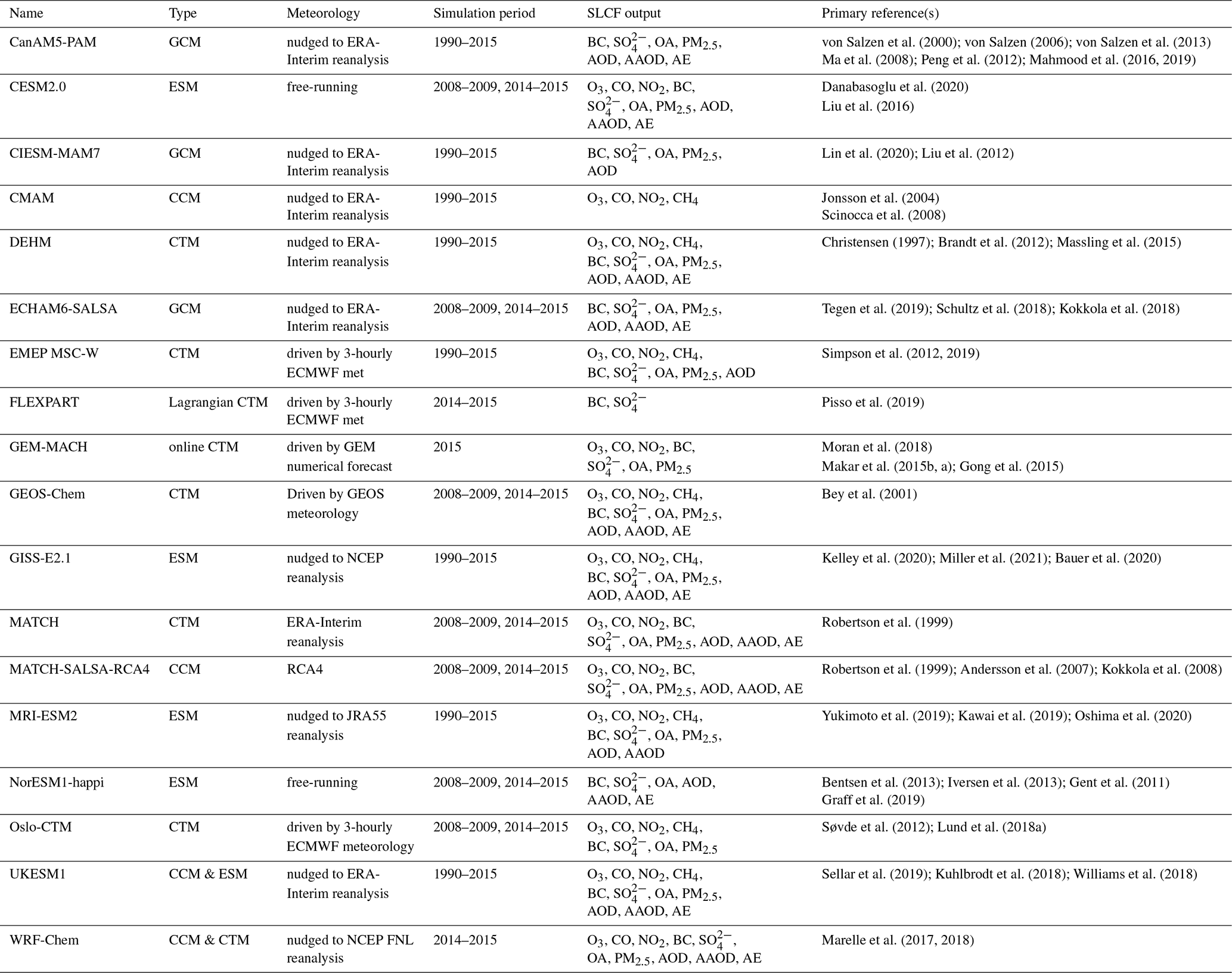
The models used for this study are summarized in Table 1. As is shown in the table, not all models provided all SLCF species, and not all models provided all 4 years. There were eight chemical transport models (CTMs), two chemistry–climate models (CCMs), three global climate models (GCMs), and five Earth system models (ESMs). Many models used specified or nudged meteorology, which allows the day-to-day variability of the model meteorology to be more closely aligned with the historical evolution of the atmosphere than occurs in a free-running model. The ERA-Interim reanalysis was the most commonly used meteorology (in 7 out of 18 models), but some were free-running (simulating their own meteorology) and some used other reanalysis products (Table 1).
von Salzen et al. (2000); von Salzen (2006); von Salzen et al. (2013)Ma et al. (2008); Peng et al. (2012); Mahmood et al. (2016, 2019)Danabasoglu et al. (2020)Liu et al. (2016)Lin et al. (2020); Liu et al. (2012)Jonsson et al. (2004)Scinocca et al. (2008)Christensen (1997); Brandt et al. (2012); Massling et al. (2015)Tegen et al. (2019); Schultz et al. (2018); Kokkola et al. (2018)Simpson et al. (2012, 2019)Pisso et al. (2019)Moran et al. (2018)Makar et al. (2015b, a); Gong et al. (2015)Bey et al. (2001)Kelley et al. (2020); Miller et al. (2021); Bauer et al. (2020)Robertson et al. (1999)Robertson et al. (1999); Andersson et al. (2007); Kokkola et al. (2008)Yukimoto et al. (2019); Kawai et al. (2019); Oshima et al. (2020)Bentsen et al. (2013); Iversen et al. (2013); Gent et al. (2011)Graff et al. (2019)Søvde et al. (2012); Lund et al. (2018a)Sellar et al. (2019); Kuhlbrodt et al. (2018); Williams et al. (2018)Marelle et al. (2017, 2018)Table 1Summary of models used in this study. GCM: global climate model, CCM: chemistry–climate model, ESM: Earth system model, CTM: chemical transport model.
2.1 Emissions
All models used the same anthropogenic emissions dataset, which is called ECLIPSE (Evaluating the Climate and Air Quality Impacts of Short-Lived Pollutants) v6B. These emissions were created using the IIASA-GAINS (International Institute for Applied Systems Analysis – Greenhouse gas – Air pollution Interactions and Synergies) model (Amann et al., 2011; Klimont et al., 2017; Höglund-Isaksson et al., 2020), which provides emissions of long-lived greenhouse gases and shorter-lived species in a consistent framework. These historical emissions were provided for the years 1990 to 2015 at 5-year intervals, as well as the years 2008–2009 and 2014. Those models that simulated the 1990–2015 time period linearly interpolated the emissions for the years in between. The ECLIPSEv6b emissions include many pollutants, such as CH4, CO, NOx, BC, and SO2. They include the significant sulfur emission reductions that have taken place since the 1980s (Grennfelt et al., 2020). Global anthropogenic BC emissions are estimated to be 6.5 Tg in 2010 and 5.9 Tg in 2020, and global anthropogenic SO2 emissions are estimated to be 90 Tg in 2010 but declined significantly over the subsequent decade to 50 Tg (AMAP, 2022). The reductions are mainly due to stringent emissions standards in the energy and industrial sectors, as well as reduced coal use in the residential sector (AMAP, 2022). Global anthropogenic methane emissions were 340 Tg in 2015 and 350 Tg in 2020, and they are expected to continue to increase, unlike BC and SO2. The largest methane sources in 2015 were agriculture (42 % of total emissions), oil and gas (extraction and distribution) (18 %), waste (18 %), and energy production (including coal mining) (16 %) (AMAP, 2022; Höglund-Isaksson et al., 2020). CO and NOx emissions have been declining steadily and are expected to continue declining in the future.
In comparison to the CMIP6 emissions (Hoesly et al., 2018), ECLIPSEv6b emissions have additionally taken into account the recent declines in emissions from Asia of SO2, BC, and NOx due to recent control measures, whereas those declines in the CMIP6 emissions were unrealistically small (Wang et al., 2021; von Salzen et al., 2022). The inclusion of emissions from the flaring sector in Russia was a significant improvement, which was not present in the previous version of ECLIPSE emissions that was used in the AMAP (2015a) report.
For non-agricultural fire emissions, many models utilized the CMIP6 fire emissions, which are based on monthly GFED (Global Fire Emissions Database) v4.1 (van Marle et al., 2017). About half of the models included volcanic emissions or stratospheric aerosol concentrations from the CMIP6 dataset (Thomason et al., 2018) or other sources, and the other half did not include volcanic emissions, which mainly impact SO2 and thus modeled SO. The emissions from the October to December 2014 Honoluraun volcano eruption (Gíslason et al., 2015; Twigg et al., 2016; Ilyinskaya et al., 2017) were included by six models in a separate set of simulations. Similar differences in biogenic and agricultural waste emissions appear in these model simulations, and all are summarized in Table 2.
Simpson et al. (2012)Wiedinmyer et al. (2011)Guenther et al. (2012)Horowitz et al. (2003)Dentener et al. (2006)Dentener et al., 2006Andres and Kasgnoc (1998); Halmer et al. (2002)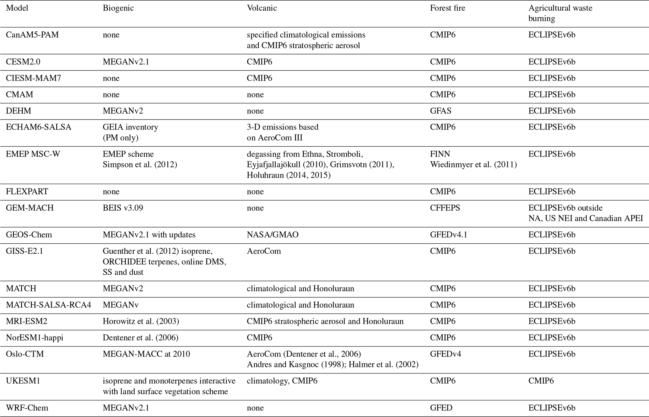
2.2 Chemistry
This section contains a summary of models' chemistry schemes, and we refer the reader to Appendix A and references therein for more details.
2.2.1 Methane
All participating models that provided CH4 output prescribed CH4 concentrations based on box model results from Olivié et al. (2021) for 2015 and from Meinshausen et al. (2017) for years prior to 2015. The former utilized the ECLIPSE v6B anthropogenic CH4 emissions (Sect. 2.1), along with assumptions for the natural emissions (Olivié et al., 2021; Prather et al., 2012), to provide as input to models' surface or boundary layer CH4 concentrations. Models then allow CH4 to take part in photochemical processes, such as the production of tropospheric O3.
2.2.2 Tropospheric chemistry
There is a wide range of tropospheric gas-phase chemistry implemented in the models. Air-quality-focused models, such as DEHM, EMEP MSC-W, GEM-MACH, GEOS-Chem, MATCH, and WRF-Chem, have detailed HOx–NOx–hydrocarbon O3 chemistry, with speciated volatile organic compounds (VOCs) and secondary aerosol formation. The GISS-E2.1, MRI-ESM2, and UKESM1 ESMs also use this level of tropospheric chemistry. In contrast, climate-focused models like CanAM5-PAM, CIESM-MAM7, ECHAM-SALSA, and NorESM1 contain bare minimum gas-phase chemistry and use prescribed O3 fields (e.g., CanAM5-PAM uses CMAM climatological O3 fields). The CCMs are somewhere in between, with simplified tropospheric and stratospheric chemistry so that they could be run for longer time periods. For example, CMAM's tropospheric chemistry consists only of CH4–NOx–O3 chemistry, with no VOCs.
2.2.3 Stratospheric chemistry
Only a subset of the participating models have a fully simulated stratosphere. CMAM, MRI-ESM2, GISS-E2.1, OsloCTM, and UKESM1 contain a relatively complete description of the HOx, NOx, Clx, and Brx chemistry that controls stratospheric ozone along with the longer-lived source gases such as CH4, N2O, and chlorofluorocarbons (CFCs). Other models have a simplified stratosphere, such as GEOS-Chem, which has a linearized stratospheric chemistry scheme (Linoz, McLinden et al., 2000), and WRF-Chem, which specifies stratospheric concentrations from climatologies – both of which do not simulate stratospheric chemistry. Finally, several models have no stratosphere or stratospheric chemistry at all (e.g., CIESM-MAM7, GEM-MACH, DEHM, and EMEP MSC-W).
2.2.4 Aerosols
Most models contain speciated aerosols: mineral dust (also known as crustal material), sea salt, BC, OA (sometimes separated into primary and secondary), SO, nitrate (NO), and ammonium (NH). However, some, like CanAM5-PAM and UKESM1, do not simulate NO and NH, but assume all is in the form (NH4)2SO. OA, SO, NO, and NH are involved in chemical reactions interacting with the gas-phase chemistry. Aerosol size distributions are either prescribed or discretized into lognormal modes or size sections. How the aerosol size distribution varies in space and time depends on many different processes, including emission, aerosol microphysics, aerosol–cloud interactions, and removal. How these processes are parameterized depends on the model, and we refer the reader to the Appendix and the references therein for more detail.
We have utilized many freely available observational datasets of SLCFs to evaluate the models. General descriptions are given below under the broad headings of surface monitoring, satellite, and campaign datasets, and there is some additional information in Appendix B.
3.1 Surface monitoring datasets
3.1.1 CH4 and O3
Global surface CH4 measurements were obtained from the World Data Centre for Greenhouse Gases (WDCGG). These measurements were made via gas chromatography, which has a < 1 % uncertainty range. Surface in situ O3 measurements are typically made via various types of UV absorption monitors, employing the Beer–Lambert law to relate UV absorption of O3 at 254 nm directly to the concentration of O3 in the sample air (e.g., Bauguitte, 2014), which have approximately a 3 % or 1–2 ppbv uncertainty range. We obtained surface O3 measurements from various networks: the National Air Pollutant Surveillance Program (NAPS) and the Canadian Pollutant Monitoring Network (CAPMON) for Canada, the Chemical Speciation Network (CSN) for the US, the Beijing Air Quality and Hong Kong Environmental Protection Agency for China, the Climate Monitoring and Diagnostics Laboratory (CMDL) for some global sites, the European Monitoring and Evaluation Programme (EMEP), and some individual Arctic monitoring stations like Villum Research Station and Zeppelin Mountain. Many of these measurements were downloaded from the EBAS database. The Arctic O3 measurement locations are shown in Fig. 1.
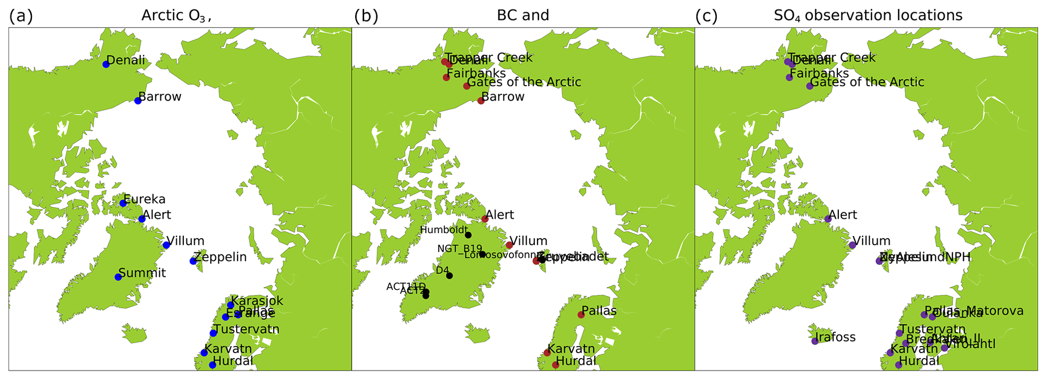
Figure 1Locations of Arctic surface in situ measurements, including (a) O3, (b) BC in brown, and ice cores in black, as well as (c) SO.
3.1.2 CO, NO, and NO2
CO and NOx measurements were obtained from the same monitoring networks as O3. CO instrumentation is similar to that for O3; however, it uses gas filter correlation to relate infrared absorption of CO at 4.6 µm to the concentration of CO in the sample air (Biraud, 2011). For NOx, the instrument deploys the characteristic chemiluminescence produced by the reaction between NO and O3, the intensity of which is proportional to the NO concentration. NO2 measurements are approximated using its thermal reduction to NO by a heated (350∘C) molybdenum converter (Bauguitte, 2014). Note that this method has an estimated bias of about 5 %–20 % because of sensitivity to other oxidized nitrogen species, and this has not been corrected for. The bias is on the lower end for high-NOx conditions and in the low-NOx Arctic can be up to 100 % uncertainty.
3.1.3 BC and OA
There are various BC measurement methods exploiting different properties of BC and thus measuring different quantities (Petzold et al., 2013): elemental carbon (EC) determined by thermal and/or thermal–optical methods, equivalent BC (eBC) by optical absorption methods, and refractory BC (rBC) by incandescence methods. Table B1 in Appendix B lists the different measurement techniques and instruments that the different monitoring networks and individual Arctic monitoring stations use. As BC emission inventories, including ECLIPSEv6b, are mainly based on emission factors derived from thermal and/or thermal–optical methods, modeled BC is consequently representative of EC.
The different types of BC measurements (EC, eBC, and rBC) usually agree with each other within a factor of 2 (AMAP, 2022; Pileci et al., 2021). However, it has been shown that, as the aerosol ages, the complex state of mixing of BC particles causes eBC to increase relative to EC (Zanatta et al., 2018). The absorption and scattering cross sections of coated BC particles vary by more than a factor of 2 due to different coating structures. He et al. (2015) found an increase of 20 %–250 % in absorption during aging, significantly depending on coating morphology and aging stages. Thus, this complexity impacts model–measurement comparisons at remote Arctic locations where one would expect eBC to have a high, positive uncertainty.
We obtained BC from the Canadian Aerosol Baseline Measurement (CABM) network for Canada, Interagency Monitoring of Protected Visual Environments (IMPROVE) network for the US, the EMEP network for Europe, and individual Arctic locations. To our knowledge, there were no other freely accessible BC measurements. The major observing networks EMEP, CABM, and IMPROVE measure EC with approximately 10 % uncertainty (Sharma et al., 2017). However, given the complexities in different BC measurement types, as mentioned above, the overall uncertainty is about 200 %.
Another complexity with model evaluation of BC is that some of the eBC measurements that models are compared to were made from collected particulate matter with different maximum diameters (e.g., PM1, PM2.5, and PM10). These are included in Table B1 for each of the measurement locations. From the models we use BC from PM2.5, as most of the BC is expected to be in the submicron mode.
Organic carbon (OC) is also measured via thermal and/or thermal–optical methods (Chow et al., 1993, 2001, 2004; Huang et al., 2006; Cavalli et al., 2010; Chan et al., 2019; Huang et al., 2021) using the same instrumentation as for EC detection in IMPROVE, CABM, NAPS, and EMEP measurement networks. These OC measurements have approximately 20 % or less uncertainty (Chan et al., 2019). Models output organic aerosol (OA), which includes OC and organic matter and is related to OC via a factor of 1.4 (Russell, 2003; Tsigaridis et al., 2014), though this factor has been reported as a range from 1.4 to 2.1 in the literature, depending on the source of OC and OA (Tsigaridis et al., 2014). Nevertheless, we applied a conversion factor of 1.4 to the OC measurements before comparing the modeled OA.
Arctic BC measurement locations are shown in Fig. 1, and many of these Arctic aerosol measurements were discussed in Schmale et al. (2022). We also evaluated modeled BC deposition by comparing it to BC deposition derived from ice core measurements (D4, ACT2: McConnell and Edwards, 2008; Humboldt: Bauer et al., 2013; Summit: Keegan et al., 2014; NGT_B19, ACT11D: McConnell et al., 2019). All of the ice core locations are also shown in Fig. 1. Deposition fluxes are not a measured value but are derived from the EC concentrations in ice and precipitation estimates.
3.1.4 SO
Surface in situ SO measurements in the major observing networks typically use ion chromatography methods, which have an approximately 3 % uncertainty range (Solomon et al., 2014). However, SO measurements have been shown to have up to 20 % analytical uncertainty (AMAP, 2022). SO datasets were obtained from IMPROVE, EMEP, and CABM networks, often via the EBAS database.
SO deposition was also derived from the same ice core measurements mentioned above for BC deposition (D4, ACT2: McConnell and Edwards, 2008; Humboldt: Bauer et al., 2013; Summit: Maselli et al., 2017; NGT_B19, ACT11D: McConnell et al., 2019). The Arctic SO measurement locations are shown in Fig. 1.
3.1.5 PM2.5
Surface in situ PM2.5 measurements are usually made via gravimetric analysis of particulate matter collected on a filter (e.g., Teflon substrate), which has around a 1 %–6 % uncertainty range (Malm et al., 2011). These data were obtained from Beijing Air Quality and US Embassy data for China, NAPS for Canada (Dabek-Zlotorzynska et al., 2011), IMRPROVE for the US, and EMEP and/or EBAS for Europe.
3.2 Satellite datasets
Satellite observations are useful for evaluating models on larger horizontal spatial scales and for evaluating the three-dimensional atmosphere – not the surface concentrations. Observations from three satellite instruments were used to evaluate model trace gas distributions in the free troposphere and, when appropriate, the lower stratosphere. These were the Tropospheric Emission Spectrometer version 7 (TES; NASA Atmospheric Science Data Centre, 2018; Gluck, 2004a, b), the Atmospheric Chemistry Experiment–Fourier Transform Spectrometer version 4.1 (ACE-FTS; Bernath et al., 2005; Sheese and Walker, 2020), and the Measurements of Pollution in the Troposphere version 8 (MOPITT; Ziskin, 2000; Deeter et al., 2019). The vertical profiles of trace gas volume mixing ratios are derived or retrieved from the satellite-measured emission or absorption spectra, with varying degrees of vertical sensitivity. These remote techniques typically have about a 15 % uncertainty in the measurements (e.g., Verstraeten et al., 2013), though this depends on the specific instrument and the species retrieved (e.g., Sheese et al., 2017).
Note that while TES and MOPITT have global spatial coverage, their coverage does not extend up into the high Arctic. The TES instrument on NASA's Aura satellite measures vertical profiles of trace gases such as O3, CH4, NO2, CO, and HNO from 2004–present. After interpolating all models and TES results to a 1∘ × 1∘ horizontal grid, the monthly mean CH4 and O3 from the TES lite products were matched in space and time with models. Models were smoothed with the TES monthly mean averaging kernels prior to comparisons with satellite data. TES measurements started in 2004, stopped in late 2015, and had poorer coverage in the last few years.
A similar comparison method was used for MOPITT data. The MOPITT instrument on NASA's Terra satellite measures CO from 2000 to the present.
The ACE-FTS instrument on CSA's SCISAT satellite has measured the trace gases O3, CO, NO, NO2, and CH4, among over 30 others from 2004–present. SCISAT has a high-inclination orbit, giving its instruments better coverage in the Arctic. ACE-FTS is a limb-sounding instrument measuring the solar absorption spectra of dozens of trace gas concentrations from the upper troposphere to the thermosphere. This gives us the opportunity to evaluate the 3-D model output in a region of the atmosphere where the radiative forcing of ozone is at its highest. Evaluating models with ACE-FTS measurements also provides insight into models' transport and upper-tropospheric chemistry. As was shown in Kolonjari et al. (2018), 3-hourly model output (rather than monthly mean output) is required for accurate comparisons to ACE-FTS data; thus, only models that provided output at this time frequency were compared to ACE-FTS measurements. The model output was sampled to match the times and locations of ACE-FTS measurements. We used an updated version of the advanced method in Kolonjari et al. (2018). Instead of taking the model output at the closest time to the ACE-FTS measurement time, the model output was linearly interpolated onto the ACE-FTS time. This reduces the bias introduced by diurnal cycles, which can cause certain volume mixing ratios (VMRs; e.g., that of NO and NO2) to vary significantly between model output times. As in Kolonjari et al. (2018), the model output is also interpolated vertically in log pressure space and bilinearly in latitude and longitude to account for spatial variation between model grid points.
3.3 Measurement campaigns
Finally, there were air- and ship-based measurement campaigns of black carbon that were used for model evaluation. Aircraft campaigns allow vertical profiles of chemical species to be evaluated, and ship campaigns allow for in situ measurements in the remote Arctic seas.
3.3.1 Aircraft campaigns
The flight paths of the aircraft used for model evaluation of BC are shown in Fig. 2. The aircraft campaigns include A-FORCE (Oshima et al., 2012), ARCPAC (Brock et al., 2011), ARCTAS (Jacob et al., 2010), EUCAARI (Hamburger et al., 2011), HIPPO (Schwarz et al., 2010), NETCARE (Schulz et al., 2019), and PAMARCMIP (Stone et al., 2010). Most of these aircraft campaigns occurred during boreal spring and summer months (April to July) except for one (HIPPO) occurring in January and November, and most occurred during the 2008–2009 time period, with only one (NETCARE) occurring during 2014–2015. All of these aircraft campaigns measured rBC from single-particle soot photometers (SP2) (Moteki and Kondo, 2010; Schwarz et al., 2006; Stephens et al., 2003).
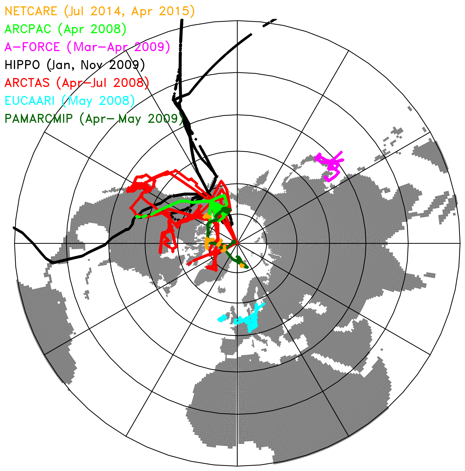
Figure 2Flight tracks of BC aircraft campaigns used in this study.
The AMAP models that submitted 3-hourly BC output were linearly interpolated onto the aircraft locations in space and time using the Community Intercomparison Suite (CIS; Watson-Parris et al., 2016) in order to provide representative comparisons and robust evaluation.
3.3.2 Ship campaigns
There were three ship-based measurement campaigns in 2014–2015. These were the two Japanese campaigns (MR14-05 and MR15-03 cruises of R/V Mirai) in September of 2014 and 2015 (track from Japan to north of Alaska; Taketani et al., 2016) and the Russian campaign in October 2015 (track north of Russia, from Arkhangelsk to Severnaya Zemlya and back; Popovicheva et al., 2017) – both are shown in Sect. 4.5 (Fig. 17). Models that provided 3-hourly BC output were compared to these observations. The Russian measurements of aerosol eBC concentrations were determined continuously using an Aethalometer purposely designed by MSU/CAO (Popovicheva et al., 2017). Light attenuation caused by the particles depositing on a quartz fiber filter was measured, and the light attenuation coefficient of the collected aerosol was calculated. eBC concentrations were determined continuously by converting the time-resolved light attenuation to the eBC mass corresponding to the same attenuation and characterized by a specific mean mass attenuation coefficient, in calibration with AE33 (Magee Scientific).
The Japanese measurements provide rBC (refractory BC). Pileci et al. (2021) showed that rBC and eBC are linearly related; thus, in order to compare the observations to models, we converted rBC to eBC via a factor of 1.8 (eBC = 1.8 × rBC; Zanatta et al., 2018; Pileci et al., 2021).
In this section, we evaluate modeled SLCFs from the 18 participating models with a focus on performance in the Northern Hemisphere midlatitudes (defined for our purposes as 30–60∘ N) and the Arctic (defined here as > 60∘ N for simplicity). Unless otherwise noted, the observations are compared to the model grid box that they are located in, and when more than one observation location occurs in the same model grid box, those observations are averaged first before the comparison. We look at spatial patterns in the model biases, as well as the vertical distribution and the seasonal cycles for each species, but first we start by providing a multi-species summary of the annual mean model biases in the surface air.
4.1 Multi-species summary
The 2014–2015 average modeled percent biases for surface concentrations of SLCFs are shown in Fig. 3 for each model and the multi-model mean (mmm). This figure is based on the model comparisons at the surface observation locations that will be shown in subsequent sections (Figs. 1, 5, 7, 10, 11, 13, 18, 21, and 23 and additional American observations from the IMPROVE network for BC, SO, and OA).
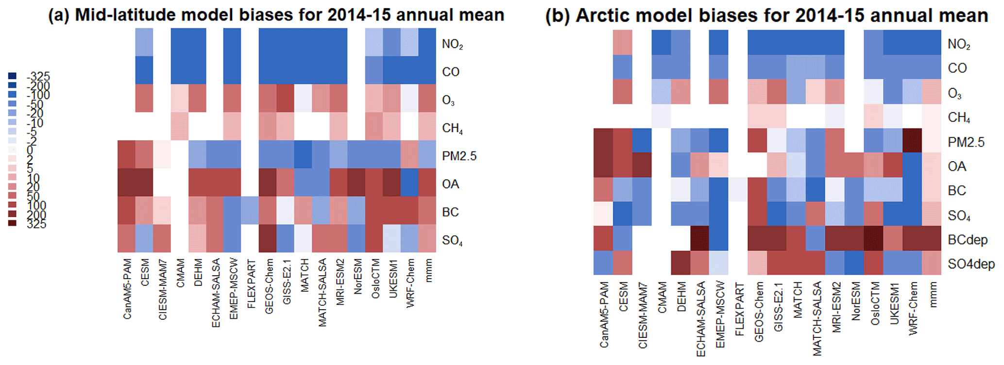
Figure 3Mean 2014–2015 model percent biases for each model and the mmm for surface SLCF concentrations as well as BC and SO deposition at (a) midlatitudes and (b) the Arctic. Note that the color scale is not linear.
Figure 3b shows that, for surface Arctic concentrations, no one model performs best for all species but that the mmm performs particularly well. It also shows that the model biases vary quite a bit among SLCF species for both the midlatitudes and the Arctic. It is important to note that there are many more measurement locations at midlatitudes compared to in the Arctic. BC, CH4, O3, and PM2.5 have the smallest model biases out of the SLCFs of this study, whereas OA, CO, and NO2 have larger model biases.
We find for half of the SLCF species that the mmm percent bias decreases with latitude (Fig. 4). O3, NO2, BC, and SO4 have a negative slope in the bias vs. latitude figure. So if the mmm bias was high at the midlatitudes, it is close to zero in the Arctic (O3), and if the mmm bias was near zero at midlatitudes, it is negative in the Arctic (NO2, BC, SO). This implies that there is not enough long-range transport from the midlatitude source regions to the Arctic. That said, the mmm CH4 bias stays relatively constant with latitude, and we will see in Sect. 4.2 that this result is model-dependent. The CO, PM2.5, and OA mmm biases have an increasing trend with latitude. However, both CO and PM2.5 have no observation locations in the high Arctic, so those results cannot represent long-range transport. OA only has one observation location in the high Arctic, and its bias is very large overall, so issues other than long-range transport are at play, as we will see in the following discussion (Sect. 4.7).
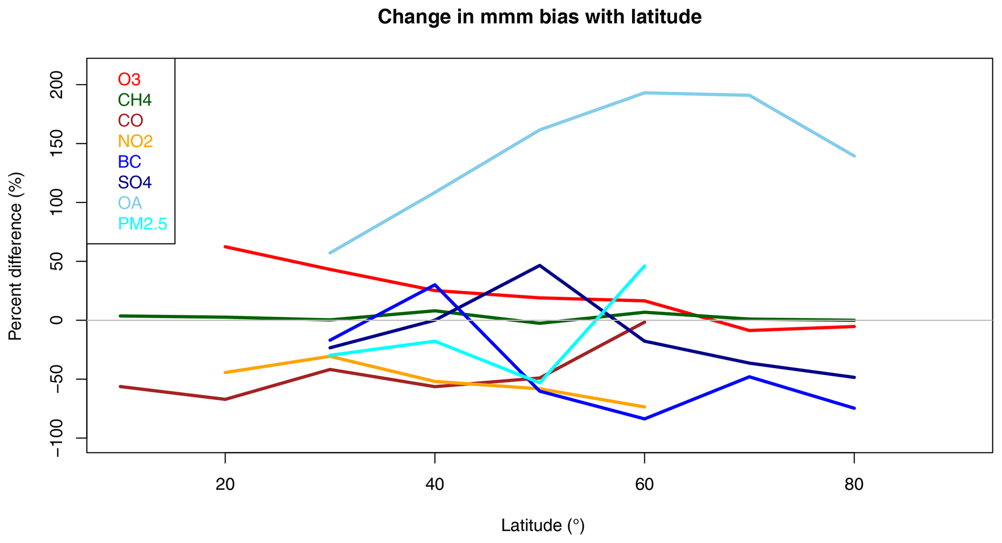
Figure 4Multi-model mean percent biases for surface SLCF concentrations versus latitude (in 10∘ latitude bins).
Of course, there are spatial, temporal, and model differences in the results, so we will now explore model performance for each SLCF in more detail in the next subsections.
4.2 Methane
Measured annual mean surface methane is shown in the top left panel of Fig. 5, along with model biases in the rest of the panels. Recall that unlike the rest of the SLCF species in this study, CH4 concentrations were prescribed in these models from the same CH4 dataset (Olivié et al., 2021). That said, the different decisions by modelers on how those CH4 global concentrations are distributed make differences in how these models compare to measurements. The mean model biases are small and mainly positive; in the midlatitudes, the multi-model mean bias is +145 ppbv (or +8.5 %), and in the Arctic, the mmm bias is 24 ppbv (or 1.3 %), which means that the models simulate the magnitude of surface CH4 well – though still outside the < 1 % measurement uncertainty range. There is a gradient in CH4 VMRs (higher in the Northern Hemisphere and lower in the Southern Hemisphere) that is seen in the measurements (Fig. 5, top left) and reported in the literature (e.g., Dlugokencky et al., 1994), though it is not well captured by CMAM, MRI-ESM2, and UKESM1 models, which are all biased low in the Northern Hemisphere and biased higher towards the south. That is because of the simplifications made in these models' distributions of CH4. For example, CMAM used a single global average CH4 concentration that is interpolated linearly in time from once-yearly values.
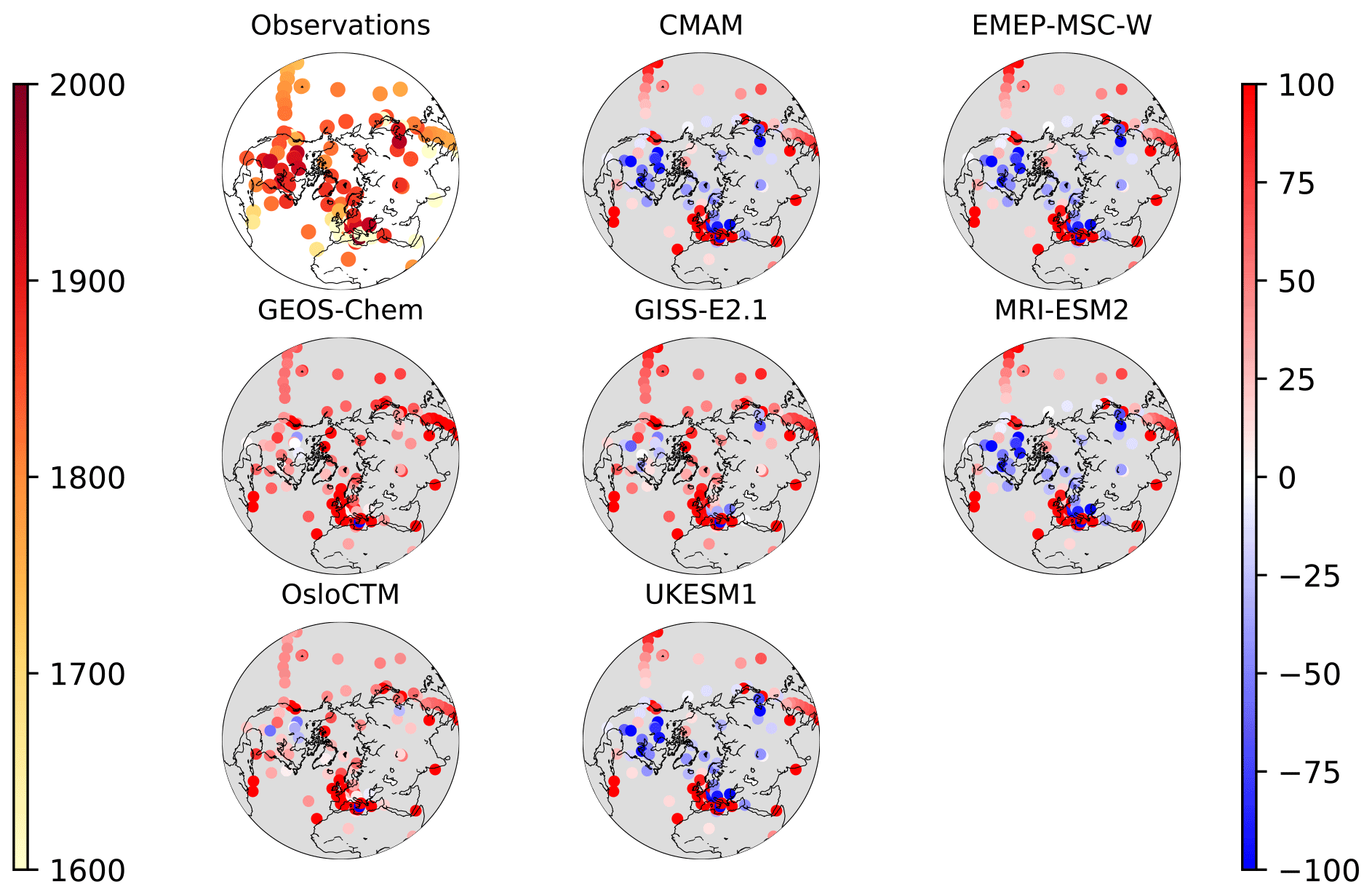
Figure 5Measured surface-level methane (top left) (ppbv, left color bar) and (remaining panels) model biases (model minus measurement, also ppbv, right color bar) for 2014–2015.
Figure 5 also shows that observed annual mean surface CH4 ranges geographically from about 1500 to 2100 ppbv depending on location; however, the models have a much smaller range due to their prescribing CH4 concentrations as a lower boundary input. For example CMAM CH4 volume mixing ratios only span about ±3 ppbv around 1836 ppbv. The span of MRI-ESM2 surface CH4 is even smaller. GEOS-Chem, GISS-E2.1, and OsloCTM have a more realistic range of 1700–2000 ppbv, though they still do not get the full variability that is seen in surface CH4 mixing ratios close to CH4 sources. However, in the free troposphere (above the boundary layer), we have TES satellite measurements of CH4 that show that CH4 is much more smoothly distributed aloft. Thus, the simplification of prescribing CH4 concentrations in the models is more realistic there (Fig. 6, showing the 600 hPa level in the mid-troposphere). Additionally, Fig. 6 better illustrates the latitudinal gradient in CH4 over the globe and its lack in some models, which have more negative biases in the Northern Hemisphere and more positive biases in the Southern Hemisphere. Other models, such as GISS-E2.1, do a good job of capturing the global distribution of CH4.
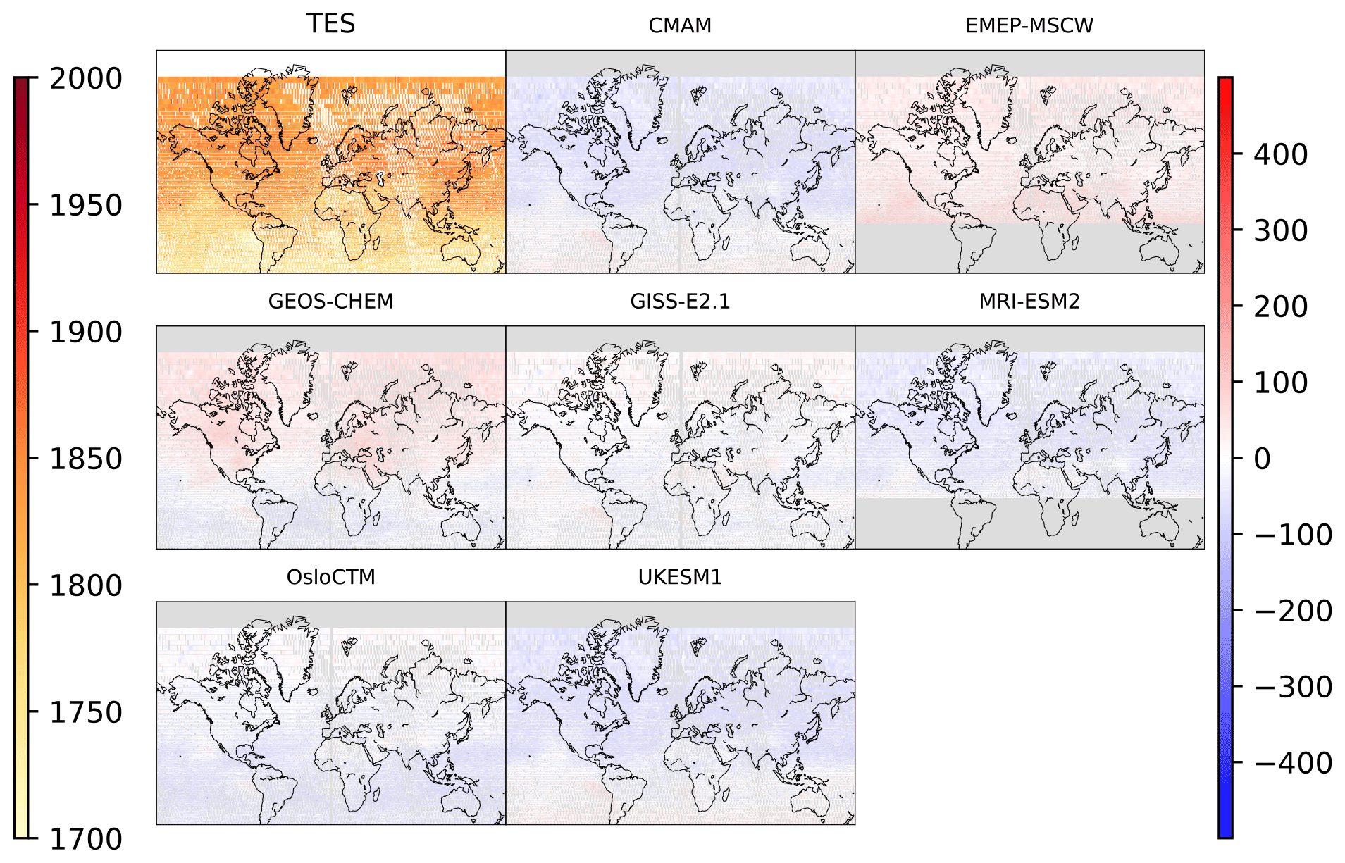
Figure 6TES measurements (top left) of CH4 in the mid-troposphere (at 600 hPa, ppbv, left color bar) and (remaining panels) model biases for 2008–2009 (model minus measurement, also ppbv, right color bar). Results for 2014–2015 are similar but had less spatial coverage by the satellite. Gray areas have no data (either from the model, TES, or both).
In the Arctic, the vertical cross section of CH4 VMRs over time as measured by the ACE-FTS in the middle to upper troposphere and in the stratosphere is shown in Fig. S1. There is a large decrease in CH4 above the tropopause at around 300–100 hPa. The models are all biased low around 300 hPa and high around 100 hPa. This pattern is true for midlatitudes as well as in the Arctic and may imply that the altitude of the modeled tropopause is too low. This same conclusion was also found in Whaley et al. (2022a) via comparisons of these models' simulations to ozonesonde measurements and in our satellite O3 comparison in the next section. The CH4 model–measurement correlation coefficients for ACE-FTS are relatively high (e.g., R=0.48 to 0.86 depending on the model).
Therefore, the general model evaluation for CH4 indicates that because models do not explicitly model CH4 emissions, they do not simulate the surface-level variability of CH4 VMRs. Models differ in their global distribution of CH4; thus, only some contain the north–south CH4 gradient. Those that do not have the largest underestimations of Arctic tropospheric CH4. The CH4 evaluation also implies that the modeled tropopause height may be too low.
4.3 Ozone
Tropospheric O3 is the third most important greenhouse gas (IPCC, 2021), and it is a regional pollutant that causes damage to human health and ecosystems. O3 is a secondary pollutant formed in the troposphere via photochemical oxidation of volatile organic compounds in the presence of nitrogen oxides (NOx= NO + NO2). As such, models must simultaneously simulate the meteorological conditions, precursor species distributions, and photochemistry correctly in order to accurately simulate O3. That said, since surface O3 is an important contributor to poor air quality, there is significant pressure for models to simulate it accurately, particularly in the heavily populated midlatitudes (e.g., for air quality forecasting). Only models with prognostic O3 are included in this section.
Figure 7 shows the in situ summertime mean O3 measurements (top left panel), and the model biases (remaining panels) and the same for the annual mean is shown in the Supplement (Fig. S2). These include averaging O3 from hourly observations (day and night) and 3-hourly or monthly modeled O3 depending on which were available for each model. Surface O3 is overpredicted by most models, which has been documented previously (Makar et al., 2017; Turnock et al., 2020). It has been shown that models can have problems producing low O3 overnight (Brown et al., 2006; Lin et al., 2008). In the Arctic, simulated surface O3 has more mixed results. Annual mean concentrations are of the order of 40 ppbv, and individual model biases range from −20 % to +52 % globally on average for 2014–2015. The multi-model mean has a bias of +11 % for the Arctic, but this is not uniformly spatially distributed. All models overestimated surface O3 in Alaska (mainly due to the overestimation of summertime concentrations, discussed below), and most models have too little O3 at the Greenland location and in northern Europe.

Figure 7Summertime (JJA) (top left) mean in situ surface O3 measurements (ppbv, left color bar) and (remaining panels) model biases for 2014–2015 (model minus measurement, also ppbv, right color bar). Results for 2008–2009 are similar but are not available for China.
The models were all able to represent the summertime peak in the midlatitude seasonal cycle (not shown). In contrast to the more polluted midlatitudes, where surface O3 peaks in the summertime due to photochemical production being at a maximum, Arctic O3 is more influenced by the Brewer–Dobson circulation, bringing a maximum of tropospheric O3 in the springtime due to photochemical production (Wespes et al., 2012), descent from the stratosphere, and more long-range transport of O3 to the Arctic. Figure 8, shows this springtime peak in both the western (a, longitude < 0∘) and eastern (b, longitude > 0∘) Arctic in the measurements. However, the models only capture that seasonal cycle in the eastern Arctic (Fig. 8b), implying that the models represent large-scale circulation and possibly stratosphere to troposphere exchange well. But it is interesting to note that the models that have sophisticated representation of stratosphere–troposphere exchange (such as CMAM, MRI-ESM2, UKESM1) do not particularly stand out as better performers in Fig. 8 compared to models that do not simulate the stratosphere (such as DEHM, MATCH, MATCH-SALSA). Thus, its impact on surface O3 may be very small.
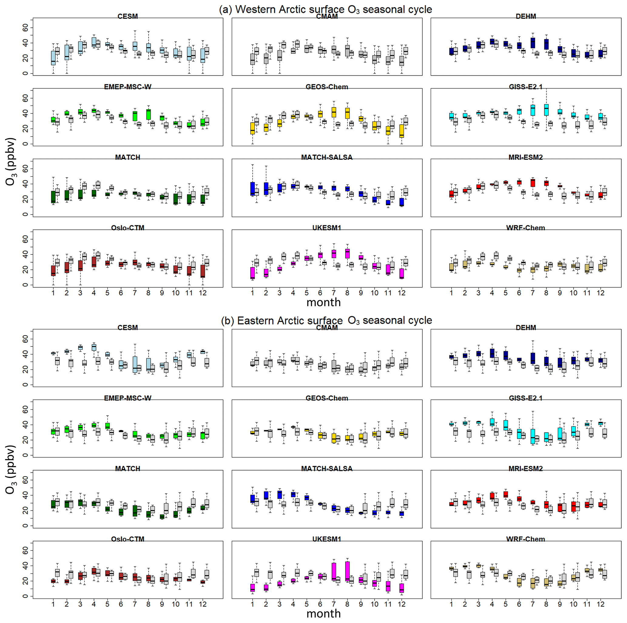
Figure 8Surface O3 monthly range that occurs at the locations in Fig. 7 above 60∘ N. The measurements are the black and white boxes and whiskers, and the models are the colored box and whiskers. (a) The western Arctic and (b) the eastern Arctic for 2014–2015. Thick horizontal lines indicate the median O3 VMR in each month, and the box extends to the interquartile range. The whiskers extend to the minimum and maximum monthly mean O3 VMR.
In the western Arctic (Alaska mainly, Fig. 8a), models overestimate summertime Arctic O3, likely due to overpredicting the impact of wildfire emissions on tropospheric O3 concentrations, which is a research topic with high uncertainty (van der Werf et al., 2010; Monks et al., 2015; Arnold et al., 2015). Another possibility is that modeled O3 dry deposition over boreal vegetation is underestimated (Stjernberg et al., 2012; Thorp et al., 2021).
Some Arctic locations are more inclined to get springtime surface O3 depletion due to bromine explosions and halogen chemistry (Bottenheim et al., 1986; Barrie et al., 1988; Simpson et al., 2007). None of the model simulations in this study contain the necessary tropospheric halogen chemistry to simulate those events, which partly explains why some models in Fig. 8 (bottom) overestimate springtime O3 concentrations. That particular feature is explored further on a site-to-site basis in Whaley et al. (2022a).
The next subsection shows that both the O3 precursors CO and NO2 are underestimated compared to measurements at all global locations. This has implications for simulated tropospheric O3 chemistry.
Free-tropospheric O3 – satellite comparisons. Aircraft-based measurements and ozonesondes can provide insight into the vertical distribution of O3, and these have been well documented (e.g., Tarasick et al., 2019; Whaley et al., 2022a). However, model grid boxes may not be representative of those fine-spatial-scale measurements. In this study, we examine how the model biases change in the vertical when compared to satellite measurements, which have a larger, “smoothed out” spatial sensitivity due to their viewing geometry and retrieval methods. Specifically, we compare modeled O3 to TES and ACE-FTS satellite-based retrievals. These satellite instruments also have better global coverage than aircraft and sonde-based measurements.
The model fractional biases compared to TES measurements from near the surface up to 100 hPa are shown in Fig. 9 for the Arctic (left) and midlatitudes (right). All models' simulated fractional biases have similar vertical profiles for both the Arctic and midlatitudes, with greater negative values at lower levels and a more positive “bulge” of about 10 % around 300 hPa in the Arctic and about 5 % around 200 hPa at midlatitudes. That bulge in model biases at 300 hPa was also seen to a greater degree (50 %–70 %) when comparing these model simulations to Arctic ozonesonde measurements in Whaley et al. (2022a). Compared to TES, which has much lower vertical resolution, the results are not as striking but are consistent with ACE-FTS measurements. On average, the models have a negative bias at all vertical levels in the Arctic region and in lower troposphere in the midlatitude region, whereas a positive bias is seen in the upper troposphere below 60∘ N. This is consistent for the two time periods (2008–2009 and 2014–2015).
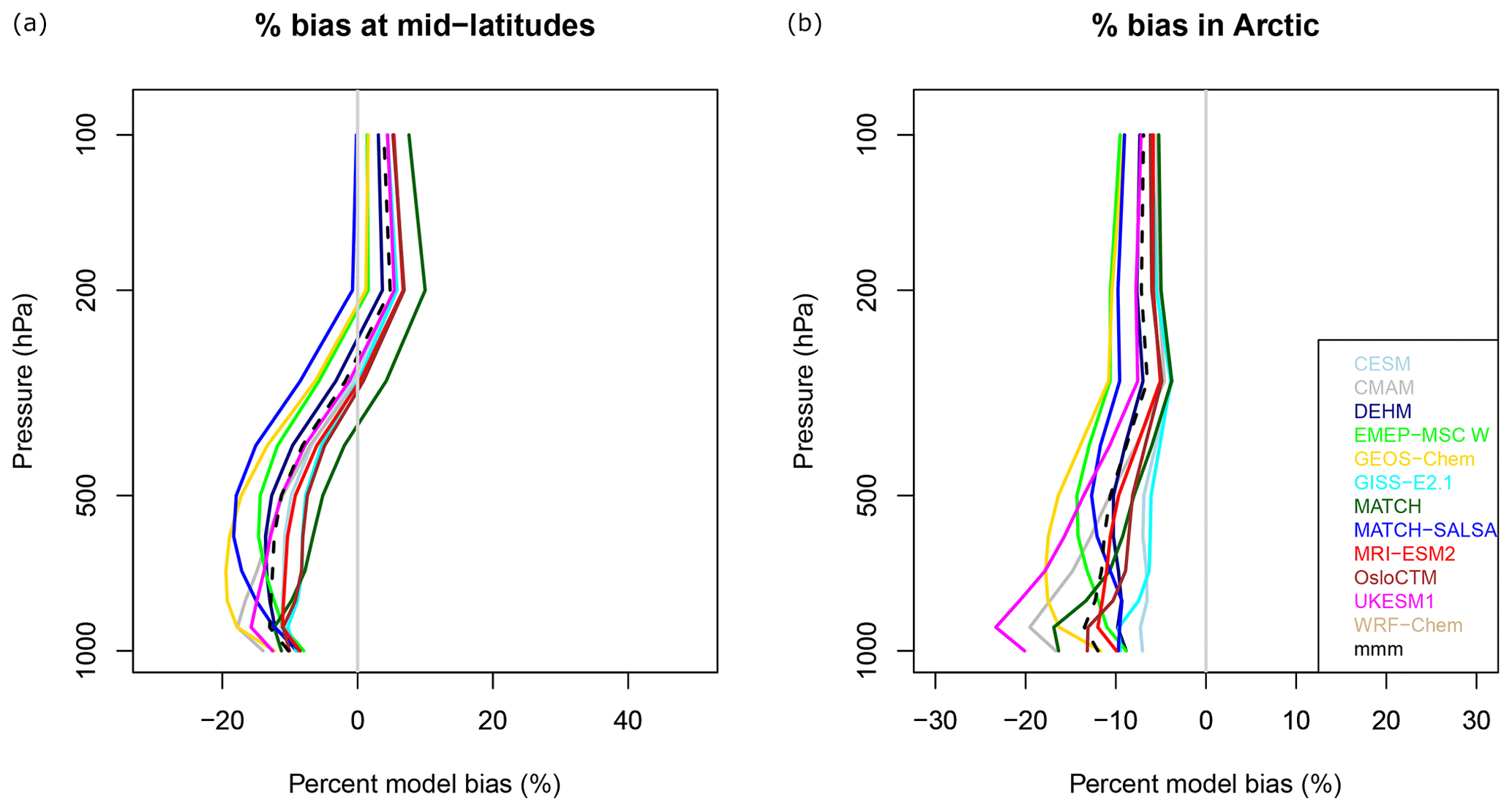
Figure 9Vertical distribution of models' O3 percent biases (model minus measurement over measurement) for 2008–2009 compared to the TES measurements; (a) average for midlatitudes (30–60∘ N) and (b) average for Arctic latitudes (> 60∘ N).
Given that Fig. 7 shows positive biases near the midlatitudes, while Fig. 9 shows lower O3 in the free troposphere, these results imply that there is not enough vertical lifting and/or mixing of tropospheric O3 in most of the models. However, the TES measurements have been shown to be biased high by approximately 13 % throughout the troposphere (Verstraeten et al., 2013), which is the same amount that the mmm is low. Similarly, ACE-FTS O3 has an uncertainty range of +5 %–10 % when compared to O3 from other satellite limb-view observations (Sheese et al., 2017). The ACE-FTS comparison for O3 can be found in the Supplement (Fig. S3), showing higher model biases around 300–100 hPa (except for GEOS-Chem) and good agreement below that. Therefore, overall, participating models simulate the free-tropospheric O3 reasonably well and within the uncertainly limits of the observations.
Therefore, the general model evaluation for O3 indicates that all models overestimate surface O3 at midlatitudes, and that, combined with a lack of O3 transport to the Arctic, results in modeled Arctic O3 VMRs having relatively little bias (the right answer for the wrong reason). The summertime evaluation implies that models overestimate the O3 produced and transported by wildfires in the western Arctic. The O3 evaluation also implies that the modeled tropopause height may be too low.
4.4 O3 precursors: carbon monoxide and nitrogen oxides
Figures 10 and 11 show the comparisons of the multi-model medians (MMMs) to the surface in situ measurements. The figures for each model appear in the Supplement (Figs. S4 and S5), but only the MMMs are shown here since the spatial patterns were very similar for all models. The multi-model annual mean underpredicts both CO and NO2 by approximately −55 % in the Northern Hemisphere for 2014–2015. The 2015 AMAP report showed similar findings for simulated surface CO, as have other studies (AMAP, 2015a; Emmons et al., 2015; Monks et al., 2015; Jiang et al., 2015; Quennehen et al., 2016), pointing to a likely underestimation of CO emissions and possibly shorter modeled lifetimes of CO due to an overestimation in OH (Miyazaki et al., 2012). The annual mean surface CO underestimation is mainly dominated by the wintertime (e.g., the mmm bias in DJF is −92 %), when it has been reported that CO emissions from combustion are too low (e.g., Kasibhatla et al., 2002; Pétron et al., 2002). All the models exhibit a large negative bias over China, which is consistent with the study by Quennehen et al. (2016) and is attributed to the enhanced destruction of CO by OH radicals, but it was also found in Kasibhatla et al. (2002) and Pétron et al. (2002) that bottom-up CO emission inventories in Asia are greatly underestimated.
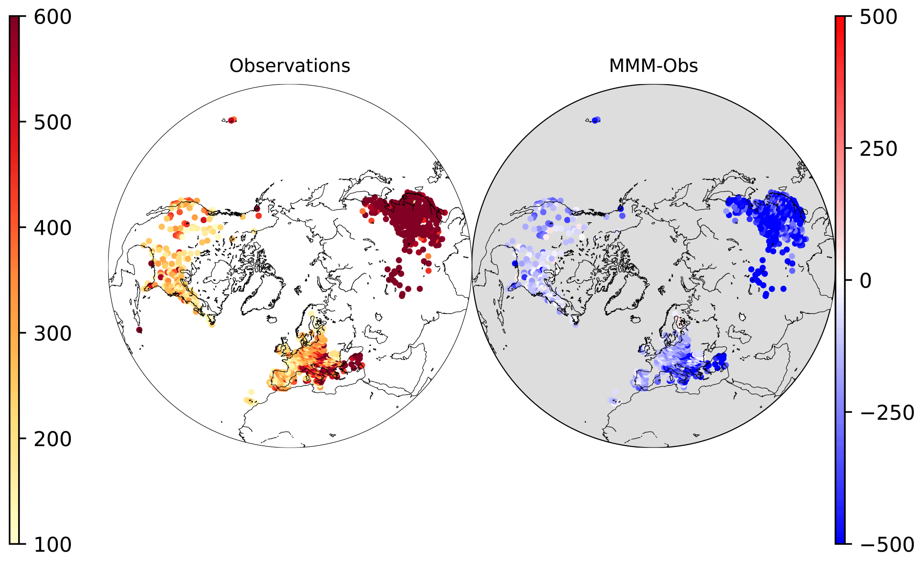
Figure 10Mean CO volume mixing ratios (ppbv, left color bar) at surface measurement sites and MMM bias (MMM minus measurement ppbv, right color bar) for 2014–2015. Results from 2008–2009 are similar and not shown.
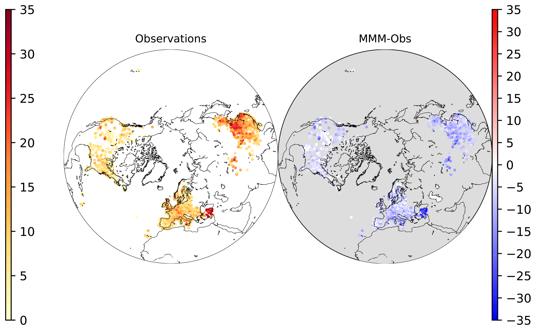
Figure 11Mean NO2 volume mixing ratios (ppbv, left color bar) at surface measurement sites and MMM bias (MMM minus measurement in ppbv, right color bar) for 2014–2015. Results from 2008–2009 are similar and not shown.
In the free troposphere, we compare modeled CO to that measured by MOPITT. Figure 12 shows these comparisons for the summertime (JJA) mean at the 600 hPa level, and Fig. S6 in the Supplement shows the same for the springtime (MAM) mean. Unlike in the winter and spring when all models are biased low at midlatitudes, there is more variability in the summertime biases, with about half the models overestimating free-tropospheric CO and the other half underestimating it. In the Arctic region, all models are biased high in the summer but low in the springtime. In the winter, MOPITT does not have coverage in the Arctic. Monks et al. (2015) discussed the fact that models had high biases in the tropospheric column of CO compared to MOPITT measurements in the outflow from Asia and low biases north of there due to lack of transport. The Quennehen et al. (2016) study also suggested that summertime CO transport out of Asia is too zonal when comparing models to IASI CO columns. At 600 hPa, where CO concentrations are lower and the atmosphere is more mixed, these features do not appear.
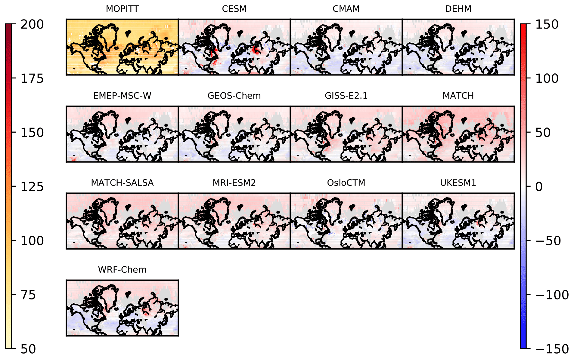
Figure 12Summertime (JJA) (top left) mean MOPITT CO at 600 hPa (ppbv, left color bar) and (remaining panels) model biases (model minus measurement ppbv, right color bar) for 2014–2015.
In the upper troposphere and stratosphere, modeled CO and NOx monthly time series are compared to measurements from the ACE-FTS satellite instrument (where NOx= NO + NO2, which are measured separately), and those results are shown as Taylor diagrams in Fig. S7, along with O3 and CH4 at 150 hPa, which is in the upper troposphere–lower stratosphere (UTLS) region. The contours show the model's overall skill as defined in Hegglin et al. (2010). Only the models that simulate the stratosphere were included, and the results show that there is a range in model performance by SLCF species, with no one model performing best for all. Comparison statistics for CO were poorer than those for O3, CH4, and NOx.
4.5 Black carbon
In this section, we examine the spatial and seasonal distributions of BC using ground-based measurements, which are primarily available in North America, Europe, and several locations in the Arctic, but are also available from two ship-based campaigns and several aircraft campaigns. Given the limited global data available for both BC and SO (e.g., we could find none freely available for Asia), we focus the plots on the Arctic region here, and given that the magnitude of BC and SO does not span a wide range throughout the Arctic, we show model biases as percent rather than absolute differences as was done in previous sections for trace gas species shown globally. We also analyze the BC model–measurement comparisons, keeping in mind that because there are various definitions and measurement types for BC, we consider agreement within a factor of 2 to be within the uncertainty range (Sect. 3.1.3).
Figure 13 (top left panel) shows annual mean surface-level concentrations of black carbon (BC) at nine Arctic observation stations and (remaining panels) the model percent biases there. The annual mean BC concentrations are of the order of less than 1 µg m−3, and most models tend to underestimate BC in the high Arctic while overestimating in Alaska and Scandinavia. This result could be partially explained by the discrepancy caused by the use of EC and eBC data, which are not the same (Sect. 3.1.3). As aerosols age during transport to high-Arctic locations, their eBC (based on absorption converted to mass) gets more and more of a positive bias compared to EC. As models are more representative of EC, they will not be able to agree with eBC measurements in aged air at high-Arctic remote stations, such as Gruvebadet, Zeppelin, Alert, and Utqiaġvik. This is in contrast to the Alaskan and European stations, which are closer to sources where BC is more fresh; thus, the eBC measurements have lower uncertainty.
That said, a few models (CanAM5-PAM, DEHM, and FLEXPART) overestimate BC concentrations in the high Arctic. Overall individual model biases range ±100 % at individual sites.

Figure 13Mean BC concentrations (µg m−3, top color bar) at surface Arctic measurement sites and model bias (as (model–measurement) measurement in percent, bottom color bar) for 2014–2015. Results from 2008–2009 are similar and not shown.
The underestimation of high-Arctic atmospheric BC concentrations may be related to excessive BC deposition further south; however, there are very few BC deposition measurements. In the Arctic, we can evaluate total (wet + dry) modeled deposition via derived ice core measurements. There were six ice cores on Greenland and one in the European Arctic in Spitsbergen (Lomosovfonna). Figure 14 shows that all models overestimate BC deposition fluxes at the ice core locations. While the ice cores contain BC data starting in the year 1750, only data after 1990 have been used to match the modeled time period (1990–2015, 1995–2015, 2008–2009, and 2014–2015, depending on the model).
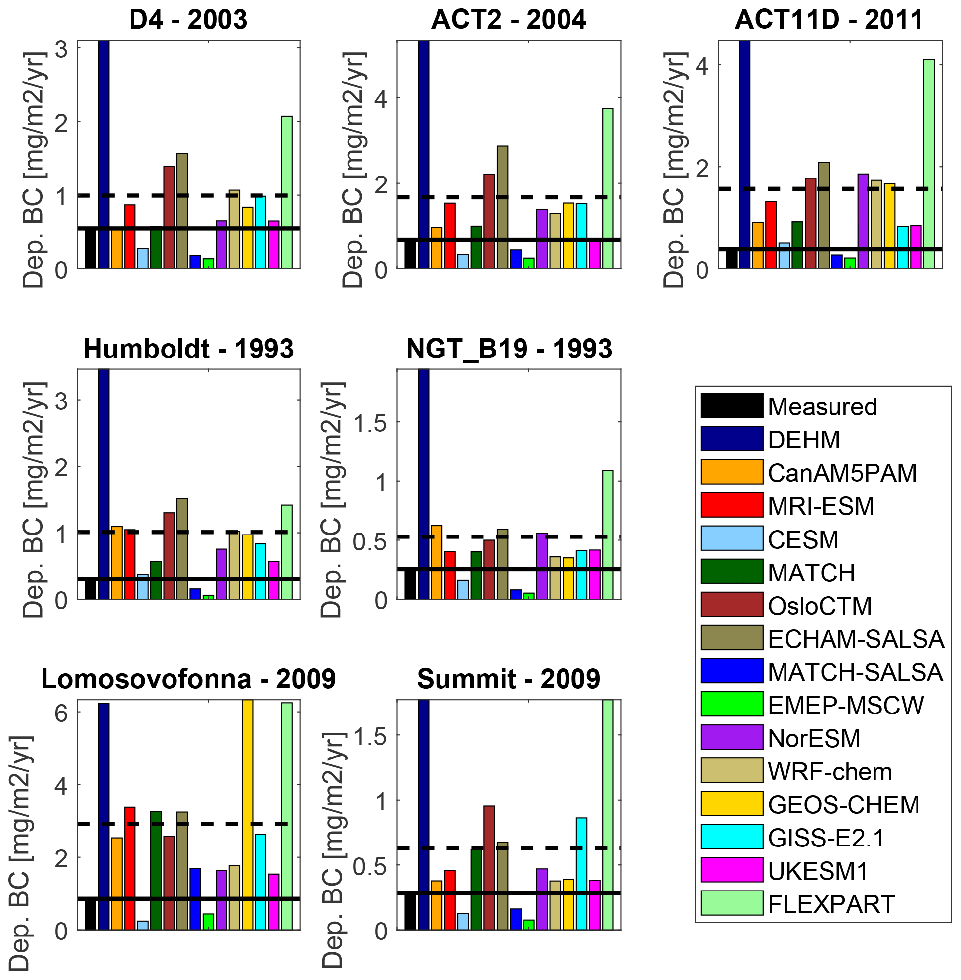
Figure 14Annual average BC deposition flux values for the seven ice core locations (Fig. 1b) for each model based on values from 2008–2009 and 2014–2015. The observed fluxes are plotted in black, and a black line indicates the level of the average observed flux; the black dashed line is the model mean for each location. The period used for plotting is based on all available years after 1990; the title indicates the last available year form the ice core record.
The measured BC deposition flux values on Greenland vary with elevation (lower fluxes at higher elevation). Summit (3177 m a.s.l.) has an average of 285 µg m−2 yr−1 in contrast to ACT2 (2461 m a.s.l.) with 676 µg m−2 yr−1. BC deposition is highest in the European Arctic at Spitsbergen with 856 µg m−2 yr−1. For all seven ice cores used in this comparison the averaged model mean is 3 times as high as the observations. At D4 (2728 m a.s.l.) the modeled mean corresponds best to the observation, with a mean bias of +83 %. At ACT11 (2296 m a.s.l.) the models have 4 times the deposition flux compared to the measurements. Generally though, the model mean is skewed higher by FLEXPART and DEHM (Fig. 14), which also had higher atmospheric BC concentrations. A few models simulated less BC deposition than observed at these sites, and these models also underestimated BC atmospheric concentrations. Thus, it is difficult to conclude that deposition biases are a cause for atmospheric biases when the two are inter-related parameters.
The seasonal cycles of surface-level atmospheric BC concentrations at several Arctic locations are shown in Fig. 15. As seen in Eckhardt et al. (2015), some models still underestimate wintertime BC, but many models now show similar seasonality as the observations. The multi-model mean also captures the monthly variations well including the summertime peak at some Alaskan sites caused by fire emissions. The multi-model mean Arctic BC is underestimated in winter (−24 %) and overestimated in the summer (+32 %), though overall, this is an improvement in model performance in simulating Arctic BC since the 2015 AMAP assessment of black carbon and ozone as climate forcers – the latter of which had −59 % winter bias and +88 % summertime bias (AMAP, 2015a; Eckhardt et al., 2015). However, it is difficult to make direct comparisons to that report as those values were for a smaller set of Arctic locations, different observation periods, and with a different set of models (though many overlapping). The model improvement may be due to the improved anthropogenic emissions of BC, particularly from northern Russia, where flaring emission factors were increased in ECLIPSEv6B compared to those used for the 2015 AMAP report.
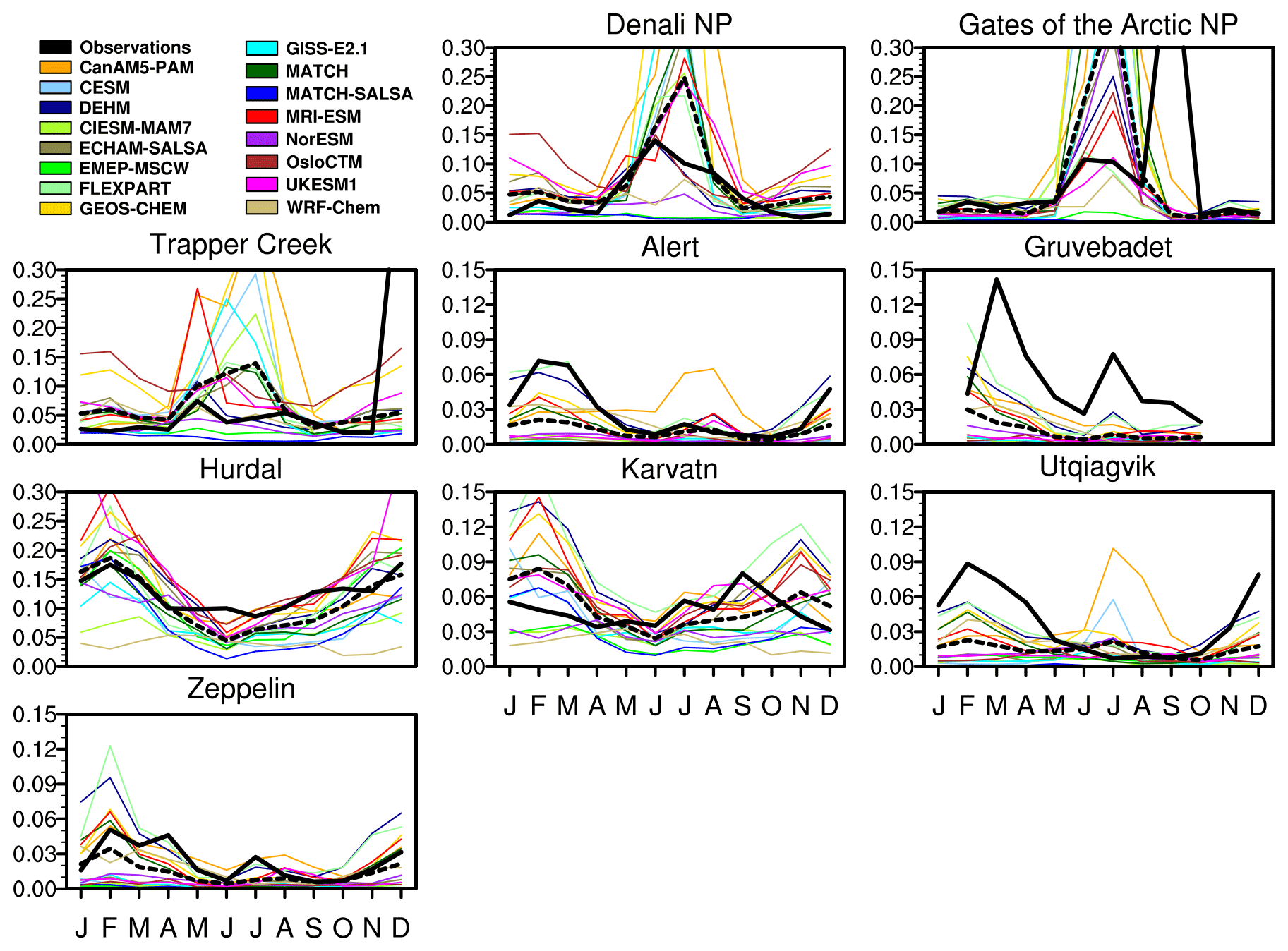
Figure 15Modeled (thin colored lines) and measured (thick black line) monthly mean BC concentrations (in µg m−3) at surface Arctic measurement sites in 2014–2015. The multi-model mean is shown by the black dashed line.
Most models have reasonable spatial correlation with the measurements across the Arctic in that they correctly simulate the range of BC concentrations that appear across the Arctic (e.g., higher concentrations at Hurdal, lower concentrations at Zeppelin), as shown in Fig. S8. However, there are still large differences and low R values in the statistics shown in Fig. S8.
There are positive model biases at midlatitudes (in North America and Europe; not shown) for surface-level BC. The vertical analysis of BC from the aircraft campaigns (below) provides further insight and support for the suggestion that models do not have adequate long-range transport of the pollutants from their sources in the midlatitude; thus, they do not simulate enough pollution in the Arctic.
Vertical profiles of BC – aircraft campaigns. Gridded BC output at 3-hourly intervals was provided by 11 of the participating models and was compared to aircraft campaign measurements of BC. The interpolation of model output to flight track coordinates was carried out by tools from the Community Intercomparison Suite (CIS; Watson-Parris et al., 2016), which co-located the extracted model tracks with their corresponding observational values.
Figure 16 shows the median vertical profiles of BC concentrations from the aircraft measurements and from the models. At midlatitudes, from 0–2 km, all of the models agree well with the measurements. However, BC concentrations decline steeply in a few models (e.g., MATCH-SALSA, EMEP-MSC-W, and GEOS-Chem) above 2 km. It would appear that they do not have enough vertical lifting of BC and/or perhaps too short of a BC lifetime. Indeed, one of these is EMEP MSC-W, in which the short BC lifetime was previously reported in Gliß et al. (2021). That said, in Lund et al. (2018b), the Oslo-CTM and ECHAM models were shown to overestimate the BC lifetime. In our case, OsloCTM is not shown in Fig. 16 because it did no provide BC at 3-hourly timescales. But ECHAM-SALSA results are consistent with the Lund et al. (2018b) study in that they particularly overestimate BC in the upper altitudes in both the midlatitudes and the Arctic, implying too long a lifetime and too much long-range transport into the upper Arctic atmosphere. The measured BC profile at midlatitudes drops off more quickly around the tropopause at 11–12 km, and, except for CanAM5-PAM, the models do not reproduce this drop.
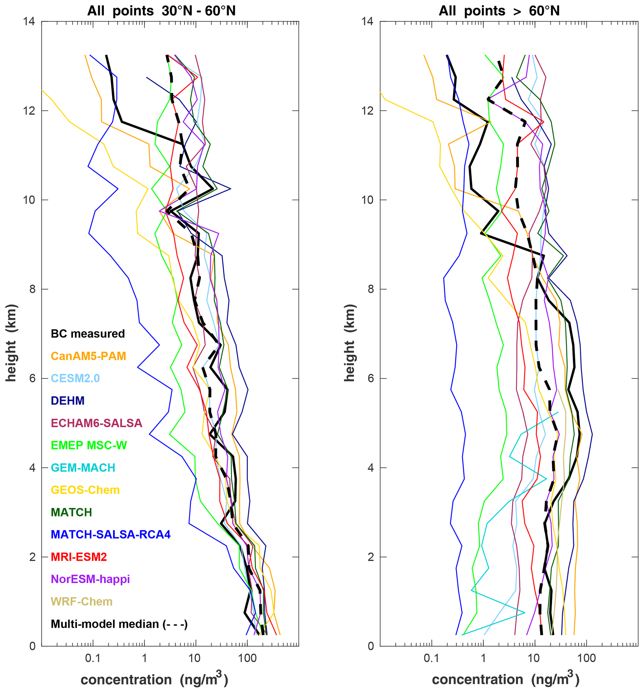
Figure 16Median vertical profiles of observed (heavy black line) and modeled (colored lines) BC concentrations for all aircraft campaigns combined, separated into (left) midlatitudes and (right) the Arctic. The multi-model median is shown by the dashed black line.
In the Arctic profiles (Fig. 16), the modeled and observed profiles do not decline with altitude throughout the troposphere, but the observed median BC concentration does drop sharply around 9 km – again near the Arctic tropopause, and again, the only model to capture that change is CanAM5-PAM. In the Arctic comparisons, the models that did not simulate enough BC aloft at the midlatitudes stand out as having larger underestimates of BC in the Arctic. For example, MATCH-SALSA and EMEP MSC-W have very low BC throughout the Arctic vertical profile. These results are consistent with the surface BC underestimation in Fig. 15. Therefore, the underestimation seen in the Arctic for those two models is likely due to a lack of long-range transport from the midlatitudes, as well as errors in BC deposition mentioned above. In addition, the Zhao et al. (2021) study showed that different parts of the Arctic BC vertical profile are sensitive to BC transported from different areas of the world. For example, the lower-tropospheric BC is influenced by emissions transported from North America, Russia–Belarus–Ukraine, Europe, and East Asia, whereas upper-tropospheric Arctic BC is mainly influenced by transport from South Asia. Thus, the differences in the model results could be related to differences in how they simulate these transport pathways.
Mahmood et al. (2016) found that, overall, considerable differences in wet deposition efficiencies in the models exist and are a leading cause of differences in simulated BC burdens. Results from their model sensitivity experiments indicated that convective scavenging outside the Arctic reduces the mean altitude of BC residing in the Arctic, making it more susceptible to scavenging by stratiform (layer) clouds in the Arctic. Consequently, scavenging of BC in convective clouds outside the Arctic acts to substantially increase the overall efficiency of BC wet deposition in the Arctic, which leads to low BC burdens compared to simulations without convective BC scavenging. Oshima et al. (2013) also found that convective scavenging at middle and subtropical latitudes removes a significant fraction of BC. In contrast, BC concentrations in the upper troposphere are only weakly influenced by wet deposition in stratiform clouds, whereas lower-tropospheric concentrations are highly sensitive (Mahmood et al., 2016) – these are consistent with the results we find in this study, wherein the multi-model median is too high above about 9 km and too low from 0–9 km. Indeed, the MATCH and MATCH-SALSA models, for example, assume reduced scavenging of aerosol in mixed-phase clouds following Liu et al. (2011), which increases long-range transport to the Arctic. It is odd then that MATCH is one of the better=performing models in Fig. 16 and MATCH-SALSA is not. Despite the large range in modeled vertical BC concentrations, the multi-model median is close to the observed throughout the troposphere at both midlatitudes and in the Arctic.
Arctic seas analysis – ship campaigns. From the ship-based measurements, we see that there is a consistent model overestimate of BC in the Pacific region (Japan cruise) where measured concentrations are very low (Fig. 17). Indeed, Taketani et al. (2016) report that BC concentrations were in the range 0–66 ng m−3, with an overall mean value of just 1.0 ± 1.2 ng m−3. The models, possibly due to their coarse resolutions, were not able to simulate such low background BC concentrations. However, even the model with the highest resolution (GEM-MACH at 15 km resolution) overestimated BC in the Pacific – though that limited-area model in that region near the boundary would have been heavily influenced by the upwind, coarser-resolution boundary conditions that were assumed (1∘ × 1∘ MOZART4 chemical boundary conditions). The high bias in the Pacific may be due to all models overestimating the amount of BC that gets transported off the Asian continent. That model bias is consistent with our low-altitude comparisons of the models to the HIPPO aircraft campaign measurements, which were taken over the northwestern Pacific (Fig. 2). The BC overestimate over the Pacific was also found in the Schwarz et al. (2013) study looking at simulated BC from the AeroCom global model intercomparison initiative compared to HIPPO measurements.
Conversely, the modeled BC concentrations generally agree with measurements in the Russian Arctic Ocean, though they are biased slightly low for the most part. Popovicheva et al. (2017) attribute the higher BC concentrations measured near the Kara Straight (north of 70∘ N) to gas-flaring emissions, and near Arkhangelsk (White Sea), important sources were midlatitude biomass burning, transportation, and combustion (residential and commercial). Since models were able to simulate this well, their improvement is likely due to improved Russian anthropogenic emissions in ECLIPSE v6B (Sect. 2.1, AMAP, 2022) compared to previous emissions datasets, which did not include enough Russian flaring emissions. The best model results were from ECHAM-SALSA and MATCH when compared to all of the ship campaign data.
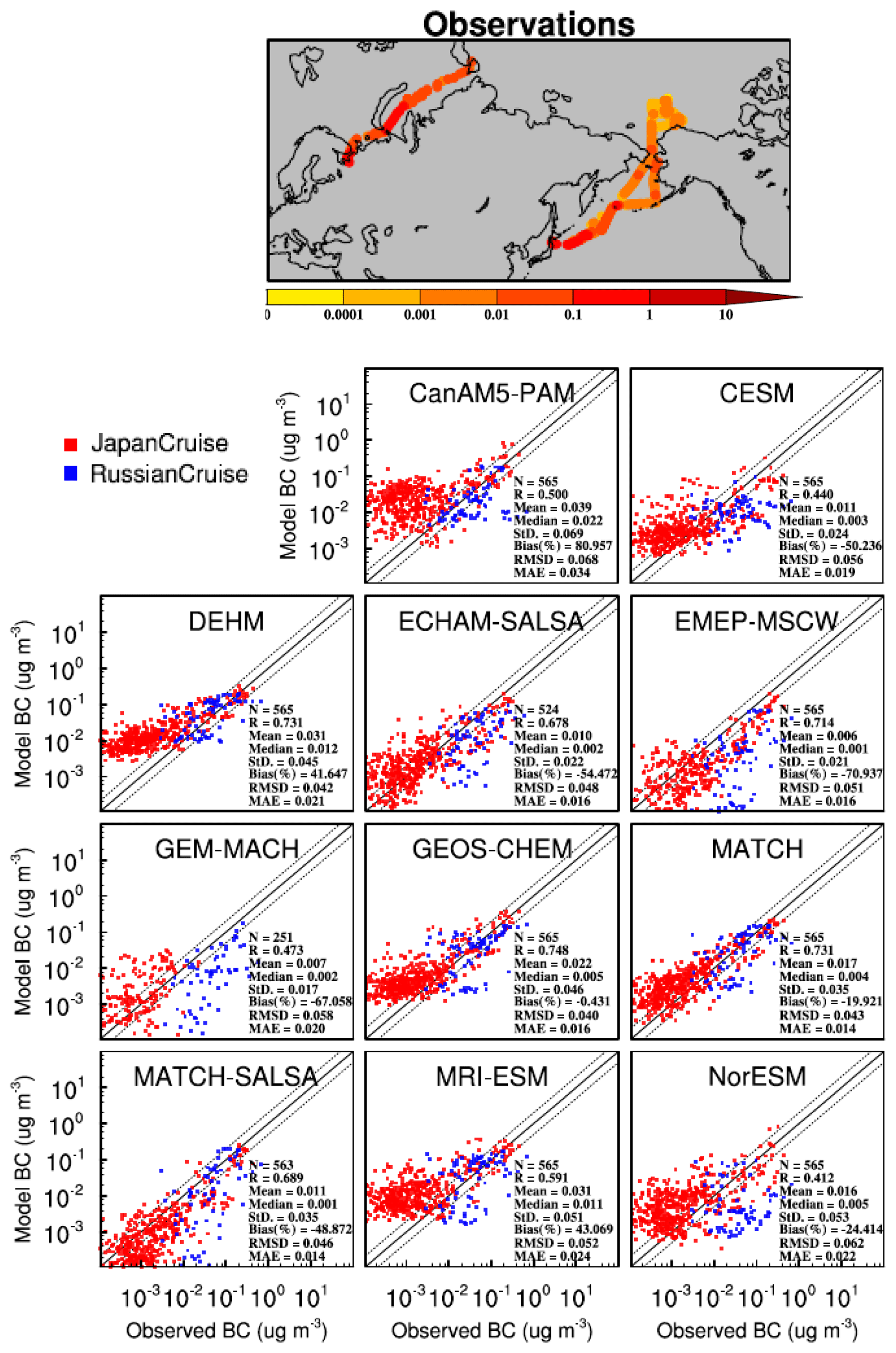
Figure 17Observed BC concentrations (top) (µg m−3, top color bar) along the ship paths and (remaining panels) the modeled vs. measured 3 h average BC concentrations along the ship paths. Note the logarithmic scale.
Therefore, the general model evaluation for BC indicates that while there is a large variability in models results, they tend to overestimate surface BC at midlatitudes (including over the Pacific Ocean) and underestimate surface BC in the Arctic. Again, these results point to a lack of transport to the Arctic and, in this case, too much BC deposition along the way. While we were only able to evaluate BC deposition in the Arctic in this study, those results support the hypothesis of some models having too much BC deposition. The BC vertical profile evaluation also implies that the modeled tropopause height may be too low.
4.6 Sulfate
We used monthly mean surface level observations of SO from 18 Arctic sites to evaluate the models. Figure 18 shows that, similar to BC, the SO concentrations in the high Arctic are underestimated by most of the models. A few models overestimate SO in Scandinavia and Alaska.
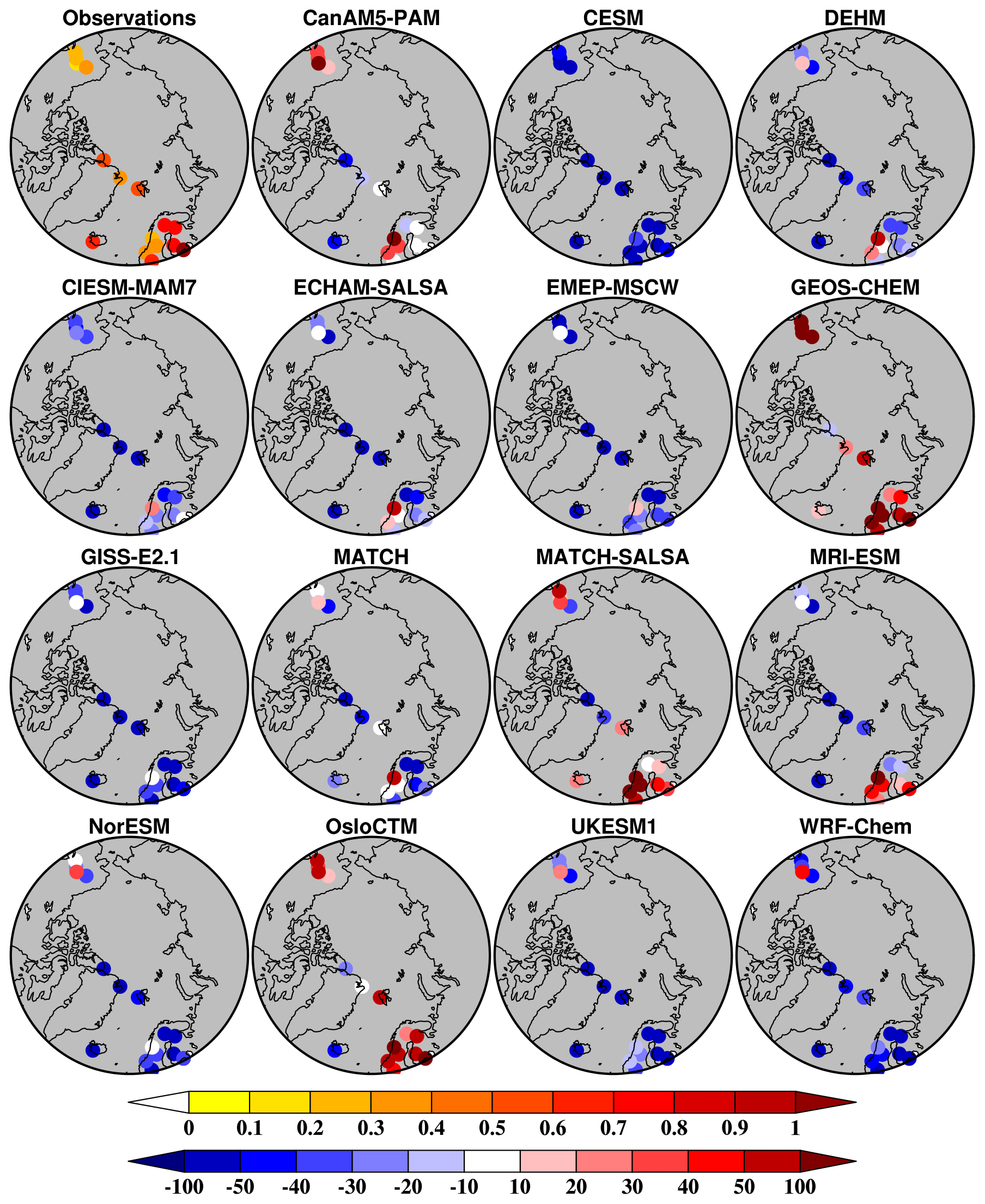
Figure 18Mean measured SO concentrations (µg m−3, top color bar) at surface Arctic measurement sites and model bias (as model–measurement measurement in percent, bottom color bar) for 2014–2015. Results from 2008–2009 are similar and not shown.
The model underestimations of SO could be mainly due to higher efficiencies of models in removing aerosol during the long-range transport to the high Arctic. This is consistent with a previous study based on AMAP 2015 model simulations that found that the convective wet deposition outside the Arctic region may have led to different seasonal cycles of aerosol concentrations in the Arctic (Mahmood et al., 2016). Dimethylsulfide (DMS), a naturally occurring source of sulfur from marine algae emissions, could also be misrepresented in models. However, this source would be more pronounced in the summer when there is less sea ice in the high Arctic, and it does not appear as though models are underestimating only in the summertime (Fig. 19). Rather, some models appear too low in the winter and spring – which points towards underestimating local Arctic sources and to a lack of transport from midlatitudes as being the key issues. Despite the individual model differences in representing the seasonal cycle, the multi-model mean compares well with observations at most locations. However, the multi-model mean SO is significantly underestimated at Alert and Irafoss sites. Mean model biases for all Arctic sites range from −65 % to +80 % among different models, and correlation coefficients are typically around 0.5 (Fig. S9).
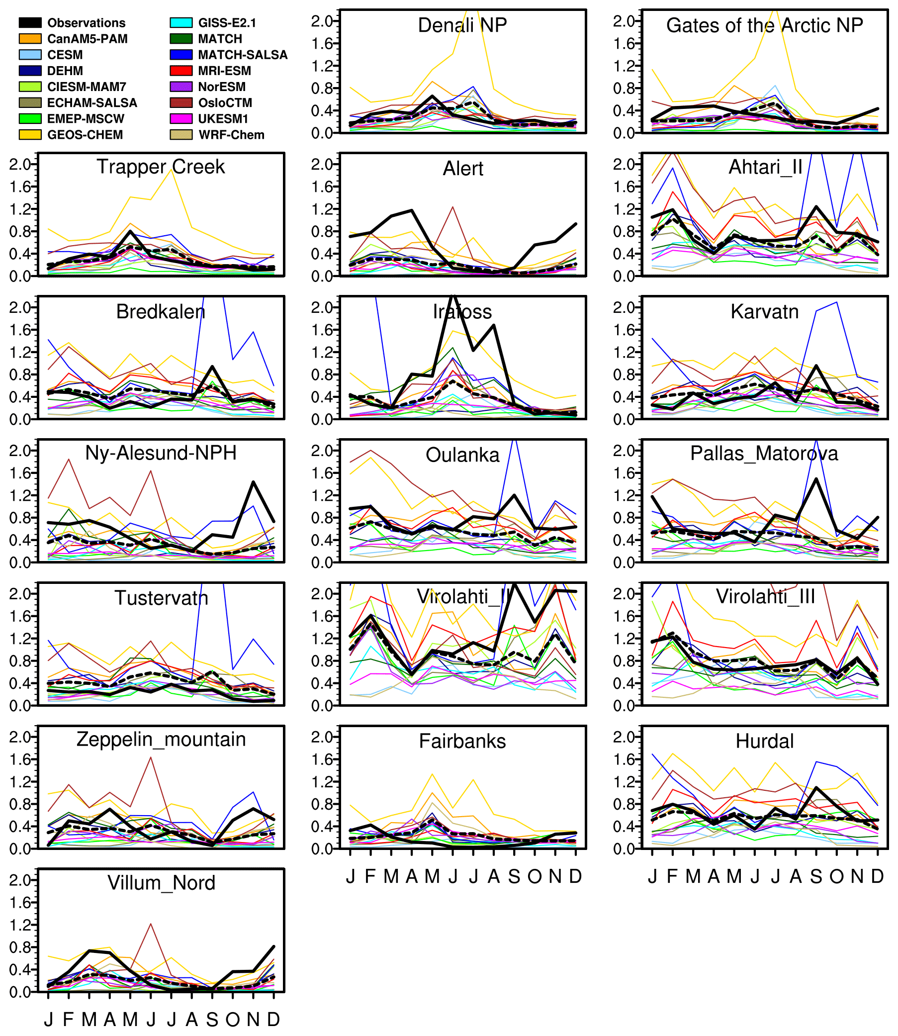
Figure 19Modeled (thin colored lines) and measured (thick black line) monthly mean SO concentrations (µg m−3) at surface Arctic measurement sites in 2014–2015. The multi-model mean is shown by the black dashed line.
The high GEOS-Chem bias in the summertime seen in Fig. 19 was first reported in Breider et al. (2014) and found to be due to problems with cloud pH and cloud liquid water in the summer over the Arctic. In Breider et al. (2017), the summertime Arctic surface SO concentrations are reduced by a factor of 2 by reducing the cloud liquid water content to a uniform value of 1 × 10⁻⁷ g m−3 north of 65∘ N in the model. The version of GEOS-Chem in our study is more recent and uses the offline cloud liquid water content from both GEOS-FP and MERRA2. We did not scale this variable down, which may be a reason for the high GEOS-Chem sulfate bias in Fig. 19.
The seasonal cycle for observations grouped together is shown in Fig. S10, showing a consistent seasonal cycle for 2008–2009 as seen in the observations. Most models (e.g., CanAM5-PAM, DEHM, MATCH, OsloCTM) are able to capture the seasonal cycle well. However, several models (e.g., CESM, CIESM-MAM7, ECHAM-SALSA, and EMEP-MSCW) strongly underestimate observed springtime peak values. Conversely, the models and the measurements showed a weaker seasonal cycle during the 2014–2015 time period (Fig. S11). It may be partly due to the local pollution sources in the Arctic during wintertime (e.g., Fairbanks). Those highly localized pollution events, caused by local emissions getting trapped in a stable boundary layer, occur on scales that are smaller than the model resolutions employed here can represent. Many models are also missing chemical formation processes for SO in the absence of sunlight, which may explain underestimations seen in winter (e.g., Moch et al., 2018; Alexander et al., 2009). An evaluation of SO2 could help with our understanding but was beyond the scope of this study. A lack of dark chemistry may be true for organic aerosol, as discussed in the next section as well.
From October to December 2014, the Honoluraun volcanic eruption may have elevated SO concentrations at some locations in the Arctic. However, in our model–measurement comparisons, there does not appear to be a large underestimate during those months, which implies that model performance was not impeded by not including those volcanic emissions.
As mentioned above, the uncertainty in wet deposition could be a significant factor in atmospheric SO model biases. Previous studies have shown that models have too much washout in winter and not enough wet deposition in summer, leading to a “flatter” seasonal cycle than observed (e.g., Fig. 19; Browse et al., 2012; Mahmood et al., 2016). As with BC in the previous section, the SO deposition was evaluated here in the same manner. The average measured SO deposition fluxes from ice cores for all locations (only Greenland was available here) are 18 mg m−2 yr−1. The lowest observed fluxes are found at D4 (12 mg m−2 yr−1) and the highest at ACT11D (30 mg m−2 yr−1). The model average for all locations is overestimated by around 20 % compared to measured fluxes. This is similar to the model biases in atmospheric SO concentrations.
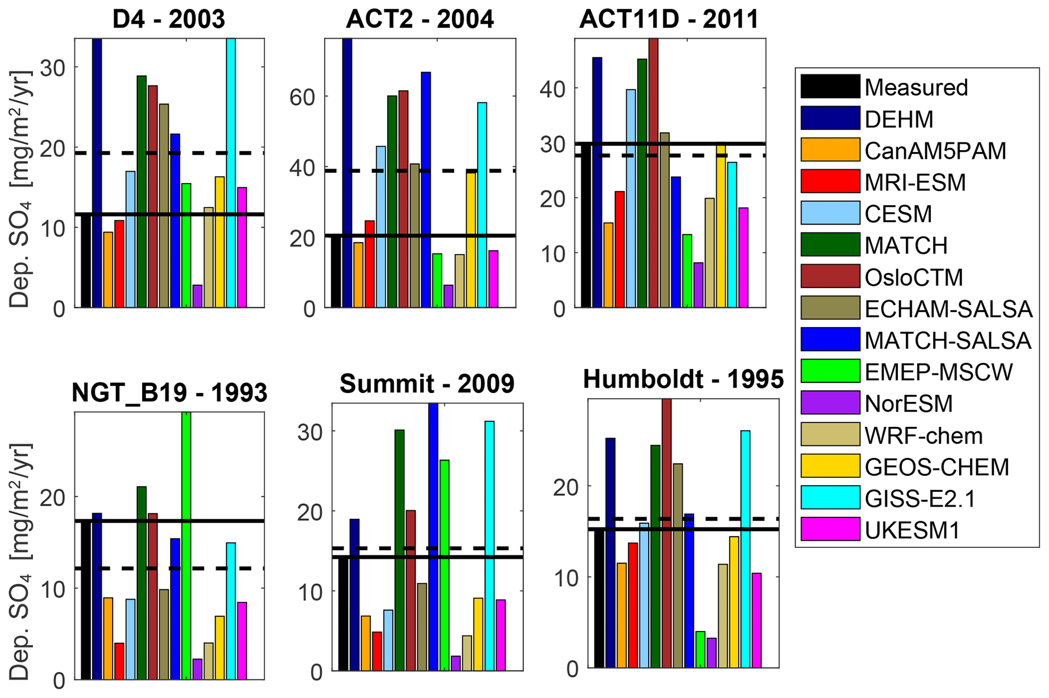
Figure 20SO deposition fluxes for the Greenland ice core locations shown in Fig. 1b. The observed fluxes are plotted in black, and a black line indicates the level of the average observed flux; the black dashed line is the multi-model mean at that location. The period used for plotting is based on all available years after 1990; the title indicates the last available year from the ice core record.
Therefore, the general model evaluation for SO indicates that while there is a large variability in models results, as with BC, models underestimate surface SO in the Arctic. The evaluation of SO deposition in the Arctic is similar to BC, with both overestimating deposition.
4.7 Organic aerosol
Unfortunately, there is only one high-Arctic station with OA measurements (Alert, NV, Canada); however, there are a few additional stations measuring OA in the sub-Arctic (still > 60∘ N). These are all shown in Fig. 21. The seasonal cycles are shown in Fig. 22, and the model vs. measurement scatter plot along with some comparison statistics are presented in Fig. S12.
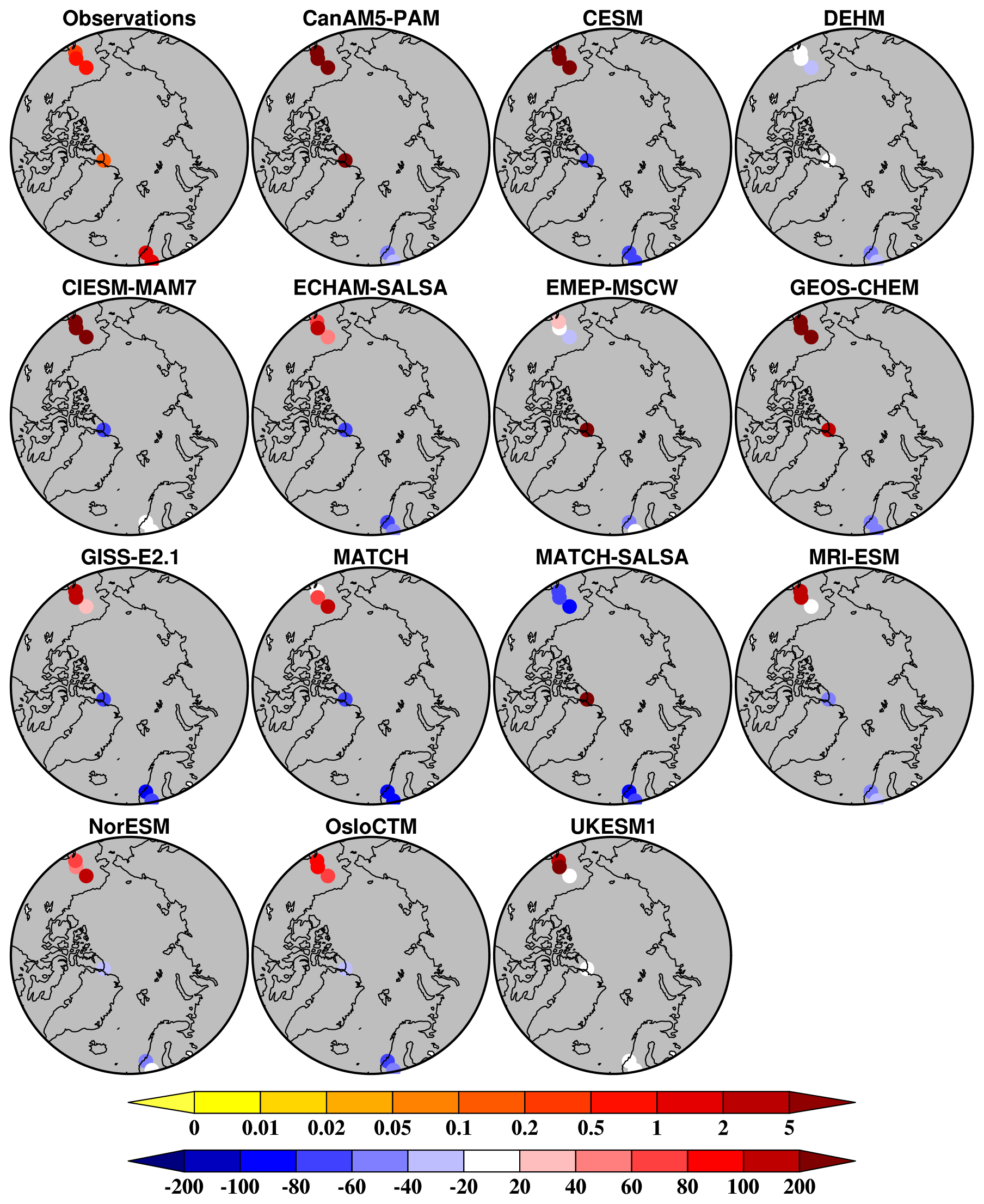
Figure 21Mean OA concentrations (µg m−3, top color bar) at surface Arctic measurement sites and model bias (as model–measurement measurement in percent, bottom color bar) for 2014–2015. Results from 2008–2009 are similar and not shown.
Model biases have a large range of ±200 % at the different locations, but the multi-model mean for the region is +65 %. At midlatitudes (30–60∘ N), measurements are conducted mainly in the US, where the multi-model mean bias is +83 % for the 2014–2015 average (not shown).
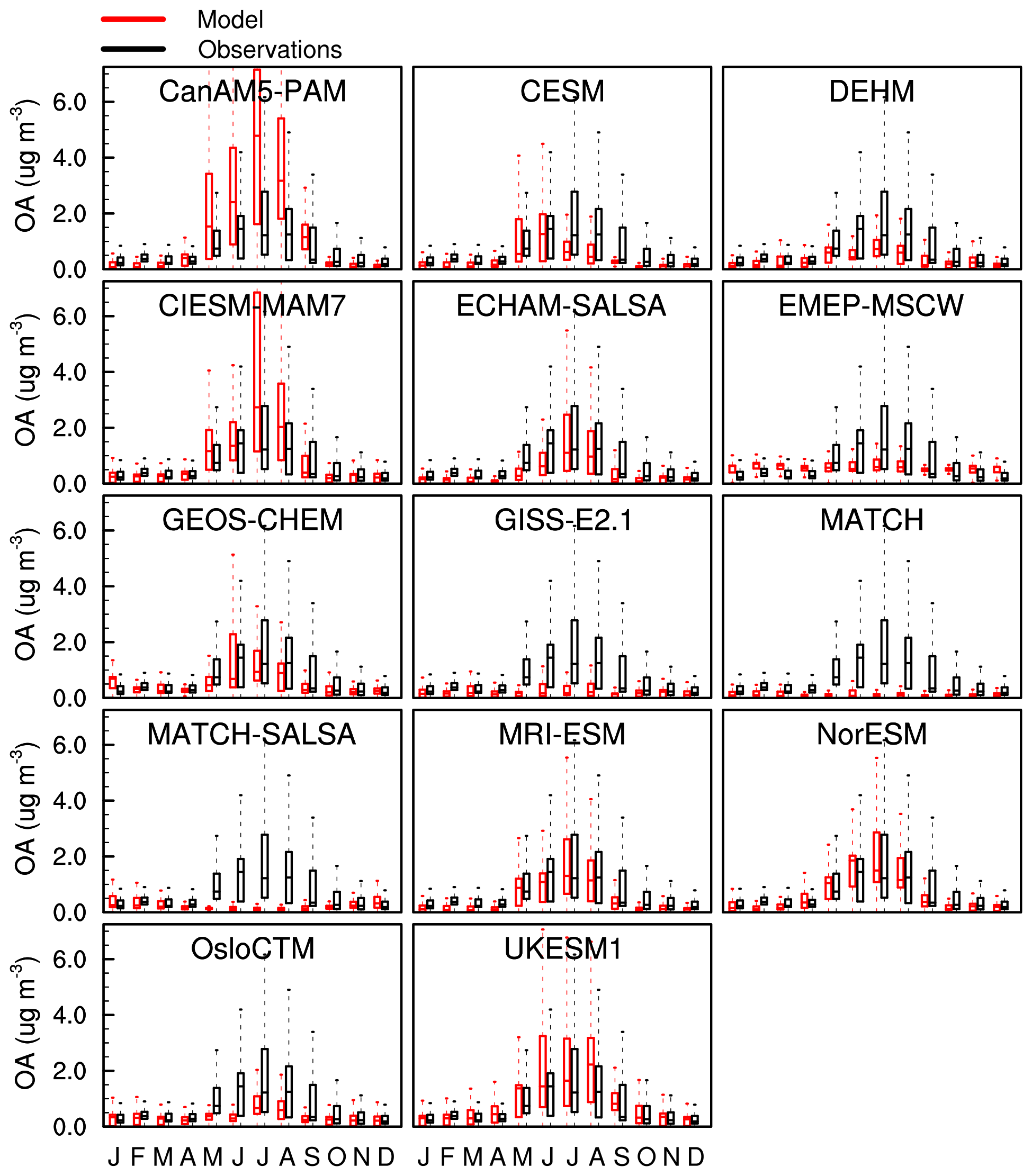
Several models (CanAM5-PAM, DEHM, CIESM-MAM7, ECHAM-SALSA, GEOS-Chem, MRI-ESM2, NorESM, OsloCTM, and UKESM1) are able to simulate the summertime peak in Arctic OA concentrations; however, the other seven models in Fig. 22 simulate a seasonal cycle that is too flat or peaks at the wrong time (e.g., the CESM seasonal cycle peaks too early in the year).
Figures 21 and S11 both show that most models consistently overestimate Alaskan OA and underestimate European OA, consistent with our assessment of other species showing that models are likely overestimating wildfire influence in summertime Alaska. All models, except EMEP-MSC-W, used the GFED fire emissions inventory. EMEP-MSC-W used the FINN fire emissions inventory, which for BC+OC has been shown to be significantly lower than the GFED emissions (Liu et al., 2020). As a result, EMEP-MSC-W model biases in Alaska are lower. However, they are not the lowest. MATCH-SALSA has the lowest OA model biases in Alaska, despite that model using GFED emissions. The comparison statistics in Fig. S12 show highly varying results.
4.8 Fine particulate matter
PM2.5 is partly connected to direct and indirect climate effects via its interactions with clouds. It is mainly composed of BC, SO, OA, NO, and NH, as well as crustal material (dust), sea salt, and water, though the water component is often dried off during measurements. Model biases of those species will contribute to the total PM2.5 biases.
While BC, SO, and OA were discussed above, it is beyond the scope of this project to evaluate the other major PM species, which, aside from water, have a smaller radiative impact. Note that the analysis in this section is focused on sub-Arctic and midlatitude sites closer to human populations rather than remote high-Arctic sites due to a lack of data. PM2.5 is not a typical parameter included in the longer-term remote Arctic observations. Since PM2.5 has important health impacts, it is well measured at air quality monitoring networks.
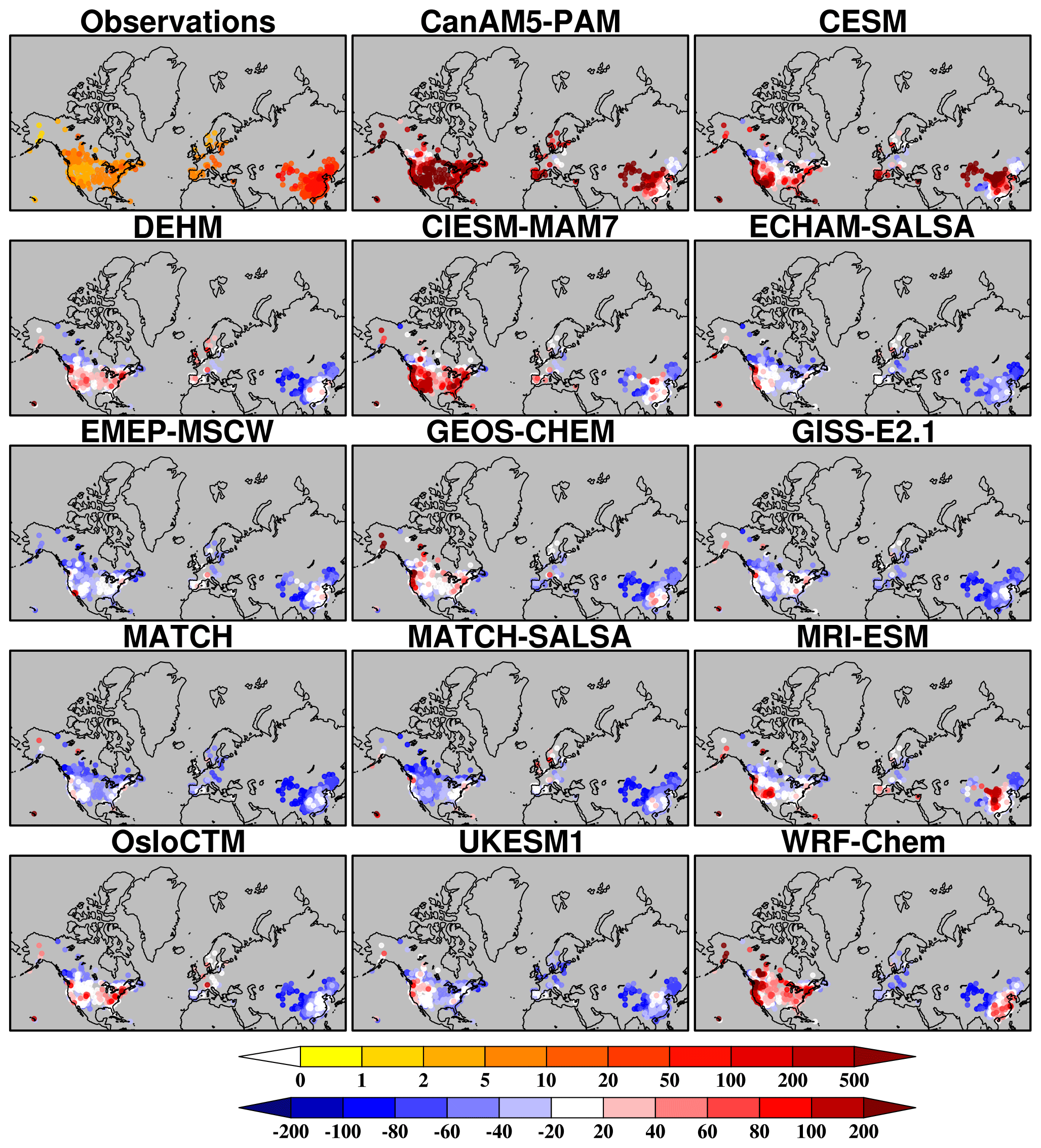
Figure 23Measured ground-level PM2.5 concentrations (µg m−3) and model biases (as model–measurement measurement in percent, bottom color bar) for 2014–2015. The upper color bar represents observations, and the lower bar represents model biases.
The model PM2.5 biases at several locations in the United States, Europe, and China are within the 60 %–80 % range. However, some models (CanAM5-PAM, CIESM-MAM7, GEOS-CHEM, GEM-MACH, and Oslo-CTM) show biases larger than 200 %, especially in the western US and Alaska. The large inter-model differences in Fig. 23 are likely due to uncertainty in mineral dust. CanAM5-PAM has a particularly large contribution of dust to PM2.5. The Turnock et al. (2020) study showed that dust regions were globally one of the largest areas of diversity in PM2.5 concentrations between different CMIP6 models. The EMEP MSC-W results are consistent with EMEP annual evaluations for Europe, where the model underestimates PM2.5 by 10 %–25 %, including a few Arctic sites in Norway and Finland (Gauss et al., 2020, and annual model evaluation reports at https://www.emep.int/publ/common_publications.html, last access: 14 April 2022).
The simulated surface-level SLCFs were quite sensitive to the different meteorological conditions such as boundary layer stability and levels of photochemistry, which differed between the two time periods chosen in this study. 2014–2015 was also a time period with more wildfires compared to 2008–2009. For example, according to the CMIP6 emission data that were used in most of the models, emissions of BC from Canadian wildfires in 2014–2015 were 340 % higher than in 2008–2009, whereas the emissions from the USA and Russia were similar for these years. Given the very intense wildfire emissions and low anthropogenic emissions in northern Canada in 2014–2015, differences in simulated PM2.5 concentrations over Canada and Alaska can be partly attributed to differences in simulations of wildfire aerosols in the models.
Some models (CanAM5-PAM, CESM, CIESM-MAM7, GEOS-Chem, and WRF-Chem) simulate higher PM2.5 and more variable PM2.5 in the summertime (e.g., Fig. S13 in the Supplement). While this is seen to some extent in the observations, this may be due to the way fire emissions and sea salt emissions are treated in these models. Fire emissions, fire plume injection height, plume rise, and wet deposition of fire pollutants are all highly uncertain model processes and a subject of ongoing research (e.g., Urbanski, 2014; Heilman et al., 2014; Paugam et al., 2016). Indeed, the individual model PM2.5 Arctic biases are more tightly clustered for 2008–2009 when there were fewer fires. Mölders and Kramm (2018) showed that Arctic PM2.5 seasonal pollution is mainly due to local air pollution in the winter and due to fires in the summer.

Figure 24Annual mean PM2.5 comparisons between station observations and model simulations for the year 2015.
Figure 24 shows that the annual mean simulated PM2.5 concentrations compare well with observations and the correlation coefficients are relatively high (R=0.8 or higher for all models). The high concentrations in China and low concentrations in the US and Europe are captured by the models, providing confidence for health impact assessments that utilize these model results.
In this study, we evaluated the SLCF simulation capabilities of 18 models that were used in the 2022 AMAP SLCF assessment report. Our conclusions are grouped into the questions we aimed to answer in the Introduction.
5.1 How well do the AMAP SLCF models perform in the context of measurements and their associated uncertainty?
Recall that the in situ SLCF measurements had the following reported uncertainties: CH4 1 %, O3 3 %, CO 5 %, NO2 5 %–100 %, BC 200 %, SO 20 %, OA 20 %, and PM2.5 1 %–6 %. However, since the variability in measurements from different techniques was only really taken into account for the BC uncertainty, and since we are comparing annual mean results to each other, it is not a fair comparison to say that models and measurements agree with each other if model biases are within the reported measurement uncertainty range. However, we do use those numbers as a rough guideline for “good” model performance in the absence of other quantitative criteria.
Some model annual mean biases were within those uncertainty ranges. For example, CMAM, MRI-ESM2, and UKESM1 simulate Arctic CH4 to within 1 %, thus agreeing with the CH4 measurements. However, at midlatitudes, they are all out of range at around +6 %–10 %. MATCH and WRF-Chem simulated midlatitude O3 to within 2 %, but only MATCH-SALSA was within 3 % in the Arctic region. The Arctic NO2 measurements are highly uncertain at around 100 %, so all of the models agreed with Arctic NO2 measurements. However, in the higher-NO2 midlatitude environment, NO2 measurement uncertainty is at the smaller end of the range. OsloCTM and WRF-Chem midlatitude NO2 biases were within 10 %. All models agree with BC measurements in both midlatitudes and the Arctic, as all biases are less than 80 %. CESM, CIESM-MAM7, DEHM, MATCH, UKESM1, and WRF-Chem all simulate midlatitude SO to within 20 %. But only CanAM5-PAM and MRI-ESM2 do the same for the Arctic region. OA had some of the largest model biases (Figs. 3 and 4), though ECHAM-SALSA, EMEP-MSC-W, GISS-E2.1, MATCH, and OsloCTM are all within 20 % in the Arctic but none at midlatitudes. Finally, with the small uncertainty in PM2.5, only CIESM-MAM7 in the midlatitudes and GISS-E2.1 in the Arctic agree within 2 %.
To summarize the mmm annual mean performance, it “matches” surface observations in the Arctic for CH4, NO2, BC, SO, OA, and PM2.5 – as such, the mmm has the best overall performance for the Arctic. In the midlatitudes the mmm matches surface observations for BC and SO only.
Regarding the comparisons of trace gases to the TES, MOPITT, and ACE-FTS satellite measurements (which have roughly 5 %–20 % uncertainty), models agree well. Free-tropospheric distributions of trace gases are somewhat easier to simulate, as common problems like a boundary layer that is too stable or too much deposition do not negatively impact the free-tropospheric SLCF distributions. The variability in the free troposphere is smaller compared to at the surface as well. It is also because of the previously noted difference between the spatial range that remote measurements cover being more akin to the spatial scale of model grid boxes compared to the point measurements from in situ observations.
5.1.1 What do the best-performing models have in common?
There were no models that performed best for all SLCF species and for all regions, highlighting the fact that it is difficult for any one model to bring together numerous complex processes and get results comparable to observations for all SLCFs. This would involve simulating aerosols and chemistry together with the right transport processes, meteorology, and clouds, which is difficult, especially for a remote region like the Arctic where parameterizations might have been built on datasets that are not always applicable there. In addition, studies like that of Tsigaridis et al. (2014) have shown that there was no clear change in model skill (in that case for OA) with increasing model complexity.
However, several models such as CanAM5-PAM, DEHM, NorESM, and MATCH have better representation of the vertical distribution of BC. DEHM and MATCH also had relatively small biases throughout the O3 tropospheric profile (CanAM5-PAM and NorESM did not simulate gas-phase SLCFs). MATCH in particular has the smallest surface O3 bias at midlatitudes, which may be related to its high vertical resolution in the boundary layer (the lowest two layers are 20 m thick and the four lowest layers are below 150 m). These models are a mix of air quality and climate-focused models; thus, it is important to note that there is no obvious difference between climate and air quality model biases for annual mean SLCFs. Despite the lack of complex tropospheric chemistry, CMAM had some of the lowest O3 biases at both midlatitudes and the Arctic. This may imply that the more complex chemistry is not needed in the context of climatological tropospheric O3 for climate studies (though of course, O3 on shorter timescales would need more complete tropospheric O3 chemistry). In the lower stratosphere, however, models with simplified or climatological O3 schemes did not perform as well as models that had full stratospheric chemistry included.
5.1.2 Are there regional patterns in the model biases?
Generally speaking, when comparing the midlatitude model biases to those of the Arctic, they skew more negative (Fig. 4), implying a lack of long-range transport to the Arctic. The best Arctic results for BC throughout the tropospheric profile were from models (CanAM5-PAM, DEHM, MATCH, WRF-Chem) that simulated the vertical mixing of BC well at midlatitudes. The first three of the four models were nudged to the ERA-Interim analysis, and WRF-Chem was nudged to the NCEP FNL analysis. The Arnold et al. (2015) study showed that a key determinant in model differences for peroxyacetyl nitrate (PAN) export relative to CO was the meteorology used in the models. Their results implied that the ERA-Interim models had more efficient vertical transport and mixing in midlatitude source regions compared to GEOS-driven models. In the current study, Arctic BC was greatly underestimated throughout the Arctic profile by MATCH-SALSA, EMEP MSC-W, and GEM-MACH, which had BC concentrations at midlatitudes dropping much too low in the free troposphere. Those models had different sources of meteorology (Table 2), and some may have insufficient convection schemes. For example, GEM-MACH is missing subgrid-scale deep and shallow convection, which is important for the exchange between the planetary boundary layer and free troposphere and consequently for transport at middle and high latitudes. This subject could be studied further via sensitivity tests with and without nudged meteorology, while keeping the aerosol physics the same.
The summertime evaluations of surface O3, BC, and OA all imply that models overestimate the amount of these pollutants coming from wildfires in the western Arctic. This could be due to uncertainties in wildfire emissions, fire plume transport, or, in the case of O3 and secondary OA, the plume chemistry. It is also likely that wet deposition of fire pollutants is underestimated if fire aerosol size is too small and due to climate models lacking pyrocumulus clouds and precipitation. The model overestimations of SLCFs in the summer could be due to a combination of all of these uncertainties.
Our analysis from ACE-FTS, TES, and the aircraft datasets show that CH4, O3, and BC model biases all imply that the modeled tropopause height is likely too low. Tropospheric species like CH4 and BC should drop rapidly above the tropopause, but model biases increase sharply at that point. Stratospheric species like O3 should increase rapidly above the tropopause, but model biases decline sharply there.
5.1.3 Are there patterns in the model biases between SLCF species?
Some patterns one might expect between SLCF species were not demonstrated in this study's results. For example, both O3 precursors, CO and NO2, are too low in models, though that underestimation is worse in the winter. Despite that, surface O3 tends to be overestimated, though that overestimation is mainly in the summer. Also, the west–east pattern in Arctic surface O3 was overestimated in Alaska and underestimated in Scandinavia. However, for CO and NO2 those skewed biases are reversed.
At midlatitudes SO, BC, and OA are biased high in most models, yet despite that, PM2.5 is underestimated. Thus, the PM2.5 biases must be significantly influenced by the other, mainly natural, aerosol components.
In addition to expected patterns, there were no other discernible patterns in model biases between SLCF species.
5.2 How does the model performance impact model applications, such as simulated climate and health impacts?
In the AMAP (2022) report, these models go on to be used to simulate future emission scenarios, and from those results, the future temperature changes due to these SLCFs are predicted. They are further used to determine future changes to human health due to the changes in SLCFs. Given the model evaluation of this study, we have determined that using the mmm to predict SLCF climate impacts is generally robust. Considering the SLCFs with the greatest radiative impact (CH4, O3, BC, and SO4), the mmm was within ±25 % of the measurements across the Northern Hemisphere. The mmm also performed very well for PM2.5, which is a main component considered for human health impacts. Thus, for climate studies, wherein relatively large regions and time periods are considered, the model performance is sufficient.
5.3 What processes should be improved or studied further for better model performance?
The model evaluation in this study brought about results that have been reported in previous publications, and several notable issues remain. Here we recommend some future work that may help improve model performance.
-
Models simulate too much surface O3 at midlatitudes, and this may be due inadequate treatment of dry deposition (Val Martin et al., 2014) and/or not including parameterizations for the shade provided by vegetation that reduces photochemistry, as reported in Makar et al. (2018). That said, MATCH had the smallest midlatitude surface O3 bias without accounting for canopy shading; hence, precursor emissions, vertical mixing, deposition, and O3 chemistry all have a role in model O3 results, and errors in these may sometimes cancel out.
-
There are a number of indications that simulated boundary layers are too stable (not enough vertical lifting of SLCFs, too much O3 titration, too much BC and SO4 deposition). Therefore, increased convection at midlatitudes may be needed. However, this hypothesis is opposite to that found in Allen and Landuyt (2014), which found that excessive tropical convection caused CMIP5 models to overestimate BC aloft. It is therefore important to evaluate models specifically for export and long-range transport events driven by different mechanisms (e.g., frontal export, convective lifting), which is a focus within the PACES initiative (Arnold et al., 2016).
-
The O3, BC, and PM2.5 model biases were all high in the Alaskan summertime, implying that many models may simulate too much pollution from wildfires there. Models need improved wildfire parameters for emissions, plume height, plume chemistry, and aerosol–cloud processes. For example, the fire emissions inventories GFED4, GFASv1.2, and FINNv1.5 vary by up to a factor of 3 for BC emissions (AMAP, 2022); light and temperature attenuation under smoke plumes means less O3 is produced than precursor concentrations may imply, and plume rise and injection height need to be accurate for long-range transport.
-
Modeled deposition is highly uncertain, and there is evidence here that some models have too much deposition of BC at midlatitudes. However, deposition measurements are scarce, even at midlatitudes, and more of those measurements are needed to constrain models.
-
Additional, preferably long-term, OA and PM2.5 measurements are needed in the high Arctic. Both are expected to be important to Arctic conditions in the future, with increasing wildfires and shipping influencing the Arctic atmosphere, and the lack of those measurements is problematic for constraining models.
-
An evaluation of SO2 would help to determine if the model biases in SO are due to transport, emission uncertainty, or if it can be explained by the uncertainty in chemistry. The removal of particles represents a large uncertainty, but without SO2 (and DMS) it cannot be concluded that the removal is too fast.
Therefore, we conclude that sensitivity tests for the abovementioned model processes will be important for further understanding and improving model performance for SLCFs. But just as important is having additional Arctic measurements and the continuation of existing Arctic measurements in order to assess the model improvements.
The 18 models used in this study are described in each subsection below. Table A1 contains further information summarizing the models' setup for the AMAP SLCF simulations.
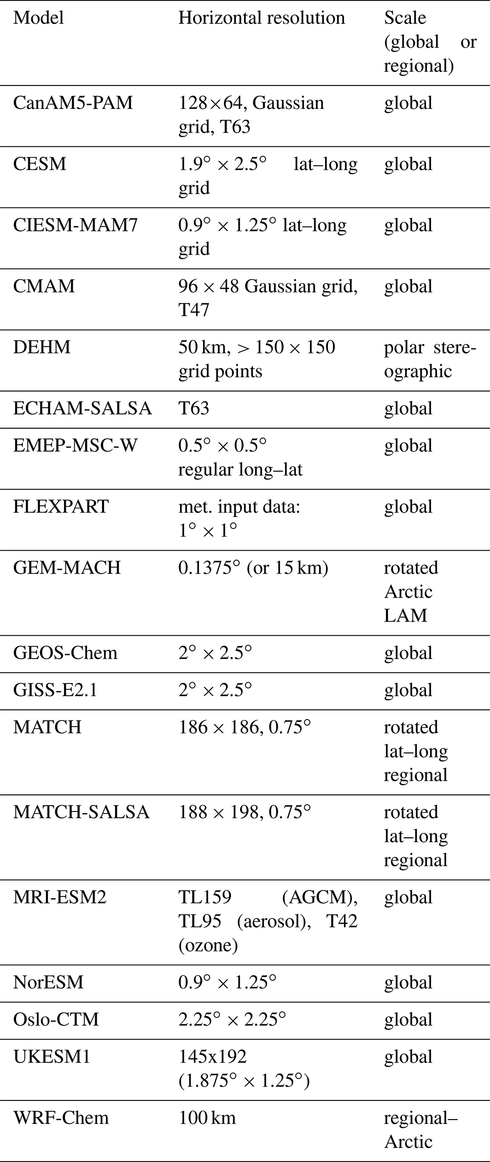
A1 CanAM5-PAM
The Canadian Atmospheric Model version 5 (CanAM5), with the Piecewise lognormal approximation Aerosol Model (PAM), was used. CanAM5-PAM is an improved version of CanAM4 (von Salzen et al., 2013). The improvements include a higher vertical resolution, improved parameterizations for land surface and snow processes, DMS emissions, and clear-sky radiative transfer. CanAM5-PAM has 49 vertical levels extending up to 1 hPa with a resolution of approximately 100 m near the surface. Model simulations are performed using a spectral resolution of T63, which is equivalent to the horizontal resolution of approximately 2.8∘ × 2.8∘. The model uses separate parameterizations for layer and convective clouds. Aerosol microphysical processes are based on the piecewise lognormal approximation (von Salzen, 2006; Ma et al., 2008; Peng et al., 2012; Mahmood et al., 2016, 2019; AMAP, 2015a). The model simulates binary homogeneous nucleation of sulfuric acid and water vapor. Newly formed particles grow by condensation and coagulation.
A detailed description of parameterizations of ocean DMS flux to atmosphere, oxidation, and removal processes is provided in Tesdal et al. (2016). In-cloud production of sulfate requires O3 and hydrogen peroxide (H2O2) as oxidants (von Salzen et al., 2000), with oxidant (OH, NO, H2O2, O3) concentrations specified as climatological results from CMAM. Dry deposition of aerosol depends on concentrations of aerosols in the near-surface model layer (Zhang et al., 2001). Wet deposition includes in-cloud scavenging in both convective clouds and layer clouds, as well as below-cloud scavenging.
Cloud droplet number concentrations are calculated based on the assumption of a parcel of air which ascends from the subcloud layer into the cloud layer with a characteristic vertical velocity (Peng et al., 2005); the standard deviation of the subgrid-scale cloud vertical velocity probability distribution is parameterized using the approach by Ghan et al. (1997). Aerosol particles that are suspended in the parcel of air may activate and grow into cloud droplets by condensation of water vapor. A numerically efficient solution of the condensational droplet growth equation (e.g., Seinfeld and Pandis (2006)) is employed for this purpose. In grid cells that are affected by clouds, CanAM5-PAM accounts for cloud albedo and lifetime effects (first and second aerosol indirect effects) as well as semi-direct effects.
A2 CESM
The Community Earth System Model version 2 (Danabasoglu et al., 2020) is an ESM that can be configured in many different ways. The configuration applied for this assessment utilized the Community Atmosphere Model (CAM) version 6 and Modal Aerosol Model (MAM4) with four mixed-species aerosol modes (Liu et al., 2016). CAM6 employs a spectral element dynamical core (Lauritzen et al., 2018). Type 0 and Type 1 CESM runs were conducted at 1.9∘ × 2.5∘ horizontal resolution, while Type 3 runs were conducted at 0.9∘ × 1.25∘, all with 32 vertical layers. For Type 0 and Type 1 simulations, CESM version 2.0 was used with CAM6-chem representations of chemical reactions (Emmons et al., 2020b), enabling prognostic simulation of tropospheric ozone concentrations, along with a volatility basis set (VBS) parameterization for the formation of secondary organic aerosol (SOA) (Tilmes et al., 2019) and stratospheric chemistry. CAM6-chem is coupled to the interactive Community Land Model (CLM5), which provides biogenic emissions, calculated online using the MEGANv2.1 algorithm (Guenther et al., 2012), and handles dry deposition. Tracked aerosol species simulated by MAM4 include sulfate, primary and aged black carbon and organic matter, dust, sea salt, and secondary organic aerosols. Both sea salt and dust emissions are calculated on-line and are highly sensitive to the surface wind speed (Mahowald et al., 2006a, b). These runs were also forced with prescribed sea surface temperatures (SSTs) and sea ice concentrations, created from merged Reynolds–HADISST products as in Hurrell et al. (2008). Type 3 transient runs utilized CESM version 2.1.1 without atmospheric chemistry and with fully coupled atmosphere, ocean, land, and sea ice components (component set BSSP245cmip6), as applied to simulate future scenarios for CMIP6. All CESM runs specified global mean mixing ratios of methane and carbon dioxide.
A3 CIESM-MAM7
CIESM-MAM7 is the Community Integrated Earth System Model (CIESM) (Lin et al., 2020) using the Modal Aerosol Model (MAM7) with seven mixed-species aerosol modes (Liu et al., 2012). The current CIESM version 1.1 (see Table 1 of Lin et al., 2020) is based on the NCAR Community Earth System Model (CESM version 1.2.1) with several novel developments and modifications aiming to overcome some persistent systematic biases, such as the double Intertropical Convergence Zone (ITCZ) problem and underestimated marine boundary layer clouds. CIESM-MAM7 employs a finite-volume dynamical core with 0.9∘ × 1.25∘ for horizontal resolution and 31 layers for vertical resolution. The large-scale meteorology (horizontal wind field) is nudged towards ERA-Interim reanalysis data and the relaxation time is set to 6 h. In CIESM-MAM7, the primary emissions of black carbon (BC), organic carbon (OC), ammonia (NH3), volatile organic compounds (VOCs), sulfur dioxide (SO2), and oxidizing gases (H2O2, O3, OH) are prescribed by the input data uniformly provided by the AMAP-SLCF group. The emission amounts of dust (DU) and sea salt (SS) are calculated online. Aerosol size distributions in CIESM-MAM7 are described by the seven overlapping lognormal distributions, including Aitken, accumulation, primary carbon, fine dust and sea salt, coarse dust, and sea salt modes. The geometric standard deviation of each mode is prescribed (see Table 1 of Liu et al., 2012). A simplified gas- and liquid-phase chemistry is included in CIESM-MAM7. SO2 and dimethyl sulfate (DMS) can be oxidized to sulfuric acid gas (H2SO) and then condenses to form the sulfate aerosols, while the evolution of oxidizing gases is not considered. Primary organic matter (POM) and BC are emitted to the primary carbon mode, then aged and transferred to the accumulation mode by condensation of H2SO, NH3, and semi-volatile organics and by coagulation with Aitken and accumulation modes. The effect of stratospheric sulfate aerosol from volcanic emission on radiative forcing is considered by following the CMIP6 procedure (Thomason, 2012). No specific stratospheric chemistry is included in CIESM-MAM7.
A4 CMAM
The Canadian Middle Atmosphere Model (CMAM) is based on the third-generation CanAM model, with the model lid raised to approximately 95 km and the necessary radiative processes for the mesosphere included (Scinocca et al., 2008). A representation of gas-phase chemistry has also been included that contains a relatively complete description of the HOx, NOx, Clx, and Brx chemistry that controls stratospheric ozone along with the longer-lived source gases such as CH4, N2O, and CFCs (Jonsson et al., 2004). For the troposphere the chemical mechanism can considered as methane–NOx chemistry as it does not include the chemistry of larger volatile organic compounds. The model does, however, include a description of associated tropospheric chemical processes such as wet and dry deposition, interactive NOx emissions from lightning, corrections of clear-sky photolysis rates for clouds, and N2O5 hydrolysis on prescribed sulfate aerosol distribution using the reaction probabilities of Davis et al. (2008). The simulation analyzed here used a “specified dynamics” setup, wherein the model horizontal winds and temperature are nudged towards a meteorological reanalysis dataset that represents the observed historical evolution of the atmosphere. In this way the day-to-day variability of the model meteorology is much more closely aligned with the historical evolution of the atmosphere than would be possible in a free-running model. Here CMAM was nudged to 6-hourly fields from the ERA-Interim reanalysis (Dee et al., 2011) on all model levels below 1 hPa and with a relaxation time constant of 24 h.
A5 DEHM
The Danish Eulerian Hemispheric Model (DEHM) (Christensen, 1997; Brandt et al., 2012; Massling et al., 2015) is a 3-D Eulerian atmospheric chemistry transport model developed at the Department of Environmental Science at Aarhus University in Denmark. The model domain covers the Northern Hemisphere using a polar stereographic projection with a grid resolution of 150 km × 150 km. It includes nesting capabilities to make simulations with a higher grid resolution in a limited area of the domain, and in this work an Arctic sub-domain with 50 km × 50 km has been applied covering the Arctic area down to about 40–54∘ N. The model has 29 vertical levels in sigma coordinates; the lowest 15 levels are below 2000 m above the surface. The lowest model levels are 22 m thick, and the top of the model domain is at 100 hPa, i.e., the whole troposphere and very lowest part of the stratosphere. DEHM includes a SOx–NOx–VOC–ozone chemistry, with 71 components including secondary organic aerosol (SOA), the use of the VBS mechanism, and nine particulates including hydrophobic and hydroscopic BC, primary organic aerosols, primary anthropogenic dust, PM2.5 fraction, and coarse fraction of PM10 of sea salt and Pb. CH4 is a prognostic species for which the boundary conditions have a large influence. The model is driven by meteorological data from a numerical weather prediction model from the WRF model (Skamarock et al., 2008) version 3.9, with 1 h resolution. The WRF model system is driven by reanalysis data from the ERA-Interim made by ECMWF by nudging.
A6 ECHAM-SALSA
ECHAM-SALSA is the general aerosol–climate model ECHAM-HAMMOZ (ECHAM6.3-HAM2.3-MOZ1.0) (Tegen et al., 2019; Schultz et al., 2018) using the Sectional Aerosol module for Large Scale Applications (SALSA) (Kokkola et al., 2018) to solve the aerosol microphysics. ECHAM6 (Stevens et al., 2013) computes the atmospheric circulation and fluxes using a semi-Lagrangian transport scheme. In the setup used here, the large-scale meteorology (vorticity, divergence, and surface pressure; relaxation times of 24, 6, and 48 h, respectively) was nudged towards ERA-Interim reanalysis data (Berrisford et al., 2011). In SALSA the aerosol size distribution is modeled using 10 size sections (or bins), which span particle sizes between 3 nm and 10 µm. The size distribution is further divided into a soluble and an insoluble sub-population, which are treated as externally mixed. Within one size bin of one sub-population, all aerosol particles are considered internally mixed. In its standard setup, SALSA describes the aerosol compounds, BC, organic carbon (OC), SO, SS, and mineral dust (DU). In the model, BC, OC, SS, and DU are emitted as primary particles, while SO is emitted as either SO2 or as DMS, which are oxidized using a simplified chemistry (Stier et al., 2005) to form H2SO4, which then either nucleates or condenses onto existing particles. BC, OC, and SO2 emissions are prescribed using input files, while SS and DU emissions are computed online. All greenhouse gas concentrations are fixed to pre-defined concentrations. The model resolution for the simulations performed here was T63 (roughly 2∘ by 2∘), further using 47 hybrid sigma-pressure levels.
A7 EMEP MSC-W
The EMEP MSC-W model is a 3-D Eulerian chemistry transport model developed at the Norwegian Meteorological Institute within the framework of the UN Convention on Long-range Transboundary Air Pollution. It is described in detail in Simpson et al. (2012). Although the model has traditionally been aimed at simulations of acidification, eutrophication, and air quality over Europe, global modeling has been performed and evaluated against observations for many years (Jonson et al., 2010; Wild et al., 2012). The model uses 20 vertical levels defined as eta-hybrid coordinates. The 10 lowest levels are within the planetary boundary layer (with the bottom layer being 92 m thick), and the top of the model domain is at 100 hPa. Model updates since Simpson et al. (2012), resulting in EMEP model version rv4.33 as used here, have been described in Simpson et al. (2019) and references cited therein. The main revisions were made to the parameterizations of coarse NO formation on sea salt and dust aerosols, N2O5 hydrolysis on aerosols, and additional gas–aerosol loss processes for O3, HNO, and HO2. The EMEP model, including a user guide, is publicly available as open-source code at https://github.com/metno/emep-ctm (last access: 14 April 2022). EMEP-modeled PM2.5 and PM10 include primary and secondary aerosols, both anthropogenic and natural. Secondary aerosol consists of inorganic sulfate, nitrate, ammonium, and SOA; the latter is formed from both anthropogenic and biogenic emissions using the VBS scheme detailed in Bergström et al. (2012) and Simpson et al. (2012). The model also calculates sea salt aerosols and windblown dust particles from soil erosion. Aerosol optical depth (AOD) is calculated based on the mass concentrations of individual aerosols multiplied by corresponding mass extinction coefficients. In these simulations, we did not use the BC and OC emissions from EclipseV6b directly, but applied EclipseV6b PM2.5 and coarse PM emissions instead, which were split into elementary carbon (EC), organic matter (OM) (here assumed inert), and the remaining inorganic dust. The EC and OM emissions in the fine and coarse fractions were further divided into fossil fuel and wood-burning compounds for each country and source sector. The split applied to the PM emissions is the same as used in EMEP operational runs (IIASA, personal communication). A total of 80 % of emitted EC is assumed to be hydrophobic, aging to become hydrophilic within 1 to 1.5 d. As in Bergström et al. (2012), the organic matter to organic carbon ratio of emissions by mass is assumed to be 1.3 for fossil fuel sources and 1.7 for wood-burning sources. Note that different wildfire emissions were used here, i.e., from FINN (the Fire INventory from NCAR version 15). The EMEP model runs were driven by 3-hourly meteorological data from the ECMWF IFS model at 0.5∘ × 0.5∘ resolution.
A8 FLEXPART
The Lagrangian particle dispersion model FLEXPART version 10.4 (Pisso et al., 2019) releases computational particles that are simulated forward in time following 3-hourly ECMWF meteorological fields with 137 vertical layers and a spatial resolution of 1∘ × 1∘. For each year around 330 million particles were released to calculate turbulent diffusion (Cassiani et al., 2014), unresolved mesoscale motions (Stohl et al., 2005), and convection (Forster et al., 2007). A recently updated wet deposition scheme taking into account in-cloud and below-cloud removal was used (Grythe et al., 2017). Gravitational settling for spherical BC particles with an aerosol mean diameter of 0.25 µm, a normalized standard deviation of 3.3, and a particle density of 1500 kg m−3 (Long et al., 2013) is used in the calculation of dry deposition. The surface concentration and deposition fields were retrieved on a monthly basis on a resolution of 0.5∘ × 0.5∘.
A9 GEM-MACH
GEM-MACH (Global Environmental Multiscale model–Modelling Air quality and CHemistry) is the Environment and Climate Change Canada (ECCC) air quality prediction model. It consists of an online tropospheric chemistry module embedded within ECCC's GEM numerical weather forecast model (Côté et al., 1998b, a; Charron et al., 2012). The chemistry module includes a comprehensive representation of air quality processes, such as gas-phase, aqueous-phase, and heterogeneous chemistry and aerosol processes (e.g., Moran et al., 2018; Makar et al., 2015b, a; Gong et al., 2015). Specifically, gas-phase chemistry is represented by a modified ADOM-II mechanism with 47 species and 114 reactions (Lurmann et al., 1986); inorganic heterogeneous chemistry is parameterized by a modified version of the ISORROPIA algorithm of Nenes et al. (1999), as described in detail in Makar et al. (2003); SOA formation is parameterized using a two-product, overall, or instantaneous aerosol yield formation (Odum et al., 1996; Jiang, 2003; Stroud et al., 2018); aerosol microphysical processes, including nucleation and condensation (sulfate and SOA), hygroscopic growth, coagulation, and dry deposition and sedimentation, are parameterized as in Gong et al. (2003); the representation of cloud processing of gases and aerosols includes uptake and activation, aqueous-phase chemistry, and wet removal (Gong et al., 2006, 2015).
Aerosol chemical composition is represented by eight components: sulfate, nitrate, ammonium, elemental carbon (EC), primary organic aerosol (POA), secondary organic aerosol (SOA), crustal material (CM), and sea salt; aerosol particles are assumed to be internally mixed. A sectional approach is used for representing aerosol size distribution. For the 2015 Arctic simulation, a 12-bin (between 0.01 and 40.96 µm in diameter, logarithmically spaced: 0.01–0.02, 0.02–0.04, 0.04–0.08, 0.08–0.16, 0.16–0.32, 0.32–0.64, 0.64–1.28, 1.28–2.56, 2.56–5.12, 5.12–10.24, 10.24–20.48, and 20.48–40.96 µm) configuration is used.
The Type 0 simulation was conducted for the year 2015 over a limited-area model (LAM) domain on a rotated lat–long grid at 0.1375∘ × 0.1375∘ (or 15 km) resolution covering the Arctic (> 60∘ N) and extending to the southern US–Canada border. Some of the model upgrades for the Arctic simulation are described in Gong et al. (2018). Anthropogenic emissions used are based on a combination of North American emission inventories (specifically, the 2016 US National Emission Inventories and 2015 Canadian national Air Pollution Emission Inventories) and global ECLIPSE v6b 2015 baseline emissions. North American wildfire emissions are processed using the Canadian Forest Fire Emission Prediction System (CFFEPS) from satellite-detected fire hotspot data (MODIS, AVHRR, and VIIRS). CFFEPS consists of a fire growth model, a fire emissions model, and a thermodynamic-based model to predict the vertical penetration height of a smoke plume from fire energy (see Chen et al., 2019, for details). Biogenic emissions are calculated online in GEM-MACH based on the algorithm from BEIS version 3.09 with BELD3-format vegetation land cover. Sea salt emissions are computed based on Gong et al. (2003).
The chemical lateral boundary conditions were from MOZART-4/GEOS-5 (Emmons et al., 2010). The meteorology was initialized daily (at 00:00 UTC) using the Canadian Meteorological Centre's global objective analyses.
A10 GEOS-Chem
GEOS-Chem is a global three-dimensional chemical transport model driven by assimilated meteorological observation from the Goddard Earth Observing System (GEOS) of the NASA Data Assimilation Office (DAO), which was first introduced in 2001 (Bey et al., 2001). GEOS-Chem is a grid-independent model which operates on a 1-D column with default or user-specified horizontal grid points, vertical grid points, and time step. GEOS-Chem Classic can use archived GEOS meteorological data on a rectilinear latitude–longitude grid to compute horizontal and vertical transport and use Open-MP in parallelization. Two types of assimilated meteorological data from the NASA Global Modeling and Assimilation Office (GMAO) can be used to drive the offline mode of GEOS-Chem. The first type are operational data starting from 2012, the GEOS Forward Processing (GEOS-FP, the native resolution of which was 0.25∘ × 0.3125∘; Lucchesi, 2013). The second type is the consistent Modern-Era Retrospective Analysis for Research and Applications version 2 (MERRA-2, starting from 1979–present; Randles et al., 2017), with the native resolution 0.5∘ × 0.625∘. Both types of meteorological data have 72 hybrid sigma-pressure levels with the top at 0.01 hPa, 3-hourly temporal resolution for 3-D fields, and 1 h resolution for 2-D fields. The advection scheme of GEOS-Chem uses the TPCORE advection scheme (Lin and Rood, 1996) on the latitude–longitude grid, while the convective transport uses the convective mass flux described by Wu et al. (2007). The wet deposition scheme in GEOS-Chem is based on Liu et al. (2001) for water-soluble aerosols and Amos et al. (2012) for gases. The dry deposition is based on the resistance-in-series scheme of Wesely (1989). Aerosol deposition is from Zhang et al. (2001). Emissions of dust aerosol, lightning NOx, biogenic VOCs, soil NOx, and sea salt aerosol are dependent on the local meteorological conditions. The CEDS global inventory provides the default anthropogenic emissions, while EDGAR v4.3.2 (M. et al., 2018) is also available as an alternate option to CEDS. Future anthropogenic emissions following the RCP scenarios (, ), aircraft emissions (Stettler et al., 2011), ships emission (from CEDS), and lighting NOx emissions (Murray et al., 2012) are also included and configured at run time using the HEMCO module described (Keller et al., 2014). Biogenic VOC emissions in GEOS-Chem are from the MEGAN v2.1 inventory (Guenther et al., 2012). The chemical solver in the standard GEOS-Chem simulation uses the Kinetic PreProcessor (KPP) (Damian et al., 2002) as implemented in GEOS-Chem. The gas phase in the troposphere in GEOS-Chem includes a detailed HOx–NOx–VOC–ozone–halogen–aerosol tropospheric chemistry mechanism, which generally follows JPL/IUPAC recommendations including PAN (Fischer et al., 2014), isoprene (Travis et al., 2016; Fisher et al., 2016), halogens (Sherwen et al., 2016; Chen et al., 2017), and Criegees (Millet et al., 2015). A linearized stratospheric chemistry scheme has been implemented since GEOS-Chem v9.0. The model will read from archived 3-D monthly mean production rates and losing frequency for each species at the beginning of each month. The Linoz chemistry (McLinden et al., 2000) is also applied as a recommended option for the stratospheric ozone layer. The original sulfate–nitrate–ammonium aerosol simulation in GEOS-Chem coupled to gas-phase chemistry (Park et al., 2004). The black carbon simulation (Wang et al., 2014), organic aerosol (Pai et al., 2020), complex SOA (Pye et al., 2010), the aqueous-phase isoprene SOA scheme (Marais et al., 2016), and the dust simulation (Duncan Fairlie et al., 2007) are also implemented into GEOS-Chem. The dust size distributions are from Zhang et al. (2013). GEOS-Chem v12.3.2 with uniform 2∘ × 2.5∘ MERRA-2 meteorological data for 2008–2009, GEOS-FP meteorological data for 2014–2015, and ECLIPSEv6b emissions was used in this study.
A11 GISS-E2.1
The NASA Goddard Institute of Space Studies (GISS) Earth system model (ESM), GISS-E2.1, is a fully coupled ESM. A full description of GISS-E2.1 as well as evaluation of its coupled climatology during the satellite era (1979–2014) and the historical ensemble simulation of the atmosphere and ocean component models (1850–2014) are described in Kelley et al. (2020). GISS-E2.1 has a horizontal resolution of 2∘ in latitude by 2.5∘ in longitude and 40 vertical layers extending from the surface to 0.1 hPa in the lower mesosphere. The tropospheric chemistry scheme used in GISS-E2.1 (Shindell et al., 2001, 2003) includes inorganic chemistry of Ox, NOx, HOx, CO, and organic chemistry of CH4 and higher hydrocarbons using the CBM4 scheme (Gery et al., 1989), as well as the stratospheric chemistry scheme (Shindell et al., 2006), which includes chlorine and bromine chemistry together with polar stratospheric clouds. The meteorology was nudged to the NCEP reanalysis.
In the present work, we used the OMA (the one-moment aerosol scheme) (Bauer et al., 2007a, b; Bauer and Koch, 2005; Koch et al., 2006; Miller et al., 2006; Tsigaridis et al., 2013; Bauer et al., 2020). OMA is a mass-based scheme in which aerosols are assumed to remain externally mixed and have a prescribed and constant size distribution, with the exception of sea salt that has two distinct size classes and dust that is described by a sectional model with an option from four to six bins. The OMA scheme treats sulfate, nitrate, ammonium, carbonaceous aerosols (black carbon and organic carbon, including the NOx-dependent formation of SOA and methanesulfonic acid formation), dust, and sea salt. The model includes secondary organic aerosol production, as described by Tsigaridis and Kanakidou (2007). The default dust configuration that is used in this work includes five bins, including a clay and four silt ones, from submicron to 16 µm in size. The first three dust size bins can be coated by sulfate and nitrate aerosols (Bauer and Koch, 2005). OMA only includes the first aerosol indirect effect. The aerosol number concentration that impacts clouds is obtained from the aerosol mass as described in Menon and Rotstayn (2006).
The natural emissions of sea salt, DMS, isoprene, and dust are calculated interactively. Anthropogenic dust sources are not represented in ModelE2.1. Dust emissions vary spatially and temporally only with the evolution of climate variables like wind speed and soil moisture (Miller et al., 2006). The version of the model we use in this work uses prescribed sea surface temperature (SST) as well as sea ice thickness and extent during the historical period (Rayner et al., 2003).
A12 MATCH
MATCH – Multiscale Atmospheric Transport and Chemistry (Robertson et al., 1999) – is an offline, Eulerian, 3-D chemistry transport model developed at the Swedish Meteorological and Hydrological Institute. MATCH can be run on global to urban domains to study a range of atmospheric chemistry and air quality problems, but for this study model runs were performed for the 20–90∘ N region focusing on long-transport to the Arctic. ERA-Interim reanalysis data from the European Centre for Medium-Range Weather Forecasts (ECMWF) were used as meteorological input to the model. The 6-hourly data (3-hourly for precipitation) were extracted from the ECMWF archives on a 0.75∘ × 0.75∘ rotated latitude–longitude grid. The original data had 60 levels, but the 38 lowest levels, reaching about 16 km in the Arctic, were used in the model.
The scheme for gas-phase tropospheric chemistry and bulk aerosols as described in Andersson et al. (2007) was used. Methane concentrations were prescribed. Boundary conditions at the top of the model and at the lateral boundaries for a range of species including ozone were based on monthly mean values from the Copernicus Atmospheric Monitoring Service. The aerosol scheme was extended with BC and OC simulated as three fractions: fresh, hydrophobic and aged, and hydrophilic. A total of 80 % of anthropogenic emissions from all sectors were emitted into the hydrophobic and 20 % into the hydrophilic fraction, except for fire–biomass combustion for which 100 % was emitted into the hydrophilic component following Genberg et al. (2013). Scavenging and aging were parameterized following Liu et al. (2011); i.e., aging is proportional to OH and scavenging in mixed-phase clouds is reduced. The hydrophobic fraction is assumed to be 5 % activated in the scavenging scheme, while the hydrophilic fraction is 100 % activated. If the clouds are mixed-phase, then the scavenging efficiency is scaled by the ratio of cloud ice water content to total cloud water content assuming zero scavenging for 100 % ice clouds.
A13 MATCH-SALSA-RCA4
The chemistry transport model, MATCH (Robertson et al., 1999; Andersson et al., 2007) described above, is online-coupled to the aerosol dynamics model, SALSA (Kokkola et al., 2008). SALSA describes the whole chain from nucleation to the growth and deposition of particles and computes the size distribution, number concentration, and chemical composition of the aerosol species. A sectional representation of the aerosol size distribution is considered with three main size ranges (a: 3–50 nm, b: 50–700 nm, and c: > 700 nm), and each range is again subdivided into smaller bins and into soluble and insoluble bins, adding up to a total of 20 bins. The seasonally varying emissions are based on the sector-wise ECLIPSE inventory. Isoprene emissions are modeled online depending on the meteorology based on the methodology by Simpson et al. (1995). The terpene emissions (α-pinene) are taken from the modeled fields by the EMEP model. Sea salt is parameterized following the scheme of Foltescu et al. (2005) but modified for varying particle sizes, wherein the Mårtensson et al. (2003) scheme is used if the particle diameter is 1 µm and the Monahan et al. (1986) scheme is used otherwise. The coupling of MATCH with SALSA and the evaluation of this model setup is described in detail in Andersson et al. (2015). A cloud activation model that computes 3-D CDNCs (cloud droplet number concentrations) based on the prognostic parameterization scheme of Abdul-Razzak and Ghan (2002) specifically designed for aerosol representation with sectional bins is embedded in the MATCH-SALSA model. This scheme simulates the efficiency of an aerosol particle to be converted to a cloud droplet depending on the number concentration and chemical composition of the particles given the updraft velocity and supersaturation of the air parcel. The updraft velocity is computed as the sum of the grid mean vertical velocity and turbulent kinetic energy (TKE) for stratiform clouds (Lohmann et al., 1999). These CDNCs are then offline-coupled to a regional climate model, RCA4 (SAMUELSSON et al., 2011), that provides us with information on cloud properties such as cloud cover, cloud droplet radii, cloud liquid water path, and radiative fluxes. RCA4 is run with 6-hourly ERA-Interim meteorology, and the 3-hourly RCA4 meteorological fields along with the fields needed to calculate updraft velocity are used to drive the MATCH-SALSA cloud activation model. The CDNCs are then used to rerun the RCA4 model to obtain the cloud properties and radiative effects. The validation and more details of this model set up are described in Thomas et al. (2015).
A14 MRI-ESM2
MRI-ESM2 (Meteorological Research Institute (MRI) Earth System Model version 2.0, developed by the MRI of the Japan Meteorological Agency) consists of four major component models: an atmospheric general circulation model (MRI-AGCM3.5) with land processes, an ocean–sea ice general circulation model (MRI.COMv4), and aerosol and atmospheric chemistry models (Yukimoto et al., 2019; Kawai et al., 2019; Oshima et al., 2020). However, we do not couple OGCM in this study's simulations. MRI-ESM2 uses different horizontal resolutions but employs the same vertical resolution in each atmospheric component model as follows: TL159 (approximately 120 km), TL95 (approximately 180 km), and T42 (approximately 280 km) in the MRI-AGCM3.5, the aerosol model, and the atmospheric chemistry model, respectively, all with 80 vertical layers (from the surface to a model top of 0.01 hPa) in a hybrid sigma-pressure coordinate system. Each component model is interactively coupled by a coupler, which enables an explicit representation of the effects of gases and aerosols on the climate system. The atmospheric chemistry component model in MRI-ESM2 is the MRI Chemistry–Climate Model version 2.1 (MRI-CCM2.1), which calculates the evolution and distribution of ozone and other trace gases in the troposphere and in the middle atmosphere. The model calculates a total of 90 gas-phase chemical species and 259 chemical reactions in the atmosphere. The aerosol component model in MRI-ESM2 is the Model of Aerosol Species in the Global Atmosphere mark-2 revision 4-climate (MASINGAR mk-2r4c) that calculates atmospheric aerosol physical and chemical processes and treats the following species: non-sea-salt sulfate, BC, OC, sea salt, mineral dust, and aerosol precursor gases (e.g., sulfur dioxide and dimethyl sulfide). The size distributions of sea salt and mineral dust are divided into 10 discrete bins, and the sizes of the other aerosols are represented by lognormal size distributions. The model assumes external mixing for all aerosol species; however, in the radiation process in MRI-AGCM3.5, hydrophilic BC is assumed to be internally mixed with sulfate with a shell-to-core volume ratio of 2; the optical properties of hydrophilic BC are calculated based on Mie theory with a core–shell aerosol treatment, in which a concentric BC core is surrounded by a uniform coating shell composed of other aerosol compounds (Oshima et al., 2009b, a). MRI-ESM2 employs a BC aging parameterization (Oshima and Koike, 2013) that calculates the variable conversion rate of BC from hydrophobic BC to hydrophilic BC, which generally depends on the production rate of condensable materials such as sulfate. In the radiation and cloud processes in MRI-ESM2, sulfate is assumed to be (NH)2SO and OC is assumed to be organic matter (OM) by lumping OC species using an OM-to-OC factor of 1.4. MRI-ESM2 represents the activation of aerosols into cloud droplets based on the parameterizations, and detailed descriptions and evaluations of the cloud processes and cloud representations in MRI-ESM2 are given by Kawai et al. (2019). Evaluations of the effective radiative forcing (ERF) of anthropogenic gases and aerosols in present-day conditions relative to preindustrial conditions globally and in the Arctic using MRI-ESM2 are given by Oshima et al. (2020). The simulations in this study were performed from January 2008 (or January 1990) to December 2015 after a 1-year spin-up run using the prescribed SST and sea ice data (provided by the AMIP experiment in CMIP6, https://www.wcrp-climate.org/modelling-wgcm-mip-catalogue/modelling-wgcm-mips-2/240-modelling-wgcm-catalogue-amip, last access: 14 April 2022). The horizontal wind fields were nudged toward the 6-hourly Japanese 55-year Reanalysis (JRA55) data (Kobayashi et al., 2015) (https://jra.kishou.go.jp/JRA-55/index_en.html, last access: 14 April 2022) in the simulation. We used the monthly anthropogenic emissions from the ECLIPSE V6B emission dataset and the monthly biomass burning emissions from the CMIP6 in the simulations. Major volcanic aerosols are given by the stratospheric aerosol dataset used in the CMIP6 experiments (Thomason et al., 2018). A second simulation with volcanic SO2 emission including Holuhraun eruption was also performed for 2014–2015.
A15 NorESM1
NorESM1 (Bentsen et al., 2013; Iversen et al., 2013) is based on the fourth version of the Community Climate System Model (CCSM4) (Gent et al., 2011), with coupled models for the atmosphere, ocean, land, and sea ice. Here, we have used a 1∘ horizontal resolution in the atmosphere (0.95∘ latitude by 1.25∘ longitude, version NorESM1-Happi). The model has 26 vertical levels on a hybrid sigma-pressure coordinate up to the model top at 2.194 hPa. The model calculates the life cycles of a range of natural and anthropogenic aerosol components from emissions and physicochemical processing in air and cloud droplets. The only prescribed aerosol concentrations are stratospheric sulfate from explosive volcanoes. The direct and indirect aerosol effects on climate are calculated by parameterization of aerosol interactions with schemes for radiation and warm cloud microphysics (Kirkevåg et al., 2013). The model uses a prognostic calculation of cloud droplet numbers, allowing for competition effects between aerosols of different hygroscopic property and size.
A16 OsloCTM
The Oslo CTM3 is an offline global three-dimensional chemistry transport model driven by 3-hourly meteorological forecast data from the Integrated Forecast System (IFS) model at the European Centre for Medium-Range Weather Forecasts (ECMWF). The Oslo CTM3 consists of a tropospheric and stratospheric chemistry scheme (Søvde et al., 2012) as well as aerosol modules for sulfate, nitrate, black carbon, primary organic carbon, secondary organic aerosols, mineral dust, and sea salt (Lund et al., 2018a).
A17 UKESM1
UKESM1 (United Kingdom Earth System Model) is a fully coupled Earth system model (Sellar et al., 2019) with a coupled atmosphere–ocean physical climate model (HadGEM3-GC3.1) at its core (Kuhlbrodt et al., 2018; Williams et al., 2018). For UKESM1 various Earth system components are incorporated with the physical climate model including ocean biogeochemistry, an interactive stratosphere–troposphere chemistry and aerosol scheme, and terrestrial carbon and nitrogen cycles coupled to interactive vegetation. The model has a horizontal resolution of 135 km at the midlatitudes (1.875∘ × 1.25∘), with 85 levels on a terrain-following hybrid height coordinate system, ranging in height from the surface to a model top of 85 km. The combined stratosphere–troposphere United Kingdom Chemistry and Aerosol (UKCA) scheme is used within UKESM1 and is fully described and evaluated in Archibald et al. (2020); Mulcahy et al. (2020).
The chemical scheme in UKCA is built upon the scheme described for the stratosphere in Morgenstern et al. (2009) and that for the troposphere described in O'Connor et al. (2014). Chemical reactions are included within UKCA for odd oxygen (Ox), nitrogen (NOy), hydrogen (HOx= OH + HO2), CO, CH4, and short-chain non-methane volatile organic compounds (NMVOCs), including isoprene. Reactions involving NMVOCs are simulated as discrete species. UKCA includes an interactive photolysis scheme, as well as representations of both wet and dry deposition, for gas and aerosol species. Additional chemical reactions for DMS, SO2, and monoterpenes (C10H16) are included to enable coupling to the aerosol scheme within UKCA. A two-moment aerosol microphysical scheme, GLOMAP (Global Model of Aerosol Processes; Mann et al., 2010, 2012), is used to simulate four aerosol components (SO3, BC, organic matter, sea salt) across five lognormal modes, ranging from submicron to supermicron sizes. Mineral dust is simulated separately using a six-bin mass-only scheme, ranging in size from 0.6 to 60 µm in diameter (Woodward, 2001). Ammonium nitrate is not currently included within the UKCA aerosol scheme. The formation of secondary organic aerosol (SOA) is included based on a fixed yield rate of 26 % from the products of monoterpene oxidation. The higher fixed yield value accounts for the underlying uncertainty in SOA formation and the absence of anthropogenic, marine, and isoprene sources.
Precursor emission fluxes are either prescribed using specified input files or calculated interactively using online meteorological variables within UKESM1. Methane is represented by using prescribed global concentrations. Interactive emission fluxes are calculated online for sea salt, DMS, dust, lightning NOx, and biogenic volatile organic compounds (BVOCs). Emissions of isoprene and monoterpenes from the natural environment are calculated online by coupling to the land surface scheme within UKESM1. Simulations provided by UKESM1 and used in the AMAP assessment have been undertaken using different configurations. For this study, the experiment with UKESM1 has been set up using an atmosphere-only configuration that is nudged to ECMWF reanalysis (ERA-Interim) of temperature and wind fields above the boundary layer. Prescribed values of sea surface temperatures and sea ice are used for each year of simulation based on historical simulations conducted as part of CMIP6 using the fully coupled atmosphere–ocean configuration of UKESM1. For other ancillary inputs a multi-year climatology was used, equivalent to an AMIP-type simulation.
A18 WRF-Chem
WRF-Chem (Weather Research and Forecasting model with online coupled chemistry) is used to simulate the transport and chemical transformation of trace gases and aerosols simultaneously with the meteorology. The model dynamics (WRF) are non-hydrostatic. The model version used for AMAP is WRF-Chem version 3.8.1 also including updates reported in Marelle et al. (2017) and Marelle et al. (2018). The simulation was performed on a polar stereographic projection with a horizontal resolution of 100 km and 50 vertical hybrid terrain-following vertical pressure levels using hydrostatic pressure. The center of the domain is placed at the North Pole, and the latitude at the domain's outside boundary varies from 7∘ S to 7∘ N. The WRF-Chem chemical lateral boundary conditions are from MOZART-4/GEOS-5 (Emmons et al., 2010). Pressure at the model top is set to 50 hPa with stratospheric concentrations (e.g., ozone) taken from climatologies. The model was run with Morrison double-moment scheme microphysics, longwave and shortwave radiative effects treated by the RRTMG scheme, and the Kain–Fritsch cumulus potential (KF-CuP) cumulus parameterization scheme. The model was run with the SAPRC-99 chemical scheme providing gas-phase tropospheric reactions including VOCs and NOx, coupled with the MOSAIC eight-bin sectional scheme including VBS treatments for SOA. Methane concentrations are prescribed. Stratospheric or tropospheric halogen chemistry is not included. It was run using anthropogenic emissions from ECLIPSE v6b and the GFED fire emissions. Boundary and initial meteorological conditions were given by the global NCEP Final Analysis (FNL) and used to nudge the temperature, relative humidity, and winds at every dynamical time step above the planetary boundary layer.
The following datasets were used to evaluate the models in this study. As BC measurements vary by instrument, Table B1 summarizes the different Arctic BC datasets used in this study.
Malm et al. (1994)Tøorseth et al. (2012); EMEP (2014)Sharma et al. (2006); Huang et al. (2006)Huang et al. (2021)Gogoi et al. (2016)Eleftheriadis et al. (2009)Delene and Ogren (2002)Taketani et al. (2016)Popovicheva et al. (2017)Moteki and Kondo (2010); Schwarz et al. (2006)Stephens et al. (2003)Table B1Information about Arctic BC measurements used for model evaluation.
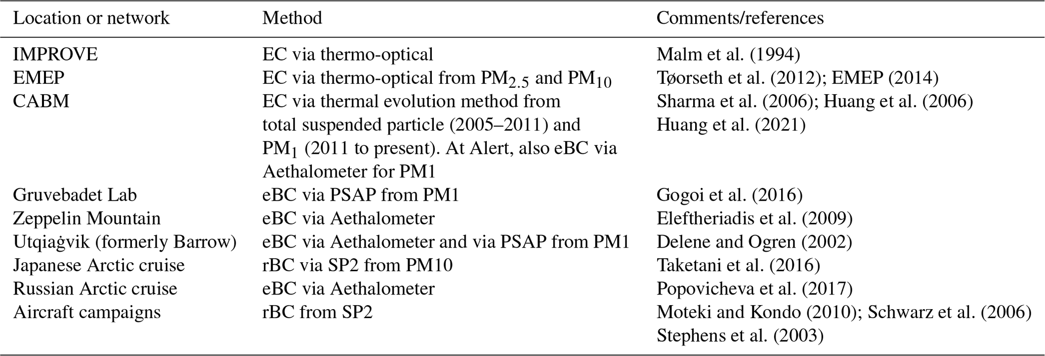
For SLCFs other than Arctic BC, Table B2 summarizes some information about the observation networks.
Table B2Information about SLCF measurements from monitoring networks used for model evaluation in the Northern Hemisphere.
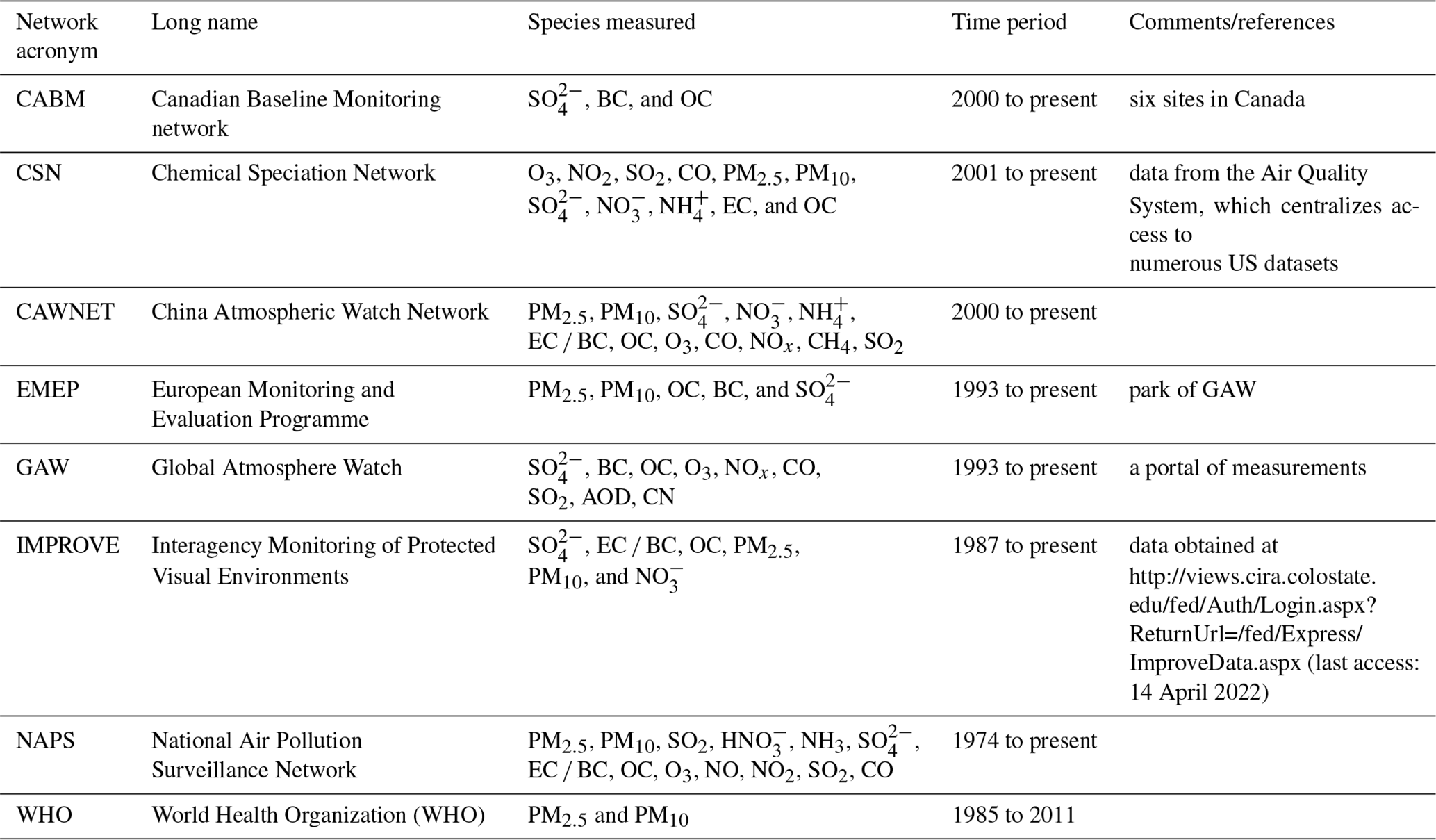
The models' output files in NetCDF format from the simulations used in this project can be found here: http://crd-data-donnees-rdc.ec.gc.ca/CCCMA/products/AMAP/ (Canadian Centre for Climate Modelling and analysis, 2022a).
Some of the models' code are available online at the following locations. CanAM5-PAM: https://gitlab.com/cccma (Canadian Centre for Climate Modelling and analysis, 2022b). CESM2: https://www.cesm.ucar.edu/models/cesm2/ (UCAR, 2022a). ECHAM-SALSA: The codes used for the ECHAM-SALSA simulations are available from the ECHAM-HAMMOZ repository under https://redmine.hammoz.ethz.ch/projects/hammoz/repository/1/show/echam6-hammoz/branches/fmi/AMAP/AMAP_evaluation (Center for Climate Systems Modeling – C2SM at ETH Zurich, 2022), after obtaining the HAMMOZ license. FLEXPART: https://www.flexpart.eu (GNU General Public License, 2022). GEOS-Chem: http://wiki.seas.harvard.edu/geos-chem/index.php/GEOS-Chem_12#12.3.2 (Harvard University, 2022). GISS-E2.1: https://www.giss.nasa.gov/tools/modelE/ (NASA, 2022a). NorESM: https://github.com/NorESMhub/NorESM (NorESM Climate Modeling Consortium, 2022). Oslo CTM: https://github.com/NordicESMhub/OsloCTM3 (Section for Meteorology and Oceanography, 2022). The other models' code may be available upon request.
The model evaluation programs can be found on GitLab here: https://gitlab.com/cynwhaley/amap-slcf-model-evaluation (Whaley et al., 2022b).
The surface monitoring datasets are available online. WDCGG for CH4: https://gaw.kishou.go.jp/login/user (Global Atmosphere Watch, 2022). EBAS for European (EMEP) and several Arctic locations: http://ebas.nilu.no/ (Norwegian Institute for Air Research, 2022). NAPS: https://open.canada.ca/data/en/dataset/1b36a356-defd-4813-acea-47bc3abd859b (Environment and Climate Change Canada, 2022). IMPROVE: https://views.cira.colostate.edu/fed/Express/ImproveData.aspx (Federal Land Manager Environmental Database, 2022). Beijing Air Quality for China: https://quotsoft.net/air/ (Xiaolei and Weibo, 2022). PM2.5 from the US embassy in China from the data portal: http://www.stateair.net (U.S. Department of State Air Quality Monitoring Program, 2022).
The satellite measurement data used in this study are available online. ACE-FTS v4.1 measurements are available, following registration, from http://www.ace.uwaterloo.ca (University of Waterloo, 2022). TES: https://tes.jpl.nasa.gov/tes/data/products/lite (NASA, 2022b). MOPITT: https://www2.acom.ucar.edu/mopitt/products (UCAR, 2022b).
The supplement related to this article is available online at: https://doi.org/10.5194/acp-22-5775-2022-supplement.
CHW organized the model–measurement comparisons in the AMAP SLCF expert group, led the trace gas model evaluations, and wrote the paper with contributions from co-authors. RM developed and ran the aerosol model–measurement comparison scripts, including the ship-based BC measurements, and did the aerosol analysis. KvS led the AMAP SLCF modeling strategy and developed and ran the CanAM5-PAM model. SE and NE provided FLEXPART model output, and SE did the model–measurement comparisons for BC and SO deposition. DWP developed the CIS tool for BC aircraft model–measurement comparisons, and BW used the tool and did the model–aircraft comparisons and analysis. LNS did the ACE-FTS trace gas model comparisons, and KAW provided guidance on ACE-FTS data quality, usage, and model–measurement comparisons. MF co-led the AMAP model strategy and ran CESM. LP provided additional CESM runs. DAP developed and ran CMAM. YP and MW provided CIESM-MAM7 model output; JC provided DEHM model output; TK provided ECHAM-SALSA model output; ST and MG provided EMEP-MSC-W model output and some analysis. UI, GF, and KT provided the GISS-E2.1 model output; WG and SB provided the GEM-MACH model output; JSF, RYC, and XD provided the GEOS-Chem model output; JL provided the MATCH model output; MAT provided the MATCH-SALSA model output; NO provided the MRI-ESM2 model output; MS and SK provided the NorESM model output; RS provided the OsloCTM model output; SA and ST provided UKESM1 model output; and KSL, JCR, TO, and LM provided WRF-Chem model output. SS and LH provided Alert datasets; VV and SB provided Gruvebadet datasets; OP provided Russian cruise ship measurements; FT and YK provided the Japanese ship measurements; HS and AM provided Villum Research Station datasets; JS provided aerosol datasets and expertise. TWG and SMD wrote and developed the trace gas model–measurement comparison scripts.
At least one of the (co-)authors is a member of the editorial board of Atmospheric Chemistry and Physics. The peer-review process was guided by an independent editor, and the authors also have no other competing interests to declare.
PM2.5 observation from the US embassy in China belongs to the US Department of State, is not fully verified or validated, and could be subject to changes, corrections, or errors.
Publisher's note: Copernicus Publications remains neutral with regard to jurisdictional claims in published maps and institutional affiliations.
This article is part of the special issue “Arctic climate, air quality, and health impacts from short-lived climate forcers (SLCFs): contributions from the AMAP Expert Group (ACP/BG inter-journal SI)”. It is not associated with a conference.
The work reflected in this publication was produced with the financial support of the Arctic Monitoring and Assessment Programme (AMAP). The authors would like to thank all operators and technicians at the Arctic stations for the collection of observational data. Thanks are also due to the following people for providing us with data: Mauro Mazzola, Stefania Gilardoni, and Angelo Lupi from the Institute of Polar Sciences for eBC measurements at Gruvebadet lab; and Mirko Severi from the University of Florence for SO measurements at Gruvebadet. Fairbanks aerosol measurements came from William Simpson. For Villum data, we acknowledge the Aarhus University Department of Environmental Science (ENVS). NOAA/ESRL/GMD, EMEP (http://ebas.nilu.no, last access: 14 April 2022), and the WMO GAW network are acknowledged for Barrow and Zeppelin observational datasets. The ACE-FTS is a Canadian-led mission mainly supported by the Canadian Space Agency (CSA). IMPROVE is a collaborative association of state, tribal, and federal agencies, as well as international partners. The US Environmental Protection Agency is the primary funding source, with contracting and research support from the National Park Service. The Air Quality Group at the University of California, Davis, is the central analytical laboratory, with ion analysis provided by the Research Triangle Institute and carbon analysis provided by the Desert Research Institute. Julia Schmale holds the Ingvar Kamprad Chair for Extreme Environments Research sponsored by Ferring Pharmaceuticals. The ECHAM-HAMMOZ model is developed by a consortium composed of ETH Zurich, the Max-Planck-Institut für Meteorologie, Forschungszentrum Jülich, the University of Oxford, the Finnish Meteorological Institute, and the Leibniz Institute for Tropospheric Research; it is managed by the Center for Climate Systems Modeling (C2SM) at ETH Zurich.
Assessments
from the Russian ship-based campaign were performed with
the support of RFBR project no. 20-55-12001 and according to the
development program of the Interdisciplinary Scientific and Educational
School of M.V. Lomonosov Moscow State University “Future
Planet and Global Environmental Change”.
Development of the methodology for aethalometric data treatment was supported by RSF project no. 19-77-30004. The
BC observations on R/V Mirai were supported by the Ministry
of Education, Culture, Sports, Science and Technology (MEXT),
Japan (Arctic Challenge for Sustainability (ArCS) project). Contributions
by SMHI were funded by the Swedish Environmental
Protection Agency under contract NV-03174-20 and the Swedish
Climate and Clean Air Research program (SCAC) as well as partly
by the Swedish National Space Board (NORD-SLCP, grant agreement
ID: 94/16) and the EU Horizon 2020 project Integrated Arctic
Observing System (INTAROS, grant agreement ID: 727890). Work on ACE-FTS analysis
was supported by the Natural Sciences and Engineering Research
Council of Canada (NSERC). Julia Schmale
received funding from the Swiss National Science Foundation
(project no. 200021_188478). Duncan Watson-Parris received
funding from NERC projects NE/P013406/1 (A-CURE) and
NE/S005390/1 (ACRUISE) as well as funding from the European
Union's Horizon 2020 research and innovation program iMIRACLI
under Marie Skłodowska-Curie grant agreement no. 860100. LATMOS has been supported by the EU iCUPE (Integrating
and Comprehensive Understanding on Polar Environments) project
(grant agreement no. 689443) under the European Network for Observing
our Changing Planet (ERA-Planet), as well as access to
IDRIS HPC resources (GENCI allocation A009017141) and the
IPSL mesoscale computing center (CICLAD: Calcul Intensif pour
le CLimat, l’Atmosphère et la Dynamique) for model simulations.
Naga Oshima was supported by the Japan Society for the Promotion of Science
KAKENHI (grant nos. JP18H03363, JP18H05292, and
JP21H03582), the Environment Research and Technology Development
Fund (grant nos. JPMEERF20202003 and JPMEERF20205001) of
the Environmental Restoration and Conservation Agency of Japan,
the Arctic Challenge for Sustainability II (ArCS II) under program
grant no. JPMXD1420318865, and a grant for the Global Environmental
Research Coordination System from the Ministry of the
Environment, Japan (MLIT1753). The research with GISS-E2.1 has
been supported by the Aarhus University Interdisciplinary Centre
for Climate Change (iClimate) OH fund (no. 2020-0162731), the
FREYA project funded by the Nordic Council of Ministers (grant
agreement nos. MST-227-00036 and MFVM-2019-13476), and the
EVAM-SLCF funded by the Danish Environmental Agency (grant
agreement no. MST-112-00298). Jesper Christensen (for DEHM
model) received funding from the Danish Environmental Protection Agency
(DANCEA funds for Environmental Support to the Arctic Region
project; grant no. 2019-7975). Maria Sand has been supported by the Research Council of Norway
(grant 315195, ACCEPT).
Publisher's note: the article processing charges for this publication were not paid by a Russian or Belarusian institution.
This paper was edited by Frank Dentener and reviewed by two anonymous referees.
Abdul-Razzak, H. and Ghan, S. J.: A parameterization of aerosol activation 3. Sectional representation, J. Geophys. Res., 107, AAC1.1–AAC1.6, https://doi.org/10.1029/2001JD000483, 2002. a
Alexander, B., Park, R. J., Jacob, D. J., and Gong, S.: Transition metal-catalyzed oxidation of atmospheric sulfur: Global implications for the sulfur budget, J. Geophys. Res.-Atmos., 114, D02309, https://doi.org/10.1029/2008JD010486, 2009. a
Allen, R. J. and Landuyt, W.: The vertical distribution of black carbon in CMIP5 models: Comparison to observations and the importance of convective transport, J. Geophys. Res.-Atmos., 119, 4808–4835, https://doi.org/10.1002/2014JD021595, 2014. a
Amann, M., Bertok, I., Borken-Kleefled, J., Cofala, J., Heyes, C., Höglund-Isaksson, L., Klimont, Z., Nguyen, B., Posch, M., Rafaj, P., Sandler, R., Schöpp, W., Wagner, F., and Winiwarter, W.: Cost-effective control of air quality and greenhouse gases inEurope: Modelling and policy applications, Environ. Modell. Softw., 26, 1489–1501, 2011. a
AMAP: Arctic Monitoring and Assessment Programme, Assessment 2015: Black carbon and ozone as Arctic climate forcers, Technical report, AMAP, Oslo, Norway, vii + 116 pp., https://www.amap.no/documents/doc/amap-assessment-2015-black-carbon-and-ozone-as-arctic-climate-forcers/1299 (last access: 14 April 2022), 2015a. a, b, c, d, e
AMAP: Arctic Monitoring and Assessment Programme, Assessment 2015: Methane as an Arctic climate forcer, Technical report, AMAP, Norway, vii + 139 pp., https://www.amap.no/documents/doc/amap-assessment-2015-methane-as-an-arctic-climate-forcer/1285 (last access: 14 April 2022), 2015b. a
AMAP: Arctic Climate Change Update 2021: Key Trends and Impacts. Summary for Policy-makers, Tech. rep., Arctic Monitoring and Assessment Programme (AMAP), Tromsøo, Norway, https://www.amap.no/documents/doc/arctic-climate-change-update-2021-key-trends-and-impacts.-summary-for-policy-makers/3508 (last access: 14 April 2022), 2021. a
AMAP: Arctic Monitoring and Assessment Programme, Assessment 2022: short-lived climate forcers, Technical report, AMAP, Oslo, Norway, https://www.amap.no/ (last access: 14 April 2022), in press, 2022. a, b, c, d, e, f, g, h, i, j, k
Amos, H. M., Jacob, D. J., Holmes, C. D., Fisher, J. A., Wang, Q., Yantosca, R. M., Corbitt, E. S., Galarneau, E., Rutter, A. P., Gustin, M. S., Steffen, A., Schauer, J. J., Graydon, J. A., Louis, V. L. St., Talbot, R. W., Edgerton, E. S., Zhang, Y., and Sunderland, E. M.: Gas-particle partitioning of atmospheric Hg(II) and its effect on global mercury deposition, Atmos. Chem. Phys., 12, 591–603, https://doi.org/10.5194/acp-12-591-2012, 2012. a
Andersson, C., Langner, J., and Bergström, R.: Interannual variation and trends in air pollution over Europe due to climate variability during 1958-2001 simulated with a regional CTM coupled to the ERA-40 reanalysis, Tellus B, 59, 77–98, 2007. a, b, c
Andersson, C., Bergström, R., Bennet, C., Robertson, L., Thomas, M., Korhonen, H., Lehtinen, K. E. J., and Kokkola, H.: MATCH-SALSA – Multi-scale Atmospheric Transport and CHemistry model coupled to the SALSA aerosol microphysics model – Part 1: Model description and evaluation, Geosci. Model Dev., 8, 171–189, https://doi.org/10.5194/gmd-8-171-2015, 2015. a
Andres, R. J. and Kasgnoc, A. D.: A time-averaged inventory of subaerial volcanic sulfur emissions, J. Geophys. Res.-Atmos., 103, 25251–25261, https://doi.org/10.1029/98JD02091, 1998. a
Archibald, A. T., O'Connor, F. M., Abraham, N. L., Archer-Nicholls, S., Chipperfield, M. P., Dalvi, M., Folberth, G. A., Dennison, F., Dhomse, S. S., Griffiths, P. T., Hardacre, C., Hewitt, A. J., Hill, R. S., Johnson, C. E., Keeble, J., Köhler, M. O., Morgenstern, O., Mulcahy, J. P., Ordóñez, C., Pope, R. J., Rumbold, S. T., Russo, M. R., Savage, N. H., Sellar, A., Stringer, M., Turnock, S. T., Wild, O., and Zeng, G.: Description and evaluation of the UKCA stratosphere–troposphere chemistry scheme (StratTrop vn 1.0) implemented in UKESM1, Geosci. Model Dev., 13, 1223–1266, https://doi.org/10.5194/gmd-13-1223-2020, 2020. a
Arnold, S., Law, K., Brock, C., Thomas, J., Starkweather, S., von Salzen, K., Stohl, A., Sharma, S., Lund, M., Flanner, M., Petäjä, T., Tanimoto, H., Gamble, J., Dibb, J., Melamed, M., Johnson, N., Fidel, M., Tynkkynen, V.-P., Baklanov, A., Eckhardt, S., Monks, S., Browse, J., and Bozem, H.: Arctic air pollution: Challenges and opportunities for the next decade, Elementa, 4, 000104, https://doi.org/10.12952/journal.elementa.000104, 000104, 2016. a
Arnold, S. R., Emmons, L. K., Monks, S. A., Law, K. S., Ridley, D. A., Turquety, S., Tilmes, S., Thomas, J. L., Bouarar, I., Flemming, J., Huijnen, V., Mao, J., Duncan, B. N., Steenrod, S., Yoshida, Y., Langner, J., and Long, Y.: Biomass burning influence on high-latitude tropospheric ozone and reactive nitrogen in summer 2008: a multi-model analysis based on POLMIP simulations, Atmos. Chem. Phys., 15, 6047–6068, https://doi.org/10.5194/acp-15-6047-2015, 2015. a, b
Barrie, L. A., Bottenheim, J. W., Schnell, R. C., Crutzen, P. J., and Rasmussen, R. A.: Ozone destruction and photochemical-reactions at polar sunrise in the lower Arctic atmosphere, Nature, 334, 138–141, 1988. a
Bauer, S. E. and Koch, D.: Impact of heterogeneous sulfate formation at mineral dust surfaces on aerosol loads and radiative forcing in the Goddard Institute for Space Studies general circulation model, J. Geophys. Res.-Atmos., 110, D17202, https://doi.org/10.1029/2005JD005870, 2005. a, b
Bauer, S. E., Koch, D., Unger, N., Metzger, S. M., Shindell, D. T., and Streets, D. G.: Nitrate aerosols today and in 2030: a global simulation including aerosols and tropospheric ozone, Atmos. Chem. Phys., 7, 5043–5059, https://doi.org/10.5194/acp-7-5043-2007, 2007a. a
Bauer, S. E., Mishchenko, M. I., Lacis, A. A., Zhang, S., Perlwitz, J., and Metzger, S. M.: Do sulfate and nitrate coatings on mineral dust have important effects on radiative properties and climate modeling?, J. Geophys. Res.-Atmos., 112, D06307, https://doi.org/10.1029/2005JD006977, 2007b. a
Bauer, S. E., Bausch, A., Nazarenko, L., Tsigaridis, K., Xu, B., Edwards, R., Bisiaux, M., and McConnell, J.: Historical and future black carbon deposition on the three ice caps: Ice core measurements and model simulations from 1850 to 2100, J. Geophys. Res.-Atmos., 118, 7948–7961, https://doi.org/10.1002/jgrd.50612, 2013. a, b
Bauer, S. E., Tsigaridis, K., Faluvegi, G., Kelley, M., Lo, K. K., Miller, R. L., Nazarenko, L., Schmidt, G. A., and Wu, J.: Historical (1850–2014) Aerosol Evolution and Role on Climate Forcing Using the GISS ModelE2.1 Contribution to CMIP6, J. Adv. Model. Earth Sy., 12, e2019MS001978, https://doi.org/10.1029/2019MS001978, 2020. a, b
Bauguitte, S.: Facility for airborne atmospheric measurements: Science instruments, https://www.faam.ac.uk/ (last access: 14 April 2022), 2014. a, b
Beer, R.: TES on the aura mission: scientific objectives, measurements, and analysis overview, IEEE T. Geosci. Remote, 44, 1102–1105, https://doi.org/10.1109/TGRS.2005.863716, 2006. a
Bentsen, M., Bethke, I., Debernard, J. B., Iversen, T., Kirkevåg, A., Seland, Ø., Drange, H., Roelandt, C., Seierstad, I. A., Hoose, C., and Kristjánsson, J. E.: The Norwegian Earth System Model, NorESM1-M – Part 1: Description and basic evaluation of the physical climate, Geosci. Model Dev., 6, 687–720, https://doi.org/10.5194/gmd-6-687-2013, 2013. a, b
Bergström, R., Denier van der Gon, H. A. C., Prévôt, A. S. H., Yttri, K. E., and Simpson, D.: Modelling of organic aerosols over Europe (2002–2007) using a volatility basis set (VBS) framework: application of different assumptions regarding the formation of secondary organic aerosol, Atmos. Chem. Phys., 12, 8499–8527, https://doi.org/10.5194/acp-12-8499-2012, 2012. a, b
Bernath, P. F., McElroy, C. T., Abrams, M. C., Boone, C. D., Butler, M., Camy-Peyret, C., Carleer, M., Clerbaux, C., Coheur, P.-F., Colin, R., DeCola, P., DeMazière, M., Drummond, J. R., Dufour, D., Evans, W. F. J., Fast, H., Fussen, D., Gilbert, K., Jennings, D. E., Llewellyn, E. J., Lowe, R. P., Mahieu, E., McConnell, J. C., McHugh, M., McLeod, S. D., Michaud, R., Midwinter, C., Nassar, R., Nichitiu, F., Nowlan, C., Rinsland, C. P., Rochon, Y. J., Rowlands, N., Semeniuk, K., Simon, P., Skelton, R., Sloan, J. J., Soucy, M.-A., Strong, K., Tremblay, P., Turnbull, D., Walker, K. A., Walkty, I., Wardle, D. A., Wehrle, V., Zander, R., and Zou, J.: Atmospheric Chemistry Experiment (ACE): Mission overview, Geophys. Res. Lett., 32, L15S01, https://doi.org/10.1029/2005GL022386, 2005. a
Berrisford, P., Dee, D., Poli, P., Brugge, R., Fielding, K., Fuentes, M., Kållberg, P., Kobayashi, S., Uppala, S., and Simmons, A.: The ERA-Interim archive Version 2.0, technical report, U.S. EPA, OAQPS, Shinfield Park, Reading, https://www.ecmwf.int/en/elibrary/8174-era-interim-archive-version-20 (last access: 14 April 2022), 2011. a
Bey, I., Jacob, D. J., Yantosca, R. M., Logan, J. A., Field, B. D., Fiore, A. M., Li, Q., Liu, H. Y., Mickley, L. J., and Schultz, M. G.: Global modeling of tropospheric chemistry with assimilated meteorology: Model description and evaluation, J. Geophys. Res., 106, 23073–23095, https://doi.org/10.1029/2001JD000807, 2001. a, b
Biraud, S. C.: Carbon Monoxide Mixing Ratio System Handbook, Tech. rep., U.S. Dept. of Energy, ARM Clim. Res. Facil., Washington, D.C., https://digital.library.unt.edu/ark:/67531/metadc846059/ (last access: 14 April 2022), 2011. a
Bottenheim, J. W., Gallant, A. G., and Brice, K. A.: Measurements of NOy species and O3 at 82∘ N latitude, Geophys. Res. Lett., 13, 113–116, 1986. a
Brandt, J., Silver, J., Frohn, L. M., Geels, C., Gross, A., Hansen, A. B., Hansen, K. M., Hedegaard, G. B., Skjøoth, C. A., Villadsen, H., Zare, A., and Christensen, J. H.: An integrated model study for Europe and North America using the Danish Eulerian Hemispheric Model with focus on intercontinental transport of air pollution, Atmos. Environ., 53, 156–176, 2012. a, b
Breider, T. J., Mickley, L. J., Jacob, D. J., Wang, Q., Fisher, J. A., Chang, R. Y.-W., and Alexander, B.: Annual distributions and sources of Arctic aerosol components, aerosol optical depth, and aerosol absorption, J. Geophys. Res.-Atmos., 119, 4107–4124, https://doi.org/10.1002/2013JD020996, 2014. a
Breider, T. J., Mickley, L. J., Jacob, D. J., Ge, C., Wang, J., Payer Sulprizio, M., Croft, B., Ridley, D. A., McConnell, J. R., Sharma, S., Husain, L., Dutkiewicz, V. A., Eleftheriadis, K., Skov, H., and Hopke, P. K.: Multidecadal trends in aerosol radiative forcing over the Arctic: Contribution of changes in anthropogenic aerosol to Arctic warming since 1980, J. Geophys. Res.-Atmos., 122, 3573–3594, https://doi.org/10.1002/2016JD025321, 2017. a
Brock, C. A., Cozic, J., Bahreini, R., Froyd, K. D., Middlebrook, A. M., McComiskey, A., Brioude, J., Cooper, O. R., Stohl, A., Aikin, K. C., de Gouw, J. A., Fahey, D. W., Ferrare, R. A., Gao, R.-S., Gore, W., Holloway, J. S., Hübler, G., Jefferson, A., Lack, D. A., Lance, S., Moore, R. H., Murphy, D. M., Nenes, A., Novelli, P. C., Nowak, J. B., Ogren, J. A., Peischl, J., Pierce, R. B., Pilewskie, P., Quinn, P. K., Ryerson, T. B., Schmidt, K. S., Schwarz, J. P., Sodemann, H., Spackman, J. R., Stark, H., Thomson, D. S., Thornberry, T., Veres, P., Watts, L. A., Warneke, C., and Wollny, A. G.: Characteristics, sources, and transport of aerosols measured in spring 2008 during the aerosol, radiation, and cloud processes affecting Arctic Climate (ARCPAC) Project, Atmos. Chem. Phys., 11, 2423–2453, https://doi.org/10.5194/acp-11-2423-2011, 2011. a
Brown, S. S., Ryerson, T. B., Wollny, A. G., Brock, C. A., Peltier, R., Sullivan, A. P., Weber, R. J., Dubé, W. P., Trainer, M., Meagher, J. F., Fehsenfeld, F. C., and Ravishankara, A. R.: Variability in Nocturnal Nitrogen Oxide Processing and Its Role in Regional Air Quality, Science, 311, 67–70, https://doi.org/10.1126/science.1120120, 2006. a
Browse, J., Carslaw, K. S., Arnold, S. R., Pringle, K., and Boucher, O.: The scavenging processes controlling the seasonal cycle in Arctic sulphate and black carbon aerosol, Atmos. Chem. Phys., 12, 6775–6798, https://doi.org/10.5194/acp-12-6775-2012, 2012. a
Bush, E. and Lemmen, D. S.: Canada's Changing Climate Report, Tech. rep., Government of Canada, Ottawa, ON, Canada, https://geoscan.nrcan.gc.ca/starweb/geoscan/servlet.starweb?path=geoscan/fulle.web&search1=R=314614 (last access: 14 April 2022), 2019. a
Canadian Centre for Climate Modelling and analysis (CCCma): AMAP SLCF models output in NetCDF format, CCCma [data set], http://crd-data-donnees-rdc.ec.gc.ca/CCCMA/products/AMAP/, last access: 14 April 2022a. a
Canadian Centre for Climate Modelling and analysis (CCCma): CanAM5-PAM model code, CCCma [code], https://gitlab.com/cccma, last access: 14 April 2022b. a
Cassiani, M., Stohl, A., and Brioude, J.: Lagrangian Stochastic Modelling of Dispersion in the Convective Boundary Layer with Skewed Turbulence Conditions and a Vertical Density Gradient: Formulation and Implementation in the FLEXPART Model, Bound.-Lay. Meteorol., 154, 367–390, https://doi.org/10.1007/s10546-014-9976-5, 2014. a
Cavalli, F., Viana, M., Yttri, K. E., Genberg, J., and Putaud, J.-P.: Toward a standardised thermal-optical protocol for measuring atmospheric organic and elemental carbon: the EUSAAR protocol, Atmos. Meas. Tech., 3, 79–89, https://doi.org/10.5194/amt-3-79-2010, 2010. a
Center for Climate Systems Modeling – C2SM at ETH, Zurich: ECHAM-SALSA model code, C2SM [code], https://redmine.hammoz.ethz.ch/projects/hammoz/repository/1/show/echam6-hammoz/branches/fmi/AMAP/AMAP_evaluation, last access: 14 April 2022. a
Chan, T. W., Huang, L., Banwait, K., Zhang, W., Ernst, D., Wang, X., Watson, J. G., Chow, J. C., Green, M., Czimczik, C. I., Santos, G. M., Sharma, S., and Jones, K.: Inter-comparison of elemental and organic carbon mass measurements from three North American national long-term monitoring networks at a co-located site, Atmos. Meas. Tech., 12, 4543–4560, https://doi.org/10.5194/amt-12-4543-2019, 2019. a, b
Charron, M., Polavarapu, S., Buehner, M., Vaillancourt, P. A., Charette, C., Roch, M., Morneau, J., Garand, L., Aparicio, J. M., MacPherson, S., Pellerin, S., St-James, J., and Heilliette, S.: The Stratospheric Extension of the Canadian Global Deterministic Medium-Range Weather Forecasting System and Its Impact on Tropospheric Forecasts, Mon. Weather Rev., 140, 1924–1944, https://doi.org/10.1175/MWR-D-11-00097.1, 2012. a
Chen, J., Anderson, K., Pavlovic, R., Moran, M. D., Englefield, P., Thompson, D. K., Munoz-Alpizar, R., and Landry, H.: The FireWork v2.0 air quality forecast system with biomass burning emissions from the Canadian Forest Fire Emissions Prediction System v2.03, Geosci. Model Dev., 12, 3283–3310, https://doi.org/10.5194/gmd-12-3283-2019, 2019. a
Chen, Q., Schmidt, J. A., Shah, V., Jaegle, L., Sherwen, T., and Alexander, B.: Sulfate production by reactive bromine: Implications for the global sulfur and reactive bromine budgets, Geophys. Res. Lett., 44, 7069–7078, https://doi.org/10.1002/2017GL073812, 2017. a
Chow, J. C., Watson, J. G., Pritchett, L. C., Pierson, W. R., Frazier, C. a., and Purcell, R. G.: The dri thermal/optical reflectance carbon analysis system: description, evaluation and applications in U.S. Air quality studies, Atmos. Environ., 27, 1185–1201, https://doi.org/10.1016/0960-1686(93)90245-T, 1993. a
Chow, J. C., Watson, J. G., Crow, D., Lowenthal, D. H., and Merrifield, T.: Comparison of IMPROVE and NIOSH Carbon Measurements, Aerosol Sci. Tech., 34, 23–34, https://doi.org/10.1080/02786820119073, 2001. a
Chow, J. C., Watson, J. G., Chen, L.-W. A., Arnott, W. P., Moosmüller, H., and Fung, K. K.: Equivalence of elemental carbon by Thermal/Optical Reflectance and Transmittance with different temperature protocols, Environ. Sci. Technol., 38, 4414–4422, https://doi.org/10.1021/es034936u, 2004. a
Christensen, J. H.: The Danish Eulerian hemispheric model – A three-dimensional air pollution model used for the Arctic, Atmos. Environ., 31, 4169–4191, 1997. a, b
Côté, J., Desmarais, J.-G., Gravel, S., Méthot, A., Patoine, A., Roch, M., and Staniforth, A.: The Operational CMC-MRB Global Environmental Multiscale (GEM) Model. Part II: Results, Mon. Weather Rev., 126, 1397–1418, https://doi.org/10.1175/1520-0493(1998)126<1397:TOCMGE>2.0.CO;2, 1998a. a
Côté, J., Gravel, S., Méthot, A., Patoine, A., Roch, M., and Staniforth, A.: The Operational CMC-MRB Global Environmental Multiscale (GEM) Model. Part I: Design Considerations and Formulation, Mon. Weather Rev., 126, 1373–1395, https://doi.org/10.1175/1520-0493(1998)126<1373:TOCMGE>2.0.CO;2, 1998b. a
Dabek-Zlotorzynska, E., Dann, T. F., Kalyani Martinelango, P., Celo, V., Brook, J. R., Mathieu, D., Ding, L., and Austin, C. C.: Canadian National Air Pollution Surveillance (NAPS) PM2.5 speciation program: Methodology and PM2.5 chemical composition for the years 2003–2008, Atmos. Environ., 45, 673–686, https://doi.org/10.1016/j.atmosenv.2010.10.024, 2011. a
Damian, V., Sandu, A., Damian, M., Potra, F., and Carmichael, G.: The Kinetic PreProcessor KPP-A software environment for solving chemical kinetics, Comput. Chem. Eng., 26, 1567–1579, 2002. a
Danabasoglu, G., Lamarque, J., Bacmeister, J., Bailey, D. A., DuVivier, A. K., and Edwards, J.: The Community Earth System Model Version 2 (CESM2), J. Adv. Model. Earth Sy., 12, e2019MS001916, https://doi.org/10.1029/2019MS001916, 2020. a, b
Davis, J. M., Bhave, P. V., and Foley, K. M.: Parameterization of N2O5 reaction probabilities on the surface of particles containing ammonium, sulfate, and nitrate, Atmos. Chem. Phys., 8, 5295–5311, https://doi.org/10.5194/acp-8-5295-2008, 2008. a
Dee, D. P., Uppala, S. M., Simmons, A. J., Berrisford, P., Polia, P., Kobayashib, S., Andraec, U., Balmaseda, M. A., Balsamo, G., P., B., Bechtold, P., Beljaars, A. C. M., van de Bergd, L., Bidlot, J., Bormann, N., Delsol, C., Dragani, R., Fuentes, M., Geer, A. J., Haimberger, L., Healy, S. B., Hersbach, H., Hó́lm, E. V., Isaksen, L., Kållberg, P., Köhler, M., Matricardi, M., McNally, A. P., Monge-Sanz, B. M., Morcrette, J.-J., Park, B.-K., Peubey, C., de Rosnay, P., Tavolato, C., Thépaut, J.-N., and Vitart, F.: The ERA-Interim reanalysis: configuration and performance of the data assimilation system, Q. J. Roy. Meteor. Soc., 137, 553–597, https://doi.org/10.1002/qj.828, 2011. a
Deeter, M. N., Edwards, D. P., Francis, G. L., Gille, J. C., Mao, D., Martínez-Alonso, S., Worden, H. M., Ziskin, D., and Andreae, M. O.: Radiance-based retrieval bias mitigation for the MOPITT instrument: the version 8 product, Atmos. Meas. Tech., 12, 4561–4580, https://doi.org/10.5194/amt-12-4561-2019, 2019. a
Delene, D. J. and Ogren, J. A.: Variability of Aerosol Optical Properties at Four North American Surface Monitoring Sites, J. Atmos. Sci., 59, 1135–1150, https://doi.org/10.1175/1520-0469(2002)059<1135:VOAOPA>2.0.CO;2, 2002. a
Dentener, F., Kinne, S., Bond, T., Boucher, O., Cofala, J., Generoso, S., Ginoux, P., Gong, S., Hoelzemann, J. J., Ito, A., Marelli, L., Penner, J. E., Putaud, J.-P., Textor, C., Schulz, M., van der Werf, G. R., and Wilson, J.: Emissions of primary aerosol and precursor gases in the years 2000 and 1750 prescribed data-sets for AeroCom, Atmos. Chem. Phys., 6, 4321–4344, https://doi.org/10.5194/acp-6-4321-2006, 2006. a, b
Dlugokencky, E. J., Steele, L. P., Lang, P. M., and Masarie, K. A.: The growth rate and distribution of atmospheric methane, J. Geophys. Res.-Atmos., 99, 17021–17043, https://doi.org/10.1029/94JD01245, 1994. a
Duncan Fairlie, T., Jacob, D. J., and Park, R. J.: The impact of transpacific transport of mineral dust in the United States, Atmos. Environ., 41, 1251–1266, https://doi.org/10.1016/j.atmosenv.2006.09.048, 2007. a
Eckhardt, S., Quennehen, B., Olivié, D. J. L., Berntsen, T. K., Cherian, R., Christensen, J. H., Collins, W., Crepinsek, S., Daskalakis, N., Flanner, M., Herber, A., Heyes, C., Hodnebrog, Ø., Huang, L., Kanakidou, M., Klimont, Z., Langner, J., Law, K. S., Lund, M. T., Mahmood, R., Massling, A., Myriokefalitakis, S., Nielsen, I. E., Nøjgaard, J. K., Quaas, J., Quinn, P. K., Raut, J.-C., Rumbold, S. T., Schulz, M., Sharma, S., Skeie, R. B., Skov, H., Uttal, T., von Salzen, K., and Stohl, A.: Current model capabilities for simulating black carbon and sulfate concentrations in the Arctic atmosphere: a multi-model evaluation using a comprehensive measurement data set, Atmos. Chem. Phys., 15, 9413–9433, https://doi.org/10.5194/acp-15-9413-2015, 2015. a, b, c
Eleftheriadis, K., Vratolis, S., and Nyeki, S.: Aerosol black carbon in the European Arctic: Measurements at Zeppelin station, Ny-Ålesund, Svalbard from 1998–2007, Geophys. Res. Lett., 36, L02809, https://doi.org/10.1029/2008GL035741, 2009. a
EMEP: EMEP manual for sampling and chemical analysis, Manual, Norwegian Institute for Air Research, Oslo, Norway, https://projects.nilu.no/ccc/manual/ (last access: 14 April 2022), 2014. a
Emmons, L. K., Walters, S., Hess, P. G., Lamarque, J.-F., Pfister, G. G., Fillmore, D., Granier, C., Guenther, A., Kinnison, D., Laepple, T., Orlando, J., Tie, X., Tyndall, G., Wiedinmyer, C., Baughcum, S. L., and Kloster, S.: Description and evaluation of the Model for Ozone and Related chemical Tracers, version 4 (MOZART-4), Geosci. Model Dev., 3, 43–67, https://doi.org/10.5194/gmd-3-43-2010, 2010. a, b
Emmons, L. K., Arnold, S. R., Monks, S. A., Huijnen, V., Tilmes, S., Law, K. S., Thomas, J. L., Raut, J.-C., Bouarar, I., Turquety, S., Long, Y., Duncan, B., Steenrod, S., Strode, S., Flemming, J., Mao, J., Langner, J., Thompson, A. M., Tarasick, D., Apel, E. C., Blake, D. R., Cohen, R. C., Dibb, J., Diskin, G. S., Fried, A., Hall, S. R., Huey, L. G., Weinheimer, A. J., Wisthaler, A., Mikoviny, T., Nowak, J., Peischl, J., Roberts, J. M., Ryerson, T., Warneke, C., and Helmig, D.: The POLARCAT Model Intercomparison Project (POLMIP): overview and evaluation with observations, Atmos. Chem. Phys., 15, 6721–6744, https://doi.org/10.5194/acp-15-6721-2015, 2015. a, b
Emmons, L. K., Schwantes, R. H., Orlando, J. J., Tyndall, G., Kinnison, D., Lamarque, J.-F., Marsh, D., Mills, M. J., Tilmes, S., Bardeen, C., Buchholz, R. R., Conley, A., Gettelman, A., Garcia, R., Simpson, I., Blake, D. R., Meinardi, S., and Pétron, G.: The Chemistry Mechanism in the Community Earth System Model Version 2 (CESM2), J. Adv. Model. Earth Sy., 12, e2019MS001882, https://doi.org/10.1029/2019MS001882, 2020a. a
Emmons, L. K., Schwantes, R. H., Orlando, J. J., Tyndall, G., Kinnison, D., Lamarque, J.-F., Marsh, D., Mills, M. J., Tilmes, S., Bardeen, C., Buchholz, R. R., Conley, A., Gettelman, A., Garcia, R., Simpson, I., Blake, D. R., Meinardi, S., and Pétron, G.: The Chemistry Mechanism in the Community Earth System Model Version 2 (CESM2), J. Adv. Model. Earth Sy., 12, e2019MS001882, https://doi.org/10.1029/2019MS001882, 2020b. a
Environment and Climate Change Canada (ECCC): NAPS dataset, ECCC [data set], https://open.canada.ca/data/en/dataset/1b36a356-defd-4813-acea-47bc3abd859b, last access: 14 April 2022. a
Federal Land Manager Environmental Database: IMPROVE dataset, Federal Land Manager Environmental Database [data set], https://views.cira.colostate.edu/fed/Express/ImproveData.aspx, last access: 20 April 2022. a
Fischer, E. V., Jacob, D. J., Yantosca, R. M., Sulprizio, M. P., Millet, D. B., Mao, J., Paulot, F., Singh, H. B., Roiger, A., Ries, L., Talbot, R. W., Dzepina, K., and Pandey Deolal, S.: Atmospheric peroxyacetyl nitrate (PAN): a global budget and source attribution, Atmos. Chem. Phys., 14, 2679–2698, https://doi.org/10.5194/acp-14-2679-2014, 2014. a
Fisher, J. A., Jacob, D. J., Travis, K. R., Kim, P. S., Marais, E. A., Chan Miller, C., Yu, K., Zhu, L., Yantosca, R. M., Sulprizio, M. P., Mao, J., Wennberg, P. O., Crounse, J. D., Teng, A. P., Nguyen, T. B., St. Clair, J. M., Cohen, R. C., Romer, P., Nault, B. A., Wooldridge, P. J., Jimenez, J. L., Campuzano-Jost, P., Day, D. A., Hu, W., Shepson, P. B., Xiong, F., Blake, D. R., Goldstein, A. H., Misztal, P. K., Hanisco, T. F., Wolfe, G. M., Ryerson, T. B., Wisthaler, A., and Mikoviny, T.: Organic nitrate chemistry and its implications for nitrogen budgets in an isoprene- and monoterpene-rich atmosphere: constraints from aircraft (SEAC4RS) and ground-based (SOAS) observations in the Southeast US, Atmos. Chem. Phys., 16, 5969–5991, https://doi.org/10.5194/acp-16-5969-2016, 2016. a
Foltescu, V., Pryor, S., and Bennet, C.: Sea salt generation, dispersion and removal on the regional scale, Atmos. Environ., 39, 2123–2133, https://doi.org/10.1016/j.atmosenv.2004.12.030, 2005. a
Forster, C., Stohl, A., and Seibert, P.: Parameterization of convective transport in a Lagrangian particle dispersion model and its evaluation, J. Appl. Meteorol. Clim., 46, 403–422, https://doi.org/10.1175/JAM2470.1, 2007. a
Freud, E., Krejci, R., Tunved, P., Leaitch, R., Nguyen, Q. T., Massling, A., Skov, H., and Barrie, L.: Pan-Arctic aerosol number size distributions: seasonality and transport patterns, Atmos. Chem. Phys., 17, 8101–8128, https://doi.org/10.5194/acp-17-8101-2017, 2017. a
Gauss, M., S., T., Benedictow, A., Hjellbrekke, A.-G., Aas, W., and Solberg.S: EMEP MSC-W model performance for acidifying and eutrophying components, photo-oxidants and particulate matter in 2018 (Supplementary material), in: EMEP Status Report 1/2020, Norwegian Meteorological Institute, Oslo, Norway, https://emep.int/publ/reports/2020/sup_Status_Report_1_2020.pdf (last access: 14 April 2022), 2020. a
Genberg, J., Denier van der Gon, H. A. C., Simpson, D., Swietlicki, E., Areskoug, H., Beddows, D., Ceburnis, D., Fiebig, M., Hansson, H. C., Harrison, R. M., Jennings, S. G., Saarikoski, S., Spindler, G., Visschedijk, A. J. H., Wiedensohler, A., Yttri, K. E., and Bergström, R.: Light-absorbing carbon in Europe – measurement and modelling, with a focus on residential wood combustion emissions, Atmos. Chem. Phys., 13, 8719–8738, https://doi.org/10.5194/acp-13-8719-2013, 2013. a
Gent, P., Danabasoglu, G., Donner, L. J., Holland, M. M., Hunke, E. C., Jayne, S. R., Lawrence, D. M., Neale, R. B., Rasch, P. J., Vertenstein, M., Worley, P. H., Yang, Z.-L., and Zhang, M.: The Community Climate System Model Version 4, J. Climate, 24, 4973–4991, https://doi.org/10.1175/2011JCLI4083.1, 2011. a, b
Gery, M. W., Whitten, G. Z., Killus, J. P., and Dodge, M. C.: A photochemical kinetics mechanism for urban and regional scale computer modeling, J. Geophys. Res.-Atmos., 94, 12925–12956, https://doi.org/10.1029/JD094iD10p12925, 1989. a
Ghan, S. J., Leung, L. R., Easter, R. C., and Abdul-Razzak, H.: Prediction of cloud droplet number in a general circulation model, J. Geophys. Res.-Atmos., 102, 21777–21794, https://doi.org/10.1029/97JD01810, 1997. a
Gíslason, S. R., Stefánsdóttir, G., Pfeffer, M. A., Barsotti, S., Jóhannsson, T., Galeczka, I., Bali, E., Sigmarsson, O., Stef/'ansson, A., Keller, N. S., Sigurdsson, A., Bergsson, B., Galle, B., Jacobo, V. C., Arellano, S., Aiuppa, A., Jónasdóttir, E. B., Eiríksdóttir, E. S., Jakobsson, S., Guõfinnsson, G. H., Halldórsson, S. A., Gunnarsson, H., Haddadi, B., Jónsdóttir, I., Thordarson, T., Riishuus, M., Högnadóttir, T., Dürig, T., Pedersen, G. B. M., Höskuldsson, A., and Gudmundsson, M. T.: Environmental pressure from the 2014–15 eruption of Bárõarbunga volcano, Iceland, Geochemical Perspectives Letters, 1, 84–93, https://doi.org/10.7185/geochemlet.1509, 2015. a
Gliß, J., Mortier, A., Schulz, M., Andrews, E., Balkanski, Y., Bauer, S. E., Benedictow, A. M. K., Bian, H., Checa-Garcia, R., Chin, M., Ginoux, P., Griesfeller, J. J., Heckel, A., Kipling, Z., Kirkevåg, A., Kokkola, H., Laj, P., Le Sager, P., Lund, M. T., Lund Myhre, C., Matsui, H., Myhre, G., Neubauer, D., van Noije, T., North, P., Olivié, D. J. L., Rémy, S., Sogacheva, L., Takemura, T., Tsigaridis, K., and Tsyro, S. G.: AeroCom phase III multi-model evaluation of the aerosol life cycle and optical properties using ground- and space-based remote sensing as well as surface in situ observations, Atmos. Chem. Phys., 21, 87–128, https://doi.org/10.5194/acp-21-87-2021, 2021. a
Global Atmosphere Watch (GAW): WDCGG database for CH4 dataset, GAW [data set], https://gaw.kishou.go.jp/login/user, last access: 14 April 2022. a
Gluck, S.: TES/Aura L2 Methane Lite Nadir V007, nASA/LARC/SD/ASDC [data set], https://doi.org/10.5067/AURA/TES/TL2CH4LN.007, 2004a. a
Gluck, S.: TES/Aura L2 Ozone Lite Nadir V007, nASA/LARC/SD/ASDC [data set], https://doi.org/10.5067/AURA/TES/TL2O3LN.007, 2004b. a
GNU General Public License: FLEXPART model code, GNU General Public License [code], https://www.flexpart.eu, last access: 14 April 2022. a
Gogoi, M. M., Babu, S. S., Moorthy, K. K., Thakur, R. C., Chaubey, J. P., and Nair, V. S.: Aerosol black carbon over Svalbard regions of Arctic, Polar Sci., 10, 60–70, https://doi.org/10.1016/j.polar.2015.11.001, 2016. a
Gong, S. L., Barrie, L. A., Blanchet, J.-P., von Salzen, K., Lohmann, U., Lesins, G., Spacek, L., Zhang, L. M., Girard, E., Lin, H., Leaitch, R., Leighton, H., Chylek, P., and Huang, P.: Canadian Aerosol Module: A size-segregated simulation of atmospheric aerosol processes for climate and air quality models 1. Module development, J. Geophys. Res.-Atmos., 108, AAC 3-1–AAC 3-16, https://doi.org/10.1029/2001JD002002, 2003. a, b
Gong, W., Dastoor, A., Bouchet, V., Gong, S., Makar, P., Moran, M., Pabla, B., Ménard, S., Crevier, L.-P., Cousineau, S., and Venkatesh, S.: Cloud processing of gases and aerosols in a regional air quality model (AURAMS), Atmos. Res., 82, 248–275, 2006. a
Gong, W., Makar, P. A., Zhang, J., Milbrandt, J., Gravel, S., Hayden, K. L., Macdonald, A. M., and Leaitch, W. R.: Modelling aerosol cloud meteorology interaction: A case study with a fully coupled air quality model GEM-MACH, Atmos. Environ., 115, 695–715, https://doi.org/10.1016/j.atmosenv.2015.05.062, 2015. a, b, c
Gong, W., Beagley, S. R., Cousineau, S., Sassi, M., Munoz-Alpizar, R., Ménard, S., Racine, J., Zhang, J., Chen, J., Morrison, H., Sharma, S., Huang, L., Bellavance, P., Ly, J., Izdebski, P., Lyons, L., and Holt, R.: Assessing the impact of shipping emissions on air pollution in the Canadian Arctic and northern regions: current and future modelled scenarios, Atmos. Chem. Phys., 18, 16653–16687, https://doi.org/10.5194/acp-18-16653-2018, 2018. a
Graff, L. S., Iversen, T., Bethke, I., Debernard, J. B., Seland, Ø., Bentsen, M., Kirkevåg, A., Li, C., and Olivié, D. J. L.: Arctic amplification under global warming of 1.5 and 2 °C in NorESM1-Happi, Earth Syst. Dynam., 10, 569–598, https://doi.org/10.5194/esd-10-569-2019, 2019. a
Grennfelt, P., Engleryd, A., Forsius, M., Hov, O., Rodhe, H., and Cowling, E.: Acid rain and air pollution: 50 years of progress in environmental science and policy, Ambio, 49, 849–864, https://doi.org/10.1007/s13280-019-01244-4, 2020. a
Grythe, H., Kristiansen, N. I., Groot Zwaaftink, C. D., Eckhardt, S., Ström, J., Tunved, P., Krejci, R., and Stohl, A.: A new aerosol wet removal scheme for the Lagrangian particle model FLEXPART v10, Geosci. Model Dev., 10, 1447–1466, https://doi.org/10.5194/gmd-10-1447-2017, 2017. a
Guenther, A. B., Jiang, X., Heald, C. L., Sakulyanontvittaya, T., Duhl, T., Emmons, L. K., and Wang, X.: The Model of Emissions of Gases and Aerosols from Nature version 2.1 (MEGAN2.1): an extended and updated framework for modeling biogenic emissions, Geosci. Model Dev., 5, 1471–1492, https://doi.org/10.5194/gmd-5-1471-2012, 2012. a, b, c
Halmer, M., Schmincke, H.-U., and Graf, H.-F.: The annual volcanic gas input into the atmosphere, in particular into the stratosphere: a global data set for the past 100 years, J. Volcanol. Geoth. Res., 115, 511–528, https://doi.org/10.1016/S0377-0273(01)00318-3, 2002. a
Hamburger, T., McMeeking, G., Minikin, A., Birmili, W., Dall'Osto, M., O'Dowd, C., Flentje, H., Henzing, B., Junninen, H., Kristensson, A., de Leeuw, G., Stohl, A., Burkhart, J. F., Coe, H., Krejci, R., and Petzold, A.: Overview of the synoptic and pollution situation over Europe during the EUCAARI-LONGREX field campaign, Atmos. Chem. Phys., 11, 1065–1082, https://doi.org/10.5194/acp-11-1065-2011, 2011. a
Harvard University: GEOS-Chem model code, Harvard University [code], http://wiki.seas.harvard.edu/geos-chem/index.php/GEOS-Chem_12#12.3.2, last access: 14 April 2022. a
He, C., Liou, K.-N., Takano, Y., Zhang, R., Levy Zamora, M., Yang, P., Li, Q., and Leung, L. R.: Variation of the radiative properties during black carbon aging: theoretical and experimental intercomparison, Atmos. Chem. Phys., 15, 11967–11980, https://doi.org/10.5194/acp-15-11967-2015, 2015. a
Hegglin, M. I., Gettelman, A., Hoor, P., Krichevsky, R., Manney, G. L., Pan, L. L., Son, S.-W., Stiller, G., Tilmes, S., Walker, K. A., Eyring, V., Shepherd, T. G., Waugh, D., Akiyoshi, H., Añel, J. A., Austin, J., Baumgaertner, A., Bekki, S., Braesicke, P., Brühl, C., Butchart, N., Chipperfield, M., Dameris, M., Dhomse, S., Frith, S., Garny, H., Hardiman, S. C., Jöckel, P., Kinnison, D. E., Lamarque, J. F., Mancini, E., Michou, M., Morgenstern, O., Nakamura, T., Olivié, D., Pawson, S., Pitari, G., Plummer, D. A., Pyle, J. A., Rozanov, E., Scinocca, J. F., Shibata, K., Smale, D., Teyssèdre, H., Tian, W., and Yamashita, Y.: Multimodel assessment of the upper troposphere and lower stratosphere: Extratropics, J. Geophys. Res.-Atmos., 115, D00M09, https://doi.org/10.1029/2010JD013884, 2010. a
Heilman, W. E., Liu, Y., Urbanski, S., Kovalev, V., and Mickler, R.: Wildland fire emissions, carbon, and climate: Plume rise, atmospheric transport, and chemistry processes, Forest Ecol. Manag., 317, 70–79, https://doi.org/10.1016/j.foreco.2013.02.001, 2014. a
Hoesly, R. M., Smith, S. J., Feng, L., Klimont, Z., Janssens-Maenhout, G., Pitkanen, T., Seibert, J. J., Vu, L., Andres, R. J., Bolt, R. M., Bond, T. C., Dawidowski, L., Kholod, N., Kurokawa, J.-I., Li, M., Liu, L., Lu, Z., Moura, M. C. P., O'Rourke, P. R., and Zhang, Q.: Historical (1750–2014) anthropogenic emissions of reactive gases and aerosols from the Community Emissions Data System (CEDS), Geosci. Model Dev., 11, 369–408, https://doi.org/10.5194/gmd-11-369-2018, 2018. a
Höglund-Isaksson, L., Gómez-Sanabria, A., Klimont, Z., Rafaj, P., and Schöpp, W.: Technical potentials and costs for reducing global anthropogenic methane emissions in the 2050 timeframe – results from the GAINS model, Environmental Research Communications, 2, 025004, https://doi.org/10.1088/2515-7620/ab7457, 2020. a, b
Holmes, C. D., Prather, M. J., Søvde, O. A., and Myhre, G.: Future methane, hydroxyl, and their uncertainties: key climate and emission parameters for future predictions, Atmos. Chem. Phys., 13, 285–302, https://doi.org/10.5194/acp-13-285-2013, 2013. a
Holopainen, E., Kokkola, H., Laakso, A., and Kühn, T.: In-cloud scavenging scheme for sectional aerosol modules – implementation in the framework of the Sectional Aerosol module for Large Scale Applications version 2.0 (SALSA2.0) global aerosol module, Geosci. Model Dev., 13, 6215–6235, https://doi.org/10.5194/gmd-13-6215-2020, 2020. a
Horowitz, L. W., Walters, S., Mauzerall, D. L., Emmons, L. K., Rasch, P. J., Granier, C., Tie, X., Lamarque, J.-F., Schultz, M. G., Tyndall, G. S., Orlando, J. J., and Brasseur, G. P.: A global simulation of tropospheric ozone and related tracers: Description and evaluation of MOZART, version 2, J. Geophys. Res.-Atmos., 108, 4784, https://doi.org/10.1029/2002JD002853, 2003. a
Huang, L., Brook, J., Zhang, W., Li, S., Graham, L., Ernst, D., Chivulescu, A., and Lu, G.: Stable isotope measurements of carbon fractions (OC EC) in airborne particulate: A new dimension for source characterization and apportionment, Atmos. Environ., 40, 2690–2705, https://doi.org/10.1016/j.atmosenv.2005.11.062, 2006. a, b
Huang, L., Zhang, W., Santos, G. M., Rodríguez, B. T., Holden, S. R., Vetro, V., and Czimczik, C. I.: Application of the ECT9 protocol for radiocarbon-based source apportionment of carbonaceous aerosols, Atmos. Meas. Tech., 14, 3481–3500, https://doi.org/10.5194/amt-14-3481-2021, 2021. a, b
Hurrell, J. W., Hack, J. J., Shea, D., Caron, J. M., and Rosinski, J.: A new sea surface temperature and sea ice boundary dataset for the community atmospheric model, J. Climate, 21, 5145–5153, 2008. a
Ilyinskaya, E., Schmidt, A., Mather, T. A., Pope, F. D., Witham, C., Baxter, P., Jóhannsson, T., Pfeffer, M., Barsotti, S., Singh, A., Sanderson, P., Bergsson, B., McCormick Kilbride, B., Donovan, A., Peters, N., Oppenheimer, C., and Edmonds, M.: Understanding the environmental impacts of large fissure eruptions: Aerosol and gas emissions from the 2014–2015 Holuhraun eruption (Iceland), Earth Planet. Sci. Lett., 472, 309–322, https://doi.org/10.1016/j.epsl.2017.05.025, 2017. a
Im, U., Tsigaridis, K., Faluvegi, G., Langen, P. L., French, J. P., Mahmood, R., Thomas, M. A., von Salzen, K., Thomas, D. C., Whaley, C. H., Klimont, Z., Skov, H., and Brandt, J.: Present and future aerosol impacts on Arctic climate change in the GISS-E2.1 Earth system model, Atmos. Chem. Phys., 21, 10413–10438, https://doi.org/10.5194/acp-21-10413-2021, 2021. a
IPCC: Climate Change 2021: The Physical Science Basis. Contribution of Working Group I to the Sixth Assessment Report of the Intergovernmental Panel on Climate Change, edited by: Masson-Delmotte, V., Zhai, P., Pirani, A., Connors, S. L., Péan, C., Berger, S., Caud, N., Chen, Y., Goldfarb, L., Gomis, M. I., Huang, M., Leitzell, K., Lonnoy, E., Matthews, J. B. R., Maycock, T. K., Waterfield, T., Yelekçi, O., Yu, R., and Zhou, B., Tech. rep., Cambridge University Press, https://www.ipcc.ch/report/ar6/wg1/#FullReport (last access: 14 April 2022), 2021. a, b, c
Iversen, T., Bentsen, M., Bethke, I., Debernard, J. B., Kirkevåg, A., Seland, Ø., Drange, H., Kristjansson, J. E., Medhaug, I., Sand, M., and Seierstad, I. A.: The Norwegian Earth System Model, NorESM1-M – Part 2: Climate response and scenario projections, Geosci. Model Dev., 6, 389–415, https://doi.org/10.5194/gmd-6-389-2013, 2013. a, b
Jacob, D. J., Crawford, J. H., Maring, H., Clarke, A. D., Dibb, J. E., Emmons, L. K., Ferrare, R. A., Hostetler, C. A., Russell, P. B., Singh, H. B., Thompson, A. M., Shaw, G. E., McCauley, E., Pederson, J. R., and Fisher, J. A.: The Arctic Research of the Composition of the Troposphere from Aircraft and Satellites (ARCTAS) mission: design, execution, and first results, Atmos. Chem. Phys., 10, 5191–5212, https://doi.org/10.5194/acp-10-5191-2010, 2010. a
Jiang, W.: Instantaneous secondary organic aerosol yields and their comparison with overall aerosol yields for aromatic and biogenic hydrocarbons, Atmos. Environ., 37, 5439–5444, https://doi.org/10.1016/j.atmosenv.2003.09.018, 2003. a
Jiang, Z., Jones, D. B. A., Worden, J., Worden, H. M., Henze, D. K., and Wang, Y. X.: Regional data assimilation of multi-spectral MOPITT observations of CO over North America, Atmos. Chem. Phys., 15, 6801–6814, https://doi.org/10.5194/acp-15-6801-2015, 2015. a
Jonson, J. E., Stohl, A., Fiore, A. M., Hess, P., Szopa, S., Wild, O., Zeng, G., Dentener, F. J., Lupu, A., Schultz, M. G., Duncan, B. N., Sudo, K., Wind, P., Schulz, M., Marmer, E., Cuvelier, C., Keating, T., Zuber, A., Valdebenito, A., Dorokhov, V., De Backer, H., Davies, J., Chen, G. H., Johnson, B., Tarasick, D. W., Stübi, R., Newchurch, M. J., von der Gathen, P., Steinbrecht, W., and Claude, H.: A multi-model analysis of vertical ozone profiles, Atmos. Chem. Phys., 10, 5759–5783, https://doi.org/10.5194/acp-10-5759-2010, 2010. a
Jonsson, A. I., de Grandpré, J., Fomichev, V. I., McConnell, J. C., and Beagley, S. R.: Doubled CO2-induced cooling in the middle atmosphere: Photochemical analysis of the ozone radiative feedback, J. Geophys. Res., 109, D24103, https://doi.org/10.1029/2004JD005093, 2004. a, b
Kasibhatla, P., Arellano, A., Logan, J. A., Palmer, P. I., and Novelli, P.: Top-down estimate of a large source of atmospheric carbon monoxide associated with fuel combustion in Asia, Geophys. Res. Lett., 29, 6-1–6-4, https://doi.org/10.1029/2002GL015581, 2002. a, b
Kawai, H., Yukimoto, S., Koshiro, T., Oshima, N., Tanaka, T., Yoshimura, H., and Nagasawa, R.: Significant improvement of cloud representation in the global climate model MRI-ESM2, Geosci. Model Dev., 12, 2875–2897, https://doi.org/10.5194/gmd-12-2875-2019, 2019. a, b, c
Keegan, K. M., Albert, M. R., McConnell, J. R., and Baker, I.: Climate change and forest fires synergistically drive widespread melt events of the Greenland Ice Sheet, P. Natl. Acad. Sci. USA, 111, 7964–7967, https://doi.org/10.1073/pnas.1405397111, 2014. a
Keller, C. A., Long, M. S., Yantosca, R. M., Da Silva, A. M., Pawson, S., and Jacob, D. J.: HEMCO v1.0: a versatile, ESMF-compliant component for calculating emissions in atmospheric models, Geosci. Model Dev., 7, 1409–1417, https://doi.org/10.5194/gmd-7-1409-2014, 2014. a
Kelley, M., Schmidt, G. A., Nazarenko, L. S., Bauer, S. E., Ruedy, R., Russell, G. L., Ackerman, A. S., Aleinov, I., Bauer, M., Bleck, R., Canuto, V., Cesana, G., Cheng, Y., Clune, T. L., Cook, B. I., Cruz, C. A., Del Genio, A. D., Elsaesser, G. S., Faluvegi, G., Kiang, N. Y., Kim, D., Lacis, A. A., Leboissetier, A., LeGrande, A. N., Lo, K. K., Marshall, J., Matthews, E. E., McDermid, S., Mezuman, K., Miller, R. L., Murray, L. T., Oinas, V., Orbe, C., García-Pando, C. P., Perlwitz, J. P., Puma, M. J., Rind, D., Romanou, A., Shindell, D. T., Sun, S., Tausnev, N., Tsigaridis, K., Tselioudis, G., Weng, E., Wu, J., and Yao, M.-S.: GISS-E2.1: Configurations and Climatology, J. Adv. Model. Earth Sy., 12, e2019MS002025, https://doi.org/10.1029/2019MS002025, 2020. a, b
Kirkevåg, A., Iversen, T., Seland, Ø., Hoose, C., Kristjánsson, J. E., Struthers, H., Ekman, A. M. L., Ghan, S., Griesfeller, J., Nilsson, E. D., and Schulz, M.: Aerosol–climate interactions in the Norwegian Earth System Model – NorESM1-M, Geosci. Model Dev., 6, 207–244, https://doi.org/10.5194/gmd-6-207-2013, 2013. a
Klimont, Z., Kupiainen, K., Heyes, C., Purohit, P., Cofala, J., Rafaj, P., Borken-Kleefeld, J., and Schöpp, W.: Global anthropogenic emissions of particulate matter including black carbon, Atmos. Chem. Phys., 17, 8681–8723, https://doi.org/10.5194/acp-17-8681-2017, 2017. a
Kobayashi, S., Ota, Y., Harada, Y., Ebita, A., Moriya, M., Onoda, H., Onogi, K., Kamahori, H., Kobayashi, C., Endo, H., Miyaoka, K., and Takahashi, K.: The JRA-55 Reanalysis: General Specifications and Basic Characteristics, J. Meteorol. Soc. Jpn., 93, 5–48, https://doi.org/10.2151/jmsj.2015-001, 2015. a
Koch, D., Schmidt, G. A., and Field, C. V.: Sulfur, sea salt, and radionuclide aerosols in GISS ModelE, J. Geophys. Res.-Atmos., 111, D06206, https://doi.org/10.1029/2004JD005550, 2006. a
Kokkola, H., Korhonen, H., Lehtinen, K. E. J., Makkonen, R., Asmi, A., Järvenoja, S., Anttila, T., Partanen, A.-I., Kulmala, M., Järvinen, H., Laaksonen, A., and Kerminen, V.-M.: SALSA – a Sectional Aerosol module for Large Scale Applications, Atmos. Chem. Phys., 8, 2469–2483, https://doi.org/10.5194/acp-8-2469-2008, 2008. a, b
Kokkola, H., Kühn, T., Laakso, A., Bergman, T., Lehtinen, K. E. J., Mielonen, T., Arola, A., Stadtler, S., Korhonen, H., Ferrachat, S., Lohmann, U., Neubauer, D., Tegen, I., Siegenthaler-Le Drian, C., Schultz, M. G., Bey, I., Stier, P., Daskalakis, N., Heald, C. L., and Romakkaniemi, S.: SALSA2.0: The sectional aerosol module of the aerosol–chemistry–climate model ECHAM6.3.0-HAM2.3-MOZ1.0, Geosci. Model Dev., 11, 3833–3863, https://doi.org/10.5194/gmd-11-3833-2018, 2018. a, b
Kolonjari, F., Plummer, D. A., Walker, K. A., Boone, C. D., Elkins, J. W., Hegglin, M. I., Manney, G. L., Moore, F. L., Pendlebury, D., Ray, E. A., Rosenlof, K. H., and Stiller, G. P.: Assessing stratospheric transport in the CMAM30 simulations using ACE-FTS measurements, Atmos. Chem. Phys., 18, 6801–6828, https://doi.org/10.5194/acp-18-6801-2018, 2018. a, b, c
Kuhlbrodt, T., Jones, C. G., Sellar, A., Storkey, D., Blockley, E., Stringer, M., Hill, R., Graham, T., Ridley, J., Blaker, A., Calvert, D., Copsey, D., Ellis, R., Hewitt, H., Hyder, P., Ineson, S., Mulcahy, J., Siahaan, A., and Walton, J.: The Low‐Resolution Version of HadGEM3 GC3.1: Development and Evaluation for Global Climate, J. Adv. Model. Earth Syst., 10, 2865–2888, https://doi.org/10.1029/2018MS001370, 2018. a, b
Lauritzen, P., Nair, R., Herrington, A., Callaghan, P., Goldhaber, S., Dennis, J., and Bacmeister, J.: NCAR Release of CAM-SE in CESM2.0: A Reformulation of the Spectral Element Dynamical Core in Dry-Mass Vertical Coordinates With Comprehensive Treatment of Condensates and Energy, J. Adv. Model. Earth Sy., 10, 1537–1570, https://doi.org/10.1029/2017ms001257, 2018. a
Lin, J.-T., Youn, D., Liang, X.-Z., and Wuebbles, D. J.: Global model simulation of summertime U.S. ozone diurnal cycle and its sensitivity to PBL mixing, spatial resolution, and emissions, Atmos. Environ., 42, 8470–8483, https://doi.org/10.1016/j.atmosenv.2008.08.012, 2008. a
Lin, S.-J. and Rood, R. B.: Multidimensional flux form semi-Lagrangian transport schemes, Mon. Weather Rev., 124, 2046–2070, 1996. a
Lin, Y., Huang, X., Liang, Y., Qin, Y., Xu, S., and Huang, W.: Community Integrated Earth System Model (CIESM): Description and evaluation, J. Adv. Model. Earth Sy., 12, e2019MS002036, https://doi.org/10.1029/2019MS002036, 2020. a, b, c
Liu, H., Jacob, D. J., Bey, I., and Yantosca, R.: Constraints from 210Pb and 7Be on wet deposition and transporting a global three-dimensional chemical tracer model driven by assimilated meteorological fields, J. Geophys. Res., 106, 12109–12128, 2001. a
Liu, J., Fan, S., Horowitz, L. W., and Levy II, H.: Evaluation of factors controlling long-range transport of black carbon to the Arctic, J. Geophys. Res., 116, D04307, https://doi.org/10.1029/2010JD015145, 2011. a, b
Liu, T., Mickley, L. J., Marlier, M. E., DeFries, R. S., Khan, M. F., Latif, M. T., and Karambelas, A.: Diagnosing spatial biases and uncertainties in global fire emissions inventories: Indonesia as regional case study, Remote Sens. Environ., 237, 111557, https://doi.org/10.1016/j.rse.2019.111557, 2020. a
Liu, X., Easter, R. C., Ghan, S. J., Zaveri, R., Rasch, P., Shi, X., Lamarque, J.-F., Gettelman, A., Morrison, H., Vitt, F., Conley, A., Park, S., Neale, R., Hannay, C., Ekman, A. M. L., Hess, P., Mahowald, N., Collins, W., Iacono, M. J., Bretherton, C. S., Flanner, M. G., and Mitchell, D.: Toward a minimal representation of aerosols in climate models: description and evaluation in the Community Atmosphere Model CAM5, Geosci. Model Dev., 5, 709–739, https://doi.org/10.5194/gmd-5-709-2012, 2012. a, b, c
Liu, X., Ma, P.-L., Wang, H., Tilmes, S., Singh, B., Easter, R. C., Ghan, S. J., and Rasch, P. J.: Description and evaluation of a new four-mode version of the Modal Aerosol Module (MAM4) within version 5.3 of the Community Atmosphere Model, Geosci. Model Dev., 9, 505–522, https://doi.org/10.5194/gmd-9-505-2016, 2016. a, b
Lohmann, U., Feichter, J., Chuang, C. C., and Penner, J. E.: Prediction of the number of cloud droplets in the ECHAM GCM, J. Geophys. Res.-Atmos., 104, 9169–9198, https://doi.org/10.1029/1999JD900046, 1999. a
Long, C. M., Nascarella, M. A., and Valberg, P. A.: Carbon black vs. black carbon and other airborne materials containing elemental carbon: Physical and chemical distinctions, Environ. Pollut., 181, 271–286, https://doi.org/10.1016/j.envpol.2013.06.009, 2013. a
Lucchesi, R.: File Specification for GEOS-5 FP, Tech. rep., GMAO Office Note No. 4 (Version 1.0), http://gmao.gsfc.nasa.gov/pubs/office_notes (last access: 14 April 2022), 2013. a
Lund, M. T., Myhre, G., Haslerud, A. S., Skeie, R. B., Griesfeller, J., Platt, S. M., Kumar, R., Myhre, C. L., and Schulz, M.: Concentrations and radiative forcing of anthropogenic aerosols from 1750 to 2014 simulated with the Oslo CTM3 and CEDS emission inventory, Geosci. Model Dev., 11, 4909–4931, https://doi.org/10.5194/gmd-11-4909-2018, 2018a. a, b
Lund, M. T., Samset, B. H., Skeie, R. B., Watson-Parris, D., Katich, J. M., Schwarz, J. P., and Weinzierl, B.: Short Black Carbon lifetime inferred from a global set of aircraft observation, npj Clim. Atmos. Sci., 1, 31, https://doi.org/10.1038/s41612-018-0040-x, 2018b. a, b
Lurmann, F. W., Lloyd, A. C., and Atkinson, R.: A chemical mechanism for use in long-range transport/acid deposition computer modeling, J. Geophys. Res.-Atmos., 91, 10905–10936, https://doi.org/10.1029/JD091iD10p10905, 1986. a
Crippa, M., Guizzardi, D., Muntean, M., Schaaf, E., Dentener, F., van Aardenne, J. A., Monni, S., Doering, U., Olivier, J. G. J., Pagliari, V., and Janssens-Maenhout, G.: Gridded emissions of air pollutants for the period 1970–2012 within EDGAR v4.3.2, Earth Syst. Sci. Data, 10, 1987–2013, https://doi.org/10.5194/essd-10-1987-2018, 2018. a
Ma, X., von Salzen, K., and Li, J.: Modelling sea salt aerosol and its direct and indirect effects on climate, Atmos. Chem. Phys., 8, 1311–1327, https://doi.org/10.5194/acp-8-1311-2008, 2008. a, b
Mahmood, R., von Salzen, K., Flanner, M., Sand, M., Langner, J., Wang, H., and Huang, L.: Seasonality of global and Arctic black carbon processes in the Arctic Monitoring and Assessment Programme models, J. Geophys. Res.-Atmos., 121, 7100–7116, https://doi.org/10.1002/2016JD024849, 2016. a, b, c, d, e, f
Mahmood, R., von Salzen, K., Norman, A.-L., Galí, M., and Levasseur, M.: Sensitivity of Arctic sulfate aerosol and clouds to changes in future surface seawater dimethylsulfide concentrations, Atmos. Chem. Phys., 19, 6419–6435, https://doi.org/10.5194/acp-19-6419-2019, 2019. a, b
Mahowald, N., Lamarque, J., Tie, X., and Wolff, E.: Sea‐salt aerosol response to climate change: Last Glacial Maximum, preindustrial, and doubled carbon dioxide climates, J. Geophys.-Res.-Atmos., 111, D05303, https://doi.org/10.1029/2005JD006459, 2006a. a
Mahowald, N., Muhs, D., Levis, S., Rasch, P., Yoshioka, M., Zender, C., and Luo, C.: Change in atmospheric mineral aerosols in response to climate: Last glacial period, preindustrial, modern, and doubled carbon dioxide climates, J. Geophys. Res.-Atmos., 111, D10202, https://doi.org/10.1029/2005JD006653, 2006b. a
Makar, P., Bouchet, V., and Nenes, A.: Inorganic chemistry calculations using HETV—a vectorized solver for the SO−NO–NH system based on the ISORROPIA algorithms, Atmos. Environ., 37, 2279–2294, https://doi.org/10.1016/S1352-2310(03)00074-8, 2003. a
Makar, P., Gong, W., Hogrefe, C., Zhang, Y., Curci, G., Zabkar, R. ., Milbrandt, J., Im, U., Balzarini, A., Baró, R., Bianconi, R., Cheung, P., Forkel, R., Gravel, S., Hirtl, M., Honzak, L., Hou, A., Jiménez-Guerrero, P., Langer, M., Moran, M., Pabla, B., Pérez, J., Pirovano, G., José, R. S., Tuccella, P., Werhahn, J., Zhang, J., and Galmarini, S.: Feedbacks between air pollution and weather, part 2: Effects on chemistry, Atmos. Environ., 115, 499–526, https://doi.org/10.1016/j.atmosenv.2014.10.021, 2015a. a, b
Makar, P. A., Akingunola, A., Aherne, J., Cole, A. S., Aklilu, Y.-A., Zhang, J., Wong, I., Hayden, K., Li, S.-M., Kirk, J., Scott, K., Moran, M. D., Robichaud, A., Cathcart, H., Baratzedah, P., Pabla, B., Cheung, P., Zheng, Q., and Jeffries, D. S.: Estimates of exceedances of critical loads for acidifying deposition in Alberta and Saskatchewan, Atmos. Chem. Phys., 18, 9897–9927, https://doi.org/10.5194/acp-18-9897-2018, 2018. a
Makar, P. A., Gong, W., Milbrandt, J., Hogrefe, C., Zhang, Y., Curci, G., Zabkar, R. ., Im, U., Balzarini, A., Baró, R., Bianconi, R., Cheung, P., Forkel, R., Gravel, S., Hirtl, M., Honzak, L., Hou, A., Jiménez-Guerrero, P., Langer, M., Moran, M., Pabla, B., Pérez, J., Pirovano, G., José, R. S., Tuccella, P., Werhahn, J., Zhang, J., and Galmarini, S.: Feedbacks between air pollution and weather, part 1: Effects on weather, Atmos. Environ., 115, 442–469, https://doi.org/10.1016/j.atmosenv.2014.12.003, 2015b. a, b
Makar, P. A., Staebler, R. M., Akingunola, A., Zhang, J., McLinden, C., Kharol, S. K., Pabla, B., Cheung, P., and Zheng, Q.: The effects of forest canopy shading and turbulence on boundary layer ozone, Nat. Commun., 8, 15243, https://doi.org/10.1038/ncomms15243, 2017. a
Malm, W. C., Sisler, J. F., Huffman, D., Eldred, R. A., and Cahill, T. A.: Spatial and seasonal trends in particle concentration and optical extinction in the United States, J. Geophys. Res., 99, 1347–1370, 1994. a
Malm, W. C., Schichtel, B. A., and Pitchford, M. L.: Uncertainties in PM2.5 Gravimetric and Speciation Measurements and What We Can Learn from Them, J. Air Waste Ma., 61, 1131–1149, https://doi.org/10.1080/10473289.2011.603998, 2011. a
Mann, G. W., Carslaw, K. S., Spracklen, D. V., Ridley, D. A., Manktelow, P. T., Chipperfield, M. P., Pickering, S. J., and Johnson, C. E.: Description and evaluation of GLOMAP-mode: a modal global aerosol microphysics model for the UKCA composition-climate model, Geosci. Model Dev., 3, 519–551, https://doi.org/10.5194/gmd-3-519-2010, 2010. a
Mann, G. W., Carslaw, K. S., Ridley, D. A., Spracklen, D. V., Pringle, K. J., Merikanto, J., Korhonen, H., Schwarz, J. P., Lee, L. A., Manktelow, P. T., Woodhouse, M. T., Schmidt, A., Breider, T. J., Emmerson, K. M., Reddington, C. L., Chipperfield, M. P., and Pickering, S. J.: Intercomparison of modal and sectional aerosol microphysics representations within the same 3-D global chemical transport model, Atmos. Chem. Phys., 12, 4449–4476, https://doi.org/10.5194/acp-12-4449-2012, 2012. a
Marais, E. A., Jacob, D. J., Jimenez, J. L., Campuzano-Jost, P., Day, D. A., Hu, W., Krechmer, J., Zhu, L., Kim, P. S., Miller, C. C., Fisher, J. A., Travis, K., Yu, K., Hanisco, T. F., Wolfe, G. M., Arkinson, H. L., Pye, H. O. T., Froyd, K. D., Liao, J., and McNeill, V. F.: Aqueous-phase mechanism for secondary organic aerosol formation from isoprene: application to the southeast United States and co-benefit of SO2 emission controls, Atmos. Chem. Phys., 16, 1603–1618, https://doi.org/10.5194/acp-16-1603-2016, 2016. a
Marelle, L., Raut, J.-C., Law, K. S., Berg, L. K., Fast, J. D., Easter, R. C., Shrivastava, M., and Thomas, J. L.: Improvements to the WRF-Chem 3.5.1 model for quasi-hemispheric simulations of aerosols and ozone in the Arctic, Geosci. Model Dev., 10, 3661–3677, https://doi.org/10.5194/gmd-10-3661-2017, 2017. a, b
Marelle, L., Raut, J.-C., Law, K. S., and Duclaux, O.: Current and Future Arctic Aerosols and Ozone From Remote Emissions and Emerging Local Sources—Modeled Source Contributions and Radiative Effects, J. Geophys. Res.-Atmos., 123, 12942–12963, https://doi.org/10.1029/2018JD028863, 2018. a, b, c
Maselli, O. J., Chellman, N. J., Grieman, M., Layman, L., McConnell, J. R., Pasteris, D., Rhodes, R. H., Saltzman, E., and Sigl, M.: Sea ice and pollution-modulated changes in Greenland ice core methanesulfonate and bromine, Clim. Past, 13, 39–59, https://doi.org/10.5194/cp-13-39-2017, 2017. a
Massling, A., Nielsen, I. E., Kristensen, D., Christensen, J. H., Sørensen, L. L., Jensen, B., Nguyen, Q. T., Nøjgaard, J. K., Glasius, M., and Skov, H.: Atmospheric black carbon and sulfate concentrations in Northeast Greenland, Atmos. Chem. Phys., 15, 9681–9692, https://doi.org/10.5194/acp-15-9681-2015, 2015. a, b
McConnell, J. R. and Edwards, R.: Coal burning leaves toxic heavy metal legacy in the Arctic, P. Natl. Acad. Sci. USA, 105, 12140–12144, https://doi.org/10.1073/pnas.0803564105, 2008. a, b
McConnell, J. R., Chellman, N. J., Wilson, A. I., Stohl, A., Arienzo, M. M., Eckhardt, S., Fritzsche, D., Kipfstuhl, S., Opel, T., Place, P. F., and Steffensen, J. P.: Pervasive Arctic lead pollution suggests substantial growth in medieval silver production modulated by plague, climate, and conflict, P. Natl. Acad. Sci. USA, 116, 14910–14915, https://doi.org/10.1073/pnas.1904515116, 2019. a, b
McLinden, C. A., Olsen, S. C., Hannegan, B., Wild, O., Prather, M. J., and Sundet, J.: Stratospheric ozone in 3-D models: A simple chemistry and the cross-tropopause flux, J. Geophys. Res., 105, 14653–14666, https://doi.org/10.1029/2000JD900124, 2000. a, b
Meinshausen, M., Vogel, E., Nauels, A., Lorbacher, K., Meinshausen, N., Etheridge, D. M., Fraser, P. J., Montzka, S. A., Rayner, P. J., Trudinger, C. M., Krummel, P. B., Beyerle, U., Canadell, J. G., Daniel, J. S., Enting, I. G., Law, R. M., Lunder, C. R., O'Doherty, S., Prinn, R. G., Reimann, S., Rubino, M., Velders, G. J. M., Vollmer, M. K., Wang, R. H. J., and Weiss, R.: Historical greenhouse gas concentrations for climate modelling (CMIP6), Geosci. Model Dev., 10, 2057–2116, https://doi.org/10.5194/gmd-10-2057-2017, 2017. a
Menon, S. and Rotstayn, L.: The radiative influence of aerosol effects on liquid-phase cumulus and stratiform clouds based on sensitivity studies with two climate models, Clim. Dynam., 27, 345–356, https://doi.org/10.1007/s00382-006-0139-3, 2006. a
Miller, R. L., Cakmur, R. V., Perlwitz, J., Geogdzhayev, I. V., Ginoux, P., Koch, D., Kohfeld, K. E., Prigent, C., Ruedy, R., Schmidt, G. A., and Tegen, I.: Mineral dust aerosols in the NASA Goddard Institute for Space Sciences ModelE atmospheric general circulation model, J. Geophys. Res.-Atmos., 111, D06208, https://doi.org/10.1029/2005JD005796, 2006. a, b
Miller, R. L., Schmidt, G. A., Nazarenko, L. S., Bauer, S. E., Kelley, M., Ruedy, R., Russell, G. L., Ackerman, A. S., Aleinov, I., Bauer, M., Bleck, R., Canuto, V., Cesana, G., Cheng, Y., Clune, T. L., Cook, B. I., Cruz, C. A., Del Genio, A. D., Elsaesser, G. S., Faluvegi, G., Kiang, N. Y., Kim, D., Lacis, A. A., Leboissetier, A., LeGrande, A. N., Lo, K. K., Marshall, J., Matthews, E. E., McDermid, S., Mezuman, K., Murray, L. T., Oinas, V., Orbe, C., Pérez García-Pando, C., Perlwitz, J. P., Puma, M. J., Rind, D., Romanou, A., Shindell, D. T., Sun, S., Tausnev, N., Tsigaridis, K., Tselioudis, G., Weng, E., Wu, J., and Yao, M.-S.: CMIP6 Historical Simulations (1850–2014) With GISS-E2.1, J. Adv. Model. Earth Sy., 13, e2019MS002034, https://doi.org/10.1029/2019MS002034, 2021. a
Millet, D. B., Baasandorj, M., Farmer, D. K., Thornton, J. A., Baumann, K., Brophy, P., Chaliyakunnel, S., de Gouw, J. A., Graus, M., Hu, L., Koss, A., Lee, B. H., Lopez-Hilfiker, F. D., Neuman, J. A., Paulot, F., Peischl, J., Pollack, I. B., Ryerson, T. B., Warneke, C., Williams, B. J., and Xu, J.: A large and ubiquitous source of atmospheric formic acid, Atmos. Chem. Phys., 15, 6283–6304, https://doi.org/10.5194/acp-15-6283-2015, 2015. a
Miyazaki, K., Eskes, H. J., Sudo, K., Takigawa, M., van Weele, M., and Boersma, K. F.: Simultaneous assimilation of satellite NO2, O3, CO, and HNO3 data for the analysis of tropospheric chemical composition and emissions, Atmos. Chem. Phys., 12, 9545–9579, https://doi.org/10.5194/acp-12-9545-2012, 2012. a
Moch, J. M., Dovrou, E., Mickley, L. J., Keutsch, F. N., Cheng, Y., Jacob, D. J., Jiang, J., Li, M., Munger, J. W., Qiao, X., and Zhang, Q.: Contribution of Hydroxymethane Sulfonate to Ambient Particulate Matter: A Potential Explanation for High Particulate Sulfur During Severe Winter Haze in Beijing, Geophys. Res. Lett., 45, 11969–11979, https://doi.org/10.1029/2018GL079309, 2018. a
Mölders, N. and Kramm, G.: Climatology of Air Quality in Arctic Cities—Inventory and Assessment, Open Journal of Air Pollution, 7, 48–93, https://doi.org/10.4236/ojap.2018.71004, 2018. a
Monahan, E. C., Spiel, D. E., and Davidson, K. L.: A model of marine aerosol generation via whitecaps and wave disruption, in: Oceanic Whitecaps and Their Role in Air-Sea Exchange, edited by: Monahan, E. C., Niocaill, M., and Reidel, D., Norwegian Meteorological Institute, Norwell, MA, USA, 167–174, https://doi.org/10.1007/978-94-009-4668-2_16, 1986. a
Monks, S. A., Arnold, S. R., Emmons, L. K., Law, K. S., Turquety, S., Duncan, B. N., Flemming, J., Huijnen, V., Tilmes, S., Langner, J., Mao, J., Long, Y., Thomas, J. L., Steenrod, S. D., Raut, J. C., Wilson, C., Chipperfield, M. P., Diskin, G. S., Weinheimer, A., Schlager, H., and Ancellet, G.: Multi-model study of chemical and physical controls on transport of anthropogenic and biomass burning pollution to the Arctic, Atmos. Chem. Phys., 15, 3575–3603, https://doi.org/10.5194/acp-15-3575-2015, 2015. a, b, c
Moran, M. D., Pavlovic, R., and Anselmo, D.: Regional air quality deterministic prediction system (RAQDPS): update from version 019 to version 020, Environment and Climate Change Canada, Montreal, https://collaboration.cmc.ec.gc.ca/cmc/CMOI/product_guide/docs/tech_notes/technote_raqdps-v20_20180918_e.pdf (last access: 14 April 2022), 2018. a, b
Morgenstern, O., Braesicke, P., O'Connor, F. M., Bushell, A. C., Johnson, C. E., Osprey, S. M., and Pyle, J. A.: Evaluation of the new UKCA climate-composition model – Part 1: The stratosphere, Geosci. Model Dev., 2, 43–57, https://doi.org/10.5194/gmd-2-43-2009, 2009. a
Morgenstern, O., Hegglin, M. I., Rozanov, E., O'Connor, F. M., Abraham, N. L., Akiyoshi, H., Archibald, A. T., Bekki, S., Butchart, N., Chipperfield, M. P., Deushi, M., Dhomse, S. S., Garcia, R. R., Hardiman, S. C., Horowitz, L. W., Jöckel, P., Josse, B., Kinnison, D., Lin, M., Mancini, E., Manyin, M. E., Marchand, M., Marécal, V., Michou, M., Oman, L. D., Pitari, G., Plummer, D. A., Revell, L. E., Saint-Martin, D., Schofield, R., Stenke, A., Stone, K., Sudo, K., Tanaka, T. Y., Tilmes, S., Yamashita, Y., Yoshida, K., and Zeng, G.: Review of the global models used within phase 1 of the Chemistry–Climate Model Initiative (CCMI), Geosci. Model Dev., 10, 639–671, https://doi.org/10.5194/gmd-10-639-2017, 2017. a
Moteki, N. and Kondo, Y.: Dependence of laser‐induced incandescence on physical properties of black carbon aerosols: Measurements and theoretical interpretation, Aerosol Sci. Tech., 44, 663–675, https://doi.org/10.1080/02786826.2010.484450, 2010. a, b
Mårtensson, E. M., Nilsson, E. D., de Leeuw, G., Cohen, L. H., and Hansson, H.-C.: Laboratory simulations and parameterization of the primary marine aerosol production, J. Geophys. Res.-Atmos., 108, 4297, https://doi.org/10.1029/2002JD002263, 2003. a
Mulcahy, J. P., Johnson, C., Jones, C. G., Povey, A. C., Scott, C. E., Sellar, A., Turnock, S. T., Woodhouse, M. T., Abraham, N. L., Andrews, M. B., Bellouin, N., Browse, J., Carslaw, K. S., Dalvi, M., Folberth, G. A., Glover, M., Grosvenor, D. P., Hardacre, C., Hill, R., Johnson, B., Jones, A., Kipling, Z., Mann, G., Mollard, J., O'Connor, F. M., Palmiéri, J., Reddington, C., Rumbold, S. T., Richardson, M., Schutgens, N. A. J., Stier, P., Stringer, M., Tang, Y., Walton, J., Woodward, S., and Yool, A.: Description and evaluation of aerosol in UKESM1 and HadGEM3-GC3.1 CMIP6 historical simulations, Geosci. Model Dev., 13, 6383–6423, https://doi.org/10.5194/gmd-13-6383-2020, 2020. a
Murray, L. T., Jacob, D. J., Logan, J. A., Hudman, R. C., and Koshak, W. J.: Optimized regional and interannual variability of lightning in a global chemical transport model constrained by LIS/OTD satellite data, J. Geophys. Res., 117, D20307, https://doi.org/10.1029/2012JD017934, 2012. a
NASA: GISS-E2.1 model code, NASA [code], https://www.giss.nasa.gov/tools/modelE/ last access: 14 April 2022a. a
NASA: TES dataset, NASA [data set], https://tes.jpl.nasa.gov/tes/data/products/lite, last access: 14 April 2022b. a
NASA Atmospheric Science Data Centre: Aura-TES L2 Products: Version 7 Data Quality Description, Tech. rep., California Institute of Technology, https://asdc.larc.nasa.gov/documents/tes/quality_summaries/L2_products_V007.pdf (last access: 14 April 2022), 2018. a
Nenes, A., Pandis, S. N., and Pilinis, C.: Continued development and testing of a new thermodynamic aerosol module for urban and regional air quality models, Atmos. Environ., 33, 1553–1560, https://doi.org/10.1016/S1352-2310(98)00352-5, 1999. a
Nguyen, Q. T., Glasius, M., Sørensen, L. L., Jensen, B., Skov, H., Birmili, W., Wiedensohler, A., Kristensson, A., Nøjgaard, J. K., and Massling, A.: Seasonal variation of atmospheric particle number concentrations, new particle formation and atmospheric oxidation capacity at the high Arctic site Villum Research Station, Station Nord, Atmos. Chem. Phys., 16, 11319–11336, https://doi.org/10.5194/acp-16-11319-2016, 2016. a
NOAA: Arctic Report Card 2020: Surface Air Temperature, Tech. rep., National Oceanic and Atmospheric Administration (NOAA), Office of Oceanic and Atmospheric Research, Pacific Marine Environmental Laboratory (U.S.), https://doi.org/10.25923/gcw8-2z06, 2020. a
NorESM Climate Modeling Consortium: NorESM model code, GitHub [code], https://github.com/NorESMhub/NorESM, last access: 14 April 2022. a
Norwegian Institute for Air Research (NILU): EBAS database, http://ebas.nilu.no/, last access: 14 April 2022. a
O'Connor, F. M., Johnson, C. E., Morgenstern, O., Abraham, N. L., Braesicke, P., Dalvi, M., Folberth, G. A., Sanderson, M. G., Telford, P. J., Voulgarakis, A., Young, P. J., Zeng, G., Collins, W. J., and Pyle, J. A.: Evaluation of the new UKCA climate-composition model – Part 2: The Troposphere, Geosci. Model Dev., 7, 41–91, https://doi.org/10.5194/gmd-7-41-2014, 2014. a
Odum, J. R., Hoffmann, T., Bowman, F., Collins, D., Flagan, R. C., and Seinfeld, J. H.: Gas/Particle Partitioning and Secondary Organic Aerosol Yields, Environ. Sci. Technol., 30, 2580–2585, https://doi.org/10.1021/es950943+, 1996. a
Olivié, D., Höglund-Isaksson, L., Klimont, Z., and von Salzen, K.: Boxmodel for calculation of global atmospheric methane concentration, Zenodo, https://doi.org/10.5281/zenodo.5293940, 2021. a, b, c
Oshima, N. and Koike, M.: Development of a parameterization of black carbon aging for use in general circulation models, Geosci. Model Dev., 6, 263–282, https://doi.org/10.5194/gmd-6-263-2013, 2013. a
Oshima, N., Koike, M., Zhang, Y., and Kondo, Y.: Aging of black carbon in outflow from anthropogenic sources using a mixing state resolved model: 2. Aerosol optical properties and cloud condensation nuclei activities, J. Geophys. Res., 114, D18202, https://doi.org/10.1029/2008JD011681, 2009a. a
Oshima, N., Koike, M., Zhang, Y., Kondo, Y., Moteki, N., Takegawa, N., and Miyazaki, Y.: Aging of black carbon in outflow from anthropogenic sources using a mixing state resolved model: Model development and evaluation, J. Geophys. Res., 114, D06210, https://doi.org/10.1029/2008JD010680, 2009b. a
Oshima, N., Kondo, Y., Moteki, N., Takegawa, N., Koike, M., Kita, K., Matsui, H., Kajino, M., Nakamura, H., Jung, J. S., and Kim, Y. J.: Wet removal of black carbon in Asian outflow: Aerosol Radiative Forcing in East Asia (A-FORCE) aircraft campaign, J. Geophys. Res., 117, D03204, https://doi.org/10.1029/2011JD016552, 2012. a
Oshima, N., Koike, M., Kondo, Y., Nakamura, H., Moteki, N., Matsui, H., Takegawa, N., and Kita, K.: Vertical transport mechanisms of black carbon over East Asia in spring during the A-FORCE aircraft campaign, J. Geophys. Res.-Atmos., 118, 13175–13198, https://doi.org/10.1002/2013JD020262, 2013. a
Oshima, N., Yukimoto, S., Deushi, M., Koshiro, T., Kawai, H., Tanaka, T. Y., and Yoshida, K.: Global and Arctic effective radiative forcing of anthropogenic gases and aerosols in MRI-ESM2.0, Prog. Earth. Planet. Sci., 7, 38, https://doi.org/10.1186/s40645-020-00348-w, 2020. a, b, c, d
Pai, S. J., Heald, C. L., Pierce, J. R., Farina, S. C., Marais, E. A., Jimenez, J. L., Campuzano-Jost, P., Nault, B. A., Middlebrook, A. M., Coe, H., Shilling, J. E., Bahreini, R., Dingle, J. H., and Vu, K.: An evaluation of global organic aerosol schemes using airborne observations, Atmos. Chem. Phys., 20, 2637–2665, https://doi.org/10.5194/acp-20-2637-2020, 2020. a
Park, R. J., Jacob, D. J., Field, B. D., Yantosca, R. M., and Chin, M.: Natural and transboundary pollution influences on sulfate-nitrate ammonium aerosols in the United States: Implications for policy, J. Geophys. Res., 109, D15204, https://doi.org/10.1029/2003JD004473, 2004. a
Paugam, R., Wooster, M., Freitas, S., and Val Martin, M.: A review of approaches to estimate wildfire plume injection height within large-scale atmospheric chemical transport models, Atmos. Chem. Phys., 16, 907–925, https://doi.org/10.5194/acp-16-907-2016, 2016. a
Peng, Y., Lohmann, U., and Leaitch, R.: Importance of vertical velocity variations in the cloud droplet nucleation process of marine stratus clouds, J. Geophys. Res., 110, D21213, https://doi.org/10.1029/2004JD004922, 2005. a
Peng, Y., von Salzen, K., and Li, J.: Simulation of mineral dust aerosol with Piecewise Log-normal Approximation (PLA) in CanAM4-PAM, Atmos. Chem. Phys., 12, 6891–6914, https://doi.org/10.5194/acp-12-6891-2012, 2012. a, b
Pétron, G., Granier, C., Khattatov, B., Lamarque, J.-F., Yudin, V., Müller, J.-F., and Gille, J.: Inverse modeling of carbon monoxide surface emissions using Climate Monitoring and Diagnostics Laboratory network observations, J. Geophys. Res.-Atmos., 107, ACH 10-1–ACH 10-23, https://doi.org/10.1029/2001JD001305, 2002. a, b
Petzold, A., Ogren, J. A., Fiebig, M., Laj, P., Li, S.-M., Baltensperger, U., Holzer-Popp, T., Kinne, S., Pappalardo, G., Sugimoto, N., Wehrli, C., Wiedensohler, A., and Zhang, X.-Y.: Recommendations for reporting “black carbon” measurements, Atmos. Chem. Phys., 13, 8365–8379, https://doi.org/10.5194/acp-13-8365-2013, 2013. a
Pileci, R. E., Modini, R. L., Bertò, M., Yuan, J., Corbin, J. C., Marinoni, A., Henzing, B., Moerman, M. M., Putaud, J. P., Spindler, G., Wehner, B., Müller, T., Tuch, T., Trentini, A., Zanatta, M., Baltensperger, U., and Gysel-Beer, M.: Comparison of co-located refractory black carbon (rBC) and elemental carbon (EC) mass concentration measurements during field campaigns at several European sites, Atmos. Meas. Tech., 14, 1379–1403, https://doi.org/10.5194/amt-14-1379-2021, 2021. a, b, c
Pisso, I., Sollum, E., Grythe, H., Kristiansen, N. I., Cassiani, M., Eckhardt, S., Arnold, D., Morton, D., Thompson, R. L., Groot Zwaaftink, C. D., Evangeliou, N., Sodemann, H., Haimberger, L., Henne, S., Brunner, D., Burkhart, J. F., Fouilloux, A., Brioude, J., Philipp, A., Seibert, P., and Stohl, A.: The Lagrangian particle dispersion model FLEXPART version 10.4, Geosci. Model Dev., 12, 4955–4997, https://doi.org/10.5194/gmd-12-4955-2019, 2019. a, b
Popovicheva, O. B., Evangeliou, N., Eleftheriadis, K., kalogridis, A. C., Sitnikov, N., Echkardt, S., and Stohl, A.: Black carbon ources constrained by observations in the Russia high Arctic, Environ. Sci. Technol., 51, 3871–387, https://doi.org/10.1021/acs.est.6b05832, 2017. a, b, c, d
Prather, M. J., Holmes, C. D., and Hsu, J.: Reactive greenhouse gas scenarios: Systematic exploration of uncertainties and the role of atmospheric chemistry, Geophys. Res. Lett., 39, L09803, https://doi.org/10.1029/2012GL051440, 2012. a
Pye, H. O. T., Chan, A. W. H., Barkley, M. P., and Seinfeld, J. H.: Global modeling of organic aerosol: the importance of reactive nitrogen (NOx and NO3), Atmos. Chem. Phys., 10, 11261–11276, https://doi.org/10.5194/acp-10-11261-2010, 2010. a
Quennehen, B., Raut, J.-C., Law, K. S., Daskalakis, N., Ancellet, G., Clerbaux, C., Kim, S.-W., Lund, M. T., Myhre, G., Olivié, D. J. L., Safieddine, S., Skeie, R. B., Thomas, J. L., Tsyro, S., Bazureau, A., Bellouin, N., Hu, M., Kanakidou, M., Klimont, Z., Kupiainen, K., Myriokefalitakis, S., Quaas, J., Rumbold, S. T., Schulz, M., Cherian, R., Shimizu, A., Wang, J., Yoon, S.-C., and Zhu, T.: Multi-model evaluation of short-lived pollutant distributions over east Asia during summer 2008, Atmos. Chem. Phys., 16, 10765–10792, https://doi.org/10.5194/acp-16-10765-2016, 2016. a, b, c
Randles, C. A., Silva, A. M. D., Buchard, V., Colarco, P. R., Darmenov, A., Govindaraju, R., Smirnov, A., Holben, B., Ferrare, R., Hair, J., Shinozuka, Y., and Flynn, C. J.: The MERRA-2 Aerosol Reanalysis, 1980 Onward. Part I: System Description and Data Assimilation Evaluation, J. Climate, 30, 6823–6850, https://doi.org/10.1175/JCLI-D-16-0609.1, 2017. a
Rayner, N. A., Parker, D. E., Horton, E. B., Folland, C. K., Alexander, L. V., Rowell, D. P., Kent, E. C., and Kaplan, A.: Global analyses of sea surface temperature, sea ice, and night marine air temperature since the late nineteenth century, J. Geophys. Res.-Atmos., 108, 4407, https://doi.org/10.1029/2002JD002670, 2003. a
Robertson, L., Langner, J., and Engardt, M.: An Eulerian Limited-Area Atmospheric Transport model, J. Appl. Meteorol., 38, 190–210, 1999. a, b, c, d
Russell, L. M.: Aerosol Organic-Mass-To-Organic-Carbon Ratio Measurements, Environ. Sci. Technol., 37, 2982–2987, 2003. a
Samuelsson, P., Jones, C. G., Willén, U., Ullerstig, A., Gollvik, S., Hansson, U., Jansson, C., Kjellström, E., Nikulin, G., and Wyser, K.: The Rossby Centre Regional Climate model RCA3: model description and performance, Tellus A, 63, 4–23, https://doi.org/10.1111/j.1600-0870.2010.00478.x, 2011. a
Sand, M., Samset, B. H., Balkanski, Y., Bauer, S., Bellouin, N., Berntsen, T. K., Bian, H., Chin, M., Diehl, T., Easter, R., Ghan, S. J., Iversen, T., Kirkevåg, A., Lamarque, J.-F., Lin, G., Liu, X., Luo, G., Myhre, G., Noije, T. V., Penner, J. E., Schulz, M., Seland, Ø., Skeie, R. B., Stier, P., Takemura, T., Tsigaridis, K., Yu, F., Zhang, K., and Zhang, H.: Aerosols at the poles: an AeroCom Phase II multi-model evaluation, Atmos. Chem. Phys., 17, 12197–12218, https://doi.org/10.5194/acp-17-12197-2017, 2017. a
Schmale, J., Zieger, P., and Ekman, A.: Aerosols in current and future Arctic climate, Nat. Clim. Change, 11, 95–105, https://doi.org/10.1038/s41558-020-00969-5, 2021. a
Schmale, J., Sharma, S., Decesari, S., Pernov, J., Massling, A., Hansson, H.-C., von Salzen, K., Skov, H., Andrews, E., Quinn, P. K., Upchurch, L. M., Eleftheriadis, K., Traversi, R., Gilardoni, S., Mazzola, M., Laing, J., and Hopke, P.: Pan-Arctic seasonal cycles and long-term trends of aerosol properties from 10 observatories, Atmos. Chem. Phys., 22, 3067–3096, https://doi.org/10.5194/acp-22-3067-2022, 2022. a
Schultz, M. G., Stadtler, S., Schröder, S., Taraborrelli, D., Franco, B., Krefting, J., Henrot, A., Ferrachat, S., Lohmann, U., Neubauer, D., Siegenthaler-Le Drian, C., Wahl, S., Kokkola, H., Kühn, T., Rast, S., Schmidt, H., Stier, P., Kinnison, D., Tyndall, G. S., Orlando, J. J., and Wespes, C.: The chemistry–climate model ECHAM6.3-HAM2.3-MOZ1.0, Geosci. Model Dev., 11, 1695–1723, https://doi.org/10.5194/gmd-11-1695-2018, 2018. a, b
Schulz, H., Zanatta, M., Bozem, H., Leaitch, W. R., Herber, A. B., Burkart, J., Willis, M. D., Kunkel, D., Hoor, P. M., Abbatt, J. P. D., and Gerdes, R.: High Arctic aircraft measurements characterising black carbon vertical variability in spring and summer, Atmos. Chem. Phys., 19, 2361–2384, https://doi.org/10.5194/acp-19-2361-2019, 2019. a
Schwarz, J. P., Gao, R.-S., Fahey, D. W., Thomson, D. S., Watts, L. A., Wilson, J. C., Reeves, J. M., Darbehesti, M., Baumgardner, D. G., Kok, G. L., Chung, S. H., Schulz, M., Hendricks, J., Lauer, A., Karcher, B., Slowik, J. G., Rosenlof, K. H., Thompson, R. B., Langford, A. O., Loewenstein, M., and Aikin, K. C.: Single-particle measurements of midlatitude black carbon and light-scattering aerosols from the boundary layer to the lower stratosphere, J. Geophys. Res., 111, D16207, https://doi.org/10.1029/2006JD007076, 2006. a, b
Schwarz, J. P., Spackman, J. R., Gao, R. S., Watts, L. A., Stier, P., Schulz, M., Davis, S. M., Wofsy, S. C., and Fahey, D. W.: Global‐scale black carbon profiles observed in the remote atmosphere and compared to models, Geophys. Res. Lett., 37, L18812, https://doi.org/10.1029/2010GL044372, 2010. a
Schwarz, J. P., Samset, B. H., Perring, A. E., Spackman, J. R., Gao, R. S., Stier, P., Schulz, M., Moore, F. L., Ray, E. A., and Fahey, D. W.: Global-scale seasonally resolved black carbon vertical profiles over the Pacific, Geophys. Res. Lett., 40, 5542–5547, https://doi.org/10.1002/2013GL057775, 2013. a
Scinocca, J. F., McFarlane, N. A., Lazare, M., Li, J., and Plummer, D.: Technical Note: The CCCma third generation AGCM and its extension into the middle atmosphere, Atmos. Chem. Phys., 8, 7055–7074, https://doi.org/10.5194/acp-8-7055-2008, 2008. a, b
Section for Meteorology and Oceanography (MetOs): OsloCTM model code, Github [code], https://github.com/NordicESMhub/OsloCTM3, last access: 14 April 2022. a
Seinfeld, J. H. and Pandis, S. N.: Chapter 17, in: Atmospheric Chemistry and Physics: From Air Pollution to Climate Change, 2nd Edition, John Wiley and Sons, New York, 1152 pp., ISBN-10 0471720186, ISBN-13 978-0471720188, 2006. a
Sellar, A. A., Jones, C. G., Mulcahy, J. P., Tang, Y., Yool, A., Wiltshire, A., O'Connor, F. M., Stringer, M., Hill, R., Palmieri, J., Woodward, S., de Mora, L., Kuhlbrodt, T., Rumbold, S. T., Kelley, D. I., Ellis, R., Johnson, C. E., Walton, J., Abraham, N. L., Andrews, M. B., Andrews, T., Archibald, A. T., Berthou, S., Burke, E., Blockley, E., Carslaw, K., Dalvi, M., Edwards, J., Folberth, G. A., Gedney, N., Griffiths, P. T., Harper, A. B., Hendry, M. A., Hewitt, A. J., Johnson, B., Jones, A., Jones, C. D., Keeble, J., Liddicoat, S., Morgenstern, O., Parker, R. J., Predoi, V., Robertson, E., Siahaan, A., Smith, R. S., Swaminathan, R., Woodhouse, M. T., Zeng, G., and Zerroukat, M.: UKESM1: Description and Evaluation of the U.K. Earth System Model, J. Adv. Model. Earth Sy., 11, 4513–4558, https://doi.org/10.1029/2019MS001739, 2019. a, b
Sharma, S., Andrews, E., Barrie, L. A., Ogren, J. A., and Lavoué, D.: Variations and sources of the Equivalent Black Carbon in the high Arctic revealed by long-term observations at Alert and Utqiaġvik: 1989–2003, J. Geophys. Res.-Atmos., 111, D14208, https://doi.org/10.1029/2005jd006581, 2006. a
Sharma, S., Leaitch, W. R., Huang, L., Veber, D., Kolonjari, F., Zhang, W., Hanna, S. J., Bertram, A. K., and Ogren, J. A.: An evaluation of three methods for measuring black carbon in Alert, Canada, Atmos. Chem. Phys., 17, 15225–15243, https://doi.org/10.5194/acp-17-15225-2017, 2017. a
Sheese, P. and Walker, K.: Data Quality Flags for ACE-FTS Level 2 Version 4.1/4.2 Data Set, Scholars Portal Dataverse [data set] https://doi.org/10.5683/SP2/BC4ATC, 2020. a
Sheese, P. E., Walker, K. A., Boone, C. D., Bernath, P. F., Froidevaux, L., Funke, B., Raspollini, P., and von Clarmann, T.: ACE-FTS ozone, water vapour, nitrous oxide, nitric acid, and carbon monoxide profile comparisons with MIPAS and MLS, J. Quant. Spectosc. Ra., 186, 63–80, https://doi.org/10.1016/j.jqsrt.2016.06.026, 2017. a, b
Sherwen, T., Schmidt, J. A., Evans, M. J., Carpenter, L. J., Großmann, K., Eastham, S. D., Jacob, D. J., Dix, B., Koenig, T. K., Sinreich, R., Ortega, I., Volkamer, R., Saiz-Lopez, A., Prados-Roman, C., Mahajan, A. S., and Ordóñez, C.: Global impacts of tropospheric halogens (Cl, Br, I) on oxidants and composition in GEOS-Chem, Atmos. Chem. Phys., 16, 12239–12271, https://doi.org/10.5194/acp-16-12239-2016, 2016. a
Shindell, D. T., Grenfell, J. L., Rind, D., Grewe, V., and Price, C.: Chemistry-climate interactions in the Goddard Institute for Space Studies general circulation model: 1. Tropospheric chemistry model description and evaluation, J. Geophys. Res.-Atmos., 106, 8047–8075, https://doi.org/10.1029/2000JD900704, 2001. a
Shindell, D. T., Faluvegi, G., and Bell, N.: Preindustrial-to-present-day radiative forcing by tropospheric ozone from improved simulations with the GISS chemistry-climate GCM, Atmos. Chem. Phys., 3, 1675–1702, https://doi.org/10.5194/acp-3-1675-2003, 2003. a
Shindell, D. T., Faluvegi, G., Unger, N., Aguilar, E., Schmidt, G. A., Koch, D. M., Bauer, S. E., and Miller, R. L.: Simulations of preindustrial, present-day, and 2100 conditions in the NASA GISS composition and climate model G-PUCCINI, Atmos. Chem. Phys., 6, 4427–4459, https://doi.org/10.5194/acp-6-4427-2006, 2006. a
Shindell, D. T., Chin, M., Dentener, F., Doherty, R. M., Faluvegi, G., Fiore, A. M., Hess, P., Koch, D. M., MacKenzie, I. A., Sanderson, M. G., Schultz, M. G., Schulz, M., Stevenson, D. S., Teich, H., Textor, C., Wild, O., Bergmann, D. J., Bey, I., Bian, H., Cuvelier, C., Duncan, B. N., Folberth, G., Horowitz, L. W., Jonson, J., Kaminski, J. W., Marmer, E., Park, R., Pringle, K. J., Schroeder, S., Szopa, S., Takemura, T., Zeng, G., Keating, T. J., and Zuber, A.: A multi-model assessment of pollution transport to the Arctic, Atmos. Chem. Phys., 8, 5353–5372, https://doi.org/10.5194/acp-8-5353-2008, 2008. a
Simpson, D., Guenther, A., Hewitt, C. N., and Steinbrecher, R.: Biogenic emissions in Europe: 1. Estimates and uncertainties, J. Geophys. Res.-Atmos., 100, 22875–22890, https://doi.org/10.1029/95JD02368, 1995. a
Simpson, D., Benedictow, A., Berge, H., Bergström, R., Emberson, L. D., Fagerli, H., Flechard, C. R., Hayman, G. D., Gauss, M., Jonson, J. E., Jenkin, M. E., Nyíri, A., Richter, C., Semeena, V. S., Tsyro, S., Tuovinen, J.-P., Valdebenito, Á., and Wind, P.: The EMEP MSC-W chemical transport model – technical description, Atmos. Chem. Phys., 12, 7825–7865, https://doi.org/10.5194/acp-12-7825-2012, 2012. a, b, c, d, e
Simpson, D., Bergström, R., Tsyro, S., and Wind, P.: Updates to the EMEP MSC-W model, 2018–2019, in: Transboundary particulate matter, photo-oxidants, acidifying and eutrophying components, Emep status report 1/2019, The Norwegian Meteorological Institute, Oslo, Norway, https://emep.int/publ/reports/2019/EMEP_Status_Report_1_2019.pdf (last access: 14 April 2022), 2019. a, b
Simpson, W. R., von Glasow, R., Riedel, K., Anderson, P., Ariya, P., Bottenheim, J., Burrows, J., Carpenter, L. J., Frieß, U., Goodsite, M. E., Heard, D., Hutterli, M., Jacobi, H.-W., Kaleschke, L., Neff, B., Plane, J., Platt, U., Richter, A., Roscoe, H., Sander, R., Shepson, P., Sodeau, J., Steffen, A., Wagner, T., and Wolff, E.: Halogens and their role in polar boundary-layer ozone depletion, Atmos. Chem. Phys., 7, 4375–4418, https://doi.org/10.5194/acp-7-4375-2007, 2007. a
Skamarock, W. C., Klemp, J. B., Dudhia, J., Gill, D. O., Barker, D., Duda, M. G., Huang, X.-Y., Wang, W., and Powers, J. G.: A Description of the Advanced Research WRF Version 3, Tech. rep., National Center for Atmospheric Research, Boulder, Colorado, USA, https://doi.org/10.5065/D68S4MVH, 2008. a
Solomon, P. A., Crumpler, D., Flanagan, J. B., Jayanty, R., Rickman, E. E., and McDade, C. E.: U.S. National PM2.5 Chemical Speciation Monitoring Networks–CSN and IMPROVE: Description of networks, J. Air & Waste Ma., 64, 1410–1438, https://doi.org/10.1080/10962247.2014.956904, 2014. a
Søvde, O. A., Prather, M. J., Isaksen, I. S. A., Berntsen, T. K., Stordal, F., Zhu, X., Holmes, C. D., and Hsu, J.: The chemical transport model Oslo CTM3, Geosci. Model Dev., 5, 1441–1469, https://doi.org/10.5194/gmd-5-1441-2012, 2012. a, b
Stephens, M., Turner, N., and Sandberg, J.: Particle identification by laser-induced incandescence in a solid-state laser cavity, Appl. Opt., 42, 3726–3736, 2003. a, b
Stettler, M. E. J., Eastham, S., and Barrett, S. R. H.: Air quality and public health impacts of UK airports. Part I: Emissions, Atmos. Environ., 45, 5415–5424, 2011. a
Stevens, B., Giorgetta, M., Esch, M., Mauritsen, T., Crueger, T., Rast, S., Salzmann, M., Schmidt, H., Bader, J., Block, K., Brokopf, R., Fast, I., Kinne, S., Kornblueh, L., Lohmann, U., Pincus, R., Reichler, T., and Roeckner, E.: Atmospheric component of the MPI-M Earth System Model: ECHAM6, J. Adv. Model. Earth Sy., 5, 146–172, https://doi.org/10.1002/jame.20015, 2013. a
Stier, P., Feichter, J., Kinne, S., Kloster, S., Vignati, E., Wilson, J., Ganzeveld, L., Tegen, I., Werner, M., Balkanski, Y., Schulz, M., Boucher, O., Minikin, A., and Petzold, A.: The aerosol-climate model ECHAM5-HAM, Atmos. Chem. Phys., 5, 1125–1156, https://doi.org/10.5194/acp-5-1125-2005, 2005. a
Stjernberg, A.-C. E. S. E., Skorokhod, A., Paris, J., Elansky, N., Nédélec, P., and Stohl, A.: Low concentrations of near-surface ozone in Siberia, Tellus B, 64, 11607, https://doi.org/10.3402/tellusb.v64i0.11607, 2012. a
Stohl, A., Forster, C., Frank, A., Seibert, P., and Wotawa, G.: Technical note: The Lagrangian particle dispersion model FLEXPART version 6.2, Atmos. Chem. Phys., 5, 2461–2474, https://doi.org/10.5194/acp-5-2461-2005, 2005. a
Stone, R. S., Herber, A., Vitale, V., Mazzola, M., Lupi, A., Schnell, R. C., Dutton, E. G., Liu, P. S. K., Li, S.-M., Dethloff, K., Lampert, A., Ritter, C., Stock, M., Neuber, R., and Maturilli, M.: A three-dimensional characterization of Arctic aerosols from airborne Sun photometer observations: PAM-ARCMIP, J. Geophys. Res., 115, 25D13203, https://doi.org/10.1029/2009JD013605, 2010. a
Stroud, C. A., Makar, P. A., Zhang, J., Moran, M. D., Akingunola, A., Li, S.-M., Leithead, A., Hayden, K., and Siu, M.: Improving air quality model predictions of organic species using measurement-derived organic gaseous and particle emissions in a petrochemical-dominated region, Atmos. Chem. Phys., 18, 13531–13545, https://doi.org/10.5194/acp-18-13531-2018, 2018. a
Swart, N. C., Cole, J. N. S., Kharin, V. V., Lazare, M., Scinocca, J. F., Gillett, N. P., Anstey, J., Arora, V., Christian, J. R., Hanna, S., Jiao, Y., Lee, W. G., Majaess, F., Saenko, O. A., Seiler, C., Seinen, C., Shao, A., Sigmond, M., Solheim, L., von Salzen, K., Yang, D., and Winter, B.: The Canadian Earth System Model version 5 (CanESM5.0.3), Geosci. Model Dev., 12, 4823–4873, https://doi.org/10.5194/gmd-12-4823-2019, 2019. a
Taketani, F., Miyakawa, T., Takashima, H., Komzaki, Y., Pan, X., Kanaya, Y., and Inoue, J.: Shipborne observations of atmospheric black carbon aerosol particles over the Arctic Ocean, Bering Sea, and North Pacific, J. Geophys. Res., 121, 1914–1921, https://doi.org/10.1002/2015JD023648, 2016. a, b, c
Tarasick, D., Galbally, I., Cooper, O., Schultz, M., Ancellet, G., Leblanc, T., Wallington, T., Ziemke, J., Liu, X., Steinbacher, M., Staehelin, J., Vigouroux, C., Hannigan, J., Garcia, O., Foret, G., Zanis, P., Weatherhead, E., Petropavlovskikh, I., Worden, H., Osman, M., Liu, J., Chang, K.-L., Gaudel, A., Lin, M., Granados-Muñoz, M., Thompson, A., Oltmans, S., Cuesta, J., Dufour, G., Thouret, V., Hassler, B., Trickl, T., and Neu, J.: Tropospheric Ozone Assessment Report: Tropospheric ozone from 1877 to 2016, observed levels, trends and uncertainties, Elem. Sci. Anth., 7, 39, https://doi.org/10.1525/elementa.376, 2019. a
Tegen, I., Neubauer, D., Ferrachat, S., Siegenthaler-Le Drian, C., Bey, I., Schutgens, N., Stier, P., Watson-Parris, D., Stanelle, T., Schmidt, H., Rast, S., Kokkola, H., Schultz, M., Schroeder, S., Daskalakis, N., Barthel, S., Heinold, B., and Lohmann, U.: The global aerosol–climate model ECHAM6.3–HAM2.3 – Part 1: Aerosol evaluation, Geosci. Model Dev., 12, 1643–1677, https://doi.org/10.5194/gmd-12-1643-2019, 2019. a, b
Tesdal, J.-E., Christian, J. R., Monahan, A. H., and von Salzen, K.: Sensitivity of modelled sulfate aerosol and its radiative effect on climate to ocean DMS concentration and air–sea flux, Atmos. Chem. Phys., 16, 10847–10864, https://doi.org/10.5194/acp-16-10847-2016, 2016. a
Thomas, M. A., Kahnert, M., Andersson, C., Kokkola, H., Hansson, U., Jones, C., Langner, J., and Devasthale, A.: Integration of prognostic aerosol–cloud interactions in a chemistry transport model coupled offline to a regional climate model, Geosci. Model Dev., 8, 1885–1898, https://doi.org/10.5194/gmd-8-1885-2015, 2015. a
Thomason, L. W.: Toward a combined SAGE II-HALOE aerosol climatology: an evaluation of HALOE version 19 stratospheric aerosol extinction coefficient observations, Atmos. Chem. Phys., 12, 8177–8188, https://doi.org/10.5194/acp-12-8177-2012, 2012. a
Thomason, L. W., Ernest, N., Millán, L., Rieger, L., Bourassa, A., Vernier, J.-P., Manney, G., Luo, B., Arfeuille, F., and Peter, T.: A global space-based stratospheric aerosol climatology: 1979–2016, Earth Syst. Sci. Data, 10, 469–492, https://doi.org/10.5194/essd-10-469-2018, 2018. a, b
Thorp, T., Arnold, S. R., Pope, R. J., Spracklen, D. V., Conibear, L., Knote, C., Arshinov, M., Belan, B., Asmi, E., Laurila, T., Skorokhod, A. I., Nieminen, T., and Petäjä, T.: Late-spring and summertime tropospheric ozone and NO2 in western Siberia and the Russian Arctic: regional model evaluation and sensitivities, Atmos. Chem. Phys., 21, 4677–4697, https://doi.org/10.5194/acp-21-4677-2021, 2021. a
Tilmes, S., Hodzic, A., Emmons, L. K., Mills, M. J., Gettelman, A., Kinnison, D. E., Park, M., Lamarque, J.-F., Vitt, F., Shrivastava, M., Campuzano-Jost, P., Jimenez, J. L., and Liu, X.: Climate Forcing and Trends of Organic Aerosols in the Community Earth System Model (CESM2), J. Adv. Model. Earth Sy., 11, 4323–4351, https://doi.org/10.1029/2019MS001827, 2019. a
Tørseth, K., Aas, W., Breivik, K., Fjæraa, A. M., Fiebig, M., Hjellbrekke, A. G., Lund Myhre, C., Solberg, S., and Yttri, K. E.: Introduction to the European Monitoring and Evaluation Programme (EMEP) and observed atmospheric composition change during 1972–2009, Atmos. Chem. Phys., 12, 5447–5481, https://doi.org/10.5194/acp-12-5447-2012, 2012. a
Travis, K. R., Jacob, D. J., Fisher, J. A., Kim, P. S., Marais, E. A., Zhu, L., Yu, K., Miller, C. C., Yantosca, R. M., Sulprizio, M. P., Thompson, A. M., Wennberg, P. O., Crounse, J. D., St. Clair, J. M., Cohen, R. C., Laughner, J. L., Dibb, J. E., Hall, S. R., Ullmann, K., Wolfe, G. M., Pollack, I. B., Peischl, J., Neuman, J. A., and Zhou, X.: Why do models overestimate surface ozone in the Southeast United States?, Atmos. Chem. Phys., 16, 13561–13577, https://doi.org/10.5194/acp-16-13561-2016, 2016. a
Tsigaridis, K. and Kanakidou, M.: Secondary organic aerosol importance in the future atmosphere, Atmos. Environ., 41, 4682–4692, https://doi.org/10.1016/j.atmosenv.2007.03.045, 2007. a
Tsigaridis, K., Koch, D., and Menon, S.: Uncertainties and importance of sea spray composition on aerosol direct and indirect effects, J. Geophys. Res.-Atmos., 118, 220–235, https://doi.org/10.1029/2012JD018165, 2013. a
Tsigaridis, K., Daskalakis, N., Kanakidou, M., Adams, P. J., Artaxo, P., Bahadur, R., Balkanski, Y., Bauer, S. E., Bellouin, N., Benedetti, A., Bergman, T., Berntsen, T. K., Beukes, J. P., Bian, H., Carslaw, K. S., Chin, M., Curci, G., Diehl, T., Easter, R. C., Ghan, S. J., Gong, S. L., Hodzic, A., Hoyle, C. R., Iversen, T., Jathar, S., Jimenez, J. L., Kaiser, J. W., Kirkevåg, A., Koch, D., Kokkola, H., Lee, Y. H., Lin, G., Liu, X., Luo, G., Ma, X., Mann, G. W., Mihalopoulos, N., Morcrette, J.-J., Müller, J.-F., Myhre, G., Myriokefalitakis, S., Ng, N. L., O'Donnell, D., Penner, J. E., Pozzoli, L., Pringle, K. J., Russell, L. M., Schulz, M., Sciare, J., Seland, Ø., Shindell, D. T., Sillman, S., Skeie, R. B., Spracklen, D., Stavrakou, T., Steenrod, S. D., Takemura, T., Tiitta, P., Tilmes, S., Tost, H., van Noije, T., van Zyl, P. G., von Salzen, K., Yu, F., Wang, Z., Wang, Z., Zaveri, R. A., Zhang, H., Zhang, K., Zhang, Q., and Zhang, X.: The AeroCom evaluation and intercomparison of organic aerosol in global models, Atmos. Chem. Phys., 14, 10845–10895, https://doi.org/10.5194/acp-14-10845-2014, 2014. a, b, c
Turnock, S. T., Allen, R. J., Andrews, M., Bauer, S. E., Deushi, M., Emmons, L., Good, P., Horowitz, L., John, J. G., Michou, M., Nabat, P., Naik, V., Neubauer, D., O'Connor, F. M., Olivié, D., Oshima, N., Schulz, M., Sellar, A., Shim, S., Takemura, T., Tilmes, S., Tsigaridis, K., Wu, T., and Zhang, J.: Historical and future changes in air pollutants from CMIP6 models, Atmos. Chem. Phys., 20, 14547–14579, https://doi.org/10.5194/acp-20-14547-2020, 2020. a, b
Twigg, M. M., Ilyinskaya, E., Beccaceci, S., Green, D. C., Jones, M. R., Langford, B., Leeson, S. R., Lingard, J. J. N., Pereira, G. M., Carter, H., Poskitt, J., Richter, A., Ritchie, S., Simmons, I., Smith, R. I., Tang, Y. S., Van Dijk, N., Vincent, K., Nemitz, E., Vieno, M., and Braban, C. F.: Impacts of the 2014–2015 Holuhraun eruption on the UK atmosphere, Atmos. Chem. Phys., 16, 11415–11431, https://doi.org/10.5194/acp-16-11415-2016, 2016. a
UCAR: CESM2 model code, UCAR [code], https://www.cesm.ucar.edu/models/cesm2/, last access: 14 April 2022a. a
UCAR: MOPITT dataset, UCAR [data set], https://www2.acom.ucar.edu/mopitt/products, last access: 14 April 2022b. a
University of Waterloo: ACE-FTS dataset, University of Waterloo [data set], http://www.ace.uwaterloo.ca, last access: 14 April 2022. a
Urbanski, S.: Wildland fire emissions, carbon, and climate: Emission factors, Forest Ecol. Manag., 317, 51–60, https://doi.org/10.1016/j.foreco.2013.05.045, 2014. a
U.S. Department of State Air Quality Monitoring Program: US embassy in China PM dataset, U.S. Department of State Air Quality Monitoring Program [data set], http://www.stateair.net, last access: 14 April 2022. a
Val Martin, M., Heald, C. L., and Arnold, S. R.: Coupling dry deposition to vegetation phenology in the Community Earth System Model: Implications for the simulation of surface O3, Geophys. Res. Lett., 41, 2988–2996, https://doi.org/10.1002/2014GL059651, 2014. a
van der Werf, G. R., Randerson, J. T., Giglio, L., Collatz, G. J., Mu, M., Kasibhatla, P. S., Morton, D. C., DeFries, R. S., Jin, Y., and van Leeuwen, T. T.: Global fire emissions and the contribution of deforestation, savanna, forest, agricultural, and peat fires (1997–2009), Atmos. Chem. Phys., 10, 11707–11735, https://doi.org/10.5194/acp-10-11707-2010, 2010. a
van Marle, M. J. E., Kloster, S., Magi, B. I., Marlon, J. R., Daniau, A.-L., Field, R. D., Arneth, A., Forrest, M., Hantson, S., Kehrwald, N. M., Knorr, W., Lasslop, G., Li, F., Mangeon, S., Yue, C., Kaiser, J. W., and van der Werf, G. R.: Historic global biomass burning emissions for CMIP6 (BB4CMIP) based on merging satellite observations with proxies and fire models (1750–2015), Geosci. Model Dev., 10, 3329–3357, https://doi.org/10.5194/gmd-10-3329-2017, 2017. a
Verstraeten, W. W., Boersma, K. F., Zörner, J., Allaart, M. A. F., Bowman, K. W., and Worden, J. R.: Validation of six years of TES tropospheric ozone retrievals with ozonesonde measurements: implications for spatial patterns and temporal stability in the bias, Atmos. Meas. Tech., 6, 1413–1423, https://doi.org/10.5194/amt-6-1413-2013, 2013. a, b
von Salzen, K.: Piecewise log-normal approximation of size distributions for aerosol modelling, Atmos. Chem. Phys., 6, 1351–1372, https://doi.org/10.5194/acp-6-1351-2006, 2006. a, b
von Salzen, K., Leighton, H. G., Ariya, P. A., Barrie, L. A., Gong, S. L., Blanchet, J.-P., Spacek, L., Lohmann, U., and Kleinman, L. I.: Sensitivity of sulphate aerosol size distributions and CCN concentrations over North America to SOx emissions and H2O2 concentrations, J. Geophys. Res., 105, 9741–9765, https://doi.org/10.1029/2000JD900027, 2000. a, b
von Salzen, K., Scinocca, J. F., McFarlane, N. A., Li, J., Cole, J. N. S., Plummer, D., Verseghy, D., Reader, M. C., Ma, X., Lazare, M., and Solheim, L.: The Canadian Fourth Generation Atmospheric Global Climate model (CanAM4). Part 1: Representation of physical processes, Atmos.-Ocean, 51, 104–125, https://doi.org/10.1080/07055900.2012.755610, 2013. a, b
von Salzen, K., Whaley, C. H., Anenberg, S. C., Dingenen, R. V., Klimont, Z., Flanner, M. G., Mahmood, R., Arnold, S. R., Beagley, S., Chien, R.-Y., Christensen, J., Eckhardt, S., Ekman, A. M. L., Evangeliou, N., Faluvegi, G., Fu, J. S., Gauss, M., Gong, W., Hjorth, J. L., Im, U., Krishnan, S., Kupiainen, K., Kühn, T., Langner, J., Law, K. S., Marelle, L., Olivié, D., Onishi, T., Oshima, N., Palomares, A. D.-L., Paunu, V.-V., Peng, Y., Plummer, D., Pozzoli, L., Rao-Skirbekk, S., Raut, J.-C., Sand, M., Schmale, J., Sigmond, M., Thomas, M. A., Tsigaridis, K., Tsyro, S. G., Turnock, S. T., Wang, M., and Winter, B.: Air Quality trends could set the pace of Arctic warming in the near future, Nature Communications Earth & Environment, submitted, 2022. a
Wang, Q., Jacob, D. J., Spackman, J. R., Perring, A. E., Schwarz, J. P., Moteki, N., Marais, E., Ge, C., Wang, J., and Barrett, S.: Global budget and radiative forcing of black carbon aerosol: constraints from pole-to-pole (HIPPO) observations across the Pacific, J. Geophys. Res., 119, 195–206, 2014. a
Wang, Z., Lin, L., Xu, Y., Che, H., Zhang, X., Zhang, H., Dong, W., Wang, C., Gui, K., and Xie, B.: Incorrect Asian aerosols affecting the attribution and projection of regional climate change in CMIP6 models, npj Clim. Atmos. Sci., 4, 2, https://doi.org/10.1038/s41612-020-00159-2, 2021. a
Watson-Parris, D., Schutgens, N., Cook, N., Kipling, Z., Kershaw, P., Gryspeerdt, E., Lawrence, B., and Stier, P.: Community Intercomparison Suite (CIS) v1.4.0: a tool for intercomparing models and observations, Geosci. Model Dev., 9, 3093–3110, https://doi.org/10.5194/gmd-9-3093-2016, 2016. a, b
Wesely, M. L.: Parameterization of surface resistances to gaseous dry deposition in regional-scale numerical models, Atmos. Environ., 23, 1293–1304, https://doi.org/10.1016/0004-6981(89)90153-4, 1989. a
Wespes, C., Emmons, L., Edwards, D. P., Hannigan, J., Hurtmans, D., Saunois, M., Coheur, P.-F., Clerbaux, C., Coffey, M. T., Batchelor, R. L., Lindenmaier, R., Strong, K., Weinheimer, A. J., Nowak, J. B., Ryerson, T. B., Crounse, J. D., and Wennberg, P. O.: Analysis of ozone and nitric acid in spring and summer Arctic pollution using aircraft, ground-based, satellite observations and MOZART-4 model: source attribution and partitioning, Atmos. Chem. Phys., 12, 237–259, https://doi.org/10.5194/acp-12-237-2012, 2012. a
Whaley, C., Law, K., Hjorth, J. L., Skov, H., Arnold, S., Langner, J., Pernov, J. B., Chien, R.-Y., Christensen, J., Dong, X., Faluvegi, G., Flanner, M., Fu, J., Gauss, M., Im, U., Marelle, L., Onishi, T., Oshima, N., Plummer, D., Pozzoli, L., Raut, J.-C., Skeie, R., Thomas, M., Tsigaridis, K., Tsyro, S., Turnock, S., von Salzen, K., Tarasick, D., and Worthy, D.: Arctic tropospheric ozone: assessment of current knowledge and model performance., Atmos. Chem. Phys., in preparation, 2022a. a, b, c, d
Whaley, C., Mahmood, R., and Saunders, L.: Model evaluation programs, Gitlab [code], https://gitlab.com/cynwhaley/amap-slcf-model-evaluation, last access: 14 April 2022b. a
Wiedinmyer, C., Akagi, S. K., Yokelson, R. J., Emmons, L. K., Al-Saadi, J. A., Orlando, J. J., and Soja, A. J.: The Fire INventory from NCAR (FINN): a high resolution global model to estimate the emissions from open burning, Geosci. Model Dev., 4, 625–641, https://doi.org/10.5194/gmd-4-625-2011, 2011. a
Wild, O., Fiore, A. M., Shindell, D. T., Doherty, R. M., Collins, W. J., Dentener, F. J., Schultz, M. G., Gong, S., MacKenzie, I. A., Zeng, G., Hess, P., Duncan, B. N., Bergmann, D. J., Szopa, S., Jonson, J. E., Keating, T. J., and Zuber, A.: Modelling future changes in surface ozone: a parameterized approach, Atmos. Chem. Phys., 12, 2037–2054, https://doi.org/10.5194/acp-12-2037-2012, 2012. a
Williams, K. D., Copsey, D., Blockley, E. W., Bodas-Salcedo, A., Calvert, D., Comer, R., Davis, P., Graham, T., Hewitt, H. T., Hill, R., Hyder, P., Ineson, S., Johns, T. C., Keen, A. B., Lee, R. W., Megann, A., Milton, S. F., Rae, J. G. L., Roberts, M. J., Scaife, A. A., Schiemann, R., Storkey, D., Thorpe, L., Watterson, I. G., Walters, D. N., West, A., Wood, R. A., Woollings, T., and Xavier, P. K.: The Met Office Global Coupled Model 3.0 and 3.1 (GC3.0 and GC3.1) Configurations, J. Adv. Model. Earth Sy., 10, 357–380, https://doi.org/10.1002/2017MS001115, 2018. a, b
Woodward, S.: Modeling the atmospheric life cycle and radiative impact of mineral dust in the Hadley Centre climate model, J. Geophys. Res., 106, 18155–18166, https://doi.org/10.1029/2000JD900795, 2001. a
Wu, X., Deng, L., Song, X., Vettoretti, G., Peltier, W. R., and Zhang, G. J.: Impact of a modified convective scheme on the Madden-Julian Oscillation and El Ninõ–Southern Oscillation in a coupled climate model, Geophys. Res. Lett., 34, L16823, https://doi.org/10.1029/2007GL030637, 2007. a
Xiaolei, W. and Weibo, S.: China air quality dataset, [data set], https://quotsoft.net/air/, last access: 19 April 2022. a
Yukimoto, S., Kawai, H., Koshiro, T., Oshima, N., Yoshida, K., Urakawa, S., Tsujino, H., Deushi, M., Tanaka, T., Hosaka, M., Yabu, S., Yoshimura, H., Shindo, E., Mizuta, R., Obata, A., Adachi, Y., and Ishii, M.: The Meteorological Research Institute Earth System Model Version 2.0, MRI-ESM2.0: Description and Basic Evaluation of the Physical Component, J. Meteorol. Soc. Jpn., 97, 931–965, https://doi.org/10.2151/jmsj.2019-051, 2019. a, b
Zanatta, M., Laj, P., Gysel, M., Baltensperger, U., Vratolis, S., Eleftheriadis, K., Kondo, Y., Dubuisson, P., Winiarek, V., Kazadzis, S., Tunved, P., and Jacobi, H.-W.: Effects of mixing state on optical and radiative properties of black carbon in the European Arctic, Atmos. Chem. Phys., 18, 14037–14057, https://doi.org/10.5194/acp-18-14037-2018, 2018. a, b
Zhang, L., Gong, S., Padro, J., and Barrie, L.: A size-segregated particle dry deposition 270 scheme for an atmospheric aerosol module, Atmos. Environ., 35, 549–560, https://doi.org/10.1016/S1352-2310(00)00326-5, 2001. a, b
Zhang, L., Kok, J. F., Henze, D. K., Li, Q., and Zhao, C.: Improving simulations of fine dust surface concentrations over the western United States by optimizing the particle size distribution, Geophys. Res. Lett., 40, 3270–3275, https://doi.org/10.1002/grl.50591, 2013. a
Zhao, N., Dong, X., Huang, K., Fu, J. S., Lund, M. T., Sudo, K., Henze, D., Kucsera, T., Lam, Y. F., Chin, M., and Tilmes, S.: Responses of Arctic black carbon and surface temperature to multi-region emission reductions: a Hemispheric Transport of Air Pollution Phase 2 (HTAP2) ensemble modeling study , Atmos. Chem. Phys., 21, 8637–8654, https://doi.org/10.5194/acp-21-8637-2021, 2021. a
Ziskin, D.: MOPITT CO gridded monthly means (Near and Thermal Infrared Radiances) V008, nASA/LARC/SD/ASDC [data set], https://doi.org/10.5067/TERRA/MOPITT/MOP03JM_L3.008, 2000. a
- Abstract
- Introduction
- Models
- Measurements
- Model–measurement comparisons
- Conclusions
- Appendix A: Model descriptions
- Appendix B: Observational datasets
- Code and data availability
- Author contributions
- Competing interests
- Disclaimer
- Special issue statement
- Acknowledgements
- Financial support
- Review statement
- References
- Supplement