the Creative Commons Attribution 4.0 License.
the Creative Commons Attribution 4.0 License.
 | 14 Jan 2022
Assessing the value meteorological ensembles add to dispersion modelling using hypothetical releases
Susan J. Leadbetter
Andrew R. Jones
Matthew C. Hort
Atmospheric dispersion model output is frequently used to provide advice to decision makers, for example, about the likely location of volcanic ash erupted from a volcano or the location of deposits of radioactive material released during a nuclear accident. Increasingly, scientists and decision makers are requesting information on the uncertainty of these dispersion model predictions. One source of uncertainty is in the meteorology used to drive the dispersion model, and in this study ensemble meteorology from the Met Office ensemble prediction system is used to provide meteorological uncertainty to dispersion model predictions. Two hypothetical scenarios, one volcanological and one radiological, are repeated every 12 h over a period of 4 months. The scenarios are simulated using ensemble meteorology and deterministic forecast meteorology and compared to output from simulations using analysis meteorology using the Brier skill score. Adopting the practice commonly used in evaluating numerical weather prediction (NWP) models where observations are sparse or non-existent, we consider output from simulations using analysis NWP data to be truth. The results show that on average the ensemble simulations perform better than the deterministic simulations, although not all individual ensemble simulations outperform their deterministic counterpart. The results also show that greater skill scores are achieved by the ensemble simulation for later time steps rather than earlier time steps. In addition there is a greater increase in skill score over time for deposition than for air concentration. For the volcanic ash scenarios it is shown that the performance of the ensemble at one flight level can be different to that at a different flight level; e.g. a negative skill score might be obtained for FL350-550 and a positive skill score for FL200-350. This study does not take into account any source term uncertainty, but it does take the first steps towards demonstrating the value of ensemble dispersion model predictions.
- Article
(6694 KB) - Full-text XML
- BibTeX
- EndNote


The works published in this journal are distributed under the Creative Commons Attribution 4.0 License. This license does not affect the Crown copyright work, which is re-usable under the Open Government Licence (OGL). The Creative Commons Attribution 4.0 License and the OGL are interoperable and do not conflict with, reduce or limit each other.
© Crown copyright 2021
The release of natural and man-made contaminants into the atmosphere can pose a hazard to human health, animal and plant health, and infrastructure. The dispersion and deposition of these contaminants are routinely simulated using atmospheric dispersion models. Output from these simulations is frequently used to provide advice to decision makers and health professionals on the possible level of exposure. For example, dispersion models are used to forecast the transport of volcanic ash following an eruption, and the forecasts are used by the aviation industry to reduce the risk of damage to aircraft. Dispersion models are also used to provide estimates of areas where radionuclide concentrations will result in health intervention levels being exceeded following a nuclear accident.
The accuracy of the simulations produced by atmospheric dispersion models is dependent not only on the numerical approximations and physical parameterisations within the dispersion model, but also on the inputs to the model, the meteorological and source term information. Meteorological information is typically provided as four-dimensional meteorological fields from numerical weather prediction (NWP) models, although some dispersion models can also use meteorological observations taken from a single observing station. Source term information typically comprises information about the material released, such as the quantity of material released, the height and timing of the release, and the composition of the release. Information about the material being released may be obtained from emission models or observations depending on the type of release.
The meteorological and source term inputs and the physical and numerical parameterisations in the dispersion model all contain uncertainties. General discussions on the types of uncertainties in dispersion models and their relative importance are given by Rao (2005) and Leadbetter et al. (2020). At the Met Office, two approaches are currently taken to evaluate these uncertainties. First, one or two additional simulations (called scenarios) are carried out where the source term information is perturbed (Beckett et al., 2020; Millington et al., 2019). Second, uncertainties in the source term and the meteorology are evaluated individually and qualitatively by including a general statement on the uncertainties in a text or verbal description accompanying the model output. However, in recent years there has been a growth in the scientific understanding of the uncertainties and the ability to represent them in a model framework. In addition there is an increasing expectation from both scientific advisors and decision makers to provide a quantitative evaluation of these uncertainties.
There are a number of challenges to providing quantitative estimates of uncertainty in dispersion model predictions. First, most dispersion incidents require a rapid response, so there is limited time to carry out uncertainty evaluations and communicate them. Second, there are a relatively small number of dispersion incidents for which sufficient observations exist to assess the performance of the uncertainty estimates. These challenges have resulted in relatively few studies of dispersion uncertainty. Nevertheless, several studies have assessed the sensitivity of the output to dispersion model parameters and input variables. Statistical emulators have been applied to model predictions for the Fukushima accident (Girard et al., 2016) and the eruption of Eyjafjallajökull in 2010 (Harvey et al., 2018). They showed that dispersion predictions for the Fukushima accident are sensitive to wind speed, wind direction, precipitation, and emission rate, and dispersion predictions for the part of the eruption of Eyjafjallajökull around 14 May are more sensitive to initial plume height, mass eruption rate, free tropospheric turbulence, and the threshold precipitation above which wet deposition occurs. Although statistical emulators are a valuable tool for exploring dispersion incidents, a separate statistical emulator needs to be constructed for each event, making them a computationally expensive tool for exploring multiple events. In more idealised studies, not focussed on a single event, Haywood (2008) demonstrated the sensitivity of a surface release to wind direction and speed.
A comprehensive study of all three sources of dispersion model uncertainty is too large a topic for a single paper, so here we focus on the meteorological uncertainty. Galmarini et al. (2004) describe three methods for providing meteorological uncertainty information to a dispersion model: perturbations to the initial dispersion conditions, a suite of different NWP models, and a single NWP with perturbations to the initial conditions and/or model physics. The first of these approaches could be used to explore uncertainty in the source information or the meteorology. For example, Draxler (2003) perturbed the location of the source horizontally and vertically to explore the sensitivity of the HYSPLIT dispersion model to small perturbations in meteorology. When modelling the Across North America Tracer Experiment (ANATEX) with this method, he was able to account for around 45 % of the variance in the measurement data. The second approach has been used in a few post-event analysis projects (e.g. Galmarini et al., 2010; Draxler et al., 2015), and in general these studies demonstrate that an ensemble of dispersion predictions outperforms a single dispersion prediction when compared to observations. However, for a single institute running multiple NWP models would be prohibitively expensive in terms of both human and computational resources. In addition, Galmarini et al. (2010) demonstrated that for the European Tracer Experiment (ETEX) the performance of an ensemble prediction system based on a single NWP was comparable to the performance of a multi-NWP model ensemble. The third approach, using a single NWP with perturbations to the initial conditions and/or the model physics, has also been used to model the Fukushima accident (e.g. Korsakissok et al., 2020). The Met Office has recently added the ability to run an ensemble dispersion model operationally using this third approach, and it is this approach that we focus on here.
Developers of NWP models represent the uncertainty in the atmospheric state and its evolution by running multiple model integrations where each model integration starts from a perturbed initial model state and uses perturbed model physics. These are known as “ensemble” models and were first used for weather forecasting in the 1990s. They can also be used to provide information about the meteorological uncertainty to dispersion models. Meteorological ensembles were first used with dispersion models in the late 1990s/early 2000s, when output from a dispersion model (SNAP – Severe Nuclear Accident Program) driven by ensemble meteorology from ECMWF (European Centre for Medium-Range Weather Forecasts) was compared to observations taken as part of the ETEX experiment (Straume et al., 1998; Straume, 2001). The results of this study demonstrated that for the meteorological conditions during ETEX the ensemble mean performed better than the control. However, Straume (2001) also noted that at that time there was insufficient computational power to run ensemble dispersion models routinely.
Computational power is no longer a barrier to running ensemble dispersion models, and more recently ensemble meteorology has been used with dispersion models to study the Fukushima accident and the eruption of several volcanoes (Eyjafjallajökull in April 2010, Grimsvötn in May 2011, Kelut in February 2014, and Rinjani in November 2015). A number of other studies have also considered hypothetical releases of radioactive material and considered how to increase the computational efficiency of running dispersion ensembles (e.g. Sørensen et al., 2020; Sigg et al., 2018). Korsakissok et al. (2020) compared ensemble forecasts for two hypothetical accidents in Europe using a range of different dispersion models and ensemble meteorology from the HARMONIE meteorological model.
The Fukushima accident has been simulated using ensemble meteorology from ECMWF, source terms estimated after the event using reverse or inverse techniques, and a number of different dispersion models (Périllat et al., 2016; Korsakissok et al., 2020). However, these simulations were not compared to single meteorological model/single source-term simulations and so do not provide an indication of whether ensemble meteorology outperforms deterministic meteorology for this case study.
Dacre and Harvey (2018) used ensemble meteorological data from ECMWF for the eruption of Eyjafjallajökull. Their work demonstrated that large errors in dispersion forecasts can occur when the horizontal flow separation is high and that in these circumstances ensemble meteorological data could be used to alert forecasters to the uncertainty and different possible travel paths of the ash. The Grimsvötn eruption was simulated using ensemble meteorology from ECMWF by Kristiansen et al. (2016).
The Kelut eruption in 2014 was simulated by Dare et al. (2016) using ensemble meteorology from the Australian Community Climate and Earth System Simulator (ACCESS) within the HYSPLIT dispersion model. They showed that the ensemble dispersion simulation compared better, qualitatively, to the satellite observations than the deterministic dispersion simulation. They also showed that the ensemble output could be used to highlight the positional uncertainty of the region of maximum concentration of volcanic ash. Zidikheri et al. (2018) also demonstrated that the ACCESS-GE ensemble performed better than the ACCESS-R (deterministic) regional model when compared to observations of volcanic ash from the eruptions of Kelut and Rinjani in 2014 and 2015 respectively. Performance was assessed using the Brier skill score, a skill score that measures the accuracy of probabilistic predictions, to show that a 24-member ensemble performed better than the regional model for both eruptions. Dare et al. (2016) and Zidikheri et al. (2018) also compared the performance of a forecast generated using meteorological data initialized 24 h earlier than the latest forecast at the start of the eruption and showed that although the ensemble using the older forecast outperformed the forecast using the most recent ensemble for Kelut, the forecast using the most recent ensemble performed better for Rinjani.
These studies suggest that for those events that have been examined, dispersion models run using ensemble meteorology (hereafter dispersion ensembles) outperform dispersion models run using a single meteorological model. However, they are focused on just a few events covering relatively short periods of time, and with the exception of Fukushima they are all volcanic releases extending several kilometres into the atmosphere and so cannot be considered to be representative of a release within the boundary layer.
In order to assess the value of using meteorological ensembles with dispersion models, we need to assess the performance of the ensemble over a large range of meteorological conditions. In addition, verification of ensembles requires larger data sets than the verification of deterministic output due to the extra probabilistic “dimension” (Wilks, 2019). To increase the size of our data set, we borrow a method regularly used to verify meteorological models and verify our ensemble dispersion output against dispersion output produced using analysis meteorological data (see for example Ebert et al., 2013). Here we use analysis meteorology to describe the model meteorological data constructed using a large number of observations to produce a representation of the current state of the atmosphere and forecast meteorology where this atmospheric state is propagated forwards in time. Meteorological modellers use a number of methods to verify their models, and there are advantages and disadvantages of each method. One method is to use analysis data for verification of variables that are not easily observed and to produce gridded fields of variables that are only measured at a few sparsely located observation sites. This reduces the errors that can result from comparing model grid box averages with point observations (Haiden et al., 2012). However, the processing necessary to produce the analysis data using a combination of observations and knowledge of atmospheric processes potentially introduces some additional uncertainty (Bowler et al., 2015).
From a dispersion modelling perspective simulations using analysis meteorology are dispersion simulations using the best estimate of the meteorological conditions. The simulations do not take into account uncertainty in the source term or uncertainty in the dispersion model itself. There are a number of advantages to this approach. First, we can assess the performance of the dispersion ensemble over a large range of meteorological conditions. Second, we remove any source term uncertainty, allowing us to independently assess the meteorological uncertainty alone. Third, we can examine case studies within and outside the boundary layer to understand the value of ensembles for releases at different heights, accepting that NWP ensembles may be configured to perform better for certain variables and some parts of the atmosphere. Despite these advantages, we also need to be aware of the disadvantages of verifying against analysis meteorology. The analysis meteorology is constructed using a model and so still contains uncertainties, and during and following an incident, dispersion models would be compared to observations, not analysis model data.
To explore whether using ensemble meteorology rather than a single meteorological model can add value to a dispersion prediction, two scenarios were constructed: one focused on a boundary layer radiological release and the other on a volcanic eruption releasing ash into the troposphere and lower stratosphere.
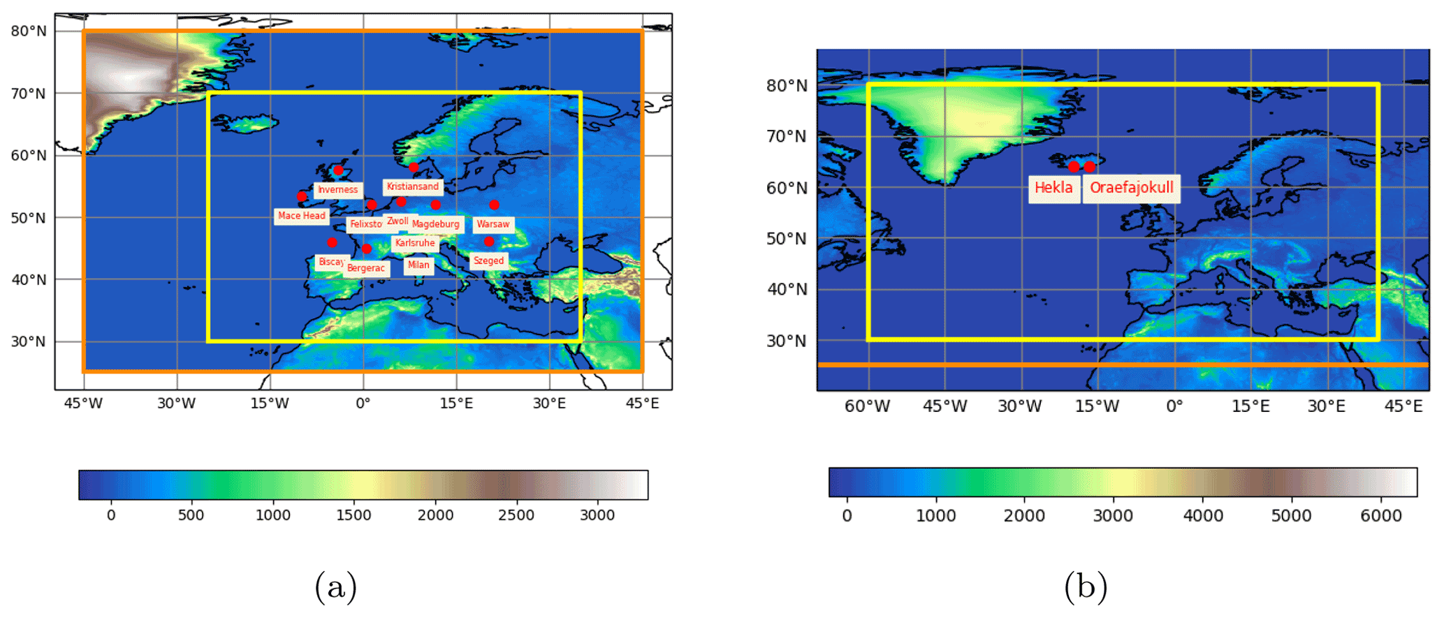
Figure 1Release locations, modelling domain (orange box), and output domain (yellow box) for each scenario. (a) Radiological scenario and (b) volcanic eruption scenario. Note that the modelling domain for the volcanic ash scenario was the whole of the Northern Hemisphere north of 25∘ N.
The first scenario considered a radiological release. Accidental releases from nuclear power plants involve many different radionuclides, but as the aim of this study was to explore meteorological uncertainty rather than source term uncertainty, a hypothetical release of 1 PBq caesium-137 (Cs-137) over 6 h at an elevation of 50 m was used. It was assumed that caesium-137 was carried on particles with a diameter less than 1 µm and had a decay rate of 30 years. To sample a range of different meteorological scenarios, the release was simulated from 12 different locations with different topographical situations and coastal and non-coastal environments across Europe (see Fig. 1a). Note that these locations are not known locations of nuclear facilities: they were just chosen due their topographic and coastal situation. For this scenario, total integrated air concentrations and total deposition were output at the end of a 48 h forecast. Contaminants can remain airborne for longer than 48 h, but the aim of this study was to consider the uncertainty during the initial response to a radiological accident, and this is typically 48 in the UK. In addition, it helped to keep model run times manageable. All quantities were output on a grid with a resolution of 0.141∘ longitude by 0.0943∘ latitude (approximately 10 km by 10 km at mid-latitudes).
The second scenario considered a hypothetical eruption of two volcanoes in Iceland: an eruption of Hekla with an eruption height of 12 km and an eruption of Öraefajökull with an eruption height of 25 km (see Fig. 1b). The runs were set up in the same manner as the operational runs at the London Volcanic Ash Advisory Centre (VAAC) (see Beckett et al., 2020, for more details). Mass eruption rates were computed using a relationship between eruption height and eruption rate proposed by Mastin et al. (2009) and assuming that only 5 % of the ash is small enough to be transported over long distances in the atmosphere. This results in release rates of 8.787×10¹² and 1.131×10¹⁴ g h−1 for Hekla and Öraefajökull respectively. The particle size distribution is based on the eruption of Mount Redoubt in 1990, and particles have a density of 2300 kg m−3. The eruptions were assumed to last for 24 h, and transport and deposition of the emitted ash were modelled for 24 h. The simulations were limited to 24 h, first, because this is the duration of the forecasts VAACs are required to produce and, second, to keep run times manageable. Airborne ash concentrations were output and processed following the same procedure as the London VAAC. First, ash concentrations were averaged over thin layers 25 flight levels (FLs) deep (approximately 800 m), where FLs represent aircraft altitude at standard air pressure and are approximately expressed as hundreds of feet. Then the thin layers were combined into the three thick layers (FL000-200, FL200-350, FL350-550) by taking the maximum ash concentration within the thin layers, which make up a thick layer, and applying it to the entire depth (Webster et al., 2012). In addition, accumulated deposits and 3-hourly vertically integrated ash concentrations (hereafter referred to as ash column load) were also output. All quantities were output on a grid with a resolution of 0.314∘ latitude by 0.179∘ longitude (approximately 20 km by 20 km at mid-latitudes).
To explore a range of meteorological conditions, both scenarios were repeated every 12 h. Computational constraints restricted the period over which runs could be carried out to 4 months between late autumn 2018 and early spring 2019, so runs were carried out for the period 3 November 2018–28 February 2019 for the radiological scenario and 1 December 2018–31 March 2019 for the volcanic eruption scenario, with each simulation being run on a single NWP forecast. Technical issues resulted in the loss of some of the simulations on 18 and 19 January. Therefore a total of 232 simulations of the radiological scenario and 240 simulations of the volcanic eruption scenario were carried out. In both scenarios the release start times are 6 h after the meteorological forecast data initialisation time.
2.1 Overview of NAME
Dispersion modelling was carried out using NAME (Numerical Atmospheric-dispersion Modelling Environment), the UK Met Office's Lagrangian particle dispersion model. NAME is used to model the atmospheric transport and dispersion of a range of gases and particles (Jones et al., 2007). It is the operational model of the London VAAC responsible for forecasting the dispersion of ash in the north-eastern Atlantic and over the UK, Ireland, and Scandinavia, and it is also the operational model of RSMC Exeter (Regional Specialist Meteorological Centre) responsible for forecasting the dispersion of radioactive material in Europe and Africa. In NAME, large numbers of computational particles are released into the model atmosphere, with each computational particle representing a proportion of the mass of the material (gases or particles) being modelled. Computational particles are advected within the model atmosphere by three-dimensional winds from numerical weather prediction models and turbulent dispersion is simulated by random walk techniques. Mass is removed from the model atmosphere by wet and dry deposition as well as by gravitational settling for volcanic ash and by radioactive decay for caesium-137.
2.2 Meteorological data
Meteorological data sets for this study are provided by three different model configurations of the Met Office's Unified Model (Walters et al., 2019). The ensemble meteorological data are provided by the global configuration of the Met Office Global and Regional Ensemble Prediction System (MOGREPS-G), which is an ensemble forecasting system developed and run operationally at the Met Office (Tennant and Beare, 2014). It is an 18-member ensemble which runs four times a day at 00:00, 06:00, 12:00, and 18:00 UTC. In the global configuration it runs at a resolution of 0.28125∘ latitude by 0.1875∘ longitude (approximately 20 km by 20 km at mid-latitudes) with 70 vertical levels extending from the surface up to 80 km (in these simulations only the first 59 levels extending up to 30 km are used). At the time this work was carried out initial conditions were obtained from the global deterministic 4D-Var data assimilation system with perturbations generated using an ensemble transform Kalman filter (ETKF) approach. Model perturbations followed a stochastic physics approach where the tendency of model parameters such as temperature were perturbed. In this configuration MOGREPS-G does not target specific features or geographical areas and it is optimised for error growth at all forecast lead times.
The ensemble dispersion simulations are compared to dispersion runs carried out using the global deterministic configuration of the Met Office Unified Model (hereafter referred to as the deterministic forecast). The global deterministic configuration of the Unified Model (Walters et al., 2019) has a resolution of 0.140625∘ latitude by 0.09375∘ longitude (approximately 10 km by 10 km at mid-latitudes) and has the same vertical level set as MOGREPS-G. It runs four times a day, two 168 h forecasts at 00:00 and 12:00 UTC and two update forecasts of 69 h at 06:00 and 18:00 UTC.
An analysis meteorological data set is constructed by stitching together the first 6 h of each 6-hourly forecast and the dispersion simulations are repeated using this data set. This means that for the first 6 h of meteorological data the deterministic forecast and the analysis meteorology will be identical. Therefore, to avoid giving the deterministic meteorology a skill advantage, the simulated releases are 6 h after the meteorological forecast data initialisation time.
In this study dispersion forecasts are initiated only on the forecasts (ensemble and deterministic) at 00:00 and 12:00 UTC because the data for NAME are only retrieved for the first 6 h of the 69 h update forecasts in order to update the analysis meteorology.
2.3 Assessment of ensemble skill
There are many ways to assess the performance of an ensemble (Wilks, 2019). Some of these measure attributes, such as reliability, which measures the degree to which simulated probabilities match observed frequencies, and resolution that measures the ability of the ensemble to distinguish between events with different frequencies, can only be calculated for a (large) set of ensembles. The aim of this study is to evaluate the skill of each individual simulation, and to do this the Brier score relative to the analysis (Brier, 1950) is used. The Brier score is commonly used to evaluate meteorological ensembles and is completely analogous to the mean-square-error measure of accuracy used for deterministic forecasts. The Brier score is a measure of the accuracy of a forecast in terms of the probability of the occurrence of an event. For a set of N forecasts it is typically expressed as
where fi is the forecast probability of the event occurring for the ith forecast and ai is the observation of the event, with ai=0 if the event does not occur and ai=1 if it does occur. Here the dispersion prediction using the analysis meteorology is substituted for the observation. The Brier score ranges from 0 to 1 and is negatively oriented, so that a perfect forecast is assigned a Brier score of 0. For each scenario an event was considered to have occurred if a threshold concentration (or deposition amount) was exceeded in a single output grid square.
Table 1Thresholds used in the assessment of forecast skill for each of the quantities' output from the radiological and volcanic ash scenarios.
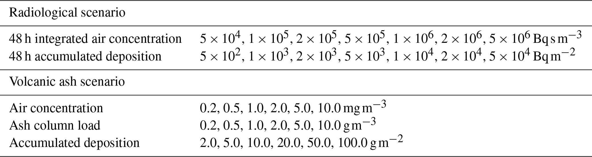
Several thresholds were used for each of the scenarios (see Table 1). The simplification of the release rate for the radiological scenario means that there are no relevant published thresholds. As part of the CONFIDENCE project a hypothetical severe accident was modelled using a range of dispersion models and ensemble meteorology (Korsakissok et al., 2020). A 37 kBq m−2 threshold for deposition of Cs-137 was exceeded at distances of 100–200 km from the release location. Here thresholds for the radiological scenario were chosen so that the highest thresholds were exceeded at 100–200 km from the release location and with the remaining thresholds were selected on an decreasing log scale. Average (mean) maximum distances at which thresholds are exceeded are calculated by computing the maximum distance at which each threshold is exceeded for every location, every ensemble member, and every simulation and then averaging over the ensemble members and simulations.
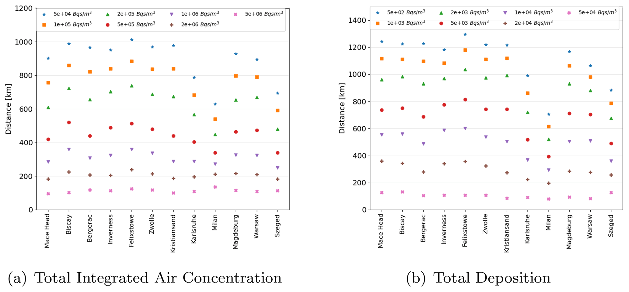
Figure 2Average maximum distances at which thresholds are exceeded for (a) total integrated air activity of Cs-137 and (b) total accumulated deposits of Cs-137 for each of the 12 release locations and each of the six thresholds.
It can be seen from the average maximum distance from the release location that the highest threshold is exceeded is around 100 km for all of the release locations (see Fig. 2). The average maximum distance that the lowest threshold is exceeded is between approximately 650 and 1000 km from the release location for the total integrated air concentration and between approximately 700 and 1300 km from the release location for the accumulated deposition. The average maximum distances at which thresholds were exceeded are lowest for the releases from Milan, Italy, and highest for the releases from Felixstowe, UK, reflecting the different weather patterns that influence these locations. Milan, Italy, is surrounded by the Alps on the northern and western sides and so is sheltered from the westerly and southwesterly prevailing winds. In contrast, Felixstowe is in a low-lying region of the UK with no shelter from the prevailing westerly and southwesterly winds, and the prevailing winds carry material across the sea, where winds speeds are typically higher than over land.
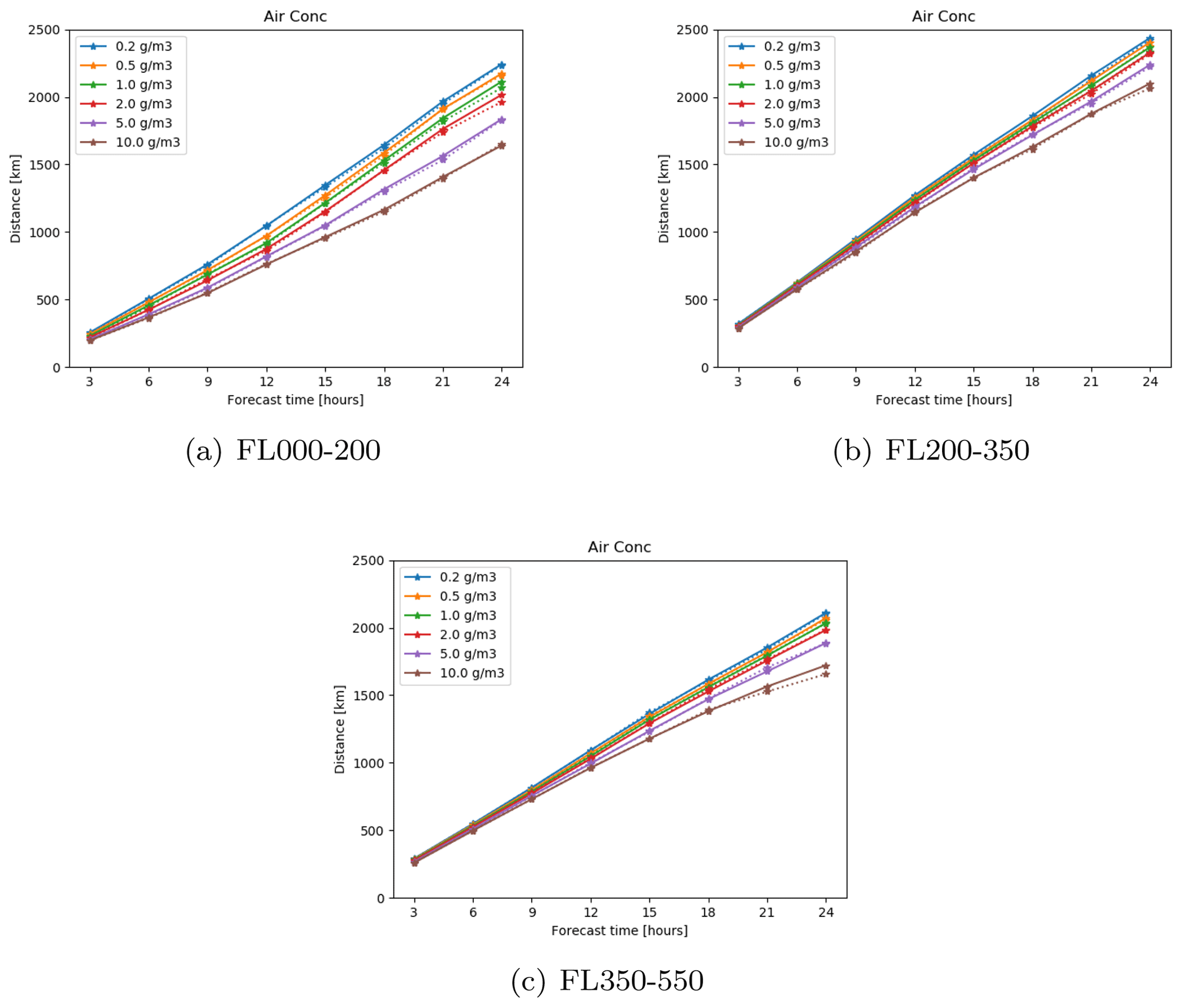
Figure 3Average maximum distances at which thresholds are exceeded for air concentrations on (a) FL000-200, (b) FL200-350, and (c) FL350-550 for each of the six thresholds. The solid line represents average maximum distances from ensemble simulations and the dotted line represents average maximum distances from the analysis simulations of the Hekla scenario.
Thresholds for the volcanic ash scenario air concentration values reflect values discussed in the literature. The London VAAC currently uses thresholds of 0.2, 2.0, and 4.0 mg m−3 (Beckett et al., 2020). Prata et al. (2019) note that thresholds between 2.0 and 10.0 mg m−3 have been discussed in meetings with aviation stakeholders, and studies of engine damage consider damage against a log scale of air concentration (Clarkson and Simpson, 2017). Therefore, the thresholds for air concentration of volcanic ash used in this study range from 0.2 to 10.0 mg m−3 on a log scale. Threshold concentrations for ash column load assume that layers of volcanic ash are on average 1 km thick and so are chosen to be a factor of 1000 larger than the thresholds for air concentration. Accumulated deposition thresholds were chosen so that the areas where deposition exceeded the thresholds were similar to the areas where the air concentration exceeded the thresholds. Average maximum distances at which thresholds are exceeded for each of the three flight levels for the Hekla scenario are shown in Fig. 3. As expected, the average maximum distance at which the thresholds are exceeded increases over time; 3 h after the start of the eruption all of the thresholds are exceeded to a maximum distance of around 250 km at all three flight levels; 24 h after the start of the eruption the average maximum distance over which thresholds are exceeded ranges from approximately 1600 to 2400 km. To provide a sense of scale 1600 km is the approximate distance from Reykjavik, Iceland, to Bern, Switzerland. The smallest distances are for the highest thresholds in FL000-200 and FL350-550 and the largest distances are for the lowest thresholds in FL200-250.
The Brier score is often compared to a reference Brier score to produce a Brier skill score. In meteorology the most commonly used reference is climatology. However, there is no climatology for a single release dispersion event, so instead a reference forecast is used. In this case the forecast using the global Unified Model is used as a reference as it also demonstrates whether or not the ensemble forecast outperforms the deterministic forecast. This is not perfect because the deterministic and analysis meteorology has the same resolution, while the ensemble meteorology has a coarser resolution. However, all three meteorological configurations are initialised using the same observations, and the models would be used in their native resolution in a real dispersion incident, so this provides an indication of the models' performance in that they would be used in real incidents. The Brier skill score is expressed as
In this case the Brier skill score indicates the level of performance of the ensemble over the deterministic forecast, so ensemble forecasts that outperform their deterministic counterparts have positive Brier skill scores and ensemble forecasts that perform worse than their deterministic counterparts have negative Brier skill scores. It provides an indication of the relative performance of the ensemble and deterministic forecasts rather than an measure of absolute performance, so that if the deterministic and ensemble forecasts both perform well but the deterministic performs slightly better, the ensemble forecast will have a negative Brier skill score.
The Brier skill score can range from −∞ to +1, so average Brier skill scores are computed by first computing the average Brier scores for the ensemble and the deterministic meteorology and then using Eq. (2) to compute the average Brier skill score.
In this section, the Brier skill scores for the ensemble runs are presented. First the average Brier skill scores are presented for each scenario and each release location. Then a few simulations where the skill score was high or low are examined to provide examples of the situations where simulations using ensemble meteorology outperform those using deterministic meteorology and vice versa. It should be noted that the Brier skill scores only provide an assessment of the relative performance of the ensemble forecast when compared to the deterministic forecast rather than an absolute measure of the performance of the ensemble forecast.
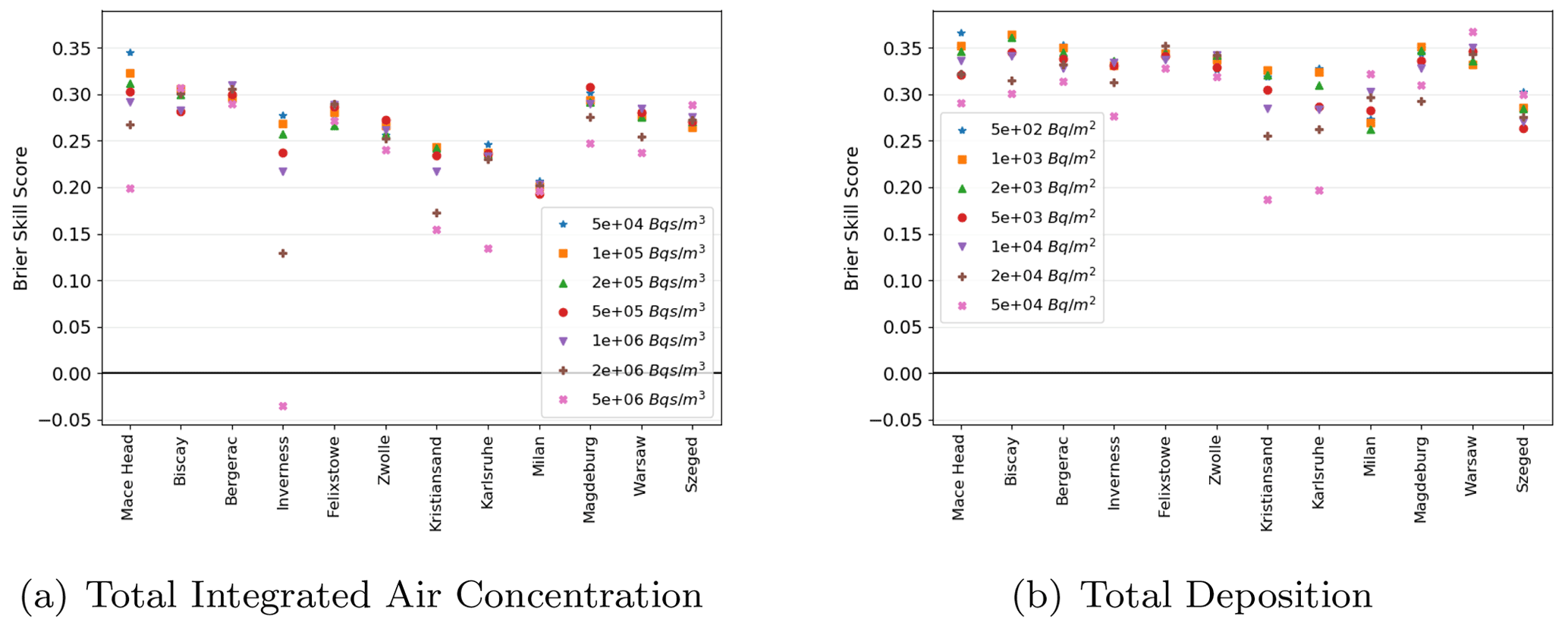
Figure 4Average Brier skill score for (a) total integrated air activity of Cs-137 and (b) total accumulated deposits of Cs-137 for each of the 12 release locations and each of the six thresholds.
3.1 Radiological scenario
Figure 4 shows the average Brier skill score at each of the 12 locations where a hypothetical radiological release was simulated. Seven threshold values are shown for each of the 48 h integrated air concentrations and the 48 h accumulated deposition. Average skill scores are higher for the accumulated deposition than the air concentration and there is more variation in skill score between the different locations for the accumulated air concentration. The highest average skill scores are at Mace Head and the lowest skill scores at the lower threshold values can be found at Milan. However, there is a greater range of skill scores between the thresholds at Inverness, and the average skill score for the highest threshold is negative, implying that for this threshold, on average, the dispersion runs using deterministic meteorology performed better than the dispersion runs using ensemble meteorology. For the accumulated air concentration the lowest skill scores were seen for the highest threshold at 8 out of the 12 release locations. This is typically because the highest thresholds are exceeded close to the release location and soon after the release time when the ensemble performs less well than the deterministic simulations (not shown). The same was true for the accumulated deposition, although for a different set of eight release locations.
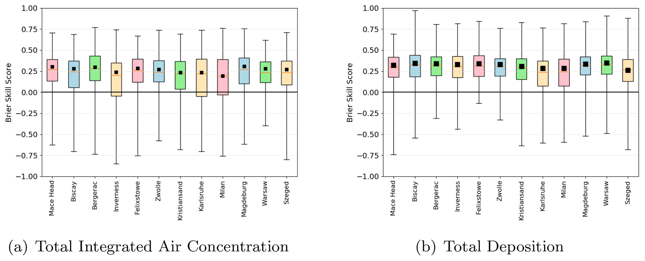
Figure 5Adjusted Brier skill score for (a) total integrated air activity of Cs-137 above 50 kBq s m−3 and (b) total accumulated deposits of Cs-137 above 5 kBq m−2 for each of the 12 release locations. Black squares show average Brier skill scores at each location and the box and whiskers show the range of adjusted skill scores for each individual simulation.
Although the average Brier skill score at each location is positive, implying that on average the ensemble performs better than the deterministic simulation, there are simulations at all locations for which the skill score is negative (Fig. 5). The standard Brier skill score can take any value from −∞ to 1, but this means that it is difficult to assess the relative size of negative and positive Brier skill scores on a single plot. Therefore, in Fig. 5 the Brier skill score has been adjusted, so that negative Brier skill scores lie in the range . This adjusted score is defined as
For the thresholds shown in Fig. 5 Brier skill scores are negative for between 10 % and 30 % of the simulations of total accumulated air concentration and between 0.5 % and 19 % of the simulations of accumulated deposition. The highest percentages of negative skill scores are from the simulations of releases at Karlsruhe and Milan for integrated air concentration and deposition respectively, and the lowest percentages of negative skill scores are from the simulations of releases at Warsaw for both integrated air concentration and deposition. Generally simulations from release locations with a larger percentage of negative skill scores for integrated air concentration also have a larger percentage of negative skill scores for deposition.
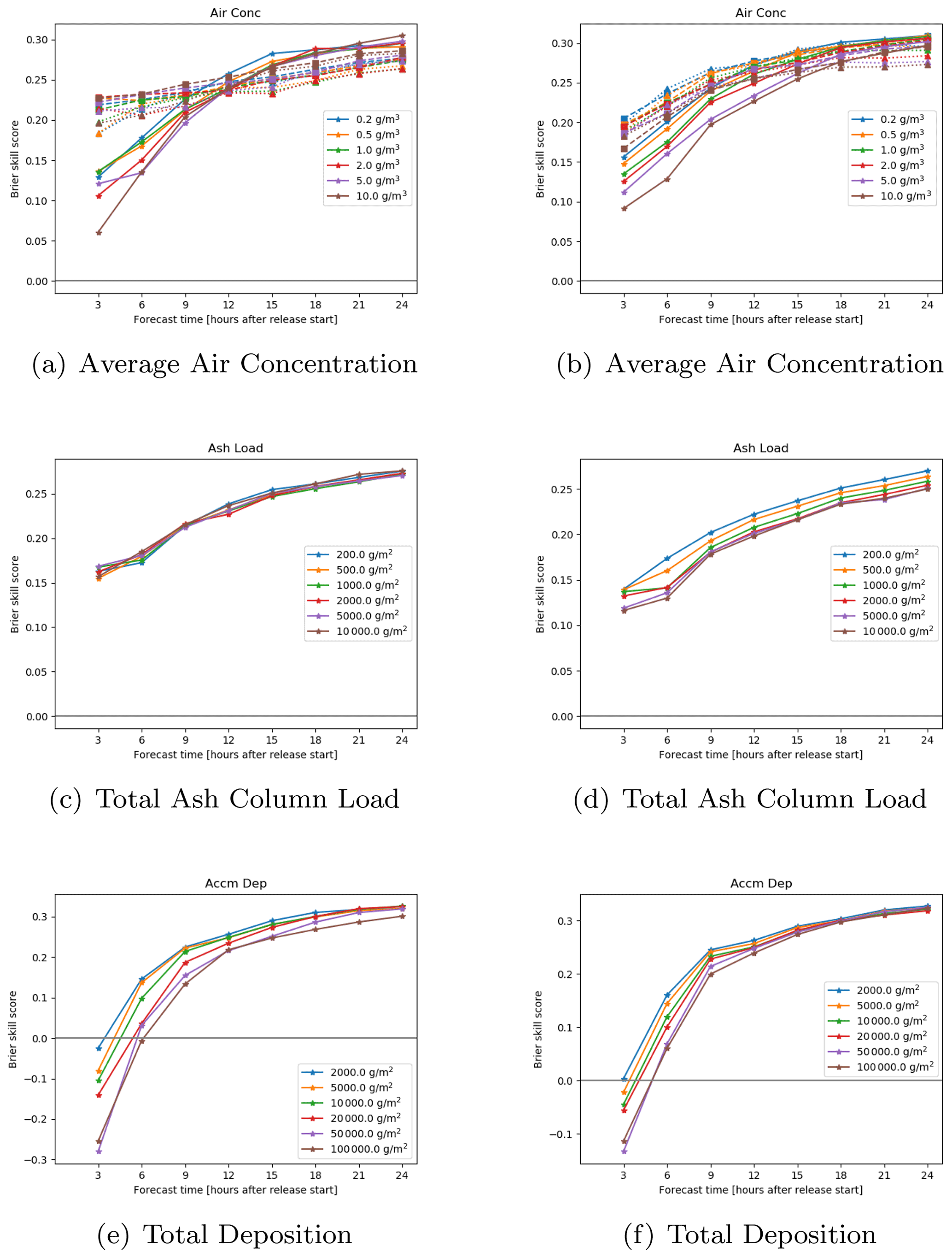
Figure 6Brier skill score against forecast time (hours since the start of the eruption) for (a, b) ash concentration on three flight levels (solid lines are FL000-200, dashed lines are FL200-350, and dotted lines are FL350-550), (c, d) ash column load, and (e, f) accumulated deposition for five different thresholds. The left-hand-side column is for a 12 km eruption of Hekla and the right-hand-side column is for a 25 km eruption of Öraefajökull.
3.2 Volcanic ash scenario
For the volcanic ash scenarios Brier skill scores were computed for the air concentration on three flight levels, FL000-200, FL200-350, and FL350-550, the air concentration integrated over the whole depth of the model atmosphere (the ash column load) and the accumulated deposits. Average unadjusted Brier skill scores are shown in Fig. 6, and it can be seen that after the first time step the average scores are greater than zero, suggesting that on average the ensemble outperforms the deterministic forecast. Brier skill scores increase with forecast time, and the increase is fastest for the accumulated deposition and slowest for the highest flight level (FL350-550) for the 12 km eruption scenario. Generally, average skill scores are higher for smaller thresholds, although the difference in skill score between the thresholds is smaller than the difference in the skill scores between the forecast times. With the exception of the upper two flight levels, skill scores are similar for the 12 km eruption scenario and the 25 km eruption scenario. The 12 km eruption will only emit a small amount of material into the highest flight level, FL350-550, because FL350 is typically around 11 km above sea level.

Figure 7Adjusted Brier skill score against forecast time for ash concentration exceeding 5 mg m−3 on three flight levels: (a) Fl000-200, (b) FL200-350, and (c) FL350-550. The left-hand-side column is for a 12 km eruption of Hekla and the right-hand-side column is for a 25 km eruption of Öraefajökull. Black squares show average Brier skill scores and the box and whiskers show the range of adjusted skill scores for each individual simulation.
Although the average Brier skill scores are generally greater than zero, at each forecast time step there are runs where the Brier skill score is negative, suggesting that the deterministic forecast outperforms the ensemble (see Fig. 7, which shows individual adjusted Brier scores). At later forecast time steps there are fewer negative scoring runs, and the range of Brier skill scores is narrower. The reduction in negative scoring runs implies that the ensemble is more likely to perform better than the deterministic one at later time steps. This is possibly due to the increase in ensemble spread at later time steps. The reduction in the range of the Brier skill scores is likely to be due to the increase in area exceeding the threshold. At early time steps when the plume is narrow, the Brier skill score is dominated by a few grid cells and the ensemble tends to be less spread, resulting in either a high Brier skill score or a very low Brier skill score. At later time steps the plume is more spread out and the ensemble is more spread, so there is a greater range of Brier scores for the different grid cells and the Brier skill score tends to be closer to zero.
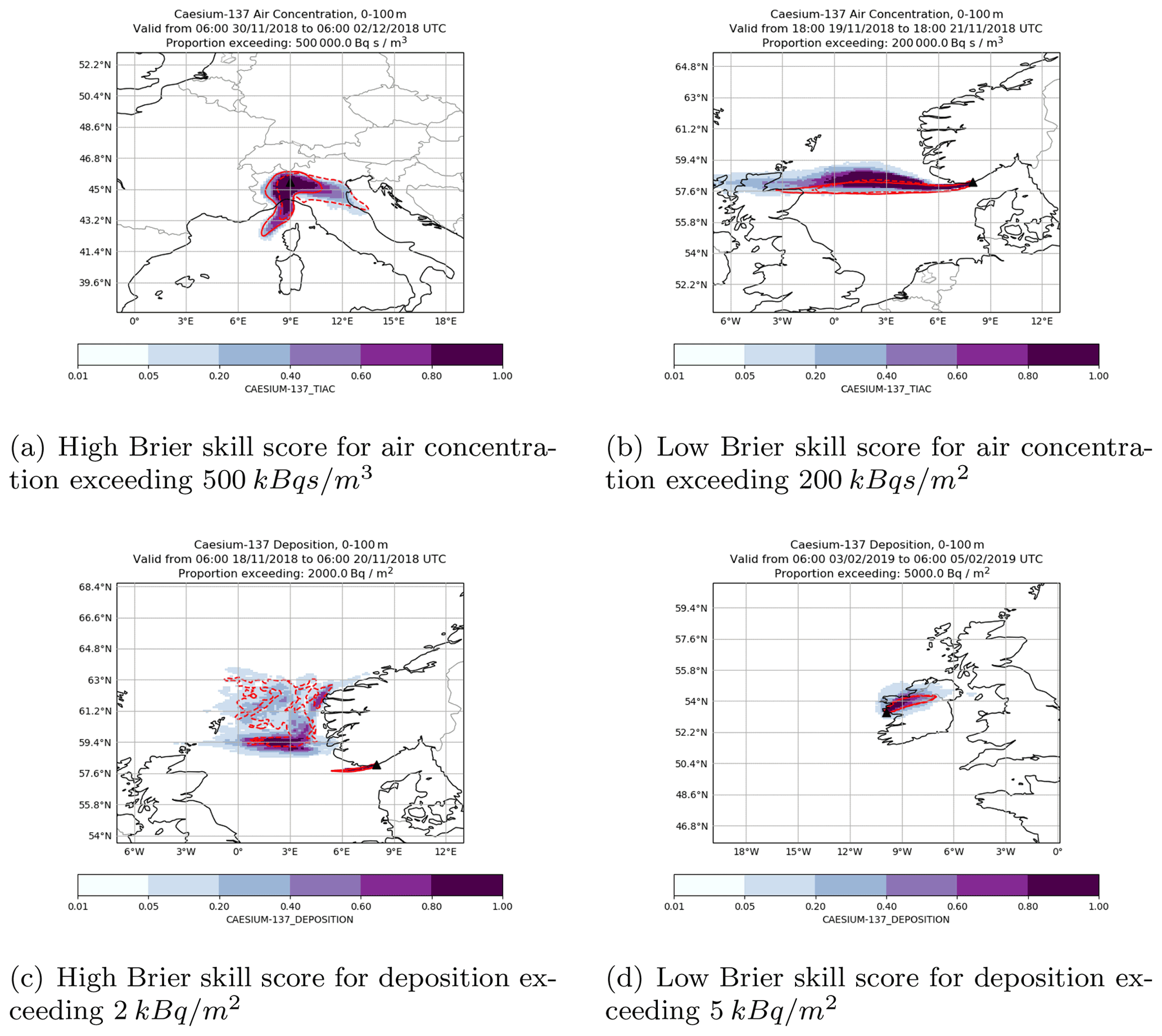
Figure 8Examples of high and low Brier skill scores from the radiological scenario. The coloured contours show the probability of the ensemble predictions exceeding the threshold. The area where the threshold is exceeded by the analysis simulation is shown by a red solid line and the area where the threshold is exceeded for the deterministic simulation by a red dashed line.
3.3 Examples of high and low Brier skill scores
The Brier skill score is a statistical method of quantifying the performance of an ensemble of predictions against a reference prediction. However, it hides a lot of detail. In this section examples of simulations where the Brier skill score is high and low are examined in more detail. Examples of high and low Brier skill score were selected from the radiological scenario by considering predictions where the adjusted Brier skill score was greater than 0.6 or less than −0.6 for four or more thresholds for a single simulation. The subset of examples in Fig. 8 was then randomly selected from the simulations fitting these criteria.
Figure 8a shows an example of a high Brier skill score for a prediction of integrated air concentration following a hypothetical release from Milan in northern Italy. In this example the deterministic simulation predicted some transport to the south-west and a large amount of transport to the south-east, broadly following the Po Valley. In contrast, the analysis simulation predicted a small amount of transport to the south-east and a greater amount of transport to the south-west. The ensemble simulation spans both of these predictions, and the area where more than 60 % of ensemble members exceed the threshold extends a similar distance in the south-westerly and south-easterly directions. This resulted in a Brier skill score of 0.76.
Figure 8b shows an example of a low Brier skill score for a prediction of air concentration following a hypothetical release from Kristiansand. In this example the region where the threshold is predicted to be above 200 kBq s m−3 is very similar in the deterministic and analysis runs, extending due west from the release site. In contrast, most ensemble members predict that the threshold will be exceeded in a region slightly further north. At the time of this release a high-pressure system was located over Norway and a low-pressure system was located to the south of Greenland. This resulted in a high gradient of wind speed and a change in wind direction close to Kristiansand (see Fig. 9a). At the start of the release wind speeds at Kristiansand were greater in all the ensemble members than both the deterministic and analysis meteorological data, and wind directions were more easterly and less southerly in all the ensemble members than both the deterministic and analysis meteorological data (see Fig. 9b and c). This suggests that the location of the highest gradient in wind speed and change in wind direction were slightly different in all ensemble members, resulting in the different predictions of air concentration.
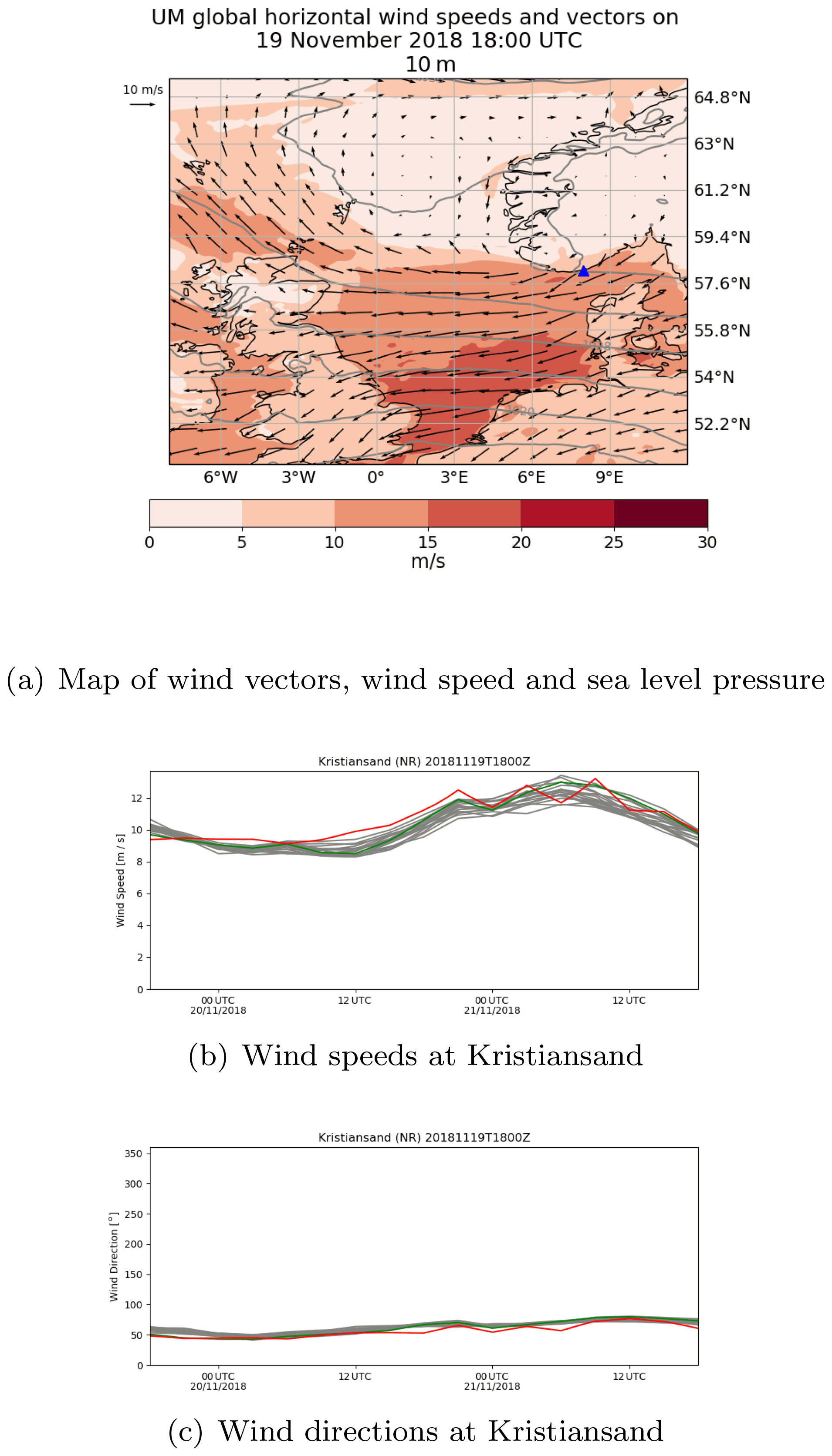
Figure 9(a) Map of 10 m wind vectors (arrows), 10 m wind speed (red shading), and sea level pressure (grey lines) from the analysis meteorological data set at 18:00 UTC on 19 November 2018. Kristiansand (Norway) is marked with a blue triangle. (b) 10 m wind speed and (c) 10 m wind direction at Kristiansand (Norway) from the ensemble forecast (grey lines), deterministic forecast (green line), and analysis meteorology (red line).
Figure 8c shows an example of a high Brier skill score for a prediction of accumulated deposition following a hypothetical release from Kristiansand. The area where the deposits exceed 2 kBq m−2 is complex because the deposition is dominated by wet deposition. The area exceeding the threshold predicted by the deterministic simulation covers a large area of the North Sea between the Norwegian coast and the Shetland Islands. However, the area exceeding the threshold in the analysis simulation is mostly limited to a narrow region immediately to the west of the release site. There are three regions where more than 60 % of ensemble members are in agreement so that the threshold will be exceeded: one in the narrow region immediately to the west of the release site, one extending from 0 to 4∘ E at 59.4∘ N, and one close to the western-most point of the Norwegian coast. Both the ensemble and the deterministic simulation show relatively poor agreement with the analysis simulation but, because, in most areas, only a small proportion of the ensemble exceeds the threshold, it has a lower Brier score than the deterministic one, and thus the Brier skill score is positive.
Figure 8d shows an example of a low Brier skill score for a prediction of accumulated deposition following a hypothetical release from Mace Head in Ireland. In this case the area where deposits are predicted to exceed 5 kBq m−2 is similar in the analysis and deterministic simulations. Although this region closely matches the region where 60 % of the ensemble members exceed the same threshold, the good agreement between the analysis and the deterministic simulations coupled with a few ensemble members predicting the threshold will be exceeded further to the north results in a lower Brier score for the deterministic than for the ensemble simulations. This is an example of a case where the ensemble forecast is unable to show an improvement in the deterministic forecast because the deterministic forecast performs highly. The negative Brier skill score only provides a comparison of the performance of the ensemble relative to the deterministic one and does not provide information about the individual performance of the ensemble.
For the volcanic ash scenario, Brier skill scores were closer to zero, so examples of high and low Brier skill scores were selected by considering all simulations where the adjusted skill score was greater than 0.5 or less than −0.5 for at least two time steps at a single flight level. Examples were randomly chosen from the simulations meeting these criteria.
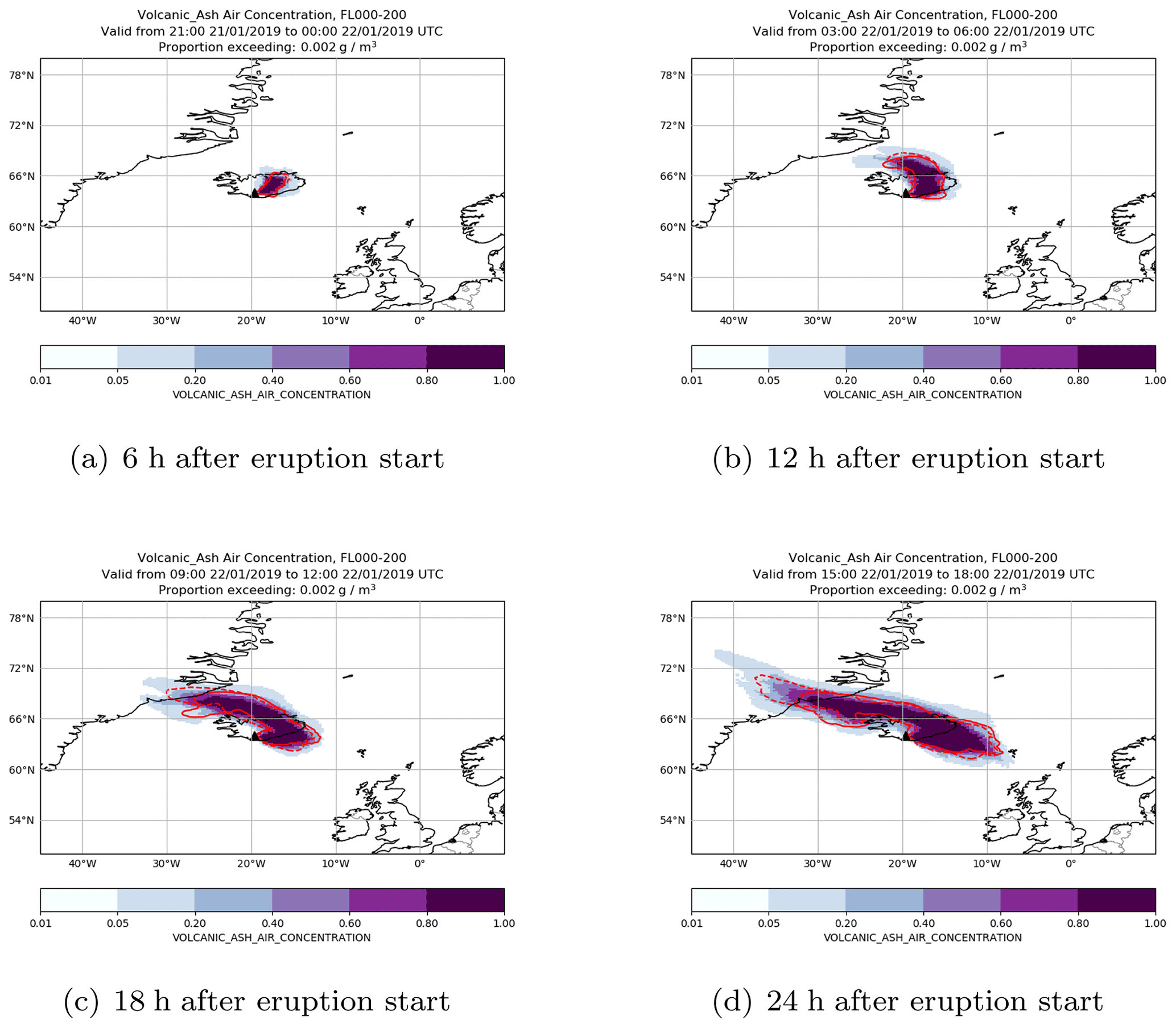
Figure 10A volcanic ash simulation of Hekla where the Brier skill score is high for concentrations exceeding 2 mg m−3 at FL000-200. The coloured contours show the probability of the ensemble predictions exceeding the threshold in 6 h time steps starting 6 h after the eruption. The area where the threshold is exceeded by the analysis simulation is shown by a red solid line and the area where the threshold is exceeded for the deterministic simulation by a red dashed line.
Figure 10 shows an example of a simulation where the Brier skill score is positive, implying that the ensemble simulation performs better than the single deterministic simulation. The simulation considers a hypothetical volcanic eruption at Hekla with an eruption height of 12 km starting at 18:00 UTC on 21 January 2019. Figure 10 shows regions where the air concentration in FL000-200 exceeds 2 mg m−3. Volcanic ash is initially transported in a north-easterly direction; 6 h after the start of the eruption material to the north of Iceland is transported to the north-west, while newly emitted material is transported to the south-east, resulting in a bi-directional plume extending in the north-westerly and south-easterly directions from the volcano.
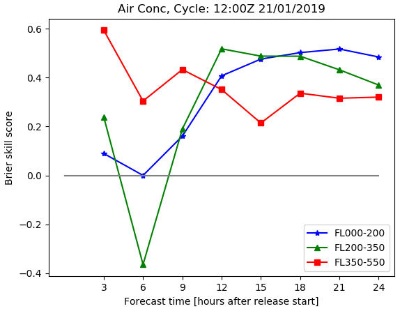
Figure 11Brier skill score changes with time since the start of the eruption for a simulation with a high Brier score. This is for the same case as Fig. 10.
The Brier skill score for this simulation is positive for all flight levels and all time steps except 6 h after the eruption, where there are negative and zero skill scores for concentrations exceeding 2 mg m−3 at heights of FL200-350 and FL000-200 respectively (see Fig. 11). The skill score for the lowest flight level gradually increases from 6 h after the eruption to 21 h after the eruption before decreasing slightly. In the middle flight level a similar pattern is observed, although in this case the highest skill score occurs 9 h after the eruption, and at the highest flight level there is a slight downward trend in the skill score over time. This demonstrates how ensemble skill, relative to deterministic simulation skill, can vary with height.
What do these Brier skill scores mean for the difference between the ensemble, deterministic, and analysis simulations for the concentration of ash exceeding 2 mg m−3 at FL000-200? Six hours after the start of the eruption there is good agreement between the deterministic and analysis simulations, but there are a few members of the ensemble simulation predicting greater plume spread in an east–west direction. This is consistent with a Brier skill score close to zero. Twelve hours after the start of the eruption the deterministic and analysis simulations start to diverge, particularly at the north-western end of the plume, and 24 h after the start of the eruption the analysis simulation predicts that the plume will just reach the coast of Greenland, but the deterministic simulation predicts that the plume will extend approximately 5∘ further west. A few ensemble members also predict that the plume will extend several degrees to the west of the coast of Greenland. However, the region where all ensemble members are in agreement that the air concentration will exceed a threshold of 2 mg m−3 is in good agreement with the region where the analysis simulation exceeds the same threshold. The Brier skill scores for 12, 18, and 24 h after the start of the eruption are 0.407, 0.502, and 0.484 respectively, indicating that during this time period the ensemble outperforms the deterministic simulation.
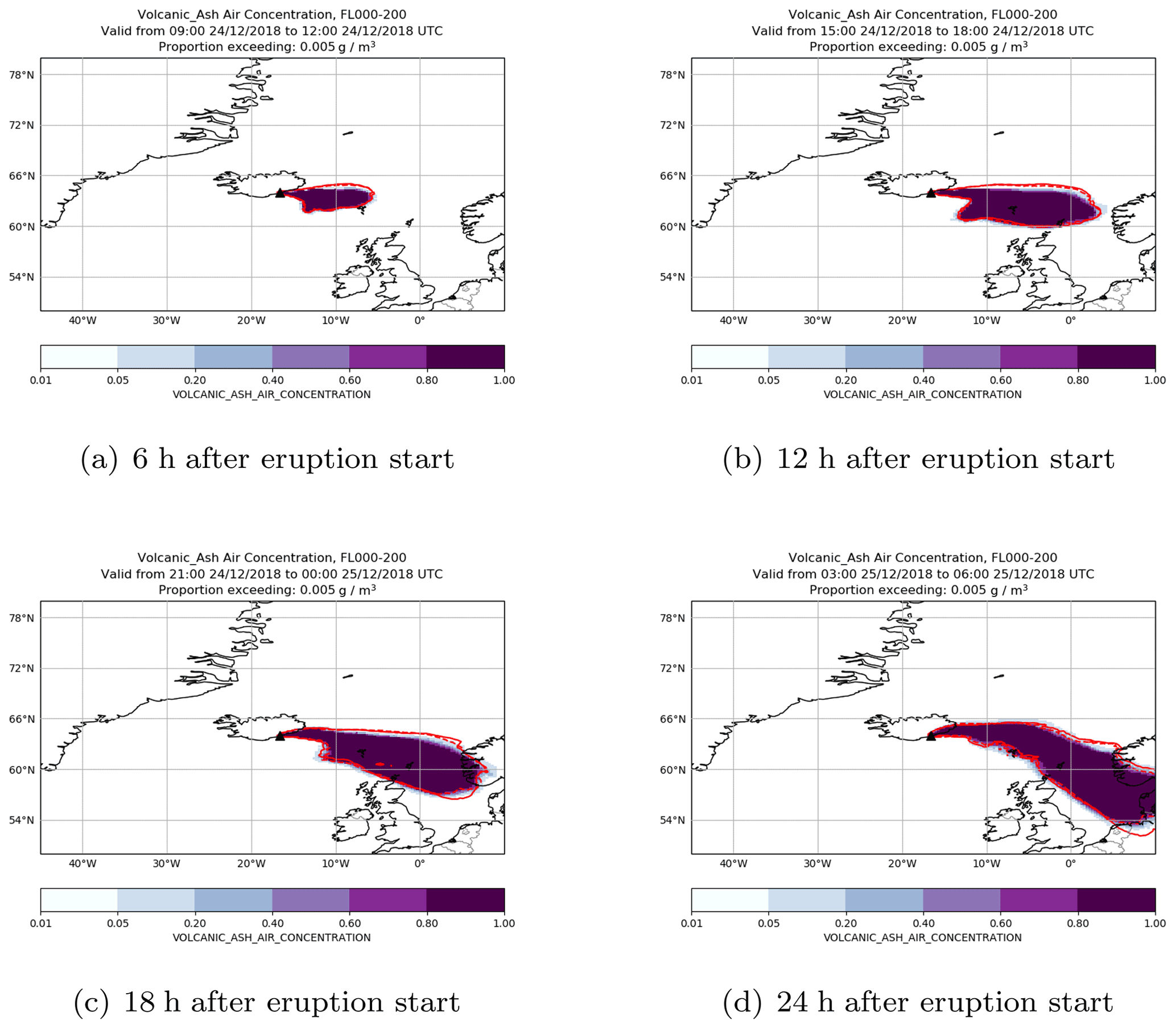
Figure 12A volcanic ash simulation of Öraefajökull where the Brier skill score is low for concentrations exceeding 5 mg m−3 at FL000-200. The coloured contours show the probability of the ensemble predictions exceeding the threshold in 6 h time steps starting 6 h after the eruption. The area where the threshold is exceeded by the analysis simulation is shown by a red solid line and the area where the threshold is exceeded for the deterministic simulation by a red dashed line.
Figure 12 shows an example of a volcanic ash simulation where the Brier skill score is negative, implying that the deterministic simulation outperforms the ensemble simulation. This simulation considers a hypothetical eruption of Öraefajökull with an eruption height of 25 km starting at 06:00 UTC on 24 December 2018. Material in the lowest flight level (FL000-200) is transported eastwards from Iceland. There is also some southward transport of the ash to the east of Iceland, and this increases with each time step so that the region exceeding 5 mg m−3 extends down the North Sea across the Shetland Islands, the southern and western coasts of Norway, and much of Denmark.
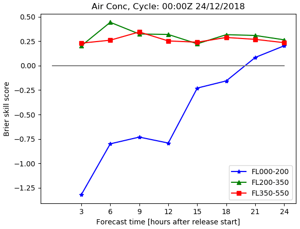
Figure 13Brier skill score changes over time since the start of the eruption for a simulation with a low Brier score. This is for the same case as Fig. 12.
The Brier skill score for ash concentrations exceeding 5 mg m−3 in the upper two flight levels, FL200-350 and FL350-550, for this simulation are both positive and change little over the duration of the simulation (see Fig. 13). However, at the lowest flight level, FL000-200, the skill score for ash concentrations exceeding 5 mg m−3 is initially very negative and then gradually increases over time, becoming positive 21 h after the eruption.
At the lowest flight level, there is good agreement between the regions where the ash concentration is predicted to exceed 5 mg m−3 in the deterministic and analysis runs. In addition, there is very little spread in the ensemble, and the region where 80 % of ensemble members predict volcanic ash concentrations to exceed the threshold closely matches the region of threshold exceedance from the analysis simulation. There is a small mismatch on the northern edge of the region, where 80 % of ensemble members predict concentrations above the threshold and where the analysis and deterministic simulations predict concentrations above the threshold, and this results in a negative Brier skill score.
In this section six example simulations have been considered, three where the Brier skill score had a large positive value and three where the skill score had a large negative value. The large positive values can be attributed to simulations where the deterministic simulation performed poorly compared to the analysis and the region where the ensemble predicted the highest probabilities of exceeding a threshold compared well to the analysis simulation. The large negative values occurred in simulations where the deterministic simulation performed well compared to the analysis. In this case the ensembles demonstrated different behaviour: in one case the ensemble predicted transport in a different direction to the analysis, in the second case there was some spread in the ensemble, and in the final case there was very little spread in the ensemble.
This study considers how well a dispersion ensemble constructed using input from a meteorological ensemble model might be expected to perform when compared to a dispersion model using single-model deterministic meteorology. Meteorology from the Met Office MOGREPS-G ensemble prediction system is used as input to the NAME dispersion model generating an 18-member dispersion ensemble. The dispersion output is then compared to runs using forecast meteorology from the global deterministic configuration of the Met Office Unified model (referred to as deterministic meteorology). To provide a “ground truth” an analysis meteorological data set is constructed by stitching together the first 6 h of each 6-hourly deterministic meteorological forecast.
Dispersion output from two hypothetical scenarios is explored: the first scenario is a near-surface release of radioactive material and the second scenario is a volcanic eruption in Iceland. Simulations of both scenarios are repeated over a 4-month period to sample a range of meteorological conditions. Two volcanic eruptions are considered, a 12 km eruption of Hekla lasting 24 h and a 25 km eruption of Öraefajökull also lasting 24 h. To sample different topographical locations, 12 different release sites in Europe are considered for the radiological release, and in each case the release is assumed to last 6 h. For the radiological release scenario total integrated air concentration and total deposition are output after 48 h. For the volcanic eruption scenario air concentrations of volcanic ash on three vertical levels, deposits of volcanic ash and the total column load of volcanic ash are output every 3 h. Outputs from the simulations using ensemble meteorology are compared to the outputs from the simulation using deterministic meteorology using the Brier skill score computed for a range of thresholds.
The results showed that on average Brier skill scores were greater than zero for all release locations for the total integrated air concentration and total deposition from the radiological scenarios. This suggests that on average the ensemble dispersion simulation performed better than the deterministic dispersion simulations. Skill scores were greater than zero for all thresholds except the highest threshold for one release site. Skill scores were slightly higher for total deposition than total integrated air concentration. This may be because predictions of precipitation, and therefore predictions of wet deposition are typically more uncertain than predictions of wind speed and direction, giving the ensemble more scope to add value. It also demonstrates that the value of ensemble forecast data depends on the meteorological parameters that have the greatest influence on the output.
Skill scores for the air concentration, deposition, and total column load of volcanic ash were greater than zero except at 3 h after the start of the eruption, where the skill scores for deposition were negative. Zidikheri et al. (2018) used the Brier skill score to compare ensemble simulations of the eruptions of Rinjani and Kelut to satellite observations. Although this study is not directly comparable because model simulations using deterministic meteorology are used in place of observations, the Brier skill scores are in good agreement. The skill scores increased with time since the start of the eruption, suggesting that the skill of the ensemble increases over time compared to the deterministic simulations. Similar results are observed when the skill of ensemble NWP models is assessed. Examination of individual simulations showed that different skill scores could be obtained for different flight levels so that it was possible for the ensemble to outperform the deterministic one at one flight level but not at the neighbouring flight level.
Two very different scenarios have been considered, the 48 h integrated concentrations resulting from a boundary layer release and the time-varying concentrations resulting from a vertical column release over depths of 12 and 25 km. Average Brier skill scores were greater than zero for both scenarios and for all outputs considered, suggesting that using ensemble meteorology provides value for a wide range of dispersion scenarios. Brier skill scores tend to be slightly greater for the boundary layer scenario, but further work would be needed to determine whether this was due to the height of the release, the averaging period, or the threshold values.
Due to computational constraints this study was only able to examine skill scores over a 4-month period from the end of the Northern Hemisphere autumn to the beginning of spring. This was partially mitigated against for the radiological scenario by using a range of release locations. However, further work would need to be carried out to demonstrate that the results hold for the Northern Hemisphere summer.
In this study, individual ensemble simulations were compared to analysis simulations to assess whether they outperformed forecast simulations. Using this method uncertainty in the source term and the dispersion model parameterisations is excluded. The results could, therefore, be viewed as assessing the performance of the NWP ensemble for dispersion applications; i.e. the study assesses the NWP parameters of importance to dispersion over scales that are important to dispersion. The data set could also be used to assess whether the dispersion ensemble is reliable. That is, the model-predicted probability of an event matches the observed frequency of the same event and has good resolution; i.e. the model is able to distinguish between events which occur with different frequencies. Work to assess this and to increase the range of metrics used to assess the performance of the ensemble is ongoing and will be addressed in a separate paper.
It would also be useful to determine whether there were certain meteorological regimes where ensemble simulations added more value. Meteorological data are often categorised into weather patterns in order to provide a broad overview of future weather as well as a tool to understand the performance of numerical weather prediction (NWP) models. A comparison of the skill of the ensemble within different weather regimes may indicate the weather patterns where ensemble simulations are most likely to add value. However, to sample a range of regimes simulations would need to be carried out over a long period of time. In addition, weather patterns are generally applied to broad areas, whereas the results of this study have demonstrated that skill can vary over much smaller horizontal and vertical extents. Therefore, it may be more helpful and appropriate to compare ensemble performance to measures of the NWP performance or spread over much smaller regions.
The aim of this study was to examine the ability of ensemble meteorology to produce more skillful dispersion output than deterministic meteorology. The study compares ensemble simulations of hypothetical releases to the same simulations carried out with analysis meteorology. Uncertainty in the source term, e.g. release rate, timing, height, and composition, and model parameterisations are ignored. Therefore, the performance of the ensemble seen here may not be reflective of the performance of the ensemble in simulating a real release which would be compared to observations. However, the results do show that on average the ensemble dispersion model outperforms the deterministic model when only meteorology is considered, providing confidence in the use of ensemble meteorology to provide meteorological uncertainty information to dispersion models. As noted in the introduction, the quantification of uncertainty in dispersion model predictions is important in the decision-making process, and this study takes the first steps towards demonstrating the value of ensemble dispersion model predictions.
All the code used within this paper, the dispersion model NAME, the statistical calculation code, and the plotting code is available under licence from the Met Office. For access, please contact the authors. The meteorological data used to drive the dispersion model were not generated by this project and are not archived due to the huge volumes involved. Data produced during this work, output from the dispersion model, and the results of the statistical calculations are available via Zenodo at https://doi.org/10.5281/zenodo.4770066 (Leadbetter and Jones, 2021).
The project was conceptualised by ARJ and SJL. Formal analysis was carried out by SJL and ARJ. The original draft was written by SJL and SJL, ARJ and MCH contributed to the discussion of the results and the revision of the draft.
The contact author has declared that neither they nor their co-authors have any competing interests.
Publisher's note: Copernicus Publications remains neutral with regard to jurisdictional claims in published maps and institutional affiliations.
The authors would like to thank Frances Beckett and Nina Kristiansen (ADAQ, Met Office) for their advice on the volcanic scenario set-up and Sarah Millington (ADAQ, Met Office) for her review of a draft of the manuscript.
This paper was edited by Anja Schmidt and reviewed by three anonymous referees.
Beckett, F. M., Witham, C. S., Leadbetter, S. J., Crocker, R., Webster, H. N., Hort, M. C., Jones, A. R., Devenish, B. J., and Thomson, D. J.: Atmospheric dispersion modelling at the London VAAC: A review of developments since the 2010 eyjafjallajökull volcano ash cloud, Atmosphere, 11, 352, https://doi.org/10.3390/atmos11040352, 2020. a, b, c
Bowler, N. E., Cullen, M. J. P., and Piccolo, C.: Verification against perturbed analyses and observations, Nonlin. Processes Geophys., 22, 403–411, https://doi.org/10.5194/npg-22-403-2015, 2015. a
Brier, G. W.: Verification of forecasts expressed in terms of probability, Mon. Weather Rev., 78, 1–3, https://doi.org/10.1175/1520-0493(1950)078<0001:VOFEIT>2.0.CO;2, 1950. a
Clarkson, R. and Simpson, H.: Maximising Airspace Use During Volcanic Eruptions: Matching Engine Durability against Ash Cloud Occurrence, NATO unclassified, available at: https://www.sto.nato.int/publications/STO%20Meeting%20Proceedings/STO-MP-AVT-272/MP-AVT-272-17.pdf (last access: 12 January 2022), 2017. a
Dacre, H. F. and Harvey, N. J.: Characterizing the atmospheric conditions leading to large error growth in volcanic ash cloud forecasts, J. Appl. Meteorol. Climatol., 57, 1011–1019, https://doi.org/10.1175/JAMC-D-17-0298.1, 2018. a
Dare, R. A., Smith, D. H., and Naughton, M. J.: Ensemble prediction of the dispersion of volcanic ash from the 13 February 2014 Eruption of Kelut, Indonesia, J. Appl. Meteorol. Climatol., 55, 61–78, https://doi.org/10.1175/JAMC-D-15-0079.1, 2016. a, b
Draxler, R., Arnold, D., Chino, M., Galmarini, S., Hort, M., Jones, A., Leadbetter, S., Malo, A., Maurer, C., Rolph, G., Saito, K., Servranckx, R., Shimbori, T., Solazzo, E., and Wotawa, G.: World Meteorological Organization's model simulations of the radionuclide dispersion and deposition from the Fukushima Daiichi nuclear power plant accident, J. Environ. Radioactiv., 139, 172–184, https://doi.org/10.1016/j.jenvrad.2013.09.014, 2015. a
Draxler, R. R.: Evaluation of an Ensemble Dispersion Calculation, J. Appl. Meteorol., 42, 308–317, https://doi.org/10.1175/1520-0450(2003)042<0308:EOAEDC>2.0.CO;2, 2003. a
Ebert, E., Wilson, L., Weigel, A., Mittermaier, M., Nurmi, P., Gill, P., Göber, M., Joslyn, S., Brown, B., Fowler, T., and Watkins, A.: Progress and challenges in forecast verification, Meteorol. Appl., 20, 130–139, https://doi.org/10.1002/met.1392, 2013. a
Galmarini, S., Bianconi, R., Klug, W., Mikkelsen, T., Addis, R., Andronopoulos, S., Astrup, P., Baklanov, A., Bartniki, J., Bartzis, J. C., Bellasio, R., Bompay, F., Buckley, R., Bouzom, M., Champion, H., D'Amours, R., Davakis, E., Eleveld, H., Geertsema, G. T., Glaab, H., Kollax, M., Ilvonen, M., Manning, A., Pechinger, U., Persson, C., Polreich, E., Potemski, S., Prodanova, M., Saltbones, J., Slaper, H., Sofiev, M. A., Syrakov, D., Sørensen, J. H., Auwera, L. V. D., Valkama, I., and Zelazny, R.: Ensemble dispersion forecasting - Part I: Concept, approach and indicators, Atmos. Environ., 38, 4607–4617, https://doi.org/10.1016/j.atmosenv.2004.05.030, 2004. a
Galmarini, S., Bonnardot, F., Jones, A., Potempski, S., Robertson, L., and Martet, M.: Multi-model vs. EPS-based ensemble atmospheric dispersion simulations: A quantitative assessment on the ETEX-1 tracer experiment case, Atmos. Environ., 44, 3558–3567, https://doi.org/10.1016/j.atmosenv.2010.06.003, 2010. a, b
Girard, S., Mallet, V., Korsakissok, I., and Mathieu, A.: Emulation and Sobol' sensitivity analysis of an atmospheric dispersion model applied to the Fukushima nuclear accident, J. Geophys. Res.-Atmos., 121, 3484–3496, https://doi.org/10.1002/2015JD023993, 2016. a
Haiden, T., Rodwell, M. J., Richardson, D. S., Okagaki, A., Robinson, T., and Hewson, T.: Intercomparison of Global Model Precipitation Forecast Skill in 2010/11 Using the SEEPS Score, Mon. Weather Rev., 140, 2720–2733, https://doi.org/10.1175/MWR-D-11-00301.1, 2012. a
Harvey, N. J., Huntley, N., Dacre, H. F., Goldstein, M., Thomson, D., and Webster, H.: Multi-level emulation of a volcanic ash transport and dispersion model to quantify sensitivity to uncertain parameters, Nat. Hazards Earth Syst. Sci., 18, 41–63, https://doi.org/10.5194/nhess-18-41-2018, 2018. a
Haywood, S. M.: Key sources of imprecision in radiological emergency response assessments, J. Radiol. Protect., 28, 169–183, https://doi.org/10.1088/0952-4746/28/2/001, 2008. a
Jones, A. R., Thomson, D. J., Hort, M., and Devenish, B.: The U.K. Met Office's next-generation atmospheric dispersion model, NAME III, in: Air Pollution Modeling and its Application XVII (Proceedings of the 27th NATO/CCMS International Technical Meeting on Air Pollution Modelling and its Application, edited by: Borrego, C. and Norman, A. L., Springer, 580–589, 2007. a
Korsakissok, I., Périllat, R., Andronopoulos, S., Bedwell, P., Berge, E., Charnock, T., Geertsema, G., Gering, F., Hamburger, T., Klein, H., Leadbetter, S., Lind, O., Pázmándi, T., Rudas, C., Salbu, B., Sogachev, A., Syed, N., Tomas, J., Ulimoen, M., De Vries, H., and Wellings, J.: Uncertainty propagation in atmospheric dispersion models for radiological emergencies in the pre- and early release phase: Summary of case studies, Radioprotection, 55, S57–S68, https://doi.org/10.1051/radiopro/2020013, 2020. a, b, c, d
Kristiansen, N. I., Arnold, D., Maurer, C., Vira, J., Ra, R., Martin, D., Stohl, A., Stebel, K., Sofiev, M., O'Dowd, C., and Wotawa, G.: Improving Model Simulations of Volcanic Emission Clouds and Assessing Model Uncertainties, Natural Hazard Uncertainty Assessment: Modeling and Decision Support, 105–124, https://doi.org/10.1002/9781119028116.ch8, 2016. a
Leadbetter, S. and Jones, A.: Hypothetical ensemble dispersion model runs with statistical verification, Zenodo [data set], https://doi.org/10.5281/zenodo.4770066, 2021. a
Leadbetter, S., Andronopoulos, S., Bedwell, P., Chevalier-Jabet, K., Geertsema, G., Gering, F., Hamburger, T., Jones, A., Klein, H., Korsakissok, I., Mathieu, A., Pázmándi, T., Périllat, R., Rudas, C., Sogachev, A., Szántó, P., Tomas, J., Twenhöfel, C., de Vries, H., and Wellings, J.: Ranking uncertainties in atmospheric dispersion modelling following the accidental release of radioactive material, Radioprotection, 55, S51–S55, https://doi.org/10.1051/radiopro/2020012, 2020. a
Mastin, L. G., Guffanti, M., Servranckx, R., Webley, P., Barsotti, S., Dean, K., Durnat, A., Ewert, J. W., Neri, A., Rose, W. I., Schneider, D., Siebert, L., Stunder, B., Swanson, G., Tupper, A., Volentik, A., and Waythomas, C. F.: A multidisciplinary effort to assign realistic source parameters to models of volcanic ash-cloud transport and dispersion during eruptions, J. Volcanol. Geoth. Res., 186, 10–21, https://doi.org/10.1016/j.jvolgeores.2009.01.008, 2009. a
Millington, S., Richardson, M., Huggett, L., Milazzo, L., Mortimer, K., Attwood, C., Thomas, C., and Cummings, D. E. D.: Joint Agency Modelling - a process to deliver emergency response national guidance fro a radiological atmospheric release, 19th International Conference on Harmonisation within Atmospheric Dispersion Modelling for Regulatory Purposes, Harmo 2019, 2019. a
Périllat, R., Korsakissok, I., Mallet, V., Mathieu, A., Sekiyama, T., Kajino, M., Adachi, K., Igarashi, Y., Maki, T., and Didier, D.: Using Meteorological Ensembles for Atmospheric Dispersion Modelling of the Fukushima Accident, 17th International Conference on Harmonisation within Atmospheric Dispersion Modelling for Regulatory Purposes, 9–12 May 2016, Budapest, Hungary, abstract number H17-093, available at: https://www.harmo.org/Conferences/Proceedings/_Budapest/publishedSections/H17-093.pdf (last access: 12 January 2022), Harmo, 2016. a
Prata, A. T., Dacre, H. F., Irvine, E. A., Mathieu, E., Shine, K. P., and Clarkson, R. J.: Calculating and communicating ensemble-based volcanic ash dosage and concentration risk for aviation, Meteorol. Appl., 26, 253–266, https://doi.org/10.1002/met.1759, 2019. a
Rao, K. S.: Uncertainty analysis in atmospheric dispersion modeling, Pure Appl. Geophys., 162, 1893–1917, https://doi.org/10.1007/s00024-005-2697-4, 2005. a
Sigg, R., Lindgren, P., von Schoenberg, P., Persson, L., Burman, J., Grahn, H., Brännström, N., and Björnham, O.: Hazmat risk area assessment by atmospheric dispersion modelling using Latin hypercube sampling with weather ensemble, Meteorol. Appl., 25, 575–585, https://doi.org/10.1002/met.1722, 2018. a
Sørensen, J. H., Bartnicki, J., Blixt Buhr, A. M., Feddersen, H., Hoe, S. C., Israelson, C., Klein, H., Lauritzen, B., Lindgren, J., Schönfeldt, F., and Sigg, R.: Uncertainties in atmospheric dispersion modelling during nuclear accidents, J. Environ. Radioact., 222, 106356, https://doi.org/10.1016/j.jenvrad.2020.106356, 2020. a
Straume, A. G.: A More Extensive Investigation of the Use of Ensemble Forecasts for Dispersion Model Evaluation, J. Appl. Meteorol., 40, 425–445, https://doi.org/10.1175/1520-0450(2001)040<0425:AMEIOT>2.0.CO;2, 2001. a, b
Straume, A. G., Koffi, E. N., and Nodop, K.: Dispersion Modeling Using Ensemble Forecasts Compared to ETEX Measurements, J. Appl. Meteorol., 37, 1444–1456, https://doi.org/10.1175/1520-0450(1998)037<1444:DMUEFC>2.0.CO;2, 1998. a
Tennant, W. and Beare, S.: New schemes to perturb sea-surface temperature and soil moisture content in MOGREPS, Q. J. Roy. Meteor. Soc., 140, 1150–1160, https://doi.org/10.1002/qj.2202, 2014. a
Walters, D., Baran, A. J., Boutle, I., Brooks, M., Earnshaw, P., Edwards, J., Furtado, K., Hill, P., Lock, A., Manners, J., Morcrette, C., Mulcahy, J., Sanchez, C., Smith, C., Stratton, R., Tennant, W., Tomassini, L., Van Weverberg, K., Vosper, S., Willett, M., Browse, J., Bushell, A., Carslaw, K., Dalvi, M., Essery, R., Gedney, N., Hardiman, S., Johnson, B., Johnson, C., Jones, A., Jones, C., Mann, G., Milton, S., Rumbold, H., Sellar, A., Ujiie, M., Whitall, M., Williams, K., and Zerroukat, M.: The Met Office Unified Model Global Atmosphere 7.0/7.1 and JULES Global Land 7.0 configurations, Geosci. Model Dev., 12, 1909–1963, https://doi.org/10.5194/gmd-12-1909-2019, 2019. a, b
Webster, H. N., Thomson, D. J., Johnson, B. T., Heard, I. P. C., Turnbull, K., Marenco, F., Kristiansen, N. I., Dorsey, J., Minikin, A., Weinzierl, B., Schumann, U., Sparks, R. S. J., Loughlin, S. C., Hort, M. C., Leadbetter, S. J., Devenish, B. J., Manning, A. J., Witham, C. S., Haywood, J. M., and Golding, B. W.: Operational prediction of ash concentrations in the distal volcanic cloud from the 2010 Eyjafjallajokull eruption, J. Geophys. Res., 117, D00U08, https://doi.org/10.1029/2011JD016790, 2012. a
Wilks, D. S.: Chapter 9 – Forecast Verification, in: Statistical Methods in the Atmospheric Sciences (Fourth Edition), edited by: Wilks, D. S., pp. 369 – 483, Elsevier, 4th edn., https://doi.org/10.1016/B978-0-12-815823-4.00009-2, 2019. a, b
Zidikheri, M. J., Lucas, C., and Potts, R. J.: Quantitative Verification and Calibration of Volcanic Ash Ensemble Forecasts Using Satellite Data, J. Geophys. Res.-Atmos., 123, 4135–4156, https://doi.org/10.1002/2017JD027740, 2018. a, b, c