the Creative Commons Attribution 4.0 License.
the Creative Commons Attribution 4.0 License.
 | 27 Apr 2022
Observations and modelling of glyoxal in the tropical Atlantic marine boundary layer
Hannah Walker
Daniel Stone
Trevor Ingham
Sina Hackenberg
Danny Cryer
Shalini Punjabi
Katie Read
James Lee
Lisa Whalley
Dominick V. Spracklen
Lucy J. Carpenter
In situ field measurements of glyoxal at the surface in the tropical marine boundary layer have been made with a temporal resolution of a few minutes during two 4-week campaigns in June–July and August–September 2014 at the Cape Verde Atmospheric Observatory (CVAO; 16∘52′ N, 24∘52′ W). Using laser-induced phosphorescence spectroscopy with an instrumental detection limit of ∼1 pptv (1 h averaging), volume mixing ratios up to ∼10 pptv were observed, with 24 h averaged mixing ratios of 4.9 and 6.3 pptv observed during the first and second campaigns, respectively. Some diel behaviour was observed, but this was not marked. A box model using the detailed Master Chemical Mechanism (version 3.2) and constrained with detailed observations of a suite of species co-measured at the observatory was used to calculate glyoxal mixing ratios. There is a general model underestimation of the glyoxal observations during both campaigns, with mean midday (11:00–13:00) observed-to-modelled ratios for glyoxal of 3.2 and 4.2 for the two campaigns, respectively, and higher ratios at night. A rate of production analysis shows the dominant sources of glyoxal in this environment to be the reactions of OH with glycolaldehyde and acetylene, with a significant contribution from the reaction of OH with the peroxide HC(O)CH2OOH, which itself derives from OH oxidation of acetaldehyde. Increased mixing ratios of acetaldehyde, which is unconstrained and potentially underestimated in the base model, can significantly improve the agreement between the observed and modelled glyoxal during the day. Mean midday observed-to-modelled glyoxal ratios decreased to 1.3 and 1.8 for campaigns 1 and 2, respectively, on constraint to a fixed acetaldehyde mixing ratio of 200 pptv, which is consistent with recent airborne measurements near CVAO. However, a significant model under-prediction remains at night. The model showed limited sensitivity to changes in deposition rates of model intermediates and the uptake of glyoxal onto aerosol compared with sensitivity to uncertainties in chemical precursors. The midday (11:00–13:00) mean modelled glyoxal mixing ratio decreased by factors of 0.87 and 0.90 on doubling the deposition rates of model intermediates and aerosol uptake of glyoxal, respectively, and increased by factors of 1.10 and 1.06 on halving the deposition rates of model intermediates and aerosol uptake of glyoxal, respectively. Although measured levels of monoterpenes at the site (total of ∼1 pptv) do not significantly influence the model calculated levels of glyoxal, transport of air from a source region with high monoterpene emissions to the site has the potential to give elevated mixing ratios of glyoxal from monoterpene oxidation products, but the values are highly sensitive to the deposition rates of these oxidised intermediates. A source of glyoxal derived from production in the ocean surface organic microlayer cannot be ruled out on the basis of this work and may be significant at night.
- Article
(4083 KB) - Full-text XML
-
Supplement
(3649 KB) - BibTeX
- EndNote


Reactive organic compounds in the marine atmosphere have the potential to influence climate through changing the atmospheric oxidation capacity (Read et al., 2012; Whalley et al., 2010) and by modifying the composition and size distribution of remote aerosol (O'Dowd et al., 2004; Spracklen et al., 2008). Oxidation by the hydroxyl radical (OH) in the tropical marine lower troposphere accounts for around 20 %–25 % of the global atmospheric sink of the greenhouse gas methane (Bloss et al., 2005). Perturbations to the OH abundance in these regions by marine-sourced reactive organic compounds therefore have the potential to indirectly impact climate by modifying the atmospheric methane lifetime (Read et al., 2012).
In situ observational studies demonstrate a strong correlation between the organic mass fraction of marine aerosol and ocean biological activity (O'Dowd et al., 2004). Satellite observations also suggest a relationship between ocean biology, cloud albedo, and cloud droplet number concentration (CDNC) in remote marine regions (Meskhidze and Nenes, 2006; Krüger and Graßl, 2011), implying a biological source for marine cloud condensation nuclei (CCN). The mechanism for this relationship is not known, but a possibility is biologically driven production and subsequent ocean emission of organics, acting directly as aerosol or indirectly as aerosol precursors. Due to the profound influence of marine stratocumulus clouds on global climate, there is a high priority to understand CCN budgets in the remote marine regions. At the low CCN concentrations typical of the marine environment, cloud properties are highly sensitive to changes in CCN and respond non-linearly to aerosol concentrations (Platnick and Twomey, 1994).
Glyoxal (CHOCHO) is the simplest di-carbonyl species, and is highly reactive with an estimated global mean atmospheric lifetime of around 3 h, with loss mostly driven by photolysis (Fu et al., 2008). Oxidation of glyoxal by reaction with OH or by photolysis leads to the rapid production of peroxy radicals, in particular HO2, and condensable products, which are believed to lead to the formation of secondary organic aerosol (SOA) (Liggio et al., 2005; Fu et al., 2008). Glyoxal has been shown to enhance the growth of nanoparticles, producing non-volatile oligomers in the particle phase (Wang et al., 2010). Marine emission and subsequent oxidation of biogenic volatile organic compounds (VOCs) have been shown to form secondary organic aerosol (SOA) in the marine environment (Knote et al., 2014; Volkamer et al., 2015; Chiu et al., 2017). While marine primary organic aerosol (POA) has received much attention, much less is understood regarding marine SOA sources. At least five separate biologically driven model source estimates have been produced in an attempt to simulate the oceanic POA source to the atmosphere, and these are largely capable of reproducing observed concentrations of water-insoluble organic matter in the remote marine boundary layer (MBL) (Gantt et al., 2012). However, models typically underestimate remote marine water-soluble organic carbon aerosol (WSOC) by factors of 3–6 in the North Atlantic and southern Indian Ocean (Meskhidze et al., 2011). Model underestimation of WSOC may point to an underestimation in marine SOA (Ceburnis et al., 2008; Facchini et al., 2008). While oxidation and ageing of primary aerosol organics may also contribute some fraction of WSOC (Ovadnevaite et al., 2011), several precursor VOCs which are known to produce SOA have been observed in the remote marine environment, including isoprene (Yokouchi et al., 1999; Lewis et al., 2001; Matsunaga et al., 2002; Yassaa et al., 2008, Colomb et al., 2009; Hackenberg et al., 2017a; Kim et al., 2017), monoterpenes (Yassaa et al., 2008; Hackenberg et al., 2017b; Kim et al., 2017), and glyoxal (Mahajan et al., 2014; Coburn et al., 2014; Lawson et al., 2015). According to limited observations, WSOC makes up 25 %–60 % of marine organic aerosol in clean marine air masses (O'Dowd et al., 2004; Meskhidze et al., 2011), so knowledge of its sources is important for understanding aerosol–cloud interactions in the marine environment.
To date, reported measurements of glyoxal abundances in the remote marine atmosphere have mostly been based on long-path differential optical absorption spectroscopy (LP-DOAS) and multi-axis DOAS (MAX-DOAS) techniques. Based on a combined dataset of measurements made using these techniques from 10 field campaigns between 2009 and 2013, average mixing ratios in the open ocean marine boundary layer are ∼24 pptv, with an upper limit of 40 pptv (Mahajan et al., 2014). The largest mixing ratios have been measured near coasts, and these measurements show less evidence for enhancement of glyoxal over remote tropical oceans, as suggested by some satellite measurements (Vrekoussis et al., 2009; Lerot et al., 2010, 2021). Limited measurements of glyoxal in the free troposphere by airborne MAX-DOAS (Volkamer et al., 2015) may be consistent with the satellite-observed enhancements, although caution may be needed in interpretation of glyoxal satellite retrievals due to spectral interferences (Lerot et al., 2021). In situ observations have been made using the fast light-emitting diode cavity-enhanced differential optical absorption spectroscopy (fast LED-CE-DOAS) technique, showing average glyoxal mixing ratios of 43 and 32 pptv in the tropical Pacific MBL in the Northern and Southern Hemisphere, respectively (Coburn et al., 2014). These surface observations are of a similar magnitude to in situ airborne measurements made over the tropical eastern Pacific Ocean using MAX-DOAS, which showed mixing ratios of 34±7 pptv at 250 m, in good agreement with measurements by the ship-based MAX-DOAS (33±7 pptv at 100 m) and fast LED-CE-DOAS (38±5 pptv at 18 m) for 30 s integration times (Volkamer et al., 2015). Eddy covariance measurements using the fast LED-CE-DOAS technique showed a daytime flux in both hemispheres from the atmosphere into the ocean, with ocean to atmosphere fluxes observed during the night in the Southern Hemisphere and just after sunset in the Northern Hemisphere, possibly indicative of a source of glyoxal from the ocean surface organic microlayer (Coburn et al., 2014). 2,4-Dinitrophenylhydrazine (2,4-DNPH) cartridges (24 h samples) and high-performance liquid chromatography (HPLC) were used to measure glyoxal mixing ratios during a cruise over Chatham Rise in the south-west Pacific Ocean in February and March 2012, and from the Cape Grim Baseline Air Pollution Station during August and September 2011 (Lawson et al., 2015). The 24 h average glyoxal mixing ratios observed in clean marine air were 23±8 pptv over Chatham Rise and 7±2 pptv at Cape Grim, substantially lower than previous remote sensing measurements. Assuming that all satellite-observed glyoxal resides in a well-mixed marine boundary layer of depth 850 m allowed fora direct comparison of the in situ observations with GOME-2 vertical columns. This comparison suggested that the satellite observations exceeded the in situ observations by more than 1.5×10¹⁴ molec. cm−2 at both sites. However, this neglects the possibility of further glyoxal enhancements aloft, revealed by airborne measurements noted above.
There are no studies that have used coincident in situ observations of glyoxal and its precursor species from the remote marine boundary layer to constrain its sources in the marine atmosphere. Typical marine boundary layer mixing ratios of isoprene (10 pptv) and acetylene (200 pptv) cannot account for even the lower glyoxal mixing ratios, suggesting an unknown source of glyoxal in these regions (Sinreich et al., 2010; Lawson et al., 2015). Ozonolysis of biogenic primary emitted monoterpenes, including α-pinene, carene, geraniol, and citral (Yu et al., 1998; Fick et al., 2003; Nunes et al., 2005), is known to be an important glyoxal source (Fu et al., 2008). Although enhanced monoterpene abundances in the marine atmosphere have been observed (Yassaa et al., 2008; Luo and Yu, 2010), the role of a marine glyoxal source from monoterpene oxidation has not yet been investigated. Direct ocean emission has been shown to be an important source of carbonyl species to the remote marine atmosphere, including acetaldehyde (Millet et al., 2010; Read et al., 2012; Wang et al., 2019) and acetone (Jacob et al., 2002; Fischer et al., 2012; Read et al., 2012; Wang et al., 2020). However, the high solubility of glyoxal and rapid timescales for hydration reactions of glyoxal in the ocean negate the viability of an appreciable sea–air flux of glyoxal as a result of glyoxal production in subsurface ocean waters (Volkamer et al., 2009; Ervens and Volkamer 2010). Despite this, there is evidence to suggest that glyoxal is produced photochemically in the sea surface microlayer (Zhou and Mopper, 1997; van Pinxteren and Herrmann, 2013; Chiu et al., 2017). Satellite-based measurements of gas-phase glyoxal show that its spatial distribution is similar to that of chlorophyll-a, (Fu et al., 2008). Despite the potential for spectral interference in the glyoxal retrieval from ocean colour in regions of biological activity, this spatial relationship may indicate a source of glyoxal which is linked to biological activity in marine regions (Chiu et al., 2017).
Here we report the first high temporal resolution (sub-hourly) in situ observations of glyoxal in the remote marine boundary layer over periods of multiple weeks during two separate field campaigns at the same tropical Atlantic site. We use a sensitive in situ laser-induced phosphorescence (LIP) technique, allowing for measurements with a detection limit of ∼1 pptv for 1 h averaging but recorded with a duty cycle of 7 min (with a corresponding average limit of detection (LOD) of ∼3 pptv). We use these new observations in conjunction with photochemical box modelling and direct observations of glyoxal precursor species, to investigate the dominant processes controlling its formation and loss in the remote marine atmosphere and the extent to which observed concentrations can be reconciled with our knowledge of sources and sinks. Section 2 provides an overview of the observation site and a description of the new LIP instrument, Sect. 3 presents the glyoxal measurements, Sect. 4 describes the model simulations and comparison with observations, and Sect. 5 evaluates the model performance and implications of our findings for the remote marine glyoxal budget.
2.1 Site overview
Two intensive measurement campaigns were undertaken as part of the Oceanic Reactive Carbon: Chemistry-Climate impacts (ORC3) project at the Global Atmospheric Watch (GAW) Cape Verde Atmospheric Observatory (CVAO) station (16∘52′ N, 24∘52′ W; https://amof.ac.uk/observatory/cape-verde-atmospheric-observatory-cvao/, last access: 12 April 2022). The CVAO is positioned on the north-eastern side of São Vicente in the Cabo Verde archipelago in the tropical eastern North Atlantic Ocean, located ∼800 km west of Senegal, and receives clean, well-processed marine air from the north-east more than 95 % of the time (Carpenter et al., 2010). The site is minimally influenced by local effects and intermittent continental pollution. As a volcanic island, São Vicente is characterised by an absence of coastal features such as extensive shallows or large seaweed beds, which may otherwise provide a source for emissions, for example of halogenated species, particularly at low tide. The tropical MBL has been noted as a key region for glyoxal (Wittrock et al., 2006; Sinreich et al., 2007, 2010; Fu et al., 2008; Volkamer et al., 2015; Coburn et al., 2014; Mahajan et al., 2014), and the location of CVAO is thus well suited to this study.
The ORC3 campaigns were each of 4 weeks in duration and took place from 22 June to 15 July 2014 and 18 August to 15 September 2014. Between June and October, air masses arriving at the site are typically dominated by marine air from the North Atlantic with an influence from the African coast. Solar radiation tends to peak in May/June, while maximum temperatures and humidity are typically observed in September. Long-term observations at the site since 2006 have indicated the influence of ocean-derived volatile organic compounds during all seasons (Carpenter et al., 2010).
2.2 Glyoxal measurements
Observations of glyoxal were performed in situ using an instrument based on LIP spectroscopy, which was custom-built for the ORC3 campaign. The methodology is similar to that developed by Keutsch and co-workers (the Madison laser-induced phosphorescence instrument, MADLIP), which has previously demonstrated sensitive field detection of glyoxal with a reported 60 s LOD of 18 pptv (Huismann et al., 2008) and which was then improved to 1 pptv in 5 min (Henry et al., 2012). LIP has previously been used to detect ambient glyoxal in forested, urban, and polluted rural environments (Huisman et al., 2011; DiGangi et al., 2012; Ahlm et al., 2012; Pusede et al., 2014). Here, we make the first deployment of this in situ technique that displays both high spatial and temporal resolution to measure glyoxal in the remote marine boundary layer. The low detection limits are particularly important for measurements of very low ambient mixing ratios expected in this environment. Prior to the current work, glyoxal has not been measured above an instrument's limit of detection (for example, one based on DOAS with a detection limit of ∼150 pptv) at the Cape Verde Atmospheric Observatory (Mahajan et al., 2010).
In the LIP technique, glyoxal is excited by laser radiation at λ=440.141 nm from of its ground S0 (1Ag) electronic state to of the first excited singlet state S1 (1Au), where v8 is the C–H bond wagging vibrational mode. Excitation is followed by inter-system crossing to vibrationally excited levels of the first excited triplet state T1 (3Au) with near-unity yield at pressures exceeding 1 Torr (133 Pa), with subsequent non-radiative relaxation to in the T1 state (Anderson et al., 1973). The transition from the T1 state to the S0 state results in phosphorescence, with the greatest phosphorescence intensity involving the 3Au (0) →1Ag () transition at λ=520.8 nm (Holzer and Ramsay, 1970). The phosphorescence collection optics are therefore optimised to transmit this wavelength (details given below). The phosphorescence lifetime, controlled by collisional quenching of the T1 state by O2, was determined in the laboratory to be ∼13 µs in 100 Torr (∼13 300 Pa) of air. Photon counting is therefore delayed until well after the prompt scattered light from the laser pulse (pulse width ∼35 ns), and any short-lived fluorescence inside the cell has completely decayed, thereby minimising the background signal.
2.2.1 Instrument description
The main components of the instrument are a phosphorescence cell with an inlet and detector, a laser system, a control computer, and a vacuum pump. All components apart from the vacuum pump are built into a double-width 19 in. aircraft rack.
Laser radiation at λ∼440 nm is generated by a diode-pumped Nd:YAG-pumped tunable Ti:Sapphire laser (Photonics Industries DS-532-10 and TU-UV-308). The laser wavelength is tuned by changing the angle of the grating in the Ti:Sapphire cavity with a motorised rotation stage (Newport Corporation URS75BPP precision rotation stage controlled by Newport Corporation SMC100PP single-axis stepper motor controller/driver), giving rapid and reproducible wavelength changes (absolute accuracy ; bi-directional repeatability ; maximum speed 40∘ s−1). The Ti:Sapphire laser is tuned to λ=880 nm and frequency-doubled using a lithium borate (LBO) doubling crystal to produce 30 to 50 mW of light at λ∼440 nm, with a pulse width of ∼35 ns and a linewidth of ∼0.043 cm−1. The arrangement of the laser, optics, and phosphorescence cell is shown in Fig. 1.

Figure 1Plan view schematic of the glyoxal instrument, showing the arrangement of lasers, optics, and detection cell. Not shown is the delay generator, which controls the timing of the experiment, namely the firing of the laser pulse and also the collection windows of the photon counter, which measures both the phosphorescence signal and the background signal.
The laser beam is directed into a 210 mm long baffled input arm by two turning mirrors (1 in. (25.4 mm) diameter broadband dielectric coating; reflectivity >99 % at λ=400 to 750 nm), and is aligned through the centre of the input and output arms. Laser power is measured by a calibrated photodiode (UDT Instruments UDT-555UV) at the end of the 210 mm long baffled output arm. The scattered light contribution to the background signal is minimised by focussing and collimating the laser beam using two lenses (25 mm diameter, 50 mm focal length, uncoated and 25 mm diameter, 25 mm focal length, uncoated), to give a beam width of approximately 1 mm. An iris immediately before the baffled input arm further reduces stray laser light inside the cell. A small fraction of the laser beam is diverted to a wavemeter (Coherent Wavemaster; resolution nm; accuracy nm) using an uncoated glass flat, enabling continuous monitoring of the laser wavelength.
The phosphorescence cell is a 110 mm tall, black anodised aluminium cylinder, with an internal diameter of 50 mm. The cylindrical housings for the photodetector and the retroreflector, and the baffled laser light input and output arms, are sealed onto the sides of the cell by round, uncoated Suprasil windows between two o-rings. The detection assembly and laser beam optics are housed in a custom-built optical enclosure to exclude ambient light from the background signal.
Ambient air is drawn through a in. (3.2 mm) internal diameter stainless-steel Swagelok union mounted in the top of the phosphorescence cell, 65 mm above the centre of the phosphorescence region. The fitting facilitates connection to a stainless-steel quarter-turn instrument plug valve and in. (6.4 mm) outer diameter (0.156 in. (4.0 mm) internal diameter) PFA sampling line. A dry scroll pump (Agilent Technologies, IDP-3) provides a constant pumping speed of 60 L min−1, reduced to ∼5 L min−1 by a butterfly valve downstream of the phosphorescence cell. The cell is connected to the valve by in. (6.4 mm) PFA tubing connected to four ports in the side of the cell below the phosphorescence region. The valve is connected to the pump by 2 m of NW16 flexible steel bellows. The input and output arms are also evacuated by the pump to prevent ambient air recirculating into the phosphorescence region. The optimum cell pressure for the measurement of glyoxal, determined in the laboratory, is a function of the excitation rate of glyoxal and the rate of quenching of phosphorescence by O2. The pressure-dependent LIP signal has a very broad maximum at 100 Torr (∼13 300 Pa). We observed fluctuations in cell pressure (±10 Torr, ∼1330 Pa) during the campaign and attributed these to changes in demand from the sampling manifold. The broad pressure dependence means that this did not affect the sensitivity of the instrument.
Glyoxal undergoes reversible wall loss, with equilibrated walls serving as a reservoir for glyoxal (Loza et al., 2010; Kroll et al., 2005). Huisman et al. (2008) found that heating the detection cell to 35 ∘C was sufficient to prevent loss of glyoxal to the walls of the cell, and this method was adopted here. The sample line is heated using self-regulating trace heating tape to enable controllable heat to be applied to the sample line. The inlet and detection cell are heated by two cartridge heaters (RS Components, 20 W, 120 V). The heaters are controlled by two temperature controllers (CAL PID temperature controller 3300) with thermocouples inside and outside the cell and sampling line.
Photons are detected on an axis perpendicular to the laser beam and the gas flow (see Fig. 1). Light from the phosphorescence region passes through an interference filter (Semrock FF02-520/28, centre wavelength =520 nm, >93 % average transmission, 28 nm minimum bandwidth) to remove laser-scattered light and is focussed by two plano-convex lenses (2 in. (50.8 mm) diameter, 52 mm focal length, anti-reflection coated at λ=521 nm) onto the photocathode of a photomultiplier tube (PMT) (Sens-Tech P25PC photodetector module; 15 % quantum efficiency at λ=520 nm). A retroreflector (CVI Optics fused silica plano-concave spherical mirror, broadband coated, radius of curvature =50.8 mm) positioned opposite the detector maximises the collection of light from the phosphorescence region. The detector signal is received by a photon counting card (Becker and Hickl, PMS 400) in the data acquisition computer.
Figure 2 shows the timing scheme for signal acquisition. A delay generator (Berkeley Nucleonics Corporation, Model 555 Delay-Pulse Generator) is used to control the relative triggering times of several pieces of equipment, namely when the excitation laser fires and the two collection window of the photon counter, which measures both the phosphorescence signal and the non-laser background signal. The start of each cycle is defined by the laser trigger. The Ti:Sapphire laser pulse occurs 5 µs after the trigger. The laser excites fluorescence from the anodising dye on the cell walls, surfaces of optics, and gas-phase species such as NO2. A delay of 3.0 µs between the laser pulse and the commencement of photon counting ensures that this short-lived fluorescence and any prompt laser-scattered light have decayed before the glyoxal phosphorescence signal plus any background signals are recorded in a 35 µs wide integration window (gate A in Fig. 2). After a further delay of 50 µs the background signal alone is recorded in a 105 µs wide integration window (gate B in Fig. 2). As the phosphorescence is significantly red-shifted (∼520 nm) from the laser excitation wavelength (440 nm), switching the PMT off during the laser pulse to avoid possible saturation or overload is not necessary, and the PMT remains in a high gain state throughout the cycle. The signal is integrated over 1 s, corresponding to 5000 laser pulses, and is recorded by the computer.
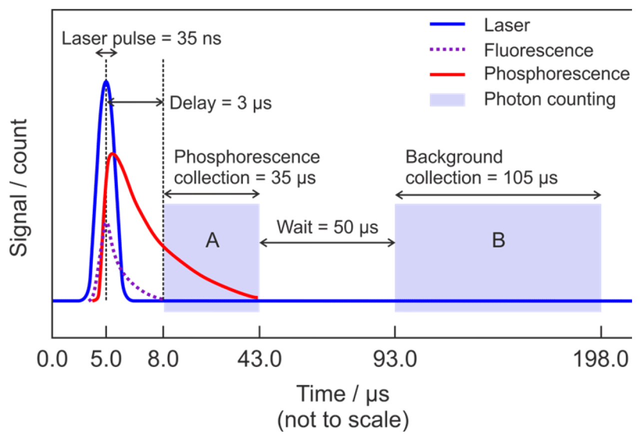
Figure 2Schematic diagram showing the timing scheme for signal acquisition. The start of the cycle (time = 0.0 µs) is defined by the laser trigger. Blue is the Ti:Sapphire laser pulse at λ∼440 nm; dashed purple is the short-lived fluorescence from the cell anodising dye, optics, and interfering species (e.g. NO2); red is the glyoxal phosphorescence; light (not to scale) blue shading is the photon counting. Region A indicates the gate for measurement of the combined phosphorescence signal, remaining laser-scattered light signal and background signal, while region B indicates the gate for measurement of the background signal alone.
The signal collected in gate A is the sum of glyoxal phosphorescence and background signal, which has contributions from PMT dark counts, ambient scattered light, and any laser-scattered light which has not completely decayed before photon counting begins. However, the signal collected in gate B is from the background only but excludes laser-scattered light. The PMT has a specified dark count rate of ∼200 s−1, giving a maximum dark count of ∼35 s−1 when integrated over the 5000 repetitions of Gate A (35 µs) in 1 s. The observed background signal, after subtraction of the dark counts, is on the order of 20 s−1 and is dominated by long-lived laser-scattered light.
The signal from glyoxal phosphorescence and laser-scattered light is calculated as
where SigGly is the signal from glyoxal phosphorescence plus laser-scattered light, SigA is the signal collected in gate A, SigB is the signal collected in gate B, and x=3 is the ratio of the width of gate B to the width of gate A. The 1 Hz SigGly data are then normalised by laser power. A measurement duty cycle of 300 s online and 120 s offline optimises the limit of detection without compromising the applicability of the offline measurement or the stability of the laser wavelength and alignment. To subtract the contribution from laser-scattered light, the mean normalised offline signal is subtracted from the mean normalised online signal for each duty cycle to give the glyoxal signal, SGly. Figure 3 shows a laser-induced phosphorescence excitation spectrum of glyoxal recorded with the LIP instrument in the laboratory. In ambient measurements, the concentration of glyoxal is determined by tuning the laser on and off the absorption or online wavelength of 440.141 nm. An offline wavelength of 440.035 nm results in an online : offline ratio of the absorption coefficients of more than 3, and switching between the two wavelengths is rapidly and reproducibly achieved by the laser tuning system.

Figure 3Laser-induced phosphorescence spectrum of molec. cm−3 glyoxal at a cell pressure of 100 Torr (∼13 300 Pa), showing the online and offline wavelengths used for ambient glyoxal measurements. All background signals have been removed from the data, with the signal thus representing glyoxal laser-induced phosphorescence for all wavelengths shown. Each data point was integrated over 1 s (5000 laser pulses). The wavelength increment between adjacent data points is 0.0008 nm.
2.2.2 Instrument calibration
The glyoxal signal, SGly, is related to the ambient glyoxal mixing ratio by the sensitivity or calibration factor, C.
A known mixing ratio of glyoxal is produced by the reaction of OH with acetylene and is used to determine C. A flow of synthetic air controlled by a mass flow controller (Brooks 5850S) is humidified by diverting a variable portion through an ambient temperature distilled water bubbler. The humidified flow is directed down a 30 cm long square-section aluminium flow tube (1.27 cm internal dimension) at ∼50 slm. A mercury pen-ray lamp (Oriel Instruments 6035) is fixed side-on to the flow tube, and a quartz (Suprasil) window transmits light from the lamp at λ=184.9 nm. Photolysis of the water vapour produces a known concentration of OH, which is determined by actinometric calibration of the lamp using N2O photolysis to give NO (Edwards et al., 2003). A mass flow controller (Brooks 5850S) delivers 450 sccm of dilute acetylene (BOC, custom mix of 2 % of acetylene in N2), which is injected into the flow downstream of the lamp. Complete conversion of OH occurs in the flow before it is sampled by the instrument. The glyoxal concentration is given by
where is the absorption cross section of water vapour at λ=184.9 nm ( cm2 molec.−1) (Cantrell et al., 1997), ϕOH is the quantum yield of OH at λ=184.9 nm, which is equal to unity, and Ft is the product of the lamp flux and the photolysis time, determined by actinometry. The yield of glyoxal from OH + acetylene (1.75) under the conditions of the calibration was determined by modelling the reaction in the chemical kinetics program Kintecus (Ianni, 2017), using a reaction mechanism and kinetics data from the Master Chemical Mechanism (http://mcm.york.ac.uk/home.htt, last access: 12 April 2022; Jenkin et al., 2003; Saunders et al., 2003) and Lockhart et al. (2013). The factor of 1.75, which is larger than unity, between [Gly] and [OH] in Eq. (3) is a result of the OH-initiated oxidation of acetylene in air, giving the product HC(O−O) = C(OH)H, which isomerises to form HC(OOH)−C(O)H, which subsequently decomposes to eliminate OH and forming glyoxal, with the OH going on to react further with acetylene to form additional glyoxal.
A range of glyoxal mixing ratios can be achieved during a calibration by changing the lamp flux. Data are processed as described above and are averaged over each mixing ratio. A straight line, weighted by the standard deviations of the mixing ratio of glyoxal and the LIP signal, is fitted to the averaged data, with the sensitivity or calibration factor, C, being equal to the gradient. The uncertainty in the calibration factor is calculated as the sum in quadrature of the standard error of the gradient and the combined uncertainty in glyoxal yield, [H2O], , Ft, online laser wavelength and laser power. Figure 4 shows a typical calibration obtained during the ORC3 campaign, with the calibration factor ranging between and count s−1 mW−1 pptv−1 during the ORC3 fieldwork.
2.2.3 Limit of detection
The minimum detectable glyoxal mixing ratio of the instrument is governed by the signal-to-noise ratio (SNR) and also by the sensitivity and the background signal. For the case of Poisson statistics, this minimum concentration is given by
where C is the sensitivity or calibration factor, P is the online laser power, σoffline is the standard deviation of the unnormalised offline signal (typically ∼6 count s−1), m is the number of 1 s online data points, and n is the number of 1 s offline data points
Since the instrument was deployed in the field for the first time during ORC3, the measurement duty cycle was initially set at 60 s online and 60 s offline () to minimise any instabilities in the background signal, the laser wavelength or alignment caused by operation of the instrument under non-laboratory conditions. The limit of detection during this phase ranged from 5.98 to 11.06 pptv. Both the online and offline measurement periods were extended later in the campaign once the stability of the instrument was characterised, to minimise the limit of detection, which then ranged from 2.55 to 9.42 pptv for an acquisition cycle of 300 s online (m=300) and 120 s (n=120) offline. For comparison with model data, the glyoxal measurements were averaged to 1 h, giving limits of detection between 0.76 and 6.94 pptv, calculated using m=2571 and n=1029 in Eq. (4).
2.2.4 Determination of the instrument zero
During ORC3 fieldwork the zero of the instrument was determined by periodically sampling synthetic air (BOC BTCA 178) and recording measurements over a number of duty cycles (each consisting of 300 s online and 120 s offline). Any difference between the mean online and offline normalised signals was then taken as the instrument zero offset. The zero was determined several times during the campaign, and the mean offset was 0.013 count s−1 mW−1, or 1.29 pptv, with a standard deviation of 0.039 count s−1 mW−1, or 3.83 pptv. Ambient concentrations were obtained by subtracting the relevant zero value from SGly before the calibration factor was applied.
2.2.5 Measurement uncertainty
The measurement uncertainty, σGly, for short averaging times is determined by the uncertainties in the calibration factor and the instrument zero, which are given by the standard error in the linear fit to the calibration data and the standard deviation of the zero measurements, respectively. The mean 1σ uncertainty for averaging times up to 7 min was 74 % during the first ORC3 measurement campaign and 59 % during the second campaign. For 1 h averaged data, the 1σ uncertainties are 27 % for the first campaign and 26 % for the second campaign.
2.3 Supporting measurements
A suite of supporting measurements were made during both campaigns, including mixing ratios of O3, CO, NOx (NO, NO2), NOy, C2 to C8 non-methane volatile organic compounds (NMVOCs), j(O1D), wavelength-dependent incoming solar radiation, wind speed and direction, air pressure and temperature, and relative humidity. Details of supporting measurements used to examine the glyoxal observations reported in this work made during ORC3 are summarised in Table 1, with time series shown in the Supplement (Figs. S1 and S2). Further details of the measurement techniques, calibration, and accuracy are given in previous work (Lee et al., 2010; Carpenter et al., 2010).
Table 1Summary of supporting measurements at the Cape Verde Atmospheric Observatory during the ORC3 campaign for periods during which glyoxal measurements were made. Zero values indicate measurements below the instrumental limit of detection. Chemical names are those used in the MCM. Details of measurement techniques, integration times, and uncertainties are given by Carpenter et al. (2010).

2.4 Deployment of the instrument at Cabo Verde
The glyoxal instrument was housed in a 40 ft long air-conditioned shipping container which has been converted into two laboratories, located on the north (windward) side of the site, approximately 55 m from the coastline. Ambient air was sampled 10 m above the ground (20 m above mean sea level) from a tower on the roof of the container into a 40 mm internal diameter glass tube (the sampling manifold), heated to 40 ∘C to minimise the loss of analytes. The flow rate through the sampling manifold, which was used to sample glyoxal, NOx, O3, CO, and VOCs, was maintained at 50 L min−1 by a KNF diaphragm vacuum pump (N 035.1.2 AT18 with an IP 44 motor) located between the two laboratories inside the container. The glyoxal inlet was connected to a glass tee piece in the sampling manifold by 5 m of in. (6.4 mm) outer diameter PFA (perfluoroalkoxy alkane) tubing (wall thickness 0.047 in. (1.2 mm); internal diameter 0.156 in. (4.0 mm)), which was heated to 40 ∘C and insulated. The residence time between the start of sampling manifold (main inlet) and the glyoxal fluorescence region was approximately 30 s. In addition to using the sampling manifold, on 2 consecutive days during the campaign, sampling was also performed for short periods through a short length of unheated tube directly out of the side of the container, with no noticeable difference observed in measured glyoxal concentrations.
The instrument was operational for 24 days and 22 nights during the first campaign (22 June to 15 July 2014), and for 25 days and 21 nights during the second campaign (18 August to 15 September 2014). Wave-breaking activity on the shore close to the measurement site produces a high concentration of sea spray aerosol. Particles that reached the detection cell of the glyoxal instrument and overlapped with the laser beam caused a sharp increase in laser-scattered light and were detected as an easily noticed large spike in the data. These spikes were removed by excluding any single 1 Hz data point that exceeded 5 times the standard deviation above the mean value over 1 duty cycle. After filtering there were 250 h (358 h in total) of online measurements from the first campaign and 227 h (318 h in total) from the second campaign.
Figure 5 shows the time series of glyoxal observations throughout both campaigns and demonstrates that glyoxal was above the LOD throughout most of the ORC3 campaign. The maximum glyoxal mixing ratio of 36.3 pptv was observed during the first campaign on 22 June 2014; however, the 24 h mean mixing ratio during campaign 1 was lower than that during campaign 2, with values of 4.9 and 6.3 pptv, respectively. Figure S3 summarises the distributions of observed glyoxal mixing ratios observed during ORC3, which also indicates that higher mixing ratios were typically observed during campaign 2. The peak in the distribution of mixing ratios during campaign 1 was (4.2±0.1) pptv, with a small difference between that of (4.3±0.1) pptv during the daytime (∼ 06:00 to ∼ 19:00) and that of (4.1±0.1) pptv during the night-time. During campaign 2, the peak in the distribution of mixing ratios was (5.2±0.1) pptv, with a more pronounced difference between daytime and night-time observations compared to campaign 1, with a value of (5.7±0.1) pptv during the daytime and (4.6±0.2) pptv during the night-time. Diurnal profiles for glyoxal are shown in Fig. 6. A weak diurnal profile is evident in the data, with the peak observed after midday and the mean daytime glyoxal mixing ratio slightly higher than the mean during the night-time (4.3 vs. 4.0 pptv for campaign 1; 5.9 vs. 5.0 pptv for campaign 2).
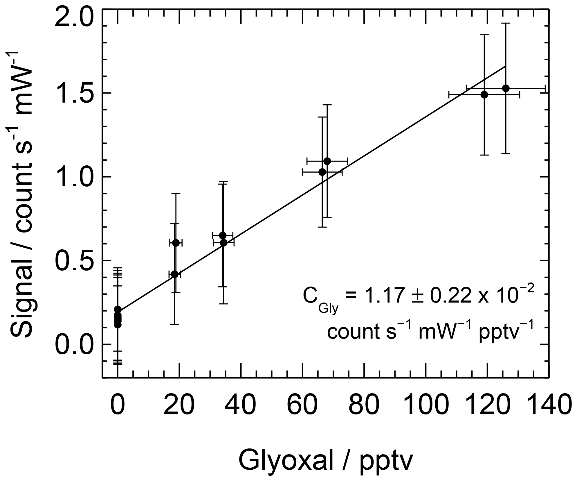
Figure 4Typical calibration plot for glyoxal obtained during ORC3, giving count s−1 mW−1 pptv−1.
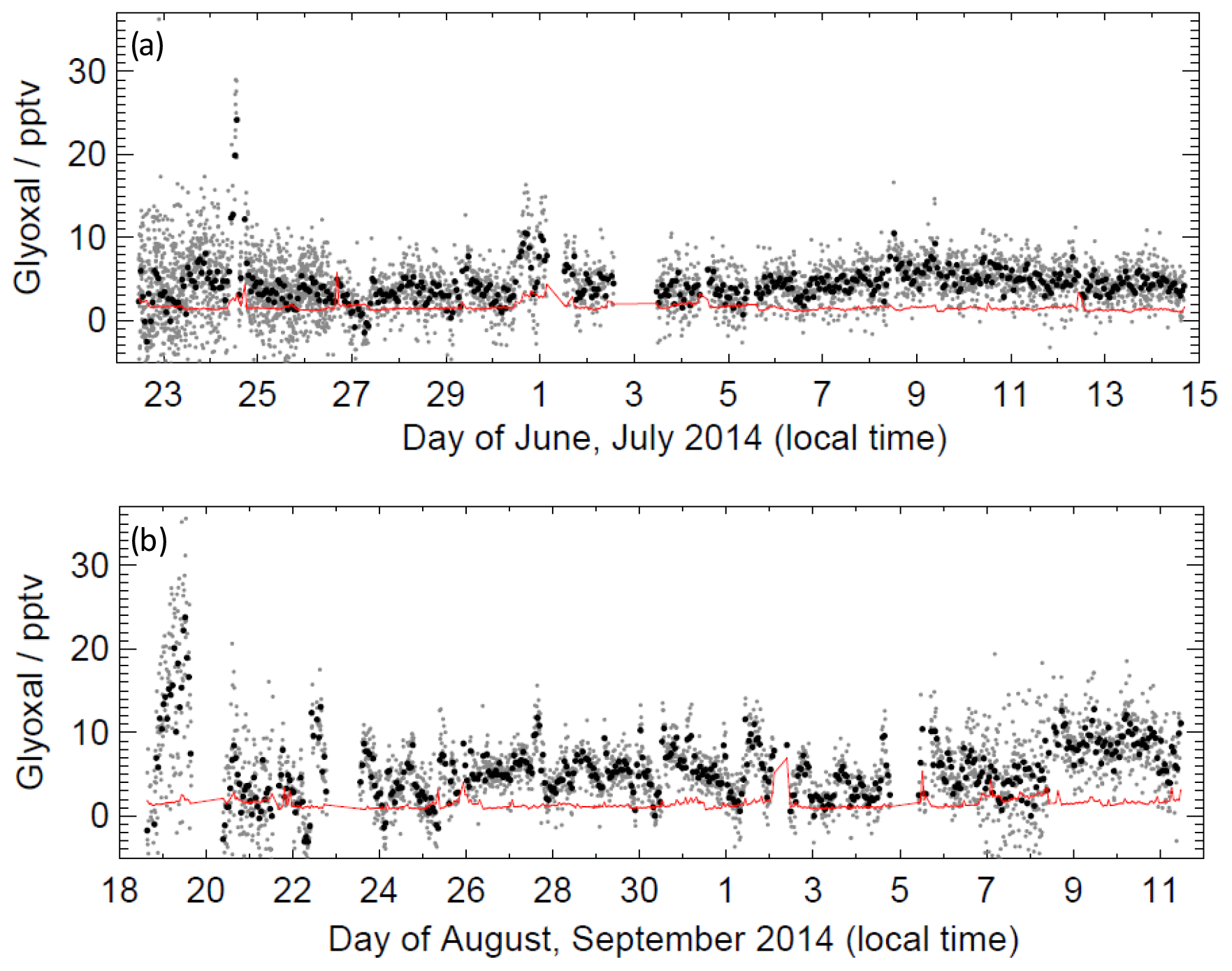
Figure 5Time series of glyoxal data during (a) campaign 1 and (b) campaign 2. Black data points show 1 h mean; grey data points show the mean for a single measurement cycle (approximately 7 min); red line shows limit of detection.
A greater variability of glyoxal with wind direction was observed during campaign 2 compared to campaign 1. A larger mean mixing ratio was observed during campaign 2, associated with air masses arriving at the CVAO site from the east and greater variability of mixing ratios in air masses arriving from the north-east (Fig. S4). Figure S5 shows the probability distribution functions for the observed glyoxal mixing ratios separated by the air mass origin as indicated by 10 d back trajectory calculations performed using the NAME dispersion model (Ryall et al., 2001) using the technique described by Carpenter et al. (2010). Most of the data correspond to air masses originating from African coastal regions or a combination of European and African coastal regions. Student's t test indicates that there is no significant difference, at the p<0.05 probability level, between data corresponding to air mass histories dominated by African coastal regions and data corresponding to the air masses dominated by a combination of European and African coastal regions. These results may imply some degree of continental influence on glyoxal abundance at CVAO. Given the short glyoxal lifetime, this influence could be via oxidation of precursors of continental origin in air masses influenced by African and/or European emission sources. A recent study examining sources and sinks of acetaldehyde in the remote Pacific atmosphere demonstrated the potential for a substantial secondary source of acetaldehyde in remote regions being missing from models (Wang et al., 2019). The potential for a similar glyoxal source in the remote atmosphere under continental outflow warrants further investigation.
Model calculations were performed using the Dynamically Simple Model of Atmospheric Chemical Complexity (DSMACC), described in detail by Emmerson and Evans (2009) and Stone et al. (2010). DSMACC represents a zero-dimensional model framework and uses the Kinetic Pre-Processor (KPP) (Sandu and Sander, 2006) with the organic chemistry scheme described by the Master Chemical Mechanism (MCM, v3.2) (http://mcm.york.ac.uk/home.htt, last access: 12 April 2022; Jenkin et al., 2003; Saunders et al., 2003) and IUPAC recommendations for kinetics of inorganic reactions (http://iupac.pole-ether.fr/, last access: 12 April 2022; Atkinson et al., 2004, 2006). The MCM describes the near-explicit oxidation schemes for 143 primary species, leading to ∼6700 species interacting in ∼17 000 reactions, and represents the most detailed and comprehensive chemistry scheme available for modelling tropospheric composition. The base model used in this work contains oxidation chemistry for methane, ethane, propane, n-butane, iso-butane, n-pentane, iso-pentane, n-hexane, ethene, propene, acetylene, isoprene, benzene, and toluene, incorporating ∼1400 species in ∼4300 reactions.
Photolysis rates in the model were calculated by the Tropospheric Ultraviolet and Visible (TUV) Radiation Model (https://www2.acom.ucar.edu/modeling/tropospheric-ultraviolet-and-visible-tuv-radiation-model, last access: 12 April 2022) and scaled to measurements of NO2 photolysis frequencies (jNO2) or to measurements of jO(1D) for O3 photolysis, made by spectral radiometry using an Ocean Optics high-resolution spectrometer (QE65000) coupled via fibre optic to a 2π quartz collection dome. The calculated photolysis frequencies for glyoxal use absorption cross sections determined by Volkamer et al. (2005) and quantum yields recommended by the NASA Panel for Data Evaluation (http://jpldataeval.jpl.nasa.gov/, last access: 12 April 2022; Sander et al., 2011).
Heterogeneous loss of HO2 and glyoxal to aerosol surfaces was represented in the model by parameterisation of a first-order loss process to the aerosol surface (Schwarz, 1986):
where k′ is the first-order rate coefficient for heterogeneous loss, r is the aerosol particle effective radius, Dg is the gas-phase diffusion coefficient (Eq. 6), γx is the uptake coefficient for species X, cg is the mean molecular speed (Eq. 7), and A is the aerosol surface area per unit volume. Dg is given by
where NA is Avogadro's number, dg is the diameter of the gas molecule, ρair is the density of air, R is the gas constant, and mg and mair are the molar masses of gas and air, respectively. cg is given by
where T is the temperature, and Mw is the molecular weight of the gas. The aerosol surface area in the model is constrained to previous measurements of dry aerosol surface area at the Cape Verde Observatory, corrected for differences in sampling height between the aerosol and glyoxal measurements and for aerosol growth under humid conditions (Allan et al., 2009; Müller et al., 2010; Whalley et al., 2010). For HO2, was used, based on the mean value reported by the parameterisation by Macintyre and Evans (2011) and consistent with values obtained in the laboratory for uptake of HO2 onto aqueous inorganic salt aerosols (George et al., 2013). For glyoxal, γCHOCHO=0.001 was used (Liggio et al., 2005; Volkamer et al., 2007; Washenfelder et al., 2011; Li et al., 2014). This value of γ for glyoxal uptake is based on studies of continental aerosol and so may not be representative of aerosol in the remote marine atmosphere. However, we find small sensitivity of simulated glyoxal in the model to the assumed value of γ. Model sensitivity to aerosol uptake for glyoxal is discussed in Sect. 5.
An additional first-order loss process for each species in the model was also included to represent deposition processes, preventing the unrealistic build-up of model-generated intermediates in the box. Deposition velocities used in the model were 0.30 cm s−1 for glyoxal (Volkamer et al., 2007; Huisman et al., 2011; Washenfelder et al., 2011; Li et al., 2014), 0.33 cm s−1 for HCHO and other aldehydes (Brasseur et al., 1998), 1.00 cm s−1 for H2O2 (Junkermann and Stockwell, 1999), and 0.90 cm s−1 for organic peroxides (ROOH) (Junkermann and Stockwell, 1999), with a fixed boundary layer height of 713 m (Carpenter et al., 2010). For all other species, the deposition rate was set to be equivalent to a lifetime of approximately 24 h. Model sensitivity to this parameter has been discussed in previous work (Stone et al., 2010, 2014), with limited sensitivity displayed by model-simulated radical species, and is discussed with reference to glyoxal in Sect. 5.
All measurements were merged onto a 1 h time base, with model calculations for glyoxal performed if observations of pressure, temperature, water vapour concentration, O3, CO, NOx, VOCs, and glyoxal were available for a specified time point, leading to a total of 872 independent simulations. For each time point, observed species are constrained to their measured value and kept constant throughout the model run. Mixing ratios of CH4 and H2 were kept constant at values of 1770 ppb (ftp://aftp.cmdl.noaa.gov/data/trace_gases/ch4/flask/surface/, last access: 12 April 2022, Dlugokencky et al., 2014) and 550 ppb (Ehhalt and Rohrer, 2009; Novelli et al., 1999), respectively, with all other species for which observations were not available set initially to zero. A summary of species used to constrain the model is given in Table 1. Nitrogen oxides (NO, NO2, NO3, N2O5, HONO, and HO2NO2) were constrained using the method described by Stone et al. (2010). Briefly, the model is initialised with the observed mixing ratio of one nitrogen oxide species, in this case NO2, and the concentrations of all nitrogen oxide species are allowed to vary according to their photochemistry as the model runs forwards. At the end of each 24 h period in the model, the calculated concentration of the nitrogen oxide species used to initialise the model is compared to its observed concentration, and the concentrations of all nitrogen oxide species fractionally increased or decreased such that the calculated concentration of the constrained species is equal to its observed concentration.
For each time point for which observations were available, the model is integrated forwards in time with diurnally varying photolysis rates until a diurnal steady state is reached, typically requiring between 5 and 10 d. Once a diurnal steady state has been reached, the concentrations of all species in the model and rates of all reactions are output for the time of day corresponding to the time at which the observations used to constrain the model were made.
5.1 Base model run
Figures 7 and 8 show the model performance for glyoxal during the two ORC3 measurement campaigns, indicating a general tendency to under-predict the glyoxal observations during both campaigns. The probability distribution functions for the modelled to observed ratios for glyoxal, separated by the air mass origin as described above for Fig. S5, are shown in Fig. S6. Student's t test indicates that there is no significant difference, at the p<0.05 probability level, between the modelled to observed ratios corresponding to air mass histories dominated by African coastal regions and data corresponding to the air masses dominated by a combination of European and African coastal regions, as also shown for the observed mixing ratios in Sect. 3. Larger average glyoxal mixing ratios observed during campaign 2 compared with campaign 1 may be linked to a shift in air mass transport patterns to Cabo Verde. During August and September (campaign 2) Cabo Verde is subject to increased influence of north-easterly and easterly air mass origins, with less influence from westerly and north-westerly remote Atlantic air masses (Carpenter et al., 2010). This shift coincides with more variable and enhanced glyoxal mixing ratios in easterly and north-easterly air masses (Fig. S5), which have had recent influence from the African coast and continent.

Figure 6The 1 h average diurnal profiles of glyoxal during (a) campaign 1 and (b) campaign 2. Error bars represent the 1σ standard deviation of the measurements. Grey shading indicates hours of darkness.
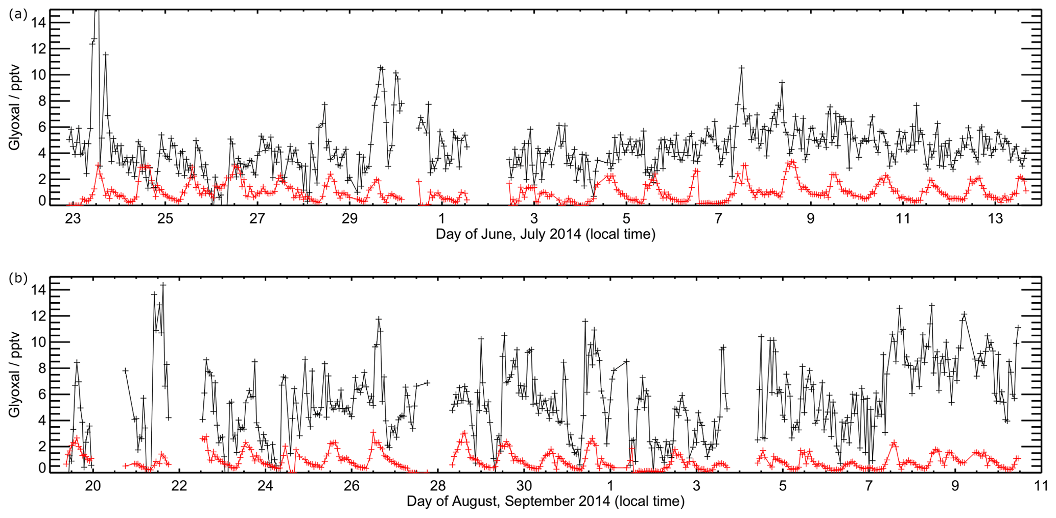
Figure 7Time series of observed (black) and modelled (red) glyoxal during ORC3. Data are shown for model output every 60 min. Panel (a) shows data from the first measurement campaign (Julian days 173 to 195), with panel (b) showing data from the second measurement campaign (Julian days 230 to 255).
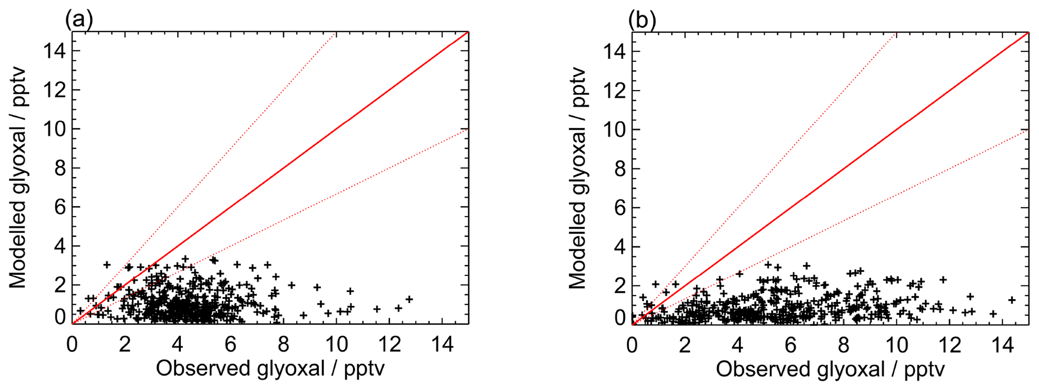
Figure 8Modelled vs observed glyoxal for (a) the first measurement period and (b) the second measurement period for the base model run. Red lines show the 1:1 line, with ±50 % given by the dashed red lines.
Figure 9 shows the average observed and modelled diurnal profiles for each measurement campaign. During the first campaign, the average observed diurnal profile ranges from 3.8 pptv at night to 5.4 pptv during the day. For the second campaign, daytime mixing ratios are typically higher, with the average observed diurnal profile ranging from a minimum of 3.4 pptv at night to a maximum of 7.7 pptv during the day. For both campaigns, the model under-predicts the observed glyoxal mixing ratios, with minima in the modelled glyoxal diurnal profiles of 0.5 and 0.3 pptv for the first and second measurement campaigns, respectively, occurring at approximately 07:00 for both campaigns, and maxima of 1.9 and 1.7 pptv around midday for campaigns 1 and 2, respectively. The modelled glyoxal mixing ratios, for both campaigns, display greater diurnal variation than is apparent in the observations, with the model under-prediction indicating either an overestimation of sinks or an underestimation of sources.

Figure 9Average observed (black) and modelled (red) glyoxal diurnal profiles for (a) the first measurement period and (b) the second measurement period for the base model run. Shaded regions show the 1σ variability of the data. Note that the diurnal profiles only include data for which supporting measurements required to run the model are available and thus show small differences from the mean diurnal profiles displayed in Fig. 6.
Diurnally averaged budget analyses for glyoxal are shown in Fig. 10, with the budgets around midday (11:00 to 13:00) shown in Fig. 11. The general trends in the budgets are similar between the two campaigns, and the following discussion focuses on the average behaviour for the two campaigns combined. The dominant sources of glyoxal in the model during the day are the reactions of OH with glycolaldehyde (2-hydroxyacetaldehyde, HOCH2CHO) and acetylene (C2H2). Glycolaldehyde is produced primarily in the model following the oxidation of ethene (C2H4), and the reaction between glycolaldehyde and OH represents, on average, 39 % of the total glyoxal production around midday, while the reaction of acetylene with OH represents, on average, 35 % of the total glyoxal production around midday. There is also significant production of glyoxal from the reaction of OH with the peroxide species HCOCH2OOH, generated following a minor channel (5 %) in the OH-initiated oxidation of acetaldehyde in reactions R1–R4, which represents 11 %, on average, of the total glyoxal production around midday.
While observations of C2H2 and C2H4 are available during the campaigns and provide a constraint on the two dominant model pathways for glyoxal production, there is no such observational constraint available for the acetaldehyde mixing ratio and its subsequent impact on glyoxal production. Results presented thus far only include acetaldehyde generated in the model following the oxidation of measured VOCs. For the first campaign, the mean model-simulated acetaldehyde mixing ratio was (14.2±6.5) pptv (median 15.0 pptv), while that for the second campaign was (15.0±5.6) pptv (median 16.3 pptv). Previous observations of acetaldehyde reported at the measurement site (Carpenter et al., 2010; Read et al., 2012) have indicated mixing ratios on the order of several hundred part per trillion by volume (pptv), while more recent airborne measurements made in the region of Cabo Verde during the ATom campaign (Apel et al., 2019; Wang et al., 2019) suggest lower mixing ratios of ∼ 200–300 pptv in between the surface and 200 m altitude in August. The impact of acetaldehyde on the model is discussed further in Sect. 5.2.
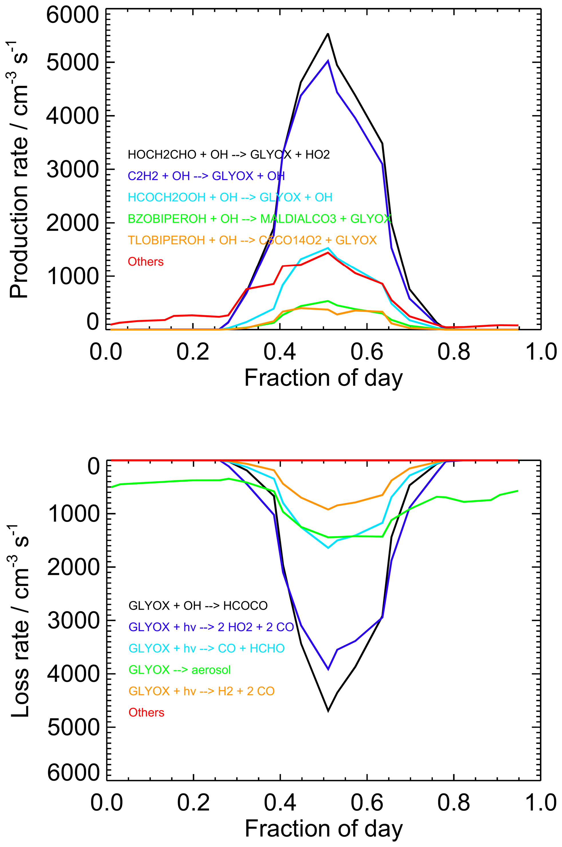
Figure 10Diurnally averaged glyoxal budgets for the base model run for both measurement periods combined. Chemical names are as given by the MCM. For information on molecular formulae and details of production mechanisms of BZOBIPEROH and TLOBIPEROH, please see http://mcm.york.ac.uk/roots.htt#aromatics (last access: 12 April 2022).

Figure 11Midday (11:00–13:00) average glyoxal budgets for the base model run for both measurement periods combined. Chemical names are as given by the MCM. Note that there are three photolysis channels contributing to the loss of glyoxal which are shown separately but constitute the dominant loss process overall. For information on molecular formulae and details of production mechanisms of BZOBIPEROH and TLOBIPEROH, please see http://mcm.york.ac.uk/roots.htt#aromatics (last access: 12 April 2022).
Several reactions comprise the remaining source term for glyoxal, notably including those involving oxidation products of benzene and toluene (for example, the MCM species BZOBIPEROH and TLOBIPEROH shown in Figs. 10 and 11), with each providing a small contribution to the total. At night, the dominant sources of glyoxal are reactions of intermediates generated by O3- or NO3-initiated oxidation of isoprene (>80 % of the total) and NO3-initiated oxidation of toluene.
Loss of glyoxal in the model is dominated by photolysis, which represents 50 % of the total sink term around midday (note that the three possible photolysis channels in the model are shown individually in Figs. 10 and 11), followed by reaction with OH (37 % of the midday sink) and uptake to aerosol (12 %). Night-time losses are dominated by uptake to aerosol and reaction with NO3. The increase in the observed-to-modelled ratio for glyoxal at night may therefore result from uncertainties in the diurnal behaviour of the aerosol surface area, with the uptake of glyoxal to aerosols potentially overestimated at night.
Modelled concentrations of OH and HO2 are similar to observations and model calculations reported previously at the Cape Verde Atmospheric Observatory (Whalley et al., 2010; Vaughan et al., 2012), with diurnal maxima of cm−3 for OH and cm−3 for HO2. Since OH is involved in both the production and loss of glyoxal, the modelled glyoxal is relatively insensitive to the concentrations of OH and HO2 in the model. Thus, while previous measurement campaigns in Cabo Verde (Read et al., 2008; Whalley et al., 2010; Stone et al., 2018) have demonstrated the importance of halogen chemistry for understanding observations of O3, OH, and HO2, the model output for glyoxal is not sensitive to halogen chemistry, and model simulations presented here do not include halogens.
5.2 Impact of acetaldehyde
The OH-initiated oxidation of acetaldehyde leads to the production of glyoxal following H-atom abstraction from the methyl group of acetaldehyde (R1–R4), which is a minor channel in the reaction between OH and acetaldehyde, with a recommended branching ratio of 0.05 (Atkinson et al., 2004). The dominant reaction channel in OH + CH3CHO, with a branching ratio of 0.95, leads to the production of acetylperoxy radicals (CH3C(O)O2) and does not result in production of glyoxal. However, the minor channel has a potentially significant impact on glyoxal, and for the base model run, unconstrained to acetaldehyde and thus using acetaldehyde concentrations generated in the model through oxidation of other measured VOCs, the minor channel in OH + CH3CHO contributes 11 % of the total glyoxal production around midday (Sect. 5.1). The production of glyoxal following the OH-initiated oxidation of acetaldehyde is thus sensitive to both concentration of acetaldehyde and the branching ratio for OH + CH3CHO.
The branching ratio for OH + CH3CHO adopted in the MCM uses the current IUPAC recommendation (Atkinson et al., 2004), which is based on experimental studies at room temperature by Cameron et al. (2002) and Butkovskaya et al. (2004). Cameron et al. (2002) used pulsed laser photolysis with direct detection of CH3CO, CH3 and H-atom products at a total pressure of 60 Torr (∼8000 Pa) to determine the branching ratios for channels producing CH3CO + H2O, CH2CHO + H2O, CH3 + HC(O)OH, and H + CH3C(O)OH and concluded that neither H nor CH3 is produced directly in the reaction between OH and acetaldehyde at detectable concentrations, with production of CH3CO (resulting from H-atom abstraction from the aldehyde group) at a yield of (0.93±0.18) and an upper limit of 0.25 for production of CH2CHO (resulting from H-atom abstraction from the methyl group). Butkovskaya et al. (2004) used a high-pressure (200 Torr, ∼26 700 Pa) turbulent flow reactor with chemical ionisation mass spectrometry, which enabled direct detection of the CH2CHO radical, giving a branching ratio for CH2CHO production of () with a total H2O yield of (0.977±0.0447), and evidence for production of glyoxal from CH2CHO in the presence of O2. The relative uncertainty in the branching ratio for H-atom abstraction from the methyl group of acetaldehyde is thus significant and has yet to be investigated over a range of temperatures and pressures.
The base model run (Sect. 5.1) was unconstrained to acetaldehyde and only contains the acetaldehyde generated in the model following the oxidation of measured VOCs, with typical acetaldehyde mixing ratios of ∼ 10–20 pptv and mean values of (14.2±6.5) pptv and (15.0±5.6) pptv for the first and second campaigns, respectively. For the base model run, over 90 % of the modelled acetaldehyde was generated following the oxidation of ethane and propene, and the model neglects potential production of acetaldehyde from oxidation of higher alkanes, as well as ocean sources of acetaldehyde, which have been shown to be significant (Singh et al., 2003; Lewis et al., 2005; Heald et al., 2008; Millet et al., 2010; Carpenter et al., 2012; Read et al., 2012; Yang et al., 2014). Measurements of higher > C5 alkanes are not available and are found to be frequently below detection limits at the CVAO site. Recent airborne measurements made near Cabo Verde during the ATom campaign have indicated acetaldehyde mixing ratios of ∼ 200–300 pptv during August 2016, measured between the ocean surface and ∼200 m altitude (Apel et al., 2019; Wang et al., 2019). The impact of acetaldehyde on glyoxal is thus likely to be underestimated by the base model run. Here, we investigate the model sensitivity to the mixing ratio of acetaldehyde using the recommended branching ratio of 0.05 (Atkinson et al., 2004) for CH3CHO + OH → CH2CHO + H2O (R1), but note that the modelled glyoxal is also sensitive to the branching ratio and that, in terms of glyoxal production, a reduction of the branching ratio to 0.04 is equivalent to a 20 % reduction in the acetaldehyde mixing ratio.
Figure 12 shows the sensitivity of glyoxal to the acetaldehyde mixing ratio in the model and compares the model output for glyoxal for the base model run (unconstrained to acetaldehyde) to a series of model runs in which acetaldehyde was constrained to a fixed mixing ratio between 25 and 500 pptv throughout each model run. There is a substantial impact on the modelled glyoxal during the day, with the modelled glyoxal approaching the observed mixing ratios during the day in the first campaign on constraint to 200 pptv acetaldehyde, which is consistent with the acetaldehyde observations made during the ATom campaign (Apel et al., 2019; Wang et al., 2019). For the model constrained to 200 pptv acetaldehyde, the production of glyoxal following OH + CH3CHO represents 56 % of the total glyoxal production at midday, with this mechanism dominating the glyoxal production for acetaldehyde mixing ratios above 100 pptv. While significantly higher mixing ratios of acetaldehyde are required to reproduce the observed glyoxal at night and during the day in the second campaign, the model results imply that the acetaldehyde mixing ratio and branching ratio for OH + CH3CHO are critical to accurately simulate glyoxal in the tropical marine environment.
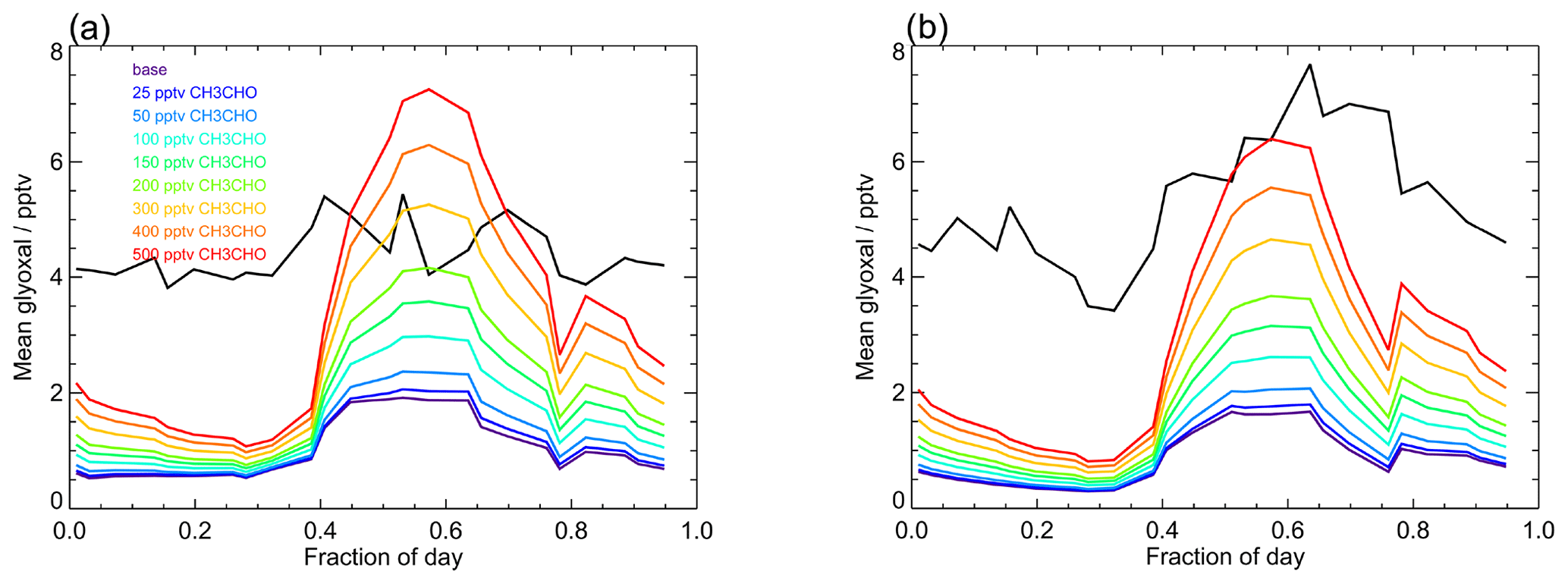
Figure 12Average observed (black) and modelled glyoxal diurnal profiles showing the sensitivity of the model to mixing ratios of acetaldehyde. The base model run includes only acetaldehyde produced within the model by the oxidation of VOCs constrained in the model (Table 1) and has mean acetaldehyde mixing ratios of (14.2±6.5) pptv during campaign 1 (median 15.0 pptv) and (15.0±5.6) pptv during campaign 2 (median 16.3 pptv). For model runs performed to investigate the sensitivity of the model to acetaldehyde, the acetaldehyde mixing ratio in each simulation was fixed to a constant mixing ratio between 25 and 500 pptv, as indicated in the legend.
5.3 Impact of terpenes
Measurements at the Cape Verde Atmospheric Observatory indicate a total of approximately 1 pptv of monoterpenes, comprising α-pinene, β-pinene, limonene, myrcene, Δ-3-carene, and ocimene (Hackenberg, 2015). Total monoterpene average mixing ratios of between 0.05 and 5 pptv have been observed in the Atlantic marine boundary layer (Hackenberg et al., 2017b) and larger average mixing ratios of 17 pptv in the North Atlantic (Kim et al., 2017). Oxidation of monoterpenes has the potential to reconcile the discrepancies between the observed and modelled glyoxal and warrants further investigation.
5.3.1 Local terpene sources
The observed monoterpene mixing ratios likely result from local sources, owing to the high reactivity of monoterpenes and their rapid photochemical removal from the atmosphere. The MCM contains full oxidation schemes for the monoterpenes α-pinene, β-pinene, and limonene (Saunders et al., 2003) and for the sesquiterpene β-caryophyllene (Jenkin et al., 2012). Impacts of these compounds on the modelled glyoxal mixing ratios were investigated by constraining the model to a range of fixed mixing ratios of each terpene, for model runs unconstrained to acetaldehyde.
The model sensitivity to the monoterpene species α-pinene and β-pinene is shown in Fig. S7. While there are some increases in the modelled glyoxal mixing ratios during the day, there are limited impacts at night, and even during the day mixing ratios of α-pinene in excess of 10 pptv (i.e. significantly in excess of observed abundance, Hackenberg, 2015) are required to reproduce the glyoxal observations. Yields of glyoxal from β-pinene, and limonene (not shown), are lower than those from α-pinene, with almost no change in the modelled glyoxal mixing ratio on inclusion of 10 pptv limonene in the model.
Glyoxal yields from the sesquiterpene β-caryophyllene, however, are higher than those for the monoterpenes. Figure S8 shows the model sensitivity to β-caryophyllene, indicating that low mixing ratios of β-caryophyllene in the model can significantly enhance the modelled glyoxal during the day. The inclusion of ∼1 and ∼2.5 pptv β-caryophyllene for the first and second campaigns, respectively, can reproduce the daytime observations of glyoxal. There is also significant production of glyoxal at night resulting from β-caryophyllene chemistry, in contrast to the monoterpenes, although higher β-caryophyllene mixing ratios (∼5 pptv in the early evening and ∼10 pptv in the early hours of the morning) are required to reproduce the night-time glyoxal observations. While such variation in the mixing ratio of a species with temperature-dependent emissions from a biogenic source is not inconceivable, particularly if the principal removal mechanism is reaction with OH, the potential role for marine sources of sesquiterpenes in the chemistry at Cabo Verde is uncertain.
Thus, while monoterpenes have the potential to produce glyoxal, the impacts are limited, and monoterpene mixing ratios higher than those observed in the Atlantic Ocean are required to explain the discrepancies between the modelled and observed glyoxal at night. In addition, given the short lifetimes of monoterpene species, significant local emissions would be required to sustain such high mixing ratios. Lower mixing ratios of the sesquiterpene β-caryophyllene are able to reproduce the glyoxal observations at night, but local sources are unknown. There is only limited indirect evidence that may support the presence of sesquiterpenes in the marine boundary layer, including measurements of markers for β-caryophyllene products in organic aerosol samples from the summertime Arctic marine atmosphere (Fu et al., 2013). However, to the best of our knowledge, there have been no direct observations of sesquiterpenes in the marine boundary layer atmosphere.
5.3.2 Remote monoterpene sources
Production of glyoxal from monoterpenes and the sesquiterpene β-caryophyllene involves a number of intermediates in multiple reactions (production following OH +α-pinene requires at least 19 reactions). Phytoplankton blooms in the South Atlantic Ocean have been shown to result in high monoterpene emissions and can lead to atmospheric mixing ratios of ∼200 pptv (Yassaa et al., 2008). Similarly, observations from the North Atlantic marine boundary layer have shown monoterpene mixing ratios as large as 100 pptv (Kim et al., 2017). There is thus potential for production of high mixing ratios of glyoxal in air masses transported from regions with high monoterpene emissions, which contain significant mixing ratios of terpene oxidation intermediates but, by the time the air mass has been transported away from the emission source, low mixing ratios of the parent monoterpene.
In order to investigate the potential for such a scenario to explain enhanced glyoxal abundances at CVAO, the model was constrained to the average mixing ratios of species observed between 10:00 and 14:00 at the Cabo Verde measurement site (Table 2) and initialised with, but not constrained to, a high monoterpene mixing ratio (100 pptv α-pinene and 50 pptv β-pinene) characteristic of a region associated with a phytoplankton bloom (Yassaa et al., 2008). The model was initialised at midday and then run forwards in time for several days to represent the chemical evolution of an air mass passing over an area with high monoterpene emissions, such as a phytoplankton bloom.
Table 2Conditions used to constrain the model run to demonstrate the downwind impact on glyoxal of remote monoterpene sources. Mixing ratios are the midday mean values of all data during both ORC3 measurement campaigns.

The impact of an air mass passing over a region with high monoterpene emissions on the monoterpene and glyoxal mixing ratios for initial monoterpene mixing ratios of 100 pptv of α-pinene and 50 pptv of β-pinene (Yassaa et al., 2008) is shown in Fig. S9. The monoterpenes are rapidly consumed (in less than 4 h), but the glyoxal mixing ratios are moderately elevated compared to equivalent model runs with no monoterpene input, owing to the chemistry of the oxidation products of the parent monoterpenes. The temporal profiles for glyoxal exhibit diurnal behaviour, maximising each day, with overall maxima observed ∼30 h after initialisation of the model, with subsequent days displaying lower maxima compared to the previous day.
The monoterpene oxidation products involved in the generation of glyoxal consist of a number of peroxide and aldehyde species, the modelled concentrations of which, in the absence of a constant monoterpene source, are influenced by the deposition rates applied to the model-generated oxidation intermediates. Figure S9 shows the impact of the deposition rate applied in the model to the evolution of glyoxal. The modelled mixing ratios of glyoxal are strongly influenced by the deposition rates applied in the model, with slower deposition rates leading to longer lifetimes of the oxidation intermediates and thus higher mixing ratios of glyoxal. In the absence of any initial monoterpene input, the modelled glyoxal mixing ratio is ∼ 2.2–2.4 pptv after ∼30 h and displays little sensitivity to the deposition rates in the model. For the model initialised with 100 pptv of α-pinene and 50 pptv of β-pinene, the modelled glyoxal varies between 2.7 pptv (using the standard deposition rates used in the model) and 3.6 pptv (with deposition rates decreased by a factor of 4).
Thus, while air masses originating from areas with high monoterpene emissions have the potential to produce elevated glyoxal mixing ratios downwind of the region with high monoterpene mixing ratios, owing to the action of the monoterpene oxidation products, the impacts are highly dependent on the deposition lifetimes applied to the model-generated intermediates. The deposition rates of such species are highly uncertain but can have significant impact on the modelled glyoxal.
5.4 Impact of physical processes
The model contains a first-order loss process for all unconstrained species to represent deposition and physical losses to prevent the build-up of unrealistic abundances of model-generated intermediates, which, for most species, is set to give a lifetime of ∼24 h. Given the significance of model-generated intermediates for the production of glyoxal, there is the potential for modelled glyoxal concentrations to be affected by the deposition rates implemented in the model. Figure S10 shows the model sensitivity to the deposition rates, and uptake of glyoxal to aerosol.
Increased deposition rates lead to a reduction in the modelled glyoxal mixing ratio, as the concentrations of intermediates such as glycolaldehyde and the peroxide HCOCH2OOH produced following the oxidation of acetaldehyde are impacted by the change in deposition rates. However, the deposition rates applied in the model would need to be reduced significantly (by more than a factor of 4) to reconcile the modelled glyoxal with the observations. A reduction in the aerosol uptake of glyoxal does improve the agreement between the modelled and observed glyoxal, particularly at night and in the early morning, potentially indicating that the constant aerosol surface area implemented in the model is uncertain and an over-simplistic approximation. However, while there is uncertainty associated with the aerosol surface area implemented in the model, the sensitivity of the modelled glyoxal to changes in the rate of aerosol uptake is not sufficient to reconcile the model with the observations.
We have made the first in situ measurements of glyoxal in the tropical remote marine boundary layer using a sensitive laser-induced phosphorescence (LIP) technique, with a temporal resolution of a few minutes. Previous remote marine glyoxal observations have mainly been based on remotely sensed measurements or coarse temporal averages using offline methods. LIP glyoxal measurements were made continuously over two 4-week campaigns during June–July and August–September 2014 at the Cape Verde Atmospheric Observatory in the tropical North Atlantic. The sensitive LIP technique achieved a limit of detection of ∼1 pptv, allowing for the measurement of 24 h average glyoxal mixing ratios of 4.9 and 6.3 pptv during the first and second campaigns respectively. The overall maximum observed mixing ratio was 36.3 pptv, measured on 22 June 2014 during campaign 2. A weak diel variation in measured glyoxal was observed, particularly during campaign 1 (daytime median 4.3±0.1 pptv; night-time median 4.1±0.2 pptv), with slightly larger diurnal variability during campaign 2 (daytime median 5.7±0.1 pptv; night-time median 4.6±0.2 pptv). Our average glyoxal mixing ratios are consistent with offline HPLC measurements made at Cape Grim on the western Tasmania coast; Lawson et al., 2015), and our highest observed mixing ratios during August-September are similar in magnitude to HPLC measurements in the South Pacific (23±8 pptv) from the same study. Our highest observed mixing ratios are also consistent with the lowest MAX-DOAS remote sensed mixing ratios in the Northern Hemisphere tropical East Pacific (Coburn et al., 2014). However, other previously measured MAX-DOAS glyoxal mixing ratios in the tropical East Pacific (range 40–140 pptv) (Sinreich et al., 2010) are substantially larger than our observed mixing ratios in the tropical Atlantic.
We found no strong relationship between the observed glyoxal abundance and air mass origin. Back trajectory calculations show some evidence for greater variability in glyoxal abundances among air masses that have been influenced by coastal and continental Africa. During August and September, greater variability in observed glyoxal with wind direction was observed, with higher median mixing ratios of 6.0 pptv associated with winds from the east and lower mixing ratios of 4.9 and 4.5 pptv from the north and north-west, respectively. During June, median mixing ratios associated with different wind sectors differed by less than 1 pptv.
The DSMACC box model with the explicit Master Chemical Mechanism, constrained by observed trace gas mixing ratios, significantly under-predicts the observed glyoxal mixing ratios during the day and night for measurements made during June–July and August–September. An investigation of the glyoxal budget in the model around local midday shows that the daytime glyoxal source is dominated by production from reactions of OH with glycolaldehyde and acetylene. During the day, a minor channel in acetaldehyde oxidation, initiated by H abstraction from the acetaldehyde methyl group, also contributes to glyoxal production. Increasing the acetaldehyde concentration in the model, which is likely underestimated in the base model run, significantly increases model-simulated glyoxal, with the mean observed-to-modelled ratios around midday (11:00–13:00) improving from 3.2 and 4.2 for campaigns 1 and 2, respectively, for the base model run to 1.3 and 1.8 on constraint to 200 pptv acetaldehyde. This acetaldehyde mixing ratio is consistent with summertime near-surface concentrations measured from the ATom aircraft campaign in the region of Cabo Verde.
The model underestimation of the observed glyoxal at night (night-time (22:00–05:00) mean observed-to-modelled ratio of 9.7) suggests there is also a missing non-photochemical glyoxal source in the model or potentially an overestimate in model sink processes. Despite the importance of direct sea–air transfer for remote marine budgets of other oxygenated VOCs (OVOCs), such as acetone, acetaldehyde, and methanol, a similar source for glyoxal would seem unlikely due to its high solubility and potential rapid consumption in surface ocean waters (Volkamer et al., 2009; Ervens and Volkamer 2010). However, eddy covariance measurements in the Southern Hemisphere tropical Pacific have shown net positive sea–air glyoxal fluxes during night-time, which are hypothesised to result from ozone-driven glyoxal production in the sea surface microlayer that outcompetes the surface deposition flux (Coburn et al., 2014). Such a source cannot be ruled out during the ORC3 campaigns and may explain at least some of the model underestimate. Ozone-driven reactions to produce glyoxal from idealised organic films in seawater have been shown from laboratory experiments (Zhou et al., 2014). Further investigation using a coupled sea–air transfer model to investigate the potential impact of such a source is warranted.
We investigated the possible role for monoterpenes as glyoxal precursors using the DSMACC model. Observed mixing ratios of monoterpenes at CVAO are insufficient to act as an appreciable source of glyoxal, and monoterpene mixing ratios larger than those observed during the ORC3 campaign are required to explain the discrepancies between the modelled and observed glyoxal. The model suggests that low mixing ratios (1–2.5 pptv) of the sesquiterpene β-caryophyllene would produce sufficient glyoxal to match observed concentrations, but there is no direct evidence for the presence of sesquiterpenes at CVAO. Using the model to simulate the potential influence of a large monoterpene source, upwind of CVAO, showed the potential to produce elevated glyoxal mixing ratios downwind of such a source via oxidation of monoterpene oxidation products. However, the magnitude of this potential source is highly sensitive to the deposition rates of the intermediate products, which are largely unknown.
Overall, our model results imply that our understanding of glyoxal in the remote marine boundary layer may be largely controlled by our knowledge of the remote marine acetaldehyde budget and acetaldehyde oxidation chemistry, in particular the mixing ratio of acetaldehyde and the branching ratios for H-atom abstraction at different sites in acetaldehyde, which are both associated with significant uncertainties. Given considerable uncertainties in our understanding of remote acetaldehyde sources, and a widespread underestimate of acetaldehyde in the remote troposphere in models (Wang et al., 2019), these factors may limit our ability to constrain the glyoxal budget in the large-scale remote atmosphere at present. In addition, improved understanding of monoterpene sources in the marine boundary layer and the influence of upwind monoterpene emissions in air masses sampled at CVAO may help constrain other potential influences on the glyoxal budget in this region. Further analysis using 3D chemical transport modelling is needed to investigate further the potential for large-scale secondary production of glyoxal from VOC precursors in the remote marine atmosphere.
The DSMACC model code is available to download from https://github.com/barronh/DSMACC (Henderson, 2022).
Glyoxal time series data from the ORC3 campaigns are available on request from the corresponding authors. Supporting atmospheric chemistry data from the CVAO are available from the Centre for Environmental Data Analysis at http://catalogue.ceda.ac.uk/uuid/81693aad69409100b1b9a247b9ae75d5 (National Centre for Atmospheric Science, 2022).
The supplement related to this article is available online at: https://doi.org/10.5194/acp-22-5535-2022-supplement.
SRA and DEH designed and led the study. HW and TI carried out glyoxal measurements. HW analysed glyoxal measurements, with support and input from DEH, SRA, DVS, LW, TI, and DC. DS carried out the box modelling. SP, KR, and LJC provided supporting measurements at Cape Verde Atmospheric Observatory used in the modelling. SH and LJC provided monoterpene measurements. HW, DS, DEH, and SRA wrote the manuscript. All authors provided comments on the analysis and manuscript.
At least one of the (co-)authors is a member of the editorial board of Atmospheric Chemistry and Physics. The peer-review process was guided by an independent editor, and the authors also have no other competing interests to declare.
Publisher's note: Copernicus Publications remains neutral with regard to jurisdictional claims in published maps and institutional affiliations.
The authors would like to thank the Natural Environment Research Council (NERC) for funding the ORC3 project (NE/K006665/1 and NE/K004980/1). Daniel Stone would also like to thank NERC for the award of an Independent Research Fellowship (IRF) (NE/L010798/1). We would also like to thank NERC for the provision of a research studentship for Danny Cryer. The authors acknowledge Luis Mendes, Instituto Nacional de Meteorologia e Geofísica, São Vicente (INMG), Mindelo, Cabo Verde, for his technical support of the measurements.
This research has been supported by the Natural Environment Research Council (grant nos. NE/K006665/1, NE/K004980/1, and NE/L010798/1).
This paper was edited by Tanja Schuck and reviewed by two anonymous referees.
Ahlm, L., Shang, L., Day, D. A., Russell, L. M., Weber, R., Gentner, D. R., Goldstein, A. H., DiGangi, J. P., Henry, S. B., Keutsch, F. N., VandenBoer, T. C., Markovic, M. Z., Murphy, J. G., Ren, X., and Scheller, S.: Formation and growth of ultrafine particles from secondary sources in Bakersfield, California, J. Geophys. Res.-Atmos, 117, 1–13, 2012.
Allan, J. D., Topping, D. O., Good, N., Irwin, M., Flynn, M., Williams, P. I., Coe, H., Baker, A. R., Martino, M., Niedermeier, N., Wiedensohler, A., Lehmann, S., Müller, K., Herrmann, H., and McFiggans, G.: Composition and properties of atmospheric particles in the eastern Atlantic and impacts on gas phase uptake rates, Atmos. Chem. Phys., 9, 9299–9314, https://doi.org/10.5194/acp-9-9299-2009, 2009.
Anderson, L. G., Parmenter, C. S., and Poland, H. M.: Collision induced intersystem crossing. The photophysics of glyoxal vapor excited at 4358 Å, Chem. Phys., 1, 401–417, 1973.
Apel, E. C., Asher, E. C., Hills, A. J., and Hornbrook, R. S.: ATom: Volatile Organic Compounds (VOCs) from the TOGA instrument, ORNL DAAC, Oak Ridge, Tennessee, USA, https://doi.org/10.3334/ORNLDAAC/1749, 2019.
Atkinson, R., Baulch, D. L., Cox, R. A., Crowley, J. N., Hampson, R. F., Hynes, R. G., Jenkin, M. E., Rossi, M. J., and Troe, J.: Evaluated kinetic and photochemical data for atmospheric chemistry: Volume I – gas phase reactions of Ox, HOx, NOx and SOx species, Atmos. Chem. Phys., 4, 1461–1738, https://doi.org/10.5194/acp-4-1461-2004, 2004.
Atkinson, R., Baulch, D. L., Cox, R. A., Crowley, J. N., Hampson, R. F., Hynes, R. G., Jenkin, M. E., Rossi, M. J., Troe, J., and IUPAC Subcommittee: Evaluated kinetic and photochemical data for atmospheric chemistry: Volume II – gas phase reactions of organic species, Atmos. Chem. Phys., 6, 3625–4055, https://doi.org/10.5194/acp-6-3625-2006, 2006.
Bloss, W. J., Evans, M. J., Lee, J. D., Sommariva, R., Heard, D. E., and Pilling, M. J.: The oxidative capacity of the troposphere: Coupling of field measurements of OH and a global chemistry transport model, Faraday Discuss., 130, 425–436, 2005.
Brasseur, G. P., Hauglustaine, D. A., Walters, S., Rasch, P. J., Muller, J. F., Granier, C., and Tie, X. X.: MOZART, a global chemical transport model for ozone and related chemical tracers, 1. Model description, J. Geophys. Res.-Atmos., 103, 28265–28289, 1998.
Butkovskaya, N. I., Kukui, A., and Le Bras, G.: Branching Fractions for H2O Forming Channels of the Reaction of OH Radicals with Acetaldehyde, J. Phys. Chem. A, 108, 1160–1168, 2004.
Cameron, M., Sivakumaran, V., Dillon, T. J., and Crowley, J. N.: Reaction between OH and CH3CHO: Part 1. Primary product yields of CH3 (296 K), CH3CO (296 K), and H (237–296 K), Phys. Chem. Chem. Phys., 4, 3628–3638, 2002.
Cantrell, C. A., Zimmer, A., and Tyndall, G. S.: Absorption cross sections for water vapor from 183 to 193 nm, Geophys. Res. Lett., 24, 2687–2687, 1997.
Carpenter, L. J., Fleming, Z. L., Read, K. A., Lee, J. D., Moller, S. J., Hopkins, J. R., Purvis, R. M., Lewis, A. C., Müller, K., Heinold, B., Herrmann, H., Wadinga Fomba, K., van Pinxteren, D., Müller, C., Tegen, I., Widensohler, A., Müller, T., Niedermeier, N., Achterberg, E. P., Patey, M. D., Kozlova, E. A., Meimann, M., Heard, D. E., Plane, J. M. C., Mahajan, A., Oetjen, H., Ingham, T., Stone, D., Whalley, L. K., Evans, M. J., Pilling, M. J., Leigh, R. L., Monks, P. S., Karunaharan, A., Vaughan, S., Arnold, S. R., Tschritter, J., Pöhler, D., Frieß, U., Holla, R., Mendes, L. M., Lopez, H., Faria, B., Manning, and A. J., Wallace, D. W. R.: Seasonal characteristics of tropical marine boundary layer air measured at the Cape Verde Atmospheric Observatory, J. Atmos. Chem., 67, 87–140, 2010.
Carpenter, L. J., Archer, S. D., and Beale, R.: Ocean-atmosphere trace gas exchange, Chem. Soc. Rev., 41, 6473–6506, 2012.
Ceburnis, D., O'Dowd, C. D., Jennings, G. S., Facchini, M. C., Emblico, L., Desesari, S., Fuzzi, S., and Sakalys, J.: Marine aerosol chemistry gradients: Elucidating primary and secondary processes and fluxes, Geophys. Res. Lett., 35, L07804, https://doi.org/10.1029/2008GL033462, 2008.
Chiu, R., Tinel, L., Gonzalez, L., Ciuraru, R., Bernard, F., George, C., and Volkamer, R.: UV photochemistry of carboxylic acids at the air-sea boundary: A relevant source of glyoxal and other oxygenated VOC in the marine atmosphere, Geophys. Res. Lett., 44, 1079–1087, 2017.
Coburn, S., Ortega, I., Thalman, R., Blomquist, B., Fairall, C. W., and Volkamer, R.: Measurements of diurnal variations and eddy covariance (EC) fluxes of glyoxal in the tropical marine boundary layer: description of the Fast LED-CE-DOAS instrument, Atmos. Meas. Tech., 7, 3579–3595, https://doi.org/10.5194/amt-7-3579-2014, 2014.
Colomb, A., Gros, V., Alvain, S., Sarda-Esteve, R., Bonsang, B., Moulin, C., Klüpfel, T., and Williams, J.: Variation of atmospheric volatile organic compounds over the Southern Indian Ocean (30–49∘ S), Environ. Chem., 6, 70–82, 2009.
DiGangi, J. P., Henry, S. B., Kammrath, A., Boyle, E. S., Kaser, L., Schnitzhofer, R., Graus, M., Turnipseed, A., Park, J.-H., Weber, R. J., Hornbrook, R. S., Cantrell, C. A., Maudlin III, R. L., Kim, S., Nakashima, Y., Wolfe, G. M., Kajii, Y., Apel, E. C., Goldstein, A. H., Guenther, A., Karl, T., Hansel, A., and Keutsch, F. N.: Observations of glyoxal and formaldehyde as metrics for the anthropogenic impact on rural photochemistry, Atmos. Chem. Phys., 12, 9529–9543, https://doi.org/10.5194/acp-12-9529-2012, 2012.
Dlugokencky, E. J., Lang, P. M., Crotwell, A. M., Masarie, K. A., and Crotwell, M. J.: Atmospheric Methane Dry Air Mole Fractions from the NOAA ESRL Carbon Cycle Cooperative Global Air Sampling Network, 1983–2013, Version: 24 June 2014, ftp://aftp.cmdl.noaa.gov/data/trace_gases/ch4/flask/surface/ (last access: 12 April 2022), 2014.
Edwards, G. D., Cantrell, C., Stephens, S., Hill, B., Goyea, O., Shetter, R., Mauldin, R. L., Kosciuch, E., Tanner, D., and Eisele, F.: Chemical Ionization Mass Spectrometer Instrument for the Measurement of Tropospheric HO2 and RO2, Anal. Chem., 75, 5317–5327, 2003.
Ehhalt, D. H. and Rohrer, F.: The tropospheric cycle of H2: a critical review, Tellus, 61B, 500–535, 2009.
Emmerson, K. M. and Evans, M. J.: Comparison of tropospheric gas-phase chemistry schemes for use within global models, Atmos. Chem. Phys., 9, 1831–1845, https://doi.org/10.5194/acp-9-1831-2009, 2009.
Ervens, B. and Volkamer, R.: Glyoxal processing by aerosol multiphase chemistry: towards a kinetic modeling framework of secondary organic aerosol formation in aqueous particles, Atmos. Chem. Phys., 10, 8219–8244, https://doi.org/10.5194/acp-10-8219-2010, 2010.
Facchini, M. C., Rinaldi, M., Decesari, S., Carbone, C., Finessi, E., Mircea, M., Fuzzi, S., Ceburnis, D., Flanagan, R., Nilsson, E. D., de Leeuw, G., Martino, M., Woeltjen, J., and O'Dowd, C. D: Primary submicron marine aerosol dominated by insoluble organic colloids and aggregates, Geophys. Res. Lett., 35, 1–5, 2008.
Fick, J., Pommer, L., Nilsson, C., and Andersson, B.: Effect of OH radicals, relative humidity, and time on the composition of the products formed in the ozonolysis of alpha-pinene, Atmos. Environ., 37, 4087–4096, 2003.
Fischer, E. V., Jacob, D. J., Millet, D. B., Yantosca, R. M., and Mao, J.: The role of the ocean in the global atmospheric budget of acetone, Geophys. Res. Lett., 39, L01807, https://doi.org/10.1029/2011GL050086, 2012.
Fu, T.-M., Jacob, D. J., Wittrock, F., Burrows, J. P., Vrekoussis, M., and Henze, D. K.: Global budgets of atmospheric glyoxal and methylglyoxal, and implications for formation of secondary organic aerosols, J. Geophys. Res.-Atmos., 113, 1–17, 2008.
Fu, P. Q., Kawamura, K., Chen, J., Charrière, B., and Sempéré, R.: Organic molecular composition of marine aerosols over the Arctic Ocean in summer: contributions of primary emission and secondary aerosol formation, Biogeosciences, 10, 653–667, https://doi.org/10.5194/bg-10-653-2013, 2013.
Gantt, B., Johnson, M. S., Meskhidze, N., Sciare, J., Ovadnevaite, J., Ceburnis, D., and O'Dowd, C. D.: Model evaluation of marine primary organic aerosol emission schemes, Atmos. Chem. Phys., 12, 8553–8566, https://doi.org/10.5194/acp-12-8553-2012, 2012.
George, I. J., Matthews, P. S. J., Whalley, L. K., Brooks, B., Goddard, A., Baeza-Romero, M. T., and Heard, D. E.: Measurements of uptake coefficients for heterogeneous loss of HO2 onto submicron inorganic salt aerosols, Phys. Chem. Chem. Phys., 15, 12829–12845, 2013.
Hackenberg, S. C.: Quantifying isoprene and monoterpenes in the remote marine environment, PhD thesis, Chemistry, University of York, United Kingdom, https://core.ac.uk/download/pdf/42605591.pdf (last access: 25 April 2022), 2015.
Hackenberg, S. C., Andrews, S. J., Airs, R., Arnold, S. R., Bouman, H. A., Brewin, R. J. W., Chance, R. J., Cummings, D., DallOlmo, G., Lewis, A. C., Minaeian, J. K., Reifel, K. M., Small, A., Tarran, G. A., Tilstone, G. H., and Carpenter, L. J.: Potential controls of isoprene in the surface ocean, Global Biogeochem. Cy., 31, 644–662, https://doi.org/10.1002/2016GB005531, 2017a.
Hackenberg, S., Andrews, S., Airs, R., Arnold, S. R., Bouman, H., Cummings, D., Lewis, A., Minaeian, J., Reifel, K., Small, A., Tarran, G., Tilstone, G., and Carpenter, L. J.: Basin-scale observations of monoterpenes in the Arctic and Atlantic Oceans, Environ. Sci. Technol., 51, 10449–10458, https://doi.org/10.1021/acs.est.7b02240, 2017b.
Heald, C. L., Goldstein, A. H., Allan, J. D., Aiken, A. C., Apel, E., Atlas, E. L., Baker, A. K., Bates, T. S., Beyersdorf, A. J., Blake, D. R., Campos, T., Coe, H., Crounse, J. D., DeCarlo, P. F., de Gouw, J. A., Dunlea, E. J., Flocke, F. M., Fried, A., Goldan, P., Griffin, R. J., Herndon, S. C., Holloway, J. S., Holzinger, R., Jimenez, J. L., Junkermann, W., Kuster, W. C., Lewis, A. C., Meinardi, S., Millet, D. B., Onasch, T., Polidori, A., Quinn, P. K., Riemer, D. D., Roberts, J. M., Salcedo, D., Sive, B., Swanson, A. L., Talbot, R., Warneke, C., Weber, R. J., Weibring, P., Wennberg, P. O., Worsnop, D. R., Wittig, A. E., Zhang, R., Zheng, J., and Zheng, W.: Total observed organic carbon (TOOC) in the atmosphere: a synthesis of North American observations, Atmos. Chem. Phys., 8, 2007–2025, https://doi.org/10.5194/acp-8-2007-2008, 2008.
Henderson, B.: Dynamically Simple Model of Atmospheric Chemical Complexity, https://github.com/barronh/DSMACC, last access: 21 April 2022.
Henry, S. B., Kammrath, A., and Keutsch, F. N.: Quantification of gas-phase glyoxal and methylglyoxal via the Laser-Induced Phosphorescence of (methyl)GLyOxal Spectrometry (LIPGLOS) Method, Atmos. Meas. Tech., 5, 181–192, https://doi.org/10.5194/amt-5-181-2012, 2012.
Holzer, W. and Ramsay, D. A.: Laser-induced emission from glyoxal, Can. J. Phys., 48, 1759–1765, 1970.
Huisman, A. J., Hottle, J. R., Coens, K. L., DiGangi, J. P., Galloway, M. M., Kammrath, A., and Keutsch, F. N.: Laser-Induced Phosphorescence for the in Situ Detection of Glyoxal at Part per Trillion Mixing Ratios, Anal. Chem., 80, 5884–5891, 2008.
Huisman, A. J., Hottle, J. R., Galloway, M. M., DiGangi, J. P., Coens, K. L., Choi, W., Faloona, I. C., Gilman, J. B., Kuster, W. C., de Gouw, J., Bouvier-Brown, N. C., Goldstein, A. H., LaFranchi, B. W., Cohen, R. C., Wolfe, G. M., Thornton, J. A., Docherty, K. S., Farmer, D. K., Cubison, M. J., Jimenez, J. L., Mao, J., Brune, W. H., and Keutsch, F. N.: Photochemical modeling of glyoxal at a rural site: observations and analysis from BEARPEX 2007, Atmos. Chem. Phys., 11, 8883–8897, https://doi.org/10.5194/acp-11-8883-2011, 2011.
Ianni, J. C.: Kintecus, Windows Version 6.01, http://www.kintecus.com/ (last access: 12 April 2022), 2017.
Jacob, D. J., Field, B. D., Jin, E. M., Bey, I., Li, Q. B., Logan, J. A., Yantosca, R. M., and Singh, H. B.: Atmospheric budget of acetone, J. Geophys. Res.-Atmos., 107, 4100, https://doi.org/10.1029/2001JD000694, 2002.
Jenkin, M. E., Saunders, S. M., Wagner, V., and Pilling, M. J.: Protocol for the development of the Master Chemical Mechanism, MCM v3 (Part B): tropospheric degradation of aromatic volatile organic compounds, Atmos. Chem. Phys., 3, 181–193, https://doi.org/10.5194/acp-3-181-2003, 2003.
Jenkin, M. E., Wyche, K. P., Evans, C. J., Carr, T., Monks, P. S., Alfarra, M. R., Barley, M. H., McFiggans, G. B., Young, J. C., and Rickard, A. R.: Development and chamber evaluation of the MCM v3.2 degradation scheme for β-caryophyllene, Atmos. Chem. Phys., 12, 5275–5308, https://doi.org/10.5194/acp-12-5275-2012, 2012.
Junkermann, W. and Stockwell, W. R.: On the budget of photooxidants in the marine boundary layer of the tropical South Atlantic, J. Geophys. Res.-Atmos., 104, 8039–8046, 1999.
Kim, M. J., Novak, G. A., Zoerb, M. C., Yang, M., Blomquist, B. W., Huebert, B. J., Cappa, C. D., and Bertram, T. H.: Air-Sea exchange of biogenic volatile organic compounds and the impact on aerosol particle size distributions, Geophys. Res. Lett., 44, 3887–3896, https://doi.org/10.1002/2017GL072975, 2017.
Knote, C., Hodzic, A., Jimenez, J. L., Volkamer, R., Orlando, J. J., Baidar, S., Brioude, J., Fast, J., Gentner, D. R., Goldstein, A. H., Hayes, P. L., Knighton, W. B., Oetjen, H., Setyan, A., Stark, H., Thalman, R., Tyndall, G., Washenfelder, R., Waxman, E., and Zhang, Q.: Simulation of semi-explicit mechanisms of SOA formation from glyoxal in aerosol in a 3-D model, Atmos. Chem. Phys., 14, 6213–6239, https://doi.org/10.5194/acp-14-6213-2014, 2014.
Kroll, J. H., Ng, N. L., Murphy, S. M., Varutbangkul, V., Flagan, R. C., and Seinfeld, J. H.: Chamber studies of secondary organic aerosol growth by reactive uptake of simple carbonyl compounds, J. Geophys. Res.-Atmos., 110, D23207, https://doi.org/10.1029/2005JD006004, 2005.
Krüger, O. and Graßl, H.: Southern Ocean phytoplankton increases cloud albedo and reduces precipitation, Geophys. Res. Lett., 38, L08809, https://doi.org/10.1029/2011GL047116, 2011.
Lawson, S. J., Selleck, P. W., Galbally, I. E., Keywood, M. D., Harvey, M. J., Lerot, C., Helmig, D., and Ristovski, Z.: Seasonal in situ observations of glyoxal and methylglyoxal over the temperate oceans of the Southern Hemisphere, Atmos. Chem. Phys., 15, 223–240, https://doi.org/10.5194/acp-15-223-2015, 2015.
Lee, J. D., McFiggans, G., Allan, J. D., Baker, A. R., Ball, S. M., Benton, A. K., Carpenter, L. J., Commane, R., Finley, B. D., Evans, M., Fuentes, E., Furneaux, K., Goddard, A., Good, N., Hamilton, J. F., Heard, D. E., Herrmann, H., Hollingsworth, A., Hopkins, J. R., Ingham, T., Irwin, M., Jones, C. E., Jones, R. L., Keene, W. C., Lawler, M. J., Lehmann, S., Lewis, A. C., Long, M. S., Mahajan, A., Methven, J., Moller, S. J., Müller, K., Müller, T., Niedermeier, N., O'Doherty, S., Oetjen, H., Plane, J. M. C., Pszenny, A. A. P., Read, K. A., Saiz-Lopez, A., Saltzman, E. S., Sander, R., von Glasow, R., Whalley, L., Wiedensohler, A., and Young, D.: Reactive Halogens in the Marine Boundary Layer (RHaMBLe): the tropical North Atlantic experiments, Atmos. Chem. Phys., 10, 1031–1055, https://doi.org/10.5194/acp-10-1031-2010, 2010.
Lerot, C., Stavrakou, T., De Smedt, I., Müller, J.-F., and Van Roozendael, M.: Glyoxal vertical columns from GOME-2 backscattered light measurements and comparisons with a global model, Atmos. Chem. Phys., 10, 12059–12072, https://doi.org/10.5194/acp-10-12059-2010, 2010.
Lerot, C., Hendrick, F., Van Roozendael, M., Alvarado, L. M. A., Richter, A., De Smedt, I., Theys, N., Vlietinck, J., Yu, H., Van Gent, J., Stavrakou, T., Müller, J.-F., Valks, P., Loyola, D., Irie, H., Kumar, V., Wagner, T., Schreier, S. F., Sinha, V., Wang, T., Wang, P., and Retscher, C.: Glyoxal tropospheric column retrievals from TROPOMI – multi-satellite intercomparison and ground-based validation, Atmos. Meas. Tech., 14, 7775–7807, https://doi.org/10.5194/amt-14-7775-2021, 2021.
Lewis, A. C., Carpenter, L. J., and Pilling, M. J.: Nonmethane hydrocarbons in Southern Ocean boundary layer air, J. Geophys. Res.-Atmos., 106, 4987–4994, 2001.
Lewis, A. C., Hopkins, J. R., Carpenter, L. J., Stanton, J., Read, K. A., and Pilling, M. J.: Sources and sinks of acetone, methanol, and acetaldehyde in North Atlantic marine air, Atmos. Chem. Phys., 5, 1963–1974, https://doi.org/10.5194/acp-5-1963-2005, 2005.
Li, X., Rohrer, F., Brauers, T., Hofzumahaus, A., Lu, K., Shao, M., Zhang, Y. H., and Wahner, A.: Modeling of HCHO and CHOCHO at a semi-rural site in southern China during the PRIDE-PRD2006 campaign, Atmos. Chem. Phys., 14, 12291–12305, https://doi.org/10.5194/acp-14-12291-2014, 2014.
Liggio, J., Li, S.-M., and McLaren, R.: Reactive uptake of glyoxal by particulate matter, J. Geophys. Res.-Atmos., 110, D10304, https://doi.org/10.1029/2004JD005113, 2005.
Lockhart, J., Blitz, M., Heard, D., Seakins, P., and Shannon, R.: Kinetic study of the OH plus glyoxal reaction: Experimental evidence and quantification of direct OH recycling, J. Phys. Chem. A., 117, 11027–11037, 2013.
Loza, C. L., Chan, A. W. H., Galloway, M. M., Keutsch, F. N., Flagan, R. C., and Seinfeld, J. H.: Characterization of Vapor Wall Loss in Laboratory Chambers, Environ. Sci. Technol., 44, 5074–5078, 2010.
Luo, G. and Yu, F.: A numerical evaluation of global oceanic emissions of α-pinene and isoprene, Atmos. Chem. Phys., 10, 2007–2015, https://doi.org/10.5194/acp-10-2007-2010, 2010.
Macintyre, H. L. and Evans, M. J.: Parameterisation and impact of aerosol uptake of HO2 on a global tropospheric model, Atmos. Chem. Phys., 11, 10965–10974, https://doi.org/10.5194/acp-11-10965-2011, 2011.
Mahajan, A. S., Whalley, L. K., Kozlova, E., Oetjen, H., Mendez, L., Furneaux, K. L., Goddard, A., Heard, D. E., Plane, J. M. C., and Saiz-Lopez, A.: DOAS observations of formaldehyde and its impact on the HOx balance in the tropical Atlantic marine boundary later, J. Atmos. Chem., 66, 167–178, 2010.
Mahajan, A. S., Prados-Roman, C., Hay, T. D., Lampel, J., Pöhler, D., Großmann, K., Tschritter, J., Frieß, U., Platt, U., Johnston, P., Kreher, K., Wittrock, F., Burrows, J. P., Plane, J. M. C., and Saiz-Lopez, A.: Glyoxal observations in the global marine boundary layer, J. Geophys. Res.-Atmos., 119, 6160–6169, 2014.
Matsunaga, S., Mochida, M., Saito, T., and Kawamura, K.: In situ measurement of isoprene in the marine air and surface seawater from the western North Pacific, Atmos. Environ., 36, 6051–6057, 2002.
Meskhidze, N. and Nenes, A.: Phytoplankton and cloudiness in the Southern Ocean, Science, 314, 1419–1423, 2006.
Meskhidze, N., Xu, J., Gantt, B., Zhang, Y., Nenes, A., Ghan, S. J., Liu, X., Easter, R., and Zaveri, R.: Global distribution and climate forcing of marine organic aerosol: 1. Model improvements and evaluation, Atmos. Chem. Phys., 11, 11689–11705, https://doi.org/10.5194/acp-11-11689-2011, 2011.
Millet, D. B., Guenther, A., Siegel, D. A., Nelson, N. B., Singh, H. B., de Gouw, J. A., Warneke, C., Williams, J., Eerdekens, G., Sinha, V., Karl, T., Flocke, F., Apel, E., Riemer, D. D., Palmer, P. I., and Barkley, M.: Global atmospheric budget of acetaldehyde: 3-D model analysis and constraints from in-situ and satellite observations, Atmos. Chem. Phys., 10, 3405–3425, https://doi.org/10.5194/acp-10-3405-2010, 2010.
Müller, K., Lehmann, S., van Pinxteren, D., Gnauk, T., Niedermeier, N., Wiedensohler, A., and Herrmann, H.: Particle characterization at the Cape Verde atmospheric observatory during the 2007 RHaMBLe intensive, Atmos. Chem. Phys., 10, 2709–2721, https://doi.org/10.5194/acp-10-2709-2010, 2010.
National Centre for Atmospheric Science, Carpenter, L. J., Hopkins, J. R., Lewis, A. C., Neves, L. M., Moller, S., Pilling, M. J., Read, K. A., Young, T. D., and Lee, J. D.: Continuous Cape Verde Atmospheric Observatory Observations, NCAS British Atmospheric Data Centre, http://catalogue.ceda.ac.uk/uuid/81693aad69409100b1b9a247b9ae75d5 (last access: 21 April 2022), 2010.
Novelli, P. C., Lang, P. M., Masarie, K. A., Hurst, D. F., Myers, R., and Elkins, J. W.: Molecular hydrogen in the troposphere: Global distribution and budget, J. Geophys. Res., 104, 30427–30444, 1999.
Nunes, F. M. N., Veloso, M. C. C., Pereira, P. A. D. P., and de Andrade, J. B.: Gas-phase ozonolysis of the monoterpenoids (S)-(+)-carvone, (R)-(-)-carvone, (-)-carveol, geraniol and citral, Atmos. Environ., 39, 7715–7730, 2005.
O'Dowd, C. O., Facchini, M. C., Cavalli, F., Ceburnis, D., Mircea, M., Decesari, S., Fuzzi, S., Yoon, Y. J., and Putaud, J.-P.: Biogenically driven organic contribution to marine aerosol, Nature, 431, https://doi.org/10.1038/nature02959, 2004.
Ovadnevaite, J., O'Dowd, C., Dall'Osto, M., Ceburnis, D., Worsnop, D. R., and Berresheim, H., Detecting high contributions of primary organic matter to marine aerosol: A case study, Geophys. Res. Lett., 38, L02807, https://doi.org/10.1029/2010GL046083, 2011.
Platnick, S. and Twomey, S.: Determining the susceptibility of cloud albedo to changes in droplet concentration with the advanced very high-resolution radiometer, J. Appl. Met., 33, 334–347, 1994.
Pusede, S. E., Gentner, D. R., Wooldridge, P. J., Browne, E. C., Rollins, A. W., Min, K.-E., Russell, A. R., Thomas, J., Zhang, L., Brune, W. H., Henry, S. B., DiGangi, J. P., Keutsch, F. N., Harrold, S. A., Thornton, J. A., Beaver, M. R., St. Clair, J. M., Wennberg, P. O., Sanders, J., Ren, X., VandenBoer, T. C., Markovic, M. Z., Guha, A., Weber, R., Goldstein, A. H., and Cohen, R. C.: On the temperature dependence of organic reactivity, nitrogen oxides, ozone production, and the impact of emission controls in San Joaquin Valley, California, Atmos. Chem. Phys., 14, 3373–3395, https://doi.org/10.5194/acp-14-3373-2014, 2014.
Read, K. A., Mahajan, A. S., Carpenter, L. J., Evans, M. J., Faria, B. V. E., Heard, D. E., Hopkins, J. R., Lee, J. D., Moller, S. J., Lewis, A. C., Mendes, L., McQuaid, J. B., Oetjen, H., Saiz-Lopez, A., Pilling, M. J., and Plane, J. M. C.: Extensive halogen mediated ozone destruction over the tropical Atlantic Ocean, Nature, 453, 1232–1235, 2008.
Read, K. A., Carpenter, L. J., Arnold, S. R., Beale, R., Nightingale, P. D., Hopkins, J. R., Lewis, A. C., Lee, J. D., Mendes, L., and Pickering, S. J.: Multiannual Observations of Acetone, Methanol, and Acetaldehyde in Remote Tropical Atlantic Air: Implications for Atmospheric OVOC Budgets and Oxidative Capacity, Environ. Sci. Technol., 46, 11028–11039, 2012.
Ryall, D. B., Derwent, R. G., Manning, A. J., Simmonds, P. G., and O'Doherty, S.: Estimating source regions of European emissions of trace gases from observations at Mace Head, Atmos. Environ., 34, 2507–2523, 2001.
Sander, S. P., Abbatt, J., Barker, J. R., Burkholder, J. B., Friedl, R. R., Golden, D. M., Huie, R. E., Kolb, C. E., Kurylo, M. J., Moortgat, G. K., Orkin, V. L., and Wine, P. H.: Chemical Kinetics and Photochemical Data for Use in Atmospheric Studies, Evaluation No. 17, JPL Publication 10-6, Jet Propulsion Laboratory, Pasadena, http://jpldataeval.jpl.nasa.gov/pdf/JPL 10-6 Final 15June2011.pdf (last access: 12 April 2022), 2011.
Sandu, A. and Sander, R.: Technical note: Simulating chemical systems in Fortran90 and Matlab with the Kinetic PreProcessor KPP-2.1, Atmos. Chem. Phys., 6, 187–195, https://doi.org/10.5194/acp-6-187-2006, 2006.
Saunders, S. M., Jenkin, M. E., Derwent, R. G., and Pilling, M. J.: Protocol for the development of the Master Chemical Mechanism, MCM v3 (Part A): tropospheric degradation of non-aromatic volatile organic compounds, Atmos. Chem. Phys., 3, 161–180, https://doi.org/10.5194/acp-3-161-2003, 2003.
Schwarz, S.E.: Mass-transport considerations pertinent to aqueous phase reactions of gases in liquid-water clouds, Chemistry of Multiphase Atmospheric Systems, NATO ASI Series, G6, edited by: Jaeschke, W., Springer-Verlag, Berlin, 415–471, https://doi.org/10.1007/978-3-642-70627-1_16, 1986.
Singh, H. B., Tabazadeh, A., Evans, M. J., Field, B. D., Jacob, D. J., Sachse, G., Crawford, J. H., Shetter, R., and Brune, W. H.: Oxygenated volatile organic chemicals in the oceans: Inferences and implications based on atmospheric observations and air-sea exchange models, Geophys. Res. Lett., 30, 1–4, https://doi.org/10.1029/2003GL017933, 2003.
Sinreich, R., Volkamer, R., Filsinger, F., Frieß, U., Kern, C., Platt, U., Sebastián, O., and Wagner, T.: MAX-DOAS detection of glyoxal during ICARTT 2004, Atmos. Chem. Phys., 7, 1293–1303, https://doi.org/10.5194/acp-7-1293-2007, 2007.
Sinreich, R., Coburn, S., Dix, B., and Volkamer, R.: Ship-based detection of glyoxal over the remote tropical Pacific Ocean, Atmos. Chem. Phys., 10, 11359–11371, https://doi.org/10.5194/acp-10-11359-2010, 2010.
Spracklen, D. V., Arnold, S. R., Sciare, J., Carslaw, K. S., and Pio, C.: Globally significant oceanic source of organic carbon, Geophys. Res. Lett., 35, L12811, https://doi.org/10.1029/2008GL033359, 2008.
Stone, D., Evans, M. J., Commane, R., Ingham, T., Floquet, C. F. A., McQuaid, J. B., Brookes, D. M., Monks, P. S., Purvis, R., Hamilton, J. F., Hopkins, J., Lee, J., Lewis, A. C., Stewart, D., Murphy, J. G., Mills, G., Oram, D., Reeves, C. E., and Heard, D. E.: HOx observations over West Africa during AMMA: impact of isoprene and NOx, Atmos. Chem. Phys., 10, 9415–9429, https://doi.org/10.5194/acp-10-9415-2010, 2010.
Stone, D., Evans, M. J., Walker, H., Ingham, T., Vaughan, S., Ouyang, B., Kennedy, O. J., McLeod, M. W., Jones, R. L., Hopkins, J., Punjabi, S., Lidster, R., Hamilton, J. F., Lee, J. D., Lewis, A. C., Carpenter, L. J., Forster, G., Oram, D. E., Reeves, C. E., Bauguitte, S., Morgan, W., Coe, H., Aruffo, E., Dari-Salisburgo, C., Giammaria, F., Di Carlo, P., and Heard, D. E.: Radical chemistry at night: comparisons between observed and modelled HOx, NO3 and N2O5 during the RONOCO project, Atmos. Chem. Phys., 14, 1299–1321, https://doi.org/10.5194/acp-14-1299-2014, 2014.
Stone, D., Sherwen, T., Evans, M. J., Vaughan, S., Ingham, T., Whalley, L. K., Edwards, P. M., Read, K. A., Lee, J. D., Moller, S. J., Carpenter, L. J., Lewis, A. C., and Heard, D. E.: Impacts of bromine and iodine chemistry on tropospheric OH and HO2: comparing observations with box and global model perspectives, Atmos. Chem. Phys., 18, 3541–3561, https://doi.org/10.5194/acp-18-3541-2018, 2018.
van Pinxteren, M. and Herrmann, H.: Glyoxal and methylglyoxal in Atlantic seawater and marine aerosol particles: method development and first application during the Polarstern cruise ANT XXVII/4, Atmos. Chem. Phys., 13, 11791–11802, https://doi.org/10.5194/acp-13-11791-2013, 2013.
Vaughan, S., Ingham, T., Whalley, L. K., Stone, D., Evans, M. J., Read, K. A., Lee, J. D., Moller, S. J., Carpenter, L. J., Lewis, A. C., Fleming, Z. L., and Heard, D. E.: Seasonal observations of OH and HO2 in the remote tropical marine boundary layer, Atmos. Chem. Phys., 12, 2149–2172, https://doi.org/10.5194/acp-12-2149-2012, 2012.
Volkamer, R., Spietz, P., Burrows, J. P., and Platt, U.: High-resolution absorption cross-section of glyoxal in the UV-vis and IR spectral ranges, J. Photochem. Photobiol. A: Chem., 172, 35–36, 2005.
Volkamer, R., San Martini, F., Molina, L. T., Salcedo, D., Jimenez, J. L., and Molina, M. J.: A missing sink for gas-phase glyoxal in Mexico City: Formation of secondary organic aerosol, Geophys. Res. Lett., 34, L19807, https://doi.org/10.1029/2007gl030752, 2007.
Volkamer, R., Ziemann, P. J., and Molina, M. J.: Secondary Organic Aerosol Formation from Acetylene (C2H2): seed effect on SOA yields due to organic photochemistry in the aerosol aqueous phase, Atmos. Chem. Phys., 9, 1907–1928, https://doi.org/10.5194/acp-9-1907-2009, 2009.
Volkamer, R., Baidar, S., Campos, T. L., Coburn, S., DiGangi, J. P., Dix, B., Eloranta, E. W., Koenig, T. K., Morley, B., Ortega, I., Pierce, B. R., Reeves, M., Sinreich, R., Wang, S., Zondlo, M. A., and Romashkin, P. A.: Aircraft measurements of BrO, IO, glyoxal, NO2, H2O, O2–O2 and aerosol extinction profiles in the tropics: comparison with aircraft-/ship-based in situ and lidar measurements, Atmos. Meas. Tech., 8, 2121–2148, https://doi.org/10.5194/amt-8-2121-2015, 2015.
Vrekoussis, M., Wittrock, F., Richter, A., and Burrows, J. P.: Temporal and spatial variability of glyoxal as observed from space, Atmos. Chem. Phys., 9, 4485–4504, https://doi.org/10.5194/acp-9-4485-2009, 2009.
Wang, L., Khalizov, A. F., Zheng, J., Xu, W., Ma, Y., Lal, V., and Zhang, R. Y.: Atmospheric nanoparticles formed from heterogeneous reactions of organics, Nat. Geo., 3, 238–242, 2010.
Wang, S. Y., Hornbrook, R. S., Hills, A., Emmons, L. K., Tilmes, S., Lamarque, J. F., Jimenez, J. L., Campuzano-Jost, P., Nault, E. A., Crounse, J. D., Wennberg, P. O., Kim, M., Allen, H. Ryerson, T. B., Thompson, C. R., Peischl, J., Moore, F., Nance, D., Hall, B., Elkins, J., Tanner, D., Huey, L. G., Hall, S. R., Ullmann, K., Orlando, J. J., Tyndall, G. S., Flocke, F. M., Ray, E., Hanisco, T. F., Wolfe, G. M., St Clair, J., Commane, R., Daube, B., Barletta, B., Blake, D. R., Weinzierl, B., Dollner, M., Conley, A., Vitt, F., Wofsy, S. C., Riemer, D. D., and Apel, E. C.: Atmospheric acetaldehyde: Importance of sea-air exchange and a missing source in the remote troposphere, Geophys. Res. Lett., 46, 5601–5613, 2019.
Wang, S. Y., Apel, E. C., Schwantes, R. H., Bates, K. H., Jacob, D. J., Fischer, E. V., Hornbrook, R. S., Hills, A. J., Emmons, L. K., Pan, L. L., Honomichl, S., Tilmes, S., Lamarque, J. F., Yang, M. X., Marandino, C. A., Saltzman, E. S., de Bruyn, W., Kameyama, S., Tanimoto, H., Omori, Y., Hall, S. R., Ullmann, K., Ryerson, T. B., Thompson, C. R., Peischl, J., Daube, B. C., Commane, R., McKain, K., Sweeney, C., Thames, A. B., Miller, D. O., Brune, W. H., Diskin, G. S., DiGangi, J. P., and Wofsy, S. C.: Global atmospheric budget of acetone: Air-sea exchange and the contribution to hydroxyl radicals, J. Geophys. Res.-Atmos., 125, 5, https://doi.org/10.1029/2020JD032553, 2020.
Washenfelder, R. A., Young, C. J., Brown, S. S., Angevine, W. M., Atlas, E. L., Blake, D. R., Bon, D. M., Cubison, M. J., de Gouw, J. A., Dusanter, S., Flynn, J., Gilman, J. B., Graus, M., Griffith, S., Grossberg, N., Hayes, P. L., Jimenez, J. L., Kuster, W. C., Lefer, B. L., Pollack, I. B., Ryerson, T. B., Stark, H., Stevens, P. S., and Trainer, M. K.: The glyoxal budget and its contribution to organic aerosol for Los Angeles, California, during CalNex 2010, J. Geophys. Res., 116, D00V02, https://doi.org/10.1029/2011JD016314, 2011.
Whalley, L. K., Furneaux, K. L., Goddard, A., Lee, J. D., Mahajan, A., Oetjen, H., Read, K. A., Kaaden, N., Carpenter, L. J., Lewis, A. C., Plane, J. M. C., Saltzman, E. S., Wiedensohler, A., and Heard, D. E.: The chemistry of OH and HO2 radicals in the boundary layer over the tropical Atlantic Ocean, Atmos. Chem. Phys., 10, 1555–1576, https://doi.org/10.5194/acp-10-1555-2010, 2010.
Wittrock, F., Richter, A., Oetjen, H., Burrows, J. P., Kanakidou, M., Myriokefalitakis, S., Volkamer, R., Beirle, S., Platt, U., and Wagner, T.: Simultaneous global observations of glyoxal and formaldehyde from space, Geophys. Res. Lett., 33, L16804, https://doi.org/10.1029/2006GL026310, 2006.
Yang, M., Beale, R., Liss, P., Johnson, M., Blomquist, B., and Nightingale, P.: Air–sea fluxes of oxygenated volatile organic compounds across the Atlantic Ocean, Atmos. Chem. Phys., 14, 7499–7517, https://doi.org/10.5194/acp-14-7499-2014, 2014.
Yassaa, N., Peeken, I., Zollner, E., Bluhm, K., Arnold, S., Spracklen, D., and Williams, J.: Evidence for marine production of monoterpenes, Environ. Chem., 5, 391–401, 2008.
Yokouchi, Y., Li, H.-J., Machida, T., Aoki, S., and Akimoto, H.: Isoprene in the marine boundary layer (southeast Asian Sea, eastern Indian Ocean, and Southern Ocean): Comparison with dimethyl sulphide and bromoform, J. Geophys. Res.-Atmos., 104, 8067–8076, 1999.
Yu, J. Z., Flagan, R. C., and Seinfeld, J. H.: Identification of products containing -COOH, -OH, and -C = O in atmospheric oxidation of hydrocarbons, Environ. Sci. Technol., 32, 2357–2370, 1998.
Zhou, X. L. and Mopper, K.: Photochemical production of low-molecular-weight carbonyl compounds in seawater and surface microlayer and their air-sea exchange, Mar. Chem., 56, 201–213, 1997.
Zhou, S., Gonzalez, L., Leithead, A., Finewax, Z., Thalman, R., Vlasenko, A., Vagle, S., Miller, L. A., Li, S.-M., Bureekul, S., Furutani, H., Uematsu, M., Volkamer, R., and Abbatt, J.: Formation of gas-phase carbonyls from heterogeneous oxidation of polyunsaturated fatty acids at the air–water interface and of the sea surface microlayer, Atmos. Chem. Phys., 14, 1371–1384, https://doi.org/10.5194/acp-14-1371-2014, 2014.
- Abstract
- Introduction
- Oceanic Reactive Carbon: Chemistry-Climate impacts (ORC3) campaigns and glyoxal observations
- Overview of glyoxal measurements during ORC3
- Model simulations
- Evaluation of model performance
- Conclusions and implications
- Code availability
- Data availability
- Author contributions
- Competing interests
- Disclaimer
- Acknowledgements
- Financial support
- Review statement
- References
- Supplement