the Creative Commons Attribution 4.0 License.
the Creative Commons Attribution 4.0 License.
 | 25 Apr 2022
Influences of an entrainment–mixing parameterization on numerical simulations of cumulus and stratocumulus clouds
Xiaoqi Xu
Chunsong Lu
Shi Luo
Satoshi Endo
Yuan Wang
Different entrainment–mixing processes can occur in clouds; however, a homogeneous mixing mechanism is often implicitly assumed in most commonly used microphysics schemes. Here, we first present a new entrainment–mixing parameterization that uses the grid mean relative humidity without requiring the relative humidity of the entrained air. Then, the parameterization is implemented in a microphysics scheme in a large eddy simulation model, and sensitivity experiments are conducted to compare the new parameterization with the default homogeneous entrainment–mixing parameterization. The results indicate that the new entrainment–mixing parameterization has a larger impact on the number concentration, volume mean radius, and cloud optical depth in the stratocumulus case than in the cumulus case. This is because inhomogeneous and homogeneous mixing mechanisms dominate in the stratocumulus and cumulus cases, respectively, which is mainly due to the larger turbulence dissipation rate in the cumulus case. Because stratocumulus clouds break up during the dissipation stage to form cumulus clouds, the effects of this new entrainment–mixing parameterization during the stratocumulus dissipation stage are between those during the stratocumulus mature stage and the cumulus case. A large aerosol concentration can enhance the effects of this new entrainment–mixing parameterization by decreasing the cloud droplet size and evaporation timescale. The results of this new entrainment–mixing parameterization with grid mean relative humidity are validated by the use of a different entrainment–mixing parameterization that uses parameterized entrained air properties. This study sheds new light on the improvement of entrainment–mixing parameterizations in models.
- Article
(1786 KB) - Full-text XML
- BibTeX
- EndNote


The process of entrainment and subsequent mixing between clouds and their environment is one of the most uncertain processes in cloud physics, which is thought to be crucial to many outstanding issues, including warm rain initiation and subsequent precipitation characteristics, cloud–climate feedback, and evaluating the indirect effects of aerosol (Paluch and Baumgardner, 1989; Yum, 1998; Ackerman et al., 2004; Kim et al., 2008; Huang et al., 2008; Del Genio and Wu, 2010; Lu et al., 2011, 2014; Kumar et al., 2013; Zheng and Rosenfeld, 2015; Fan et al., 2016; Gao et al., 2020, 2021; Zhu et al., 2021; Xu et al., 2021; Yang et al., 2016, 2021). The most well-studied concepts are homogeneous/inhomogeneous entrainment–mixing mechanisms. During homogeneous mixing, all droplets experience evaporation, and no droplet is evaporated completely. During extremely inhomogeneous mixing, some droplets near the entrained air evaporate completely, while the remaining droplets maintain their original sizes. If the situation is somewhere between these two extreme scenarios, an inhomogeneous mixing process occurs. Some studies suggest that homogeneous mixing is likely to be typical (Jensen et al., 1985; Burnet and Brenguier, 2007; Lehmann et al., 2009), whereas others have claimed that an extremely inhomogeneous scenario is dominant (Pawlowska et al., 2000; Burnet and Brenguier, 2007; Haman et al., 2007; Freud et al., 2008, 2011). Different mechanisms can be undistinguishable when the relative humidity in the entrained air is high (Gerber et al., 2008).
Some sensitivity studies assuming homogeneous or extremely inhomogeneous mixing have found that different mixing mechanisms can significantly influence the microphysics and radiative properties of clouds (Lasher-Trapp et al., 2005; Grabowski, 2006; Chosson et al., 2007; Slawinska et al., 2008). For example, Grabowski (2006) used a cloud-resolving model and found that the amount of solar energy reaching the surface in the pristine case, assuming the homogeneous mixing scenario, is the same as in the polluted case with extremely inhomogeneous mixing. This result was verified by Slawinska et al. (2008) using a large-eddy simulation (LES) model. Although the influence of different mixing mechanisms in simulations is lower when two-moment microphysics schemes are used (Hill et al., 2009; Grabowski and Morrison, 2011; Slawinska et al., 2012; Xu et al., 2020), Hill et al. (2009) also claimed that there are still many uncertainties in the entrainment–mixing process, and the effect of different mixing mechanisms can be more important over the entire cloud life-cycle.
In recent years, methods have been developed to describe general entrainment–mixing processes, with homogeneous and extremely inhomogeneous scenarios as special cases (Andrejczuk et al., 2006, 2009; Lehmann et al., 2009; Lu et al., 2011). Hoffmann et al. (2019) and Hoffmann and Feingold (2019) conducted LESs at the subgrid scale with turbulent mixing using a linear eddy model. Andrejczuk et al. (2009) used the results of direct numerical simulation (DNS) to establish a relationship between instantaneous microphysical properties and Damköhler number (Da; Burnet and Brenguier, 2007) and developed a parameterization of the entrainment–mixing process. Lu et al. (2013) developed a parameterization of the entrainment–mixing process based on the relationship between the homogeneous mixing degree (ψ) and transition scale number (NL) in the explicit mixing parcel model (EMPM), as well as aircraft observation data. Gao et al. (2018) investigated how ψ is related to Da and NL in a DNS to improve the parameterization of the entrainment–mixing process. Luo et al. (2020) simulated more than 12 000 cases with EMPM by changing a variety of parameters affecting entrainment–mixing processes and developed a parameterization that improved the one proposed by Lu et al. (2013).
Although several entrainment–mixing parametrizations have been proposed, to the best of our knowledge, only one study (Jarecka et al., 2013) has coupled an entrainment–mixing parameterization with cloud microphysics to consider the change in cloud droplet concentration during the entrainment–mixing process. Jarecka et al. (2013) applied an entrainment–mixing parameterization, in terms of the Damköhler number, to a two-moment microphysics scheme and found small impacts of entrainment–mixing parameterization in shallow cumulus clouds. To further explore the influences of entrainment–mixing processes, this study first modifies the entrainment–mixing parameterization in terms of the transition scale number proposed by Luo et al. (2020) to couple it more easily with microphysics schemes. The parameterization is then implemented in the two-moment Thompson aerosol-aware scheme (Thompson and Eidhammer, 2014). Finally, the effects of parameterization on the physical properties of clouds are examined in both cumulus and stratocumulus clouds.
The rest of this paper is organized as follows: Sect. 2 describes the new entrainment–mixing parameterization, simulated cases, and modeling setup. The major results are presented and discussed in Sect. 3. The influences of the new entrainment–mixing parameterization on cloud physics and the underlying mechanisms are examined, and the effects of turbulence dissipation rate (ε) and aerosol concentration are also discussed. Some concluding remarks are presented in Sect. 4.
2.1 The new entrainment–mixing parameterization
According to Morrison and Grabowski (2008), the effect of the entrainment–mixing process on cloud microphysical properties can be expressed as follows:
where Nc and Nc0 are the cloud droplet number concentrations after and before the evaporation process, respectively, and qc and qc0 represent the corresponding cloud water mixing ratios. It is noteworthy that when a new saturation is achieved after evaporation, qc is determined by qc0, relative humidity (RH), air pressure, and temperature. The parameter α can be pre-set to any value between 0 (homogeneous mixing) and 1 (extremely inhomogeneous mixing) to represent a different degree of subgrid-scale mixing homogeneity. In this study, instead of specifying α as a predetermined constant, here it is determined through the following expressions (Lu et al., 2013; Luo et al., 2020):
where a, b, and c are the three fitting parameters (Luo et al., 2020). The dimensionless number NL is a dynamical measure of the degree of subgrid-scale mixing homogeneity (Lu et al., 2011) defined by
where L∗ is the transition length (Lehmann et al., 2009), η is the Kolmogorov microscale, ν is the kinematic viscosity, and ε is calculated from the subgrid turbulent kinetic energy (Deardorff, 1980):
where C=0.70 is an empirical constant, E is the subgrid turbulent kinetic energy, and L is the model grid size. The evaporation timescale (τevap) is defined as the time taken for droplets to evaporate completely in an unsaturated environment and is calculated as
where r is the volume mean radius of cloud droplets, A is a function of pressure and temperature, Se is the supersaturation (RH − 1) of entrained air, Lh is the latent heat, Rv is the specific gas constant for water vapor, T is air temperature, ρL is the density of liquid water, K is the coefficient of thermal conductivity of air, D is the diffusion coefficient of water vapor in the air, and es(T) is the saturation vapor pressure over a plane water surface at temperature T.
Unfortunately, Se in Eq. (5a) is generally unavailable in atmospheric models, including LES models. Thus, the entrainment–mixing parameterization developed by Luo et al. (2020) based on the properties of entrained air cannot be used directly. To solve this problem, we modify the entrainment–mixing parameterization of Luo et al. (2020) by replacing Se with the domain mean RH in the EMPM, after entrainment but before evaporation, based on 12 218 cases:
Figure 1 shows the fitting results of the modified new entrainment–mixing parameterization. Compared to the parametrization proposed by Luo et al. (2020), the modified parameterization has similar ψ−NL distributions but with a larger NL for the same ψ because the EMPM domain mean RH is larger than the entrained air RH. With this modification, NL, ψ, and thus the effect of the entrainment–mixing processes on droplet concentration can be directly calculated using the LES grid mean RH. It is important to note that the parameterization does not mean that the entrained air RH is equal to that of the LES grid mean RH. It is also worth noting that a wide range of ε, Se, and fraction of entrained air (f) are taken into account when establishing the parameterization with the EMPM. The details of the EMPM simulations and related calculations are provided by Luo et al. (2020).
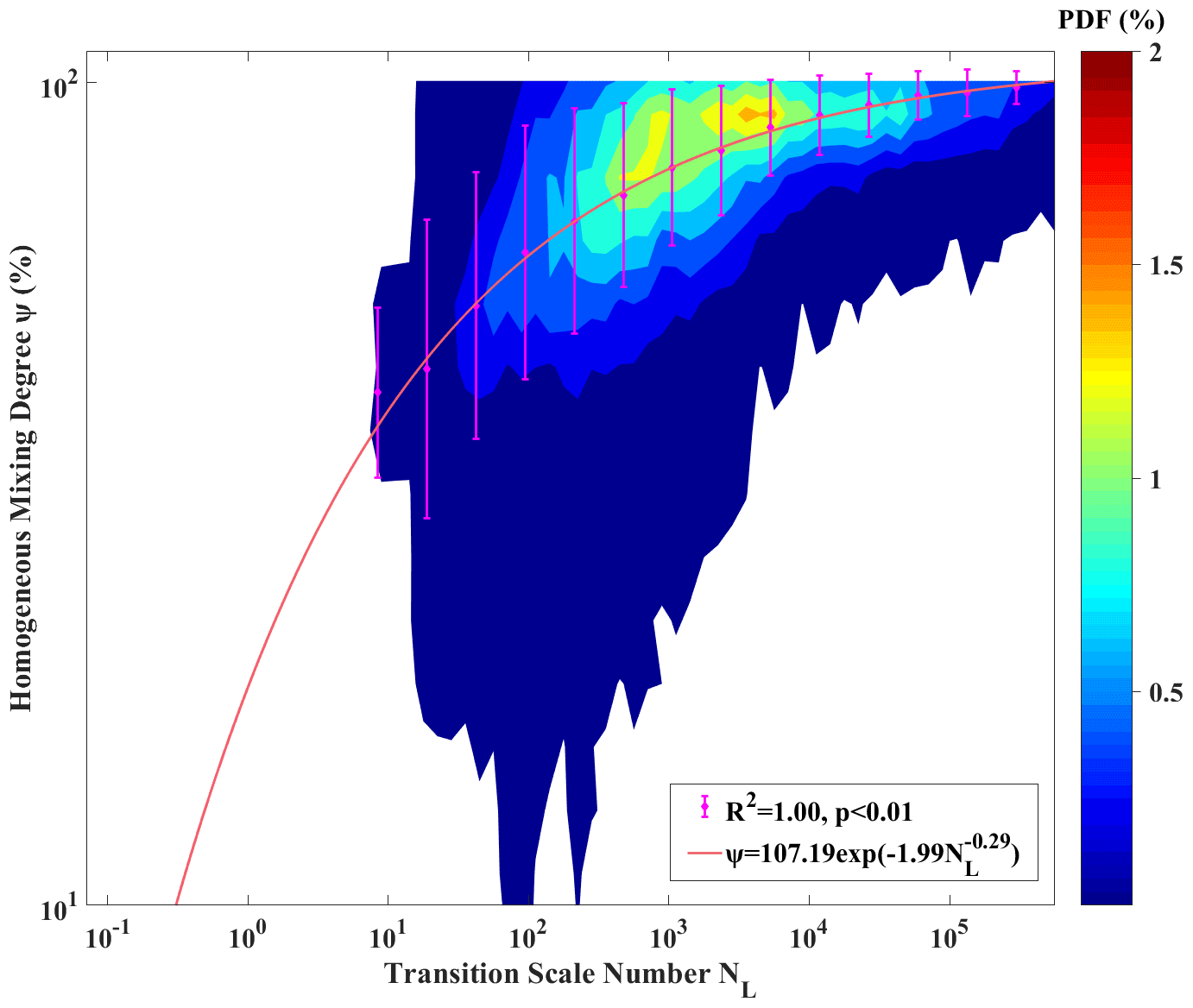
Figure 1Parameterization of cloud entrainment–mixing mechanisms by relating homogeneous mixing degree (ψ) to transition scale number (NL) from EMPM. The contours represent the joint probability distribution function (PDF) of ψ vs. NL. The magenta dots and error bars are mean values and standard deviations of ψ in each NL bin, respectively. The mean values are fitted using a weighted least squares method with the number of data points in each NL bin as with the weight. The fitting equation, coefficient of determination (R2), and p values are also given. NL is calculated with the domain-averaged relative humidity after entrainment but before evaporation in the EMPM.
2.2 LES model, simulation cases, and modeling setup
The LES model is built by applying the large-scale forcing module presented in Endo et al. (2015) to the Weather Research and Forecasting (WRF) model tailored for solar irradiance forecasting (WRF-Solar; Hacker et al., 2016; Haupt et al., 2016). The large-scale forcing data (VARANAL) used in this process are derived from the constrained variational analysis (CVA) approach developed by Zhang et al. (2001) and provided by the U.S. Department of Energy's Atmospheric Radiation Measurement Program (http://www.arm.gov, last access: 20 March 2022). The modified entrainment–mixing parameterization is implemented in the two-moment Thompson aerosol-aware scheme (Thompson and Eidhammer, 2014).
To investigate the behaviors of the new entrainment–mixing parameterization in different cloud types, cumulus and stratocumulus cases are simulated. For both the cumulus and stratocumulus cases, the horizontal resolution of the model is 100 m × 100 m with a domain area of 14.4 km × 14.4 km. The vertical direction is divided into 225 layers with a resolution of 30 m.
Table 1Summary of names and corresponding descriptions of the four experiments for each case of cumulus and stratocumulus. The meaning of each symbol for each experiment can be found in the text.
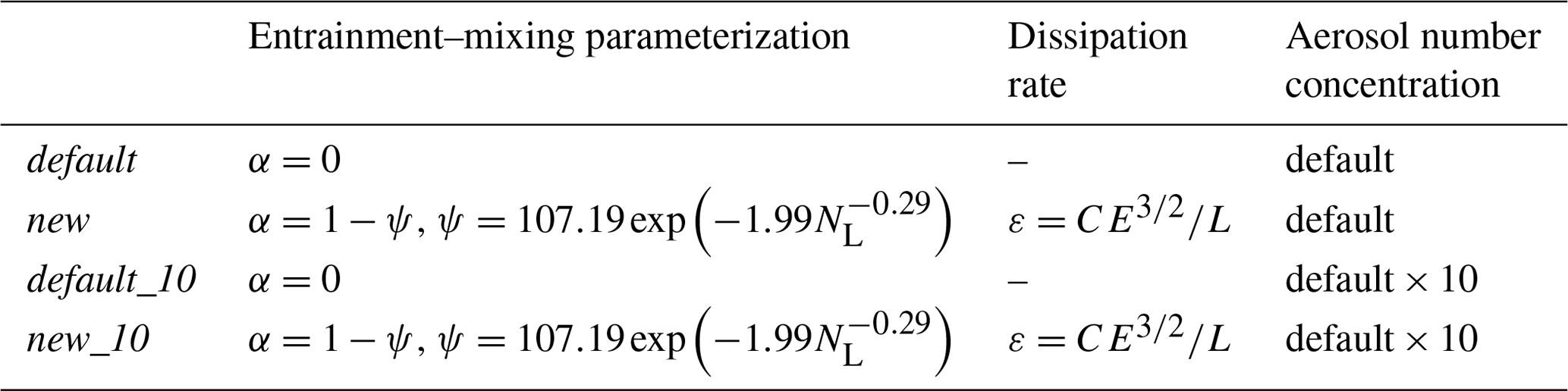
For each cloud case, ψ is first set to 1 for the default experiment because most LES models assume a homogeneous entrainment–mixing mechanism. The simulation with the new entrainment–mixing parameterization (Eqs. 1–6) is hereafter referred to as new. First, NL is diagnosed for each grid, and ψ is then calculated using Eq. (6). Finally, the variation in Nc during entrainment–mixing is obtained using Eqs. (1) and (2a). To examine the influence of the aerosol number concentration on the entrainment–mixing process, we conduct the numerical experiments default_10 and new_10 by multiplying the initial aerosol number concentrations for the default and new models, respectively, by a factor of 10. Thus, four sets of numerical experiments are conducted for both the cumulus and stratocumulus cases; the names of the experiments and corresponding descriptions are summarized in Table 1.
3.1 Cumulus case
For the cumulus case, the simulation starts at 12:00 UTC on 11 June 2016 and ends at 03:00 UTC on 12 June 2016 with an output interval of 10 min and spin times of 3 h. To demonstrate the utility of the model, Fig. 2 compares the temporal evolution of the observed and simulated cloud fraction (Fig. 2a) and solar irradiance (Fig. 2b) from the default experiment. Grid points with qc larger than 0.01 g kg−1 are defined as “cloudy areas”. Also shown for comparison are observational data with a 1 h temporal resolution, which are provided by the LES Atmospheric Radiation Measurement Symbiotic Simulation and Observation (LASSO) campaign (Gustafson et al., 2020). The observations show that the cloud forms at 12:00 UTC on 11 June and dissipates completely by 01:00 UTC on 12 June with a maximum cloud fraction of 0.47 at 16:00 UTC on 11 June. Considering the difference between the solar irradiances obtained from point measurements and the value representing the simulation domain, the observed solar irradiance at the Southern Great Plains (SGP) Central Facility are compared with the results of the central grid point in simulation (Fig. 2b). Evidently, although the results of the simulation do not fluctuate as much as the observations, the model captures the general behaviors of both cloud fraction and solar irradiance. The general agreement between the simulations and observations lends credence to using the model in further study.

Figure 2Time series of (a) domain-averaged cloud fraction and (b) total downward irradiance at the central point from the observation and the default experiment in the cumulus case.
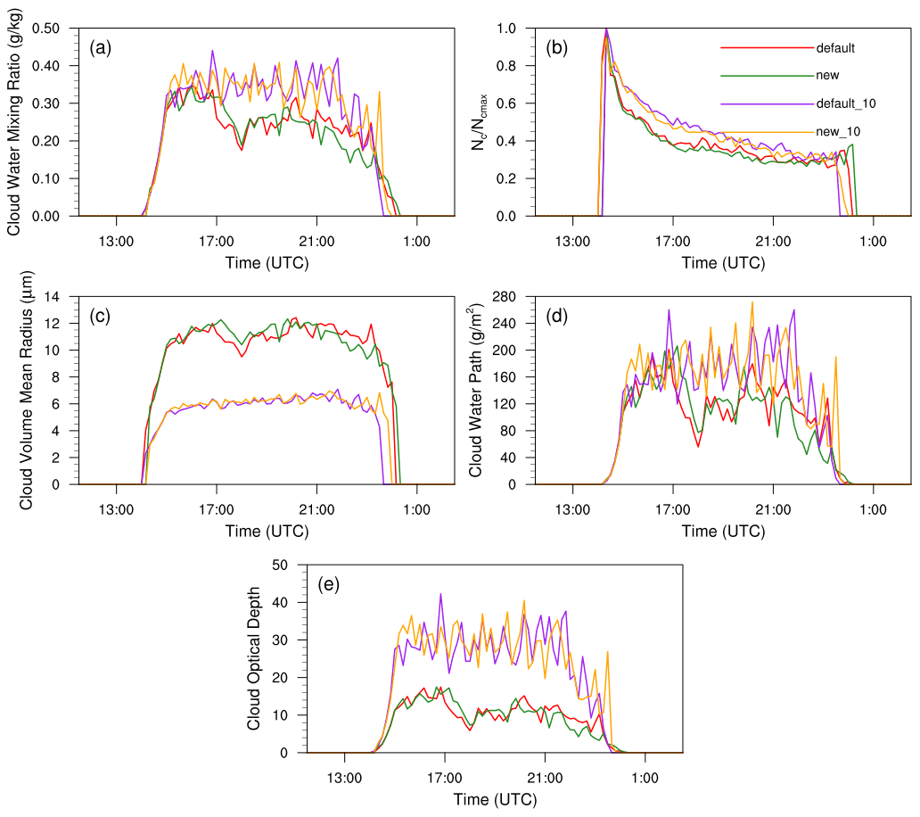
Figure 3The temporal evolutions of main cloud microphysical and optical properties in all simulation experiments for the cumulus case, including (a) cloud water mixing ratio (qc) (g kg−1), (b) cloud droplet number concentration (Nc) (cm−3), (c) cloud droplet volume mean radius (rv) (µm), (d) cloud water path (CWP) (g m−2), and (e) cloud optical depth (τ). In (b), Nc values in the experiments default and new are normalized by the maximum cloud droplet concentration (Ncmax) from default; Nc values in the experiments default_10 and new_10 are normalized by Ncmax from default_10. The four experiments are detailed in Table 1.
Figure 3 shows the evolution of the microphysical and optical properties of clouds in the cloudy areas of all simulation experiments, including qc, Nc, droplet volume mean radius (rv), cloud water path (CWP), and cloud optical depth (τ). To visually and simultaneously compare the change in cloud droplet concentration under different aerosol concentrations, the maximum cloud droplet concentration (Ncmax) from default is used to normalize Nc in default and new, while Ncmax from new_10 is used to normalize Nc in default_10 and new_10. The CWP is calculated as follows:
where ρa is the air density, qc(z) is the cloud water mixing ratio at each height (z), and H is the cloud thickness. The optical depth τ is estimated with
where ρw is the water density, and re(z) is the effective radius of the cloud droplets at each height (z). The time-averaged values of these physical properties of the clouds are listed in Table 2 for convenience.
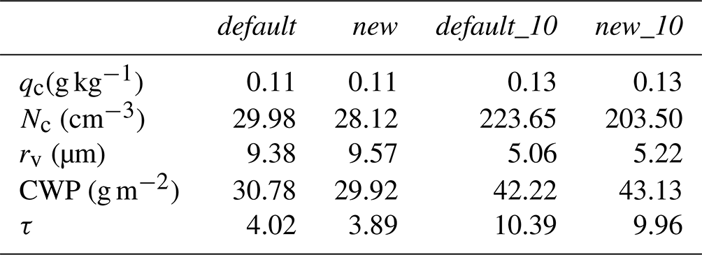
Table 2Summary of the case mean values of the key quantities in all the simulations of the cumulus case, containing cloud water mixing ratio (qc), cloud droplet number concentration (Nc), cloud droplet volume mean radius (rv), cloud water path (CWP), and cloud optical depth (τ). The experiments are detailed in Table 1.
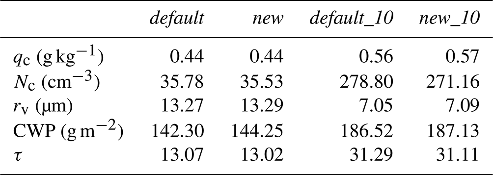
For the low aerosol number concentration, the simulations with the new entrainment–mixing parameterization have smaller Nc (35.53 cm−3) and larger rv (13.29 µm) than the default homogeneous simulation (35.78 cm−3 for Nc and 13.27 µm for rv in default). However, comparing new to default, the relative changes in Nc, rv, and τ are very small. When the aerosol concentration increases 10-fold (default_10 and new_10), qc, CWP, and τ increase according to the aerosol indirect effect (Peng et al., 2002; Wang et al., 2019; Li et al., 2011; Wang et al., 2011). Meanwhile, rv decreases significantly owing to the larger cloud number concentration. The effects of the new entrainment–mixing parameterization also increase; for example, the change in Nc increases from −0.70 % (new compared to default) to −2.74 % (new_10 compared to default_10), rv increases from +0.15 % to +0.57 %, and τ increases from −0.38 % to −0.58 %; the reasons for these changes are discussed later. These small changes are similar to those identified in previous cumulus studies (Jarecka et al., 2013; Hoffmann et al., 2019).
3.2 Stratocumulus case
The stratocumulus case is simulated from 09:00 UTC on 19 April 2009 to 03:00 UTC on 20 April 2009; the first 3 h are set to be spin-up times. We examine the stratocumulus region of the cloud base at ∼ 2.1 km and the cloud top at ∼ 2.3 km (cloud thickness of ∼ 200 m). Figure 4 shows the time series of the domain-averaged cloud fraction and total downward irradiance at the central point in the observation and the default experiment from 12:00 to 24:00 UTC. Similar to the cumulus case, the simulations compare favorably with the observations, which further reinforces the utility of the LES model. The observed data show that the cloud fraction increases with time and peaks at 16:00 UTC. The simulated cloud fraction has a value of 1 before 16:00 UTC, fluctuates from 16:00 to 21:00 UTC, and decreases sharply after 21:00 UTC. This period can be divided into three stages, namely the mature stage, pre-dissipation stage, and dissipation stage.
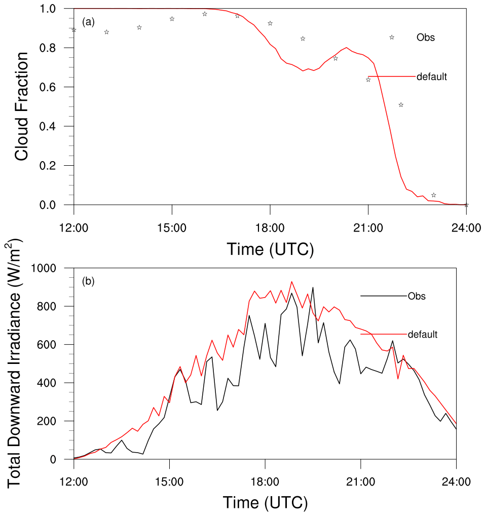
Figure 4Time series of (a) domain-averaged cloud fraction and (b) total downward irradiance at the central point from the observation and the default experiment in the stratocumulus case.
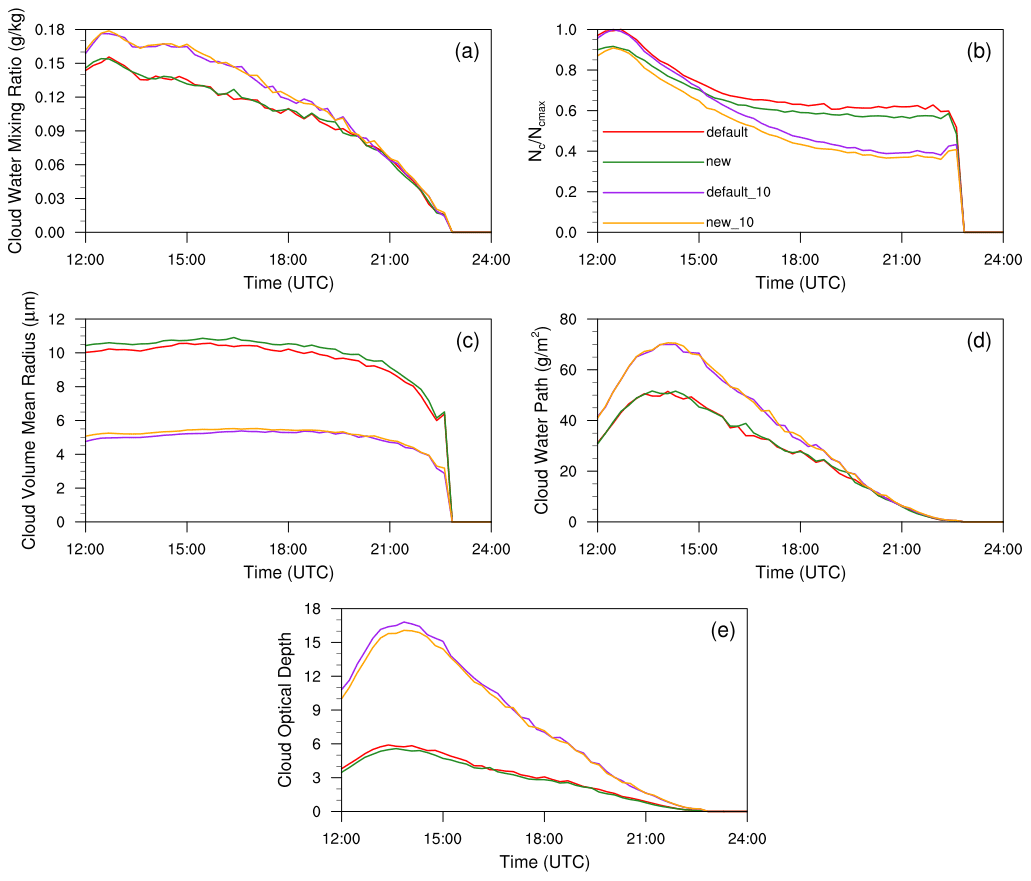
Figure 5The temporal evolutions of main cloud microphysical and optical properties in all simulation experiments for the stratocumulus case, including (a) cloud water mixing ratio (qc) (g kg−1), (b) cloud droplet number concentration (Nc) (cm−3), (c) cloud droplet volume mean radius (rv) (µm), (d) cloud water path (CWP) (g m−2), and (e) cloud optical depth (τ). In (b), Nc values in the experiments default and new are normalized by the maximum cloud droplet number concentration (Ncmax) from default; Nc values in the experiments default_10 and new_10 are normalized by Ncmax from default_10. The four experiments are detailed in Table 1.
As with the cumulus case, the temporal evolutions of the physical properties (qc, Nc, rv, CWP, and τ) of the clouds are shown in Fig. 5. In contrast to the oscillating changes exhibited by the physical quantities in the cumulus case (Fig. 3), the physical properties in the stratocumulus case exhibit a mostly smooth temporal evolution. Furthermore, default and new exhibit clear distinctions during the early periods, but these differences decrease during the dissipation stage. This is also the case with default_10 and new_10.
Table 3Summary of the case mean values of the key quantities in all the simulations of the stratocumulus case, including cloud water mixing ratio (qc), cloud droplet number concentration (Nc), cloud droplet volume mean radius (rv), cloud water path (CWP), and cloud optical depth (τ). The numbers in and out of the parentheses are the results at the mature and dissipation stages, respectively. The experiments are detailed in Table 1.

To compare the different behaviors of the simulation experiments at different stages, the results at the mature and dissipation stages are analyzed in detail. The mean values of the main microphysical and optical properties of the clouds are summarized in Table 3. As expected, the cloud microphysical and optical properties at the mature stage are all larger than those at the dissipation stage. The effects of the new entrainment–mixing parametrization are also more significant at the mature stage. Compared to default, the new model results in a 7.36 % smaller Nc, 3.20 % larger rv, and 5.98 % smaller τ during the mature stage. During the dissipation stage, the changes in Nc, rv, and τ are −4.76 %, +2.12 %, and −2.56 %, respectively. The largest influence of the new entrainment–mixing parametrization occurs during the mature stage when the aerosol concentration is 10 times greater. The differences in Nc, rv, and τ between new_10 and default_10 are −9.69 %, +3.88 %, and −5.85 %, respectively, averaged over the mature stage. These differences are much larger than those reported by Hill et al. (2009), who found that assuming extremely inhomogeneous mixing has a negligible effect on stratocumulus simulations. Our results also prove the speculation of Hill et al. (2009) that the mixing process might play an important role when the stratocumulus is thin (∼ 200 m in this study). Furthermore, implementing the new entrainment–mixing parameterization has similar effects on cloud properties to those described by Hoffmann and Feingold (2019), who used the linear eddy model to represent subgrid-scale turbulent mixing. Note that stratocumulus clouds occur in most regions around the world and are important contributors to the surface radiation budget (Wood, 2012; Zheng et al., 2016; Wang et al., 2021; Wang and Feingold, 2009). Stratocumulus clouds dominate in some regions and occur over 60 % of the time as vast long-lived sheets, such as the semipermanent subtropical marine stratocumulus sheets (Wood, 2012). In these regions, a nearly 6 % decrease in τ caused by the new entrainment–mixing parameterization is expected to have significant effects on the simulation of regional radiative properties and climate change.
The averaged influences of the new entrainment–mixing parametrization over all the simulation periods are also examined (Table 4). Quantitatively, the effect of the new entrainment–mixing parameterization is much greater on stratocumulus clouds than on cumulus clouds. Compared to default, new has an average change of −6.20 % in Nc, +2.01 % in rv, and −3.23 % in τ. When the aerosol concentration increases 10-fold, the differences in Nc, rv, and τ between default_10 and new_10 are −9.00 %, +3.16 %, and −4.14 %, respectively. These differences are larger than the largest changes in the cumulus case.
Table 4Cloud water mixing ratio (qc), cloud droplet number concentration (Nc), cloud droplet volume mean radius (rv), cloud water path (CWP), and cloud optical depth (τ) in all simulations for the entire lifetime of the stratocumulus case. The experiments are detailed in Table 1.
3.3 Mechanisms of the effects of the new entrainment–mixing parameterization
The different effects of the new entrainment–mixing parameterization on different types of clouds and even on different stages of stratocumulus clouds are likely be related to variations in the dominant mixing mechanism. To confirm this, we calculate the average ψ at all grid points experiencing evaporation, the proportion of inhomogeneous mixing grid points to all grid points experiencing evaporation, and the average ψ at the inhomogeneous mixing grid points in new and new_10 (Table 5) for the cumulus case, as well as the mature and dissipation stages in the stratocumulus case.
Table 5Homogeneous mixing degree (ψ) at all grid points experiencing evaporation, the proportion of inhomogeneous mixing grid points to all grid points experiencing evaporation, and ψ at the inhomogeneous mixing grid points in the experiments new and new_10 (Table 1) for the cumulus (Cu) and stratocumulus (St) cases. The numbers in and out of the parentheses are the results at the mature and dissipation stages in the stratocumulus (St) case, respectively. The experiments are detailed in Table 1.
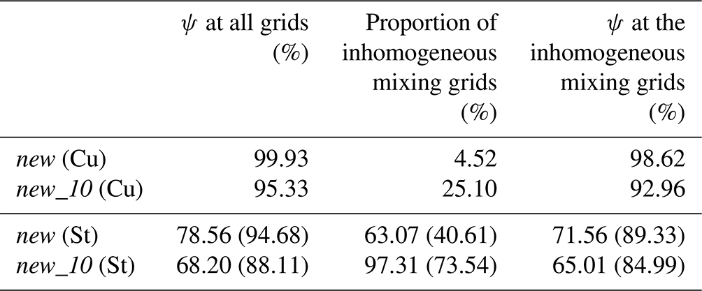
For the cumulus case, simulations exhibit large ψ and a small proportion of inhomogeneous mixing, indicating that homogeneous mixing is the dominant entrainment–mixing mechanism (Luo et al., 2020; Lu et al., 2013). Correspondingly, the influences of the new entrainment–mixing parameterization on the cloud physical properties are not significant, as shown in Fig. 3 and Table 2. The new_10 model exhibits a smaller average ψ and a larger proportion of inhomogeneous mixing than new, which results in larger changes in cloud physics, as mentioned in Sect. 3.1.
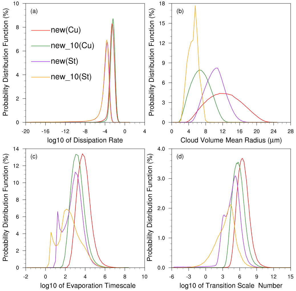
Figure 6Probability distribution functions (PDFs) of (a) turbulence dissipation rate (ε), (b) cloud droplet volume mean radius (rv), (c) evaporation timescale (τevap), and (d) transition scale number (NL) of cloud grids experiencing the entrainment–mixing process in the simulations with the new entrainment–mixing parameterization for the cumulus case (Cu, the solid lines) and the stratocumulus case (St, the dashed lines), respectively. The experiments are detailed in Table 1.
For the stratocumulus case, Table 5 shows the average ψ at all grid points experiencing evaporation, the proportion of inhomogeneous mixing grid points to all grid points experiencing evaporation, and the average ψ at the inhomogeneous mixing grid points during the two stages. The mature stage always has a smaller ψ but a larger proportion of inhomogeneous mixing than the dissipation stage. The inhomogeneous mixing process dominates the mature stage in new because more than 60 % of the grid points experience inhomogeneous mixing. The inhomogeneous mixing process is more dominant in new_10 because less than 3 % of the cloudy grid points experience a homogeneous mixing process during the mature stage, which explains why new_10 has the largest influence when implementing the new entrainment–mixing parametrization. Meanwhile, the average ψ in both stages is smaller than that in the cumulus case for the same simulation configuration. Thus, the effects of the new entrainment–mixing parameterization are more significant for stratocumulus than for cumulus clouds, especially at the mature stage. It is noted that the average ψ and the proportion of inhomogeneous mixing at the dissipation stage of new in the stratocumulus case are very close to the results of new_10 in the cumulus case. This is because the cloud fraction decreases sharply during the dissipation stage; the stratocumulus clouds break up and produce cumulus clouds with small cloud droplet radii.
3.4 The effects of dissipation rate and aerosol concentration on the entrainment–mixing process
Previous studies have shown the notable effects of the dissipation rate and aerosol concentration on the entrainment–mixing process. For example, Luo et al. (2020) changed ε from 10−5 to 10−2 m2 s−3 and noted huge differences in the corresponding ψ. Small et al. (2013) compared aircraft observations with different background concentrations and found that higher-pollution flights tended to slightly more inhomogeneous mixing; Jarecka et al. (2013) also showed various homogeneities of subgrid mixing when aerosol concentration increases 10-fold. To explain the different behaviors of different simulations with the new entrainment–mixing parameterization, the influences of ε and aerosol concentration are examined. Figure 6 shows the probability distribution functions (PDFs) of ε, rv, τevap, and NL for cloud grids experiencing entrainment–mixing processes in new and new_10 for the cumulus and stratocumulus cases, respectively. The PDFs from the mature and dissipation stages of the stratocumulus case are shown in Fig. 7.
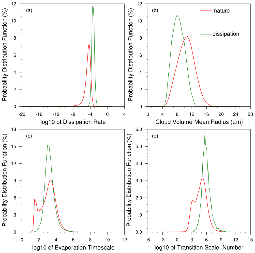
Figure 7Probability distribution functions (PDFs) of (a) turbulence dissipation rate (ε), (b) cloud droplet volume mean radius (rv), (c) evaporation timescale (τevap), and (d) transition scale number (NL) of cloud grids experiencing the entrainment–mixing process at the mature stage from 12:00 to 16:00 UTC (the red lines) and the dissipation stage from 21:00 to 24:00 UTC (the green lines) in new for the stratocumulus case. The experiment is detailed in Table 1.
3.4.1 Dissipation rate
According to Eq. (3), NL is a function of ; hence, the PDF of ε directly affects NL and further results in different ψ. For the cumulus case, the mean ε of 0.0043 m2 s−3 in new is similar to those obtained for cumulus clouds in previous studies (e.g. Lu et al., 2016; Hoffmann et al., 2019). As shown in Fig. 1, cloud grids experience a homogeneous mixing process if NL is larger than ∼ 105, the limited distribution of NL values less than 105 in new results in a very small number of cloud grid points undergoing an inhomogeneous mixing process. Even at the cloud grid points that undergo inhomogeneous mixing, the average ψ is large (98.62 %) because most of the NL values are larger than 103. Therefore, the cloud properties in new are close to those in default.
For the stratocumulus case, the mean value of ε (2.9 × 10⁻⁴ m2 s−3 in new) is an order of magnitude less than those in the cumulus case. Therefore, compared with the cumulus case, NL is reduced in the stratocumulus case, while the peak value of new almost reaches the criterion of inhomogeneous mixing (∼ 105). For the two stages of stratocumulus clouds, ε is an order of magnitude smaller, but rv was larger (Fig. 7) during the mature stage than during the dissipation stage. According to Eq. (5a), droplets with smaller rv are more prone to complete evaporation and have a smaller τevap. The combination of smaller ε and larger rv results in a smaller NL (Eq. 3). This is the reason for the new entrainment–mixing parametrization having more significant effects during the mature stage than during the dissipation stage. In addition, the similarity of the ε and rv values during the dissipation stage of the stratocumulus case in new, compared to the cumulus case in new_10 (Fig. 6a and b), explains the similar average ψ values of these scenarios and the proportion of inhomogeneous mixing (Table 5).
Therefore, the distribution of ε has a vital impact on the influence of the new entrainment–mixing parameterization. Smaller values of ε result in the new entrainment–mixing parameterization having a more significant influence. Moreover, the rv in the stratocumulus case is smaller than that in the cumulus case, which is also conducive to a more inhomogeneous mixing process. These are the reasons why the implementation of the new entrainment–mixing parameterization has a larger influence in the stratocumulus case than in the cumulus case when compared to a homogeneous mixing mechanism.
3.4.2 Aerosol concentration
The aerosol concentration affects the entrainment–mixing process by decreasing the cloud droplet radius. As rv decreases, the distributions of τevap in new_10 move to a smaller overall value, while the mean value is an order of magnitude smaller than that in new, which causes a much smaller NL because NL is proportional to (Eqs. 3a and 3b). The larger percentage of smaller NL values indicates that in new_10, more grid points undergo an inhomogeneous mixing process, and the proportion of such grid points is much larger than in the new model (Table 5). Therefore, compared to new, new_10 exhibits a smaller ψ, and the effects of the new entrainment–mixing parameterization on cloud properties are more obvious for both the cumulus and stratocumulus cases.
3.5 Verification by the simulations with a different parameterization using entrained air relative humidity
In the above simulations, the new entrainment–mixing parameterization is based on the grid mean RH. This section serves to verify these simulations using the entrainment–mixing parameterization proposed by Luo et al. (2020),
which was developed using the entrained air RH in the EMPM. This parameterization needs the entrained air RH within each grid in WRF, which is estimated following Grabowski (2007) and Jarecka et al. (2009). Briefly, assuming that RH mixes linearly when the dry air entrains into the cloud, then entrained air RH can be simply calculated by
where the subscripts entrained, cloud, and grid indicate the RH of the entrained, cloudy, and grid point air, respectively. In Eq. (10), although the cloudy air RH is approximately 100 % and grid mean RH is predicted in the model, the entrained air fraction f needs to be further parameterized. To obtain f at 100 m, a parameterization of f is developed based on the simulations for both the cumulus and stratocumulus cases with a higher resolution of 10 m; the other configurations are the same as those in the experiment default. The 10 m resolution simulation results are then averaged to the resolution of 100 m. Following Xu and Randall (1996), “1−f” can be fitted by the function
where γ and β are empirical parameters. Figure 8 shows that the parameterization with γ=8.72 and β=1.47 × 10⁴ can reproduce well the simulated values of “1−f”, with the correlation coefficient (R) of 0.89 and significant level p value < 0.01. Considering that local shear () and buoyancy (B) may drive turbulence generation and entrainment for a microscale process, the two quantities are also used to fit “1−f” except for RHgrid and qc. However, the addition of and B to Eq. (11) does not increase R. Therefore, using RHgrid and qc to parametrize “1−f” is good and reasonable for a microscale process.
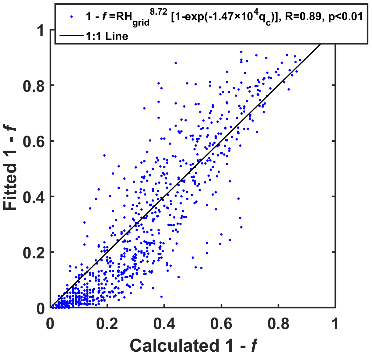
Figure 8The fitted 1−f as a function of the calculated 1−f. The fitted 1−f is obtained by the fitting functions with grid mean relative humidity (RHgrid) and cloud water mixing ratio (qc). The black line denotes the 1 : 1 line.
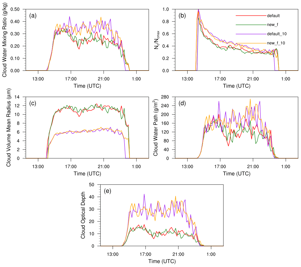
Figure 9The temporal evolutions of main cloud microphysical and optical properties in all simulation experiments for the cumulus case, including (a) cloud water mixing ratio (qc) (g kg−1), (b) cloud droplet number concentration (Nc) (cm−3), (c) cloud droplet volume mean radius (rv) (µm), (d) cloud water path (CWP) (g m−2), and (e) cloud optical depth (τ). In (b), Nc values in the experiments default and new_f are normalized by the maximum cloud droplet concentration (Ncmax) from default; Nc values in the experiments default_10 and new_f_10 are normalized by Ncmax from default_10; new_f and new_f_10 are the experiments using entrained air relative humidity.
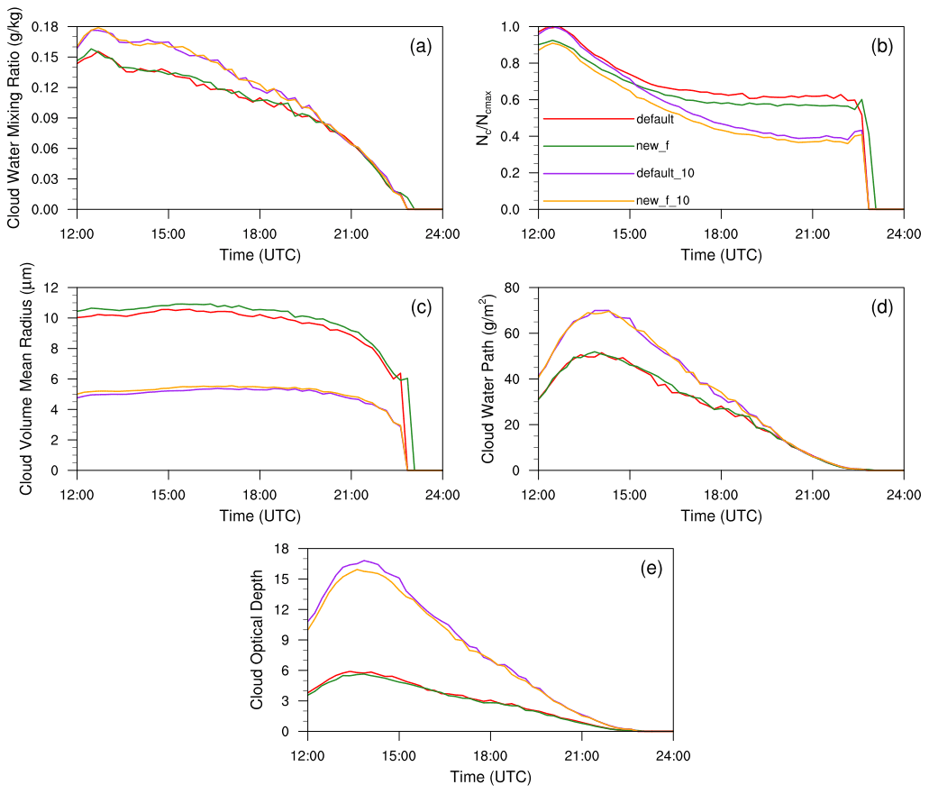
Figure 10The temporal evolutions of main cloud microphysical and optical properties in all simulation experiments for the stratocumulus case, including (a) cloud water mixing ratio (qc) (g kg−1), (b) cloud droplet number concentration (Nc) (cm−3), (c) cloud droplet volume mean radius (rv) (µm), (d) cloud water path (CWP) (g m−2), and (e) cloud optical depth (τ). In (b), Nc values in the experiments default and new are normalized by the maximum cloud droplet number concentration (Ncmax) from default; Nc values in the experiments default_10 and new_10 are normalized by Ncmax from default_10; new_f and new_f_10 are the experiments using entrained air relative humidity.
Table 6Cloud water mixing ratio (qc), cloud droplet number concentration (Nc), cloud droplet volume mean radius (rv), cloud water path (CWP), and cloud optical depth (τ) in new_f and new_f_10 for the cumulus (Cu) and stratocumulus (Sc) cases. The results of new and new_10 in Tables 2 and 4 are shown in the parentheses.
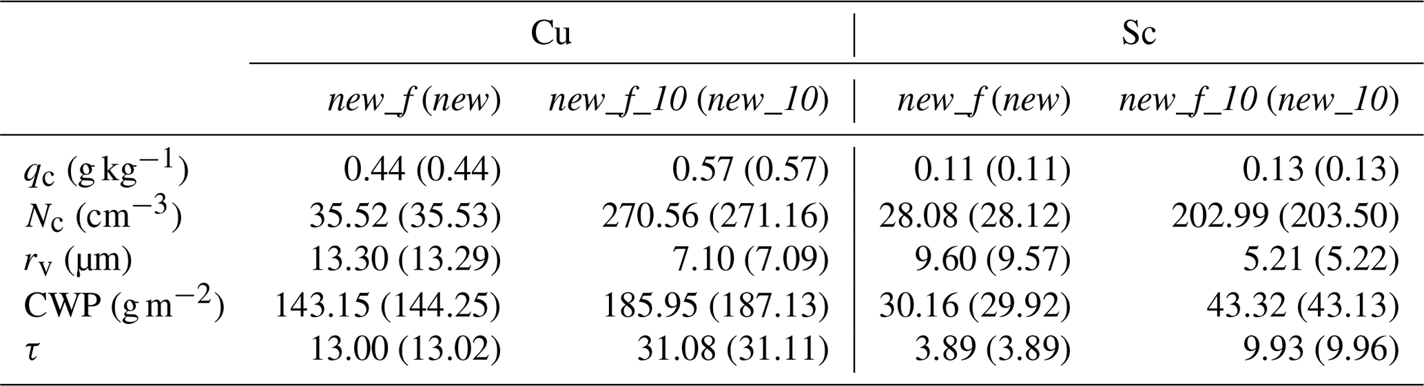
Equations (9)–(11) are applied in the simulations for both the cumulus and stratocumulus cases with different aerosol background (hereafter new_f and new_f_10). The same as for Figs. 3 and 5, the temporal evolutions of the cloud physical properties (qc, Nc, rv, CWP, and τ) in default, default_10, new_f, and new_f_10 are shown in Figs. 9 and 10. The results are similar to Figs. 3 and 5. The mean values of these properties of new_f and new_f_10 for the cumulus and stratocumulus cases are also shown in Table 6, and the results of new and new_10 are also shown in the parentheses for the convenience of comparison. The results of new_f and new are very similar, with the maximum difference being no more than 1 %, and so are the results of 10-fold aerosol background. Such a close agreement suggests that the results of the new entrainment–mixing parametrization with grid mean RH are reliable.
It is worth noting that instead of parameterizing f, Jarecka et al. (2009, 2013) added an equation to predict f for each grid. In principle, this is a good choice if this method is available in models. Our method shown here is an alternative way to represent the entrainment–mixing process when the prognostic f is not available.
The entrainment–mixing process near cloud edges has important effects on cloud microphysics, but the most commonly used microphysics schemes simply assume one extreme mechanism, that is, homogeneous entrainment–mixing. This study first improves the entrainment–mixing parameterization proposed by Luo et al. (2020), which connects the homogeneous mixing degree and transition scale number to estimate the homogeneity of the subgrid mixing process and its impact on the droplet number concentration. The improved parameterization uses grid mean relative humidity and can be implemented directly into microphysics schemes; there is no need to know the relative humidity of the entrained air. Second, the modified entrainment–mixing parameterization is implemented in the two-moment Thompson aerosol-aware scheme of the LES version of WRF-Solar to examine its effects on the microphysical and optical properties of cumulus and stratocumulus clouds. Third, several sensitivity experiments are conducted to investigate the effects of the new entrainment–mixing parameterization under different conditions of turbulence dissipation rate and aerosol number concentration. The results of implementing the new entrainment–mixing parameterization are finally verified by the results using entrained air properties.
Unlike the commonly assumed homogeneous mixing scenario, the new entrainment–mixing parameterization produces a smaller cloud droplet number concentration and larger cloud droplet radius, with the degree of difference depending on cloud types and stages. Sensitivity tests show that in the cumulus case, the largest average influence of the new entrainment–mixing parameterization occurs under a high aerosol background but results in only a 2.74 % decrease in cloud droplet number concentration and a 0.57 % increase in cloud droplet volume mean radius. The changes become even smaller with a low aerosol background because of the larger cloud droplet radius. In contrast, the new entrainment–mixing parameterization has a larger influence on the microphysical and optical properties of stratocumulus clouds, especially under a high aerosol background and during the mature stage, with a cloud fraction equal to 1. The largest changes resulting from the new entrainment–mixing parameterization are −9.69 %, +3.88 %, and −5.85 % for cloud number concentration, cloud droplet volume mean radius, and cloud optical depth, respectively. The new entrainment–mixing parameterization has less of an influence on the dissipation stage than on the mature stage of the stratocumulus case but affects this case more than the cumulus case.
The varying effects of the new entrainment–mixing parameterization are caused by variations in the dominant entrainment–mixing mechanism between different cloud types and stages. Compared to the cumulus case, the stratocumulus case has a much smaller homogeneous mixing degree and a larger proportion of inhomogeneous mixing grid points, especially during the mature stage, which indicates that the inhomogeneous mixing mechanism dominates in the stratocumulus case, while the homogeneous mixing mechanism dominates in the cumulus case. As mentioned above, the changes in physical properties of stratocumulus clouds in the dissipation stage are between those in the mature stage and those of the cumulus case; this is because stratocumulus clouds dissipate sharply to form small cumulus clouds, and the degree of homogeneous mixing during the dissipation stage is therefore between that which occurs during the mature stage and the cumulus case.
Sensitivity studies show that turbulence dissipation rate and aerosol concentration can have notable effects on the subgrid homogeneity of the mixing process. A larger dissipation rate can accelerate the mixing process, which results in a larger transition scale number and homogeneous mixing degree and, therefore, a mostly homogenous mixing mechanism. This is why the cumulus case exhibits smaller changes than the stratocumulus case after the new entrainment–mixing parameterization is implemented. Larger aerosol number concentrations cause a smaller cloud droplet radius. Smaller droplets evaporate more easily, which leads to a smaller transition scale number and a smaller homogeneous mixing degree. Thus, the entrainment–mixing mechanism tends to be inhomogeneous. Therefore, a larger aerosol number concentration increases the influence of the new entrainment–mixing parameterization in both the cumulus and stratocumulus cases.
The influences of implementing the new entrainment–mixing parameterization with grid mean relative humidity have been verified by simulations with entrained air properties. The entrained air properties are obtained and calculated from simulations with a finer resolution (10 m). Sensitivity tests show similar cloud microphysical and optical properties in the two different methods, which suggests that the new entrainment–mixing parameterization with grid mean relative humidity is convincing.
Note that the new entrainment–mixing parameterization could be more important in the models if the relative humidity near the cloud is more accurately simulated because numerical diffusion may spuriously humidify the entrained air (Hoffmann and Feingold, 2019). The artificially increased relative humidity limits the influences of the new entrainment–mixing parameterization because homogeneous and inhomogeneous entrainment–mixing processes are close to each other under conditions of high relative humidity.
The large-scale forcing data used in this study can be downloaded from Atmospheric Radiation Measurement (ARM) user facility (https://doi.org/10.5439/1647300, Tao and Xie, 2004; https://doi.org/10.5439/1647174, Tao and Xie, 2012). The LASSO data can be downloaded from https://doi.org/10.5439/1342961 (Gustafson et al., 2017).
XX, CL, and YL designed the experiments. XX carried out the experiments and conducted the data analysis with contributions from all coauthors. XX, CL, XZ, and SE developed the model code. XX prepared the paper with help from CL, YL, YW, SL, and LZ.
The contact author has declared that neither they nor their co-authors have any competing interests.
The views expressed herein do not necessarily represent the views of the U.S. Department of Energy or the United States Government.
Publisher's note: Copernicus Publications remains neutral with regard to jurisdictional claims in published maps and institutional affiliations.
This research is supported by the National Natural Science Foundation of China (41822504, 42175099, 42027804, 41975181, 42075073). Yangang Liu, Xin Zhou, and Satoshi Endo are supported by the U.S. Department of Energy's Office of Energy Efficiency and Renewable Energy (EERE) under Solar Energy Technologies Office (SETO) award number 33504, as well as the Office of Science Biological and Environmental Research program as part of the Atmospheric Systems Research (ASR) program. Brookhaven National Laboratory is operated by Battelle for the U.S. Department of Energy under contract DE-SC00112704.
This research has been supported by the National Natural Science Foundation of China (grant nos. 41822504, 42175099, 42027804, 41975181, and 42075073) and the U.S. Department of Energy (Solar Energy Technologies Office (SETO), award number 33504; Atmospheric System Research (ASR) program, grant no. DE-SC00112704).
This paper was edited by Hailong Wang and reviewed by two anonymous referees.
Ackerman, A. S., Kirkpatrick, M. P., Stevens, D. E., and Toon, O. B.: The impact of humidity above stratiform clouds on indirect aerosol climate forcing, Nature, 432, 1014–1017, 2004.
Andrejczuk, M., Grabowski, W. W., Malinowski, S. P., and Smolarkiewicz, P. K.: Numerical simulation of cloud-clear air interfacial mixing: Effects on cloud microphysics, J. Atmos. Sci., 63, 3204–3225, https://doi.org/10.1175/JAS3813.1, 2006.
Andrejczuk, M., Grabowski, W. W., Malinowski, S. P., and Smolarkiewicz, P. K.: Numerical simulation of cloud–clear air interfacial mixing: Homogeneous versus inhomogeneous mixing, J. Atmos. Sci., 66, 2493–2500, https://doi.org/10.1175/2009JAS2956.1, 2009.
Burnet, F. and Brenguier, J. L.: Observational study of the entrainment-mixing process in warm convective clouds, J. Atmos. Sci., 64, 1995–2011, https://doi.org/10.1175/JAS3928.1, 2007.
Chosson, F., Brenguier, J.-L., and Schüller, L.: Entrainment-mixing and radiative transfer simulation in boundary layer clouds, J. Atmos. Sci., 64, 2670–2682, https://doi.org/10.1175/JAS3975.1, 2007.
Deardorff, J.: Stratocumulus-capped mixed layers derived from a three-dimensional model, Bound.-Lay. Meteorol., 18, 495–527, https://doi.org/10.1007/BF00119502, 1980.
Del Genio, A. D. and Wu, J.: The role of entrainment in the diurnal cycle of continental convection, J. Climate, 23, 2722–2738, https://doi.org/10.1175/2009JCLI3340.1, 2010.
Endo, S., Fridlind, A. M., Lin, W., Vogelmann, A. M., Toto, T., Ackerman, A. S., McFarquhar, G. M., Jackson, R. C., Jonsson, H. H., and Liu, Y.: RACORO continental boundary layer cloud investigations: 2. Large-eddy simulations of cumulus clouds and evaluation with in situ and ground-based observations, J. Geophys. Res.-Atmos., 120, 5993–6014, 2015.
Fan, J., Wang, Y., Rosenfeld, D., and Liu, X.: Review of Aerosol–Cloud Interactions: Mechanisms, Significance, and Challenges, J. Atmos. Sci., 73, 4221–4252, https://doi.org/10.1175/jas-d-16-0037.1, 2016.
Freud, E., Rosenfeld, D., Andreae, M. O., Costa, A. A., and Artaxo, P.: Robust relations between CCN and the vertical evolution of cloud drop size distribution in deep convective clouds, Atmos. Chem. Phys., 8, 1661–1675, https://doi.org/10.5194/acp-8-1661-2008, 2008.
Freud, E., Rosenfeld, D., and Kulkarni, J. R.: Resolving both entrainment-mixing and number of activated CCN in deep convective clouds, Atmos. Chem. Phys., 11, 12887–12900, https://doi.org/10.5194/acp-11-12887-2011, 2011.
Gao, S., Lu, C., Liu, Y., Mei, F., Wang, J., Zhu, L., and Yan, S.: Contrasting Scale Dependence of Entrainment-Mixing Mechanisms in Stratocumulus Clouds, Geophys. Res. Lett., 47, e2020GL086970, https://doi.org/10.1029/2020gl086970, 2020.
Gao, S., Lu, C., Liu, Y., Yum, S. S., Zhu, J., Zhu, L., Desai, N., Ma, Y., and Wu, S.: Comprehensive quantification of height dependence of entrainment mixing between stratiform cloud top and environment, Atmos. Chem. Phys., 21, 11225–11241, https://doi.org/10.5194/acp-21-11225-2021, 2021.
Gao, Z., Liu, Y., Li, X., and Lu, C.: Investigation of Turbulent Entrainment-Mixing Processes with a New Particle-Resolved Direct Numerical Simulation Model, J. Geophys. Res., 123, 2194–2214, 2018.
Gerber, H. E., Frick, G. M., Jensen, J. B., and Hudson, J. G.: Entrainment, mixing, and microphysics in trade-wind cumulus, J. Meteorol. Soc. Jpn., 86A, 87–106, 2008.
Grabowski, W. W.: Indirect impact of atmospheric aerosols in idealized simulations of convective-radiative quasi equilibrium, J. Climate, 19, 4664–4682, https://doi.org/10.1175/JCLI3857.1, 2006.
Grabowski, W. W.: Representation of turbulent mixing and buoyancy reversal in bulk cloud models, J. Atmos. Sci., 64, 3666–3680, 2007.
Grabowski, W. W. and Morrison, H.: Indirect Impact of Atmospheric Aerosols in Idealized Simulations of Convective–Radiative Quasi Equilibrium. Part II: Double-Moment Microphysics, J. Climate, 24, 1897–1912, https://doi.org/10.1175/2010jcli3647.1, 2011.
Gustafson, W. I., Vogelmann, A. M., Li, Z., Cheng, X., Dumas, K. K., Endo, S., Johnson, K. L., Krishna, B., Fairless, T., and Xiao, H.: The Large-Eddy Simulation (LES) Atmospheric Radiation Measurement (ARM) Symbiotic Simulation and Observation (LASSO) Activity for Continental Shallow Convection, B. Am. Meteorol. Soc., 101, E462–E479, https://doi.org/10.1175/bams-d-19-0065.1, 2020.
Gustafson, W. I., Vogelmann, A. M., Cheng, X., Endo, S., Johnson, K. L., Krishna, B., Li, Z., Toto, T., and Xiao, H.: LASSO data bundles, Atmospheric Radiation Measurement user facility [data set], https://doi.org/10.5439/1342961, 2017.
Hacker, J. P., Jimenez, P. A., Dudhia, J., Haupt, S. E., Ruiz-Arias, J. A., Gueymard, C. A., Thompson, G., Eidhammer, T., and Deng, A.: WRF-Solar: Description and Clear-Sky Assessment of an Augmented NWP Model for Solar Power Prediction, B. Am. Meteorol. Soc., 97, 1249–1264, https://doi.org/10.1175/bams-d-14-00279.1, 2016.
Haman, K. E., Malinowski, S. P., Kurowski, M. J., Gerber, H., and Brenguier, J.-L.: Small scale mixing processes at the top of a marine stratocumulus – a case study, Q. J. Roy. Meteor. Soc., 133, 213–226, https://doi.org/10.1002/qj.5, 2007.
Haupt, S. E., Kosovic, B., Jensen, T., Lee, J., Jimenez, P., Lazo, J., Cowie, J., McCandless, T., Pearson, J., and Weiner, G.: The SunCast? solar-power forecasting system: the results of the public-private-academic partnership to advance solar power forecasting, National Center for Atmospheric Research (NCAR), Research Applications Laboratory, Weather Systems and Assessment Program (US), Boulder (CO), https://doi.org/10.5065/D6N58JR2, 2016.
Hill, A. A., Feingold, G., and Jiang, H.: The influence of entrainment and mixing assumption on aerosol-cloud interactions in marine stratocumulus, J. Atmos. Sci., 66, 1450–1464, 2009.
Hoffmann, F. and Feingold, G.: Entrainment and mixing in stratocumulus: Effects of a new explicit subgrid-scale scheme for large-eddy simulations with particle-based microphysics, J. Atmos. SCi., 76, 1955–1973, https://doi.org/10.1175/jas-d-18-0318.1, 2019.
Hoffmann, F., Yamaguchi, T., and Feingold, G.: Inhomogeneous mixing in Lagrangian cloud models: Effects on the production of precipitation embryos, J. Atmos. Sci., 76, 113–133, 2019.
Huang, J., Lee, X., and Patton, E. G.: A modelling study of flux imbalance and the influence of entrainment in the convective boundary layer, Bound.-Lay. Meteorol., 127, 273–292, 2008.
Jarecka, D., Grabowski, W. W., and Pawlowska, H.: Modeling of Subgrid-Scale Mixing in Large-Eddy Simulation of Shallow Convection, J. Atmos. Sci., 66, 2125–2133, https://doi.org/10.1175/2009jas2929.1, 2009.
Jarecka, D., Grabowski, W. W., Morrison, H., and Pawlowska, H.: Homogeneity of the subgrid-scale turbulent mixing in large-eddy simulation of shallow convection, J. Atmos. Sci., 70, 2751–2767, 2013.
Jensen, J. B., Austin, P. H., Baker, M. B., and Blyth, A. M.: Turbulent mixing, spectral evolution and dynamics in a warm cumulus cloud, J. Atmos. Sci., 42, 173–192, https://doi.org/10.1175/1520-0469(1985)042<0173:TMSEAD>2.0.CO;2, 1985.
Kim, B.-G., Miller, M. A., Schwartz, S. E., Liu, Y., and Min, Q.: The role of adiabaticity in the aerosol first indirect effect, J. Geophys. Res., 113, D05210, https://doi.org/10.1029/2007jd008961, 2008.
Kumar, B., Schumacher, J., and Shaw, R.: Cloud microphysical effects of turbulent mixing and entrainment, Theor. Comp. Fluid Dyn., 27, 361–376, 2013.
Lasher-Trapp, S. G., Cooper, W. A., and Blyth, A. M.: Broadening of droplet size distributions from entrainment and mixing in a cumulus cloud, Q. J. Roy. Meteor. Soc., 131, 195–220, https://doi.org/10.1256/qj.03.199, 2005.
Lehmann, K., Siebert, H., and Shaw, R. A.: Homogeneous and inhomogeneous mixing in cumulus clouds: dependence on local turbulence structure, J. Atmos. Sci., 66, 3641–3659, https://doi.org/10.1175/2009JAS3012.1, 2009.
Li, Z., Li, C., Chen, H., Tsay, S. C., Holben, B., Huang, J., Li, B., Maring, H., Qian, Y., and Shi, G.: East Asian studies of tropospheric aerosols and their impact on regional climate (EAST-AIRC): An overview, J. Geophys. Res.-Atmos., 116, D00K34, https://doi.org/10.1029/2010JD015257, 2011.
Lu, C., Liu, Y., and Niu, S.: Examination of turbulent entrainment-mixing mechanisms using a combined approach, J. Geophys. Res., 116, D20207, https://doi.org/10.1029/2011JD015944, 2011.
Lu, C., Liu, Y., Niu, S., Krueger, S., and Wagner, T.: Exploring parameterization for turbulent entrainment-mixing processes in clouds, J. Geophys. Res.-Atmos., 118, 185–194, https://doi.org/10.1029/2012jd018464, 2013.
Lu, C., Liu, Y., Niu, S., and Endo, S.: Scale dependence of entrainment-mixing mechanisms in cumulus clouds, J. Geophys. Res.-Atmos., 119, 13877–13890, 2014.
Lu, C., Liu, Y., Zhang, G. J., Wu, X., Endo, S., Cao, L., Li, Y., and Guo, X.: Improving parameterization of entrainment rate for shallow convection with aircraft measurements and large eddy simulation, J. Atmos. Sci., 73, 761–773, https://doi.org/10.1175/JAS-D-15-0050.1, 2016.
Luo, S., Lu, C., Liu, Y., Bian, J., Gao, W., Li, J., Xu, X., Gao, S., Yang, S., and Guo, X.: Parameterizations of Entrainment-Mixing Mechanisms and Their Effects on Cloud Droplet Spectral Width Based on Numerical Simulations, J. Geophys. Res.-Atmos., 125, e2020JD032972, https://doi.org/10.1029/2020JD032972, 2020.
Morrison, H. and Grabowski, W. W.: Modeling supersaturation and subgrid-scale mixing with two-moment bulk warm microphysics, J. Atmos. Sci., 65, 792–812, https://doi.org/10.1175/2007JAS2374.1, 2008.
Paluch, I. R. and Baumgardner, D. G.: Entrainment and fine-scale mixing in a continental convective cloud, J. Atmos. Sci., 46, 261–278, https://doi.org/10.1175/1520-0469(1989)046<0261:EAFSMI>2.0.CO;2, 1989.
Pawlowska, H., Brenguier, J. L., and Burnet, F.: Microphysical properties of stratocumulus clouds, Atmos. Res., 55, 15–33, 2000.
Peng, Y., Lohmann, U., Leaitch, R., Banic, C., and Couture, M.: The cloud albedo-cloud droplet effective radius relationship for clean and polluted clouds from RACE and FIRE.ACE, J. Geophys. Res., 107, AAC 1-1–AAC 1-6, https://doi.org/10.1029/2000JD000281, 2002.
Slawinska, J., Grabowski, W. W., Pawlowska, H., and Wyszogrodzki, A. A.: Optical properties of shallow convective clouds diagnosed from a bulk-microphysics large-eddy simulation, J. Climate, 21, 1639–1647, 2008.
Slawinska, J., Grabowski, W. W., Pawlowska, H., and Morrison, H.: Droplet activation and mixing in large-eddy simulation of a shallow cumulus field, J. Atmos. Sci., 69, 444–462, 2012.
Small, J. D., Chuang, P., and Jonsson, H.: Microphysical imprint of entrainment in warm cumulus, Tellus B, 65, 6647–6662, 2013.
Tao, C. and Xie, S.: Constrained Variational Analysis (60VARANARUC). 2004-01-01 to 2012-04-30, Southern Great Plains (SGP) Central Facility, Lamont, OK, ARM Data Center [data set], https://doi.org/10.5439/1647300, 2004.
Tao, C. and Xie, S.: Constrained Variational Analysis (60VARANARAP). 2012-05-01 to 2019-08-31, Southern Great Plains (SGP) Central Facility, Lamont, OK, ARM Data Center [data set], https://doi.org/10.5439/1647174, 2012.
Thompson, G. and Eidhammer, T.: A study of aerosol impacts on clouds and precipitation development in a large winter cyclone, J. Atmos. Sci., 71, 3636–3658, 2014.
Wang, H. and Feingold, G.: Modeling mesoscale cellular structures and drizzle in marine stratocumulus. Part I: Impact of drizzle on the formation and evolution of open cells, J. Atmos. Sci., 66, 3237–3256, 2009.
Wang, M., Ghan, S., Ovchinnikov, M., Liu, X., Easter, R., Kassianov, E., Qian, Y., and Morrison, H.: Aerosol indirect effects in a multi-scale aerosol-climate model PNNL-MMF, Atmos. Chem. Phys., 11, 5431–5455, https://doi.org/10.5194/acp-11-5431-2011, 2011.
Wang, Y., Niu, S., Lv, J., Lu, C., Xu, X., Wang, Y., Ding, J., Zhang, H., Wang, T., and Kang, B.: A new method for distinguishing unactivated particles in cloud condensation nuclei measurements: Implications for aerosol indirect effect evaluation, Geophys. Res. Lett., 46, 14185–14194, 2019.
Wang, Y., Zhao, C., McFarquhar, G. M., Wu, W., Reeves, M., and Li, J.: Dispersion of Droplet Size Distributions in Supercooled Non-precipitating Stratocumulus from Aircraft Observations Obtained during the Southern Ocean Cloud Radiation Aerosol Transport Experimental Study, J. Geophys. Res.-Atmos., 126, e2020JD033720, https://doi.org/10.1029/2020JD033720, 2021.
Wood, R.: Review: Stratocumulus Clouds, Mon. Weather Rev., 140, 2373–2423, 2012.
Xu, K.-M. and Randall, D. A.: A semiempirical cloudiness parameterization for use in climate models, J. Atmos. Sci., 53, 3084–3102, 1996.
Xu, X., Lu, C., Liu, Y., Gao, W., Wang, Y., Cheng, Y., Luo, S., and Van Weverberg, K.: Effects of cloud liquid-phase microphysical processes in mixed-phase cumuli over the Tibetan Plateau, J. Geophys. Res.-Atmos., 125, e2020JD033371, https://doi.org/10.1029/2020JD033371, 2020.
Xu, X., Sun, C., Lu, C., Liu, Y., Zhang, G. J., and Chen, Q.: Factors affecting entrainment rate in deep convective clouds and parameterizations, J. Geophys. Res.-Atmos., 126, e2021JD034881, https://doi.org/10.1029/2021JD034881, 2021.
Yang, B., Wang, M., Zhang, G. J., Guo, Z., Huang, A., Zhang, Y., and Qian, Y.: Linking Deep and Shallow Convective Mass Fluxes via an Assumed Entrainment Distribution in CAM5-CLUBB: Parameterization and Simulated Precipitation Variability, J. Adv. Model. Earth Syst., 13, e2020MS002357, https://doi.org/10.1029/2020MS002357, 2021.
Yang, F., Shaw, R., and Xue, H.: Conditions for super-adiabatic droplet growth after entrainment mixing, Atmos. Chem. Phys., 16, 9421–9433, https://doi.org/10.5194/acp-16-9421-2016, 2016.
Yum, S.: Cloud droplet spectral broadening in warm clouds: An observational and model study, Dissertation for the Doctoral Degree, University of Nevada, Reno, Nevada, USA, 191 pp., https://ui.adsabs.harvard.edu/abs/1998PhDT........19Y (last access: 20 April 2022), 1998.
Zhang, M. H., Lin, J. L., Cederwall, R. T., Yio, J. J., and Xie, S. C.: Objective analysis of ARM IOP data: Method and sensitivity, Mon. Weather Rev., 129, 295–311, https://doi.org/10.1175/1520-0493(2001)129<0295:OAOAID>2.0.CO;2, 2001.
Zheng, Y. and Rosenfeld, D.: Linear relation between convective cloud base height and updrafts and application to satellite retrievals, Geophys. Res. Lett., 42, 6485–6491, https://doi.org/10.1002/2015gl064809, 2015.
Zheng, Y., Rosenfeld, D., and Li, Z.: Quantifying cloud base updraft speeds of marine stratocumulus from cloud top radiative cooling, Geophys. Res. Lett., 43, 11407–11413, 2016.
Zhu, L., Lu, C., Yan, S., Liu, Y., Zhang, G. J., Mei, F., Zhu, B., Fast, J. D., Matthews, A., and Pekour, M. S.: A New Approach for Simultaneous Estimation of Entrainment and Detrainment Rates in Non-Precipitating Shallow Cumulus, Geophys. Res. Lett., 48, e2021GL093817, https://doi.org/10.1029/2021gl093817, 2021.