the Creative Commons Attribution 4.0 License.
the Creative Commons Attribution 4.0 License.
 | 25 Apr 2022
Analyzing ozone variations and uncertainties at high latitudes during sudden stratospheric warming events using MERRA-2
Shima Bahramvash Shams
Von P. Walden
James W. Hannigan
William J. Randel
Irina V. Petropavlovskikh
Amy H. Butler
Alvaro de la Cámara
Stratospheric circulation is a critical part of the Arctic ozone cycle. Sudden stratospheric warming events (SSWs) manifest the strongest alteration of stratospheric dynamics. During SSWs, changes in planetary wave propagation vigorously influence zonal mean zonal wind, temperature, and tracer concentrations in the stratosphere over the high latitudes. In this study, we examine six persistent major SSWs from 2004 to 2020 using the Modern-Era Retrospective analysis for Research and Applications, Version 2 (MERRA-2). Using the unique density of observations around the Greenland sector at high latitudes, we perform comprehensive comparisons of high-latitude observations with the MERRA-2 ozone dataset during the six major SSWs. Our results show that MERRA-2 captures the high variability of mid-stratospheric ozone fluctuations during SSWs over high latitudes. However, larger uncertainties are observed in the lower stratosphere and troposphere. The zonally averaged stratospheric ozone shows a dramatic increase of 9 %–29 % in total column ozone (TCO) near the time of each SSW, which lasts up to 2 months. This study shows that the average shape of the Arctic polar vortex before SSWs influences the geographical extent, timing, and magnitude of ozone changes. The SSWs exhibit a more significant impact on ozone over high northern latitudes when the average polar vortex is mostly elongated as seen in 2009 and 2018 compared to the events in which the polar vortex is displaced towards Europe. Strong correlation (R2=90 %) is observed between the magnitude of change in average equivalent potential vorticity before and after SSWs and the associated averaged total column ozone changes over high latitudes. This paper investigates the different terms of the ozone continuity equation using MERRA-2 circulation, which emphasizes the key role of vertical advection in mid-stratospheric ozone during the SSWs and the magnified vertical advection in elongated vortex shape as seen in 2009 and 2018.
- Article
(11040 KB) - Full-text XML
- BibTeX
- EndNote


Stratospheric ozone can modulate the radiative forcing of climate and Earth's surface temperature (Haigh, 1994; Ramaswamy et al., 1996; Smith and Polvani, 2014; Calvo et al., 2015; Kidston et al., 2015; Nowack et al., 2015; Romanowsky et al., 2019). High-latitude stratospheric ozone influences tropospheric climate, the surface temperature of lower latitudes, El Niño–Southern Oscillation (ENSO) events, and the North Pacific Oscillation (NPO) (Baldwin and Dunkerton, 2001; Ineson and Scaife, 2008; Cagnazzo and Manzini, 2009; Karpechko et al., 2014; Xie et al., 2016). Thus, it is important to have a thorough understanding of high-latitude ozone variations.
Dynamical variability plays a critical role in fluctuations of stratospheric ozone (Holton et al., 1995; Fusco and Salby, 1999; Rao et al., 2004; Bahramvash-Shams et al., 2019). Planetary waves modulate poleward ozone transport through the Brewer–Dobson circulation (BDC) (Lindzen and Holton, 1968; Holton and Lindzen, 1972; Wallace, 1973; Holton et al., 1995). High-latitude ozone accumulation during winter and peak values in the spring are largely controlled by BDC transport of ozone-rich, tropical stratospheric air (Rao, 2003; Rao et al., 2004). Sudden stratospheric warming events (SSWs) are the largest alterations of stratospheric circulation during wintertime and significantly influence the interannual variability of stratospheric transport (Schoeberl, 1978; Butler et al., 2015; de la Cámara et al., 2018a; Baldwin et al., 2021).
SSWs are defined by a reversal of the climatological westerly wind circulation, which typically coincides with an abrupt and intense stratospheric temperature increase (Scherhag, 1952; Baldwin et al., 2021). Although the current understanding of the mechanisms that induce SSWs is still uncertain (de la Cámara et al., 2019; Lawrence and Manney, 2020), increased vertical propagation of planetary-scale waves from the extratropical troposphere into the stratosphere over high latitudes is closely related to these abrupt events (Matsuno, 1971; Schoeberl, 1978; Scott and Polvani, 2004). However, the occurrence of SSWs is shown to be sensitive to many other factors such as lower stratosphere conditions, the geometry of the polar vortex, the gradient of potential vorticity (PV) at the edge of the polar vortex, and synoptic systems at lower altitudes (Tripathi et al., 2015; de la Cámara et al., 2019; Lawrence and Manney, 2020). Changes in momentum deposition associated with these dynamical states lead to the rapid deceleration and disruption of the stratospheric polar vortex, typically by either splitting the vortex into two smaller lobes or displacing the vortex off the pole (Matsuno, 1971; Polvani and Waugh, 2004; Charlton and Polvani, 2007). The altered circulation during SSWs impacts the transport of trace gases (Randel, 1993; de la Cámara et al., 2018b), tropospheric weather and climate (Baldwin and Dunkerton, 2001; Butler et al., 2017; Charlton-Perez et al., 2018; Butler and Domeisen, 2021), and gravity waves over the Arctic (Thurairajah et al., 2010) and consequently the pole-to-pole circulation (Houghton, 1978; Fritts and Alexander, 2003). SSWs are some of the strongest manifestations of atmospheric coupling. These large-scale altered circulations perturb the mesosphere by cooling it and consequently lowering the stratopause by up to 30 km (Manney et al., 2008b). Dynamical coupling between the stratosphere and troposphere is another important consequence of SSWs, with implications for surface climate predictability on subseasonal timescales (Baldwin and Dunkerton, 2001; Butler et al., 2019).
From 2004 to 2020, six major SSWs persisted (persistent easterly winds at 60∘ N 10 hPa) for more than 2 weeks, with each of these events having significant impacts on Arctic ozone. Since 2004, the number of stratospheric observations has increased, and various studies have focused on individual SSWs, their evolution, and their impact on trace gases. For example, Siskind et al. (2007) investigated trace gas (CO) descent from the mesosphere to the upper stratospheric layers during the SSW event in 2006, using the Navy Operational Global Atmospheric Prediction System–Advanced Level Physics, High Altitude (NOGAPS-ALPHA) model, along with observations from the Sounding of the Atmosphere with Broadband Emission Radiometry (SABER). Manney et al. (2008a) investigated the evolution of the SSWs in 2004 (minor) and 2006 by focusing on the transport of traces gases, including CO, H2O, and N2O using the Microwave Limb Sounder (MLS), SABER, and the ACE Fourier transform spectrometer (ACE-FTS) at Eureka Canada. The evolution of the 2008 SSW and its associated changes in ozone and water vapor over northern Europe and, specifically, Bern, Switzerland, were studied using the ground-based microwave radiometer and ozone spectrometer measurements, as well as MLS and Cloud-Aerosol Lidar and Infrared Pathfinder Satellite Observations (CALIPSO) measurements and meteorological data from reanalysis systems (Flury et al., 2009).
Manney et al. (2009b) used MLS and GEOS-5 data to discuss the dynamics and evolution of trace gas transport (CO, N2O, H2O) during the 2009 SSW event with a split polar vortex and compared it to the 2006 SSW with a displaced vortex. They confirmed a more rapid change in trace gases during the split vortex event compared to displaced vortex, similar to a previous study by Charlton and Polvani (2007). Tao et al. (2015) showed the significant impact of dynamical forcing in variability of N2O and O3 during the SSW in 2009, using Chemical Lagrangian Model of the Stratosphere (CLaMS) simulations and tracer–tracer correlation.
Using CALIPSO and trace gas data (N2O, HCL, HNO3, CLO, and O3) from MLS and MERRA meteorological fields, Manney et al. (2015) showed that during the 2013 SSW, the persistent spring vortex, after it split in the lower latitudes and was exposed to sunlight, caused record ozone depletion in the Northern Hemisphere. Schranz et al. (2020) investigate the impact of the SSW in 2019 on ozone and H2O over Ny-Ålesund, Norway, in particular, and the Northern Hemisphere, in general, by analyzing the ground-based microwave radiometers, MLS measurements, MERRA-2, and climate simulations.
de la Cámara et al. (2018) analyzed the climatological impact of SSWs and their associated changes in stratospheric transport using ERA-Interim reanalysis and Whole Atmosphere Community Climate Model (WACCM) simulations. They showed the associated changes in residual circulation and isentropic mixing and emphasized the impact of mixing on atmospheric composition in the lower stratosphere. The composite mean ozone changes during SSWs and associated chemical and dynamical conditions are also discussed by de la Cámara et al. (2018b).
While the above summarizes the studies that have looked at individual or composite SSW events, the relative magnitude and extent of these events and their specific impact on ozone have not been compared to each other. How do the observed changes in Arctic ozone during each of the SSWs compare with the simulated climatology? If there are major differences associated with these events, do they fit into certain categories? What physical parameters modulate the different impacts of SSWs on Arctic ozone?
To the best of our knowledge, no previous study has investigated these questions. Therefore, this study investigates the dynamical variability and ozone variations at northern high latitudes (between 60 and 80∘ N) using the MERRA-2 dataset, both in the zonal average and within a specific geographical region during six persistent, major SSWs. We show that the magnitude, geographical extent, and timing of ozone changes are connected more closely to the averaged polar vortex shape before the SSW event rather than the final form of the vortex after breakdown (split vs. displacement). We also show there is strong correlation between changes in average Ertel's potential vorticity (EPV) and ozone column changes during these SSWs at high northern latitudes.
The Modern Era Retrospective Analysis for Research and Application, Version 2 (MERRA-2), is used to investigate ozone fluctuations during SSWs. Previous validation of MERRA-2 ozone data with ozonesondes and satellite data over the South Pole and midlatitudes has shown good correlation (Gelaro et al., 2017; Wargan et al., 2017). However, MERRA-2 ozone data are expected to have higher uncertainties over the northern high latitudes because of higher dynamic variability in this region (Wargan et al., 2017). During SSWs, the alteration of dynamical processes causes dramatic variability in trace gas concentrations in the middle atmosphere. The complexity of altered dynamics of SSWs might introduce extra uncertainties into numerical models and data assimilation systems. The performance of MERRA-2 ozone products during SSWs has not been investigated in previous studies. It is essential to understand the performance of MERRA-2 ozone during these anomalous events before using them for further analysis of ozone variations
This study focuses on using observations and assimilation data to analyze and compare the impact of persistent major SSWs on ozone from 2004 to 2020. During SSWs, MERRA-2 ozone data are compared with in situ and ground-based remote sensing observations from high northern latitudes. The advantage of an existing dense network of observations around the Greenland sector at high latitudes (Fig. 1) provides an opportunity to explore the uncertainties of MERRA-2 ozone profiles over high latitudes during SSWs. These comparisons provide a thorough understanding of the uncertainties in the MERRA-2 dataset in this region and, in particular, during extreme dynamic events.
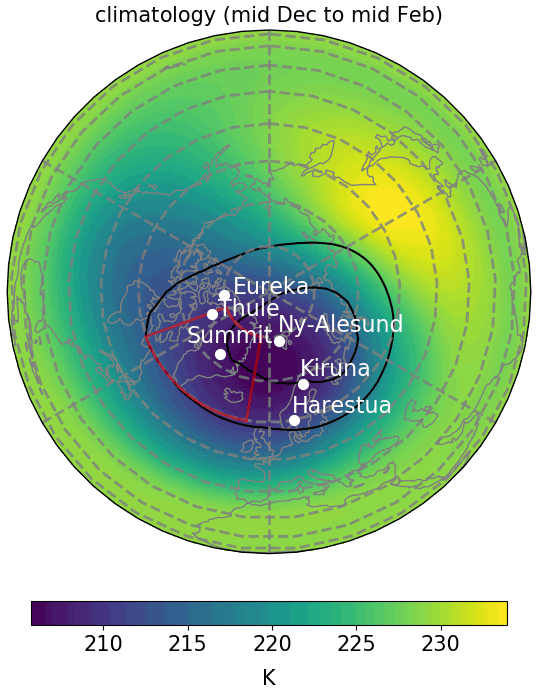
Figure 1The climatology of temperature at 10 hPa and EPV at the potential temperature of 850 K during wintertime (DJF) over the Northern Hemisphere. The climatology is based on non-SSW years from 2004 to 2019. The map coloring shows the average winter temperature. The black contour lines are 600 and 800 EPV units (10−6 K m2 kg−1 s−1). The locations of the observational sites are shown by white dots. Greenland sector is shown by the red polygon.
In Sect. 2, MERRA-2 and other independent observations are described. The methodology of comparisons and the dynamical analysis are presented in Sect. 3. The results of the comparison between MERRA-2 and independent observation are discussed in Sect. 4. The evolution of each SSW and its impact on ozone are discussed in Sect. 5. Discussion of transport mechanisms of ozone is provided in Sect. 6. Section 7 presents the conclusions of this research study.
The Modern-Era Retrospective Analysis for Research and Application, Version 2 (MERRA-2), from NASA's Global Monitoring and Assimilation Office (GMAO) uses the GEOS-5 atmospheric data assimilation system (Molod et al., 2015; Gelaro et al., 2017). A variety of data sets are incorporated into a general circulation model to create 3-dimensional MERRA-2 ozone datasets with a time frequency of 3 h (Wargan et al., 2017; Gelaro et al., 2017). Total column ozone from the Solar Backscatter Ultraviolet Radiometer (SBUV) (1980 to 2004) and the Ozone Monitoring Instrument (OMI) (since 2004) and retrieved ozone profiles from SBUV (1980 to 2004) and the MLS (since August 2004, down to 177 hPa to 2015, down to 215 hPa after 2015) are used to estimate ozone in MERRA-2 (Gelaro et al., 2017).
MERRA-2 data are available online through the NASA Goddard Earth Sciences Data Information Services Center (GES DISC; https://disc.gsfc.nasa.gov/, last access: 18 April 2022). MERRA-2 has been used to study ozone trends and processes (Coy et al., 2016; Knowland et al., 2017; Wargan et al., 2018; Albers et al., 2018; Shangguan et al., 2019). In this study, the ozone dataset from the MERRA-2 reanalyses at a spatial resolution of will be used. To have the finest possible vertical resolution for the comparisons with observations, MERRA-2 ozone at the model levels is used (GMAO, 2015a). Other dynamical variables such as temperature, and the northward and vertical wind velocities (v, ω), are extracted from the pressure-level MERRA-2 dataset (GMAO, 2015b), which facilitates the calculation of variables such as EPV and potential temperature (θ).
In reanalysis products such as MERRA-2, methods of analysis, model uncertainties, and observations cause uncertainties in the products (Rienecker et al., 2011). MERRA-2 is shown to have the best agreement with stratospheric ozone observations compared to other reanalysis data (Davis et al., 2017). Previously, MERRA-2 ozone data were validated using ozonesondes and satellite data from 2005 to 2012 (Gelaro et al., 2017; Wargan et al., 2017). MERRA-2 agreement with independent observations has been improved since 2005 by assimilating OMI and MLS. Comparison with independent satellite observations shows an average standard deviation of the differences of 5 % and 11 % in the upper and lower stratosphere, respectively (Wargan et al., 2017). The average standard deviation of 20 % has been reported for the comparison between MERRA-2 lower stratospheric ozone and ozonesondes (Wargan et al., 2017). However, uncertainties are expected to be magnified at high latitudes because of higher dynamical variability (Wargan et al., 2017). Moreover, the anomalous atmospheric dynamics, displaced/split polar vortex, and hemispherically asymmetric conditions during SSWs may cause complexity and additional uncertainties in estimation of ozone flux/transport terms. Thus, it is important to investigate the quality of MERRA-2 ozone simulations during highly altered circulations such as SSWs. This study provides a comprehensive comparison using ground-based remote sensing and in situ observations to MERRA-2 ozone datasets over northern high latitudes during SSWs.
We use a uniquely dense network of observations in the high latitudes to study a region of the Arctic that is climatologically important in terms of stratospheric circulation (Fig. 1). Ozonesondes have been used to monitor ozone for decades as the most direct measurement of the vertical ozone profile (Tiao et al., 1986; Logan, 1994; Logan et al., 1999; Stolarski, 2001; Gaudel et al., 2015; Bahramvash-Shams et al., 2019). Ozonesonde profiles provide a good standard for validation because they have high accuracy, fine vertical resolution of less than 100 m, year-round launches, and low sensitivity to clouds (McDonald et al., 1999; Ancellet et al., 2016; Sterling et al., 2018).
In this study, ozonesonde measurements at Eureka, Ny-Ålesund, Thule, and Summit will be used to investigate the uncertainties of MERRA-2. The locations of each station and the length of the ozonesonde measurements at each site are shown in Fig. 1 and Table 1. Most of the ozonesonde measurements can be found at the World Ozone and Ultraviolet Radiation Data Centre (WOUDC), while ozonesonde data in the United States are obtained from NOAA's Earth System Research Laboratory, including data from Summit Station, Greenland. The detailed description and uncertainty estimation of ozonesonde measurements have been discussed in previous studies (Komhyr, 1986; Johnson et al., 2002; Smit et al., 2007; Tarasick et al., 2016; Sterling et al., 2018).
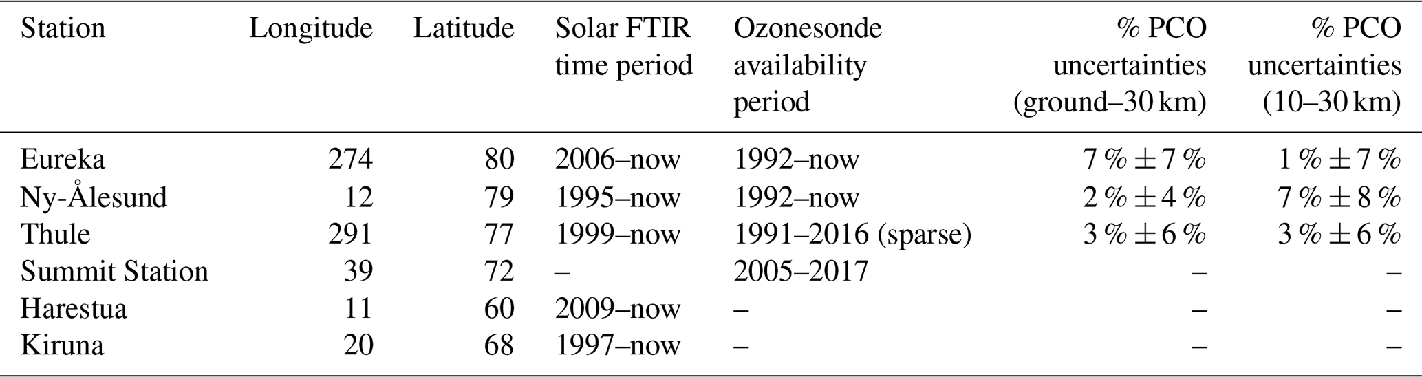
Table 1Site locations for NDACC FTIRs and ozonesondes. Uncertainties of FTIRs at three sites with ozonesondes are given by averaged subtraction and standard deviation of ozonesondes from the retrieved ozone from FTIR, as uncertainty of partial column ozone (PCO) in both ground to 30 km and 10 to 30 km.
In addition to ozonesondes, ground-based remote sensing data are also used in this paper to study the uncertainties in the MERRA-2 dataset. Retrieved ozone from ground-based Fourier transform infrared (FTIR) interferometers has been used for long-term ozone analysis (Vigouroux et al., 2008; García et al., 2012; Vigouroux et al., 2015). In this study, ozone profiles retrieved from FTIR at five high-latitude sites (Eureka, Ny-Ålesund, Thule, Harestua, and Kiruna) were obtained from NDACC (Network for the Detection of Atmospheric Composition Change) and used to validate MERRA-2. The location of each site is shown in Fig. 1 and Table 1. These datasets are available at http://www.ndacc.org (last access: 10 March 2021).
The NDACC FTIR instruments measure solar radiation in a wide spectral bandwidth of 600–4500 cm−1 at a high spectral resolution of 0.0035 cm−1. The retrieval of ozone profiles from NDACC FTIR instruments uses the optimal estimation method (Rodgers, 2000). NDACC retrievals use the spectroscopic database from HITRAN 2008 (Rothman et al., 2009). To retrieve trace gas information from the measured spectra using optimal estimation, additional information is required to constrain the result and find the optimal answer. Meteorological parameters from the National Centers for Environmental Prediction (NCEP) and monthly trace gas profiles from the WACCM4 (Marsh et al., 2013) are used as prior conditions. More details of the NDACC ozone retrieval steps, configuration, and instrument specifications are discussed by Vigouroux et al. (2008, 2015). These instruments require sunlight and clear-sky conditions, which restricts observations to the polar day at high latitudes.
The retrieved total ozone column and the stratospheric partial columns from FTIR are expected to have uncertainties of 2 % and 6 %, respectively (Vigouroux et al., 2015). This study updates the uncertainties found by previous studies by adding additional years of data and by focusing on three high-latitude sites that contain both ozonesondes and FTIR measurements. The FTIR ozone retrievals showed a high correlation (∼90 %) in comparison to ozonesonde profiles measured at Eureka, Ny-Ålesund, and Thule, with uncertainties shown in Table 1. Overall, the uncertainties are slightly higher than the averaged uncertainties reported by Vigouroux et al. (2015). This is more pronounced at Eureka due to the high solar zenith angle and the possibility that, at times, the FTIR views a slant path through the atmosphere that extends through the edge of the polar vortex. More details on the ozone retrievals at Eureka can be found in Bognar et al. (2019). As shown in Table 1, the NDACC retrievals are biased high when compared to the ozonesondes. Also, the bias is higher at Eureka (7 %) than at either Ny-Ålesund (1 %) and Thule (3 %). These biases and standard deviations (shown in Table 1) are less than the differences between MERRA-2 and the ozonesondes (20 %) discussed above, indicating that the NDACC FTIR ozone retrievals can be used to increase the robustness of the uncertainty analysis of the MERRA-2 ozone dataset.
In this section, the details of the different methods used in this study are discussed, including the comparison methodology, detection of SSWs, and the derivation of dynamical parameters used to investigate ozone transport.
To have comparable points, NDACC and in situ site locations, shown in Fig. 1 and Table 1, are extracted from the nearest grid MERRA-2 ozone dataset. The nearest instantaneous 3-hourly MERRA-2 ozone dataset is compared to the associated ozonesonde profile and the FTIR-retrieved ozone. The MERRA-2 ozone data are compared to ozonesondes at the model levels, up to the maximum measured altitude. Since the vertical resolution of the FTIR retrieval does not match the vertical resolution of the assimilation system, a more direct comparison involves a convolution of the reanalysis profiles using the FTIR averaging kernel (Rodgers and Connor, 2003). Averaging kernels characterize the vertical resolution and sensitivity of FTIR instruments to the atmospheric ozone variability at various altitudes (Rodgers, 2000). Equation (1) shows how the averaging kernel is applied with the reanalysis data to account for the sensitivity of retrievals (Rodgers and Connor, 2003), producing a smoothed ozone profile.
where xs is the final smoothed profile, xh is the reanalysis estimated profile, and xa and A are the a priori and averaging kernel of ozone mixing ratio for the retrieval respectively. The smoothing method effectively applies the sensitivity of the retrieval to the ozone mixing ratio profile from the reanalysis using the averaging kernel and the priori information to create comparable profiles. (Rodgers and Connor, 2003). MERRA-2 data are interpolated to the vertical grid of the retrievals before Eq. (1) is applied.
The high spectral resolution of the solar FTIR measurements makes it possible to retrieve partial ozone columns in addition to the total column ozone. Based on the mean average kernels at all five stations, four partial column ozone (PCO) are determined in this study over the following altitude regions: ground–8, 8–15, 15–22, and 22–34 km. The PCO amounts are also used to analyze uncertainties in the MERRA-2 ozone dataset. The comparison results are discussed in Sect. 4.
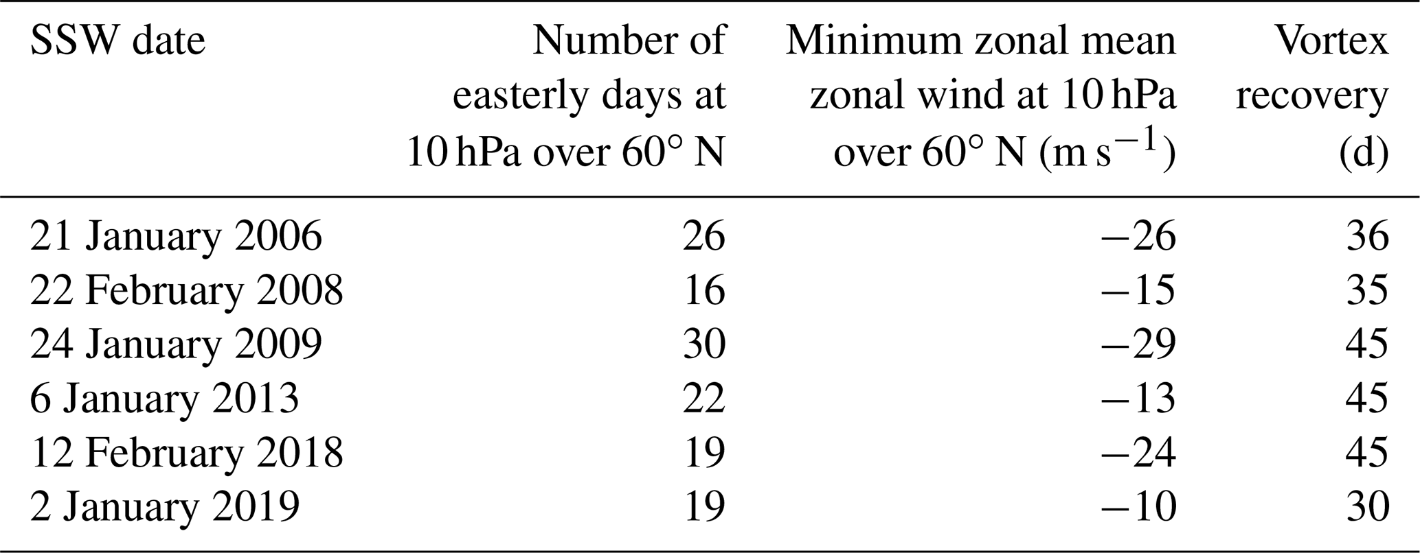
There are a variety of definitions for detecting major SSWs (Charlton and Polvani, 2007; Butler et al., 2015; Palmeiro et al., 2015). This study uses wintertime reversals of the daily-mean, zonal mean zonal winds at 60∘ N and 10 hPa from the MERRA-2 dataset (Butler et al., 2017). The dates of major SSWs since August 2004 (MLS data incorporation into MERRA-2) are calculated using MERRA-2 data following the method described by Charlton and Polvani (2007). This paper focuses on six persistent mid-winter (December-February) major warmings in this period that exhibited persistent easterly zonal mean zonal winds with a duration of at least 16 d (Table 2). Table 2 includes the duration, magnitude of the easterly zonal wind, and the duration of polar vortex recovery for each SSW; all information is derived from MERRA-2 data. It should be noted that the duration of the easterly wind shown in Table 2 is not necessarily consecutive. Two major SSWs during the 2004–2020 time period are not included in the main results of our study because they did not meet the persistence criteria. The major SSW in 2007 exhibits only 4 d of easterly zonal mean zonal winds, while the major SSW in February 2010 exhibits only 9 d. However, SSWs in 2007 and 2010 are included in the regression analysis for Fig. 6 for more robust statistics, which also shows that they had some of the lowest impact on ozone.
Table 2SSW dates, duration, magnitude, and the duration of polar vortex from 2004 to 2020. The number of easterly days at 10 hPa over 60∘ N is shown as the duration SSW. The magnitude of SSWs is defined by the minimum zonal mean zonal wind at 10 hPa over 60∘ N during each SSW. The total number of easterly days associated with the event is not necessarily consecutive. The duration of polar vortex recovery is defined as the number of days that the zonal averaged EPV takes to reach the climatological zonal EPV.
This study also analyzes the impact of different dynamical transport mechanisms on ozone for each of the major SSWs. The zonal mean tracer concentration is a balance between transport processes and the chemical sources and sinks, as shown in the continuity equation of the transformed Eulerian mean (TEM) (Andrews et al., 1987):
where is the tracer tendency (in this case, ozone mixing ratio tendency), (, ) denotes horizontal and vertical components of the residual circulation, in log-pressure height using a scale height H of 7 km, M is the eddy transport vector, and P and L are chemical production and loss. The overbars stand for the zonal average. Subscript symbols denote partial derivatives (with respect to time (t) and height (z)). The first two terms on the right-hand side of Eq. (2) represent the contribution of advective transport on ozone changes. The vertical component of residual circulation is the dominant contributor of advection () and can be estimated using TEM (Andrews et al., 1987):
where v and w are the meridional and vertical winds, θ is potential temperature, a is the earth radius, φ is the latitude. The prime denotes the departure from the zonal mean. The third term on the right side of Eq. (2) shows the impact of eddy mixing on ozone transport. M can be decomposed into vertical and meridional components M(z) and M(y) respectively: (Andrews et al., 1987):
The contribution of dynamical and chemical drivers of ozone anomalies varies throughout the year. During springtime, both dynamical resupply and chemical depletion strongly modulate ozone changes. Assuming an isolated polar vortex and neglecting isentropic mixing, a previous study showed a similar magnitude of influence from chemical ozone depletion processes and dynamical ozone supply during the springtime (Tegtmeier et al., 2008). However, Strahan et al. (2016) used a chemistry and transport model to show that dynamical processing affects ozone changes by a factor of 2 more than chemical processing during March. However, chemical processes are not significant drivers of ozone changes in the middle stratosphere from November to February in the Arctic because of the polar night (de la Cámara et al., 2018b). Moreover, it has been shown that during years with SSWs, Arctic ozone depletion is significantly diminished (Strahan et al., 2016). However, if prior to or during the SSWs, the polar vortex moves outside of the region of the polar night (to lower latitudes), ozone depletion will occur as shown in the 2013 SSW by Manney et al. (2015). By limiting our analysis to latitudes between 60 to 80∘ N, this impact is minimized in our analysis. Because the impact of the chemical components on the evolution of ozone during SSWs is a less important factor below 30 km (de la Cámara et al., 2018b), the dynamical analysis in this study will focus on altitudes below 30 km. Thus, neglecting P and L below 30 km in further analysis, as chemical production and loss is not an output of reanalysis data, does not lead to significant non-closure in the presented analysis and does not impact our conclusions. In further sections, analysis will focus on middle stratospheric layers between 15 and 30 km.
In this section, the results of the comparisons between MERRA-2 and observations from ozonesondes and FTIR retrievals during SSWs are discussed. Ground-based observations provide an excellent baseline to assess climate models and assimilated systems. However, the use of ground-based observations to directly study the impact of SSWs is challenging because of the coarse time resolution of ozonesondes, limited clear-sky conditions and sunlight for FTIR measurements, and dealing with one profile per site/launch time for each sensor, and its subjectivity to the site location and time. In this study, we take advantage of a dense network of observations over the Greenland sector (60 to 80∘ N and 10 to 70∘ W) to assess the performance of MERRA-2 over the high latitudes. The use of MERRA-2 allows us to investigate the fluctuations over the entire Arctic with consistent temporal and spatial resolution. To visualize the observation frequency and the overall performance of MERRA-2, the time series of PCO from MERRA-2 3-hourly data and ozonesondes and FTIR from winter 2007 to spring 2009 are shown in Fig. 2.
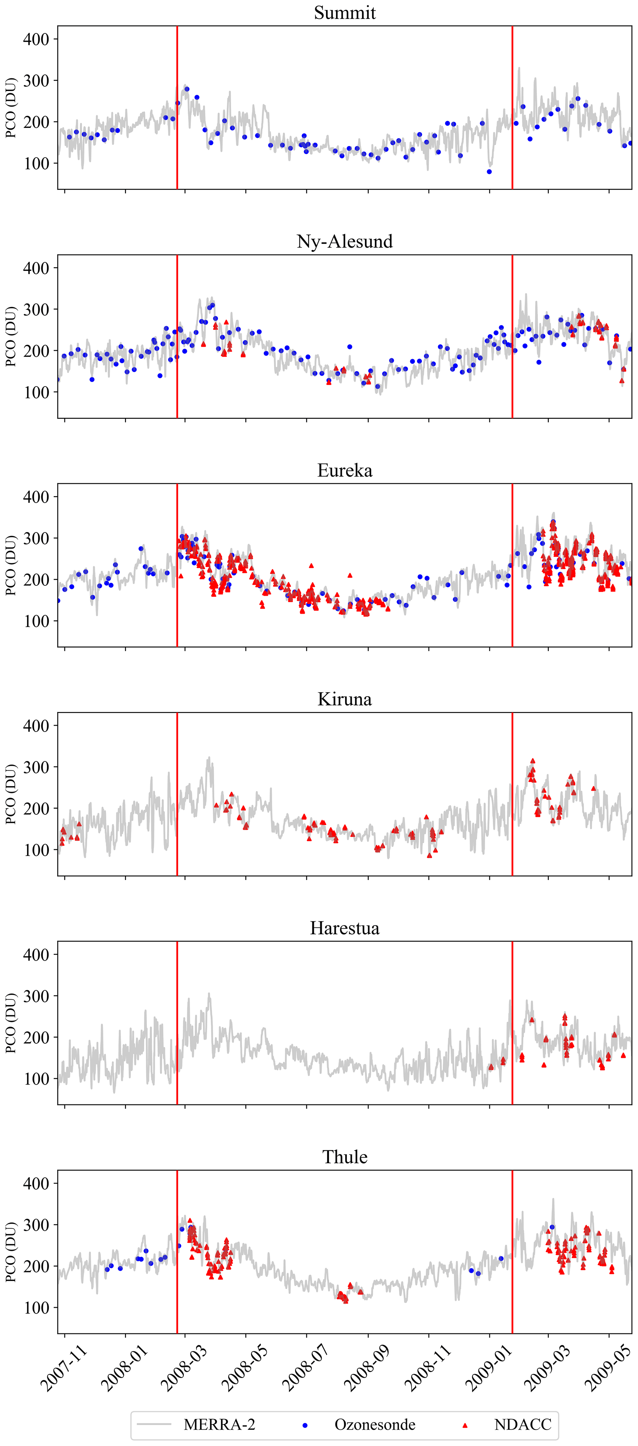
Figure 2Time series of 3-hourly partial column ozone (PCO) of ground to 20 km derived from MERRA-2, solar FTIR, and ozonesondes at the study sites from winter 2007 to spring 2009. MERRA-2 is shown by the gray line. NDACC FTIR data and ozonesondes are shown by red triangles and blue circles, respectively. The vertical red lines highlight the dates of the 2008 and 2009 SSWs.
Two major SSWs occurred during this time period. To exhibit a consistent time series and to avoid the impact of the variability of maximum height of the ozonesondes, PCO from the ground to 20 km is shown. Figure 2 shows the high temporal frequency of the FTIR retrievals compared to ozonesondes during polar day, the consistent frequency of ozonesondes throughout the year, and the gap in solar FTIR retrievals at high latitudes during polar night. The results indicate a good overall agreement of MERRA-2 with observations. The sparsity of FTIR ozone retrievals at Thule in 2008 was due to instrument issues. To have a more clear understanding of the uncertainties in MERRA-2 estimations, more quantitative comparisons are needed.
To investigate the uncertainties of MERRA-2 ozone data during the highly anomalous conditions during SSWs and to consider the enduring impact of SSWs on trace gases, comparisons are performed from 1 December to 1 May for all six events. The results and statistics of comparisons between ozonesondes and MERRA-2 are depicted as the relative differences in Fig. 3. The PCO relative difference is estimated as PCO from MERRA-2 minus ozonesonde PCO divided by ozonesonde PCO for ground to 5 km (G–5 km), 5–10, and 10–30 km. These layers indicate different performances of MERRA-2 by height and show the effect of atmospheric pressure on the contribution of each level to the total ozone column. The G–5 km layer includes the troposphere, and the 5–10 km layer includes the upper troposphere–low stratosphere (UTLS), while the 10–30 km layer includes the lower and middle stratosphere. The partial column is calculated only up to the altitude of the balloon burst of the ozonesonde, if the burst height is below 30 km.
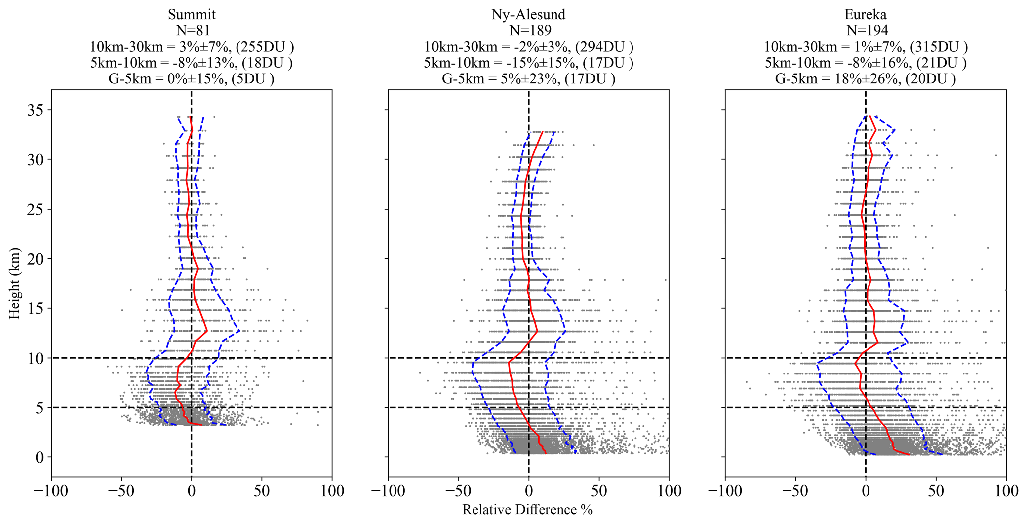
Figure 3Relative differences of ozonesonde and MERRA-2 at each layer at three sites from 1 December to 1 May for 6 years of SSWs. The relative difference is the subtraction of ozonesonde from MERRA-2 ozone dataset divided by ozonesonde for each layer. The normalized mean bias is shown by the red line. The standard deviation of the relative differences from the normalized mean biases are shown by the blue lines. The number of coincident ozonesonde and MERRA-2 comparisons between 1 December and 1 May for the 6 years of SSWs (N) is shown under each site name. The mean and standard deviation of PCO relative differences for three layers (10–30, 5–10, ground–5 km) are summarized for each site. The average PCO value for each layer is shown in parentheses.
Large relative differences between MERRA-2 and the ozonesondes near the surface indicate a well-defined high bias in MERRA-2 at Ny-Ålesund and Eureka. The occasional extreme low ozone mixing ratios observed in the lower atmosphere and near the surface are linked to catalytic reactions involving bromine. This chemical ozone depletion is more common at Arctic sites near the ocean (Tarasick and Bottenheim, 2002). The extreme low ozone values near the surface are not represented in MERRA-2 as it does not include bromine chemistry.
Overall, the variability of the relative differences at lower altitudes is larger (Fig. 3). Ny-Ålesund and Eureka show 5 % (±23 %) and 18 % (±26 %) mean (± SD) difference ratios at G–5 km. However, the G–5 km layer, on average, contains less than 20 DU, which is less than 6 % of total column ozone (TCO). PCO of the G–5 km layer is only 1.5 % of TCO at Summit Station where the site elevation is 3.2 km. The PCO difference ratio at Summit station shows very small bias, with a standard deviation of ±15 %.
The positive bias decreases higher in the troposphere, and the scatter plot shows negative relative differences. From 5 to 10 km, a negative mean bias exists at all sites; however these biases are accompanied by a larger the standard deviation. The mean PCO relative differences from 5 to 10 km are −8 % (±13 %), −15 % (±15 %), and −8 % (±16 %) at Summit Station, Ny-Ålesund, and Eureka.
The MERRA-2 ozone data between 10 and 30 km are highly correlated with the ozonesondes with R2>90 % (not shown). From 10 to 15 km, the relative differences are slightly positive and, above 15 km, a negligible bias and low standard deviations are observed. The mean PCO difference ratio in the 10–30 km layer is equal to or less than 3 % (±7 %) at all stations. The differences between 10 and 30 km are more impactful in TCO uncertainty analysis because this region contributes most to the total column ozone. (The average PCO for each layer is reported in Fig. 3.)
Figure 4 summarizes the comparison between the MERRA-2 and the FTIR retrievals for 1 December to 1 May for all 6 SSW years. The partial column comparisons for ground to 8, 8–15, 15–22, and 22–34 km are shown. Here the partial columns are defined based on the averaging kernel of the NDACC retrievals. The mean and standard deviation of relative differences and the mean PCO for each layer are shown in Fig. 4.

Figure 4Same as Fig. 3 but for relative differences of FTIR retrieved ozone from MERRA-2. Statistical summaries of the MERRA-2 and NDACC comparisons in four layers (ground to 8, 8–15, 15–22, and 22–30 km) for each station are shown above each plot.
The layers between 15–22 and 22–34 km contain the most column ozone, with averages of 146 and 101 DU, respectively. MERRA-2 and the FTIR retrievals have good agreement in these layers, with relative differences of and , respectively.
In the lowest layer, the differences are the largest, with a standard deviation ratio of higher than 15 % at all stations and mean differences in the range of −7 % to 3 %. Large differences are observed between 8–15 km, where MERRA-2 estimates 7 %–13 % more ozone than the FTIR retrievals, and the standard deviations are large. Large differences and standard deviations below 15 km indicate that higher uncertainties exist in both the FTIR retrievals and the MERRA-2 estimation
In conclusion, when compared to observations, MERRA-2 captures large fluctuations in middle stratospheric ozone at high northern latitudes during winters and early spring that are impacted by SSWs. The agreement between MERRA-2 ozone with observations during SSWs motivates the use of MERRA-2 dataset to further understand mid-stratospheric ozone fluctuations during SSWs. The differences in the lower stratospheric and tropospheric layers exhibit larger values. The higher uncertainties below 10 km during the 5 months impacted by SSWs are consistent with higher uncertainties in MERRA-2 in these layers year-round, as seen in previous studies (Gelaro et al., 2017; Wargan et al., 2017). However, still large fluctuations of lower atmosphere ozone are discernible from MERRA-2 data (Knowland et al., 2017; Jaegleì et al., 2017; Albers et al., 2018). The maximum height of ozonesondes is around 30–35 km, and ground-based remote sensing loses sensitivity with increasing altitude; thus this study cannot improve previous research on the upper stratosphere where higher uncertainties were reported compared to the mid-stratosphere. Because more than 80 % of ozone molecules exist in the middle stratosphere (15 to 30 km), the total column uncertainty is dominated by uncertainties in mid-stratospheric layers. In the following section, we discuss ozone variability in the total column and the vertical profile up to 60 km, while our primary analysis is focused on ozone and dynamical processes in the mid-stratospheric layers, which contribute most to the TCO and where the measurements are most reliable.
Disturbances in stratospheric circulation have an impact on stratospheric trace gas concentrations. Consequently, the temporal changes of trace gas concentrations can provide a better understanding of atmospheric circulation including vertical and horizontal transport (Manney et al., 2009a). In this section, the impact of altered circulation patterns on ozone is analyzed, and by investigating the evolution of the polar vortex and temperature, more detailed characterization of ozone variability is provided.
To understand the alteration of ozone and the average position of the polar vortex before and after each SSW, the anomaly of total column ozone (TCO) and the average Ertel EPV are investigated. The anomalies of TCO average and EPV average for the 15 d preceding and 15 d after each of the SSWs are shown in Fig. 5. The TCO anomaly is calculated using a climatology based on the same days of averaged non-SSW years since 2004. EPV contours of 600 and 800 (10−6 K m2 kg−1 s−1) at isentropic level with the potential temperature of 850 K (∼30 km) indicate the dominant area of the polar vortex. In the following section the main characterization of each SSW, the evolution of the polar vortex, and TCO changes are discussed.
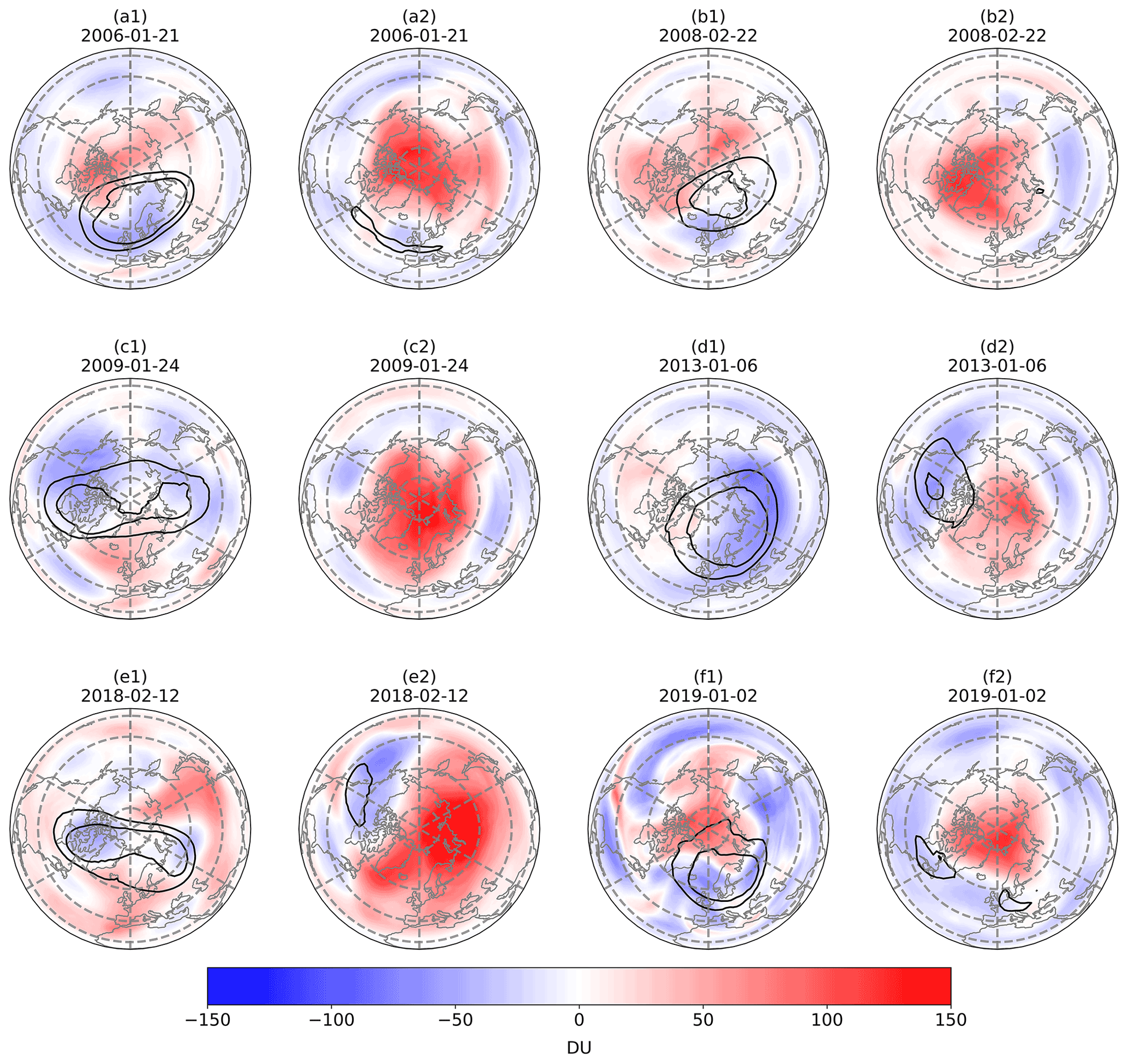
Figure 5The anomaly TCO average over 15 d prior (alphabet1, first and third columns) and 15 d after each SSW (alphabet2, second and fourth columns) compared to climatology on non-SSW years. EPV at the potential temperature of 850 K is averaged for the same period similar to TCO. Contour lines show the EPV map at 600 and 800 10−6 K m2 kg−1 s−1.
-
2006. On 21 January 2006, the second strongest and prolonged major SSW since 2004 was detected (Table 2, Siskind et al., 2007; Manney et al., 2008b; 2009a). The easterly zonal mean zonal wind lasted 26 d. Prior to the major SSW, a minor SSW was detected on 9 January (Manney, 2008b, 2009a). The polar vortex moved toward Siberia and receded away from Greenland during the minor warming. The polar vortex was then displaced westward and equatorward toward northwestern Europe before the major SSW, as shown in Fig. 5a1.
-
2008. The dynamical circulation was quite variable during winter 2008. Two minor SSWs in mid-January and late January and one major SSW in late-February are recorded in 2008 (Goncharenko and Zhang, 2008; Flury et al., 2009; Thurairajah et al., 2010; Korenkov et al., 2012). The easterly winds lasted 16 d after the major warming on 22 February. This event is recorded as the latest in the winter season and the least prolonged among the six SSWs considered in this study (Table 2). The polar vortex is displaced mostly over northwest Europe during the development of the SSW in 2008 as shown in Fig. 5b1. The polar vortex displacement over Europe led to ozone depletion and the enhancement of stratospheric water vapor over northern Europe by mid-February (Flury et al., 2009).
-
2009. Following an undisturbed and cold early winter, the strongest and most persistent SSW among this study's events occurred on 2 January 2009 as shown in Table 2 (Manney et al., 2009b; Harada et al., 2010; Lee and Butler, 2020). The extended elongated shape of the polar vortex before the SSW can be seen in Fig. 5c1, which was followed by a split vortex. The prolonged SSW in late January recorded 30 d of easterlies at 10 hPa, with a maximum magnitude of 29 m s−1 (Table 2).
-
2013. The atmospheric disruption associated with the major SSW on 6 January 2013 displaced the polar vortex toward Europe (Fig. 5d1) and eventually split the stratospheric polar vortex into smaller vortices over Canada and Siberia in mid-January to late January (Manney et al., 2015). The isolated, offspring vortex over Canada lasted for more than 2 weeks, as shown in Fig. 5d2.
-
2018. A major SSW was detected on 12 February 2018. However, the disturbed circulation started in January, with 8 d of zonal wind deceleration occurring in mid-January (Rao et al., 2018). The elongated pattern of EPV from Europe to eastern Canada shown in Fig. 5e1 indicates a highly disturbed vortex prior to the major SSW, resulting in a vortex split (Karpechko et al., 2018; Rao et al., 2018; Butler et al., 2020). The split vortices were located over Canada/northwest United States and northwestern Europe and lasted for almost a week after the detected SSW. The signal of the offspring vortex after the SSW event over Canada is visible in Fig. 5e2. The major SSW caused record-breaking cold surface temperatures in northwest Europe (Greening and Hodgson, 2019).
-
2019. The major SSW on 2 January 2019 (Butler et al., 2020; Rao et al., 2019; Schranz et al., 2020) is the earliest in the winter season and weakest in magnitude of reversal among the most recent six events studied here (Table 2). The polar vortex was displaced towards Europe before the major SSW occurred (Fig. 5f1). The continuous wave activity caused a vortex displacement to be followed by a split vortex. The resulting vortices were located over the northeastern United States and northwestern Europe as shown in Fig. 5f2.
As shown in Fig. 5, the averaged vortex displacement occurs towards the southeast (Europe) prior to the major SSW as seen in 2006, 2008, 2013, and 2019 (hereafter the displaced vortex SSWs) and is accompanied by an early positive ozone anomaly in the region outside of the vortex, which includes parts or all of the North Pole, high-latitude North America, eastern Siberia, and the Greenland sector. After the vortex breakdown, the geographical extent of the positive ozone anomalies is mostly limited to high latitudes, with a fairly symmetrical shape around the Arctic in these cases. On the other hand, an elongated averaged polar vortex prior to the major SSW as seen in 2009 and 2018 (hereafter the elongated vortex SSWs) is associated with negative ozone anomalies over a large extent of high latitudes, followed by strongly positive TCO anomalies over an extensive area after vortex breakdown.
The averaged polar vortex state we refer to in this study is different, though often related to, split and displaced vortex morphology discussed in previous literature (e.g., Charlton and Polvani, 2007). As seen during the SSWs in 2018 and 2009, in which the polar vortex split, the 15 d average polar vortex before those events is elongated. Other events, such as those in 2013 and 2019, are first displaced and then split. However, here we consider them displaced SSWs if the 15 d average EPV prior to the event is displaced and not elongated. Previous studies focused on the connection of the type of polar vortex breakdown to its impact on the speed of trace gas transitions (Charlton and Polvani, 2007; Manney et al., 2009b). This study investigates the modulation of the magnitude and extent of ozone changes, and the results show that the average EPV shape before the vortex breakdown is more influential than the final form of polar vortex breakdown.
To investigate the connection of polar vortex strength and TCO, the scatter plot of the zonally averaged (60 to 80∘ N) EPV change at the potential temperature of 850 K versus the corresponding change in TCO (60 to 80∘ N) is shown in Fig. 6. All averages are area-weighted, and the ratio of change for each variable is estimated as the average of 15 d after SSWs subtracted by the average of 15 d before the SSWs and divided by the average of 15 d before the SSWs. To increase the robustness of regression analysis, SSWs in 2007 and 2010 are also included here (Fig. 6). The correlation between the magnitude of change in EPV and TCO is very strong (R2=90 %). The elongated vortex SSWs (2009 and 2018) exhibit a higher magnitude of change in both EPV and TCO in this period. This result shows that the averaged polar vortex shape before the SSWs is connected to the EPV change and then dramatically influences the magnitude of ozone changes at high latitudes.
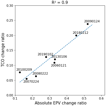
Figure 6The zonally averaged EPV change ratio at the potential temperature of 850 K against the corresponding change in TCO for six studied SSW as well as less persistent major SSWs in 2007 and 2010. The ratio of change for each variable is estimated as the average of 15 d after SSWs subtracted by the average of 15 d before the SSWs and divided by the average of 15 d before.
As the Greenland sector is one of the critical regions that is climatologically isolated by the polar vortex, the variability of area-weighted ozone average over the Greenland sector (60 to 80∘ N and 10 to 70∘ W) as well as the zonal average (60 to 80∘ N) is analyzed to investigate the similarities and differences of the impacts of SSWs on zonal and regional high-latitude ozone. The structure of ozone anomalies in the zonal minus Greenland sector is similar to the zonal average. The Greenland sector has been shown to be uniquely sensitive to dynamical forcing associated with the Quasi-Biennial Oscillation (QBO) (Anstey and Shepherd, 2014; Bahramvash-Shams et al., 2019). Moreover, the air masses above the Greenland sector are more strongly isolated than at other Arctic longitudes during wintertime, as shown by the climatology of the polar vortex and its associated minimum temperature in Fig. 1. Thus, it is important to understand the regional impact of SSWs on the Greenland sector.
To track the strength of the polar vortex, the area-weighted average of EPV at the potential temperature of 850 K over the zonal average (60–80∘ N) and the Greenland sector (60–80∘ N, 10–70∘ W) from 40 d before to 60 d after each SSW is shown in the first column of Fig. 7. The evolution of the area-weighted average of TCO for the zonal average and the Greenland sector is shown in the second column of Fig. 7. The climatologies of EPV and TCO for both the zonal average and Greenland sectors in Fig. 7 are estimated based on non-SSW years between 2004 and 2019. To quantify the influence of SSWs on ozone, the average TCO for the period spanning 40 d before to 60 d after the SSWs is shown in the bottom right of each plot, as well as the ratio of the changes.

Figure 7EPV at the potential temperature of 850 k (first column) and TCO (second column) over the Arctic zonal mean 60–80∘ N (orange line) and Greenland sector (blue line) during the 40 d before and 60 d after each SSW (each row). Climatology of EPV and TCO for the zonal and Greenland sector is shown by dashed orange and blue lines, respectively. The average total column ozone (TCO) during the 40 d before and 60 d after and the percentage of change for each SSW are shown in the bottom corner of the second column.
The Greenland Sector is located inside the climatological polar vortex area (Fig. 1), which explains the higher intensity of climatological EPV over the Greenland sector compared to the zonal climatology in Fig. 7. The impact of minor SSWs in 2006 (around lag −25 and −19) and in 2008 (lag −30 and −15), as well as sudden polar vortex displacement to Eurasia in 2019 (lag −20), showed a stronger signal on the averaged EPV over the Greenland sector, with a larger drop in EPV in this region compared to the zonal mean. The duration of the polar vortex recovery is defined by the number of days between the date of the SSW and the date in which the zonal EPV returns to its climatological value, as reported in the last column of Table 2. The fastest recovery of 30 d is observed in 2019 (also the least minimum easterly value of the study's SSWs), and the longest recovery duration of around 45 d is observed in 2009, 2013, and 2018. The recovery duration is similar with only a few days' difference if the EPV over the Greenland sector is used instead.
Compared to the 40 d average of TCO prior to the SSW, the highest percent zonal TCO increase of 29 % is observed for one of the elongated polar vortex SSWs in 2009. The relative increase in TCO over the Greenland sector (blue line) is higher compared to the zonal average (orange line). The Greenland sector is climatologically inside the polar vortex area and has a lower TCO value during strong polar vortex, which consequently exhibits higher relative increase after the vortex breakdown and mixing. However, dynamically disturbed winters such as years with minor SSWs before the major SSWs hinder the higher relative TCO increase over the Greenland sector compared to the zonal average. For instance, in 2006, the polar vortex weakened around 25 d before the major SSW (first column of Fig. 7, TCO, 2006) due to a minor SSW, which coincides with the averaged TCO (solid line) increase compared to the climatology (dashed line), as seen in the second column of Fig. 7 (TCO, 2006). The earlier timing of the positive anomaly caused a lower value in the TCO change after the event. The relative TCO increase over the Greenland sector exhibits a higher value during elongated polar vortex SSWs, with 37 % in 2018 and 31 % in 2009. More details of physical mechanisms that cause variability in ozone during SSWs are discussed in Sect. 6.
Analyzing the vertical structure of ozone provides more details of the impact of SSWs. Figure 8 shows the temporal evolution of the vertical structure of ozone as a cross-section of area-weighted ozone anomalies for both the zonal average (60 to 80∘ N) and the Greenland sector from 40 d before to 60 d after each SSW. The anomalies are estimated with respect to the climatology of non-SSW years between 2004 and 2019. The positive ozone anomaly in mid-stratospheric layers (15 to 30 km) starts a few weeks (15 to 25 d) prior to the displaced vortex SSWs (2006, 2008, 2013, and 2019) over both the zonal average and the Greenland sector. The negative ozone anomalies 15 d before the SSWs and extreme positive ozone after the SSWs in mid-stratospheric layers for the two elongated vortex SSWs (2009, 2018) are evident. The enduring impact of SSWs on ozone in different atmospheric layers is clear in all cases and shows a similar pattern for both the zonal averaged and the Greenland sector. As expected, the structures of ozone anomalies are smoother in the zonal average compared to the Greenland sector. The impact on ozone with the shortest duration occurred in 2008, which has multiple disturbances in the circulation and the shortest duration of easterlies (Table 2).
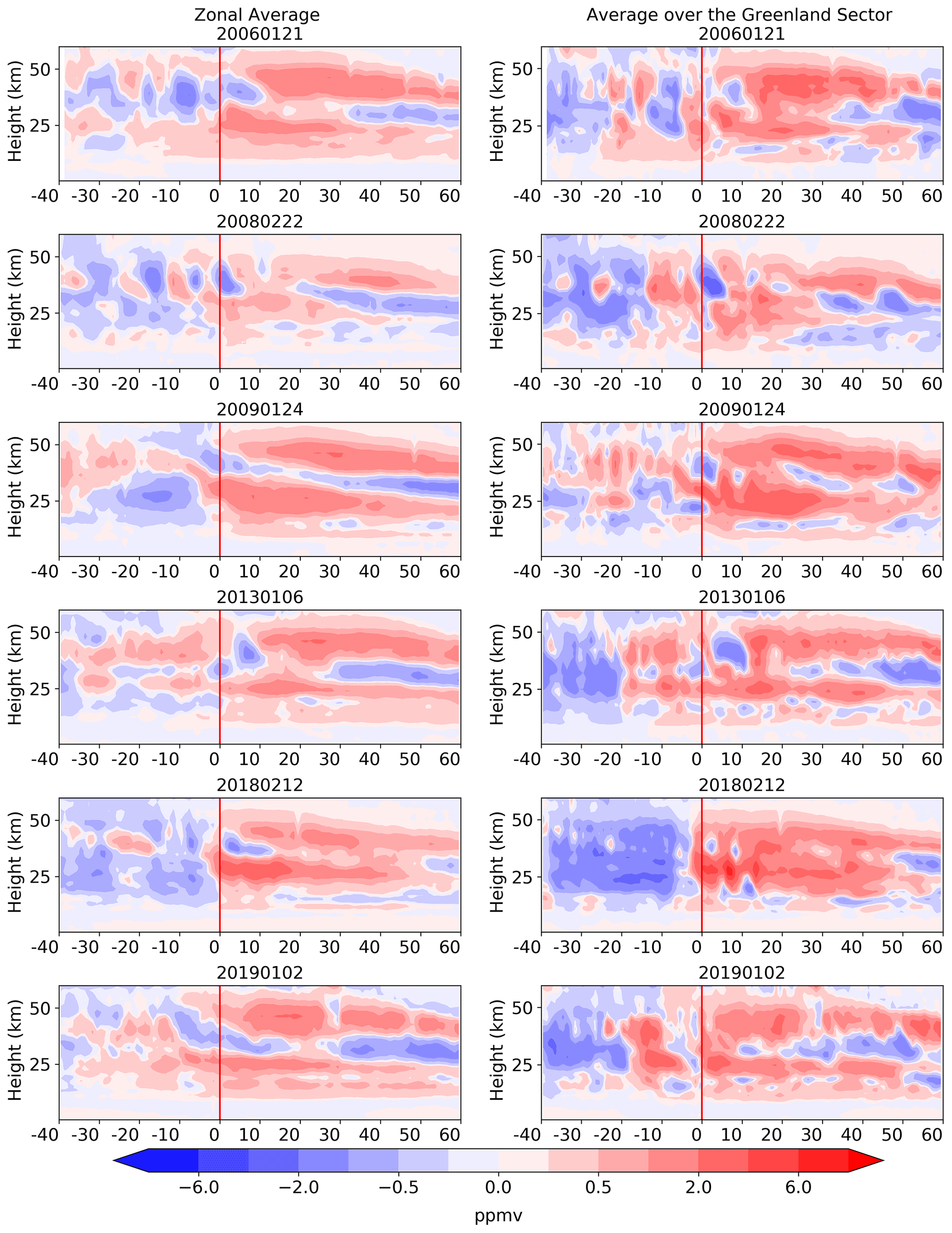
Figure 8The cross-section of ozone anomaly during the 40 d before to 60 d of each SSW averaged over the latitude band 60–80∘ N and Greenland sector (60–80∘ N, 10–70∘ W). The vertical red line shows the SSWs' incident date. Climatology was created using non-SSW years since 2004. The vertical coordinate is the log-pressure height.
To highlight the temperature variation, Fig. 9 shows the cross-section of the temperature anomaly for the zonal average from 40 d before to 60 d after each SSW. Figure 9 focuses only on the zonal average, as the anomaly of temperature profile had similar patterns over the zonal and the Greenland sectors. The positive temperature anomalies in mid-stratospheric layers start a few weeks before the SSWs in the four cases of a displaced vortex (2006, 2008, 2013, and 2019). On the other hand, the intrusion of the positive temperature anomalies to mid-stratospheric layers is almost coincident with SSWs in the two elongated vortex cases. The gradual temperature increases in displaced SSWs point to a buildup of wave forcing in these cases compared to elongated cases. The next section provides more detailed discussion of dynamical mechanisms related to stratospheric ozone changes during SSWs. The duration of positive temperature anomalies in mid-stratospheric layers is 10 to 30 d shorter than ozone positive anomalies (Figs. 8 and 9). The positive temperature anomaly is more persistent at lower levels of the stratosphere, where the enduring impact of SSWs on mid-stratosphere ozone (up to 25–30 km) is clear in all of the SSWs studied here.

The cyclonic polar vortex during wintertime is generated in response to the seasonality of radiative cooling. The intensified wave forcing before the SSW is manifested by both accelerated tropical upwelling and polar downwelling and by poleward transport of low EPV air parcels. The conservation of EPV causes anticyclonic circulation, which gradually drives easterly zonal mean zonal winds and leads to the displacement or splitting of the polar vortex. The resultant reduction in the vorticity induces strong descent and consequently an adiabatic temperature increase in the stratosphere (Matsuno, 1971; Limpasuvan et al., 2012).
Here the MERRA-2 dataset is used to determine the impact of the dynamical terms on ozone changes during each SSW. Because of the constraints in tracer continuity estimation using Eq. (2), these analyses are estimated over the Arctic zonal average only and not the Greenland sector. The vertical component of the residual circulation () as defined in Eq. (3) is an indicator of wave forcing. The cross-section of the vertical component of residual circulation during the 40 d prior to and 60 d after the SSW over the zonal average (60 to 80∘ N) is shown in Fig. 10. More intense downward propagation is shown by darker blue. The increased wave forcing preceding the SSW is evident in Fig. 10 with negative anomalies, which indicate strong downwelling in the zonal average. Occurrences of minor SSWs can be seen through the early appearance of increased wave forcing, as seen in 2006 and 2008. A very intense and abrupt increase in downward propagation was observed in 2009. Disturbed circulations in the middle stratosphere before the SSWs are seen in 2018 and 2019 (lag −30 to −20 d).
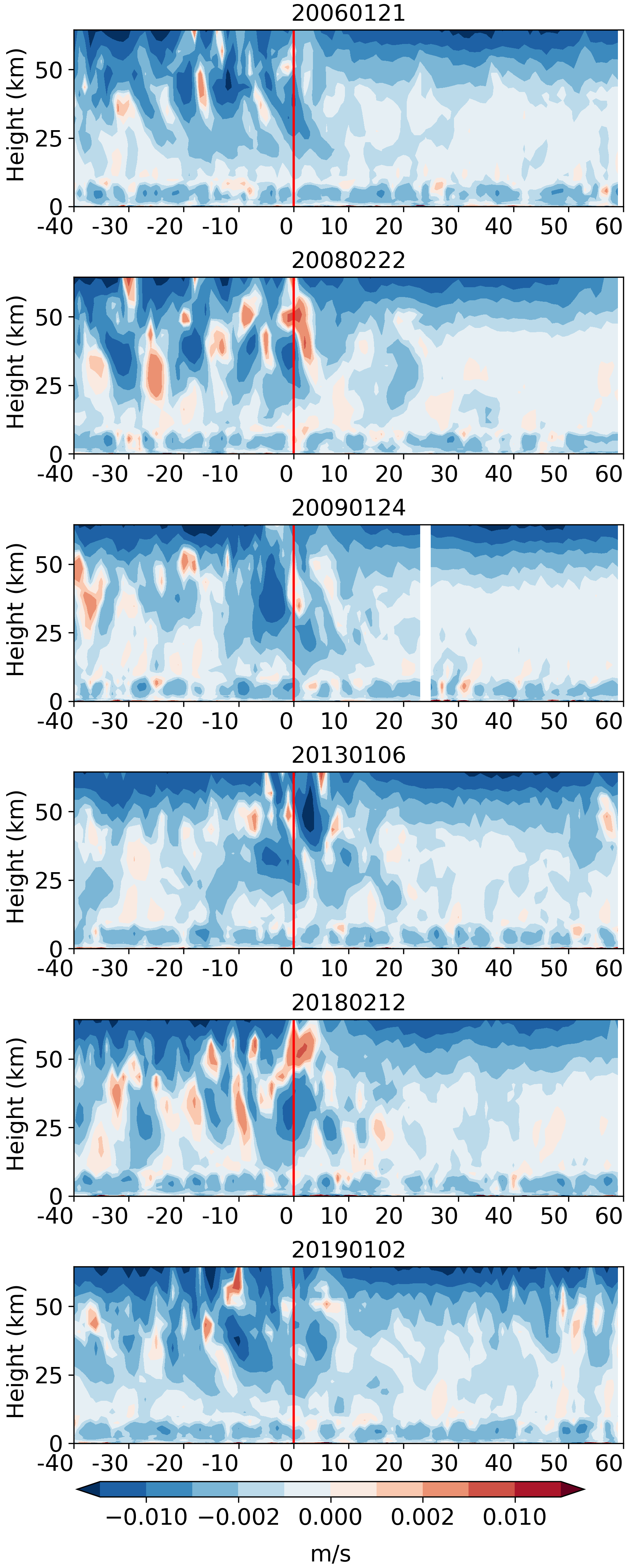
Figure 10Similar to Fig. 8 but for the of the vertical component of the residual circulation, , for zonal average.
Following the SSW, residual circulation is weakened, as shown in Fig. 10. The intensity of increased wave activity is reduced shortly after the SSW. However, the decrease in wave activity is gradual, in general, and lasts a few weeks as shown in Fig. 10. The suppressed wave activity allows for the recovery of the zonal mean zonal wind, temperature, and ozone. Shortly after the SSW, the recovery starts in the upper stratosphere as shown in Fig. 9. However, different radiative relaxation timescales cause a slower recovery in the lower stratosphere compared to upper stratospheric layers (Dickinson, 1973; Randel et al., 2002; Hitchcock and Simpson, 2014). The dynamical alteration suppresses any further upward propagation of the planetary waves, which explains the descending pattern of temperature up to weeks after the SSW (Matsuno, 1971).
The impact of each term in tracer continuity (Eq. 2) on ozone for each SSW is investigated and shown in Fig. 11. The composite effect of chemistry during SSWs is important in the upper stratosphere (de la Cámara et al., 2018b). The analysis of dynamical parameters in this study is limited to 30 km to minimize the impact of chemical processes. Considering the larger uncertainties of ozone estimation in MERRA-2 below 15 km, and the possibility of larger uncertainties in dynamic parameter estimations, this study focuses on the impact of dynamical mechanisms on the middle stratospheric (15–30 km) ozone. The cross-section of ozone tendency (dO3 dt, left side of Eq. 2), the horizontal component of eddy mixing (M(y) as defined in Eq. 4), the vertical component of eddy mixing (M(z) as defined in Eq. 5), the horizontal advection transport (the first term on the right side of Eq. 2), vertical advection transport (the second term on the right side of Eq. 2), and summation of right side Eq. (2) (called the estimated ozone tendency) during the 40 d prior to and 60 d after the SSW over the zonal average are shown in Fig. 11.
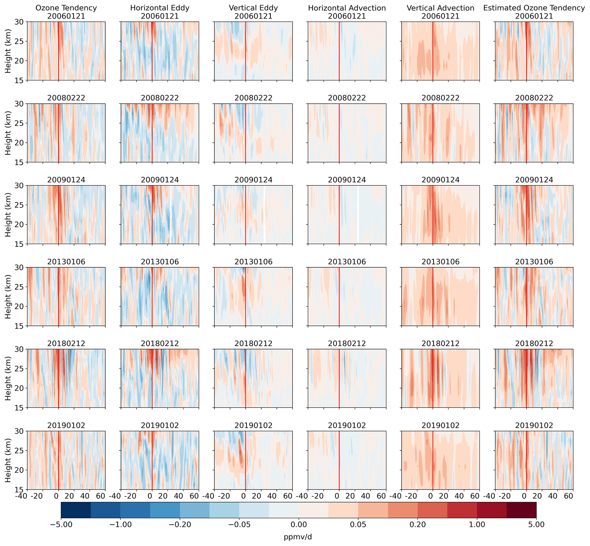
Figure 11Same as Fig. 8 for ozone tendency, horizontal and vertical component of eddy mixing, horizontal () and vertical () component of mean advection, and the indirect ozone tendency using the right-hand side of Eq. (2). Summing four middle columns leads to the estimated ozone tendency on the sixth column. The vertical axis is the log-pressure height.
The estimated ozone tendency (last column of Fig. 11) shows that using MERRA-2 fields, dynamical terms of tracer continuity can simulate the main features of the observed ozone tendency (first column of Fig. 11) from 15 to 30 km. We use these estimates to investigate the impact of different terms of tracer continuity on ozone. The key role of vertical advection and horizontal eddy mixing in ozone tendency is evident in Fig. 11. Vertical advection is the main driver of ozone tendency in the mid-stratosphere. Intensified residual circulation (Fig. 10) dramatically impacts the ozone increase. A significant signal of vertical advection is evident from 15 to 30 km in all six SSWs and is coincident with enhanced wave activity (Fig. 10), which is magnified around SSWs; however, it persists well after the vertical residual circulation signal disappears, up to 2 months after the SSWs. The sudden and intensified vertical advection is more magnified in 2009 and 2018, with an enduring elongated polar vortex.
Horizontal eddy mixing is the second important contributor in ozone tendency over the mid-stratosphere. While vertical advection builds up the ozone tendency, horizontal mixing tends to balance and weaken the ozone tendency. Increased wave activity and large-scale mixing drive a prolonged enhancement of the diffusivity of PV flux, which leads to increased horizontal eddy transport (Nakamura, 1996; de la Cámara et al., 2018a, b). Vertical eddy mixing has a clear signal above 20 km during minor and major SSWs. Horizontal advection has the least significant contribution to ozone tendency. The dominant contribution of vertical advection to mid-stratospheric ozone variability (15 to 30 km) using MERRA-2 dynamic parameters is consistent with climate model analysis (Tao et al., 2015; de la Cámara et al., 2018b). This study shows that the larger geographical extent and magnitude of ozone changes during SSWs with elongated polar vortex are tied to greater vertical advection during these events.
The time series of vertically integrated (15 to 30 km) ozone tendency, horizontal eddy mixing, vertical advection, and the residual of tracer continuity considering all terms in Eq. (2) are shown in Fig. 12. The major contribution of vertical advection to ozone tendency is evident in Fig. 12. The higher intensity of ozone tendency and vertical advection and their strong correlation coincident with the SSW date of the elongated polar vortex (2009 and 2018) stand out.

Figure 12Time series of vertically integrated major elements of tracer continuity (Eq. 2) from 15 to 30 km (Andrews et al., 1987). Ozone tendency is shown by the red line. The horizontal component of eddy mixing is shown by the blue line, and the vertical component of vertical advection is shown by the green line. The residual of all elements of tracer continuity is shown by the gray line.
Although the estimated ozone tendency (last column in Fig. 11) simulates most features of the observed ozone tendency (the first column in Fig. 11), they are not identical. The vertically integrated difference in observed and estimated ozone tendency is shown as the residual. The residual of tracer continuity results from both the numerical approximation of terms in Eq. (2) (errors in the horizontal derivatives over high latitude can be large as cos(φ) gets small) and the uncertainties in the balance of dynamical parameters in the reanalysis due to the data assimilation process (Martineau et al., 2018). Also, the possibility of chemical processes during splitting or displacement of the polar vortex out of the polar night region might contribute to the residual of tracer continuity. It should be noted that when viewing individual events, the plots are expected to be noisier than the average of numerous events.
SSWs are a major manifestation of disturbed stratospheric circulations. The altered dynamics influence the cycle of trace gases including ozone. The MERRA-2 reanalysis is used to investigate the influence of six persistent SSWs from 2004 to 2020 on ozone for the zonal average at high latitudes (60 to 80∘ N). The variability in impact of SSW on high-latitude ozone is analyzed, two different patterns are found, and possible related dynamical mechanisms are studied.
The comparison of the MERRA-2 ozone dataset with a unique density of observations at high latitudes provides an update to previous evaluations and provides understanding of the performance of MERRA-2 during high variability associated with extreme dynamical events such as SSWs. Comparisons are applied during December to May for each SSW. MERRA-2 shows good agreement with ozonesondes and FTIR observations in the middle stratosphere during highly altered dynamics of SSWs.
Comparison with ozonesondes at three high-latitude locations showed a mean difference ratio of 3 % (±7 %) in the stratosphere layer (10–30 km). However, the uncertainties are larger from the ground to 10 km. From 5 to 10 km, a negative mean bias exists in all sites (−8 % to 15 %); however, it is accompanied by a large standard deviation. Around 20 % standard deviation of relative differences is observed at G–5 km. A positive bias is observed at surface levels, where observations show depleted ozone due to bromine reactions.
Using a smoothing method, MERRA-2 is compared to five NDACC FTIR sites in four vertical layers (ground-8, 8–15, 15–22, and 22–30 km) during SSWs. These layers are defined based on the sensitivity of FTIR sensors. Overall, higher uncertainties are observed at the lowest level with 18 % SD. The best agreement is observed between 15–22 and 22–34 km with −2 % (±5 %) and −4 % (±5 %) mean (SD) relative differences. These results emphasize the high quality of MERRA-2 after August 2004, when MLS data are available, and motivate their usage in mid-stratospheric ozone analysis at high northern latitudes during highly disturbed dynamical events. Higher uncertainties in UTLS are also expected because MLS is a dominant contribution in MERRA-2 ozone profiles and has lower sensitivity at lower altitudes. Moreover, this study emphasizes the importance of independent ozone observations, such as ozonesondes and FTIR retrievals, as a means to evaluate models and assimilation estimations around the globe.
Using the MERRA-2 dataset, the variability of ozone changes during the SSWs and associated dynamic parameters are investigated. The evolution of the polar vortex and its impact on the ozone variability is studied using the average EPV at the potential temperature of 850 K. We identify two different patterns in the averaged polar vortex before the SSWs and the subsequent impact on ozone. In 2009 and 2018, an elongated polar vortex is observed before the SSWs which caused a predominantly negative ozone anomaly at northern high latitudes and is followed by an extensive positive ozone anomaly with large geographical extent. The TCO increase rates and the magnitude of changes in EPV after these cases are large, and the intrusion of positive temperature anomalies to the mid-stratosphere is coincident with these SSW dates.
During the SSWs in 2006, 2008, 2013, and 2019, the averaged polar vortex is displaced towards Europe, and the TCO exhibits positive anomalies before the SSWs in a large geographical region of northern high latitudes (outside the polar vortex). The positive TCO anomalies after the SSW have a smaller extent, and the magnitude of TCO variability and EPV change is smaller compared to observed changes during the elongated vortex events in 2009 and 2018. During these displaced events, the positive temperature anomalies in the middle stratosphere appear a few weeks before the SSW.
A strong correlation of R2=90 % is observed between the magnitude of change in the averaged EPV around the SSW and the magnitude of TCO change for the same period for all six studied SSWs plus two less persistent SSWs in 2007 and 2010. The regression analysis also emphasized the larger changes in both EPV and TCO during elongated SSWs.
The Greenland sector is one of the critical regions that is impacted by negative TCO anomalies before the elongated polar vortex in 2009 and 2018; positive TCO anomalies occur before displaced SSWs. To identify the similarities and differences of zonal versus the regional impact of SSWs on ozone, the analyses are applied over the Greenland sector as well as the zonal average. The general structure of the vertical ozone anomaly over the Greenland sector is similar to the zonal structure. However, as expected, the ozone anomaly over the zonal average is smoother than the Greenland sector, which results in a more magnified TCO increase over Greenland. The increased rate over the Greenland sector is between 15 % in 2006 and 38 % in 2018, while the zonal average ranges between 8 % in 2008 and 29 % in 2009.
We examined the dynamical terms associated with ozone tendency and investigated the evolution of ozone variability for each SSW using MERRA-2. The main features of observed mid-stratospheric ozone tendency are captured by the dynamical terms of the tracer continuity equation using MERRA-2 variables. Vertical advection is shown to be the main contributor of ozone tendency in the middle stratosphere during the SSWs and is more magnified during the enduring elongated polar vortex in 2009 and 2018. The impact of vertical advection coincides with the time of enhanced wave activity but can persist up to 2 months after the SSWs.
Suppressed wave activity initiates the recovery of temperature and ozone. However, the upper stratosphere experiences a faster recovery compared to the lower stratosphere because of the different radiative relaxation timescales (Randel et al., 2002). The fastest recovery of zonally averaged temperature and ozone at the middle stratosphere happens in 30 d for 2008. The positive ozone anomaly in the middle stratosphere lasts longer than the positive temperature anomaly in most of the SSWs by 10 d or more.
In conclusion, the MERRA-2 dataset is shown to capture the ozone variability in the middle stratosphere and provides dynamical information to investigate the impact of SSWs. This study shows that the averaged vortex shape before the SSWs is an important modulator of the magnitude and extent of ozone changes over high latitudes. The impact of SSWs on ozone is shown to be more intense in 2009 and 2018, with an elongated polar vortex, compared to the displaced vortices in 2006, 2008, 2013, and 2019. The magnitude of change in ozone is correlated with the magnitude of EPV change during the SSWs. The intensified vertical advection and abrupt wave forcing during elongated vortex events are tied to the more intense magnitude and larger geographical extent of ozone changes during these events. The addition of future SSW events could help to shed light on further details and to create more robust statistics regarding Arctic SSWs. Although there is no consensus across future climate simulations on whether SSW occurrences will increase or decrease in response to increased greenhouse gas concentration (Ayarzarguena et al., 2018, 2020), many simulations show a significant change. The dramatic ozone increases over high latitudes during SSWs point to the consequences and implications for ozone if the rate of SSW increases in future.
The code used to perform this analysis is available at https://doi.org/10.5281/zenodo.6466540 (Bahramvash Shams, 2022).
MERRA-2 data are provided by NASA at the Modeling and Assimilation Data and Information Services Center (MDISC) and are available in model level (GMAO, 2015a) at https://doi.org/10.5067/WWQSXQ8IVFW8 and in pressure level (GMAO, 2015b) at https://doi.org/10.5067/QBZ6MG944HW0. FTIR ozone retrieval datasets are provided by the Network for the Detection of Atmospheric Composition Change and are available at http://www.ndacc.org (NDACC, 2022). Ozonesonde data at Summit Station are provided by NOAA’s Earth System Research Laboratory through https://doi.org/10.7289/V5CC0XZ1 (Johnson et al., 2018). The rest of the ozonesonde measurements are provided by the World Ozone and Ultraviolet Radiation Data Centre (WOUDC) at https://doi.org/10.14287/10000001 (WMO/GAW Ozone Monitoring Community, 2013).
SBS performed the data processing and analysis and drafted and edited the paper. VPW conceived the project, provided advice on the data analysis, and aided in drafting and editing the paper. JWH provided NDACC FTIR data, advised the processing of FTIR data, and edited the paper. IVP provided ozonesonde profiles from Summit, advised the processing of in situ data, and edited the paper. WJR, AHB, and AdlC provided advice on analysis of atmospheric dynamics and edited the paper. All of the authors discussed the scientific findings and contributed to the paper and the revision.
The contact author has declared that neither they nor their co-authors have any competing interests.
Publisher's note: Copernicus Publications remains neutral with regard to jurisdictional claims in published maps and institutional affiliations.
We acknowledge NASA's Global Monitoring and Assimilation Office (GMAO) for providing the Modern-Era Retrospective analysis for Research and Applications, Version 2 (MERRA-2). We acknowledge the Ozone and Water Vapor Group at the Earth System Research Laboratory of the National Oceanic and Atmospheric Administration for use of the ozonesonde data and the science technicians at Summit Station, Greenland, for launching the ozonesondes. We acknowledge the World Ozone and Ultraviolet Radiation Data Centre (WOUDC) for providing Canadian and Norwegian ozonesondes. We acknowledge the Network for the Detection of Atmospheric Composition Change (NDACC) for providing trace gas retrievals from solar FTIRs. The authors are thankful to Kris Wargan and Simon Chabrillat for reviewing this paper and for their helpful comments.
This research has been supported by the National Science Foundation (grant nos. PLR-1420932 and PLR-1414314).
This paper was edited by Bernd Funke and reviewed by Simon Chabrillat and Kris Wargan.
Albers, J. R., Perlwitz, J., Butler, A. H., Birner, T., Kiladis, G. N., Lawrence, Z. D., Manney, G. L., Langford, A. O., and Dias, J.: Mechanisms Governing Interannual Variability of Stratosphere-to-Troposphere Ozone Transport, J. Geophys. Res., 123, 234–260, https://doi.org/10.1002/2017jd026890, 2018.
Ancellet, G., Daskalakis, N., Raut, J. C., Tarasick, D., Hair, J., Quennehen, B., Ravetta, F., Schlager, H., Weinheimer, A. J., Thompson, A. M., Johnson, B., Thomas, J. L., and Law, K. S.: Analysis of the latitudinal variability of tropospheric ozone in the Arctic using the large number of aircraft and ozonesonde observations in early summer 2008, Atmos. Chem. Phys., 16, 13341–13358, https://doi.org/10.5194/acp-16-13341-2016, 2016.
Andrews, D. G., Holton, J. R., and Leovy, C. B.: Middle atmosphere dynamics, Academic Press, edited by: Holton, J. R. and Dmowska, R., ISBN 13: 9780120585762, 1987.
Anstey, J. A. and Shepherd, T. G.: High-latitude influence of the quasi-biennial oscillation, Q. J. Roy. Meteor. Soc., 1, 1–21, https://doi.org/10.1002/qj.2132, 2014.
Ayarzagüena, B., Polvani, L. M., Langematz, U., Akiyoshi, H., Bekki, S., Butchart, N., Dameris, M., Deushi, M., Hardiman, S. C., Jöckel, P., Klekociuk, A., Marchand, M., Michou, M., Morgenstern, O., O'Connor, F. M., Oman, L. D., Plummer, D. A., Revell, L., Rozanov, E., Saint-Martin, D., Scinocca, J., Stenke, A., Stone, K., Yamashita, Y., Yoshida, K., and Zeng, G.: No robust evidence of future changes in major stratospheric sudden warmings: a multi-model assessment from CCMI, Atmos. Chem. Phys., 18, 11277–11287, https://doi.org/10.5194/acp-18-11277-2018, 2018.
Ayarzagüena, B., Charlton-Perez, A. J., Butler, A. H., Hitchcock, P., Simpson, I. R., Polvani, L. M., Butchart, N., Gerber, E. P., Gray, L., Hassler, B., Lin, P., Lott, F., Manzini, E., Mizuta, R., Orbe, C., Osprey, S., Saint-Martin, D., Sigmond, M., Taguchi, M., Volodin, E. M., and Watanabe, S.: Uncertainty in the Response of Sudden Stratospheric Warmings and Stratosphere-Troposphere Coupling to Quadrupled CO2 Concentrations in CMIP6 Models, J Geophys. Res.-Atmos., 125, e2019JD032345, https://doi.org/10.1029/2019jd032345, 2020.
Bahramvash Shams, S., Walden, V. P., Petropavlovskikh, I., Tarasick, D., Kivi, R., Oltmans, S., Johnson, B., Cullis, P., Sterling, C. W., Thölix, L., and Errera, Q.: Variations in the vertical profile of ozone at four high-latitude Arctic sites from 2005 to 2017, Atmos. Chem. Phys., 19, 9733–9751, https://doi.org/10.5194/acp-19-9733-2019, 2019.
Bahramvash Shams, S.: Analyzing Ozone and dynamical transport variables in middle stratosphere using MERRA-2 data (Jupiter notebook), Zenodo [code], https://doi.org/10.5281/zenodo.6466540, 2022.
Baldwin, M. P. and Dunkerton, T. J.: Stratospheric Harbingers of Anomalous Weather Regimes, Science, 294, 581–584, https://doi.org/10.1126/science.1063315, 2001.
Baldwin, M. P., Ayarzagüena, B., Birner, T., Butchart, N., Butler, A. H., Charlton-Perez, A. J., Domeisen, D. I. V., Garfinkel, C. I., Garny, H., Gerber, E. P., Hegglin, M. I., Langematz, U., and Pedatella, N. M.: Sudden Stratospheric Warmings, Rev. Geophys., 59, 27.1–37, https://doi.org/10.1029/2020rg000708, 2021.
Bognar, K., Zhao, X., Strong, K., Boone, C. D., Bourassa, A. E., Degenstein, D. A., Drummond, J. R., Duff, A., Goutail, F., Griffin, D., Jeffery, P. S., Lutsch, E., Manney, G. L., McElroy, C. T., McLinden, C. A., Millán, L. F., Pazmiño, A., Sioris, C. E., Walker, K. A., and Zou, J.: Updated validation of ACE and OSIRIS ozone and NO2 measurements in the Arctic using ground-based instruments at Eureka, Canada, J. Quant. Spectrosc. Ra., 238, 106571, https://doi.org/10.1016/j.jqsrt.2019.07.014, 2019.
Butler, A. H. and Domeisen, D. I. V.: The wave geometry of final stratospheric warming events, Weather Clim. Dynam., 2, 453–474, https://doi.org/10.5194/wcd-2-453-2021, 2021.
Butler, A. H., Seidel, D. J., Hardiman, S. C., Butchart, N., Birner, T., and Match, A.: Defining Sudden Stratospheric Warmings, B. Am. Meteor. Soc., 96, 1913–1928, https://doi.org/10.1175/bams-d-13-00173.1, 2015.
Butler, A. H., Sjoberg, J. P., Seidel, D. J., and Rosenlof, K. H.: A sudden stratospheric warming compendium, Earth Syst. Sci. Data, 9, 63–76, https://doi.org/10.5194/essd-9-63-2017, 2017.
Butler, A. H., Charlton-Perez, A., Domeisen, D. I. V., Garfinkel, C., Gerber, E. P., Hitchcock, P., Karpechko, A.-Y., Maycock, A. C., Sigmond, M., Simpson, I., and Son, S.-W.: Sub-seasonal Predictability and the Stratosphere, in: Chapter 11, The Gap Between Weather and Climate Forecasting, 223–241, https://doi.org/10.1016/B978-0-12-811714-9.00011-5, 2019.
Butler, A. H., Lawrence, Z. D., Lee, S. H., Lillo, S. P., and Long, C. S.: Differences between the 2018 and 2019 stratospheric polar vortex split events, Q. J. Roy. Meteor. Soc., 146, 3503–3521, https://doi.org/10.1002/qj.3858, 2020.
Cagnazzo, C. and E. Manzini.: Impact of the Stratosphere on the Winter Tropospheric Teleconnections between ENSO and the North Atlantic and European Region, J. Climate, 22, 1223–1238, https://doi.org/10.1175/2008JCLI2549.1, 2009.
Calvo, N., Polvani, L. M., and Solomon, S.: On the surface impact of Arctic stratospheric ozone extremes, Environ. Res. Lett., 10, 094003, https://doi.org/10.1088/1748-9326/10/9/094003, 2015.
de la Cámara, A., Abalos, M., and Hitchcock, P.: Changes in Stratospheric Transport and Mixing During Sudden Stratospheric Warmings, J. Geophys. Res., 123, 3356–3373, https://doi.org/10.1002/2017jd028007, 2018a.
de la Cámara, A., Abalos, M., Hitchcock, P., Calvo, N., and Garcia, R. R.: Response of Arctic ozone to sudden stratospheric warmings, Atmos. Chem. Phys., 18, 16499–16513, https://doi.org/10.5194/acp-18-16499-2018, 2018b.
de la Cámara, A., Birner, T., and Albers, J. R.: Are Sudden Stratospheric Warmings Preceded by Anomalous Tropospheric Wave Activity?, J. Climate, 32, 7173–7189, https://doi.org/10.1175/jcli-d-19-0269.1, 2019.
Charlton, A. J. and Polvani, L. M.: A New Look at Stratospheric Sudden Warmings. Part I: Climatology and Modeling Benchmarks, J. Climate, 20, 449–469, https://doi.org/10.1175/jcli3996.1, 2007.
Charlton-Perez, A. J., Ferranti, L., and Lee, R. W.: The influence of the stratospheric state on North Atlantic weather regimes, Q. J. Roy. Meteor. Soc., 144, 1140–1151, https://doi.org/10.1002/qj.3280, 2018.
Coy, L., Wargan, K., Molod, A. M., McCarty, W. R., and Pawson, S.: Structure and Dynamics of the Quasi-Biennial Oscillation in MERRA-2, J. Climate, 29, 5339–5354, https://doi.org/10.1175/jcli-d-15-0809.1, 2016.
Davis, S. M., Hegglin, M. I., Fujiwara, M., Dragani, R., Harada, Y., Kobayashi, C., Long, C., Manney, G. L., Nash, E. R., Potter, G. L., Tegtmeier, S., Wang, T., Wargan, K., and Wright, J. S.: Assessment of upper tropospheric and stratospheric water vapor and ozone in reanalyses as part of S-RIP, Atmos. Chem. Phys., 17, 12743–12778, https://doi.org/10.5194/acp-17-12743-2017, 2017.
Dickinson, R. E.: Method of parameterization for infrared cooling between altitudes of 30 and 70 kilometers, J. Geophys. Res., 78, 4451–4457, https://doi.org/10.1029/jc078i021p04451, 1973.
Flury, T., Hocke, K., Haefele, A., Kämpfer, N., and Lehmann, R.: Ozone depletion, water vapor increase, and PSC generation at midlatitudes by the 2008 major stratospheric warming, J. Geophys. Res., 114, 7903–14, https://doi.org/10.1029/2009jd011940, 2009.
Fritts, D. C. and Alexander, M. J.: Gravity wave dynamics and effects in the middle atmosphere, Rev. Geophys., 41, 1003, https://doi.org/10.1029/2001rg000106, 2003.
Fusco, A. C. and Salby, M. L.: Interannual Variations of Total Ozone and Their Relationship to Variations of Planetary Wave Activity, J. Climate, 12, 1619–1629, https://doi.org/10.1175/1520-0442(1999)012<1619:ivotoa>2.0.co;2, 1999.
García, O. E., Schneider, M., Redondas, A., González, Y., Hase, F., Blumenstock, T., and Sepúlveda, E.: Investigating the long-term evolution of subtropical ozone profiles applying ground-based FTIR spectrometry, Atmos. Meas. Tech., 5, 2917–2931, https://doi.org/10.5194/amt-5-2917-2012, 2012.
Gaudel, A., Ancellet, G., and Godin-Beekmann, S.: Analysis of 20 Years of tropospheric ozone vertical profiles by lidar and ecc at observatoire de Haute Provence (OHP) at 44∘ N, 6.7∘ E, Atmos. Environ., 113, 78–89, https://doi.org/10.1016/j.atmosenv.2015.04.028, 2015.
Gelaro, R., McCarty, W., Suárez, M. J., Todling, R., Molod, A., Takacs, L., Randles, C. A., Darmenov, A., Bosilovich, M. G., Reichle, R., Wargan, K., Coy, L., Cullather, R., Draper, C., Akella, S., Buchard, V., Conaty, A., Silva, A. M. da, Gu, W., Kim, G.-K., Koster, R., Lucchesi, R., Merkova, D., Nielsen, J. E., Partyka, G., Pawson, S., Putman, W., Rienecker, M., Schubert, S. D., Sienkiewicz, M., and Zhao, B.: The Modern-Era Retrospective Analysis for Research and Applications, Version 2 (MERRA-2), J. Climate, 30, 5419–5454, https://doi.org/10.1175/jcli-d-16-0758.1, 2017.
Global Modeling and Assimilation Office (GMAO), MERRA-2 inst3_3d_asm_Nv: 3d,3-Hourly,Instantaneous,Model-Level,Assimilation,Assimilated Meteorological Fields V5.12.4, Greenbelt, MD, USA, Goddard Earth Sciences Data and Information Services Center (GES DISC), https://doi.org/10.5067/WWQSXQ8IVFW8, 2015a.
Global Modeling and Assimilation Office (GMAO), MERRA-2 inst3_3d_asm_Np: 3d,3-Hourly,Instantaneous,Pressure-Level,Assimilation,Assimilated Meteorological Fields V5.12.4, Greenbelt, MD, USA, Goddard Earth Sciences Data and Information Services Center (GES DISC), https://doi.org/10.5067/QBZ6MG944HW0, 2015b.
Goncharenko, L. and Zhang, S.-R.: Ionospheric signatures of sudden stratospheric warming: Ion temperature at middle latitude, Geophys. Res. Lett., 35, L15804-4, https://doi.org/10.1029/2008gl035684, 2008.
Greening, K. and Hodgson, A.: Atmospheric analysis of the cold late February and early March 2018 over the UK, Weather, 74, 79–85, https://doi.org/10.1002/wea.3467, 2019.
Haigh, J. D.: The role of stratospheric ozone in modulating the solar radiative forcing of climate, Nature, 370, 544–546, https://doi.org/10.1038/370544a0, 1994.
Harada, Y., G. Atsushi, H. Hiroshi, and N. Fujikawa: A major stratospheric sudden warming event in January 2009, J. Atmos. Sci., 67, 2052–2069, https://doi.org/10.1175/2009JAS3320.1, 2010.
Hitchcock, P. and Simpson, I. R.: The Downward Influence of Stratospheric Sudden Warmings, J. Atmos. Sci., 71, 3856–3876, https://doi.org/10.1175/jas-d-14-0012.1, 2014.
Holton, J. R. and Lindzen, R. S.: An Updated Theory for the Quasi-Biennial Cycle of the Tropical Stratosphere, J. Atmos. Sci., 29, 1076–1080, https://doi.org/10.1175/1520-0469(1972)029<1076:autftq>2.0.co;2, 1972.
Holton, J. R., Haynes, P. H., McIntyre, M. E., Douglass, A. R., Rood, R. B., and Pfister, L.: Stratosphere-troposphere exchange, Rev. Geophys., 33, 403–439, https://doi.org/10.1029/95rg02097, 1995.
Houghton, J. T.: The stratosphere and mesosphere, Q. J. Roy. Meteor. Soc., 104, 1–29, https://doi.org/10.1002/qj.49710443902, 1978.
Ineson, S., and A. A. Scaife.: The role of the stratosphere in the European climate response to El Niño, Nat. Geosci., 2, 32–36, https://doi.org/10.1038/ngeo381, 2008.
Jaegleì, L., Wood, R., and Wargan, K.: Multiyear composite view of ozone enhancements and stratosphere-to-troposphere transport in dry intrusions of northern hemisphere extratropical cyclones, J. Geophys. Res.-Atmos., 122, 13436–13457, https://doi.org/10.1002/2017JD027656, 2017.
Johnson, B. J., Oltmans, S. J., Vömel, H., Smit, H. G. J., Deshler, T., and Kröger, C.: Electrochemical concentration cell (ECC) ozonesonde pump efficiency measurements and tests on the sensitivity to ozone of buffered and unbuffered ECC sensor cathode solutions, J. Geophys. Res., 107, 7881, https://doi.org/10.1029/2001jd000557, 2002.
Johnson, B. J., Cullis, P. D., and NOAA ESRL: Earth System Research Laboratory Ozone Water Vapor Group Ozonesonde Measurements, Version 1, NOAA National Centers for Environmental Information, https://doi.org/10.7289/V5CC0XZ1, 2018.
Karpechko, A. Y., Perlwitz, J., and Manzini, E.: A model study of tropospheric impacts of the Arctic ozone depletion 2011, J. Geophys. Res., 119, 7999–8014, https://doi.org/10.1002/2013jd021350, 2014.
Karpechko, A. Y., Perez, A. C., Balmaseda, M., Tyrrell, N., and Vitart, F.: Predicting Sudden Stratospheric Warming 2018 and Its Climate Impacts With a Multimodel Ensemble, Geophys. Res. Lett., 45, 13538–12546, https://doi.org/10.1029/2018gl081091, 2018.
Kidston, J., Scaife, A. A., Hardiman, S. C., Mitchell, D. M., Butchart, N., Baldwin, M. P., and Gray, L. J.: Stratospheric influence on tropospheric jet streams, storm tracks and surface weather, Nat. Geosci., 8, 1–8, https://doi.org/10.1038/ngeo2424, 2015.
Knowland, K. E., Ott, L. E., Duncan, B. N., and Wargan, K.: Stratospheric Intrusion-Influenced Ozone Air Quality Exceedances Investigated in the NASA MERRA-2 Reanalysis, Geophys. Res. Lett., 44, 10691–10701, https://doi.org/10.1002/2017gl074532, 2017.
Komhyr, W. D.: Operations handbook-ozone measurements to 40-km altitude with Model 4A Electrochemical Concentration Cell (ECC) ozonesonaes (used with 1680-MHz radiosondes), U.S. Dept. of Commerce, National Oceanic and Atmospheric Administration, Environmental Research Laboratories, Air Resources Laboratory, 1986.
Korenkov, Y. N., Klimenko, V. V., Klimenko, M. V., Bessarab, F. S., Korenkova, N. A., Ratovsky, K. G., Chernigovskaya, M. A., Shcherbakov, A. A., Sahai, Y., Fagundes, P. R., Jesus, R. de, Abreu, A. J. de, and Condor, P.: The global thermospheric and ionospheric response to the 2008 minor sudden stratospheric warming event, J. Geophys. Res., 117, A10309, https://doi.org/10.1029/2012ja018018, 2012.
Lawrence, Z. D. and Manney, G. L.: Does the Arctic Stratospheric Polar Vortex Exhibit Signs of Preconditioning Prior to Sudden Stratospheric Warmings?, J. Atmos. Sci., 77, 611–632, https://doi.org/10.1175/jas-d-19-0168.1, 2020.
Lee, S. H. and Butler, A. H.: The 2018–2019 Arctic stratospheric polar vortex, Weather, 75, 52–57, 2020.
Limpasuvan, V., Richter, J. H., Orsolini, Y. J., Stordal, F., and Kvissel, O.-K.: The roles of planetary and gravity waves during a major stratospheric sudden warming as characterized in WACCM, J. Atmos. Sol.-Terr. Phys., 78–79, 84–98, https://doi.org/10.1016/j.jastp.2011.03.004, 2012.
Lindzen, R. S. and Holton, J. R.: A Theory of the Quasi-Biennial Oscillation, J. Atmos. Sci., 25, 1095–1107, https://doi.org/10.1175/1520-0469(1968)025<1095:atotqb>2.0.co;2, 1968.
Logan, J. A.: Trends in the vertical distribution of ozone: An analysis of ozonesonde data, J. Geophys. Res., 99, 25, https://doi.org/10.1029/94jd02333, 1994.
Logan, J. A., Megretskaia, I. A., Miller, A. J., Tiao, G. C., Choi, D., Zhang, L., Stolarski, R. S., Labow, G. J., Hollandsworth, S. M., Bodeker, G. E., Claude, H., Muer, D. de, Kerr, J. B., Tarasick, D. W., Oltmans, S. J., Johnson, B., Schmidlin, F., Staehelin, J., Viatte, P., and Uchino, O.: Trends in the vertical distribution of ozone: A comparison of two analyses of ozonesonde data, J. Geophys. Res., 104, 26, https://doi.org/10.1029/1999jd900300, 1999.
Manney, G. L., Krüger, K., Pawson, S., Minschwaner, K., Schwartz, M. J., Daffer, W. H., Livesey, N. J., Mlynczak, M. G., Remsberg, E. E., Russel III, J. M., and Waters, J. W.: The evolution of the stratopause during the 2006 major warming: Satellite data and assimilated meteorological analyses, J. Geophys. Res., 113, D11115, https://doi.org/10.1029/2007jd009097, 2008a.
Manney, G. L., Daffer, W. H., Strawbridge, K. B., Walker, K. A., Boone, C. D., Bernath, P. F., Kerzenmacher, T., Schwartz, M. J., Strong, K., Sica, R. J., Krüger, K., Pumphrey, H. C., Lambert, A., Santee, M. L., Livesey, N. J., Remsberg, E. E., Mlynczak, M. G., and Russell III, J. R.: The high Arctic in extreme winters: vortex, temperature, and MLS and ACE-FTS trace gas evolution, Atmos. Chem. Phys., 8, 505–522, https://doi.org/10.5194/acp-8-505-2008, 2008b.
Manney, G. L., Schwartz, M. J., Krüger, K., Santee, M. L., Pawson, S., Lee, J. N., Daffer, W. H., Fuller, R. A., and Livesey, N. J.: Aura Microwave Limb Sounder observations of dynamics and transport during the record-breaking 2009 Arctic stratospheric major warming, Geophys. Res. Lett., 36, L12815, https://doi.org/10.1029/2009gl038586, 2009a.
Manney, G. L., Harwood, R. S., MacKenzie, I. A., Minschwaner, K., Allen, D. R., Santee, M. L., Walker, K. A., Hegglin, M. I., Lambert, A., Pumphrey, H. C., Bernath, P. F., Boone, C. D., Schwartz, M. J., Livesey, N. J., Daffer, W. H., and Fuller, R. A.: Satellite observations and modeling of transport in the upper troposphere through the lower mesosphere during the 2006 major stratospheric sudden warming, Atmos. Chem. Phys., 9, 4775–4795, https://doi.org/10.5194/acp-9-4775-2009, 2009b.
Manney, G. L., Lawrence, Z. D., Santee, M. L., Livesey, N. J., Lambert, A., and Pitts, M. C.: Polar processing in a split vortex: Arctic ozone loss in early winter 2012/2013, Atmos. Chem. Phys., 15, 5381–5403, https://doi.org/10.5194/acp-15-5381-2015, 2015.
Marsh, D. R., Mills, M. J., Kinnison, D. E., Lamarque, J.-F., Calvo, N., and Polvani, L. M.: Climate Change from 1850 to 2005 Simulated in CESM1(WACCM), J. Climate, 26, 7372–7391, https://doi.org/10.1175/jcli-d-12-00558.1, 2013.
Martineau, P., Wright, J. S., Zhu, N., and Fujiwara, M.: Zonal-mean data set of global atmospheric reanalyses on pressure levels, Earth Syst. Sci. Data, 10, 1925–1941, https://doi.org/10.5194/essd-10-1925-2018, 2018.
Matsuno, T.: A dynamical model of the stratospheric sudden warming, J. Atmos. Sci., 28, 1479–1494, https://doi.org/10.1175/1520-0469(1971)028<1479:ADMOTS>2.0.CO;2, 1971.
McDonald, M. K., Turnbull, D. N., and Donovan, D. P.: Steller Brewer, ozonesonde, and DIAL measurements of Arctic O3 column over Eureka, N.W.T. during 1996 winter/spring, Geophys. Res. Lett., 26, 2383–2386, https://doi.org/10.1029/1999gl900506, 1999.
Molod, A., Takacs, L., Suarez, M., and Bacmeister, J.: Development of the GEOS-5 atmospheric general circulation model: evolution from MERRA to MERRA2, Geosci. Model Dev., 8, 1339–1356, https://doi.org/10.5194/gmd-8-1339-2015, 2015.
Nakamura, N.: Two-Dimensional Mixing, Edge Formation, and Permeability Diagnosed in an Area Coordinate, J. Atmos. Sci., 53, 1524–1537, https://doi.org/10.1175/1520-0469(1996)053<1524:TDMEFA>2.0.CO;2, 1996.
Network for the Detection of Atmospheric Composition Change (NDACC): FTIR ozone retrievals, http://www.ndaccdemo.org/, last access: 18 April 2022.
Nowack, P. J., Abraham, N. L., Maycock, A. C., Braesicke, P., Gregory, J. M., Joshi, M. M., Osprey, A., and Pyle, J. A.: A large ozone-circulation feedback and its implications for global warming assessments, Nat. Clim. Chang., 5, 41–45, https://doi.org/10.1038/nclimate2451, 2015.
Palmeiro, F. M., Barriopedro, D., García-Herrera, R., and Calvo, N.: Comparing Sudden Stratospheric Warming Definitions in Reanalysis Data, J. Climate, 28, 6823–6840, https://doi.org/10.1175/jcli-d-15-0004.1, 2015.
Polvani, L. M. and Waugh, D. W.: Upward Wave Activity Flux as a Precursor to Extreme Stratospheric Events and Subsequent Anomalous Surface Weather Regimes., J. Climate, 17, 3548–3554, https://doi.org/10.1175/1520-0442(2004)017<3548:uwafaa>2.0.co;2, 2004.
Ramaswamy, V., Schwarzkopf, M. D., and Randel, W. J.: Fingerprint of ozone depletion in the spatial and temporal pattern of recent lower-stratospheric cooling, Nature, 382, 616–618, https://doi.org/10.1038/382616a0, 1996.
Randel, W. J.: Global variations of zonal mean ozone during strarospheric warming events, J. Atmos. Sci., 50, 3308–3321, 1993.
Randel, W. J., Wu, F., and Stolarski, R.: Changes in Column Ozone Correlated with the Stratospheric EP Flux, J. Meteorol. Soc. Jpn. Ser. II, 80, 849–862, https://doi.org/10.2151/jmsj.80.849, 2002.
Rao, J., Ren, R., Chen, H., Yu, Y., and Zhou, Y.: The Stratospheric Sudden Warming Event in February 2018 and its Prediction by a Climate System Model, J. Geophys. Res., 123, 13332–13345, https://doi.org/10.1029/2018jd028908, 2018.
Rao, J., Garfinkel, C. I., Chen, H., and White, I. P.: The 2019 New Year Stratospheric Sudden Warming and Its Real-Time Predictions in Multiple S2S Models, J. Geophys. Res., 124, 11155–11174, https://doi.org/10.1029/2019jd030826, 2019.
Rao, T. N.: Climatology of UTLS ozone and the ratio of ozone and potential vorticity over northern Europe, J. Geophys. Res., 108, 4703, https://doi.org/10.1029/2003jd003860, 2003.
Rao, T. N., Arvelius, J., Kirkwood, S., and Gathen, P. von der: Climatology of ozone in the troposphere and lower stratosphere over the European Arctic, Adv. Space Res., 34, 754–758, https://doi.org/10.1016/j.asr.2003.05.055, 2004.
Rienecker, M. M., Suárez, M. J., Gelaro, R., Todling, R., Bacmeister, J., Liu, E., Bosilovich, M. G., Schubert, S. D., Takacs, L., Kim, G.-K., Bloom, S., Chen, J., Collins, D., Conaty, A., Silva, A. da, Gu, W., Joiner, J., Koster, R. D., Lucchesi, R., Molod, A., Owens, T., Pawson, S., Pegion, P., Redder, C. R., Reichle, R., Robertson, F. R., Ruddick, A. G., Sienkiewicz, M., and Woollen, J.: MERRA: NASA's Modern-Era Retrospective Analysis for Research and Applications, J. Climate, 24, 3624–3648, https://doi.org/10.1175/jcli-d-11-00015.1, 2011.
Rodgers, C. D.: Inverse Methods for Atmospheric Sounding – Theory and Practice, Oxford, Series on Atmospheric Oceanic and Planetary Physics, https://doi.org/10.1142/9789812813718, 2000.
Rodgers, C. D. and Connor, B. J.: Intercomparison of remote sounding instruments, J. Geophys. Res., 108, 4116, https://doi.org/10.1029/2002jd002299, 2003.
Romanowsky, E., Handorf, D., Jaiser, R., Wohltmann, I., Dorn, W., Ukita, J., Cohen, J., Dethloff, K., and Rex, M.: The role of stratospheric ozone for Arctic-midlatitude linkages, Sci. Rep., 9, 1–7, https://doi.org/10.1038/s41598-019-43823-1, 2019.
Rothman, L. S., Gordon, I. E., Barbe, A., Benner, D. C., Bernath, P. F., Birk, M., Boudon, V., Brown, L. R., Campargue, A., Champion, J. P., Chance, K., Coudert, L. H., Dana, V., Devi, V. M., Fally, S., Flaud, J. M., Gamache, R. R., Goldman, A., Jacquemart, D., Kleiner, I., Lacome, N., Lafferty, W. J., Mandin, J. Y., Massie, S. T., Mikhailenko, S. N., Miller, C. E., Moazzen-Ahmadi, N., Naumenko, O. V., Nikitin, A. V., Orphal, J., Perevalov, V. I., Perrin, A., Predoi-Cross, A., Rinsland, C. P., Rotger, M., Šimečková, M., Smith, M. A. H., Sung, K., Tashkun, S. A., Tennyson, J., Toth, R. A., Vandaele, A. C., and Auwera, J. V.: The HITRAN 2008 molecular spectroscopic database, J. Quant. Spectrosc. Ra., 110, 533–572, https://doi.org/10.1016/j.jqsrt.2009.02.013, 2009.
Scheiben, D., Straub, C., Hocke, K., Forkman, P., and Kämpfer, N.: Observations of middle atmospheric H2O and O3 during the 2010 major sudden stratospheric warming by a network of microwave radiometers, Atmos. Chem. Phys., 12, 7753–7765, https://doi.org/10.5194/acp-12-7753-2012, 2012.
Scherhag, R.: Die explosionsartige Stratosphärenerwärmung des Spätwinters, Ber. Det. Wetterdienstes, 38, 51–63, 1952.
Schoeberl, M. R.: Stratospheric Warmings: Observations and Theory, 16, 521, https://doi.org/10.1029/rg016i004p00521, 1978.
Schranz, F., Hagen, J., Stober, G., Hocke, K., Murk, A., and Kämpfer, N.: Small-scale variability of stratospheric ozone during the sudden stratospheric warming 2018/2019 observed at Ny-Ålesund, Svalbard, Atmos. Chem. Phys., 20, 10791–10806, https://doi.org/10.5194/acp-20-10791-2020, 2020.
Scott, R. K. and Polvani, L. M.: Stratospheric control of upward wave flux near the tropopause, Geophys. Res. Lett., 31, L02115, https://doi.org/10.1029/2003gl017965, 2004.
Shangguan, M., Wang, W., and Jin, S.: Variability of temperature and ozone in the upper troposphere and lower stratosphere from multi-satellite observations and reanalysis data, Atmos. Chem. Phys., 19, 6659–6679, https://doi.org/10.5194/acp-19-6659-2019, 2019.
Siskind, D. E., Eckermann, S. D., Coy, L., McCormack, J. P., and Randall, C. E.: On recent interannual variability of the Arctic winter mesosphere: Implications for tracer descent, Geophys. Res. Lett., 34, 498–5, https://doi.org/10.1029/2007gl029293, 2007.
Smit, H. G. J., Straeter, W., Johnson, B. J., Oltmans, S. J., Davies, J., Tarasick, D. W., Hoegger, B., Stubi, R., Schmidlin, F. J., Northam, T., Thompson, A. M., Witte, J. C., Boyd, I., and Posny, F.: Assessment of the performance of ECC-ozonesondes under quasi-flight conditions in the environmental simulation chamber: Insights from the Juelich Ozone Sonde Intercomparison Experiment (JOSIE), J. Geophys. Res., 112, D19306, https://doi.org/10.1029/2006jd007308, 2007.
Smith, K. L. and Polvani, L. M.: The surface impacts of Arctic stratospheric ozone anomalies, Environ. Res. Lett., 9, 074015, https://doi.org/10.1088/1748-9326/9/7/074015, 2014.
Sterling, C. W., Johnson, B. J., Oltmans, S. J., Smit, H. G. J., Jordan, A. F., Cullis, P. D., Hall, E. G., Thompson, A. M., and Witte, J. C.: Homogenizing and estimating the uncertainty in NOAA's long-term vertical ozone profile records measured with the electrochemical concentration cell ozonesonde, Atmos. Meas. Tech., 11, 3661–3687, https://doi.org/10.5194/amt-11-3661-2018, 2018.
Stolarski, R. S.: History of the Study of Atmospheric Ozone, Ozone Science Engineering, 23, 421–428, https://doi.org/10.1080/01919510108962025, 2001.
Strahan, S. E., Douglass, A. R., and Steenrod, S. D.: Chemical and dynamical impacts of stratospheric sudden warmings on Arctic ozone variability, J. Geophys. Res.-Atmos, 121, 11836–11851, https://doi.org/10.1002/2016JD025128, 2016.
Tao, M., Konopka, P., Ploeger, F., Grooß, J.-U., Müller, R., Volk, C. M., Walker, K. A., and Riese, M.: Impact of the 2009 major sudden stratospheric warming on the composition of the stratosphere, Atmos. Chem. Phys., 15, 8695–8715, https://doi.org/10.5194/acp-15-8695-2015, 2015.
Tarasick, D. W. and Bottenheim, J. W.: Surface ozone depletion episodes in the Arctic and Antarctic from historical ozonesonde records, Atmos. Chem. Phys., 2, 197–205, https://doi.org/10.5194/acp-2-197-2002, 2002.
Tarasick, D. W., Davies, J., Smit, H. G. J., and Oltmans, S. J.: A re-evaluated Canadian ozonesonde record: measurements of the vertical distribution of ozone over Canada from 1966 to 2013, Atmos. Meas. Tech., 9, 195–214, https://doi.org/10.5194/amt-9-195-2016, 2016.
Tegtmeier, S., M. Rex, I. Wohltmann, and K. Krüger, Relative importance of dynamical and chemical contributions to Arctic wintertime ozone, Geophys. Res. Lett., 35, L17801, https://doi.org/10.1029/2008GL034250, 2008.
Thurairajah, B., Collins, R. L., Harvey, V. L., Lieberman, R. S., Gerding, M., Mizutani, K., and Livingston, J. M.: Gravity wave activity in the Arctic stratosphere and mesosphere during the 2007–2008 and 2008–2009 stratospheric sudden warming events, J. Geophys. Res., 115, D00N06, https://doi.org/10.1029/2010jd014125, 2010.
Tiao, G. C., Reinsel, G. C., Pedrick, J. H., Allenby, G. M., Mateer, C. L., Miller, A. J., and DeLuisi, J. J.: A statistical trend analysis of ozonesonde data, J. Geophys. Res., 91, 13121–13136, https://doi.org/10.1029/jd091id12p13121, 1986.
Tripathi, O. P., Baldwin, M., Perez, A. C., Charron, M., Eckermann, S. D., Gerber, E., Harrison, R. G., Jackson, D. R., Kim, B.-M., Kuroda, Y., Lang, A., Mahmood, S., Mizuta, R., Roff, G., Sigmond, M., and Son, S.-W.: The predictability of the extratropical stratosphere on monthly time-scales and its impact on the skill of tropospheric forecasts, Q. J. Roy. Meteor. Soc., 141, 987–1003, https://doi.org/10.1002/qj.2432, 2015.
Vigouroux, C., De Mazière, M., Demoulin, P., Servais, C., Hase, F., Blumenstock, T., Kramer, I., Schneider, M., Mellqvist, J., Strandberg, A., Velazco, V., Notholt, J., Sussmann, R., Stremme, W., Rockmann, A., Gardiner, T., Coleman, M., and Woods, P.: Evaluation of tropospheric and stratospheric ozone trends over Western Europe from ground-based FTIR network observations, Atmos. Chem. Phys., 8, 6865–6886, https://doi.org/10.5194/acp-8-6865-2008, 2008.
Vigouroux, C., Blumenstock, T., Coffey, M., Errera, Q., García, O., Jones, N. B., Hannigan, J. W., Hase, F., Liley, B., Mahieu, E., Mellqvist, J., Notholt, J., Palm, M., Persson, G., Schneider, M., Servais, C., Smale, D., Thölix, L., and De Mazière, M.: Trends of ozone total columns and vertical distribution from FTIR observations at eight NDACC stations around the globe, Atmos. Chem. Phys., 15, 2915–2933, https://doi.org/10.5194/acp-15-2915-2015, 2015.
Wallace, J. M.: General circulation of the tropical lower stratosphere, Rev. Geophys., 11, 191–222, https://doi.org/10.1029/rg011i002p00191, 1973.
Wargan, K., Labow, G., Frith, S., Pawson, S., Livesey, N., and Partyka, G.: Evaluation of the Ozone Fields in NASA's MERRA-2 Reanalysis, J. Climate, 30, 2961–2988, https://doi.org/10.1175/jcli-d-16-0699.1, 2017.
Wargan, K., Orbe, C., Pawson, S., Ziemke, J. R., Oman, L. D., Olsen, M. A., Coy, L., and Knowland, K. E.: Recent Decline in Extratropical Lower Stratospheric Ozone Attributed to Circulation Changes, Geophys. Res. Lett., 45, 5166–5176, https://doi.org/10.1029/2018gl077406, 2018.
WMO/GAW Ozone Monitoring Community: World Meteorological Organization-Global Atmosphere Watch Program (WMO-GAW)/World Ozone and Ultraviolet Radiation Data Centre (WOUDC), [data set], retrieved 24 October 2013, from https://woudc.org, https://doi.org/10.14287/10000001, 2013.
Xie, F., Li, J., Tian, W., Fu, Q., Jin, F.-F., Hu, Y., Zhang, J., Wang, W., Sun, C., Feng, J., Yang, Y., and Ding, R.: A connection from Arctic stratospheric ozone to El Niño-Southern oscillation, Environ. Res. Lett., 11, 124026–12, https://doi.org/10.1088/1748-9326/11/12/124026, 2016.