Assimilating spaceborne lidar dust extinction can improve dust forecasts

Atmospheric mineral dust has a rich tri-dimensional spatial and temporal structure that is poorly constrained in forecasts and analyses when only column-integrated aerosol optical depth (AOD) is assimilated. At present, this is the case of most operational global aerosol assimilation products. Aerosol vertical distributions obtained from spaceborne lidars can be assimilated in aerosol models, but questions about the extent of their benefit upon analyses and forecasts along with their consistency with AOD assimilation remain unresolved. Our study thoroughly explores the added value of assimilating spaceborne vertical dust profiles, with and without the joint assimilation of dust optical depth (DOD). We also discuss the consistency in the assimilation of both sources of information and analyse the role of the smaller footprint of the spaceborne lidar profiles in the results. To that end, we have performed data assimilation experiments using dedicated dust observations for a period of 2 months over northern Africa, the Middle East, and Europe. We assimilate DOD derived from the Visible Infrared Imaging Radiometer Suite (VIIRS) on board Suomi National Polar-Orbiting Partnership (SUOMI-NPP) Deep Blue and for the first time Cloud-Aerosol Lidar with Orthogonal Polarisation (CALIOP)-based LIdar climatology of Vertical Aerosol Structure for space-based lidar simulation studies (LIVAS) pure-dust extinction coefficient profiles on an aerosol model. The evaluation is performed against independent ground-based DOD derived from AErosol RObotic NETwork (AERONET) Sun photometers and ground-based lidar dust extinction profiles from the Cyprus Clouds Aerosol and Rain Experiment (CyCARE) and PREparatory: does dust TriboElectrification affect our ClimaTe (Pre-TECT) field campaigns. Jointly assimilating LIVAS and Deep Blue data reduces the root mean square error (RMSE) in the DOD by 39 % and in the dust extinction coefficient by 65 % compared to a control simulation that excludes assimilation. We show that the assimilation of dust extinction coefficient profiles provides a strong added value to the analyses and forecasts. When only Deep Blue data are assimilated, the RMSE in the DOD is reduced further, by 42 %. However, when only LIVAS data are assimilated, the RMSE in the dust extinction coefficient decreases by 72 %, the largest improvement across experiments. We also show that the assimilation of dust extinction profiles yields better skill scores than the assimilation of DOD under an equivalent sensor footprint. Our results demonstrate the strong potential of future lidar space missions to improve desert dust forecasts, particularly if they foresee a depolarization lidar channel to allow discrimination of desert dust from other aerosol types.

1 Introduction

The spatial and temporal distribution of atmospheric aerosol can be optimally estimated by combining observations and numerical models using data assimilation (DA) techniques. The resulting fields, referred to as aerosol analyses, serve as initial conditions for aerosol forecasting. Long-term and consistent analyses, so-called aerosol reanalyses, are useful for investigating aerosol variability, trends, impacts, and climate feedbacks, and they are produced with the same DA techniques (Benedetti et al., 2009; Lynch et al., 2016; Randles et al., 2017; Yumimoto et al., 2017; Inness et al., 2019; Di Tomaso et al., 2021).

A key uncertainty in current models is the representation of the aerosol vertical distribution (Pérez et al., 2006; Koffi et al., 2016; Benedetti et al., 2018; Konsta et al., 2018). Most operational aerosol forecast systems rely on the assimilation of column-integrated aerosol optical depth (AOD) from satellite-borne instruments (e.g. Xian et al., 2019). Consequently, the vertical structure is mainly propagated from the numerical model and only slightly and indirectly from the assimilated observations. In the last decade, a few studies have investigated the assimilation of vertical aerosol profiles from lidar instruments, both satellite (e.g. Cloud-Aerosol Lidar with Orthogonal Polarisation (CALIOP), Winker et al., 2010) and ground-based (e.g. European Aerosol Research Lidar Network (EARLINET), Pappalardo et al., 2014), showing the potential of vertical profiling to improve the four-dimensional representation of aerosols in analyses (Sekiyama et al., 2010; Zhang et al., 2011; Wang et al., 2014; Kahnert and Andersson, 2017; Cheng et al., 2019; El Amraoui et al., 2020) and forecasts (Zhang et al., 2011; Wang et al., 2014). Difficulties preventing an effective assimilation of vertical profiles in operational settings include the poor coverage of ground-based observations, the narrow footprint of satellite observations, potential inconsistencies with other assimilated observations, and underrepresented forecasting uncertainty in the vertical, among others.

Our study focuses on the assimilation of desert dust aerosol lidar observations around the two most prolific source regions on Earth: northern Africa and the Middle East. Dust models are subject to substantial uncertainties in the description of lower boundary conditions relevant for dust emission, modelled wind speed, dust emission processes, vertical mixing, particle properties, and deposition (Huneeus et al., 2011; Kok et al., 2021; Klose et al., 2021a). Thus, combining modelling with dust observations through DA is a powerful method to increase the quality of emission estimates (Escribano et al., 2016, 2017) and dust forecasts. We are specifically interested here in the impact of assimilating spaceborne lidar profiles upon dust forecasts. Dust is the largest continental contributor to the global aerosol load and impacts marine (Jickells et al., 2005) and land biogeochemistry (Okin et al., 2004), radiative fluxes (DeMott et al., 2009; Kok et al., 2017; Marinou et al., 2019), human health (Du et al., 2015), and the economy (Kosmopoulos et al., 2018; Papagiannopoulos et al., 2020). Properly representing its vertical structure both within the planetary boundary layer over sources and in the free troposphere in the outflow areas is particularly important for predicting its long-range transport and associated impacts (O'Sullivan et al., 2020). Despite this important role, the dust vertical structure in models and forecasts is poorly constrained by observations (Benedetti et al., 2014). So far, only lidar measurements, either from space or from ground, can deliver vertical profiles of the atmospheric dust.

Our work involves both modelling and data assimilation aspects along with the handling of observations and their uncertainty. We use the Multiscale Online Non-hydrostatic AtmospheRe CHemistry (MONARCH) model, formerly known as NMMB/BSC-Dust (Pérez et al., 2011; Klose et al., 2021a), enhanced with a local ensemble transform Kalman filter data assimilation capability (Di Tomaso et al., 2017). MONARCH provides dust forecasts at the World Meteorological Organization (WMO) Sand and Dust Storm Warning Advisory and Assessment System (SDS-WAS) regional centres for northern Africa, the Middle East, and Europe (http://sds-was.aemet.es/, last access: 11 November 2021; http://dust.aemet.es/, last access: 11 November 2021) hosted by the Spanish Meteorological Agency (AEMET) and the Barcelona Supercomputing Center (BSC). We address the challenge of how to best express model uncertainty also in the vertical coordinate and consequently in the dust transport, generating an ensemble for MONARCH based on both meteorological and dust source perturbations. Rubin et al. (2016) showed that combining meteorology and aerosol source ensembles produces sufficient spread in outflow regions that positively impacts the results. Characterizing model uncertainty is key to effectively assimilating observations; spatial and multivariate structures of the error background covariance determine the spread of observational information in space and across variables, allowing for statistically consistent increments between neighbouring grid points, also along the vertical dimension. The use of an ensemble-based data assimilation scheme, such as the one used in this work, allows for background covariances to evolve with the forecast.

Assimilating dust in models is possible to the extent that there are dust-specific retrievals with suitable coverage, quality, and uncertainty quantification. Progress has been made recently to provide dust products from satellite-borne spectroradiometers in the visible (e.g. Pu and Ginoux, 2016; Zhou et al., 2020b, a), from the Infrared Atmospheric Sounding Interferometer (IASI) (e.g. Capelle et al., 2018; Clarisse et al., 2019), from ground and satellite-based lidar instruments (Mamouri and Ansmann, 2014; Amiridis et al., 2015), or from combinations of reanalyses with satellite retrievals (Gkikas et al., 2021). In our study we assimilate pixels with dust retrievals from the Visible Infrared Imaging Radiometer Suite (VIIRS) Deep Blue AOD product (Hsu et al., 2019) along with LIdar climatology of Vertical Aerosol Structure for space-based lidar simulation studies (LIVAS) pure-dust extinction coefficient profiles from CALIOP as described in Amiridis et al. (2013, 2015) and Marinou et al. (2017). Finally, our analyses and analysis-initialized forecasts are evaluated against independent observations, namely dust-filtered AOD from ground-based AErosol RObotic NETwork (AERONET) observations and lidar dust extinction coefficient profiles collected during the PREparatory: does dust TriboElectrification affect our ClimaTe (Pre-TECT, http://pre-tect.space.noa.gr, last access: 11 November 2021) and Cyprus Clouds Aerosol and Rain Experiment (CyCARE, Radenz et al., 2017) campaigns between 19 and 23 April 2017.

The paper is organized as follows. In Sect. 2 we describe the data and methods employed in this study. In Sect. 3 we investigate the potential improvements in the representation of the dust vertical structure by assimilating dust-dedicated profiling information in a close-to-optimal data assimilation framework. We also assess the overall benefit of applying constraints on both the dust total column extinction and the dust extinction profile. Finally, we compare vertically resolved versus column-integrated data assimilation under comparable temporal and spatial geographical sampling. Section 4 concludes the paper, highlighting the main results obtained.

2 Data and methods

We performed data assimilation experiments to evaluate the impact of assimilating satellite products of dust optical depth (DOD) and vertically resolved dust extinction coefficient, either alone or in combination. These two datasets are described in Sect. 2.1. The experiments were evaluated against independent ground-based Sun photometer and lidar observations that are described in Sect. 2.2. The modelling and data assimilation systems, described in Sect. 2.3 and 2.4 respectively, were optimized in a number of respects, including the generation of ensemble perturbations, the spatial and temporal localization that creates a smooth limit upon the observation influence in the analysis fields, and the optical properties used in the observation operator. A description of the experiments and their evaluation are provided in Sect. 2.5

2.1 Assimilated observations

2.1.1 CALIOP-based LIVAS dataset

Pure-dust profiles assimilated in this study were derived from the global three-dimensional European Space Agency (ESA) LIVAS database (Amiridis et al., 2013, 2015). LIVAS is based on multiyear CALIPSO (Cloud-Aerosol Lidar and Infrared Pathfinder Satellite Observations, Winker et al., 2009) CALIOP aerosol observations. In this work, we use the LIVAS pure-dust extinction coefficient product, derived at CALIPSO Level 2 with a vertical resolution of 60 m and a horizontal resolution of 5 km. The methodology of LIVAS to retrieve the pure-dust extinction coefficient from CALIPSO uses the depolarization-based separation method introduced by Shimizu et al. (2004) and Tesche et al. (2009), coupled with a regionally suitable climatological lidar ratio. The latter is estimated from long-term EARLINET measurements (e.g. 55 sr for the Sahara, 40 sr for the Middle East) (Baars et al., 2016). It has been shown that the LIVAS dust product presented in Amiridis et al. (2013) and later updated in Marinou et al. (2017) is in good agreement with AERONET-collocated measurements, with an absolute AOD bias of the order of ∼0.03.

Accordingly, and prior to assimilation, the profiles of the LIVAS pure-dust extinction coefficient at 532 nm were aggregated to the horizontal resolution of the model. In the regridding process, error definitions and filtering of CALIOP profiles followed procedures similar to Cheng et al. (2019). More specifically, Cheng et al. (2019) used CALIOP optical products under the condition that at least 20 CALIOP L2 profiles were provided in each 2^∘ × 2^∘ model grid cell. Considering the finer model grid resolution of 0.66^∘ × 0.66^∘ of the present study – in an analogous approach to Cheng et al. (2019) – a threshold of at least three quality-assured (QA) cloud-free (CF) CALIOP L2 profiles was set, achieving a similar proportion of horizontal geographical coverage to Cheng et al. (2019). Similar was the filtering approach followed for the coefficient of variation (standard deviation divided by mean) of the data prior to regridding, although it was less restrictive due to the smaller number of profiles and the higher spatial resolution of the model grid. More specifically, only grid cells with a coefficient of variation less than unity were used in the assimilation, while in Cheng et al. (2019) the corresponding threshold was set equal to 0.5.

In addition, in order to avoid spurious values in the assimilation process (e.g. unrealistic high values of the extinction coefficient at 532 nm arising from possible misclassification of clouds as aerosols), we discarded LIVAS dust extinction coefficients larger than ${\mathrm{10}}^{-\mathrm{3}}{\mathrm{m}}^{-\mathrm{1}}$. Errors in LIVAS pure-dust extinction coefficient profiles are of the order of 20 %–54 % (Marinou et al., 2017). In consequence, and similarly to Cheng et al. (2019), input error statistics for the data assimilation routine were prescribed as 20 % of the value of the dust extinction coefficient. An additional filter was applied to ensure that the 60 m vertical-resolution observations cover at least half of each model layer vertical thickness. Model layer thickness is defined by the model hybrid pressure–sigma coordinate; its value is not homogeneous in the vertical: it varies between 16 and 61 m close to the surface depending on the topography, between about 140 and 750 m at 6.5 km altitude and between 540 and 640 m at 10 km height. Model layers and the corresponding LIVAS observations with less than 50 % of vertical coverage were omitted in the observation operator. The remaining observations were averaged and the associated uncertainty was computed assuming a Gaussian correlation length of 1 km in the vertical coordinate for each model layer independently.

2.1.2 VIIRS Deep Blue dataset

The DOD at 550 nm was extracted from the Deep Blue (DB) Level-2 product of the VIIRS instrument on board the Suomi National Polar-Orbiting Partnership (SUOMI-NPP) satellite (Sayer et al., 2018; Hsu et al., 2019). The DB product provides total AOD at 550 nm with a global coverage daily. Along with AOD, the DB product includes a flag with the aerosol-type classification of the retrieval (namely dust, smoke, high-altitude smoke, non-smoke fine-dominated, mixed, background, and fine-mode-dominated) and quality-assurance flags over ocean and land from 1 (worst quality) to 3 (best quality). Hsu et al. (2019) highlight the improvements done in the DB retrieval for dust aerosols, as the optical model was updated with non-spherical dust optical properties.

The standard DB product is AOD. We used only pixels classified as “dust” aerosol type and with a quality assurance flag equal to 3 over the ocean and greater than or equal to 2 over land. The resulting DOD dataset was then interpolated to the model grid and assigned an uncertainty of $\mathrm{0.2}\times \text{DOD}+\mathrm{0.05}$ following Sayer et al. (2019). Hereafter we use DDB to refer to this filtered dust DB retrieval. We note that DDB is not necessarily a pure-dust AOD and may include contributions of other aerosol types, although dust should be predominant, particularly in northern Africa and the Middle East.

The large swath (∼3040 km) of the VIIRS instrument can be a big plus for data assimilation. In contrast, CALIOP has a horizontal footprint of 100 m and a horizontal resolution of 333 m. When comparing the assimilation from both instruments, it is key to understanding the role of these differences in spatial coverage. To respond to this fundamental question, we prepared a subset of DDB data, called hereafter DDBsubset, that contains the (regridded) DOD from DDB collocated with LIVAS. This collocation is done at a daily resolution and in the horizontal model grid (which is the same horizontal grid of DBB and LIVAS after the processing described in the previous paragraphs). For each UTC day, we create a bi-dimensional binary mask whose values are set to valid only when the LIVAS dataset has a valid retrieval in at least one vertical level for that UTC day. This daily mask is applied to DDB to create DDBsubset.

2.2 Ground-based observations for evaluation

2.2.1 AERONET

We used ground-based measurements for the evaluation. For DOD, we selected the group of AERONET stations (Holben et al., 1998) used in the operational SDS-WAS verification. The list of stations is presented in Appendix A. We used the AERONET Direct Sun product, version 3, level 2. The AOD was interpolated to 550 nm, and we assumed dust to be predominant when Ångström exponents at 440–870 nm were smaller than 0.3 (Basart et al., 2009). In a similar fashion to the AOD filter used in DDB, this filtered AERONET dataset is not a pure-dust AOD. Nevertheless, it is expected that the main aerosol type in the vertical column of this AERONET-filtered dataset is dust, but it can be mixed with other types of aerosols (as for example coarse sea spray).

2.2.2 Ground-based lidar CyCARE and Pre-TECT campaigns

The modelled vertical profiles of the dust extinction coefficient at 532 nm were evaluated against measurements from three ground-based lidars of the lidar network PollyNET (Baars et al., 2016; Engelmann et al., 2016) operated in the eastern Mediterranean during the CyCARE and Pre-TECT experiments. These lidars were located at Finokalia, Crete, Greece (operated by the National Observatory of Athens, NOA), Limassol, Cyprus (operated by the Leibniz Institute for Tropospheric Research, TROPOS, in the framework of CyCARE), and Haifa, Israel (Althausen et al., 2019, operated by TROPOS). With these continuously operating lidars, the vertical profiles of the particle backscatter coefficient at 355, 532, and 1064 nm, the extinction coefficient at 355 and 532 nm, and the particle depolarization ratio at 355 and 532 nm can be retrieved. Using the obtained particle backscatter coefficient, extinction coefficient, and depolarization ratio at 532 nm, the dust-only extinction coefficient can be obtained as described in Mamouri and Ansmann (2014, 2017). With this method, the backscatter-related dust fraction is calculated based on the known depolarization ratio of pure dust (31 %) and the non-dust component (5 %). Having the dust-only backscatter coefficient, the dust-only extinction coefficient is determined by the use of the pure dust lidar ratio at 532 nm of 45 sr (Mamouri and Ansmann, 2016). The non-dust extinction coefficient is calculated similarly depending on the type of non-dust aerosol. Finally, a consistency check is performed by summing up the dust-only and non-dust extinction profiles and comparing them to the total measured extinction coefficient. More details can be found in Urbanneck (2018).

In contrast to the estimated DOD from AERONET and DB AOD retrievals, which may be affected by other aerosols, the PollyNET measurements can provide pure-dust retrievals (Tesche et al., 2009; Mamouri and Ansmann, 2017). For this reason, we use here the lidar observations from the CyCARE and Pre-TECT campaigns in the evaluation of our results.

2.3 MONARCH model

To simulate the dust cycle, we used the Multiscale Online Nonhydrostatic AtmospheRe CHemistry (MONARCH) model (Pérez et al., 2011; Haustein et al., 2012; Jorba et al., 2012; Badia et al., 2017; Di Tomaso et al., 2017; Klose et al., 2021a). MONARCH is a fully online integrated system for meso- to global-scale applications developed at the BSC. It uses the Nonhydrostatic Multiscale Model on the B-grid (NMMB, Janjic and Gall, 2012) as the meteorological driver and couples gas-phase and mass-based aerosol modules to describe the life cycle of atmospheric components. It uses the Autosubmit workflow manager (Manubens-Gil et al., 2016), which is particularly useful for efficiently executing assimilation runs. The model provides operational regional mineral dust forecasts at WMO SDS-WAS regional centres. It has also contributed global aerosol forecasts within the multimodel ensemble of the International Cooperative for Aerosol Prediction (ICAP) initiative (Xian et al., 2019) since 2012 and will soon integrate the Copernicus Atmosphere Monitoring Service (CAMS) – Air Quality Regional Production (https://www.regional.atmosphere.copernicus.eu, last access: 11 November 2021).

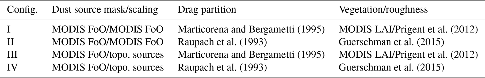
MONARCH contains comprehensive aerosol and chemistry packages, but in this work we only focus on and compute mineral dust aerosol. Dust is described using eight particle-size bins within 0.2–20 µm in diameter. The MONARCH dust module is described in detail in Pérez et al. (2011) and Klose et al. (2021a). MONARCH offers a diversity of mineral dust emission schemes along with multiple configurations. As shown in Klose et al. (2021a), the emission scheme and their specific configuration have a strong impact on the spatial and temporal behaviour of the simulated dust. Because we aim at showing the impact on the forecast by assimilating two different types of observations and not at showing the best of the forecasts, we preferred to avoid fine-tuning and cherry-picking the best-performing emission scheme and configuration for our study case. Instead, we computed dust emissions by averaging the emissions produced by the four configurations listed in Table 1. All the configurations used a modified version of the dust emission scheme of Ginoux et al. (2001) with modifications described in Klose et al. (2021a) that include the use of friction velocity instead of 10 m wind speed, a dust-particle size-independent threshold friction velocity for particle entrainment taken as the minimum value of the threshold function from Shao and Lu (2000), and an emitted size distribution following Kok (2011). The entrainment threshold accounts for soil moisture using the correction from Belly (1964) as described in Ginoux et al. (2001). Areas where dust emission is allowed are constrained by satellite observations, specifically by the frequency of occurrence (FoO) of the Moderate Resolution Imaging Spectroradiometer (MODIS) DB DOD exceeding 0.2 (Hsu et al., 2004; Ginoux et al., 2012). Dust can be emitted for areas in which FoO >0.025 (Klose et al., 2021a). The four configurations differ with regard to the description of (a) the preferential dust sources used for scaling of the dust emission flux and (b) vegetation and surface roughness effects. Configurations I and II used the MODIS FoO of DOD >0.2 to scale the dust emission flux obtained with the modified Ginoux et al. (2001) parameterization. Configurations III and IV used the original topographic source mask from Ginoux et al. (2001) as the scaling function. To account for roughness elements on the land surface, such as vegetation, rocks, or pebbles, configurations I and III used the drag partition parameterization from Marticorena and Bergametti (1995) with corrections from King et al. (2005) in combination with a monthly climatology of MODIS-derived leaf-area index (Myeni et al., 2015) and aerodynamic roughness length data for arid regions from Prigent et al. (2012). In contrast, configurations II and IV utilized the drag partition parameterization from Raupach et al. (1993) together with a monthly climatology of photosynthetic and non-photosynthetic vegetation cover data from Guerschman et al. (2015) (Klose et al., 2021a). The drag partition corrections were applied to the threshold friction velocity for particle entrainment.

Marticorena and Bergametti (1995)Prigent et al. (2012)Raupach et al. (1993)Guerschman et al. (2015)Marticorena and Bergametti (1995)Prigent et al. (2012)Raupach et al. (1993)Guerschman et al. (2015)

Table 1 Summary of the four model configurations used to create the multi-scheme dust emissions.

2.4 Data assimilation

MONARCH is coupled to a local ensemble transform Kalman filter (LETKF, Hunt et al., 2007). The LETKF implementation used in this study was built upon the implementation from Miyoshi and Yamane (2007), Schutgens et al. (2010), and Di Tomaso et al. (2017). We used the 4D-LETKF configuration of this code with an assimilation window and forecast length of 24 h (starting at 00:00 UTC) and with hourly outputs. In this LETKF implementation, the observations had been compared to the model-simulated equivalent observations with collocation in time and space and then concatenated to construct the observation and the simulated observation vectors. An ensemble of MONARCH runs is used to estimate the error covariance matrix of the prior at the observations' times and locations. We used a Gaussian localization with a horizontal scale of six grid cells (around 435 km in our model configuration), a vertical scale of one model level, and a temporal scale of 12 h. Unlike Di Tomaso et al. (2017) or Cheng et al. (2019), we computed the analysis every hour instead of only at 00:00 UTC. With this configuration, the 4D-LETKF acts as a Kalman smoother that effectively localizes the influence of the observations in time and therefore produces better-quality analyses throughout the 24 h assimilation window. This choice is advantageous when the assimilated observations are temporally distributed along the assimilation window like in the case of LIVAS with daytime and nighttime profiles or when the observations are more representative of local conditions, as is the case of extinction coefficients compared to column-integrated AOD values. In comparison with Di Tomaso et al. (2017) and Cheng et al. (2019), the Kalman smoother choice described above should provide the same analyses at 00:00 UTC as the filtering option. Therefore, the analysis-initialized forecasts are identical with both approaches.

A key ingredient in the data assimilation algorithm is the representation of model uncertainty, which in an ensemble-based scheme, like ours, had been derived from the model ensemble. We have generated the MONARCH ensemble by perturbing dust emissions and by using an ensemble of meteorological initial and boundary condition analyses (Global Ensemble Forecast System (GEFS), Zhou et al., 2017). The model ensemble was constructed with 20 members, concordant with the 20 GEFS ensemble members. The dust emissions in the model (Sect. 2.3) were perturbed by multiplicative factors that were extracted from a random Gaussian distribution with a spatial correlation of 250 km, a mean of unity, and a standard deviation of 0.4. In all cases we assumed that the observational errors were uncorrelated, i.e. that the observational error covariance matrix was a diagonal matrix.

2.5 Experiment description and evaluation

We describe in Sect. 2.1 the three datasets used in the assimilation: DDB, DDBsubset, and LIVAS. Using a fixed configuration of the model and the data assimilation scheme parameters (Sect. 2.3 and 2.4), we designed and ran five experiments assimilating combinations of the three datasets.

The first experiment, named eLIVAS, assimilated the pure-dust extinction coefficient from the regridded LIVAS dataset (Sect. 2.1.1). A second experiment, named eDDB, assimilated the DOD from the DDB dataset (Sect. 2.1.2). The third experiment, named eDDBsubset, assimilated the DDBsubset dataset (Sect. 2.1.2). The fourth, named eLIVAS+DDBsubset, assimilated the LIVAS and DDBsubset datasets, and the fifth, named eLIVAS+DDB, assimilated the LIVAS and DDB datasets. For the sake of clarity, we have excluded DDBsubset experiments until Sect. 3.3. Therefore, until Sect. 3.3, we will focus on results of eLIVAS, eDDB, and eLIVAS+DDB experiments.

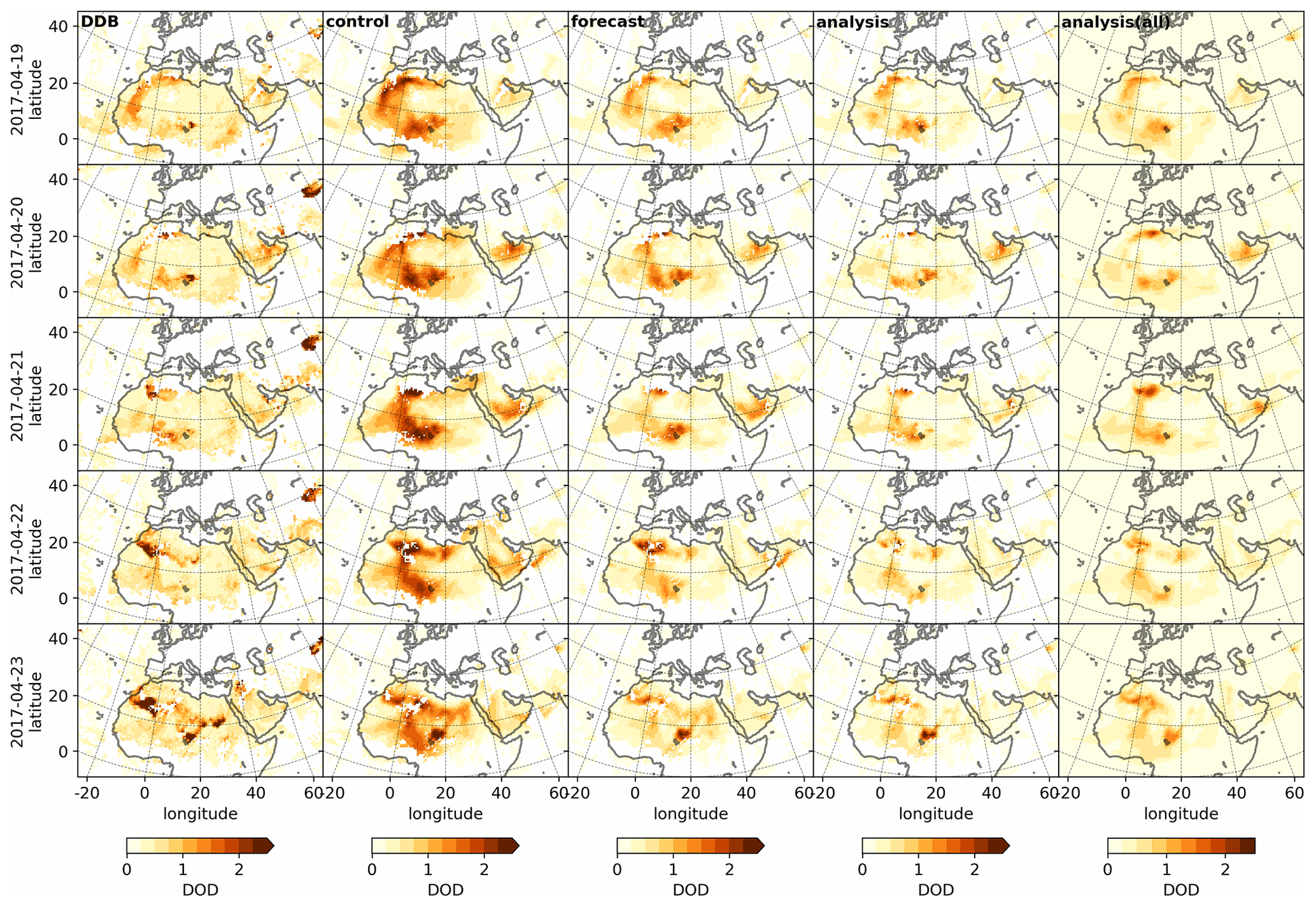
Figure 1 DOD from DDB and model simulations between 19 and 23 April 2017 for the control and eLIVAS experiments. The first four columns show the DOD from DDB (left) and three model simulations of DOD collocated with DDB: control experiment, forecast, and analysis from the eLIVAS experiment. The last column shows the analyses' daily average without collocation with DDB. Each row represents a different day.

We ran our data assimilation experiments over a regional domain centred at 20^∘ E in longitude and 30^∘ N in latitude, which covers northern Africa, the Middle East, and Europe (e.g. Fig. 1). The model was set up with a rotated latitude–longitude grid with 0.66^∘ resolution at the centre of the grid, 40 vertical layers, and hourly output of dust concentrations for the eight size bins. The dust extinction coefficient and DOD were computed with software provided by Gasteiger and Wiegner (2018). We have assumed spheroidal dust particles with the axis ratio distribution shown in Table 2 of Koepke et al. (2015) and the OPAC refractive index for dust (e.g. 1.53+0.0055i for 550 nm) as in Koepke et al. (2015).

We performed the five data assimilation experiments between March and April 2017. A 14-month spin-up was run without assimilation to properly initialize the soil moisture content. We also ran a control experiment over the period of study, consisting of an ensemble forecast without data assimilation. For each of the five data assimilation experiments (eLIVAS, eDDB, eDDBsubset, eLIVAS+DDBsubset, and eLIVAS+DDB), we obtained two types of simulation outputs: analyses and forecasts.

We produced ensemble forecasts with a forecast length of 24 h, initialized with the last time step of the analyses of the day before (at 00:00 UTC in our 24 h assimilation window). Forecasts and observations along with their prescribed error were the input for the data assimilation scheme, which computed the four-dimensional mass concentration dust field analyses within the assimilation window. Therefore, for a given day, forecasts can carry the observational information assimilated from the days before, but analyses can, in addition, carry the observational information of that given day. In contrast, the control experiment omits the assimilation of dust information.

When comparing the model against observations, the model was always collocated in space and time with the valid observations. In the case of ground-based lidar observations, the model is integrated in time over the measurement window. To summarize the comparison between model and observations, we have computed six scores. Five of the six scores use the model ensemble mean, and one of the scores uses the full ensemble. Given a set of N pairs of model ensemble mean values {m_i}_i=1…N and matched observation {r_i}_i=1…N, we use

$$\begin{array}{}\text{(1)}& {\displaystyle }\text{mean bias (MB)}={\displaystyle \frac{\mathrm{1}}{N}}\sum _{i=\mathrm{1}}^N{m}_i-r_i,\text{(2)}& {\displaystyle }\text{mean fractional bias (MFB)}={\displaystyle \frac{\mathrm{2}}{N}}\sum _{i=\mathrm{1}}^N{\displaystyle \frac{m_i-r_i}{m_i+r_i}},\text{(3)}& {\displaystyle }\begin{array}{rl}& \text{Pearson correlation coefficient }\left(\mathit{\rho }\right)\\ & ={\displaystyle \frac{{\sum }_{i=\mathrm{1}}^N(m_i-\stackrel{\mathrm{‾}}{m})(r_i-\stackrel{\mathrm{‾}}{r})}{\sqrt{{\sum }_{i=\mathrm{1}}^N(m_i-\stackrel{\mathrm{‾}}{m}{)}^{\mathrm{2}}}\sqrt{{\sum }_{i=\mathrm{1}}^N(r_i-\stackrel{\mathrm{‾}}{r}{)}^{\mathrm{2}}}}},\end{array}\text{(4)}& {\displaystyle }\text{mean fractional error (MFE)}={\displaystyle \frac{\mathrm{2}}{N}}\sum _{i=\mathrm{1}}^N\left|{\displaystyle \frac{m_i-r_i}{m_i+r_i}}\right|,\text{(5)}& {\displaystyle }\begin{array}{rl}& \text{root mean square error (RMSE)}\\ & =\sqrt{{\displaystyle \frac{\mathrm{1}}{N}}\sum _{i=\mathrm{1}}^N(m_i-r_i{)}^{\mathrm{2}}},\end{array}\end{array}$$

where $\stackrel{\mathrm{‾}}{m}$ and $\stackrel{\mathrm{‾}}{r}$ are the average of the model and observations respectively. We also included the mean over the number of observations of the continuous ranked probability score (CRPS, Hersbach, 2000, and references therein), which is computed for each observation r_i and model ensemble $m_i^j$, j=1…M as

$$\begin{array}{}\text{(6)}& {\text{CRPS}}_i=\underset{-\mathrm{\infty }}{\overset{\mathrm{\infty }}{\int }}{\left[P_i\left(x\right)-P_{r_i}\left(x\right)\right]}^{\mathrm{2}}\mathrm{d}x,\end{array}$$

where P_i is the cumulative distribution function of the ensemble, which is approximated empirically by the M ensemble members, and $P_{r_i}$ the cumulative distribution function of the observation r_i, computed as $P_{r_i}\left(x\right)=H(x-r_i)$, where H is the Heaviside step function.

3 Results and discussion

We first discuss the internal consistency of the data assimilation system in Sect. 3.1 by comparing analyses and forecasts with the assimilated data. We then present the evaluation against ground-based measurements from Sun photometers and lidars in Sect. 3.2. We finish this section with a comparison between the experiments (Sect. 3.3).

3.1 Consistency and cross-comparison checks with satellite products

We cross-compared the model simulations (control, forecasts, and analyses) with the two main assimilated observational datasets. Consistency can be checked when analyses are compared with an observational dataset used for the assimilation (e.g. when DDB DOD is compared to analyses from the eDDB or eLIVAS+DDB experiments). This verification step provides a sanity check for the data assimilation process. When the datasets are not assimilated (e.g. when DDB DOD is compared to analyses from the eLIVAS experiment), the comparison is then performed with independent satellite observations. Forecasts are initialized from analyses, and thus forecast scores (i.e. error metrics calculated for the forecast fields) can also be considered, up to a certain degree, as an evaluation of the forecast quality, even though the reference observations and the forecast cannot be assumed to be completely independent in this case.

A showcase of the eLIVAS experiment is presented in Fig. 1. Here we show the DDB DOD and the control, forecast, and analysis DOD for selected days in April 2017, where it is possible to identify a dust plume over the eastern Mediterranean that was captured by the CyCARE and Pre-TECT campaigns (Sect. 3.2).

In contrast to the control run, which overestimates DOD, the analyses and forecasts are in better agreement with DDB in terms of both overall DOD values and spatial distribution. In this experiment, DDB DOD was not assimilated, and thus the qualitative improvement of the analysis compared to the control run indicates that, despite the relatively low spatial coverage of LIVAS, its assimilation can positively impact the spatial representation in the analysis. Improvements where observations are not available, mainly due to the narrow satellite footprint of CALIOP, are explained by the spatial spread of the observational information through the background error covariance matrix.

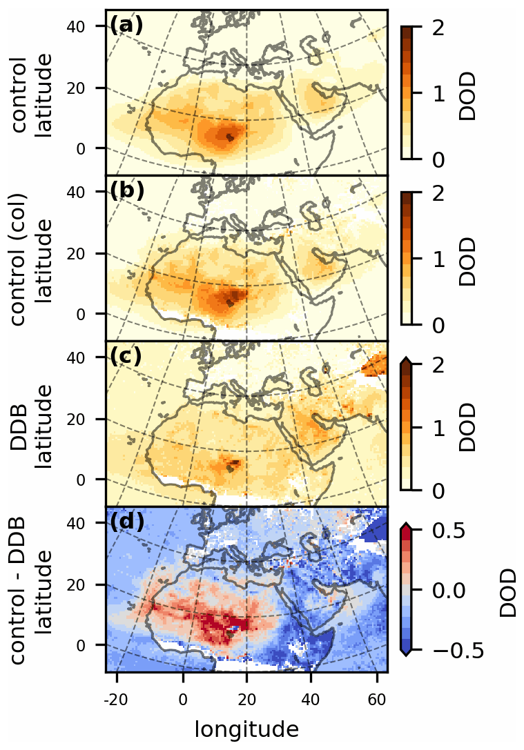
Figure 2 Averaged DOD from the control run and DDB during the whole study period. Panel (a) shows the average of the control run DOD. Panel (b) shows the average of the control run DOD in the pixels collocated with DDB. Panel (c) shows the average of the DDB DOD. Panel (d) shows the average difference between the control run and the DDB DOD.

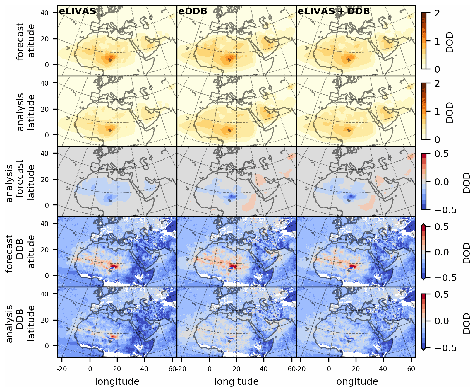
Figure 3 Averaged DOD from the experiments and differences with the DDB DOD during the whole study period. Experiments listed in Sect. 2.5 are represented in columns. The first and second rows show the average DOD for the forecast and analysis experiments respectively. The third row shows the difference between average analyses and forecasts. Collocated differences between the forecasts and the DDB DOD averages are shown in the fourth row. The last row shows the difference between the analyses and the DDB DOD averages.

Average maps of DOD are shown in Figs. 2 and 3. Compared to the DDB DOD, the control run shows a large overestimation of DOD over the Sahara and an underestimation elsewhere (Fig. 2). Figure 2 also shows relatively large values of DOD in the DDB panel over the North Atlantic that are not simulated in the control run. The first two rows of Fig. 3 show that the analyses have, in general, lower DOD values than the forecasts, which also have lower DOD values than the control experiment. The third row of Fig. 3 shows the average difference between forecasts and analyses. In this row, there is a common decrease in DOD values close to the Bodélé Depression after assimilation. Experiments eDDB and eLIVAS+DDB show increasing DOD in the eastern part of the domain in the analyses. Averaged differences of the simulations with respect to DDB are shown in the last two rows of Fig. 3. As expected, these differences are smaller in the eDDB and eLIVAS+DDB experiments because the DDB dataset is assimilated in these two experiments.

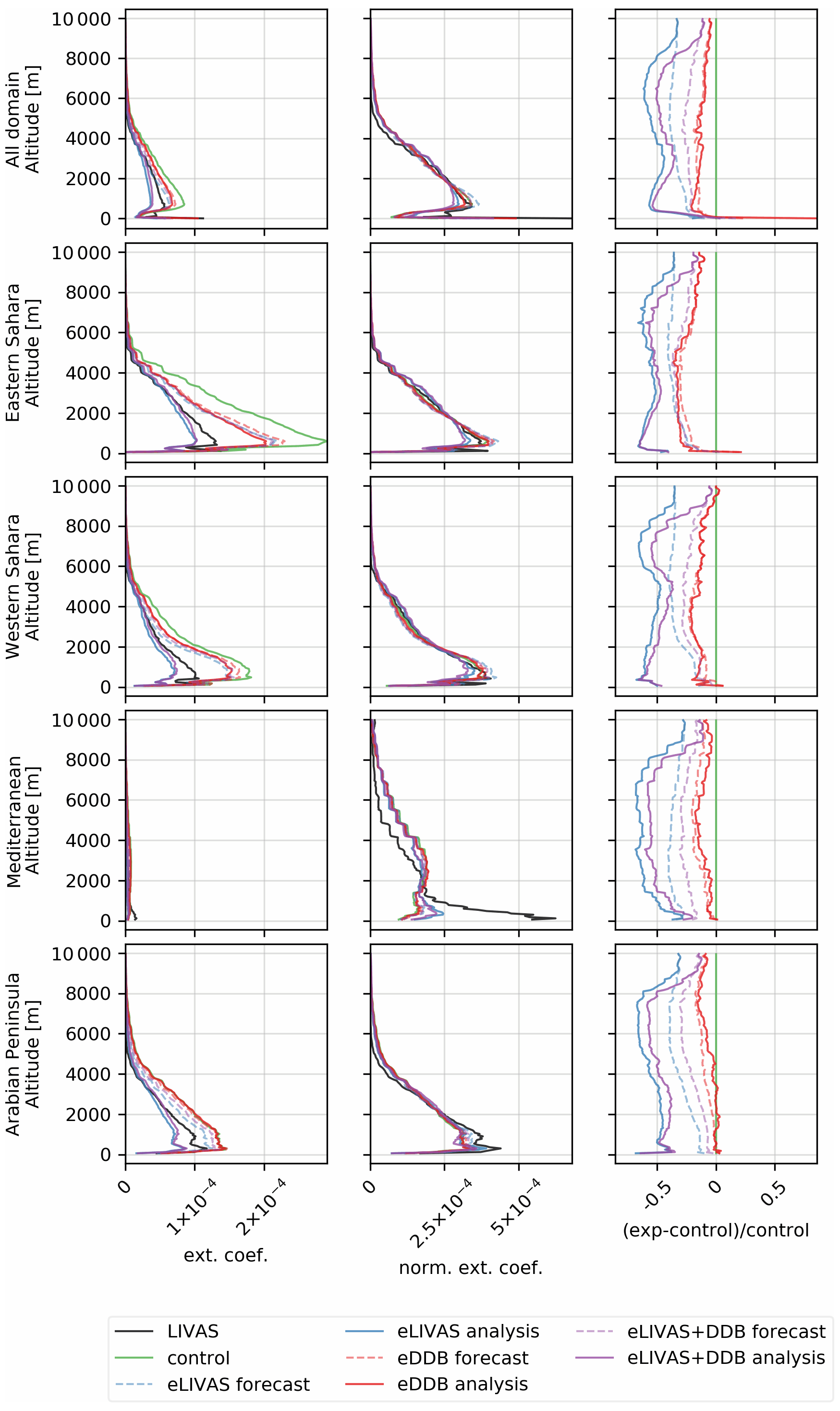
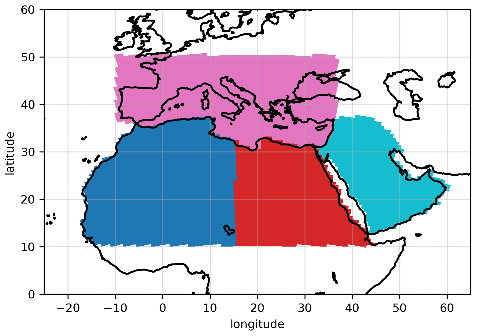
Figure 4 Collocated average dust extinction coefficients from model experiments and LIVAS-assimilated observations in the four-dimensional domain. The left column shows the mean extinction coefficient profiles in m⁻¹. The middle column shows the mean extinction profiles but normalized such that the vertical integration of each profile in the panel equals 1. The right column shows the relative difference between the mean value of each experiment and the control run. Each row represents a different geographical domain defined in Fig. B1, from top to bottom, as the full domain, Eastern Sahara, Western Sahara, the Mediterranean, and the Arabian Peninsula.

Figure 4 shows the average values of the assimilated LIVAS pure-dust extinction coefficient profiles compared with collocated model-derived dust extinction profiles for the full domain and the four regions presented in Fig. B1. The model systematically overestimates the dust extinction coefficient below 7 km in the analyses of experiments excluding LIVAS assimilation and in the forecasts, including experiments with LIVAS assimilation. In contrast, analyses with LIVAS assimilation underestimate the dust extinction coefficient below 7 km. The altitude of the maximum values and shape of the dust extinction coefficient are well captured by the model in all regions except the Mediterranean (middle column of Fig. 4), where the mean values are relatively small. Relative changes in the shape of the dust extinction coefficient compared to the control experiment are shown in the right column of Fig. 4. On average, experiments that assimilate LIVAS (i.e. eLIVAS, eLIVAS+DDB) show a stronger decrease in the extinction coefficient than eDDB. Analyses from eLIVAS and eLIVAS+DDB also show large decreases below 3 km of altitude over the Sahara and the Arabian Peninsula. The relative changes in the dust extinction coefficient of analyses and forecasts from eLIVAS and eLIVAS+DDB are larger above 3 km compared to eDDB. The different shapes of the forecasts and analyses from eLIVAS and eLIVAS+DDB (right column of Fig. 4) indicate that, close to the surface, the dust extinction profile is largely influenced by the model forward simulations (and the associated dust emissions) rather than by the assimilated information. In contrast, in the upper part of the atmosphere the assimilation of LIVAS data adds information to the analyses that is propagated in time by the subsequent forecast cycles. This effect is not as noticeable in eDDB. The relatively flat curves associated with eDDB show that the shape of the simulated dust vertical profile is mainly propagated from the forward model.

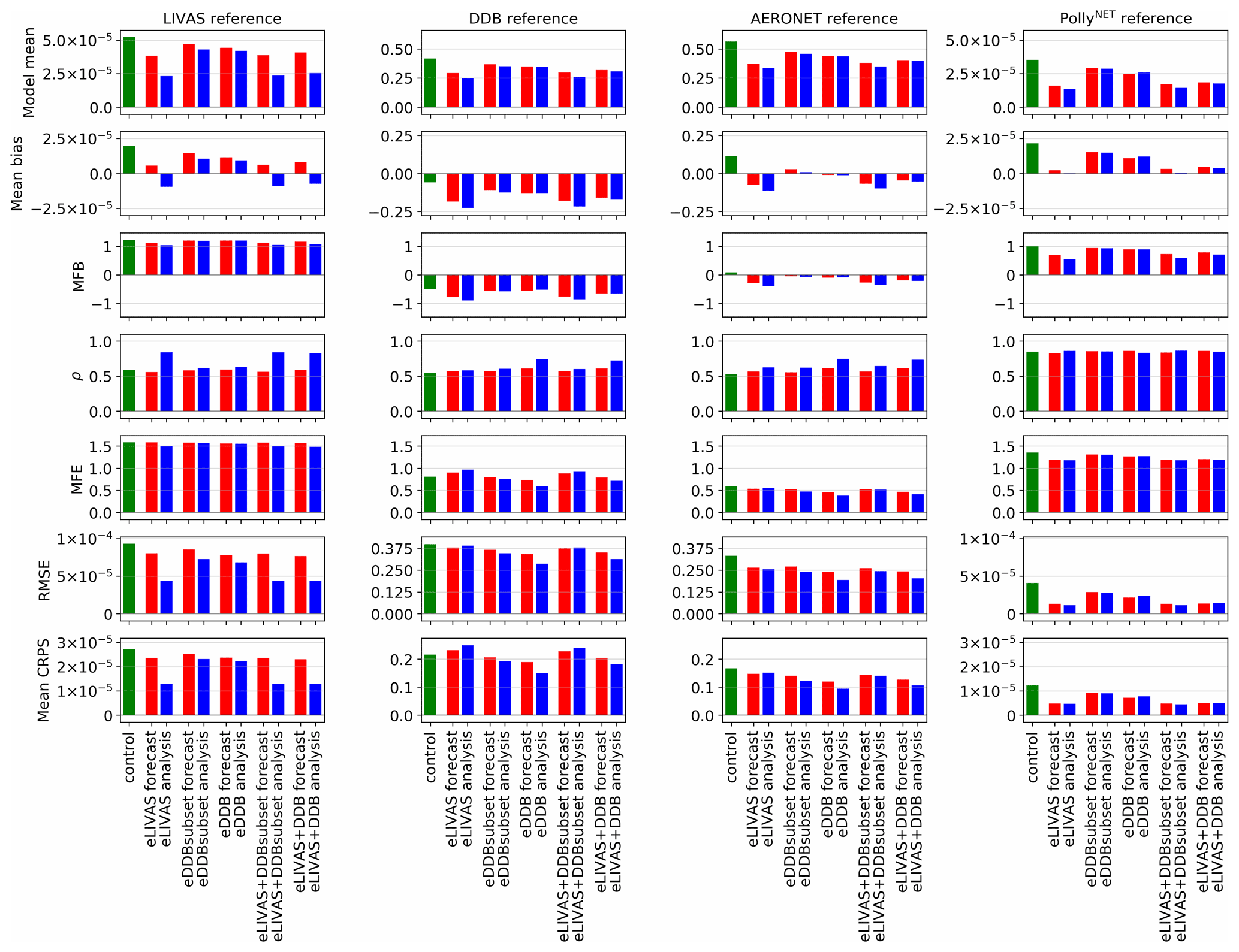
Figure 5 Verification scores against LIVAS dust extinction coefficient in the left column, scores against the DDB DOD dataset in the right column. Scores of the control run are shown in green, forecasts in red, and analyses in blue. In the left column, panels of model mean, mean bias, RMSE, and mean CRPS have units of m⁻¹.

The control run and the three selected assimilation experiments were also quantitatively evaluated against the LIVAS dust extinction coefficients and the DDB DOD using the scores described in Sect. 2. When evaluated against LIVAS (left column of Fig. 5), the control run shows a positive mean bias that decreases in the forecasts from all the assimilation experiments. When LIVAS is assimilated either with or without DDB, the analysis is negatively biased. The MFB is positive for all the experiments, and its absolute value slightly decreases with the assimilation. The negative mean bias of eLIVAS and eLIVAS+DDB analyses suggests that the assimilation tends to decrease rather than increase mass. Small mixing ratios have a smaller spread in the ensemble than the larger ones because the mass mixing ratio (the control vector in the DA) is bounded by zero. This may favour the decrease in mass for large DOD or extinction coefficient values but not for small values. Amending this behaviour could require, for example, application of non-linear transformations to the control vector and/or to the observation operator, which is beyond the scope of this work. As expected, the correlation coefficients obtained for the analyses from experiments assimilating LIVAS are significantly higher than those from the control run. However, the impact of the LIVAS assimilation is limited in the forecasts. Experiment eDDB slightly improves the correlation in the analyses but not in the forecasts. The MFE of analyses and forecasts is similar or smaller for the three assimilation experiments than for the control experiment. The RMSE and CRPS decrease similarly for all the forecasts. As expected, the RMSE and CRPS of eLIVAS and eLIVAS+DDB analyses show smaller values. It is also worth noting that the RMSE and CRPS of eDDB analyses decrease despite not assimilating LIVAS.

When evaluated against DDB DOD (right column of Fig. 5), the bias is negative for all experiments and products, and it is even becoming larger with assimilation. The opposite sign in the mean bias of the control run depending on the reference dataset suggests a potential inconsistency between DDB DOD and LIVAS. We note that none of the datasets has been bias-corrected. Inconsistencies may be related to the different quantities retrieved (DOD versus extinction coefficient), each one with its own uncertainties. By construction the DDB DOD (Sect. 2.1.2) may tend to be positively biased because although the selected scenes are mostly affected by dust, there will be always some contamination by other aerosols in the atmospheric column (see for example the relatively large DDB DOD values over the North Atlantic in Fig. 2). On the other hand, the low sensitivity of CALIOP to thin layers (Kar et al., 2018) or the signal attenuation in CALIOP measurements when the dust load is large could also play a role in the obtained biases. When comparing with DDB DOD, the correlation coefficient is larger for both forecasts and analyses when DDB is assimilated (eDDB and eLIVAS+DDB), while the improvement of this score is smaller for eLIVAS. The analyses show a better correlation coefficient with respect to DDB than the forecasts, and both show a better behaviour than the control run for all the experiments. The three error scores (MFE, RMSE, and CRPS) differ across two distinct groups of experiments. These errors increase in eLIVAS for both the forecast and analyses with respect to the control run. In contrast, the other two experiments (eDDB and eLIVAS+DDB) show a decrease in these error scores for both the forecasts and analyses. The latter is expected as the scores are computed taking the DDB as the reference.

In summary, the results of the cross-comparison checks are consistent with the assimilated observations used in each experiment. Also, when LIVAS is used as the reference dataset, all experiments improve their scores after assimilation for both forecasts and analyses. The comparison shows mixed results when the reference dataset is DDB.

Figure 6 Verification scores against DOD filtered from AERONET AOD observations.

3.2 Evaluation against ground-based measurements

Figure 6 presents the scores for each experiment when evaluated against dust-filtered AOD at 550 nm from AERONET stations (Appendix A). We acknowledge that the filter used for creating this AERONET DOD dataset (Ångström exponent less than 0.3) can bias our analysis towards large values of DOD. The left column of Fig. 6 shows the scores when all the filtered observations are taken into account (2681 observations), while the other three columns show the scores in northern Africa (1394 observations), the Mediterranean and southern Europe (1029 observations), and the Middle East (258 observations). The list of stations used for each set of scores is given in Appendix A, and it is based on the list of stations used for operational verification of the SDS-WAS forecasts.

The bias of the control run is positive, which contrasts with the negative bias resulting from the comparison with DDB (Fig. 5). While the different spatial and temporal localizations used in the comparison may play an important role in this difference, an additional explanation is that the dust filter in the DDB dataset is less conservative and provides on average larger DOD values due at least partly to the presence of other aerosols. The high positive bias of the control run for all AERONET stations decreases in absolute terms in all the experiments after assimilation, consistent with the systematic decrease in the simulated DOD shown in the first row of Fig. 5. Forecast and analyses from experiments where LIVAS was assimilated (eLIVAS and eLIVAS+DDB) show a stronger negative bias and MFB than eDDB, notably in the Mediterranean and southern European (a subset of 39 % of all the AERONET observations used here) and Middle Eastern panels (9 % of all the AERONET observations used here).

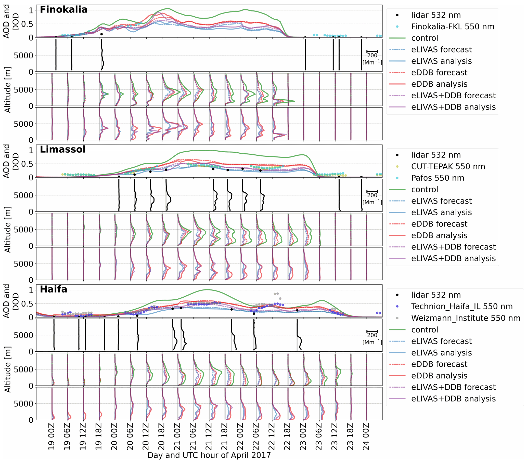
Figure 7 Simulated and measured dust extinction coefficient during the CyCARE and Pre-TECT campaigns by PollyNET lidars. The figure contains three groups (for the three measurement sites) with four panels each. The first panel of each group shows the DOD evolution estimated from the lidar measurements (black dots, equal to the vertical integration of the dust extinction coefficient profiles), the AOD without dust filtering for the AERONET station (coloured dots), the DOD of the control experiment (green line), the DOD from the forecasts (dashed lines), and analyses (continuous lines) for the three selected assimilation experiments. The second row of each group shows the vertical profiles of the measured dust extinction coefficient. The third row of each group shows the dust extinction coefficient from the control run (in green) and the forecasts (dashed lines). The fourth row of each group shows the dust extinction coefficient from the analyses. The scale for all the dust extinction coefficient profiles is shown on the right-hand side of the second panel in each group.

The correlation coefficient increases in all the assimilation experiments compared with the control for northern Africa and the Mediterranean, particularly in the analyses but also in the forecasts. Experiment eDDB shows higher correlations. Over the Middle East, with only 258 observations, the correlation coefficient is very low but still positive. Over northern Africa, all the experiments show smaller errors (MFE, RMSE, CRPS) in comparison with the control run. With the exception of eLIVAS, all the analyses have smaller errors than the forecasts and – similarly to the correlation coefficient – the experiments where DDB DOD was assimilated show better scores in their analyses.

As introduced in Sect. 2, we used lidar retrievals of pure-dust profiles for the evaluation of the experiments. The evaluation was conducted for the dust event above the eastern Mediterranean between 19 and 24 April 2017, whose extent and dynamics can be observed in the right column of Fig. 1.

We compared our five experiments with the dust extinction coefficient provided by these lidars. Figure 7 shows the comparison between the lidar measurement in the three sites, the control run, the forecasts and analyses from three experiments (eLIVAS, eDDB, eLIVAS+DDB), and the AOD from AERONET sites close to the lidar instruments, without filtering by Ångström exponent. Rows 1, 5, and 9 of Fig. 7 show the integrated dust extinction coefficient for lidar measurements and model runs and the AOD from AERONET instruments close to these sites. The control run is overestimated in the three sites, and both analyses and forecast show values closer to the AERONET AOD and the lidar-integrated DOD. The three experiments capture the timing and the magnitude of the dust event. Qualitatively, eDDB overestimates the AOD and lidar-integrated measurements, eLIVAS+DDB is closer to AERONET AOD measurements, and eLIVAS is closer to the lidar-integrated DOD. The control run not only overestimates the dust profile, but also underestimates the height of the maximum values in the plume (e.g. in the Limassol panel, 21 and 22 April). For forecasts and analyses, the experiments where LIVAS was assimilated (eLIVAS and eLIVAS+DDB) are able to decrease the dust concentration in the lower layers (below 2.5 km), making the shape of the profiles similar to the observed ones. The eDDB profiles do not show this feature.

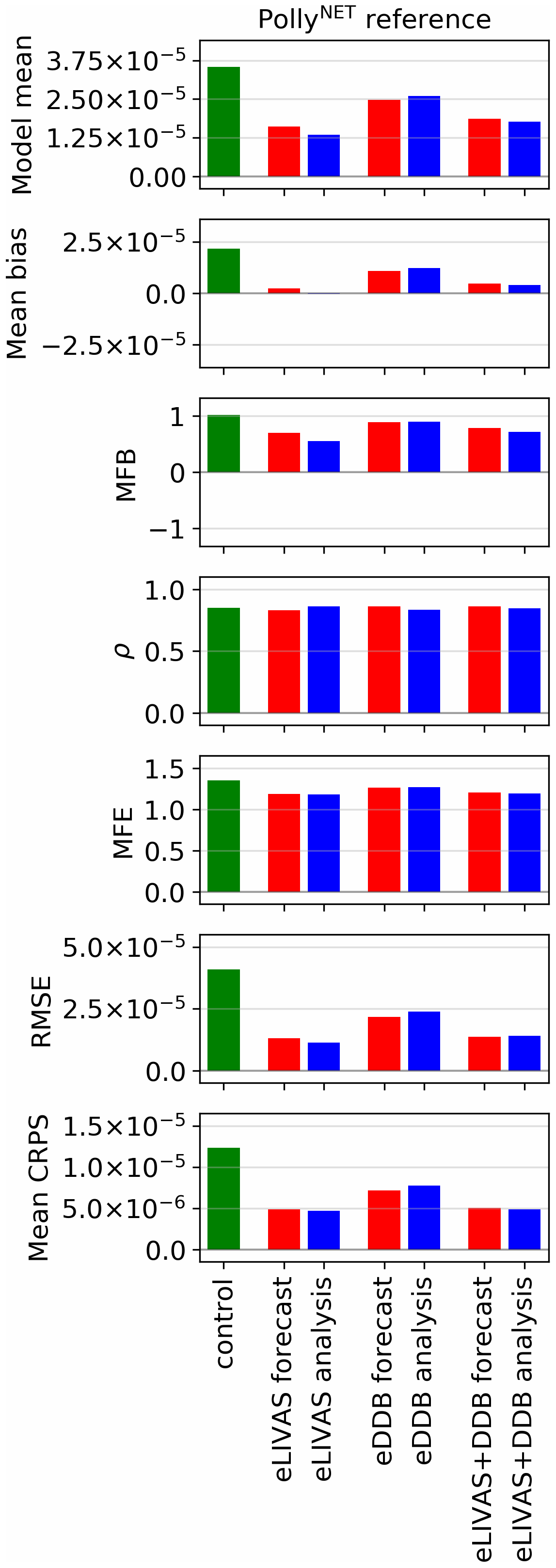
Figure 8 Verification scores against ground-based PollyNET lidar dust extinction coefficients from the CyCARE and Pre-TECT campaigns. Panels of model mean, mean bias, RMSE, and mean CRPS have units of m⁻¹.

The overall quantitative evaluation is shown in Fig. 8. These scores have been computed by concatenating all the pairs of observed and simulated extinction coefficients in a vector without distinguishing among profiles on the computation. In general terms, both bias scores are smaller for eLIVAS and eLIVAS+DDB than for eDDB. The correlation coefficient is weakly affected by the assimilation in all experiments and the MFE is slightly smaller for experiments where LIVAS was assimilated. RMSE and CRPS behave similarly, with improvement for all the experiments compared to the control run, particularly for those where LIVAS was assimilated.

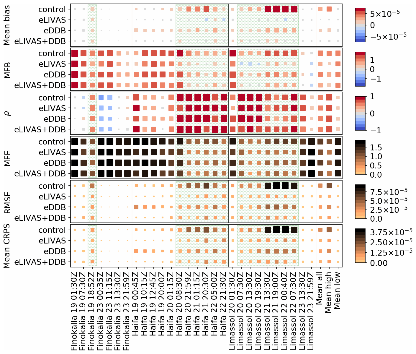
Figure 9 Verification scores of the model analyses for the dust extinction coefficient profiles against measurements of PollyNET lidars of Fig. 7. Mean bias, RMSE, and CRPS have units of m⁻¹. Profiles with high values of extinction are shown with a green shade. The last three columns show averages of the scores for the non-shaded profiles (mean low), for the shaded profiles (mean high), and for all profiles (mean all). The areas of the squares are proportional to their values (in colours).

We have also computed the evaluation scores for each of the available profiles (Fig. 7), which are summarized in Fig. 9. The assimilation performance was split into two groups. The first group is characterized by low values of measured dust extinction coefficient (non-shaded columns in Fig. 9), where the dust plume cannot be easily identified in Fig. 7. A second group of profiles corresponds to high dust extinction coefficients (green-shaded columns in Fig. 9). For these profiles, it is possible to visually identify in Fig. 7 the altitude and shape of the dust plume. We have averaged these scores of individual profiles in the last three columns of Fig. 9. In Fig. 9, the mean all column shows the average of the scores of all the profiles, the mean high column shows the average of the scores of the profiles with strong dust extinction coefficients (i.e. green-shaded columns of this figure), and the mean low column shows the average of the scores of the profiles with small values of measured dust extinction coefficients (non-shaded columns in Fig. 9). These last three columns in Fig. 9 are also shown in Table 2. We note that scores of Fig. 8 and the last three columns of Fig. 9 are computed differently. In the former, we have concatenated all the profiles and computed the scores, while in the latter, we have computed the scores for individual profiles and then averaged their values. This methodological difference impacts, for example, the values of the correlation coefficient and RMSE when comparing the mean all values of Table 2 with those of Fig. 8.

For the group of profiles with small values of the dust extinction coefficient (“mean low” in Fig. 9), the absolute scores (mean bias, RMSE, and CRPS) are small because simulated and observed values are also small, but they do not improve after the assimilation. Similarly, the normalized scores (MFE and MFB) and the correlation coefficient do not improve. The group of profiles with high dust extinction coefficients (green-shaded columns in Fig. 9) generally show better normalized scores than the group with low dust values. With the exception of the correlation coefficient, all the scores in this group improved after assimilation. In this mean high group the mean bias drastically decreased when LIVAS was assimilated (eLIVAS and eLIVAS+DDB). Similarly, MFB, MFE, RMSE, and CRPS improved with LIVAS assimilation. The correlation coefficient does not improve with assimilation, but the degradation of this score in all experiments with respect to the control run remains below 5 % of the control run value. Overall, when dust extinction is large, all analyses improved in all scores, with the exception of the correlation coefficient. While improvements are enhanced when LIVAS is assimilated, they are still non-negligible for eDDB. All in all, despite the sparse spatial coverage of LIVAS compared to DDB, this evaluation shows that dust extinction profiles are best constrained in experiments where LIVAS is assimilated.

Table 2 Values of the last three columns of Fig. 9.

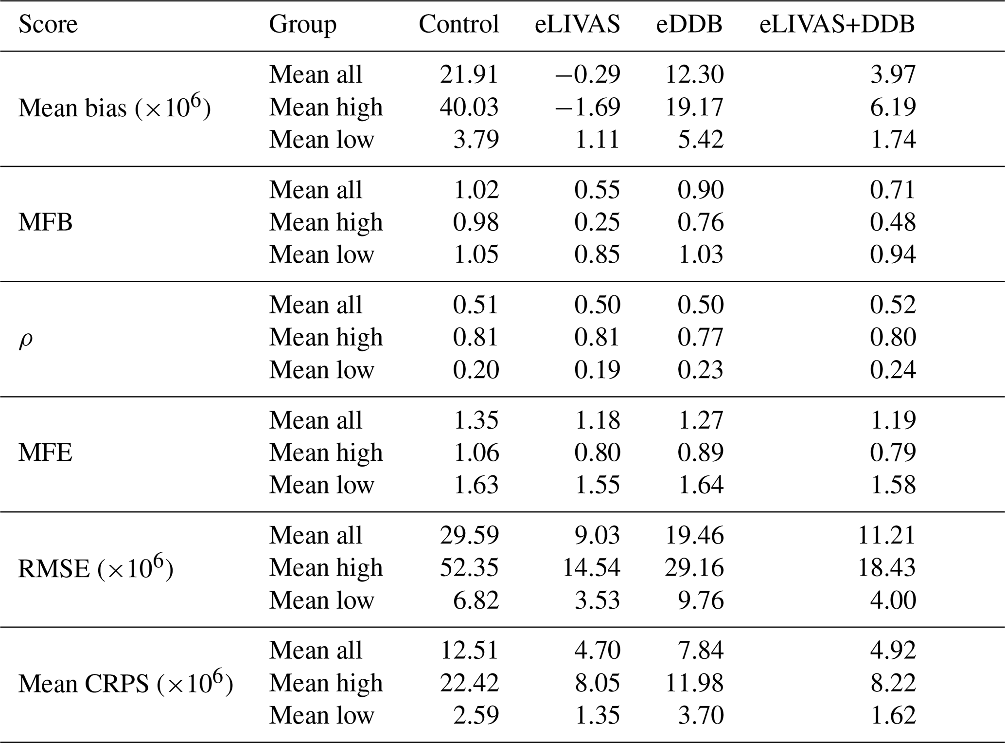
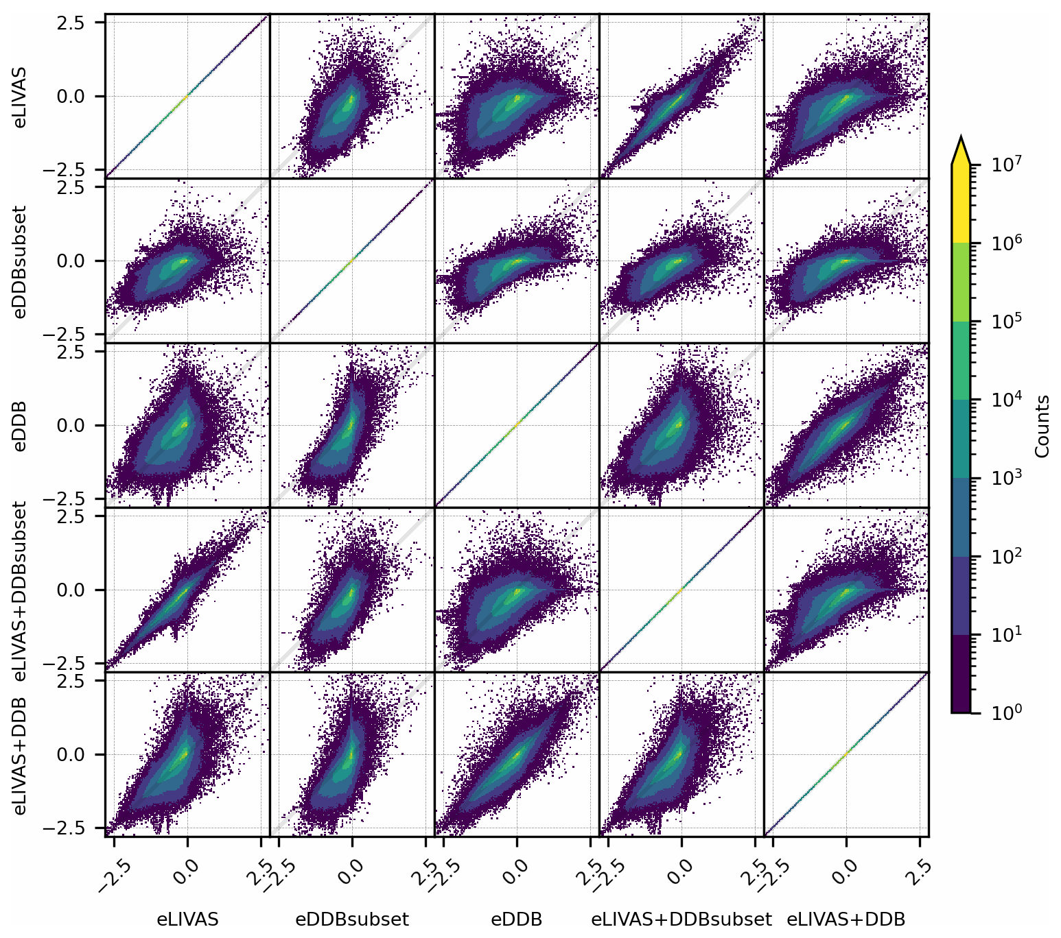
Figure 10 Bi-dimensional histograms of the difference between analyses and the control run DOD. Transposed plots in the figure are symmetrical with respect to the 1:1 line. Colour scale shows the counts of analysis minus control in a box of ΔDOD=0.37, that is, 151 bins between −2.8 and 2.8. Please note the logarithmic scale of the counts.

3.3 Consistency between column and profile assimilation and the role of a narrow satellite footprint

Along with the eDBB, eLIVAS, and eLIVAS+DDB experiments shown in the previous sections, we have performed the same analyses with the DDBsubset dataset, namely eDDBsubset and eLIVAS+DDBsubset. We recall from Sect. 2.1.2 that DBBsubset contains the DBB DOD, but only when it is collocated with LIVAS. We use here this dataset for studying the impact of assimilating vertically resolved dust observations along with the impact of the different fields of view of the measurements upon our analyses.

We have included the verification scores in Fig. C1. This figure is equivalent to Figs. 5, 6, and 8 but with the addition of eDDBsubset and eLIVAS+DDBsubset experiments. Figure C1 shows that, as expected, the skill scores of eDDBsubset are qualitatively analogous to those of eDDB, but the magnitude of the change with respect to the control is smaller. The better scores of eDBB over eDDBsubset underline the importance of the horizontal coverage of the observations in our assimilation. Similarly, eLIVAS+DDBsubset reaches scores close to those of eLIVAS. This indicates that the impact of the LIVAS-assimilated observations is more important than that of DDBsubset in the eLIVAS+eDDBsubset scores.

More interesting is the comparison of eLIVAS and eDDBsubset in Fig. C1. They have a similar horizontal coverage and eLIVAS performed better than eDDBsubset when evaluating against the vertical profiles of PollyNET. However, the eLIVAS scores are worse than those of eDDBsubset for the comparisons with DBB DOD and some (but not all) of the scores in the AERONET DOD panel of Fig. C1. We argue that a direct comparison among experiment analyses can further help elucidate the differences in the performance between the two experiments.

Although DDBsubset was designed to have a similar horizontal and temporal coverage to LIVAS, a direct comparison between the eDDBsubset and eLIVAS experiments should also take into account that (i) LIVAS provides direct observational information in the vertical coordinate, while DDBsubset does not, (ii) the vertical influence of LIVAS information is only partial if the column is not complete, in contrast to the DDB DOD that is propagated to the whole column, and (iii) DDB only provides data during the afternoon overpass (about 13:30 LT), while LIVAS provides data during afternoon and night overpasses. Nighttime profiles have better quality, and given the assimilation cycle design and the temporal localization applied, they should influence the 00:00 UTC analyses more than the afternoon overpasses, with more impact over the forecast and subsequent analyses.

It is possible to compare the experiments by inspecting the histograms of differences between the analyses and the control run. We have computed these differences for DOD in Fig. 10 and for dust extinction coefficient in Fig. 11. Figure 10 shows bi-dimensional histograms of the DOD differences for the five experiments. The 1:1 line indicates that the respective analyses produce the same differences with the control run, i.e. they are equal. Points in quadrants I and III indicate that both experiments increase and decrease the DOD values at the same locations and times, which is a sign of consistency. It can be seen that the (eDDB, eLIVAS+DDB) panel shows less deviation with respect to the 1:1 line than the (eLIVAS, eLIVAS+DDB) case. This indicates that most of the impact of the observations in the eLIVAS+DDB experiments comes from DDB rather than from LIVAS, which is consistent with the scores presented in previous sections. A similar result is found when comparing (eLIVAS+DDBsubset, eLIVAS) with (eLIVAS+DDBsubset, eDDBsubset). In this case, eLIVAS+DDBsubset is closer to eLIVAS than eDDBsubset. Because the datasets have a similar horizontal coverage, we conclude that either LIVAS adds more information to the analyses than the DOD from DDBsubset or that the nighttime overpass of CALIOP has a stronger influence on the 00:00 UTC analyses, which is also propagated to the forecasts. Similarities between (eLIVAS+DDB, eLIVAS) and (eLIVAS+DDB, eDDBsubset) suggest that the LIVAS assimilation is less important than the DDB assimilation in the eLIVAS+DDB case because of the smaller observational coverage. A relatively large spread can be noticed in the (eLIVAS, eDDB) panel and to a lesser extent in the (eLIVAS, eDDBsubset) panel.

The spread in the (eDDBsubset, eDDB) panel is associated with the smaller coverage of DDBsubset. In this panel, most values lie around zero on the eDDBsubset axis, which is directly related to the reduced amount of assimilated data. A small number of values (around the 6 % of this panel) are in quadrants II and IV, meaning that the increments with respect to the control DOD of the eDDBsubset and eDDB analyses are of different signs. A possible explanation is a potentially poor estimation of the terms outside the diagonal of the background error covariance matrix, as they should spread consistently (or at least in the same direction) the DDBsubset observational influence to the remaining pixels covered by the full DDB dataset.

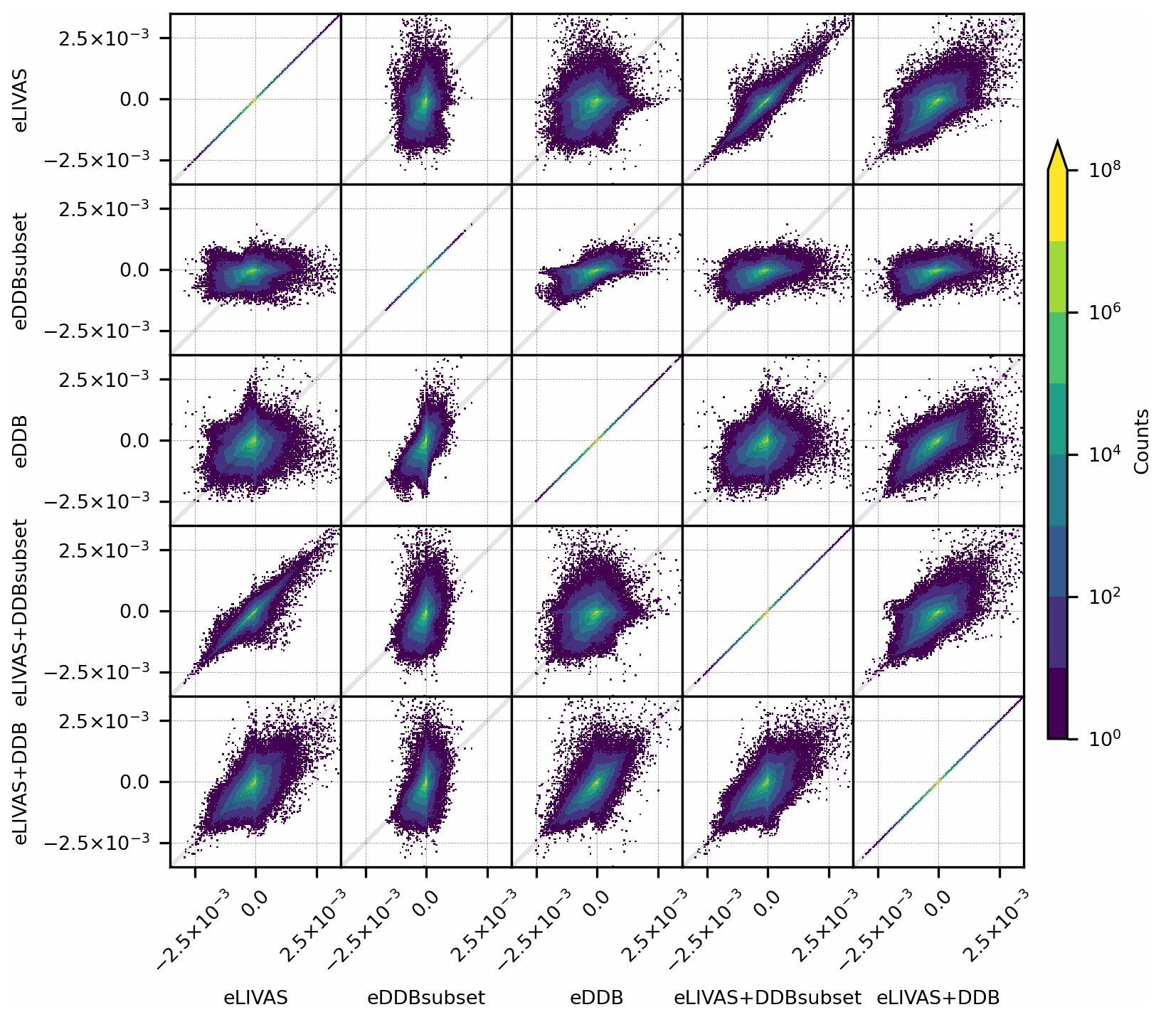
Figure 11 Similar to Fig. 10 but for the dust extinction coefficient. The width of the bins is $\mathrm{4.63}\times {\mathrm{10}}^{-\mathrm{5}}$ m⁻¹.

Bi-dimensional histograms of the differences in dust extinction coefficient between analyses and the control run experiment are shown in Fig. 11. In general terms, this figure shows similar but less clear features than the DOD in Fig. 10. Notable differences are in the row comparing eDDBsubset with the other experiments, where the values in the panels do not show the clear correlation that appears in the DOD case. This indicates that the shapes of the dust profiles in the experiments assimilating LIVAS substantially differ from those assimilating DDB. This is also supported by the eLIVAS+DDB panels, where the larger influence of DDB on LIVAS observations shown for DOD in Fig. 10 is less clear for the extinction coefficient. As we show in Sect. 3.2, the assimilation of LIVAS data (either in eLIVAS or eLIVAS+DDB) can produce more accurate dust profiles. This demonstrates that the assimilation of vertically resolved pure-dust extinction coefficients can effectively improve the dust vertical distribution in forecasts and analyses.

4 Conclusions

We performed, analysed, and evaluated model experiments assimilating spaceborne dust extinction coefficient profiles and DOD over a 2-month period over northern Africa, the Middle East, and Europe. We filtered the AOD observations from VIIRS DB to obtain a DOD dataset, and we have used for the first time the CALIPSO-based LIVAS pure-dust dataset in a data assimilation framework. In most cases, the assimilation of these products (and their combination) is beneficial for analyses and forecasts.

Experiments that assimilate DDB yield better DOD error scores than those that assimilate only LIVAS when evaluated against AERONET. However, the assimilation of only LIVAS can still achieve significant improvements in these DOD scores.

We evaluated the potential improvements in the representation of the dust vertical profile using a handful of high-quality ground-based lidar pure-dust extinction coefficient measurements performed during the CyCARE and Pre-TECT experimental campaigns in the Mediterranean. The assimilation of LIVAS leads to a better representation of the dust extinction coefficient profiles than the assimilation of DDB alone. Jointly assimilating DDB and LIVAS yields the second-best scores for both the DOD and the dust extinction coefficient profile, which proves their suitability for dust forecast applications.

We have also focused on the limitations of the narrow footprint of LIVAS compared with the large swath of DDB, which reduces the observational influence on the analyses. However, the impact of the vertically resolved information provided by LIVAS is significant, and with a similar coverage it produces an even larger impact on the analyses than the assimilation of DOD.

Our findings strongly support the conclusions of Cheng et al. (2019) in that the assimilation of aerosol profiles can improve their vertical representation in models. We additionally show that the vertical profiles of dust extinction coefficient can be constrained by assimilating the LIVAS product. We are aware of the limitations of this study due to the limited availability of ground-based PollyXT lidar measurements. We are looking forward to the publication of ground-based pure-dust lidar datasets from version 3 of the NASA Micro-Pulse Lidar Network (MPLNET) and EARLINET that would be very useful for a long-term assimilation and evaluation of simulated dust extinction profiles from model forecasts and analyses. Our work shows the value of spaceborne polarization lidars for improving desert dust forecasts and analyses. As such, future satellite missions with combined extinction and depolarization capability, such as the Earth Cloud Aerosol and Radiation Explorer (EarthCARE), are expected to further contribute not only to desert dust research, but also to operational forecasts if real-time products are made available.

Appendix A: AERONET sites

List of AERONET sites used in Sect. 3.2. The value in parentheses indicate the number of observations used for each station.

Mediterranean (1029). AgiaMarina_Xyliatou (2), Aras_de_los_Olmos (7), Badajoz (11), Barcelona (4), Ben_Salem (27), CUT-TEPAK (49), Cabo_da_Roca (55), Cairo_EMA_2 (70), Carpentras (5), Coruna (15), Eforie (2), Eilat (121), El_Arenosillo (45), Ersa (5), Evora (29), FORTH_CRETE (12), Finokalia-FKL (19), Galata_Platform (4), Gloria (2), Gozo (19), Granada (34), IMAA_Potenza (1), IMS-METU-ERDEMLI (29), LAQUILA_Coppito (1), Lamezia_Terme (24), Lampedusa (17), Lecce_University (20), Madrid (4), Medenine-IRA (84), Messina (4), Modena (1), Montsec (2), Murcia (7), Napoli_CeSMA (4), OHP_OBSERVATOIRE (5), Palencia (3), Palma_de_Mallorca (11), Rome_Tor_Vergata (9), SEDE_BOKER (99), Tabernas_PSA-DLR (41), Technion_Haifa_IL (49), Tizi_Ouzou (10), Toulon (2), Toulouse_MF (2), Weizmann_Institute (61), Zaragoza (2).

Northern Africa (1394). Banizoumbou (123), Capo_Verde (106), Dakar (349), El_Farafra (95), IER_Cinzana (163), Ilorin (47), LAMTO-STATION (50), Saada (80), Santa_Cruz_Tenerife (124), Tamanrasset_INM (257).

Middle East (258). IASBS (17), KAUST_Campus (97), Masdar_Institute (70), Mezaira (74).

Appendix B: Regions for LIVAS collocation

We present in Fig. B1 the definition of regions used in Fig. 4.

Figure B1 Definition of regions of Fig. 4. The Mediterranean region is shown in pink, Western Sahara in blue, Eastern Sahara in red, and Arabian Peninsula in cyan.

Appendix C: Scores of eDDBsubset and eLIVAS+DDBsubset

We present in Fig. C1 the scores for the five experiments listed in Sect. 2.5.

Figure C1 Scores of the full set of five experiments. Similar to Figs. 5, 6, and 8 but with the addition of eDDBsubset and eLIVAS+DDBsubset.