Direct measurements of ozone response to emissions perturbations in California

A new technique was used to directly measure O₃ response to changes in precursor NO_x and volatile organic compound (VOC) concentrations in the atmosphere using three identical Teflon smog chambers equipped with UV lights. One chamber served as the baseline measurement for O₃ formation, one chamber added NO_x, and one chamber added surrogate VOCs (ethylene, m-xylene, n-hexane). Comparing the O₃ formation between chambers over a 3-hour UV cycle provides a direct measurement of O₃ sensitivity to precursor concentrations. Measurements made with this system at Sacramento, California, between April–December 2020 revealed that the atmospheric chemical regime followed a seasonal cycle. O₃ formation was VOC-limited (NO_x-rich) during the early spring, transitioned to NO_x-limited during the summer due to increased concentrations of ambient VOCs with high O₃ formation potential, and then returned to VOC-limited (NO_x-rich) during the fall season as the concentrations of ambient VOCs decreased and NO_x increased. This seasonal pattern of O₃ sensitivity is consistent with the cycle of biogenic emissions in California. The direct chamber O₃ sensitivity measurements matched semi-direct measurements of $\mathrm{HCHO}/{\mathrm{NO}}_{\mathrm{2}}$ ratios from the TROPOspheric Monitoring Instrument (TROPOMI) aboard the Sentinel-5 Precursor (Sentinel-5P) satellite. Furthermore, the satellite observations showed that the same seasonal cycle in O₃ sensitivity occurred over most of the entire state of California, with only the urban cores of the very large cities remaining VOC-limited across all seasons. The O₃-nonattainment days (MDA8 O₃>70 ppb) have O₃ sensitivity in the NO_x-limited regime, suggesting that a NO_x emissions control strategy would be most effective at reducing these peak O₃ concentrations. In contrast, a large portion of the days with MDA8 O₃ concentrations below 55 ppb were in the VOC-limited regime, suggesting that an emissions control strategy focusing on NO_x reduction would increase O₃ concentrations. This challenging situation suggests that emissions control programs that focus on NO_x reductions will immediately lower peak O₃ concentrations but slightly increase intermediate O₃ concentrations until NO_x levels fall far enough to re-enter the NO_x-limited regime. The spatial pattern of increasing and decreasing O₃ concentrations in response to a NO_x emissions control strategy should be carefully mapped in order to fully understand the public health implications.

1 Introduction

Ground-level ozone (O₃) is an oxidant that inflames airways and damages tissue in the respiratory tract, leading to increased coughing, wheezing, shortness of breath, and other asthmatic symptoms (US EPA, 2020b). Maximum daily average 8 h (MDA8) O₃ concentrations designed to protect public health are codified in the National Ambient Air Quality Standards (NAAQS) (US EPA, 2021) and the California Ambient Air Quality Standards (CAAQS) (California Air Resources Board, 2007). Seven of the 10 cities across the United States with the highest O₃ concentrations are located in California (American Lung Association, 2020), making O₃ pollution a continued public health threat for millions of California residents more than four decades after O₃ abatement efforts began.

O₃ levels are often described by the maximum daily average 8 h concentration. The annual fourth-highest MDA8 O₃ concentration averaged over 3 years has special regulatory significance. This design value determines whether the region containing the monitor complies with the O₃ NAAQS. O₃ design values in California decreased steadily between the years 1980 and 2019 (Fig. 1) due to the success of emissions control programs that reduced concentrations of precursors broadly divided into two groups: oxides of nitrogen (NO_x) and volatile organic compounds (VOCs) (Parrish et al., 2016; Simon et al., 2015). Continued progress after the year 2010 has been slower, and O₃ design values even increased in some air basins between the years 2015–2018 (Fig. 1). Multiple factors have been proposed to explain the lack of further reductions in O₃ concentrations in recent years. These potential factors include (i) growing importance of precursor VOC emissions not previously accounted for in the planning process as major sources such as transportation have been controlled (McDonald et al., 2018; Shah et al., 2020), (ii) an imbalance in the historical degree of NO_x and VOC reductions (Cox et al., 2013; Parrish et al., 2016; Pollack et al., 2013a; Steiner et al., 2006), or (iii) more frequent heat waves (Jacob and Winner, 2009; Jing et al., 2017; Pusede et al., 2015; Rasmussen et al., 2013; Weaver et al., 2009) and wildfires (Jaffe et al., 2013; Lindaas et al., 2017; Lu et al., 2016; Singh et al., 2012) as a consequence of climate change. All these theories are supported to varying degrees by indirect measurements or model predictions, but there is an absence of strong direct evidence that identifies dominant factors contributing to the increased O₃ concentrations. The uncertainty that lingers over the recent O₃ trends suggests that fresh approaches are needed to directly verify the optimum emissions control path.

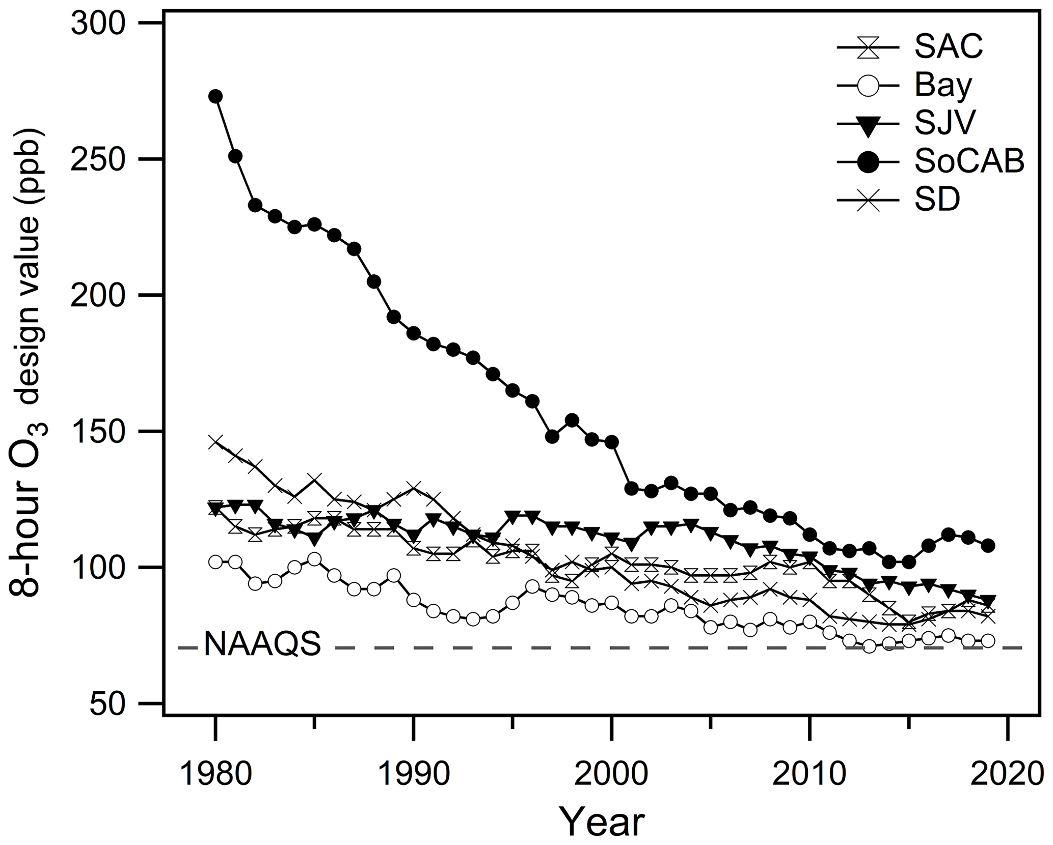
Figure 1 The 8 h O₃ design value in five air basins in California from 1980 to 2019. The dash line is the 2015 8 h O₃ NAAQS (=70 ppb). The five air basins include the Sacramento Valley (SAC), San Francisco Bay Area (Bay), San Joaquin Valley (SJV), South Coast Air Basin (SoCAB), and San Diego County (SD). Data collected from the California Air Resources Board (https://www.arb.ca.gov/adam, last access: 9 June 2021).

O₃ formation has been studied for decades in California, using both measurements and model simulations (Kroll et al., 2020). These past studies provide important background information about the effects of precursor NO_x and VOC species and help build the foundation for new studies. Statistical analyses of long-term surface measurements have determined that lower NO_x concentrations are associated with higher O₃ concentrations on weekends (Pollack et al., 2012; Pusede and Cohen, 2012) and higher temperatures are associated with increased VOC emissions and chemical reaction rates, leading to higher O₃ concentrations during warm stagnation events (Lafranchi et al., 2011; Nussbaumer and Cohen, 2020). These long-term studies suggest that VOCs are the limiting precursor for O₃ formation in the center of large cities, while NO_x is the limiting precursor in downwind areas (Lafranchi et al., 2011; Pusede and Cohen, 2012). Neither long-term analysis method clearly explains the recent trend of increasing O₃ concentrations in Los Angeles.

O₃ sensitivity has also been analyzed over shorter timescales using ratios of photochemical indicator species including ${\mathrm{H}}_{\mathrm{2}}{\mathrm{O}}_{\mathrm{2}}/{\mathrm{HNO}}_{\mathrm{3}}$ and $\mathrm{HCHO}/{\mathrm{NO}}_{\mathrm{2}}$ (Sillman, 1995; Tonnesen and Dennis, 2000). Satellite retrievals of $\mathrm{HCHO}/{\mathrm{NO}}_{\mathrm{2}}$ from the Global Ozone Monitoring Experiment (GOME), the SCanning Imaging Absorption spectroMeter for Atmospheric CHartograpHY (SCIAMACHY), the Ozone Monitoring Instrument (OMI), and the TROPOspheric Monitoring Instrument (TROPOMI) have extended these O₃ sensitivity calculations over broad geographical regions (Chossière et al., 2021; Duncan et al., 2010; Jin et al., 2017; Martin et al., 2004; Schroeder et al., 2017a). The short-term measurements generally support the findings from the long-term studies but once again fail to identify the dominant factor(s) driving the recent increase in O₃ design values. Reactive chemical transport models (CTMs) have been used extensively to predict the effectiveness of candidate emissions control programs (Brown, 2018; California Air Resources Board, 2018; Meng et al., 1997; Sillman, 1999), and so one might expect that they would provide the most detailed explanation for recent O₃ trends. Models are necessarily incomplete approximations to highly complex real-world systems, and so they are often incapable of predicting subtle features in pollutant trends. No model calculation has been able to reproduce the observed increase in O₃ design values (Parrish et al., 2017). It is unclear whether this failure stems from a lack of accurate emissions trends, an incomplete description of atmospheric chemistry, or an incomplete representation of the effects of shifting climate on O₃ formation mechanisms.

Recent advances in measurement techniques provide new tools to study O₃ sensitivity directly. Mobile smog chambers bridge the gap between laboratory studies and the real atmosphere. Past studies have designed mobile smog chambers to measure the aging of secondary pollutants (i.e., O₃, SOA) from certain emission sources (Howard et al., 2008, 2010b; Li et al., 2019; Platt et al., 2013; Presto et al., 2011). It is difficult to evaluate sensitivity of secondary pollutants formed from multiple sources using a single smog chamber. Recently, a mobile dual-smog-chamber system has been used to directly measure the SOA formation in ambient air (Jorga et al., 2020; Kaltsonoudis et al., 2019). The design used in the current study consists of three chambers that can simultaneously measure the non-linear response of O₃ formation to NO_x and VOC perturbations. The automated valve and sampling incorporated into this design also allows long-term remote field measurements to evaluate the seasonal trends in O₃ sensitivity. At the same time, the satellite TROPOMI launched by the European Space Agency (ESA) in October 2017 provides measurements of HCHO and NO₂ tropospheric vertical column densities (TVCDs) with 3.5 km × 5.5 km spatial resolution that can start to resolve O₃ perturbations around major sources such as wildfires (Ialongo et al., 2020; Veefkind et al., 2012; Vigouroux et al., 2020b). The purpose of this study is to combine these two new measurement techniques into a detailed analysis of O₃ sensitivity to precursor NO_x and VOC emissions spanning an entire spring–summer–fall cycle in California. Daily measurements from smog chamber perturbation experiments are analyzed for short-term trends (day of week) and long-term trends (seasonal variation) to reveal the effects of traffic, natural vegetation, and wildfires. The direct O₃ sensitivity measurements are then combined with TROPOMI $\mathrm{HCHO}/{\mathrm{NO}}_{\mathrm{2}}$ ratios to extend our understanding of the O₃ sensitivity across the entire state of California.

2 Methods

2.1 Ground-based measurement

Three identical transportable smog chambers were used to directly measure base case O₃ concentration and O₃ sensitivity to precursor NO_x and VOC. Each chamber was constructed from fluorinated ethylene propylene (FEP) with a volume of 1 m³ housed in an enclosure measuring 2.13 m H × 1.22 m L × 1.22 m W. UV lamp panels were placed on the floor and the roof of the chamber support frame. Each panel can hold up to six UV lamps (Sylvania, F40BL 40W T12) that emit at wavelengths between 280–400 nm. The lamp panels were configured to produce 50 W m⁻² to replicate the mid-day photochemistry in California during the summer. The enclosure walls were constructed from polished aluminum with total reflectivity of ∼95 %. Figure S1 in the Supplement represents the cross-sectional view of the transportable smog chamber system.

One cubic meter of ambient air was injected into the FEP chambers at the start of an experiment using a Teflon diaphragm pump (model DOA-V751-FB, Gas Manufacturing, Benton Harbor, MI, USA) operating at a flow rate of 10 L min⁻¹ for each chamber. Solenoid valves were configured to inject perturbation gases NO_x (8 ppb NO₂) and VOC surrogates (4.4 ppb ethylene, 2.8 ppb n-hexane, and 0.8 ppb m-xylene) respectively into chambers no. 1 and no. 3 for comparison to base case chamber no. 2. Perturbation gases were added halfway through the chamber filling operation so that they would be thoroughly mixed with the ambient air during the remainder of the chamber filling process. The composition of the VOC perturbation was based on the VOC mixture used to determine ozone formation potential (Carter et al., 1995). The magnitude of the perturbations was selected to be as small as possible while still generating an observable change in monitored ozone concentrations. A single set of monitors sequentially measured concentrations within each chamber to increase the precision of the inter-chamber comparisons. The current experiment includes measurements of NO_x (model nCLD-855-Yh, Eco Physics, Dürnten, Switzerland), NO_y (sum of all oxidized atmospheric odd-nitrogen species) (model 42i, Thermo Fisher, Franklin, MA, USA), O₃ (model 205, 2B technology, Boulder, CO, USA), and temperature–relative humidity sensor (model RH-USB, Omega Engineering, Norwalk, CT, USA). The total sample flow rate for all monitors was approximately 3 L min⁻¹. Seven measurements with a duration of 10 min were made from each chamber, resulting in a total sample volume of 210 L air, or approximately 21 % of the chamber volume (leaving 79 % of the total air in the chamber). The shape of the chambers was not greatly distorted at any point during the experiment. Chambers were drained at the conclusion of an experiment using a rotary vane vacuum pump (model 0523-101Q-G588DX, Gast Manufacturing, Benton Harbor, MI, USA). All chamber operations were controlled automatically using a program written in LabVIEW that interfaced with a customized set of data acquisition devices and solenoid valves (DAQ-SV).

The consistency of the O₃ formation rates across chambers was tested in a controlled laboratory environment prior to deployment in the field. All three 1 m³ FEP chambers were filled with laboratory air and were perturbed by an equal mixture of both NO_x and VOC prior to 180 min of UV exposure. Several blank tests were performed by adding zero air (AI 0.0Z-K, Praxair) into all three chambers as part of the consistency tests to further develop confidence in the chamber measurements. Figure S2 in the Supplement illustrates the agreement between chamber no. 1 and no. 3 O₃ measurements vs. chamber no. 2 O₃ measurements during a typical QA/QC check. Uncertainty between chamber measurements is ∼1 % across a wide range of concentrations. The loss rate of O₃ to chamber walls was determined in the dark for all three 1 m³ FEP chambers filled with identical NO_x–VOC mixtures. Average loss rates of 5 % h⁻¹ were calculated over the 3 h experiments. Loss rates were identical for all chambers in the system, and so this issue will not influence the comparisons between chambers in the current study.

To confirm that chamber measurements represent the behavior observed in the atmosphere, weekly-averaged O₃ concentrations in the base case chamber were compared to weekly-averaged ambient O₃ concentrations measured at the nearby monitoring station (marked in Fig. S5 in the Supplement) from April to December 2020 in Fig. S3 in the Supplement. The O₃ concentrations in the base case chamber at the start of each experiment were similar to the ambient O₃ concentrations, indicating that the gas-phase chemical composition related to O₃ formation was not changed while injecting ambient air into the chamber. The O₃ formation in the chamber generally reflects the O₃ chemical production from the in situ ambient air around 10:00–12:00 local time, while the ambient O₃ is influenced by chemical production, mixing, and deposition (Cazorla et al., 2012). As expected, the initial rate of O₃ formation in the chamber is therefore higher than the initial rate of change in the ambient O₃ concentrations. The current experiment is focused on measuring the response of this chemical production rate to changes in precursor NO_x and VOC concentrations because this most closely approximates the local effects of potential emissions control programs.

VOC measurements are useful to help interpret O₃ formation trends and to identify the chemical regime on the NO_x-VOC isopleth for O₃ (Seinfeld and Pandis, 2016). Ground-level daily VOC measurements from Photochemical Assessment Monitoring Stations (PAMS) are only available for a limited number of summer months, and so alternative indicator species were investigated. Baker (2008) found that non-methane hydrocarbon (NMHC) concentrations were correlated with CO concentrations in 28 US cities during the years 1999–2005. This may reflect situations where dominant sources that emit CO also emit large amounts of NMHC, or it may reflect situations where relatively constant sources of CO and NMHC are correlated because they are diluted by the same amount of atmospheric mixing. The success of emissions control programs targeting anthropogenic VOCs has increased the relative importance of residual biogenic VOCs in many urban atmospheres across the United States (US EPA, 2020a). Biogenic sources do not emit CO, but biogenic VOCs can react in the atmosphere to produce CO (Hudman et al., 2008). CO also acts as an indicator of atmospheric mixing that equally affects all primary sources. In an effort to improve the ability of CO to represent biogenic VOCs in the current study, an additional metric was calculated by multiplying the measured CO concentrations by the enhancement factor for isoprene emissions induced by temperature and relative humidity (Guenther et al., 1991). Figure S4 in the Supplement shows the correlation between measured VOC reactivity (VOCR) and CO × biogenic at Sacramento during summer months between 2010–2019. VOCR was calculated from PAMS measurements of VOC concentrations multiplied by their reaction rate constant with OH (Chen et al., 2010; Kleinman, 2005; Steiner et al., 2008). VOCR and CO × biogenic are reasonably well correlated (r=0.6, p<0.001), while VOCR and CO were less correlated (r=0.39). This analysis supports the preference for CO × biogenic as an approximate surrogate for VOCR in the current study, with the understanding that real-time measurements of VOCR would be highly preferred in future studies.

2.2 Satellite data

Tropospheric HCHO and NO₂ retrievals (level 2; unit: mol m⁻²) over California were obtained from the TROPOMI for February–October 2020. The TROPOMI is aboard the Sentinel-5 Precursor (Sentinel 5-P) satellite, which was launched by the ESA in October 2017. The polar-orbiting satellite enables quantitative information on trace gases to be retrieved approximately at 13:30 local sun time (ascending node) each day on a global scale. The retrieval algorithms for TROPOMI NO₂ data use the measurements of the earth's radiance in the visible absorption wavelengths (405–465 nm) made by the hyperspectral imaging spectrometer. The algorithms first derive the total slant column density of NO₂ using a differential optical absorption spectroscopy (DOAS) method. The total slant column NO₂ is then separated into stratospheric and tropospheric slant column densities of NO₂ while utilizing information from a data assimilation system. Finally, the tropospheric vertical column density of NO₂ is obtained by applying conversion factors, called air mass factors (AMFs), to the tropospheric slant column density of NO₂. The retrievals of TROPOMI HCHO data apply a similar DOAS method to the ultraviolet (UV) wavelengths (328.5–359 nm) of the solar spectrum. Further details about the TROPOMI data are provided by Veefkind et al. (2012), Van Geffen et al. (2020), and De Smedt et al. (2018).

The spatial resolution of TROPOMI NO₂ and HCHO TVCDs is 3.5 km × 5.5 km, which is finer than that of the predecessor OMI (13 km × 24 km). Quality assurance (QA) values were obtained alongside the HCHO and NO₂ data, and only measurements with QA values >0.50 were retained to ensure good data quality and sufficient data points when computing monthly averages (Van Geffen et al., 2021). Correction factors were not applied to TROPOMI data in the current study. Verhoelst et al. (2021) and Vigouroux et al. (2020a) analyzed the accuracy of the TROPOMI data using ground-based measurement sites across the globe. Measurements were not made in California, but several of the evaluation sites had attributes similar to locations in California. Bias in daily TROPOMI NO₂ retrievals varied between −15 % and −56 % in moderately polluted areas with NO₂ column measurements between 3×10¹⁵–14×10¹⁵ molec cm⁻² (typical for moderate-sized cities in California). The bias in TROPOMI HCHO measurements ranged between +26 % ± 5 % at low HCHO levels and −30.8 % ± 1.4 % at high HCHO levels. HCHO levels measured in Sacramento ($\sim \mathrm{0.6}\times {\mathrm{10}}^{\mathrm{15}}$ molec cm⁻²) had a bias of approximately zero. These results suggest that TROPOMI measurements over California almost certainly contain some amount of bias that could only be removed through a comparison to measurements from a ground-based network. Application of global-average bias correction factors would not change the trends in HCHO and NO₂ in time and space even if they would change the absolute magnitude of those values. The current analysis will therefore focus on trends in the TROPOMI measurements.

2.3 Experimental description

O₃ sensitivities to precursor ${\mathrm{NO}}_{\mathrm{x}}/\mathrm{VOC}$ concentrations were measured in central Sacramento, CA (38.57^∘ N, 121.49^∘ W), from April–December 2020 (222 experiment days out of a total of 251 d). Sources in the vicinity of the site include commercial office buildings, restaurants, two major highways, freight and passenger rail lines, a shipping port, and suburban residences (see map in Fig. S5). Grab samples of ambient air were collected between 10:00 and 12:00 local time to characterize the daytime O₃ formation rates in the presence of variable atmospheric mixing and regional emissions. Sensitivities were based on perturbation concentrations of approximately 8 ppb of NO_x injected into chamber no. 1 and 8 ppb of VOC surrogates injected into chamber no. 3. Initial gas concentrations were measured from the full chambers in the dark over a 30 min period (10 min for each chamber). The UV lamp panels were then illuminated for 180 min, and the chamber concentrations were measured in a continuous cycle of 10 min intervals over a total of seven cycles. Each active monitoring period lasted 210 min (=30 min of dark measurements +180 min of light measurements). Measurements in different chambers are made at different times, making it difficult to compare chamber results at the conclusion of the experiment. It was noted that O₃ concentrations within each chamber averaged in each 10 min sampling interval increased linearly over the 180 min period when the UV lights were on. A linear regression model was therefore applied to extrapolate O₃ concentrations in each chamber to the end of the measurement period to facilitate direct comparisons between the base case chamber no. 2 and perturbed chambers no. 1 and no. 3. The difference of O₃ concentration after 3 h UV exposure was calculated between chamber no. 1 and chamber no. 2 (ΔO${}_{\mathrm{3}}^{+{\text{NO}}_x}$) and chamber no. 3 to chamber no. 2 ΔO${}_{\mathrm{3}}^{+\mathrm{VOC}}$ to quantify the O₃ sensitivity. An example of a typical day of O₃ results analysis is shown in SI.

2.4 Chamber model description

A chamber model developed by Howard et al (2008, 2010a, b) was employed as a part of this analysis to quantify the sensitivity of the O₃ response to NO_x perturbations under different experimental configurations. The chemical reaction system used by the chamber model is based on the SAPRC11 chemical mechanism (Carter and Heo, 2013) with wall loss rates based on the measured value of 5 % h⁻¹. The time integration procedures used to solve the set of differential equations that predict concentrations as a function of time are taken from the full University of California Davis and California Institute of Technology (UCD/CIT) chemical transport model (Venecek et al., 2018; Ying et al., 2007). Day-specific values of NO, NO₂, and O₃ initial concentrations used in the chamber simulations are based on measurements near the study location. VOC initial concentrations used in the chamber simulations are based on UCD/CIT simulations over the study location. The seasonal profile of the simulated VOC concentrations matches the CO × biogenic trends illustrated in Fig. 2, but the amplitude of the simulated seasonal trend was damped. VOC initial concentrations used in the chamber simulations were therefore scaled to match the amplitude of the CO × biogenic factor. Section 4.1 presents a sensitivity study on the chamber measurement result using the chamber model described here.

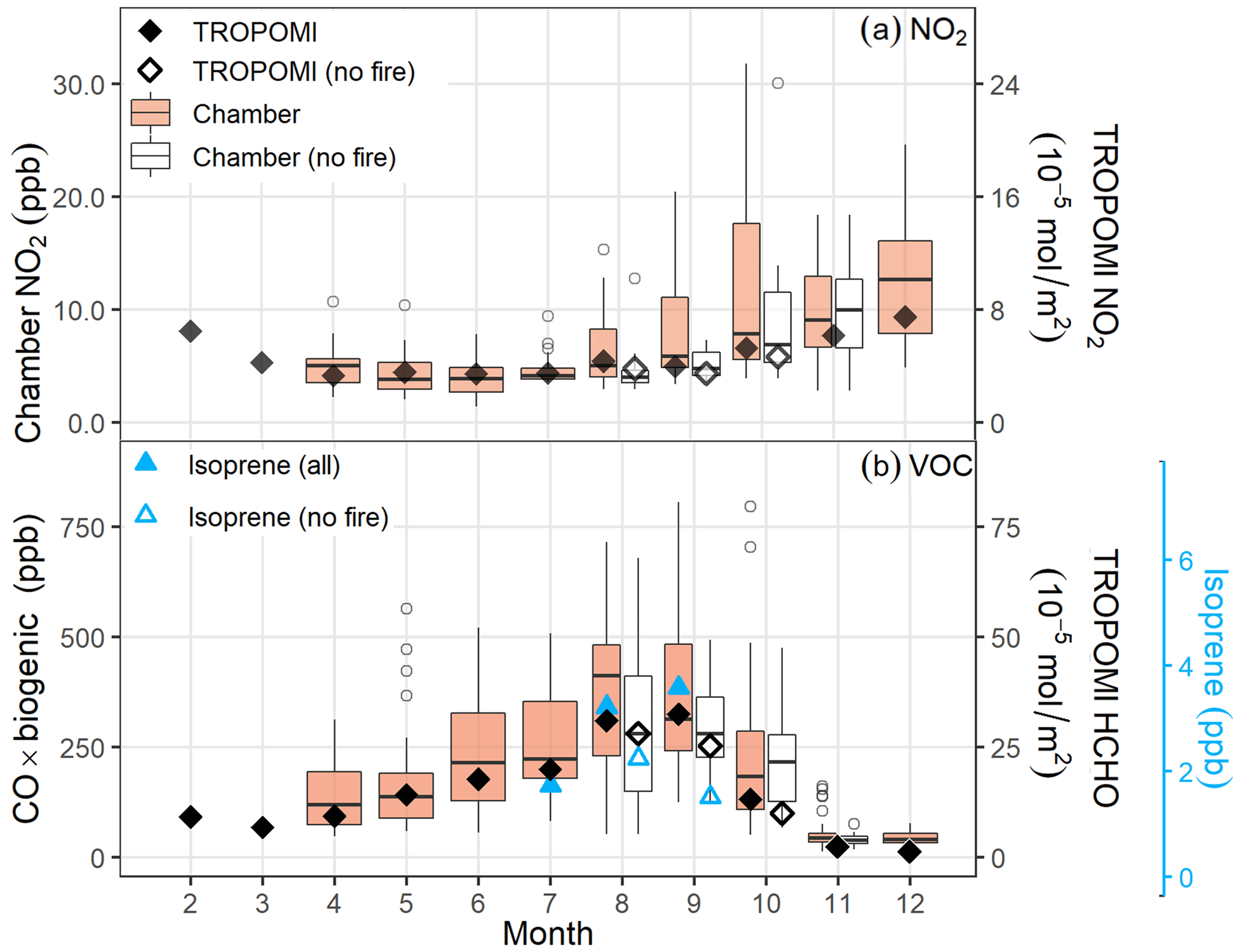
Figure 2 Monthly concentrations of NO₂ (a) and CO × biogenic/HCHO/isoprene (b) from February to December 2020. Ground-based chamber measurements use the left axis with results shown as box-and-whisker plots. TROPOMI measurements use the right axis and are shown as diamonds. Isoprene from the ground monitoring station is shown as blue triangles. The open box and points show the results after removing wildfire days.

3 Results

3.1 Chamber measurement and satellite results in Sacramento

3.1.1 Monthly variation of ambient gas concentrations

Figure 2 compares the ground-based measurements and the TROPOMI column measurements of NO_x and VOC surrogate concentrations at the Sacramento sampling site. Good agreement is observed between the time trends of the chamber and TROPOMI satellite remote sensing measurements. Both techniques identify strong seasonal patterns for the concentrations of the O₃ precursors.

Figure 2a shows the monthly-averaged TROPOMI satellite NO₂ measurements and the boxplot of daily chamber NO₂ measurements at Sacramento between February–December 2020. NO₂ concentrations remained relatively stable between April and July and then sharply increased in August–September possibly due to increased wildfires in the late summer months. Enrichment of NO₂ and other pollutants in wildfire plumes has been noted in previous research (Jaffe and Wigder, 2012). The open boxes in Fig. 2a represent days within the months of August–November that were not influenced by wildfire smoke (Anderson and Kuwayama, 2022), leading to reduced NO₂ concentrations. The upward trend in NO₂ concentrations in October–December 2020 is likely associated with decreased boundary layer heights and increased fuel consumption for heating during the colder fall–winter season. This seasonal association can also be viewed in the decreasing TROPOMI NO₂ levels measured during the warmer spring season (February–April, 2020). TROPOMI column measurements will not directly depend on boundary layer height, but increased boundary layer heights are usually associated with higher average boundary layer wind speeds, leading to downwind advection and dispersion of pollutants. The effects of reduced transportation emissions in March–April 2020 caused by COVID-19 shelter-in-place orders are notably minor in the ambient NO₂ measurements. Although light-duty vehicle traffic decreased by as much as 50 % during this time period, heavy-duty truck traffic was more constant (Liu et al., 2020; Parker et al., 2020). The ground-based measurement site is 0.8 and 1.8 km from two major freeways, but NO_x concentrations at this site do not appear to be strongly influenced by the COVID-19 reduction in light-duty traffic activity. Increasing NO_x emissions from residences and relatively quick recovery of the heavy-duty traffic compared to the light-duty traffic may also minimize COVID-19 effects on NO_x concentrations (Liu et al., 2021). The seasonal pattern of NO_x concentrations driven by wildfires, reduced boundary layer height, and increased residential fuel consumption appears to dominate at the urban Sacramento location.

Figure 2b shows the monthly-averaged TROPOMI satellite HCHO levels and the daily ground-based CO × biogenic concentration at the Sacramento sampling site. The agreement between the seasonal trend in the CO × biogenic and TROPOMI HCHO builds confidence in the use of CO × biogenic as a ground-based indicator of VOC concentrations at this location. Both indicators suggest that VOC concentrations increased from April–August 2020 and sharply declined in October 2020. Wildfires can emit large amounts of VOCs that can be transported to urban areas (Zhang et al., 2018). It is possible that wildfires contributed to the highest VOC concentrations observed between August and September 2020. Removing the days influenced by wildfires (open box) still leaves a strong seasonal trend with increasing VOC concentrations between April–August 2020, which is consistent with increasing VOC emissions from biogenic sources. Biogenic VOC (BVOC) emissions increase during warmer spring months and continue to increase as temperatures rise into summer (Guenther et al., 2006, 1991). The CO × biogenic factor inherently incorporates this effect, but the strong agreement between the TROPOMI HCHO levels and the CO × biogenic metric in Fig. 2b suggests that the seasonal pattern of the biogenic emissions is a real feature of the dataset and not an artifact of how the CO × biogenic metric was constructed. Similarly, the declining VOC concentration observed in October 2020 and beyond matched the expected decrease in biogenic emissions during the colder fall and winter seasons when vegetation becomes dormant. The seasonal pattern illustrated in Fig. 2b suggests that BVOC is an important precursor of HCHO in Sacramento.

PAMS measurements of ground-level isoprene concentrations in Sacramento are shown as blue diamonds in Fig. 2b. Isoprene is highly reactive in the atmosphere, and so PAMS-measured concentrations are lower than 4 ppb. The limited time period of available measurements makes it difficult to discern seasonal trends, but the slightly lower measured isoprene concentrations in July and slightly higher isoprene concentrations in August followed by decreasing (non-wildfire) isoprene concentrations in September generally match the VOC trends generated using both TROPOMI HCHO and CO × biogenic. Once again, the agreement between the three independent techniques builds confidence in the overall assessment of VOC seasonal trends.

Volatile chemical products (VCPs) are another important category of VOC emissions (McDonald et al., 2018). The expanded usage of spray disinfectant and sanitization products during the COVID-19 pandemic might have been a significant source of VOCs in the urban area, but the expected usage pattern of these products does not include a sharp decline in the fall period. The seasonal pattern of VOC concentrations increasing during spring–summer and decreasing during fall–winter is more consistent with a combination of biogenic sources and wildfires, as discussed above.

3.1.2 Seasonal trends in O₃ sensitivity

Figure 3a shows the monthly trends in measured ΔO${}_{\mathrm{3}}^{+{\text{NO}}_x}$ and TROPOMI $\mathrm{HCHO}/{\mathrm{NO}}_{\mathrm{2}}$ from February 2020 to December 2020 at the Sacramento site. The ΔO${}_{\mathrm{3}}^{+{\text{NO}}_x}$ value represents the change in O₃ concentrations in response to a +8 ppb NO_x perturbation. O₃ formation is NO_x-limited when the ΔO${}_{\mathrm{3}}^{+{\text{NO}}_x}$ value is positive and VOC-limited when the ΔO${}_{\mathrm{3}}^{+{\text{NO}}_x}$ value is negative. Changes in the absolute magnitudes of the ΔO${}_{\mathrm{3}}^{+{\text{NO}}_x}$ values reflect the degree of O₃ sensitivity to the NO_x perturbation. ΔO${}_{\mathrm{3}}^{+{\text{NO}}_x}$ and TROPOMI $\mathrm{HCHO}/{\mathrm{NO}}_{\mathrm{2}}$ both increase from April to August 2020 and then sharply decline in October 2020. By comparing the transition points of ΔO${}_{\mathrm{3}}^{+{\text{NO}}_x}=\mathrm{0}$ and TROPOMI $\mathrm{HCHO}/{\mathrm{NO}}_{\mathrm{2}}$ =4.6 (discussed in Sect. 3.2), it is evident that O₃ formation evolved from VOC-limited conditions in spring towards NO_x-limited conditions from June to August, followed by a return to VOC-limited conditions after October 2020. It is notable that the seasonal trend for ΔO${}_{\mathrm{3}}^{+{\text{NO}}_x}$ matches the trend of increased BVOC emissions during the summer and increased NO_x emissions during the winter. The travel restrictions associated with COVID-19 that occurred in March–May 2020 appeared to have little impact on the overall seasonal trends in ΔO${}_{\mathrm{3}}^{+{\text{NO}}_x}$ behavior.

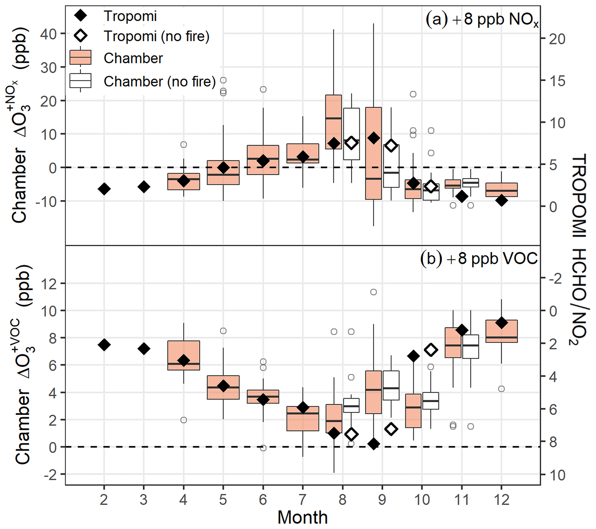
Figure 3 Monthly variation of TROPOMI $\mathrm{HCHO}/{\mathrm{NO}}_{\mathrm{2}}$ (diamond) and ΔO₃ (box) due to NO_x addition (ΔO${}_{\mathrm{3}}^{+{\text{NO}}_x}$, a) and VOC addition (ΔO${}_{\mathrm{3}}^{+\text{VOC}}$, b) from April to December including wildfire days (shaded box) and without wildfire days (open box).

The median ground-based ΔO${}_{\mathrm{3}}^{+{\text{NO}}_x}\mathit{<}\mathrm{0}$ indicates VOC-limited conditions in September 2020, but the TROPOMI satellite $\mathrm{HCHO}/{\mathrm{NO}}_{\mathrm{2}}$ >4.6 indicates NO_x-limited conditions for this same month. Removing the wildfire days from the analysis period (open box in Fig. 3a) did not reconcile the two measurements. The divergence of the ground-based measurements and satellite measurements in this month may reflect the presence of elevated plumes of wildfire smoke above the monitoring site that were detected by the satellite measurements (Jin et al., 2017). Cleaner air at the ground-based monitors, therefore, yielded ΔO${}_{\mathrm{3}}^{+{\text{NO}}_x}$ values in a different chemical regime than the satellite measurements that are based on the tropospheric vertical column densities. This comparison suggests that ground-based measurements may be required to supplement satellite-based measurements to fully characterize the surface O₃ formation regime under special circumstances that generate concentrated pollution layers above the ground-level.

Removing the days influenced by wildfires from the chamber measurement (open box) and TROPOMI satellite measurement (open diamond) in Fig. 3a reduces both ΔO${}_{\mathrm{3}}^{+{\text{NO}}_x}$ and TROPOMI $\mathrm{HCHO}/{\mathrm{NO}}_{\mathrm{2}}$. Figure S7 in the Supplement compares TROPOMI HCHO and NO₂ on wildfire days and non-wildfire days. Median TROPOMI HCHO measurements increased by 44 % and TROPOMI NO₂ measurements increased by 14 % on wildfire days. The comparison between wildfire vs. non-wildfire days implies that wildfires emit more VOC than NO_x, which is in agreement with previous studies (Jaffe and Wigder, 2012). It is also notable that the decrease in ΔO${}_{\mathrm{3}}^{+{\text{NO}}_x}$ is larger than the decrease in TROPOMI $\mathrm{HCHO}/{\mathrm{NO}}_{\mathrm{2}}$. This observation might once again reflect the fact that the wildfire identification algorithm (Anderson and Kuwayama, 2022) was based on ground-level measurements that do not flag all of the days with elevated plumes above the monitoring site that could differentially affect the satellite measurements.

Figure 3b shows the monthly variation of ground-based ΔO${}_{\mathrm{3}}^{+\text{VOC}}$ and TROPOMI satellite $\mathrm{HCHO}/{\mathrm{NO}}_{\mathrm{2}}$ from February–December 2020 at the Sacramento sampling site. ΔO${}_{\mathrm{3}}^{+\text{VOC}}$ (Fig. 3b) has an inverse time trend compared to ΔO${}_{\mathrm{3}}^{+{\text{NO}}_x}$ and TROPOMI $\mathrm{HCHO}/{\mathrm{NO}}_{\mathrm{2}}$ (Fig. 2a). The ΔO${}_{\mathrm{3}}^{+\text{VOC}}$ trend is well correlated to the TROPOMI $\mathrm{HCHO}/{\mathrm{NO}}_{\mathrm{2}}$ trend plotted on a reversed axis between April–August 2020, but the two trends diverge in September–October 2020 when wildfires were prevalent. Removing the wildfire days from August to October (open box) increased the ground-based ΔO${}_{\mathrm{3}}^{+\text{VOC}}$, once again suggesting that wildfires contributed more VOCs than NO_x to the atmosphere (Altshuler et al., 2020). The divergence between the ground-based ΔO${}_{\mathrm{3}}^{+\text{VOC}}$ measurements and TROPOMI satellite $\mathrm{HCHO}/{\mathrm{NO}}_{\mathrm{2}}$ measurements during the wildfire season once again reflects the presence of elevated plumes that were measured by the satellite but not by the ground-based monitors (Schroeder et al., 2017a).

3.1.3 Weekend effect

Figure 4 separately plots concentrations of O₃ precursors and O₃ sensitivity on weekdays (shaded bars) and weekends (open bars) during the current study period. Direct wildfire days have been removed from the analysis (Anderson and Kuwayama, 2022) to focus on the day-of-week patterns. Hypothesis tests were carried out to determine if weekday and weekend responses were similar in each month. The results indicate that weekend reductions in NO₂ concentrations were significant at a 90 % confidence level (or higher) before July. The similarity between weekday and weekend NO₂ concentrations after July may be associated with increased NO_x emissions from wildfires in the late summer and space heating in the fall–winter since neither of these sources follows a weekday/weekend pattern. Although days directly affected by the wildfire smoke were removed from the analysis, residual emissions from smoldering fires and multi-day recirculation of air mass that have been affected by wildfire smoke may have contributed to elevated regional NO_x concentrations through the formation of reactive nitrogen reservoir species such as peroxyacetyl nitrate (PAN) that can be transported over long distances (Lindaas et al., 2017). The CO × biogenic VOC surrogate did not display statistically significant differences between weekdays vs. weekends except in June and July. Extremely hot days (>35 ^∘C) occurred on weekdays in June and weekends in July, driving the CO × biogenic factor higher.

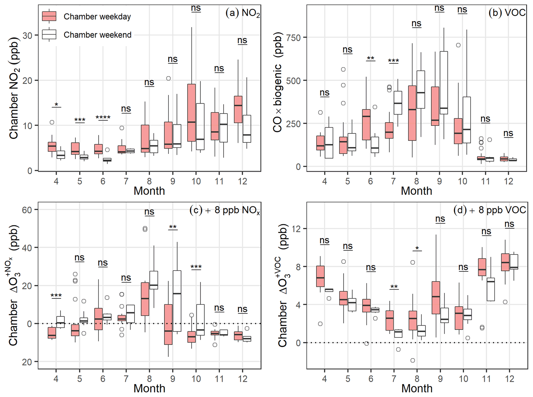
Figure 4 Weekday (solid box) and weekend (open box) monthly-average concentrations of NO₂ and CO × biogenic (a, b) and ΔO${}_{\mathrm{3}}^{+}$NO_x and ΔO${}_{\mathrm{3}}^{+\mathrm{VOC}}$ (c, d) from April to December 2020 after removing wildfire days. The asterisks above each box-and-whisker plot represent the significance of the weekday vs. weekend difference. ($\ast :p$ value <0.1; $\ast \ast :p$ value <0.05; $\ast \ast \ast :p$ value <0.01; $\ast \ast \ast \ast :p$ value <0.001; ns (not significant): p value >=0.1).

Reduced NO_x emissions on weekends are reflected in the O₃ sensitivity to precursors shown in Fig. 4c and d. The median ΔO${}_{\mathrm{3}}^{+{\mathrm{NO}}_x}$ sensitivity is higher on weekends for most months, indicating that the atmosphere was more NO_x-limited. Large variability in the data makes the weekend vs. weekday ΔO${}_{\mathrm{3}}^{+{\mathrm{NO}}_x}$ response statistically significant at the 90 % (or higher) level only in April, September, and October. The large weekend reductions in median NO₂ concentrations detected in May and June did not lead to significantly higher weekend ΔO${}_{\mathrm{3}}^{+{\text{NO}}_x}$, possibly because of higher weekday median VOC concentrations in these months. Median O₃ sensitivity was NO_x-limited (ΔO${}_{\mathrm{3}}^{+{\text{NO}}_x}\mathit{>}\mathrm{0}$) on both weekdays and weekends from June to August when BVOC emissions are expected to be highest. In spring and early fall (April, May, and September), the median weekday O₃ sensitivity is VOC-limited but the median weekend O₃ sensitivity is NO_x-limited. In late fall and winter (October–November), the median O₃ sensitivity is VOC-limited on both weekends and weekdays. Weekend NO_x reductions have an inverse effect on ΔO${}_{\mathrm{3}}^{+\text{VOC}}$ shown in Fig. 4d compared to ΔO${}_{\mathrm{3}}^{+{\text{NO}}_x}$. The median ΔO${}_{\mathrm{3}}^{+\text{VOC}}$ is lower on weekends than weekdays because the O₃ formation is more NO_x-limited on weekends.

3.1.4 O₃ isopleth measurements

Figure 5 summarizes the NO_x, CO × biogenic, O₃, ΔO${}_{\mathrm{3}}^{+{\text{NO}}_x}$, and ΔO${}_{\mathrm{3}}^{+\text{VOC}}$ measurements in Sacramento from April to December in 2020 in the format of an O₃ isopleth diagram. Each data point in Fig. 5 corresponds to measurements on a single day. The color of each symbol represents the O₃ concentration in the base case chamber after 3 h of UV irradiation. The NO_x and CO × biogenic factors are calculated as the daily value divided by averaged value. The arrow attached to each data symbol points in the direction of maximum ΔO₃ in response to NO_x and VOC addition. The magnitude of the arrow corresponds to the strength of the ΔO₃ response. All arrows generally point right, meaning that VOC addition increased O₃ concentrations. Arrows pointing to the bottom right indicate that NO_x addition decreased the O₃ concentration, while arrows pointing to the upper right indicate that NO_x addition increased the O₃ concentrations. The most effective emissions control program acts in the direction opposite to each arrow.

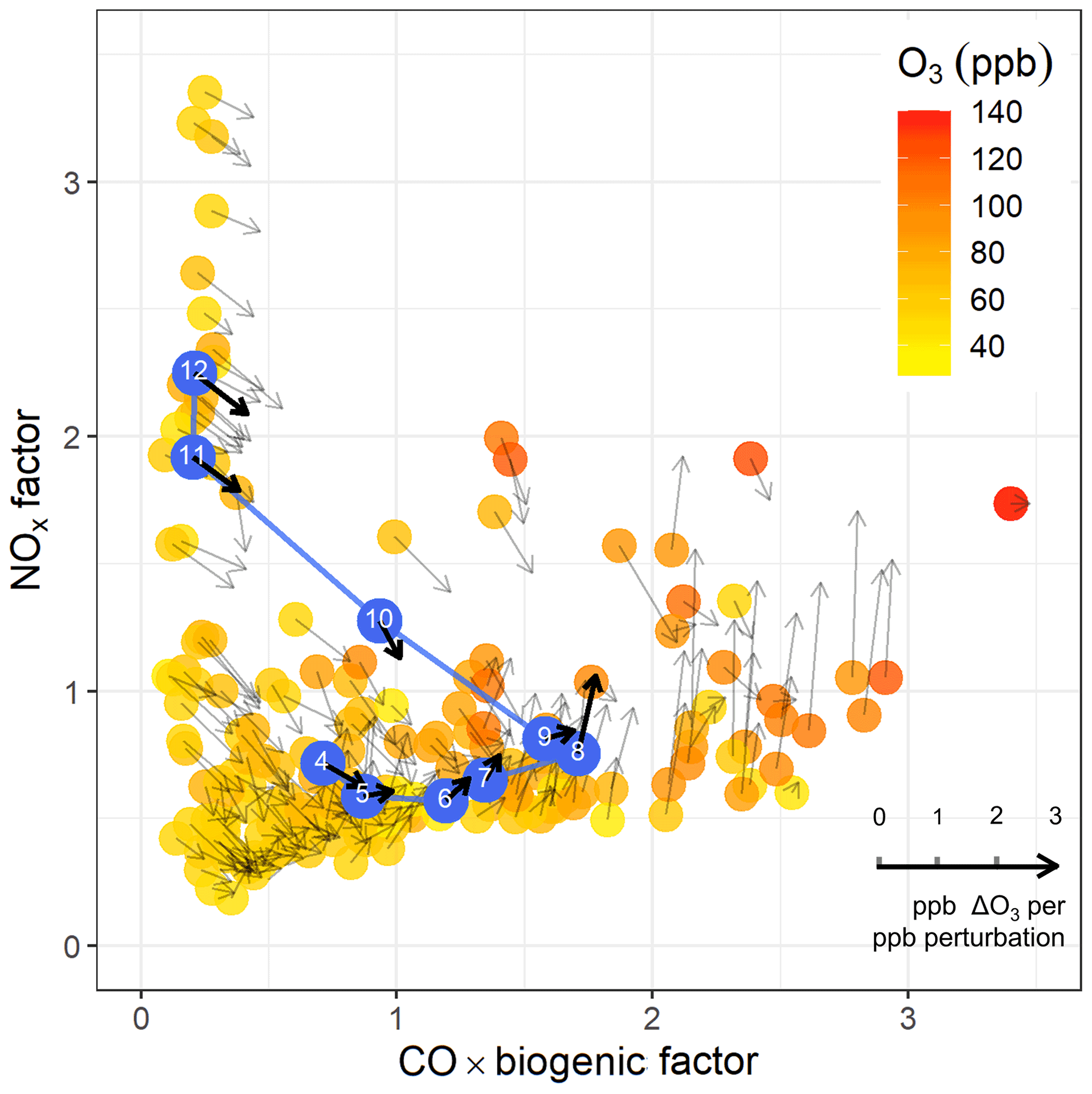
Figure 5 Measured O₃ isopleth diagram. The NO_x and CO × biogenic factor is calculated by the daily value divided by averaged value. The O₃ concentration is the daily O₃ concentration in the base case chamber after 3 h UV exposure. Arrows represent the O₃ sensitivity. The blue dots are the monthly-averaged values, and the blue line shows the seasonal cycle in the O₃ isopleth diagram. Days influenced by wildfires are removed from the plot.

The mixture of daily data points (yellow to red points) shows the O₃ isopleth pattern where higher O₃ concentration (darker color) exists at higher NO_x and VOC concentrations. The combination of the colors and the arrows illustrated in the isopleth diagram helps to define the measured ridgeline in the O₃ isopleth diagram that denotes the transition between VOC-limited chemistry and NO_x-limited chemistry at Sacramento. Arrows in the upper left of the diagram point downwards (VOC-limited) towards the ridgeline, while arrows in the lower right of the diagram point upwards (NO_x-limited) towards the ridgeline. The atmospheric system experiences a range of conditions throughout the 9-month study period that moved the measurements around the O₃ isopleth diagram. The average seasonal cycle is illustrated in Fig. 5 using monthly-average points shown as blue circles with white month numbers. The monthly-average O₃ chemical regime traces an oval path through the isopleth diagram as NO_x concentrations decrease and CO × biogenic (proxy of VOC) concentrations increase moving from spring to summer months. NO_x concentrations increase rapidly in fall while CO × biogenic concentrations simultaneously decrease at the Sacramento sampling location, transitioning the O₃ chemistry to VOC-limited conditions. The pattern is expected to reverse for the months of January–March (not shown) to produce a repeatable annual cycle. The direct measurement of the seasonal pattern of the O₃ chemical regime clearly illustrates the effects of NO_x and VOC emissions controls at different times of the year.

3.1.5 Extreme value analysis for O₃ sensitivity

The days with the highest measured O₃ concentrations are of particular interest in the current study since emissions control programs are traditionally tailored to reduce the O₃ design value, which is determined by MDA8 O₃ concentration. Figure 6 illustrates box-and-whisker plots of measured ΔO${}_{\mathrm{3}}^{+{\text{NO}}_x}$ and ΔO${}_{\mathrm{3}}^{+\text{VOC}}$ at Sacramento binned according to the MDA8 O₃ concentration measured at the monitoring station near the chamber measurement site. The right two bins, corresponding to the O₃-nonattainment days (MDA8 O₃>70 ppb), have O₃ sensitivity in the NO_x-limited regime where NO_x addition increases O₃ concentrations and VOC addition has minor effects on O₃ concentrations. These measurements suggest that a NO_x emissions control strategy would be most effective at reducing these peak O₃ concentrations. In contrast, a large portion of the days with MDA8 O₃ concentrations below 55 ppb were in the VOC-limited regime, suggesting that an emissions control strategy focusing on NO_x reduction would increase O₃ concentrations. VOC controls on these intermediate days would be difficult, however, if biogenic VOCs account for the majority of the O₃ formation. This challenging situation suggests that emissions control programs that focus on NO_x reductions will immediately lower peak O₃ concentrations but slightly increase intermediate O₃ concentrations until NO_x levels fall far enough to re-enter the NO_x-limited regime.

Figure 6 Boxplot of O₃ sensitivity to NO_x and VOC as a function of MDA8 O₃ concentration. Points indicate the data point in each range of MDA8 O₃ concentration.

Additional statistical analysis was carried out to characterize the extreme values in the O₃ sensitivity plots (Coles, 2001; Gilleland and Katz, 2016). Extreme value analysis characterizes high concentrations using return levels corresponding to a specified time period (T). In the context of the current analysis, the return level is the ΔO₃ perturbation response that is expected to be exceeded once during the specified time period. The probability of exceeding the return level is therefore $\mathrm{1}/T$. Figure 7 shows the 90 d return level for ΔO${}_{\mathrm{3}}^{+{\mathrm{NO}}_x}$ and ΔO${}_{\mathrm{3}}^{+\text{VOC}}$ sensitivity based on statistical analysis of the measured perturbation response in each month. The 90 d time period was chosen to correspond to the time period inherent in the O₃ design value values that are based on the annual fourth-highest O₃ concentration averaged in 3 years (12 exceedances $/$ 1095 d equals approximately 1 exceedance $/$ 90 d). The 90 d return value of O₃ sensitivity can therefore be viewed as the design value for O₃ sensitivity. Figure 7 shows that the 90 d return levels for O₃ sensitivity and the median O₃ sensitivity follow similar seasonal trends, but the extreme values are shifted higher such that they are NO_x-limited from April to December, except November, which is slightly VOC-limited. The positive 90 d return levels of ΔO${}_{\mathrm{3}}^{+{\text{NO}}_x}$ once again suggest the NO_x control is an efficient strategy to reduce peak O₃ concentrations in Sacramento.

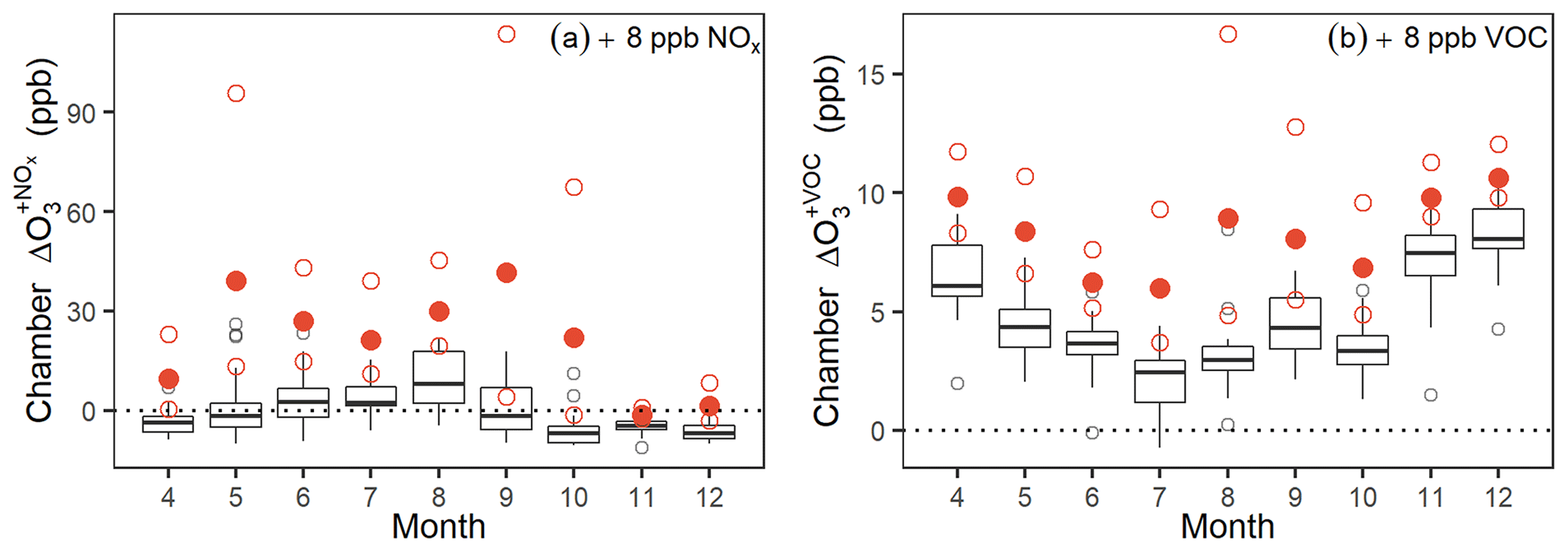
Figure 7 Three-year return level (red dot) and 95 % confidence interval (red open dot) from extreme value analysis of O₃ sensitivity to NO_x and VOC.

3.2 Chamber and TROPOMI data correlation

The consistency between the NO_x and VOC measurements made using ground-based chambers and satellite observations enables a joint analysis to directly calculate the TROPOMI $\mathrm{HCHO}/{\mathrm{NO}}_{\mathrm{2}}$ ratio at the transition between NO_x and VOC-limited O₃ formation regimes. Three circular buffers (2.5, 5, and 7.5 km radii) centered on the monitoring location were used to generate the TROPOMI $\mathrm{HCHO}/{\mathrm{NO}}_{\mathrm{2}}$ ratio that was then compared to the measured ΔO${}_{\mathrm{3}}^{+{\text{NO}}_x}$ ratio at the monitoring site. The $\mathrm{HCHO}/{\mathrm{NO}}_{\mathrm{2}}$ ratio generated using the 5 km radius buffer shows the best correlation with ground-based chamber results shown in Fig. 8a (results from other buffers are shown in Fig. S8 in the Supplement). Linear regression analysis between 1-week-averaged ΔO${}_{\mathrm{3}}^{+{\text{NO}}_x}$ and $\mathrm{HCHO}/{\mathrm{NO}}_{\mathrm{2}}$ with and without wildfires shows that removing the wildfires always improves the correlation coefficient (R), likely because the elevated wildfire plumes have different effects on surface vs. integrated column measurements. The regression carried out using a 5 km buffer radius with wildfires removed yielded a correlation coefficient R=0.62 (p<0.001). The transition point between NO_x-limited and VOC-limited conditions (corresponding to ΔO${}_{\mathrm{3}}^{+{\text{NO}}_x}=\mathrm{0}$) occurs when $\mathrm{HCHO}/{\mathrm{NO}}_{\mathrm{2}}$ =4.6 (95 % confidence interval: 4.39–5.90). When the TROPOMI satellite $\mathrm{HCHO}/{\mathrm{NO}}_{\mathrm{2}}$ ratio fell below 4.6, then the ground-based measurement of ΔO${}_{\mathrm{3}}^{+{\text{NO}}_x}$ was usually negative, and when the satellite $\mathrm{HCHO}/{\mathrm{NO}}_{\mathrm{2}}$ ratio rose above 4.6, then the ground-based measurement of ΔO${}_{\mathrm{3}}^{+{\text{NO}}_x}$ was usually positive. Ordinary lease squares (OLS) regression was used to estimate the transition point $\mathrm{HCHO}/{\mathrm{NO}}_{\mathrm{2}}$ =4.6 between chemical regimes. This approach does not account for uncertainty in chamber ΔO${}_{\mathrm{3}}^{+{\text{NO}}_x}$. Repeating the analysis using reduced major axis (RMA) regression that accounts for errors in both x and y yields an estimated transition point $\mathrm{HCHO}/{\mathrm{NO}}_{\mathrm{2}}$ =4.4 between chemical regimes (Fig. S9 in the Supplement).

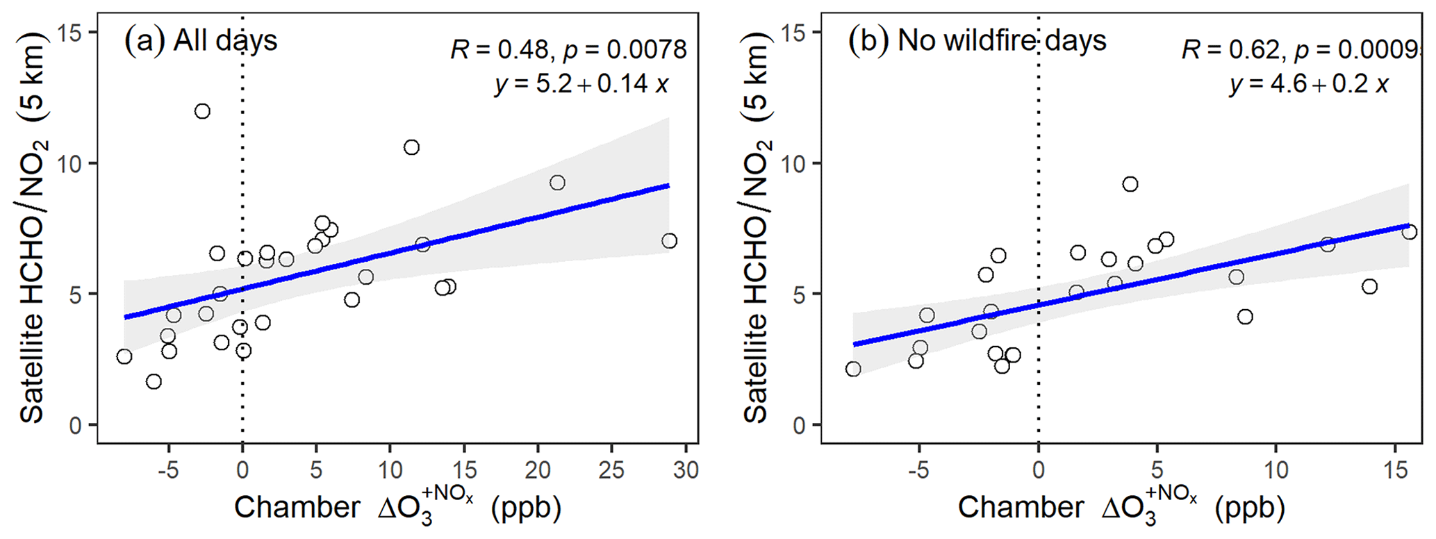
Figure 8 Ordinary least squares (OLS) regression between weekly-averaged TROPOMI $\mathrm{HCHO}/{\mathrm{NO}}_{\mathrm{2}}$ at 5 km circular buffers and the weekly-averaged ΔO${}_{\mathrm{3}}^{+{\text{NO}}_x}$ from ground-based measurement. The shaded area shows the 95 % confidence interval of the mean response of the predicted value.

The $\mathrm{HCHO}/{\mathrm{NO}}_{\mathrm{2}}$ transition point directly measured in the current study is consistent with previous estimates constructed from the combination of satellite measurements and routine ground-based O₃ monitoring data (Jin et al., 2020). Other previous efforts to estimate $\mathrm{HCHO}/{\mathrm{NO}}_{\mathrm{2}}$ value at the transition point between NO_x-limited and VOC-limited regimes typically couple satellite $\mathrm{HCHO}/{\mathrm{NO}}_{\mathrm{2}}$ measurements with O₃ sensitivity or O₃ sensitivity indicators (i.e., ${\mathrm{LNO}}_x/{\mathrm{LRO}}_x$) predicted using reactive chemical transport models. These hybrid studies predict $\mathrm{HCHO}/{\mathrm{NO}}_{\mathrm{2}}$ transition points lower than the value of 4.6 derived in the current study. Martin (2004) used $\mathrm{HCHO}/{\mathrm{NO}}_{\mathrm{2}}$ from GOME to calculate the regime transition value $\mathrm{HCHO}/{\mathrm{NO}}_{\mathrm{2}}$ =1.0 for polluted areas across the globe. Duncan et al. (2010) used OMI to estimate the regime transition value $\mathrm{HCHO}/{\mathrm{NO}}_{\mathrm{2}}$ =1–2 across the continental United States. Schroeder (2017b) found the transition range could between $\mathrm{HCHO}/{\mathrm{NO}}_{\mathrm{2}}$ =1.3–5.0 during DISCOVER-AQ in Houston. These estimated $\mathrm{HCHO}/{\mathrm{NO}}_{\mathrm{2}}$ transition values vary due to the different satellite resolution, retrieval algorithms, and inherent air pollution patterns over the different study areas. The finer-resolution satellite data used in the current study combined with direct ground-based measurements of O₃ sensitivity should provide accurate information for the $\mathrm{HCHO}/{\mathrm{NO}}_{\mathrm{2}}$ transition point between chemical regimes over California.

3.3 TROPOMI O₃ sensitivity in California

Figure 9 displays the monthly-average spatial distribution of TROPOMI $\mathrm{HCHO}/{\mathrm{NO}}_{\mathrm{2}}$ ratios across California for the time period April–October 2020. Overall, TROPOMI $\mathrm{HCHO}/{\mathrm{NO}}_{\mathrm{2}}$ was the lowest (mean (standard deviation) =3.5 (1.2)) in April and the highest (mean (standard deviation) =9.7 (3.2)) in July. The seasonal pattern of increasing NO_x limitation during the summer months at Sacramento (Fig. 3a, b) is mirrored across most of California (Fig. 9), especially in the mountainous areas with dense vegetation. The majority of California is in the VOC-limited regime in April and May due to the low BVOC emissions. Only very remote regions with low NO_x concentrations are still in the NO_x-limited regime during these spring months. Most areas outside of major urban centers transition toward NO_x-limited conditions between June and September as ambient temperature and BVOC emissions increase. These areas then transition back to the VOC-limited regime in the fall months beginning in October as temperatures decrease and vegetation becomes dormant.

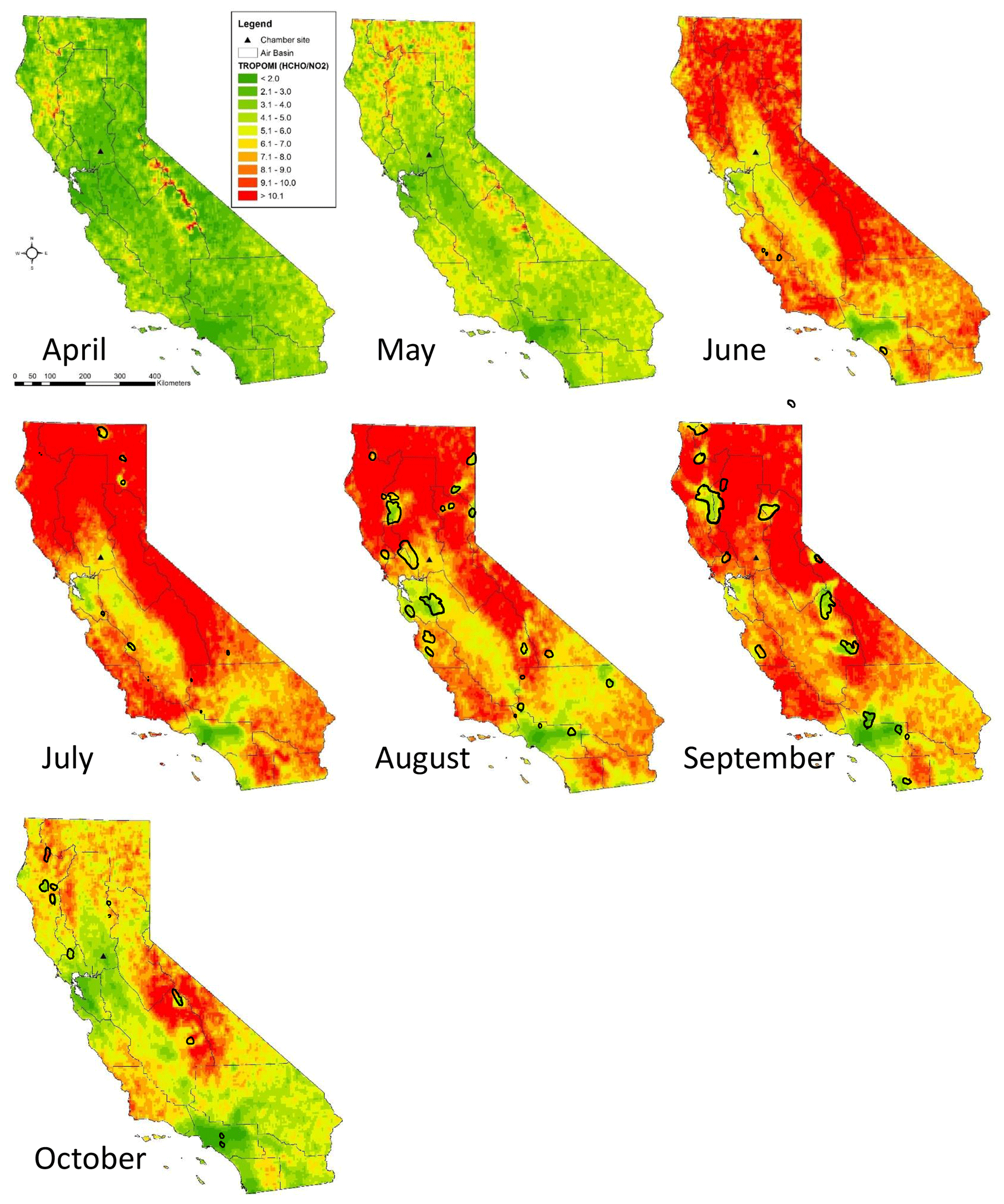
Figure 9 Spatial distribution of TROPOMI satellite ($\mathrm{HCHO}/{\mathrm{NO}}_{\mathrm{2}}$) ratios in California for April–October 2020. TROPOMI NO₂ and HCHO data are re-gridded to 5 km resolution when calculating monthly-average ratios. The black bold line circles the burned area in each month detected by MODIS from Fire Information for Resource Management System (FIRMS). The NO_x-limited conditions correspond to $\mathrm{HCHO}/{\mathrm{NO}}_{\mathrm{2}}$ ratios above 4.6.

Large urban centers including Los Angeles, San Diego, and the San Francisco Bay Area exhibit low $\mathrm{HCHO}/{\mathrm{NO}}_{\mathrm{2}}$ ratios (VOC-limited conditions) throughout the study period. These urban areas contain less vegetation and larger numbers of NO_x sources than outlying suburban and rural areas. Therefore, reducing NO_x emissions in these urban centers may increase monthly-average O₃ concentrations throughout the year. The $\mathrm{HCHO}/{\mathrm{NO}}_{\mathrm{2}}$ ratio in California's Central Valley is lower than the $\mathrm{HCHO}/{\mathrm{NO}}_{\mathrm{2}}$ ratio in the surrounding mountainous area during all months of the study period. This spatial pattern reflects the high BVOC emissions from coniferous forests in the mountainous regions compared to the cropland in the Central Valley (Misztal et al., 2014).

Past studies have found that wildfire smoke plumes mixing with high urban NO_x emissions can lead to enhanced urban O₃ concentrations (Jaffe and Wigder, 2012). The effects of wildfires during August–September 2020 can be observed in Fig. 9 as zones of reduced $\mathrm{HCHO}/{\mathrm{NO}}_{\mathrm{2}}$ immediately around the active burn areas followed by a larger halo zone of increased $\mathrm{HCHO}/{\mathrm{NO}}_{\mathrm{2}}$ as the VOCs emitted from wildfires have time to react to form HCHO. This halo pattern is most obvious in October 2020, when the seasonal cycle of biogenic emissions declined sufficiently to shift the O₃ sensitivity back to the VOC-limited regime for the majority of the state except for the region surrounding a wildfire in the Sierra Nevada mountain range east of Fresno (near Yosemite National Park). VOCs emitted from the wildfire in October 2020 reacted to produce HCHO in the halo region, keeping the $\mathrm{HCHO}/{\mathrm{NO}}_{\mathrm{2}}$ ratio in the NO_x-limited regime. The extensive wildfires that occurred in 2020 appear to have extended the natural peak of the $\mathrm{HCHO}/{\mathrm{NO}}_{\mathrm{2}}$ ratio from July into August, September, and even October 2020. It is unknown whether this satellite observation accurately represents conditions at ground level. The results at the Sacramento monitoring site in September 2020 (Fig. 3a and b) suggest that elevated smoke plumes can dominate the satellite observations, but they may not accurately represent conditions at ground level.

The seasonal variation of O₃ sensitivity can be observed over the entire state of California using the TROPOMI $\mathrm{HCHO}/{\mathrm{NO}}_{\mathrm{2}}$ (Table S1). Figure 10a shows how the O₃ sensitivity seasonal pattern differs among different air basins. The air basins with the highest populations have suppressed seasonal variation of O₃ sensitivity because of the higher anthropogenic NO_x emissions. The SoCAB had the lowest $\mathrm{HCHO}/{\mathrm{NO}}_{\mathrm{2}}$ ratio among all the air basins in California during the study period. This is noteworthy since the SoCAB has the highest population and the highest O₃ concentrations. The San Francisco Bay Area and San Diego County, two other heavily populated areas in California, also have relatively low $\mathrm{HCHO}/{\mathrm{NO}}_{\mathrm{2}}$ ratios compared to other air basins. Using $\mathrm{HCHO}/{\mathrm{NO}}_{\mathrm{2}}$ =4.6 as the transition point, even these highly urbanized air basins appear to transition from VOC-limited to NO_x-limited O₃ formation chemistry in summer 2020. It is noteworthy, however, that the urban cores of these regions remain VOC-limited across all months due to very high NO_x emissions (see persistently green regions in Fig. 9). Figure 10b illustrates the TROPOMI $\mathrm{HCHO}/{\mathrm{NO}}_{\mathrm{2}}$ monthly variation for different cities in SoCAB between February and October 2020. The cities inside/around the LA urban core have $\mathrm{HCHO}/{\mathrm{NO}}_{\mathrm{2}}$ <4.6 throughout the entire year with a weak seasonal variation. This might be caused by reduced BVOC emissions in the urban center. The remote areas (darker colors in Fig. 10b) have greater seasonal variation and higher peak $\mathrm{HCHO}/{\mathrm{NO}}_{\mathrm{2}}$. The sharp increase in $\mathrm{HCHO}/{\mathrm{NO}}_{\mathrm{2}}$ in summer leads to a shift in O₃ sensitivity from the NO_x-saturated regime to the NO_x-limited regime in the cities further away from the urban core. Due to the different seasonal variation of $\mathrm{HCHO}/{\mathrm{NO}}_{\mathrm{2}}$ at different sites, the NO_x-saturated region around the urban core will shrink in the summer and expand in the winter. Figure S10 in the Supplement shows this seasonal pattern of O₃ sensitivity regime distribution in Los Angeles as an example. Thus, the optimal emissions control strategy for the entire air basin may differ from the optimal emissions control strategy for urban cores areas.

Figure 10 Monthly variation of TROPOMI $\mathrm{HCHO}/{\mathrm{NO}}_{\mathrm{2}}$ in different air basins (a) and in different cities in Southern California (b). The darker colors in the right panel indicate increasing distance from the urban center of Los Angeles.

4 Discussion

4.1 Sensitivity analysis

The chamber measurements made in the current study capture the sensitivity of the O₃ chemical production term in response to the concentration of NO_x and VOC. The experiment does not directly account for atmospheric processes such as mixing and deposition, but the chemical production term represents the dominant processes that determine how local emissions affect local O₃ concentrations. The good agreement between ground-based chamber measurements and satellite O₃ sensitivity measurements in the current study builds confidence in the reported seasonal trend of O₃ sensitivity. Limitations and uncertainties associated with the temperature, UV intensity, and ${\mathrm{NO}}_x/\mathrm{VOC}$ perturbations used in the ground-based chamber measurements are discussed in this section to build further confidence in the results. The potential of these issues to influence the results is analyzed through a combination of measurements and model calculations. The configuration of the chamber model is described in Sect. 2.4. Figure 11 shows that the chamber model can accurately predict the measured seasonal trends in O₃ sensitivity, providing a solid foundation for sensitivity tests.

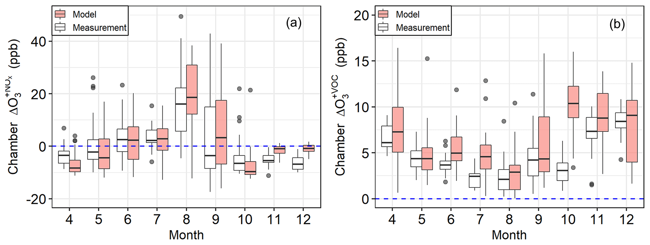
Figure 11 Monthly variation of the ΔO${}_{\mathrm{3}}^{+{\text{NO}}_x}$ (a) and ΔO${}_{\mathrm{3}}^{+\text{VOC}}$ (b) predicted by the chamber model (solid box) and directly measured in the chamber (open box) from April to December 2020 at the Sacramento measurement site.

4.1.1 Temperature

The temperature in the reaction chambers was higher than the ambient temperature due to the heating effects of the UV lights. Figure S11 in the Supplement shows that the difference between the chamber gas temperature and the ambient temperature increased by 5–10 ^∘C over the course of each experiment, with the exact temperature profile depending on the measurement month. Despite this temperature increase, all three chambers experience the same temperature profile, and so the comparison of O₃ formation between the chambers is not strongly biased by this issue. Figure 12a shows the calculated ΔO${}_{\mathrm{3}}^{+{\text{NO}}_x}$ during each month of the experiment under the chamber and ambient temperature profiles. The difference between the chamber and ambient temperature has little effect on the O₃ sensitivity in each month. Temperature effects do not significantly modify the seasonal variation of the measured O₃ sensitivity in the current study. Similar behavior was shown in ΔO${}_{\mathrm{3}}^{+\text{VOC}}$ in Fig. S12a.

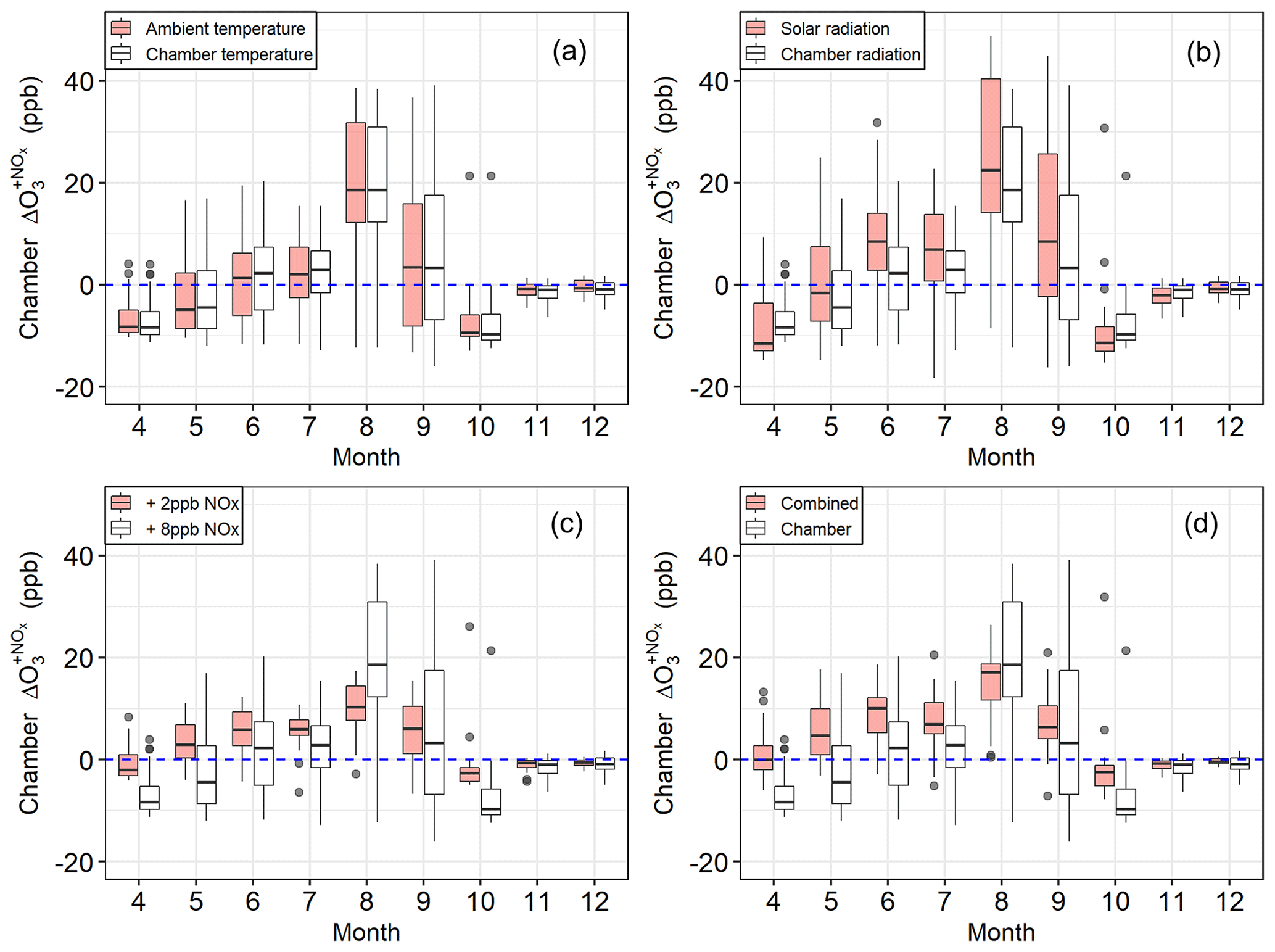
Figure 12 Effect of temperature, radiation, and perturbation amount on the monthly variation of the predicted chamber ΔO${}_{\mathrm{3}}^{+{\text{NO}}_x}$ from April to December 2020 at the Sacramento measurement site. Open boxes show the predicted response under chamber measurement conditions (chamber temperature, radiation, and 8 ppb NO₂ perturbation). Solid boxes show the predicted response when conditions are updated: (a) using the ambient temperature profile; (b) using clear-sky solar radiation; (c) using a 2 ppb NO_x perturbation; and (d) using the combination of ambient temperature, solar radiation, and 2 ppb NO₂ perturbation.

4.1.2 UV intensity

The UV intensity in the chambers was intentionally maintained at a constant level through all seasons so that the changes in O₃ sensitivity could be directly attributed to the changes in the ambient concentrations. A representative average UV intensity was selected for this purpose. As was the case with temperature, all chambers experience the same UV conditions, and so this factor is not expected to overly bias the comparison between chambers that acts as the core of the current study. The actual seasonal cycle of UV radiation would generate higher photolysis rates in the summer and lower photolysis rates in the winter that would further amplify the seasonal signal already detected by the measurements with constant UV intensity. SAPRC11 chamber model simulations were used to quantify the effect of seasonal variations in UV intensity. Simulations were carried out using the measured constant UV radiation in the chambers and using the clear-sky UV intensity calculated with the routines in the UCD/CIT CTM based on the latitude–longitude of the measurement site and the day of year. The calculations summarized in Fig. 12b show that the difference associated with the use of constant UV radiation does not change the seasonal pattern of O₃ sensitivity to NO_x perturbations. The seasonal changes to UV intensity slightly amplify the magnitude of the seasonal trend in O₃ sensitivity (increase the absolute value of ΔO${}_{\mathrm{3}}^{+{\text{NO}}_x}$), but the overall seasonal pattern is unchanged. Similar behavior was shown in ΔO${}_{\mathrm{3}}^{+\text{VOC}}$ in Fig. S12b in the Supplement.

4.1.3 Perturbation size

The constant 8 ppb NO₂ perturbations used in the current study are greater than or equal to ambient NO_x concentrations during the summer season at Sacramento. O₃ formation chemistry is non-linear, meaning that the size of the perturbation may complicate the interpretation of the sensitivity results. O₃ sensitivity measurements were conducted using NO_x perturbations ranging from 1–10 ppb at the UC Davis campus from December 2021 to January 2022 to investigate the non-linear behavior of the O₃ formation chemistry. The results summarized in Fig. S13 in the Supplement show the O₃ response expressed as ΔO₃ (final O₃ concentration in the base case chamber minus final O₃ concentration in the NO_x perturbed chamber). The ΔO₃ is negative in all NO_x perturbed tests due to the low VOC emission in winter in Davis, CA (similar to Sacramento). Increasing the magnitude of the NO_x perturbation increased the absolute magnitude of the ΔO₃ value but did not shift the chemistry into a different regime.

The size of the NO_x and VOC perturbation used in the chamber experiments is most important when ambient conditions are close to the ridgeline on the O₃ isopleth diagram (spring and fall in the current experiment). An 8 ppb NO₂ perturbation may jump over the ridgeline in this case, suggesting that the chemistry is NO_x-rich rather than NO_x-limited. SAPRC11 chamber model simulations were used to quantify the effect of the 8 ppb NO₂ perturbation vs. a smaller 2 ppb NO₂ perturbation. As shown in Fig. 12c, the 8 ppb NO₂ perturbations used in the current study do not affect the shape of the seasonal trend in O₃ sensitivity measurement, but the 8 ppb NO₂ perturbation (open box in Fig. 12c) does affect the transition months when the atmospheric system changes to NO_x-limited behavior. This issue may influence the estimated value of $\mathrm{HCHO}/{\mathrm{NO}}_{\mathrm{2}}$ that characterizes the transition to NO_x-limited behavior in Sect. 3.2, but it should be noted that the value of 4.6 derived in the current study is in good agreement with the value of 4.5 reported by Jin et al. (2020). The non-linearities associated with VOC chemistry are less severe, and so the size of the VOC perturbation does not complicate the interpretation of results (see ΔO${}_{\mathrm{3}}^{+\text{VOC}}$ in Fig. S12c).

4.1.4 Combined effects of temperature, UV intensity, and perturbation size

The O₃ sensitivity calculated with the combined effects of temperature, UV intensity, and lower perturbation size was compared to the base case calculated O₃ sensitivity in Figs. 12d and S12d (in the Supplement). The NO₂ perturbation size has the largest effect on the chamber O₃ sensitivity results, with relatively minor changes introduced by temperature and UV intensity. None of these issues changes the basic pattern of increasing NO_x limitations during summer months transitioning to VOC limitations during winter months. It should be noted that operation of the mobile smog chamber system in cities with higher ambient NO_x concentrations is expected to give O₃ sensitivity results that are even less dependent on the NO₂ perturbation size.

4.2 O₃ control strategies in California

California's current O₃ control strategies mainly focus on NO_x emissions from motor vehicles (Barcikowski et al., 2017) and especially heavy-duty trucks (Burke, 2020). Additional control strategies would require cleaner engines and zero/near-zero emission technologies (Brown, 2018; South Coast AQMD, 2021). VOC sources that dominate O₃ formation are still not clear due to the large numbers of activities that release VOCs and the complex reactions that VOCs undergo in the atmosphere. Controls on VOC emissions have been more effective than controls on NO_x emissions over the past decades, mainly because of reduced emissions from large stationary sources (Barcikowski et al., 2017). The estimated VOC emissions decreased by a factor of 3 while NO_x emission decreased by a factor of 1.5 between 1980 and 2010 according to the California inventory (Cox et al., 2013; Rasmussen et al., 2013). Long-term ambient measurements in the SoCAB confirm that ambient VOC concentrations decreased at an average rate of 7.5 % yr⁻¹, while ambient NO_x concentrations decreased at an average rate of 2.6 % yr⁻¹ between the years 1980 and 2010 (Pollack et al., 2013b; Warneke et al., 2012). These ambient measurements suggest emissions reduction by a factor of 10 for VOCs and a factor of 2.2 for NO_x. Recent studies have shown that VOCs from consumer products are underestimated in the emission inventory (McDonald et al., 2018). However, the clear seasonal pattern in the measured O₃ sensitivity and the corresponding pattern for concentrations of VOC proxies (HCHO and CO × biogenic) suggest that BVOCs are also important.

The 2016 California State Implementation Plan calls for a 34 % reduction in NO_x emissions and a 30 % reduction in VOC emissions (California Air Resources Board, 2018), which will increase the $\mathrm{VOC}/{\mathrm{NO}}_x$ ratio. This will reduce peak O₃ concentrations in most areas across California that become NO_x-limited in the middle of the summer. In contrast, the NO_x emissions control program could cause a short-term increase in peak O₃ concentrations in the urban cores that are currently VOC-limited, and it could increase intermediate O₃ concentrations in late spring or early fall as regions transition back to VOC-limited conditions. These regions do not currently violate the O₃ NAAQS, but they could experience future violations depending on the timing of the transition to lower NO_x concentrations. Despite these penalties, controls on NO_x emissions may be the only alternative for long-term O₃ reductions in regions where VOC emissions are dominated by biogenic sources. As the NO_x keeps decreasing, the O₃ photochemical regime will eventually transition back to NO_x-limited conditions, and all further NO_x reductions will yield decreasing O₃ concentrations. Previous studies have observed such a transition between VOC-limited and NO_x-limited conditions in polluted urban areas with high NO_x concentrations. Jin et al. (2020) observed a suppression of the NO_x-limited area between 2013–2016 vs. 1996–2000 in Los Angeles by analyzing satellite $\mathrm{HCHO}/{\mathrm{NO}}_{\mathrm{2}}$ ratios. Baidar et al. (2015) observed a weakening of the higher O₃ concentrations on weekends in the SoCAB between 1996 and 2014, reflecting a transition towards more NO_x-limited conditions. These studies suggest that continued reductions in NO_x emissions will eventually yield a transition to fully NO_x-limited conditions in Los Angeles, albeit this transition may not be fully complete for decades.

Wildfires are an unpredictable factor that enhances O₃ formation in California. O₃ formation during wildfire events shifts towards more NO_x-limited conditions, making reductions in NO_x emissions attractive. The frequency and scale of wildfires in the western United States have increased over time due to the effects of drought and climate change (USGCRP, 2017). Abatement strategies may focus on wildfire prevention as an effective way to reduce incidental O₃ concentrations.

5 Conclusion

Direct measurements of O₃ sensitivity to precursor NO_x and VOC concentrations using a mobile smog chamber system in Sacramento, CA, from April to December 2020 show that O₃ sensitivity follows a seasonal cycle. O₃ formation is VOC-limited in the spring, is NO_x-limited in the summer, and returns to VOC-limited in fall–winter. This seasonal pattern reflects higher emissions of reactive VOCs during the summer season and increased NO_x concentrations during the other seasons. The most obvious potential source of increased VOC emissions during the summer season is biogenics. Comparing the ground-based chamber measurements to satellite measurements from TROPOMI suggests that the transition between NO_x-limited and VOC-limited chemical regimes for O₃ formation occurs at a TROPOMI $\mathrm{HCHO}/{\mathrm{NO}}_{\mathrm{2}}$ ratio of 4.6. Monthly-averaged TROPOMI measurements show that O₃ sensitivity across most of California follows a seasonal cycle similar to Sacramento, but locations with higher population density are more VOC-limited. The urban cores of most large cities remain VOC-limited in all seasons even when the surrounding areas become NO_x-limited in the middle of summer. The variability of the chemical regime for O₃ formation across space and time makes it difficult to design an emissions control strategy that will equitably reduce O₃ concentrations for all California residents currently living in air basins that violate the 8 h O₃ NAAQS. Reductions in NO_x emissions will be the most efficient control strategy to reduce present-day peak O₃ concentrations, but this strategy will lead to increasing O₃ concentrations in urban cores during the middle of summer and increasing O₃ concentrations in surrounding regions during late spring and early fall. These penalties will persist until NO_x emissions are reduced sufficiently to push the entire region into NO_x-limited conditions sometime in the coming decades. VOC emissions reductions never cause increasing O₃ concentrations, and O₃ formation is VOC-limited during some seasons. It may be advisable to augment NO_x emissions control programs with some amount of controls on volatile consumer products (VCPs) and mitigation of wildfires in an attempt to reduce any near-term increases in O₃ concentrations. Continued deep NO_x emissions reductions should eventually transition all locations across California into the NO_x-limited regime and will effectively push the state toward 8 h O₃ NAAQS attainment.