Ship-based estimates of momentum transfer coefficient over sea ice and recommendations for its parameterization

A major source of uncertainty in both climate projections and seasonal forecasting of sea ice is inadequate representation of surface–atmosphere exchange processes. The observations needed to improve understanding and reduce uncertainty in surface exchange parameterizations are challenging to make and rare. Here we present a large dataset of ship-based measurements of surface momentum exchange (surface drag) in the vicinity of sea ice from the Arctic Clouds in Summer Experiment (ACSE) in July–October 2014, and the Arctic Ocean 2016 experiment (AO2016) in August–September 2016. The combined dataset provides an extensive record of momentum flux over a wide range of surface conditions spanning the late summer melt and early autumn freeze-up periods, and a wide range of atmospheric stabilities. Surface exchange coefficients are estimated from in situ eddy covariance measurements. The local sea-ice fraction is determined via automated processing of imagery from ship-mounted cameras. The surface drag coefficient, C_D10n, peaks at local ice fractions of 0.6–0.8, consistent with both recent aircraft-based observations and theory. Two state-of-the-art parameterizations have been tuned to our observations, with both providing excellent fits to the measurements.

1 Introduction

The Arctic region is changing rapidly. Surface temperatures are rising at a rate more than twice the planetary average, a process known as Arctic Amplification (Serreze and Barry, 2011; Cohen et al., 2014; Stuecker et al., 2018; Dai et al., 2019). Such rapid warming is drastically altering the physical landscape of the Arctic, most visibly the dramatic reduction in sea-ice extent (Onarheim et al., 2018), thickness and age (Ricker et al., 2017; Kwok, 2018), and has the potential to impact a host of biological and chemical processes (Howes et al., 2015; Lehnherr et al., 2018). Changes in the Arctic may also impact lower latitudes via modification of weather patterns and ocean circulation (Cohen et al., 2014; Overland et al., 2016).

Although climate models robustly reproduce Arctic amplification, they have been less successful in making accurate seasonal forecasts of sea-ice extent (Stroeve et al., 2014) or even capturing the observed sea-ice decline over the past decades (Stroeve et al., 2012). There is also large inter-model variability in projections of future climate over varying timescales (Hodson et al., 2013; Stroeve et al., 2014; Zampieri et al., 2018). A major source of uncertainty in models is the representation of turbulence-driven surface exchanges (Bourassa et al., 2013; Vihma et al., 2014; Tsamados et al., 2014; LeMone et al., 2018). Turbulent exchange is a subgrid-scale process parameterized in terms of resolved model variables and surface transfer coefficients. A lack of observational data in high-latitude environments has resulted in great uncertainty in the parameterization of the transfer coefficients of momentum (C_D), heat (C_H) and moisture (C_E). Here, we focus on the parameterization of the momentum transfer (drag) coefficient, C_D.

The exchange of momentum between the atmosphere and sea ice directly affects the dynamical evolution of both the atmospheric boundary layer and the sea ice. The exchange is partly dependent on physical properties of the surface. With ongoing sea ice loss and the increasing spatial extent of the Arctic Ocean's marginal ice zone (MIZ) (Strong and Rigor, 2013; Rolph et al., 2020), the nature of this exchange is subject to change, implying that improved understanding of the physical processes is critical. Recent studies have shown that the model reproduction of future sea-ice thickness and extent (Rae et al., 2014; Tsamados et al., 2014), the near-surface atmosphere (Rae et al., 2014; Renfrew et al., 2019) and the polar ocean (Stössel et al., 2008; Roy et al., 2015) are all sensitive to the parameterization of surface momentum exchange over sea ice.

Most models have rather simplified approaches for parameterizing the transfer coefficients over sea ice: prescribing either a constant value for equivalent neutral transfer coefficients for all sea ice, or two different values, corresponding to the MIZ and pack ice conditions along with empirical ice morphological parameters (Notz, 2012; Lüpkes et al., 2013; Elvidge et al., 2016). They then typically utilize a classical “mosaic” or “flux-averaging” approach, where fluxes are estimated separately over sea ice and open water for each grid box and an “effective” turbulent flux is calculated as the weighted average using the fractions of open water and sea ice (Claussen, 1990; Vihma, 1995).

For models that assume a fixed C_D10n over ice, the flux-averaging method leads to a monotonically increasing C_D10n across the MIZ; this is not supported by observations (Hartman et al., 1994; Mai et al., 1996; Schröder et al., 2003; Andreas et al., 2010; Elvidge et al., 2016), which indicate a peak at ice fractions of 50 %–80 %. The value of sea-ice concentration at which C_D10n peaks depends upon the ice morphology (Elvidge et al., 2016). It arises because of the contribution of form drag at the edges of floes, leads, melt ponds and ridges (Arya, 1973, 1975; Andreas et al., 2010; Lüpkes et al., 2012, Lüpkes and Gryanik, 2015; Elvidge et al., 2016).

Andreas et al. (2010) suggested a simple empirically based parameterization of C_D10n in terms of a quadratic function of ice concentration. Based on theoretical considerations (Arya, 1973, 1975; Hanssen-Bauer and Gjessing, 1988; Garbrecht et al., 2002; Birnbaum and Lüpkes, 2002; Lüpkes and Birnbaum, 2005), Lüpkes et al. (2012; L2012 hereafter) developed a physically based hierarchical parameterization for C_D10n, which, at its lowest level of complexity, requires only ice fraction as the independent variable. The L2012 parameterization scheme qualitatively reproduces the observed peak in C_D10n over the MIZ.

Recently, Elvidge et al. (2016; hereafter E2016) used aircraft measurements over the Arctic MIZ to develop a dataset of 195 independent estimates of C_D10n over the MIZ, more than doubling the number of observations previously available. Their observations were consistent with the theory of L2012; however, they found a large variation in C_D10ni (C_D10n for 100 % ice cover) demonstrating that this depends strongly on ice morphology – as also found by Castellani et al. (2014), who applied bulk parameterizations to ice morphology data based on laser altimetry. E2016 recommended modified values of key parameters in the L2012 scheme and, subsequently, this scheme with these settings has been implemented in the Met Office Unified Model (MetUM). Renfrew et al. (2019) demonstrated that this new scheme significantly reduced biases and root-mean-square errors in the simulated wind speed, air temperature and momentum flux over, and downstream of, the MIZ; in addition to having widespread impacts throughout the Arctic and Antarctic via, for example, mean sea level pressure. The new scheme became part of the operational forecasting system at the Met Office in September 2018 and part of the latest climate model configuration (in GL8). However, at present a constant value of C_D10ni is used, a known limitation in the veracity of surface momentum exchange over sea ice.

At present, the complexity of physically based parameterizations of momentum exchange over sea ice exceeds the parameterization constraints provided by observations. In other words, despite recent progress, we are still lacking the observational datasets required for further parameterization development. Here, we utilize a large dataset of ship-based measurements of surface momentum exchange – made as part of the Arctic Clouds in Summer Experiment (ACSE) in July–October 2014, and the Arctic Ocean 2016 expedition (AO2016) in August–September 2016 – to study momentum exchange over heterogeneous sea ice. We investigate the relationship between surface drag and sea-ice concentration within the existing framework suggested by L2012, E2016, and its recent extension by Lüpkes and Gryanik (2015; hereafter L2015) using over 500 new estimates of surface drag and local sea-ice concentration measurements derived from on-board imagery, over varying sea-ice conditions and a range of near-surface atmospheric stabilities.

2 Parameterization background

The surface flux of momentum is $\mathit{\tau }=-\mathit{\rho }{u}_{*}^{\mathrm{2}}=\mathit{\rho }{C}_{\mathrm{D}}{U}^{\mathrm{2}}$, where ρ is the air density, u_* is the friction velocity, and U is the wind speed at a reference height. The drag coefficient, C_D, is derived from Monin–Obukhov similarity theory (MOST, Monin and Obukhov, 1954) as

$$\begin{array}{}\text{(1)}& C_{\mathrm{D}}={\mathit{\kappa }}^{\mathrm{2}}{\left[\ln \left(z/z_{\mathrm{0}}\right)-{\mathit{\psi }}_m\left(z/L\right)+{\mathit{\psi }}_m\left(z_{\mathrm{0}}/L\right)\right]}^{-\mathrm{2}}\end{array}$$

Here, κ is the von Kármán constant, z is the reference height at which the transfer coefficient is evaluated, z₀ is the aerodynamic roughness length, L is the Obukhov length, and ψ_m is an integrated stability correction function (Stull, 1988). Here the small term, ${\mathit{\psi }}_m\left(z_{\mathrm{0}}/L\right)$ is neglected.

Over land surfaces, the aerodynamic roughness length is in general taken as constant depending upon the surface characteristics, whereas over the open water the roughness length varies with wind speed and is typically parameterized using a type of Charnock relation (Charnock, 1955). When the surface consists of a mix of ice and open water, an effective turbulent flux over the area is usually calculated by taking a weighted average over the fraction of open water and sea ice (Vihma, 1995):

$$\begin{array}{}\text{(2)}& C_{\mathrm{D}\mathrm{10}\mathrm{n}}=\left(\mathrm{1}-A\right)C_{\mathrm{D}\mathrm{10}\mathrm{nw}}+A{C}_{\mathrm{D}\mathrm{10}\mathrm{ni}}.\end{array}$$

Here, C_D10nw and C_D10ni are the neutral transfer coefficients for momentum over water and ice surfaces respectively, and A is the fraction of the surface covered by ice. Over sea ice, an additional drag contribution, the form drag, C_D10nf, is generated owing to air-flow pressure against the edges of floes, leads and melt ponds (Andreas et al., 2010; L2012; L2015; E2016). The overall equivalent neutral drag coefficient is then given by

$$\begin{array}{}\text{(3)}& C_{\mathrm{D}\mathrm{10}\mathrm{n}}=\left(\mathrm{1}-A\right)C_{\mathrm{D}\mathrm{10}\mathrm{nw}}+A{C}_{\mathrm{D}\mathrm{10}\mathrm{ni}}+C_{\mathrm{D}\mathrm{10}\mathrm{nf}}.\end{array}$$

Lüpkes et al. (2012) proposed a hierarchical parameterization for C_D10n in which form drag, at its lowest level of complexity, is parameterized as a function of ice fraction only:

$$\begin{array}{}\text{(4)}& C_{\mathrm{D}\mathrm{10}\mathrm{nf}}=A{\displaystyle \frac{h_{\mathrm{f}}}{D_{\mathrm{i}}}}{S}_{\mathrm{c}}^{\mathrm{2}}{\displaystyle \frac{c_{\mathrm{e}}}{\mathrm{2}}}\left[{\displaystyle \frac{{\ln }^{\mathrm{2}}\left(h_{\mathrm{f}}/z_{\mathrm{0}w}\right)}{{\ln }^{\mathrm{2}}\left(\mathrm{10}/z_{\mathrm{0}\mathrm{w}}\right)}}\right].\end{array}$$

Here, D_i is the characteristic length scale of the floe, h_f is the freeboard height, S_c is the sheltering function, and c_e is the effective resistance coefficient. Lüpkes et al. (2012) provided simplified forms for these parameters, either in terms of ice fraction or as constants:

$$\begin{array}{}\text{(5)}& S_{\mathrm{c}}=\left(\mathrm{1}-\exp \left(-s{\displaystyle \frac{D_w}{h_{\mathrm{f}}}}\right)\right),\end{array}$$

where

$$\begin{array}{}\text{(6)}& {\displaystyle }{D}_w=D_{\mathrm{i}}\left(\mathrm{1}-\sqrt{A}\right)/\sqrt{A},\text{(7)}& {\displaystyle }{h}_{\mathrm{f}}=h_{\max }A+h_{\min }\left(\mathrm{1}-A\right),\text{(8)}& {\displaystyle }{D}_{\mathrm{i}}=D_{\min }{\left({\displaystyle \frac{A_{*}}{A_{*}-A}}\right)}^{\mathit{\beta }},\end{array}$$

and

$$\begin{array}{}\text{(9)}& A_{*}={\displaystyle \frac{\mathrm{1}}{\mathrm{1}-{\left(D_{\min }/D_{\max }\right)}^{\mathrm{1}/\mathit{\beta }}}}.\end{array}$$

For operational purposes, L2012 suggested optimal values of the parameters used in the above expressions (Table 1). E2016 evaluated the L2012 scheme with in situ aircraft measurements and found that slightly modifying values of these key parameters (Table 1) represented the behaviour of C_D10n well.

The L2012 scheme assumes that the wind profile is always adjusted to the local surface. However, this assumption is not necessarily valid where the surface conditions change over small spatial scales, and the fetch over the local surface is insufficient for the wind profile to come into equilibrium with its characteristics. To overcome this issue in the existing schemes, L2015 suggested a fetch-dependent parameterization of the form drag component of the total drag at arbitrary height:

$$\begin{array}{}\text{(10)}& C_{\mathrm{Dnf}}=C_{\mathrm{Dnf},\mathrm{w}}\left(\mathrm{1}-A\right)+C_{\mathrm{Dnf},\mathrm{i}}A,\end{array}$$

where C_Dnf,w and C_Dnf,i are, respectively, the neutral form-drag coefficients related to the fetch over open water and over ice, and are expressed as

$$\begin{array}{}\text{(11)}& C_{\mathrm{Dnf},\mathrm{k}}=A{\displaystyle \frac{h_{\mathrm{f}}}{D_{\mathrm{i}}}}{S}_{\mathrm{c},\mathrm{k}}^{\mathrm{2}}{\displaystyle \frac{c_{\mathrm{e}}}{\mathrm{2}}}\left[{\displaystyle \frac{{\ln }^{\mathrm{2}}\left(h_{\mathrm{f}}/e{z}_{\mathrm{0},k}\right)}{{\ln }^{\mathrm{2}}\left(z_p/z_{\mathrm{0},k}\right)}}\right],\mathrm{where}k=i,w.\end{array}$$

Thus, the L2015 scheme incorporates two form drag contributions and both are weighted by their respective surface fractions. Equation (11) differs from the formulation in L2012 (Eq. 4) only by the inclusion of the Eulerian number, e, in the logarithmic term of the numerator, consistent with previous work by other groups (e.g. Hanssen-Bauer and Gjessing, 1988), and is valid for any reference height, z_p. Here we evaluate L2012 and L2015 against in situ estimates of C_D10n to assess the impact of including form drag for both water and ice surfaces. We do not evaluate the higher levels of complexity in L2015. The values of various parameters used in the L2015 parameterization, both as originally published and tuned to our observations, are given in Table 1, along with those for L2012 and E2016.

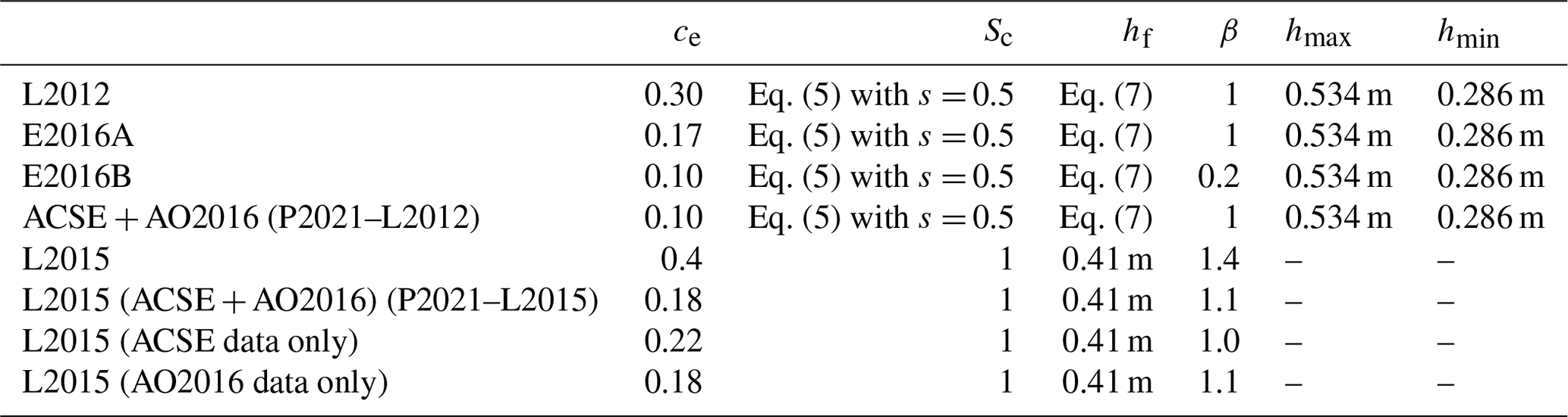
Table 1 Parameter settings for the form drag component of the L2012 scheme (Lüpkes et al., 2012, rows 1–4): as recommended in L2012, E2016A and E2016B, P2021–L2012; and the L2015 scheme (Lüpkes and Gryanik, 2015, rows 5–8): as recommended in L2015, and fit to ACSE + AO2016, ACSE only, AO2016 only. The L2012 variants use: D_min= 8 m and D_max= 300 m, whereas the L2015 variants use D_min= 300 m. The primary tuning parameter is the effective resistance coefficient, c_e, whereas β has a second-order effect on the shape of the curve. S_c and h_f were tunable parameters in L2012, but found by L2015 to have a marginal impact and set as constants for simplicity. P2021–L2015 is the proposed parameterization which is presented with L2015 anchored at the observed values of C_D10nw and C_D10ni.

3 Measurement and methods

3.1 Field measurements

We utilize data from two field campaigns, the Arctic Cloud in Summer Experiment (ACSE, Tjernström et al., 2015, 2019; Achtert et al., 2020), part of the Swedish–Russian–US Arctic Ocean Investigation on Climate-Cryosphere-Carbon (SWERUS-C3), and the Arctic-Ocean 2016 (AO2016) expedition. Both ACSE and AO2016 were carried out on board the Swedish icebreaker Oden. The ACSE cruise took place between 5 July and 5 October 2014, starting and ending in Tromsø, Norway, and working around the Siberian shelf, through the Kara, Laptev, East Siberian and Chukchi seas (Fig. 1). There was a change of crew and science team in Utqiaġvik (formerly Barrow), Alaska, on 20 August. The AO2016 expedition took place between 8 August and 19 September 2016 in the central Arctic Ocean, starting from, and returning to, Longyearbyen, Svalbard (Fig. 1).

3.2 Surface turbulence and meteorological measurements

Turbulent fluxes were measured with an eddy covariance system installed at the top of Oden's foremast, 20.3 m above the waterline. On ACSE this consisted of a Metek USA-100 sonic anemometer with heated sensing heads, a Li-COR Li-7500 open path gas analyser, and an Xsens MTi-700-G motion sensing package installed at the base of the anemometer. The ship's absolute heading and velocity were obtained from its navigation system. The Metek sonic anemometer failed at the start of AO2016 and was replaced with a Gill R3 sonic anemometer. The raw turbulent wind components, at 20 Hz, were corrected for platform motion following Edson et al. (1998) and Prytherch et al. (2015). Corrections for flow distortion of the mean wind were derived from a computational fluid dynamics model (Moat et al., 2015). Turbulent fluxes of heat, momentum and moisture were estimated by the eddy covariance technique over 30 min averaging intervals.

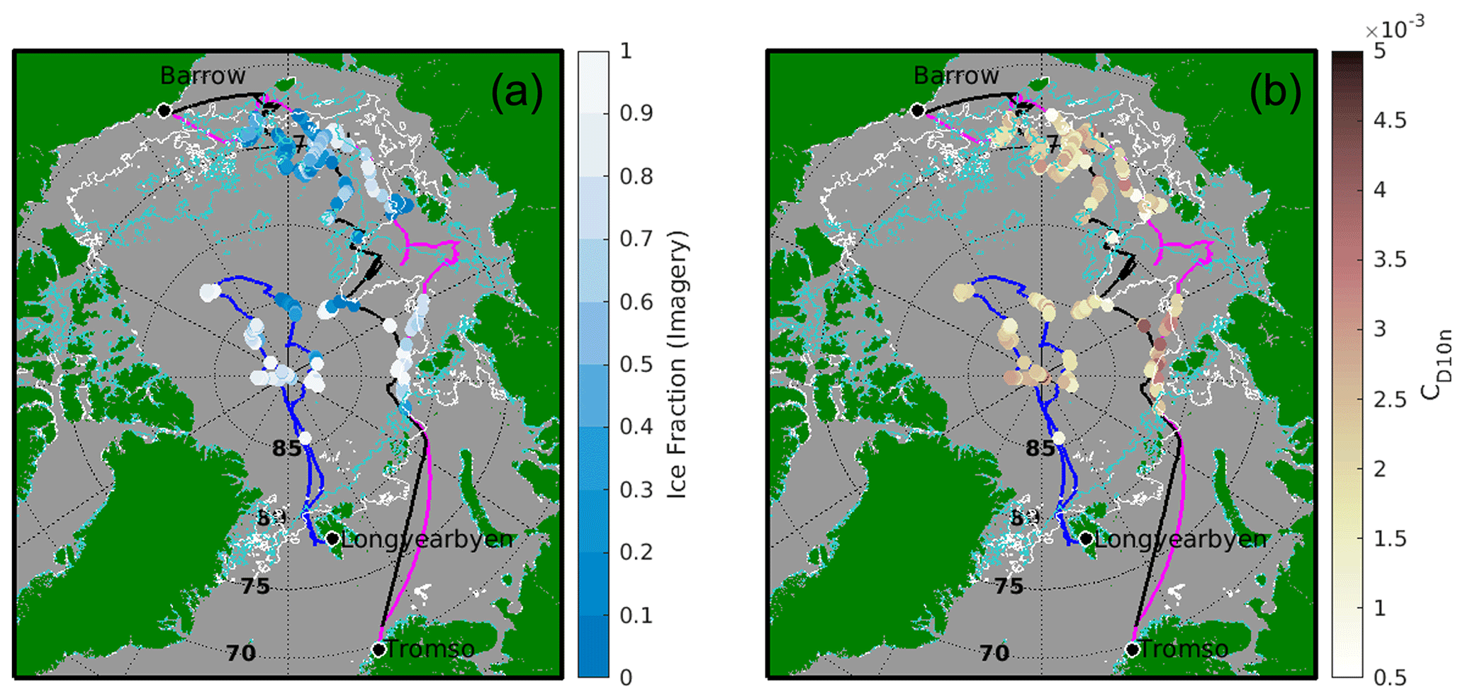
Figure 1 The cruise tracks of ACSE (leg 1, 5 July to 18 August 2014 (magenta) and leg 2, 21 August to 5 October (black)) and AO2016 (8 August to 19 September 2016, (blue)) with (a) sea-ice fraction from in situ imagery and (b) C_D10n, for each 30 min flux period shown. The sea-ice extent from AMSR2 on 7 August 2014 (white) and 2016 (cyan) – about midway through ACSE and at the start of AO2016 – are shown for reference and to give an indication of the variability between years.

Mean temperature (T) and relative humidity (RH) at the mast top were measured with an aspirated sensor – a Rotronic T $/$ RH sensor during ACSE and a Vaisala HMP-110 during AO2016. Additional T, RH and pressure (P) measurements were made by a Vaisala PTU300 sensor on the seventh deck of the ship. Pressure at the mast top was obtained by height-adjusting the measurement from the seventh deck. The surface skin temperature was obtained from two Heitronics KT15 infra-red surface temperature sensors, mounted above the bridge and viewing the surface on either side of the ship. Digital imagery of the surface around the ship was obtained from 2 Mobotix M24 IP cameras mounted on the port and starboard beam rails above the bridge, approximately 25 m above the surface. Images were recorded at 1 min intervals during ACSE and at 15 s intervals during AO2016. Profiles of atmospheric thermodynamic structure and winds were obtained from Vaisala RS92 radiosondes, launched every 6 h throughout both cruises. During ACSE a Radiometer Physics HATPRO scanning microwave radiometer provided additional retrievals of lower-atmosphere temperature profiles every 5 min.

3.3 Estimation of turbulence parameters and data screening

The transfer coefficient of momentum is computed as

$$\begin{array}{}\text{(12)}& C_{\mathrm{D}\mathrm{10}\mathrm{n}}={\left({\displaystyle \frac{u_{*}}{U_{\mathrm{10}\mathrm{n}}}}\right)}^{\mathrm{2}},\end{array}$$

where u_* is the measured friction velocity, and U_10n is the 10 m equivalent neutral wind speed corresponding to the 10 m wind speed U₁₀, and determined using Monin–Obukhov similarity theory and the Businger–Dyer stability correction function f_m (Businger et al., 1971) as U_10n=U₁₀f_m.

A total of 3421 and 1555 individual half-hourly flux estimates were obtained during ACSE and AO2016 respectively. Data were removed from the analysis if they failed a set of flux quality control criteria (Foken and Wichura, 1996) resulting in a subset of 1804 (247) flux estimates. Additional quality control criteria were applied to filter out data unreliable for analysis of transfer coefficients:

• The relative wind direction was restricted to ±120${}^{{}^{\circ }}$ from bow-on, where the flow is clear of the ship's superstructure.

• Data points where the stability parameter, $z/L$, was greater than 1 or less than −2 were removed to avoid the effects of strong stability and instability.

• Sign constancy between the turbulent heat flux and mean gradients was enforced. The Richardson number, Ri_B, and $z/L$ should always have the same sign, whereas the sensible heat flux, H, should have the opposite sign to $z/L$. Inconsistencies may arise owing to combined measurement uncertainties where the temperature gradient or H is small.

• Data were also removed where the 10 m wind speed was less than 3 m s⁻¹.

After initial quality control we have a total of 1403 and 162 half-hourly flux estimates. For ACSE data, an additional quality control criterion was applied based on the boundary-layer profiles. Working around the MIZ, ACSE experienced multiple warm air advection events. These result in strong near-surface air mass modification and the formation of very low or surface-based temperature inversions (Tjernström et al., 2019), which can exhibit significant spatial and temporal variability. Temperature profiles from the HATPRO microwave radiometer, bias-corrected through extensive comparisons with 6-hourly radiosondes, were used to detect surface inversions with 5 min temporal resolution following Tjernström et al. (2019). The profiles were classified as surface-based inversions, low-level inversions (inversion base height < 200 m), and well-mixed boundary layers (inversion base height > 200 m). The flux periods with mixed surface-based and low-level inversions were discarded from the analysis on the basis that the change in near-surface thermodynamic structure was likely to compromise the quality of the flux-profile relationship upon which the calculation of C_D10n depends. Following this step, we were left with 1051 data points from the ACSE campaign. No high-frequency profile measurements were available from AO2016; however, operating much further from the ice edge, AO2016 was not subject to the frequent warm air advection and air mass modification events seen during ACSE.

3.4 Determination of sea-ice concentration

Estimates of sea-ice fraction are drawn from two sources: (i) a local estimate of ice fraction determined from digital imagery from the ship; and (ii) daily ice fractions, derived from satellite-based Advanced Microwave Scanning Radiometer (AMSR2) passive microwave measurements (Spreen et al., 2008).

Our local raw imagery consists of high-definition (2048×1536) images of the surface to port and starboard, obtained from Mobotix MX-M24M IP cameras mounted above the ship's bridge, 25 m above the surface. Additional images from a camera pointed over the bow are used for visual inspection while selecting the periods when Oden was in the ice, but are not processed because the ship dominates the near field of the image.

On-board imagery can provide local surface properties including sea ice and melt pond fractions with a spatial resolution of order metres on a time base matched to the flux-averaging time (Weissling et al., 2009). The large volume of imagery sampled requires automated image-processing techniques to estimate ice properties (Perovich et al., 2002; Renner et al., 2014; Miao et al., 2015; Webster et al., 2015; Wright and Polashenski, 2018). Here we use the Open Source Sea-ice Processing (OSSP) algorithm of Wright and Polashenski (2018). The surface properties obtained during each 30 min interval are averaged to give the sea-ice and melt-pond fractions. The image processing methodology is described in Appendix A. Limitations on quality and availability of imagery resulted in a further 206 (36) flux estimates for the ACSE (AO2016) datasets being discarded. After all quality control criterion are applied and flux estimates matched with robust estimates of the local ice fraction, we retain a total of 542 flux estimates: 416 from ACSE and 126 from AO2016. Initially, melt ponds are treated as open water; the impact of this is examined in Appendix B.

The area of each image is approximately 34 225 m²; the total area imaged within each 30 min averaging interval varies with the number of images passing quality control, and the ship's movement, but is up to a maximum of approximately 2 km² during ACSE and 6.7 km² during AO2016.

Satellite-based sea-ice products are widely used to prescribe ice concentration in operational forecast models and have been used to assess the dependence of in situ flux measurements as a function of ice fraction (e.g. Prytherch et al., 2017). However, they have significant uncertainties when related to in situ flux measurements due to their relatively coarse temporal and spatial resolution (Weissling et al., 2009), resulting in a mismatch between the satellite footprint and that of the surface flux measurement, and the times of the measurements. The AMSR2 satellite measurements used here provide daily sea-ice concentration on a 6.25 km grid, whereas eddy covariance flux estimates are for 30 min periods and have a footprint of the order of a few hundred metres to a kilometre. The AMSR2 estimates are interpolated spatially to the locations of each flux measurement.

4 Results

4.1 Atmospheric conditions during ACSE and AO2016

Figures 2 and 3 show the meteorological and surface conditions during ACSE and AO2016. The first half of ACSE was dominated by relatively low winds, and surface temperatures close to 0 ^∘C when in the ice; much warmer temperatures are associated with open coastal waters. The second half of the cruise experienced higher, and more variable winds, associated with multiple low-pressure systems. Temperatures first fell to the freezing point of salt water on day of year (DoY) 218, although Sotiropoulou et al. (2016) identified the start of freeze up as DoY 241. AO2016 saw a shift from relatively low surface air pressure, and mostly low winds to higher pressure and more variable winds with frequent occurrence of high winds around DoY 237.

Out of the total of 542 flux estimates, we have 184, 282 and 76 flux estimates in stable ($z/L$ > 0.01), near-neutral (−0.01 < $z/L$ < 0.01) and unstable conditions ($z/L$ < −0.01) respectively. This distribution in static stability augments the limited datasets already available over the marginal ice zone, which have been predominantly in unstable conditions (e.g. E2016).

4.2 Ice surface characteristics

Figure 4 shows the variation over time of the ice, melt-pond, and open-water fractions determined from the on-board imagery and from AMSR2. Note that the variations represent geographic variability along the cruise tracks, as well as temporal changes in ice conditions. During the early phase of the ACSE campaign, to mid-July (DoY 185 to 196), the ice encountered was mostly old ice (Tjernström et al., 2019), with an average ice concentration of about 70 %; melt ponds and open water had 11 % and 18 % coverage respectively. In this phase the average concentration from AMSR2 was 95 % – larger than the sum of average local ice and melt-pond concentrations (81 %). From late July to early August (DoY 209 to 229), the average local ice concentration was 56 %, with melt-pond and open-water fractions of about 17 % and 27 %. Here the AMSR2 concentration was lower than that from imagery, at 44 %.

Figure 2 Time series of (a) 10 m neutral wind speed, U_10n and surface pressure, P_surf, (secondary axis), (b) friction velocity, u_* (c) surface temperature, T_surf and relative humidity, RH, (secondary axis), (d) air temperature, T_air, (e) 10 m equivalent neutral drag coefficient, C_D10n, (f) ice fraction from AMSR2 satellite, (g) Monin–Obukhov stability parameter, $z/L$, for $z/L$ > 0 (stable) and (h) $z/L$ < 0 (unstable), for ACSE data. The grey dots are 30 min flux periods from the whole cruise, whereas the black dots correspond to the flux data points that pass quality control. In panels (c) and (d), the dashed red lines show $T_{\mathrm{air}}=T_{\mathrm{surf}}=$ 0 ^∘C.

Figure 3 As Fig. 2 but for AO2016.

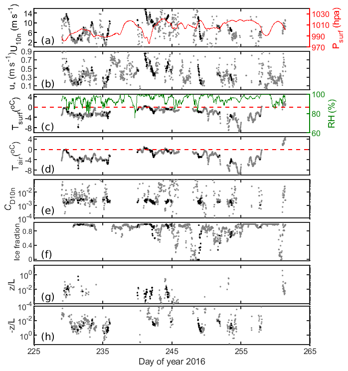
During this period, warm continental air from Siberia flowed northward across the Oden's track causing a rapid melting of ice (Tjernström et al., 2015, 2019). From late August to mid-September (DoY 239 to 255), the average local concentration declined to 27.6 % and the surface was mostly characterized by large areas of open water (63 %). The AMSR2 ice fraction was 54 %, approximately twice that from the imagery. During late September (DoY 268 to 272), a large variation in the surface conditions was observed and often the ice concentration was higher than 90 % owing to the presence of newly formed thin ice, nilas and pancake ice. During the AO2016 campaign, the surface was mostly characterized by old and thick ice, with intermittent patches of thin ice and melt ponds, reflecting the more northerly cruise location. The average ice concentrations from imagery and AMSR2 were found to be about 80 % and 90 % respectively.

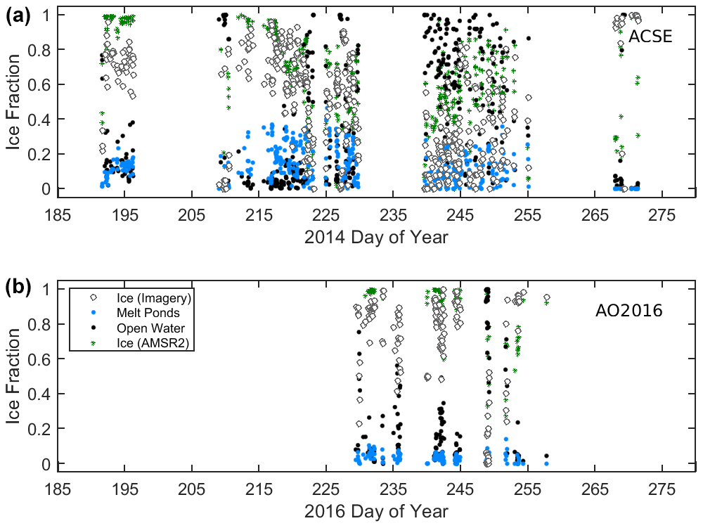
Figure 4 Time series of ice, melt-pond and open-water fractions (white, blue and black symbols respectively) from the local imagery, and ice fraction (green) from AMSR2, interpolated to the ship location. (a) is for ACSE and (b) for AO2016.

Figure 5 shows a direct comparison of the ice fraction from the in situ imagery and AMSR2. There is a broad correspondence, but a very high degree of scatter, and AMSR2 tends to overestimate the local sea-ice fraction; the correlation coefficient, mean absolute bias and root-mean-square error are 0.64, 0.21 and 0.28 respectively. It is clear from the ice concentration time series, however, that the bias between AMSR2 and the local ice fraction varies over time and appears to be related to the surface conditions of melt or freeze up, in particular when changes are rapid. The largest difference between ice fractions from both projects was found during the early freeze-up season where there is extensive very thin ice.

Figure 5 A comparison of the ice fraction derived from the local imagery and from AMSR2 for both field campaigns. The linear regression (A_AMSR= 0.584A_Img+ 0.321) and 1:1 lines are shown in blue and black respectively.

4.3 Variation of momentum transfer coefficient with sea-ice concentration

We first assess the variability of surface drag with the sea-ice fraction using local ice concentration from the onboard imagery (Fig. 6). The range and median values of C_D10nover sea ice (A_Img > 0) are similar to those of previous studies (Banke and Smith, 1971; Overland et al., 1985; Guest and Davidson, 1987; Castellani et al., 2014; E2016). The peak C_D10n is found at the 0.6–0.8 ice-fraction bin, consistent with L2012 and E2016). The median values of C_D10n in both datasets agree well for high ice fractions (Fig. 6b and c); however, there are insufficient AO2016 data for A_Img < 0.5 to make a robust comparison with ACSE. Given the good general agreement between ACSE and AO2016, we will only consider the joint dataset from here on.

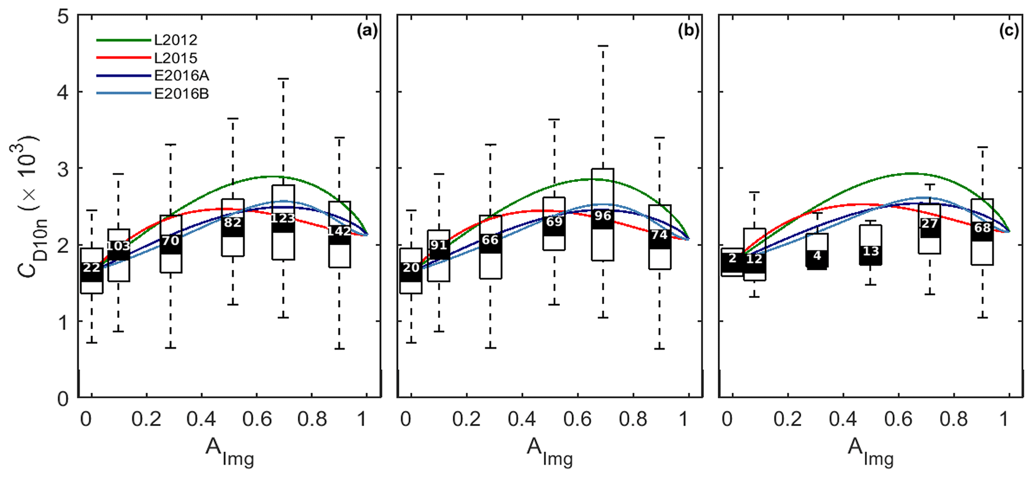
Figure 6 C_D10n as a function of ice fraction, as derived from local imagery (A_Img) for (a) the joint ACSE and AO2016 datasets (n= 542), (b) the ACSE dataset (n= 416) and (c) the AO2016 dataset (n= 126). The boxes show the interquartile range and the bin median (black squares) for bins of width = 0.2 and plotted at the mean ice fraction for the bin; the number of data points in each bin is noted at the median level. Whiskers indicate the range of the estimates, excluding any outliers, which are plotted individually if present. Parameterization schemes are overlain as indicated, with each curve anchored at the observed median values of C_D10nw (A_Img= 0) and C_D10ni (defined here as A_Img > 0.8) for each dataset.

The measurements are compared with the L2012, L2015 and E2016 parameterization schemes. Note that these all require specified values of C_D10n over open water (A_Img= 0) and solid ice (A_Img= 1) (see Eq. 2); these vary with conditions, dramatically so for A_Img= 1, as demonstrated by E2016. Here, we follow E2016 and fix the values of C_D10nw and C_D10ni used in the parameterizations to the measurements, using the observed median values at A_Img= 0 and A_Img > 0.8 respectively for each dataset. Note that A > 0.8 is used, as opposed to A= 1, as navigational consideration meant that the ship rarely operated in regions with an ice fraction of 1. The mean ice fraction in this bin is 0.89. Here, we do not adjust any of the other tuneable parameters in these parameterizations.

L2012 overestimates the observations of all but the lowest ice concentrations. E2016a and E2016b – which follow L2012 with settings tuned to measurements over the MIZ from Fram Strait and the Barents Sea – correspond well with the observations, with only a slight overestimation of the peak values. L2015, which accounts for form drag over water as well as over ice, is a close match to the observations for A_Img > 0.6 but overestimates the 0.2–0.4 and 0.4–0.6 bins and peaks at too low an ice concentration. Note that we will tune the L2015 scheme using our measurements in Sect. 4.4.

The median value of C_D10n at A= 0 was $\mathrm{1.65}\times {\mathrm{10}}^{-\mathrm{3}}$, which is higher than those typically found over the open ocean (Smith, 1980; Large and Yeager, 2009). This may be a result of the open water measurements being made under fetch-limited conditions close to the ice edge, or within regions of open water within the pack ice, where an under-developed wave state may result in higher drag (Drennan et al., 2003). We cannot, however, exclude the possibility that they result from an incomplete correction for flow distortion over the ship (Yelland et al., 1998, 2002), or that the flux footprint includes flow over nearby ice that is not visible in the imagery.

Figure 7 shows C_D10n as a function of the AMSR2 ice fraction. There is broad agreement with the values in Fig. 6a at low and high ice concentrations, but there is no peak in C_D10n at intermediate concentrations. Instead, the measurements with higher drags have moved to either lower or higher ice fraction bins. This is consistent with neither our in situ imagery nor previous aircraft-based studies, suggesting that it might be a limitation of the AMSR2 imagery.

Figure 7 As Fig. 6a but for the ice fraction derived from the AMSR2 satellite.

4.4 Updating parameterizations using local sea-ice concentration measurements

L2015 extended the parameterization of L2012 to explicitly represent the impact of fetch dependence over heterogeneous surfaces in a physically consistent manner. To date, this scheme has been unconstrained by observational data. Here, we validate the scheme and provide recommendations for its tuneable parameters based on the joint ACSE and AO2016 datasets. E2016 pointed out that variation in the morphological parameters β and c_e in L2012 could explain the variability of C_D10n within concentration bins. Reducing the values of β and c_e from those suggested by L2012 resulted in a better fit to their data.

In the fetch-dependent L2015 parameterization, increasing β (sea-ice morphology exponent, Eqs. 8 and 9) results in decreasing C_D10n, mostly at high ice concentrations, whereas increasing c_e (the effective resistance coefficient) increases C_D10n at all concentrations. Here we have adjusted the L2015 values of β and c_e to optimize the fit to our measurements. The revised values of the coefficients are given in Table 1. For a consistent comparison, similar tuning is applied to L2012.

Figure 8 shows C_D10n plotted against A_Img along with the tuned L2015 and L2012 schemes, both anchored to the observed values of C_D10n at A_Img= 0 and A_Img > 0.8 for the joint dataset.

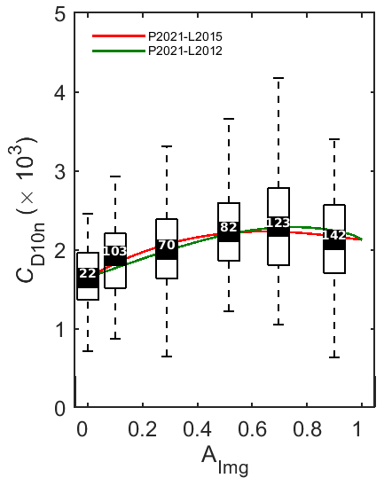
Figure 8 C_D10n as a function of the local ice fraction (A_Img) for the joint ACSE and AO2016 (n= 542) dataset. Here, the proposed parameterization (red line, P2021–L2015) is presented with L2015 anchored at the observed values of C_D10nw (A_Img= 0) and C_D10ni(A_Img > 0.8) with the coefficients β and c_e shown in Table 1. For comparison, the L2012 scheme (green line, P2021–L2012) is also tuned with the curve anchored at the same values of C_D10ni and C_D10nw with β and c_e shown in Table 1.

Both L2012 and L2015 provide an excellent fit to the data, passing close to the median observed values at all ice fractions. The fitted curve for the joint dataset (P2021–L2015) works equally well for the individual datasets (Fig. S1, Supplement).

In the analysis above we have considered C_D10n as a function of ice fraction – no distinction is made between melt ponds and open water. However, there are uncertainties in the surface classification, in particular for the determination of melt-pond fraction. Thin ice and shallow melt ponds can appear very similar in colour, and potentially be misclassified by the image-processing algorithm. An assessment of the sensitivity of the fitting of the L2015 to the presence and treatment of melt ponds (see Appendix B) shows that they have little impact.

Melt ponds are explicitly included in the L2012 and L2015 parameterizations in their more complex levels of implementation, where the edges of melt ponds provide a source of form drag. Tsamados et al. (2014) modelled the different contributions to the total drag using L2012 implemented within the CICE sea ice model (Hunke and Lipscomb, 2010). They found that melt ponds made a negligible contribution to the drag except over the oldest, thickest ice just north of the Canadian archipelago, consistent with our observations.

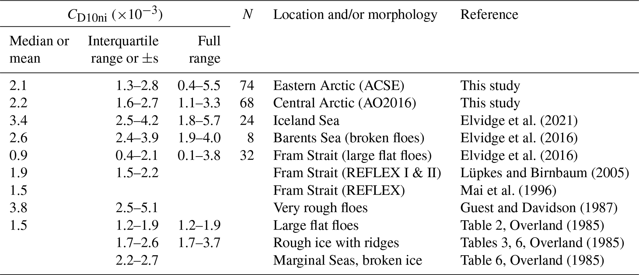
Both L2012 and L2015 can be tuned to provide excellent fits to the observations (Fig. 8). Even without tuning to this dataset, the differences between L2015, E2016A and E2016B are modest and all lie within the interquartile range of the observed C_D10n at all ice fractions (Fig. 6a). The largest source of uncertainty in the application of these schemes is the value of the drag coefficient at 100 % ice fraction, C_D10ni, which must be prescribed, and is strongly dependent on ice morphology. Table 2 lists values of the neutral drag coefficient for very high ice fractions (0.8–1 from this study, and 0.9–1 or 1 in previous studies) reported in the literature. The best estimates (mean or median values) vary by a factor of more than 4. As discussed in previous studies, C_D10ni depends on the sea-ice morphology and so prescribing this as one value is a drastic simplification.

Table 2 Overview of neutral drag coefficients based on in situ eddy covariance measurements over “complete” sea-ice cover (C_D10ni) from this and previous studies. The values are taken from the literature, and so vary as to whether the mean, median or a range of values is shown. The definition of “complete” sea ice covers a range of ice fractions (0.8–1, 0.9–1.0, and exactly 1) depending on the study. N is the number of data points in this bin where specified. The 2nd column provides the interquartile range or the range from −1 to +1 s, where s is the standard deviation. Note Guest and Davidson (1987) uses the turbulence dissipation method. Overland (1985) compiles values from a variety of previous studies in various locations, as well as new data; thus, the values reproduced here are a compilation by morphology.

5 Conclusions

An extensive set of measurements of drag coefficients over sea ice, obtained during two research cruises within the Arctic Ocean, has been utilized to evaluate the dependence of drag on the ice fraction. The final dataset consists of 542 estimates of drag coefficients along with estimates of the local ice fraction obtained from high-resolution imagery of the surface around the ship. The measurements cover a wide geographic area, summer melt and early autumn freeze up, and a range of surface conditions from thick multiyear ice, through melting ice with melt ponds, to newly formed thin and pancake ice, and near-surface stability conditions of −2 < $z/L$ < 1, a much wider range than E2016. This wide range of conditions means that the results should be broadly representative of much of the Arctic sea ice region.

The dependence of C_D10n on the ice fraction is evaluated in the context of state-of-the-art parameterization schemes (Lüpkes et al., 2012; Lüpkes and Gryanik, 2015). The most recent of these (Lüpkes and Gryanik, 2015) attempts to account for the impact of short fetch over ice/water over spatially highly heterogeneous surfaces. When tuned to the observations, the parameterizations provide an excellent representation of C_D10n as a function of ice fraction:

The main conclusions are

• The data support the existence of a negatively skewed distribution of C_D10n with ice concentration, with a peak value for fractions of 0.6–0.8, consistent with the predicted behaviour from Lüpkes et al. (2012) and observations of Elvidge et al. (2016).

• When tuned to our measurements, both L2012 and L2015 provide an excellent fit to the observed variation of C_D10n with the ice fraction. The impact of small-scale surface heterogeneity and the influence of fetch is likely to increase with increasing contrast in the skin temperatures of the ice and water surfaces, and thus play a greater role in the winter.

• Melt ponds had no significant impact on the drag coefficient over the study area. The optimal fit of the L2015 parameterization to the measurements had little sensitivity to the uncertainty in partitioning of melt ponds to the ice or water fractions when estimating the local ice fraction, and there was little sensitivity to the presence of melt ponds at all for the conditions observed.

• When evaluated against the AMSR2 retrieval of the ice fraction, the behaviour of C_D10n is not consistent with in situ observations, for example, no peak is seen at intermediate ice fractions. This is likely a result of several factors: a mismatch in the spatial scale between the in situ flux footprint (of order 100 s of metres to 1 km) and the satellite footprint (6.5 km); potential spatial offsets in location matching resulting from the low temporal resolution of the satellite data (daily retrievals) combined with drifting of the ice; and the high scatter and varying mean bias between the in situ and satellite estimates of the ice fraction. The mean bias in particular displays temporal and spatial coherence that suggests a dependence upon surface conditions. This finding cautions against the use of comparatively low-resolution remote-sensing products when evaluating parameterizations.

Atmospheric stability may also play a role here, as it will affect how rapidly the atmospheric surface layer adjusts to changes in surface properties. L2015 incorporates stability effects at the higher levels of parameterization complexity, but not within the simplest complexity level used here. A much larger dataset, including the details of surface heterogeneity, would be required to evaluate the details of both stability and fetch dependencies.

Sea ice and climate models are starting to incorporate components of form drag within their surface exchange schemes for sea ice (e.g. Tsamados et al., 2014; Renfrew et al., 2019). But at present, most do not use all the components of the more complex versions of schemes such as L2012 or L2015. Instead, they tend to rely on the simplest versions where drag is only a function of the ice fraction. In operational forecast models, where only a prescribed ice concentration from a satellite retrieval may be available, this seems appropriate, but within more complex coupled weather and climate prediction models there is the potential for using output from the sea-ice model to adjust the drag coefficient (E2016; Renfrew et al., 2019). The skill of parameterization is strongly dependent on the accurate representation of the drag at 100 % ice fraction, C_D10ni, which varies significantly with ice morphology (Lüpkes et al., 2012; Lüpkes and Gryanik, 2015; Elvidge et al., 2016, 2021). Tackling the representation of C_D10ni should be the next challenge in improving air-ice surface drag in weather and climate models.

Appendix A: Image processing and evaluation of the local ice fraction

A total of ∼500 000 images of the surface around the ship were obtained over the two cruises; thus, this required an automated approach to estimating the local ice fraction. Here we use the Open Source Sea-ice Processing (OSSP) algorithm of Wright and Polashenski (2018).

A1 (a) Pre-processing

Of the images available for each flux period, a subset of visibly good images was selected for further processing. The rejection of images was due to the presence of dense fog, moisture or ice on the camera lens, strong surface reflection of direct sunlight, or insufficient illumination. The selected subsets consist of 10 to 60 images in each flux period (e.g. Fig. A1a). These images are first corrected for lens distortion. The lens-specific distortion coefficients and intrinsic parameters were determined using the Computer Vision System Toolbox of MATLAB. The corrected images (2048×1536 pixels) were then cropped to select a region within ∼200 m of the ship (2009×1111 pixels) – e.g. see Fig. A1b.

A2 (b) Training and implementation of the algorithm

The success of any machine learning-based algorithm depends upon the quality of the training dataset. As the ice conditions varied substantially throughout the campaigns, extensive training data were needed to cover the wide range of conditions. The initial training images selected were from the first and last images from each flux period. Additional images were added iteratively depending upon the performance of the algorithm on randomly selected images. After multiple trials, we settled on three different training datasets for (i) images with a visibly large ice fraction, (ii) images with a large open water fraction and (iii) images showing newly formed thin ice. Our approach was to generate a training dataset that could be utilized equally on imagery from other campaigns, while keeping the number of discrete training datasets as small as possible. The training data, identifying ice, water and melt-ponds, were generated based on user classification of the training images via a Graphical User Interface (GUI), and thus depends upon the ability of the user to identify the surface features correctly.

A3 (c) Post-processing

The OSSP algorithm produces an indexed image having pixel-wise information about surface features (open water, melt ponds, ice) for each input image (e.g. Fig. A1c). As the images were necessarily taken at an oblique angle, the indexed images need to be orthorectified to derive the correct fractions of ice, melt pond and water. Orthorectification of imagery is a process by which pixel elements of an oblique image are restored to their true vertical perspective position. The angular separation of each

pixel (after correction for lens distortion) was determined from a laboratory calibration of the cameras. The angle from the horizon (the horizontal) in the images and the height of the camera above the surface then allow the location of each pixel on the surface to be calculated. The masked images were interpolated onto a regular x–y grid after orthorectification and area fractions of ice and melt ponds were estimated as a fraction of the total number of pixels for each category (e.g. Fig. A1d). The average fractions of ice and water for a flux period are then calculated by taking an average over all the images in that period. Only flux periods having more than 30 available images are included in the analysis.

Each orthorectified image has an area of approximately 34 225 m²; the total area included in each 30 min average varies with ship manoeuvres and the number of images passing quality control. With a maximum in-ice ship speed of 5 m s⁻¹, the 1 min images from ACSE do not overlap, providing a maximum area of 2.05 km⁻². For the 15 s imagery during AO2016, images overlap by 75 m at a ship speed of 5 m s⁻¹, giving a maximum area of approximately 6.7 km⁻². It is implicitly assumed that the ice fraction determined along the ship track is representative of that within the flux footprint, i.e. that the ice structure is more or less homogeneous within the footprint.

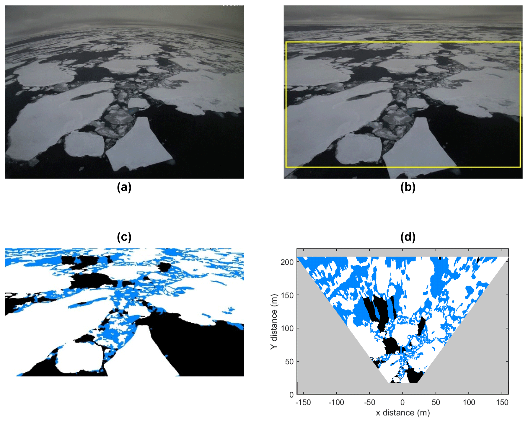
Figure A1 An example of the image processing workflow. Panel (a) is an example raw image; (b) shows the image corrected for the lens distortion, where the region of focus is shown by the yellow rectangle; (c) shows the image after processing by the OSSP algorithm where the masking colours – white, blue and black – represent ice, melt pond or submerged ice and open water areas respectively; (d) shows the orthorectified image showing the true distance of each surface feature away from the camera.

Appendix B: Sensitivity to melt ponds

Here we investigate the sensitivity of our tuning of L2015 to the melt pond fraction. We reclassify 50 % and 100 % of melt ponds as ice instead of water (Fig. B1) and the L2015 function is re-fitted to the revised ice fractions and compared with our original fit.

The reclassification of melt ponds as ice has the effect of moving some drag estimates into higher ice fraction bins, slightly increasing the median value of C_D10n at high ice fractions. The refitted L2015 functions reflect this slightly higher drag at high ice fraction but are essentially unchanged for A < 0.5. Note that even when A > 0.5 the change in the L2015 functions is very small compared with the variation in C_D10n within each ice concentration bin. We further investigate the sensitivity of the parameterization to the presence of melt ponds by a simple sub-setting of the data by the melt-pond fraction. In all cases the melt-pond fraction is < 0.6. Figure B2 shows C_D10n with the ice fraction for cases where the melt-pond fraction is <  0.3 (Fig. B2a) and < 0.1 (Fig. B2b). The L2015 function is fitted to these subsets of data and compared with that of the full dataset. The revised fits differ negligibly from that of the full dataset, suggesting that C_D10n might not be strongly dependent on the extent of melt ponds. In short, the sensitivity of the parameterization to the treatment of melt ponds is negligible.

Figure B1 Parameterization sensitivity to the melt-pond (MP) fraction. Panel (a) re-classifies half of melt ponds to sea ice (A' = A + 0.5 ⋅ MP), whereas (b) re-classifies all of the melt points to sea ice (A' = A + MP), where A is the sea-ice fraction. The curves show the L2015 parameterization, tuned to the original ice fraction observations (red; P2021–L2015) and tuned to the adjusted ice fraction observations (black).

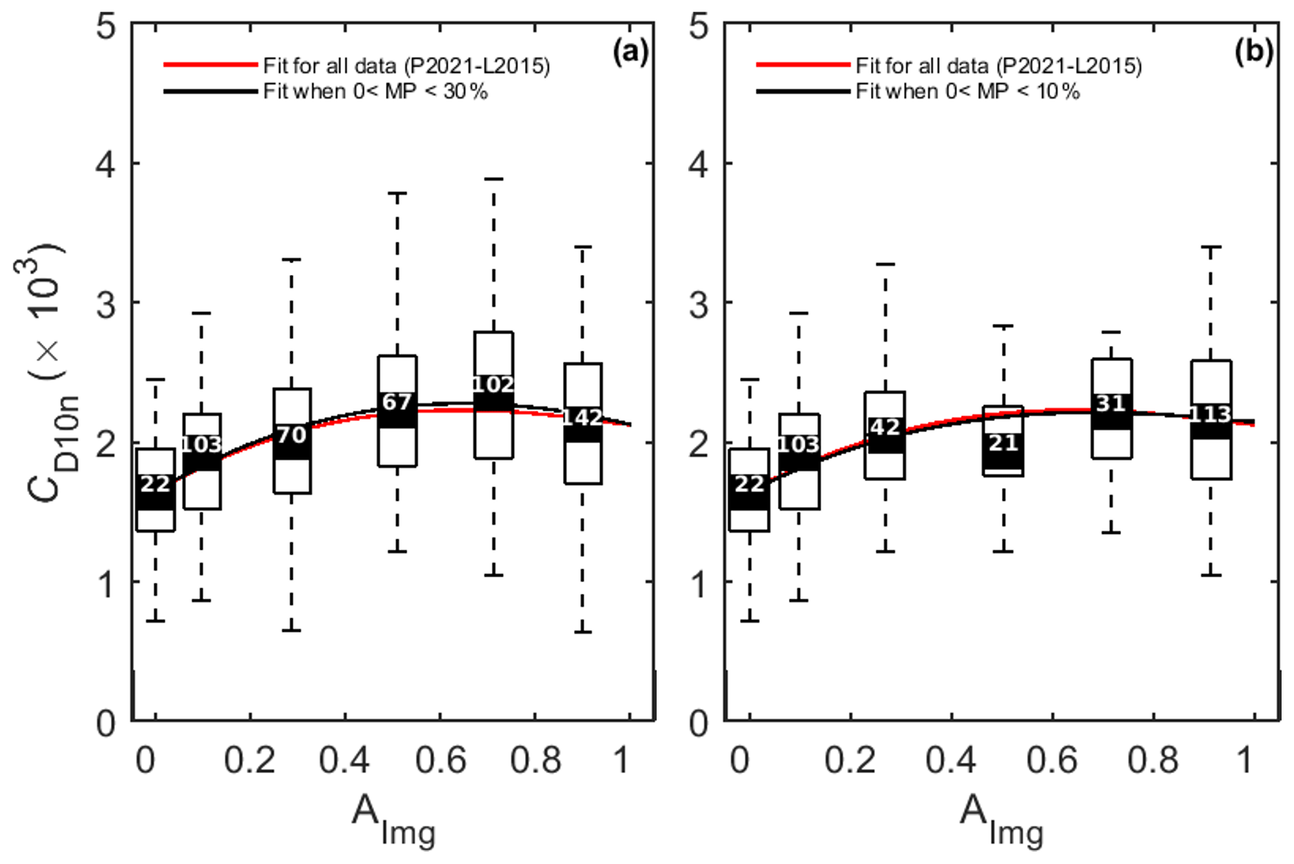
Figure B2 (a) MP < 30 % (b) MP < 10 %. In each panel, the red curve is the fitting curve obtained for the joint ACSE and AO2016 data, the same as shown in Fig. 8 (P2021–L2015), and the black lines are the fitting curve obtained for the data shown in the “respective” panels.