Exploiting satellite measurements to explore uncertainties in UK bottom-up NO_x emission estimates

Nitrogen oxides (NO_x, NO + NO₂) are potent air pollutants which directly impact on human health and which aid the formation of other hazardous pollutants such as ozone (O₃) and particulate matter. In this study, we use satellite tropospheric column nitrogen dioxide (TCNO₂) data to evaluate the spatiotemporal variability and magnitude of the United Kingdom (UK) bottom-up National Atmospheric Emissions Inventory (NAEI) NO_x emissions. Although emissions and TCNO₂ represent different quantities, for UK city sources we find a spatial correlation of ∼0.5 between the NAEI NO_x emissions and TCNO₂ from the high-spatial-resolution TROPOspheric Monitoring Instrument (TROPOMI), suggesting a good spatial distribution of emission sources in the inventory. Between 2005 and 2015, the NAEI total UK NO_x emissions and long-term TCNO₂ record from the Ozone Monitoring Instrument (OMI), averaged over England, show annually decreasing trends of 4.4 % and 2.2 %, respectively. Top-down NO_x emissions were derived in this study by applying a simple mass balance approach to TROPOMI-observed downwind NO₂ plumes from city sources. Overall, these top-down estimates were consistent with the NAEI, but for larger cities such as London and Birmingham the inventory is significantly (>25 %) less than the top-down emissions.

1 Introduction

Poor air quality (AQ) can have a substantial impact on human health, increasing risk of ailments such as asthma, cancer, diabetes and heart disease (Royal College of Physicians, 2016). A key air pollutant is nitrogen dioxide (NO₂), which was responsible for approximately 9600 premature deaths from long-term exposure in the United Kingdom (UK) in 2015 (EEA, 2018). NO₂ is also a precursor to tropospheric ozone and nitrate aerosol in the UK (DEFRA, 2018a). Legislation (e.g. the EU directive 2008/50/EC Ambient AQ regulation; DEFRA, 2018a) is in place to reduce concentrations of NO₂ and other pollutants. However, many regions in the UK (33 out of 43 in 2019; DEFRA, 2020) still fail to meet the annual mean NO₂ limit of 40 µg m⁻³ (WHO, 2018). To meet the UK's statutory reporting requirements and to help inform policy, the Department for Environment, Food and Rural Affairs (DEFRA) uses the National Atmospheric Emissions Inventory (NAEI) (NAEI, 2021a). However, like all emission inventories, the NAEI is subject to uncertainties which are difficult to quantify. These uncertainties include unreported sources, diffuse sources such as agriculture, and the use of proxy data (e.g. population or housing density data) to distribute emissions and updates to the NAEI methodologies between years (NAEI, 2017). In addition, the NAEI only includes emissions from anthropogenic sources. Spatial verification of the NAEI AQ emissions, until recently (Tsagatakis et al., 2021), has been restricted to comparisons with surface sites, which have limited and disproportional spatial coverage. The NAEI is also used to drive regional models (e.g. the UK Met Office Air Quality in the Unified Model (AQUM, Savage et al., 2013), which provides the official national AQ forecasts), land use regression models (e.g. Wu et al., 2017), and pollutant climate mapping (PCM) models (e.g. Dibbens and Clemens, 2015), where uncertainties in the emissions can then feed into the simulated AQ predictions and resultant public health advisories.

Satellite measurements of tropospheric column NO₂ (TCNO₂) have frequently been used to derive top-down emissions of nitrogen oxides (NO_x=nitric oxide (NO) + NO₂), which can be used to evaluate bottom-up inventories. Some studies have used statistical fitting of observed downwind plumes of TCNO₂ from anthropogenic sources (e.g. Beirle et al., 2011; Liu et al., 2016; Verstraeten et al., 2018), while others have used complex atmospheric chemistry models deploying approaches such as data assimilation (e.g. Miyazaki et al., 2016), mass balance (Martin et al., 2003), and model sensitivity experiments (e.g. Potts et al., 2021).

While model-derived estimates of NO_x emissions (e.g. from data assimilation) are robust, the methodology is computationally expensive and time-intensive. Therefore, the statistical fitting to downwind plumes approach is a more achievable approach to derive top-down emissions, especially for government departments and agencies. Beirle et al. (2011) presented one of the first studies to use statistical fitting to downwind plumes for Riyadh, Saudi Arabia. The method was also applied to multiple megacities and compared with the bottom-up Environmental Database for Global Atmospheric Research (EDGAR) emission inventory (version 4.1). Verstraeten et al. (2018) used a similar, but modified, approach of simple mass balance which assumes that the observed total mass of NO₂ is a product of the emission rate and the effective lifetime. The assumption is that the removal of NO₂ can be described by a first-order loss (i.e. the chemical decay of NO₂ follows an exponential decay function with an e-folding time and therefore distance from the source).

In this study, we use satellite TCNO₂ records to evaluate the spatial distribution and temporal evolution of the NAEI. In the past, and still presently, this is a challenge given the climatological meteorological conditions (i.e. frequent frontal systems with widespread precipitation and cloud cover; Pena-Angulo et al., 2020) experienced in the UK. Frequent cloud cover means that satellite instruments are severely restricted in their ability to retrieve information on trace gases and aerosols through the atmosphere (i.e. retrievals only between the top of atmosphere and cloud top). Therefore, the lack of robust observations makes it more difficult to clearly resolve large emission sources from space. Also, previous sensors (e.g. the Ozone Monitoring Instrument, OMI) have had relatively coarse horizontal spatial resolutions (in the order of 10–100 km) which are larger than most UK emissions sources. However, this work represents the first attempt to derive UK city-scale NO_x emissions from the new state-of-the-art TROPOspheric Monitoring Instrument (TROPOMI), which has unparalleled spatial resolution in comparison to previous sensors (e.g. OMI). We apply a similar approach to Verstraeten et al. (2018) but determine the background NO₂ value and e-folding distance in different ways to derive top-down NO_x emission estimates of UK cities and thereby directly evaluate the NAEI estimates. Therefore, we can derive NO_x emissions from previously undetectable sources (e.g. Manchester and Birmingham). From here on, we refer to this methodology as the simple mass balance approach (SMBA). The satellite observations used, NAEI and SMBA, are described in Sect. 2, the results presented in Sect. 3, and our conclusions discussed in Sect. 4.

2 Data and methods

2.1 NAEI emissions

The NAEI is the official UK bottom-up inventory of primary sources of emissions, used for statutory reporting and national air quality policy and driving regional air quality models (NAEI, 2021a). The contract to deliver the NAEI is led by a consortium managed by Ricardo Energy and Environment for the UK Department for Business, Energy and Industrial Strategy (BEIS) and DEFRA. The NAEI is compiled on an annual basis according to internationally agreed methodologies (EMEP/EEA, 2019), encompassing sectors ranging from transport and industry through to agriculture and domestic sources (Ricardo Energy and Environment, 2021). Here, we use the NAEI emissions from 2019, which is the most recent version publicly available.

2.2 Satellite data

OMI and TROPOMI are both nadir-viewing instruments on board the NASA Aura and ESA Sentinel 5 – Precursor (S5P) polar-orbiting satellites, respectively, and have local overpass times of 13:30 local time (LT). TROPOMI measures in the ultraviolet-visible (UV-Vis, 270–500 nm), similarly to OMI (Boersma et al., 2007), as well as near-infrared (NIR, 675–775 nm) and short-wave infrared (SWIR, 2305–2385 nm) spectral ranges (Veefkind et al., 2012). TROPOMI and OMI have nadir pixel sizes of 3.5 km × 5.5 km (in the UV-Vis, 7.0 km × 7.0 km for other spectral ranges) and 13 km × 24 km, respectively. The OMI (DOMINO version 2 product) and TROPOMI (TM5-MP-DOMINO version 1.2/3x – OFFLINE product) data were downloaded from the Tropospheric Emissions Monitoring Internet Service (TEMIS) for January 2005 to December 2015 and February 2018 to January 2020, respectively. Given the issues with large cloud cover in the UK, we use 2 years of TROPOMI TCNO₂ data to help increase the spatiotemporal sample size when deriving top-down emissions to evaluate the 2019 NAEI NO_x emissions. The OMI row anomaly first occurred in 2008 (Torres et al., 2018) and over time has progressively had a detrimental impact on retrieved TCNO₂. The study by Pope et al. (2018) successfully used the OMI record to look at long-term trends in UK TCNO₂. However, after 2015, while still retrieving robust signals over source regions, the row anomaly appears to be substantially artificially enhancing background TCNO₂. Therefore, as we consider regional trends in TCNO₂ in Sect. 3.2, we did not use OMI TCNO₂ after 2015. The data have been processed using the methodology of Pope et al. (2018) to map the TCNO₂ data onto a high-resolution spatial grid (0.025^∘ × 0.025^∘, ∼2–3 km $\times \sim \mathrm{2}$–3 km for TROPOMI, $\mathrm{0.05}{}^{\circ }\times \mathrm{0.05}{}^{\circ }$, ∼5 km $\times \sim \mathrm{5}$ km for OMI). The TROPOMI data were quality controlled for a cloud radiance fraction <0.5, a quality control flag >0.75, and where the TCNO₂ value was $>-\mathrm{1.0}\times {\mathrm{10}}^{-\mathrm{5}}$ mol m⁻² (i.e. random values round 0.0 may be slightly negative or positive, so we filter for TCNO${}_{\mathrm{2}}>-\mathrm{1.0}\times {\mathrm{10}}^{-\mathrm{5}}$ mol m⁻²; otherwise, a positive bias in average TCNO₂ is imposed). While TROPOMI provides the greatest spatial resolution of any satellite instrument to measure air pollutants, suitable for deriving TCNO₂ emission estimates over UK city-scale sources, the retrieved TCNO₂ has been shown to have a low bias. Over north-western Europe, Verhoelst et al. (2021) found that TROPOMI underestimated TCNO₂ by approximately 20 %–30 % when compared with surface TCNO₂ measurements, which is consistent with Chan et al. (2020) and Dimitropoulou et al. (2020). OMI data were processed for a geometric cloud fraction of <0.2, quality flag =0 (which also flags pixels influenced by the row anomaly; Braak, 2010), and TCNO${}_{\mathrm{2}}>-\mathrm{1.0}\times {\mathrm{10}}^{-\mathrm{5}}$ mol m².

2.3 Simplified mass balance approach

To derive top-down emissions of NO_x, we use the SMBA, which is based on downwind plumes of TROPOMI-observed TCNO₂ from the target source, where the observed total mass of NO₂ (i.e. the source-related enhancement of TCNO₂ above the background level) is assumed to be a product of the emission rate and the effective lifetime. Therefore, we can derive the NO_x emission rate based on Eq. (1):

$$\begin{array}{}\text{(1)}& E={\displaystyle \frac{{\sum }_{i=\mathrm{0}}^N\left(\left({\mathrm{NO}}_{\mathrm{2}}{\mathrm{LD}}_i-\mathrm{BLD}\right)\times \mathrm{\Delta }{d}_i\right)}{t\times e^{\frac{-t}{\mathit{\tau }}}}}\times f,\end{array}$$

where E is the emission rate (mol s⁻¹), NO₂ LD is the NO₂ line density (mol m⁻¹), BLD is the background NO₂ line density value (mol m⁻¹), Δd is the grid box length (m), i is the grid box number between the source and background value, t is time (s) and $e^{\frac{-t}{\mathit{\tau }}}$ is the e-folding loss term with τ as the effective lifetime. N represents the number of satellite TCNO₂ grid boxes between the source and background level B. t is calculated as the distance between the source and B divided by the wind speed (ws). To derive the full NO₂ loading emitted from the source, the wind flow NO₂ LD has the background NO₂ LD (i.e. BLD) value subtracted from all points between the source and B and each grid box is multiplied by its grid box distance and is then summed, yielding the total NO₂ mass (mol). f is the factor required to convert to NO_x emissions.

The ws and wind direction at a particular source are determined from the European Centre for Medium-Range Weather Forecasts (ECMWF, 2021) ERA5 u- and v-wind component data. The wind data are sampled at 13:00 UTC (around 13:00 LT over the UK) to coincide with the TROPOMI overpass (i.e. 13:30 LT) and averaged across boundary layer pressure levels (i.e. surface to 900 hPa). In all cases, the ws had to be greater than 2 m s⁻¹ to avoid near-stable meteorological conditions. Wind data are only used on days where there are TROPOMI NO₂ data available downwind of the target source when deriving the average directional wind speed. Studies such as Beirle et al. (2011) and Verstraeten et al. (2018) averaged the wind speeds over the surface to 500 m layer. Beirle et al. (2011) suggested that the average winds across this altitude range yielded uncertainties of approximately 30 %, but neither study provided definitive reasoning why 500 m was selected. In the UK, 500 m is approximately 950 hPa, which sits comfortably within the boundary layer (approximately 1000 m or 880.0 to 910 hPa in Fig. 1a based on ERA-5 data sampled at 13:00 LT and averaged for 2019). In this study, we argue that wind speeds throughout the boundary layer are likely to be important in controlling the spatial distribution of NO₂ downwind of sources. Figure 1b shows the zonally averaged latitude–pressure NO₂ profile from the Copernicus Atmosphere Monitoring Service (CAMS, 2021), sampled at 13:00 LT and averaged for 2019, over the UK. The bulk of the NO₂ loading is near the surface, with NO₂ concentrations of 0.5 to >1.0 ppbv between the surface and 900 hPa. As shown by the white dashed lines, 60 %–70 % of the surface to 500 hPa NO₂ loading exists between the surface and 900 hPa. The zonally averaged boundary layer pressure (red dashed line) also straddles the 900 hPa level. In Fig. 1c, the wind speed profile for London sampled under westerly flow increases with altitude until between 925 and 900 hPa. For each pressure level, London westerly days are defined based average u and v components between the surface and the respective pressure level. As shown by the blue text, the wind speed gradient with respect to pressure substantially decreases (i.e. from −0.0406 m s⁻¹ hPa⁻¹ between 950 and 925 hPa to −0.0045 m s⁻¹ hPa⁻¹ between 925 and 900 hPa) at 900 hPa. Therefore, this profile gradient and the information in Fig. 1a and b suggest that 900 hPa is a suitable level for deriving the boundary layer average wind speed and flow direction. The table (panel d) in Fig. 1 shows the sensitivity of the NO_x emission parameters to the pressure layer used. The derivation of emissions is discussed further in this section. The surface-850 hPa average and surface-only winds show substantially different NO_x emission rates of 61.6 and 30.1 mol s⁻¹, respectively. However, the intermediate levels (900 and 950 hPa) show less dramatic step changes with emission rates of 55.2 and 49.8 mol s⁻¹. Therefore, the surface-900 hPa layer is used to help derive NO_x emission rates in this study.

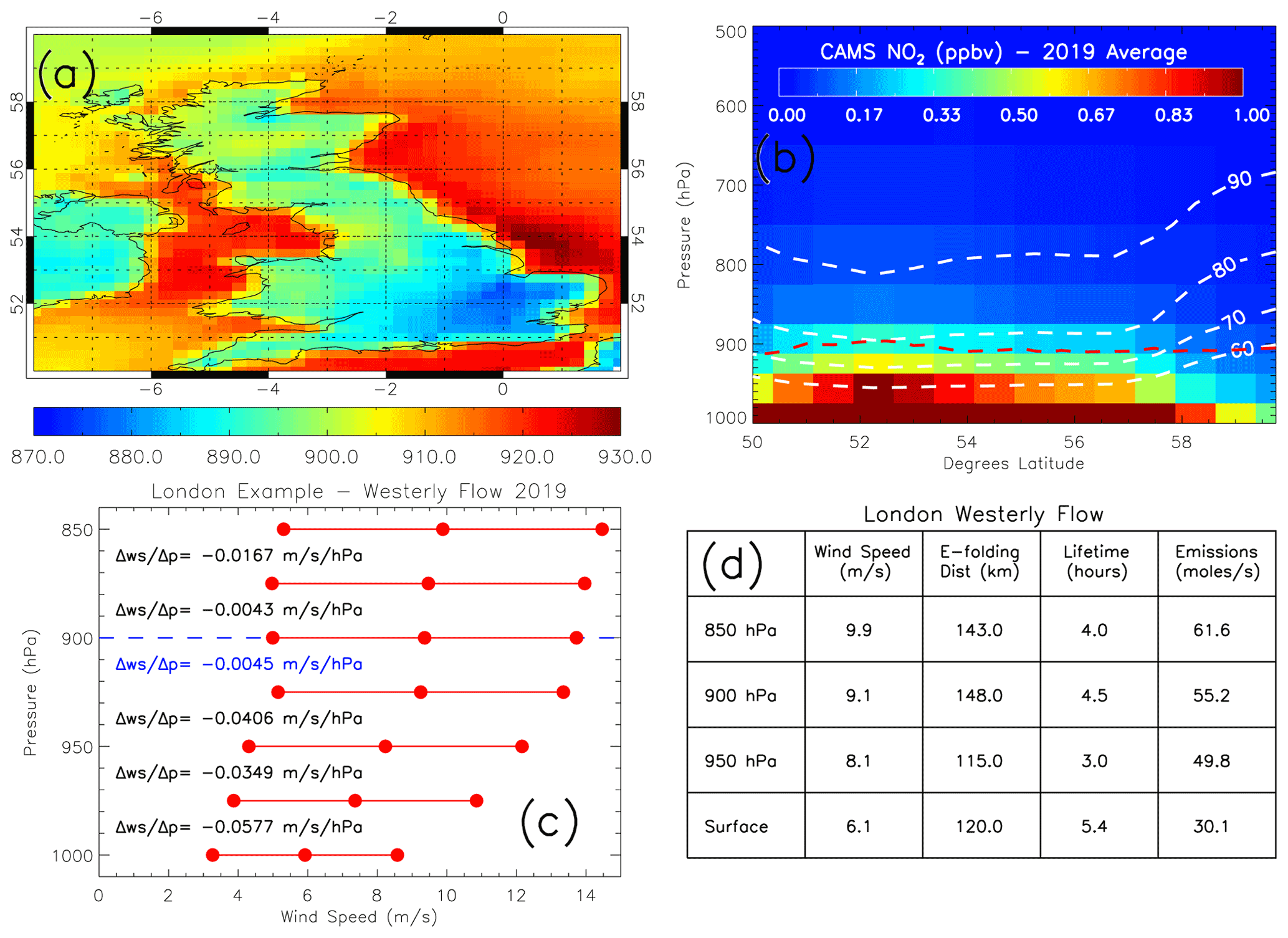
Figure 1 (a) ERA-5 UK boundary layer pressure (hPa) sampled at 13:00 LT (to coincide with the TROPOMI overpass time) and averaged for 2019. (b) CAMS reanalysis zonal (8.0^∘ W–2.0^∘ E) average latitude–pressure NO₂ (ppbv) cross section over the UK between the surface and 500 hPa. White dashed lines represent the percentage of the surface-500 hPa NO₂ loading between the surface and the respective pressure levels. The red dashed line represents the zonal average boundary layer pressure (hPa). (c) Average (surface to pressure level) wind speed (m s⁻¹), ± the standard deviation, profile over London under westerly flow (determined from the ERA-5 u-wind and v-wind components at each pressure level). $\mathrm{\Delta }ws/\mathrm{\Delta }p$ is the wind speed gradient between pressure levels. The blue text indicates the first small step change in the gradient indicative of reduced flow turbulence and a suitable surface-altitude range to average the winds speeds over. (d) The table shows the impact on the NO_x emission parameters when using different altitudes over which to average the wind speeds.

The NO₂ LD is the product of the source width, which is perpendicular to the wind flow, and the source-width-average TCNO₂ (i.e. for each downwind grid box from the source, the corresponding perpendicular rows between the source edges are averaged together) profile downwind from the source on a grid box by grid box basis as shown in Eq. (2).

$$\begin{array}{}\text{(2)}& {\mathrm{NO}}_{\mathrm{2}}{\mathrm{LD}}_{i=\mathrm{1},N}={\displaystyle \frac{{\sum }_{j=\mathrm{1}}^n{\mathrm{TCNO}}_{\mathrm{2}i,j}}{n}}\times w,\end{array}$$

where NO₂ LD (mol m⁻¹) is the NO₂ line density, i is the grid box index downwind of the source starting at i=1 going to i=N at background point B, TCNO₂ is the tropospheric column NO₂ grid box value (mol m⁻²) at point i and j is the grid box index for the number of grid boxes n, perpendicular to the downwind profile, which fit across the width of the source at grid box i downwind, and w is the source width (m) (i.e. source width perpendicular to the downwind profile) of the NO₂ source. Though the source width and length are subjective choices between the source edge locations, the same source width and length values are used when deriving the TROPOMI NO_x emissions and summing up the NAEI NO_x emissions over the source region. As the source emissions will be a function of the source width (i.e. larger at the source centre and lower at the source edge), the mean TCNO₂ downwind profile (i.e. rows averaged across the source width) is representative of the source-average NO₂ emission.

Figure 2a shows the difference between TROPOMI TCNO₂ sampled under westerly flow and the long-term average based on London u- and v-wind components, where there are clear downwind positive anomalies $>\mathrm{3.0}\times {\mathrm{10}}^{-\mathrm{5}}$ mol m⁻². Similarly, in Fig. 2b, the downwind plume (e.g. westerly flow over London) has typically larger NO₂ LD values than the all-flow (i.e. all wind directions) NO₂ LD. The full NO₂ mass emitted from the source in the NO₂ LD is the summation of the wind-flow NO₂ LD from the source up to point B minus the background value from all downwind pixels over this profile segment. A reasonable estimate of when the wind-flow NO₂ LD reaches B, for more isolated NO₂ sources, is when it intersects with the all-flow NO₂ LD profile (i.e. returns to normal levels). However, when there are substantial upwind NO₂ sources, this can yield wind-flow NO₂ LD profiles which never intersect with the all-flow NO₂ LD profile within the domain (e.g. see the Birmingham example in Fig. 3a and b). Therefore, to determine when B, in the downwind direction, has been reached, a running t-test was applied to the wind-flow NO₂ LD profile to determine where turning points or levelling off occurred. Such a substantial change in the NO₂ LD profile gradient is indicative of the background level being reached and/or potentially another source being identified (e.g. in Fig. 2b there is evidence of other NO₂ sources downwind of London several hundred kilometres away over continental Europe). As such a test can be sensitive to noise in the TCNO₂ data, a 10-pixel (0.5^∘) running average wind-flow NO₂ LD profile was calculated. This smoothed out the noise from the downwind profile and allowed for the detection of larger-scale NO₂ LD changes. The running t-test was applied to this using two windows (i.e. a moving centre point with a window each side of 0.5^∘) and the t-test significance between the two window averages determined. This yielded a t-test significance/p-value distance series from the source. When a substantial change in the NO₂ LD gradient occurred, the t-test p-values would increase, peak and then drop off. This change in the gradient of the t-test p-values identified the location of any NO₂ LD step changes in the profile. The green line in Fig. 2b shows where the t-test p-values peaked and that there are turning points in the wind-flow NO₂ LD profile. Such a reduction in the wind-flow NO₂ LD profile gradient is suggestive of the plume reaching B as NO₂ levels have stabilised. However, in Fig. 2b, there are multiple locations potentially meeting these criteria. In reality, the turning points further downwind of London are sources from the Benelux region. The red dot represents the first instance, after the initial near-source wind-flow NO₂ LD peak, where the gradient in the running t-test p-value profile changes sign (i.e. positive to negative or vice versa).

Figure 2 (a) TROPOMI TCNO₂ (10⁻⁵ mol m⁻²) sub-sampled under westerly flow (defined over London, black dot) minus the long-term average (February 2018 to January 2020). The dashed box represents the width of the source and distance between the source and background. (b) Downwind NO₂ LD from London (black: westerly flow, blue: all-flow average) with the corresponding running t-test p-value (green line). The red dot represents the location of the background level determined by the turning point in the running t-test p-value time series. (c) The westerly flow and all-flow NO₂ LD between the peak westerly flow NO₂ LD value and the background value. The red line represents the e-folding distance fit with the corresponding R² and root mean square error (RMSE) between the westerly flow NO₂ LD and fit profile. N represents the number of days classified under westerly flow over London.

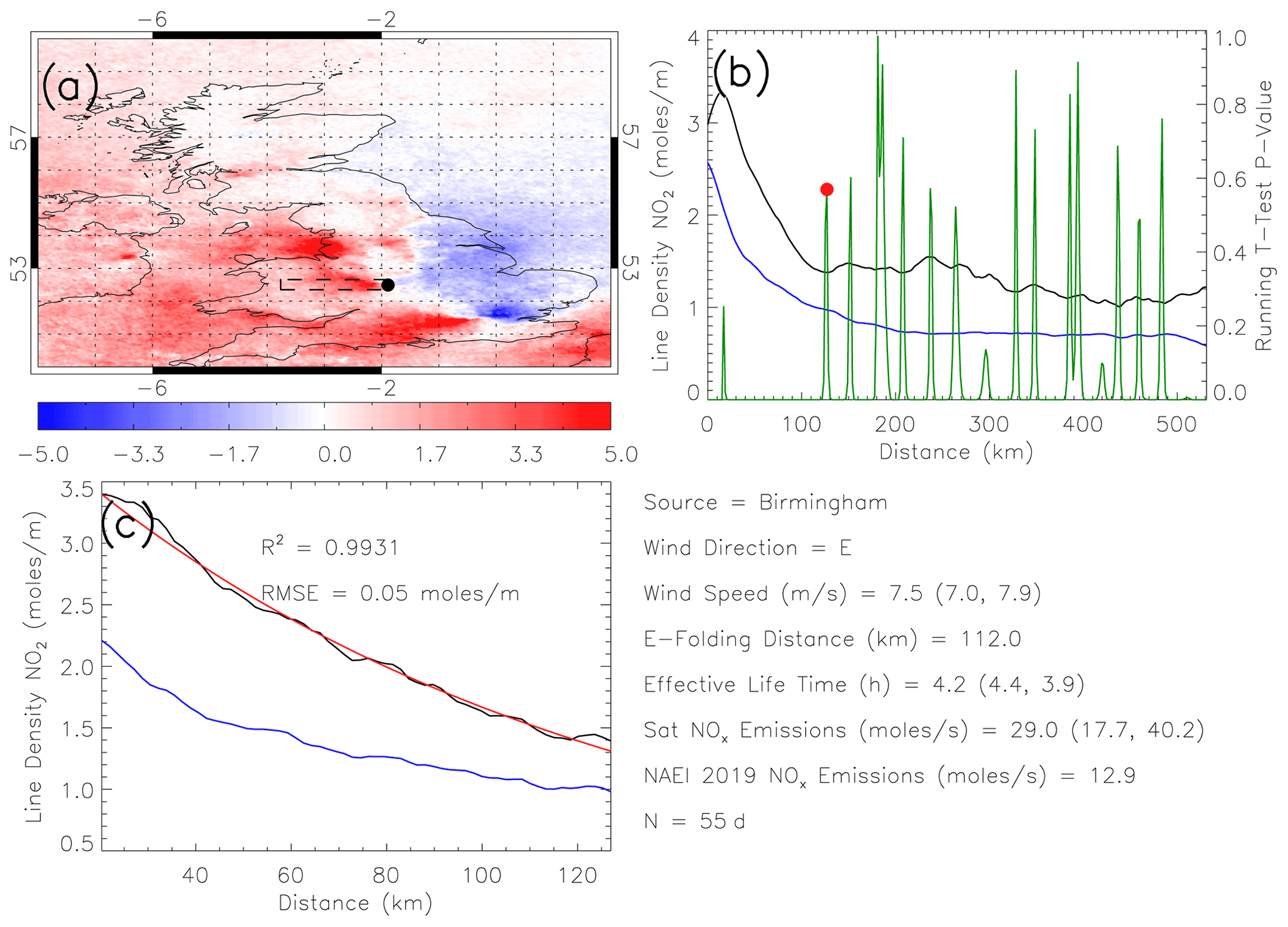
Figure 3 (a) TROPOMI TCNO₂ (10⁻⁵ mol m⁻²) sub-sampled under easterly flow (defined over Birmingham, black dot) minus the long-term average (February 2018 to January 2020). The dashed box represents the width of the source and distance between the source and background. (b) Downwind NO₂ LD from Birmingham (black: easterly flow, blue: all-flow average) with the corresponding running t-test p-value (green line). The red dot represents the location of the background level determined by the turning point in the running t-test p-value time series. (c) The easterly flow and all-flow NO₂ LD between the peak easterly flow NO₂ LD value and the background value. The red line represents the e-folding distance fit with the corresponding R² and RMSE between the easterly flow NO₂ LD and fit profile. N represents the number of days classified under easterly flow over Birmingham.

The loss term $e^{\frac{-t}{\mathit{\tau }}}$ is dependent upon τ and is determined by applying an e-folding distance fit between the near-source peak wind-flow NO₂ LD value and B (i.e. we assume this function is valid only between these two points) before dividing by ws to get τ. Here, a range of e-folding distances are tested in the loss term $e^{\frac{-t}{\mathit{\tau }}}$ to find the distance value which yields the lowest root mean square error (RMSE) and a large R² (Pearson correlation coefficient squared) value between the e-folding distance fit (red line, Fig. 2c) and the wind-flow NO₂ LD (black line, Fig. 2c). In the case of London, this yielded an e-folding distance of 148.0 km and τ of 4.5 h (4.7 and 4.3 h) based on the average ws=9.1 m s⁻¹ with an uncertainty range (±0.4 m s⁻¹; i.e. ±1-sigma standard error) of 8.7 to 9.5 m s⁻¹ (i.e. a slower/faster wind speed yields a longer/shorter lifetime). The effective lifetime derived here for London and other UK cities is typically consistent with values from other studies (e.g. Beirle et al., 2011, and Verstraeten et al., 2018) for European cities (i.e. 1.0–10.0 h).

The top-down E is calculated from Eq. (1), and this emissions flux of NO₂ (mol s⁻¹) is converted to emissions of NO_x (mol s⁻¹) using the factor f for comparison with the bottom-up inventories. This is done by scaling the NO₂ emissions by 1.32 based on the NO:NO₂ concentration ratio (0.32) in urban environments at midday (Seinfeld and Pandis, 2006; Liu et al., 2016). Verstraeten et al. (2018) used modelled NO and NO₂ concentrations to derive a scaling more representative of the chemistry of the source. They estimate there is a 10 % uncertainty (similar to Beirle et al., 2011), but as the modelled NO₂:NO_x ratio is based on the input emissions, for which the satellite data are being used to evaluate, this process is rather circular and not independent.

Here, the top-down NO_x emissions are derived by sampling TCNO₂ data under different wind directions in all seasons. Several studies, such as Beirle et al. (2011), have gone a step further and used TCNO₂ data to derive seasonal emissions. Unfortunately, here we are restricted to looking at annually derived emissions due to (1) the TROPOMI TCNO₂ record only starting in February 2018, (2) the COVID-19 pandemic resulting in a dramatic reduction in UK (and global) NO_x emissions (Potts et al., 2021), meaning TCNO₂ data beyond February 2020 could not be used to derive top-down emissions under normal conditions, and (3) the UK being subject to frequently cloudy conditions yielding a reduction in the number of observations from TROPOMI. The latter point predominantly influences TROPOMI retrievals in the winter-time. Therefore, even though we sample TCNO₂ data in all seasons, there is likely to be a tendency towards summer-time TCNO₂ values, when TCNO₂ values tend to be lower (e.g. Pope et al., 2015), potentially leading to a low bias in the derived top-down NO_x emissions.

To investigate the total errors in the derived NO_x emissions from TROPOMI, we have included errors from all the input terms. These include the enhancement in the TNCO₂ data, the e-folding distance x_o, the wind speed ws, the source width w, the NO₂-to-NO_x conversion factor f and the distance d between the source and B. When combined, this yields the total error in Eq. (3).

$$\begin{array}{}\text{(3)}& \begin{array}{rl}& \mathrm{\Delta }E=\\ & E\sqrt{{\displaystyle \frac{\mathrm{\Delta }{\mathit{\varphi }}^{\mathrm{2}}}{{\mathit{\varphi }}^{\mathrm{2}}}}+{\displaystyle \frac{\mathrm{\Delta }w{s}^{\mathrm{2}}}{w{s}^{\mathrm{2}}}}+{\displaystyle \frac{\mathrm{\Delta }{w}^{\mathrm{2}}}{w^{\mathrm{2}}}}+{\displaystyle \frac{\mathrm{\Delta }{f}^{\mathrm{2}}}{f^{\mathrm{2}}}}+{\displaystyle \frac{d^{\mathrm{2}}}{x_o^{\mathrm{2}}}}\left[{\displaystyle \frac{\mathrm{\Delta }{d}^{\mathrm{2}}}{d^{\mathrm{2}}}}+{\displaystyle \frac{\mathrm{\Delta }{x}_o^{\mathrm{2}}}{x_o^{\mathrm{2}}}}\right]}\end{array}\end{array}$$

In the total error expression, we have set $\mathit{\varphi }=\stackrel{\mathrm{‾}}{{\mathrm{NO}}_{\mathrm{2}}}-B$, where $\stackrel{\mathrm{‾}}{{\mathrm{NO}}_{\mathrm{2}}}$ is the average TCNO₂ value (mol m⁻²) for all grid cells between the source and B (i.e. background TCNO₂ value) in the downwind profile. Here, we take $\mathit{\varphi }\times d\times w$ to be a suitable estimate of the full NO₂ emission loading from the source (i.e. the numerator of Eq. 1). Regarding the errors (i.e. terms with Δ in front), based on Beirle et al. (2011), we assign errors of 10 % to f and w. As x_o and d are distance metrics as well, with no clear way to quantify the errors in these terms, we have assigned them with 10 % errors also. The ws error is based on the standard error in the sample (i.e. the number of days selected for each flow regime). For the enhancement in TCNO₂ from the source (i.e. ϕ), we have conservatively taken the largest precision error value from all TCNO₂ values between the source and B, which forms $\stackrel{\mathrm{‾}}{{\mathrm{NO}}_{\mathrm{2}}}$.

3 Results

3.1 NO_x sources

Surface emissions and observed TCNO₂ represent different quantities and are influenced by different processes. However, the short NO₂ lifetime of a few hours (Schaub et al., 2007; Pope et al., 2015) means there is a sharp gradient between sources and the background levels. Therefore, we can use the satellite TCNO₂ observations to provide some constraint on the spatial distribution of the NO_x emissions. In Fig. 4, spatial maps over south-eastern (Fig. 4a and c) and northern England (Fig. 4b and d) show evidence of co-located TCNO₂ and NO_x emission hotspots, especially over many of the UK cities shown by circles. Here, both data sets have been mapped onto the spatial resolution of $\mathrm{0.025}{}^{\circ }\times \mathrm{0.025}{}^{\circ }$. In south-eastern England, TCNO₂ and NO_x emissions peak over London at over $\mathrm{14.0}\times {\mathrm{10}}^{-\mathrm{5}}$ mol m⁻² and approximately >2.0 µg m⁻² s⁻¹, respectively. A secondary peak is also observed over western London for both quantities at similar levels. There are further co-located hotspots over Southampton (TCNO₂ ∼ 8.0–$\mathrm{9.0}\times {\mathrm{10}}^{-\mathrm{5}}$ mol m⁻², NO_x > 2.0 µg m⁻² s⁻¹), Portsmouth (TCNO₂ ∼ 6.0–7.0 × 10⁻⁵ mol m⁻², NO_x ∼ 1.0–1.5 µg m⁻² s⁻¹), Brighton (TCNO₂ ∼ 5.0–$\mathrm{6.0}\times {\mathrm{10}}^{-\mathrm{5}}$ mol m⁻², NO_x∼0.5–0.8 µg m⁻² s⁻¹), Oxford (TCNO₂∼7.0–$\mathrm{7.5}\times {\mathrm{10}}^{-\mathrm{5}}$ mol m⁻², NO_x∼0.7–1.0 µg m⁻² s⁻¹) and Chelmsford (TCNO₂∼8.5–$\mathrm{9.5}\times {\mathrm{10}}^{-\mathrm{5}}$ mol m⁻², NO_x∼0.5 µg m⁻² s⁻¹). In northern England and the Midlands, peak TCNO₂ and NO_x emissions are located over Manchester (TCNO₂∼10.0–$\mathrm{11.0}\times {\mathrm{10}}^{-\mathrm{5}}$ mol m⁻², NO_x∼1.0–1.5 µg m⁻² s⁻¹), Birmingham (TCNO₂∼8.0–$\mathrm{9.0}\times {\mathrm{10}}^{-\mathrm{5}}$ mol m⁻², NO_x∼1.0–1.5 µg m⁻² s⁻¹), Leeds (TCNO₂∼8.0–$\mathrm{9.0}\times {\mathrm{10}}^{-\mathrm{5}}$ mol m⁻², NO_x∼1.0–1.5 µg m⁻² s⁻¹) and Liverpool (TCNO₂∼7.0–$\mathrm{8.0}\times {\mathrm{10}}^{-\mathrm{5}}$ mol m⁻², NO_x∼0.5–1.0 µg m⁻² s⁻¹).

Figure 4 TROPOMI TCNO₂ ($\times {\mathrm{10}}^{-\mathrm{5}}$ mol m⁻²) average for February 2018 to January 2020 across (a) south-eastern and (b) northern England. Black circles represent city locations. NAEI NO_x emissions (µg m⁻² s⁻¹) for 2019 across (c) south-eastern and (d) northern England. Red circles represent city locations. Panels (e)–(h) represent the correlation of normalised TCNO₂ and NO_x emissions for UK cities. The green dashed line is the 1:1 line. Each source is normalised by the average of all the sources. The four panels also represent city means using varying pixel ranges around the source (i.e. 1×1, 3×3, 5×5 and 7×7 grid pixels). The correlations between the city-scale normalised NO_x emissions and TCNO₂ are shown (R).

To quantify the spatial relationship between the TCNO₂ and NO_x emissions over source regions, the corresponding pixels of both data sets were sub-sampled for each UK city (79 in total), normalised by the sample mean and correlated against each other (red circles, Fig. 4e), which yielded a correlation $R_{\mathrm{city}\mathrm{1}\times \mathrm{1}}=\mathrm{0.35}$ (i.e. city1×1 represents 1 grid box ×1 grid box or $\mathrm{0.025}{}^{\circ }\times \mathrm{0.025}{}^{\circ }$ around where the city centre is located). However, as atmospheric NO₂ is subject to chemical reactions and meteorological processes (e.g. transport), the signal around source regions is more diluted and the peak TCNO₂ not necessarily centred on the source. To allow for that, the spatial resolution of the quantities over each source was degraded, averaging over 3×3 (Fig. 4f), 5×5 (Fig. 4g) and 7×7 (Fig. 4h) grid cells, and the correlation recalculated (e.g. city3×3 represents 3 grid boxes ×3 grid boxes or $\mathrm{0.075}{}^{\circ }\times \mathrm{0.075}{}^{\circ }$ around where the city centre is located). This resulted in correlations of $R_{\mathrm{city}\mathrm{3}\times \mathrm{3}}=\mathrm{0.53}$, $R_{\mathrm{city}\mathrm{5}\times \mathrm{5}}=\mathrm{0.62}$ and $R_{\mathrm{city}\mathrm{7}\times \mathrm{7}}=\mathrm{0.52}$. The correlation for the full domain (i.e. the UK) was R_all=0.20. As expected, the correlation for all grid pixels (e.g. including pixels over the sea) is weak, where long-range transport of NO₂ can yield spatial variability in background regions with corresponding zero emission pixels. The R_city1×1, R_city3×3, R_city5×5 and R_city7×7 correlations were all larger. The largest city-scale correlation was for the R_city5×5 values, where the spatial variability has been smoothed and is representative of the more diffuse pattern of TCNO₂. However, the R_city7×7 ($\mathrm{0.175}{}^{\circ }\times \mathrm{0.175}{}^{\circ }$ or ∼15–20 km ×15–20 km) correlation is lower than the R_city5×5 value, suggesting that this scale is larger than most UK city sizes. Overall, for all R values, except for R_all, there are statistically significant positive correlations at the 90 % confidence level (CL) or above (>95 % CL for R_city3×3, R_city5×5 and R_city7×7). Therefore, the city-scale emission-satellite correlations provide confidence in the spatial distribution of the NAEI NO_x emissions based on the observed satellite TCNO₂.

3.2 Satellite NO₂ and emission NO_x trends

To evaluate the temporal evolution of the NAEI emissions, we use the long-term satellite record of TCNO₂ from OMI between 2005 and 2015. Annual total UK emissions of NO_x (expressed as NO₂ here) from the NAEI start in 1970 and continue to the present day (typically with a lag of approximately 2 years). Annual spatial maps of the NAEI also exist over the same time period. However, while there is a consistent methodology for the UK total estimates, the mapping methodology updates between years (NAEI, 2017). Therefore, instead of performing trends on the maps, we focus on trends in the UK NO_x emission totals. For OMI, we have taken a similar broad-scale approach focussing on averaged TCNO₂ across England (defined as 3^∘ W–2^∘ E, 50–54^∘ N). We focus on England as the majority of large UK sources with reasonable spatiotemporal coverage are located here and have clearly defined trends over source regions. Pope et al. (2018) showed significantly (at the 95 % CL) decreasing trends over London, Birmingham, Manchester and the Yorkshire power stations of between 1.5 % and 2.3 % per year. OMI measurements can be subject to large uncertainties and variability, so this analysis also investigates trends in a range of OMI TCNO₂ percentiles over time. To estimate the annual absolute England total NAEI NO_x emissions, we summed the emissions data for England (same geographical definition as for OMI above) from the 2019 NAEI NO_x emissions map and imposed the UK total NO_x trend on it. Here, we use a simple linear fit which yields an annual decrease in the UK total NO_x emission of 4.4 %. The relative rate of change is the same for the England total NO_x emissions, but the absolute values are lower than the UK total NO_x emissions (Fig. 5a).

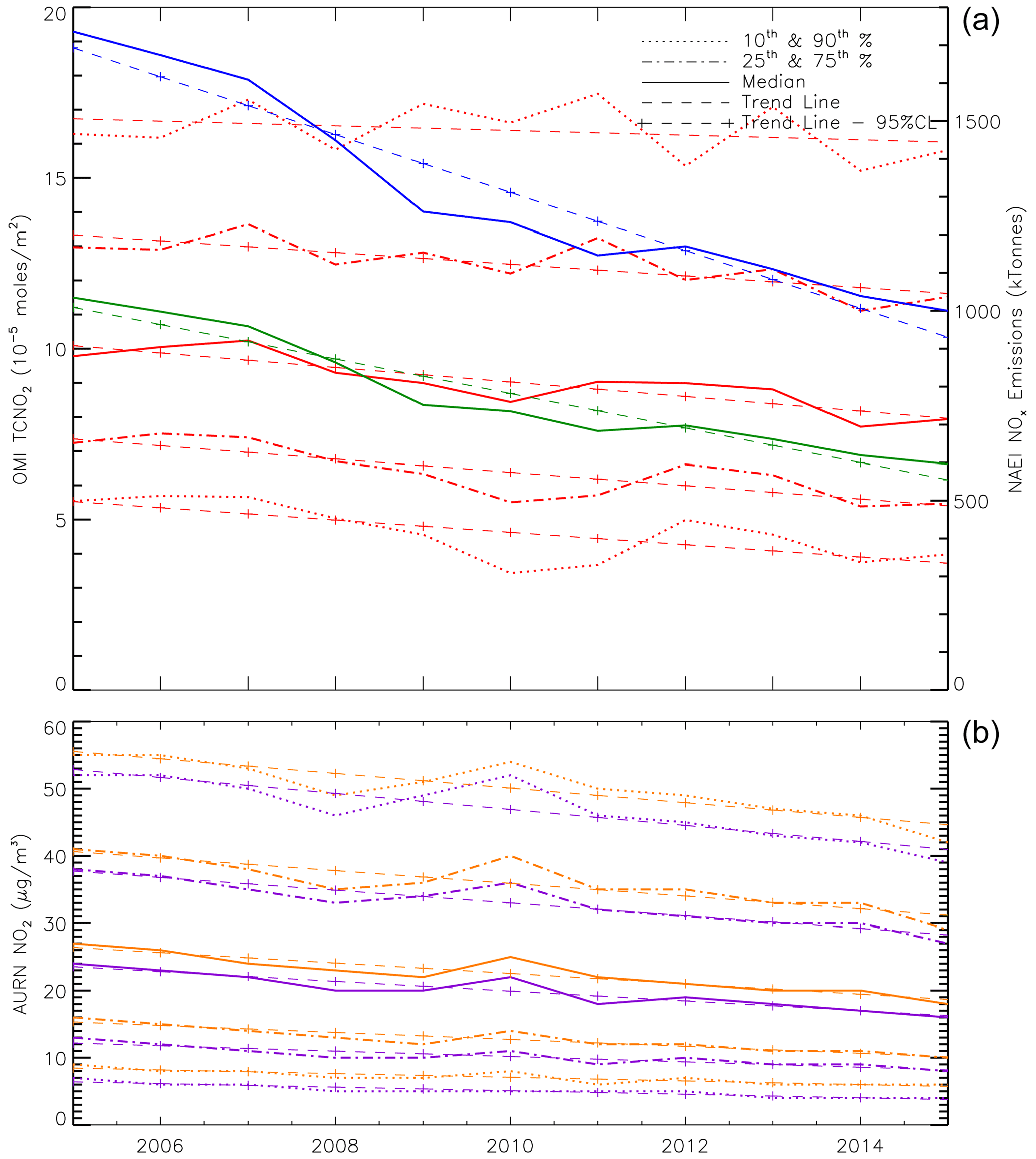
Figure 5 Panel (a) shows time series (2005 to 2015) in OMI TCNO₂ ($\times {\mathrm{10}}^{-\mathrm{5}}$ mol m⁻²) and NAEI NO_x emission totals (kt or Gg). OMI median, 10th and 90th and 25th and 75th percentiles are represented by solid, dotted and dot-dashed lines, respectively. NAEI NO_x emission totals for the UK and England are represented by the blue and green solid lines. Here, the OMI TCNO₂ has been averaged over England (defined as 3^∘ W–2^∘ E, 50–54^∘ N), and while the UK NO_x emission totals are directly reported by the NAEI, the England NO_x emission totals have been summed over the emissions maps for the same England definition used for OMI (see Sect. 3.2 for more information). In panel (b), AURN surface NO₂ (µg m⁻³) times series are shown for the UK (purple) and England (orange). Trend lines are shown by dashed and dash-crossed lines for insignificant and significant trends (at the 95 % confidence level).

Over the 2005–2015 period, the England average OMI TCNO₂ trends in the 10th, 25th, 50th, 75th and 90th percentiles are $-\mathrm{0.18}\times {\mathrm{10}}^{-\mathrm{5}}$ mol m⁻² yr⁻¹ (−3.2 % yr⁻¹), −0.20 × 10⁻⁵ mol m⁻² yr⁻¹ (−2.7 % yr⁻¹), −0.21 × 10⁻⁵ mol m⁻² yr⁻¹ (−2.2 % yr⁻¹), −0.17 $\times {\mathrm{10}}^{-\mathrm{5}}$ mol m⁻² yr⁻¹ (−1.3 % yr⁻¹) and −0.07 × 10⁻⁵ mol m⁻² yr⁻¹ (−0.4 % yr⁻¹), respectively (Fig. 5). All of the satellite trends are significant at the 95 % CL, except for the 90th percentile. The UK and England total NO_x emission trends between 2005 and 2015 are −76.3 and −45.5 kt yr⁻¹ (both −4.4 % yr⁻¹). The OMI TCNO₂ trends range between −3.2 % and −0.4 % depending on the data percentile used to generate the average England TCNO₂ annual time series. We also calculated annual trends in UK and England (same definition as above) surface NO₂ observations (Fig. 5b) from the Automated Urban and Rural Network (AURN) (AURN, 2021a). Here, we used urban background, suburban and rural sites. For the 10th, 25th, 50th, 75th and 90th percentiles, UK (England) trends are −0.26 (−0.27) µg m⁻³ yr⁻¹, −0.40 (−0.52) µg m⁻³ yr⁻¹, −0.73 (−0.77) µg m⁻³ yr⁻¹, −0.95 (−0.95) µg m⁻³ yr⁻¹ and −1.19 (−1.09) µg m⁻³ yr⁻¹. This corresponds to −3.77 % yr⁻¹ (−3.03 % yr⁻¹), −3.07 % yr⁻¹ (−3.24 % yr⁻¹), −3.03 % yr⁻¹ (−2.86 % yr⁻¹), −2.49 % yr⁻¹ (−2.31 % yr⁻¹) and −2.29 % yr⁻¹ (−1.98 % yr⁻¹). Therefore, the NAEI NO_x emissions trend is of similar magnitude and direction to that of the observations. The differences are most likely explained by the non-linear conversion of emissions to atmospheric concentrations (i.e. complex meteorology and chemistry). The likely drivers for decreases in UK NO_x emissions and NO₂ concentrations include a shift to cleaner energy sources (e.g. National Emissions Ceilings Regulations 2018; DEFRA, 2018b), regulations on industrial and power generation emissions (Environmental Permitting Regulations 2016; UK Government, 2016) and tighter emissions for vehicles (e.g. Euro 6 emissions standards). Overall, these results provide confidence in the use of the satellite data as a tool to evaluate bottom-up emission trends.

3.3 Top-down NO_x emissions

The top-down NO_x emission rate for London under westerly flow (Fig. 2) is 55.2 mol s⁻¹ (37.7, 72.7 mol s⁻¹, i.e. satellite total error range), while the NAEI flux is 30.9 mol s⁻¹. Here, the NAEI has a low bias with the top-down estimate and sits outside the uncertainty range. The top-down emissions are based on 2 years, so the flux should be representative of an annual emission rate, corresponding to the NAEI reporting. In the case of Birmingham (Fig. 3a), under easterly flow, there is a visible plume (i.e. positive differences of 2.0–$\mathrm{3.0}\times {\mathrm{10}}^{-\mathrm{5}}$ mol m⁻²) superimposed on a background enhancement (0.5–$\mathrm{1.0}\times {\mathrm{10}}^{-\mathrm{5}}$ mol m⁻²). As a result, the wind-flow NO₂ LD is always larger than the all-flow NO₂ LD and never reaches the background level (i.e. zero differences in Fig. 3a) within the domain for which the TROPOMI TCNO₂ data have been processed (e.g. there are positive differences in between the source, Birmingham, and the west of the domain, 8^∘ W). Therefore, the running t-test methodology is used to determine when the wind-flow NO₂ LD reaches a steady background state B, as shown in Fig. 3b. Overall, the NAEI (12.9 mol s⁻¹) underestimates the top-down emissions for Birmingham under easterly flow (29.0 (17.7, 40.2) mol s⁻¹).

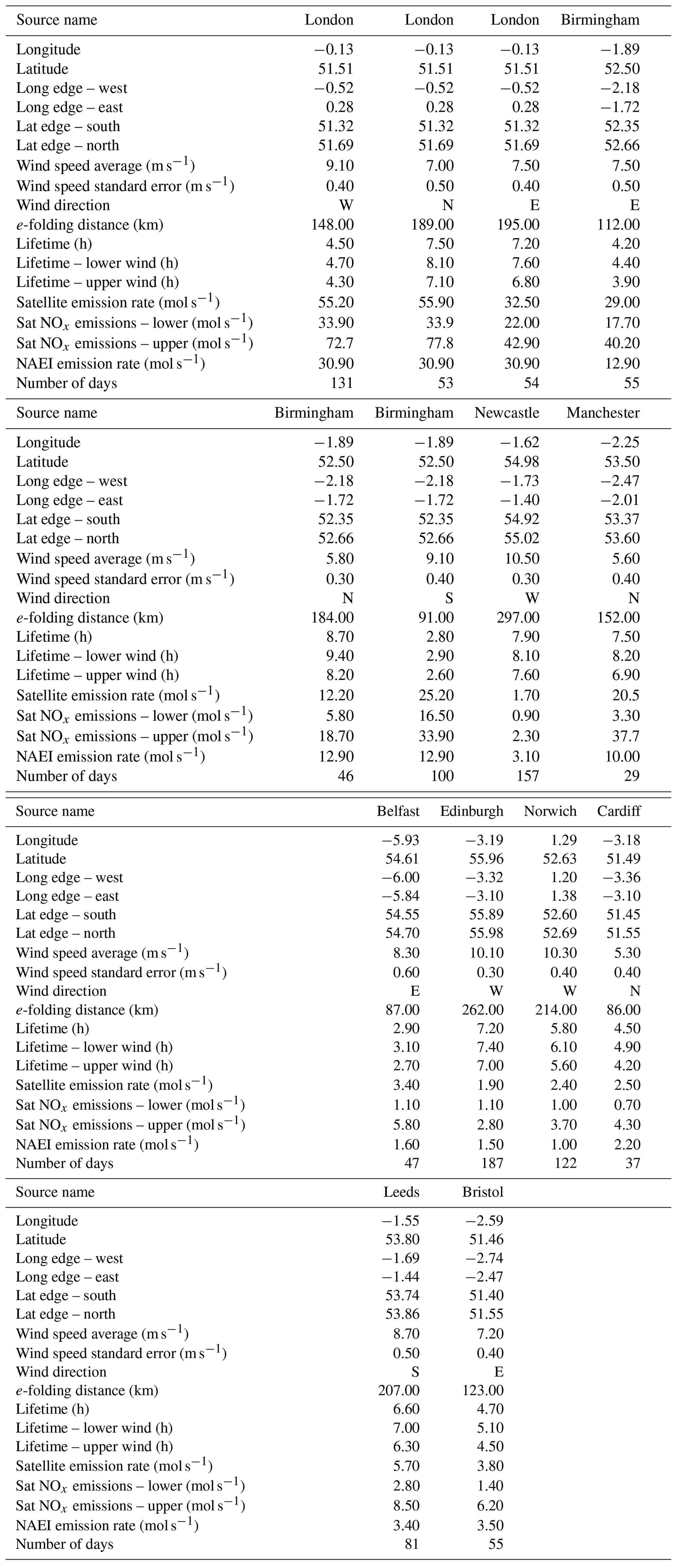
Our methodology was applied to 10 city sources where sources had suitable downwind TCNO₂ enhancements to derive NO₂ LDs and top-down emissions (Fig. 6). A suitable downwind TCNO₂ enhancement was subjectively identified when a clear TCNO₂ enhancement (i.e. positive anomalies) under a specific wind flow/direction occurred and a realistic lifetime (i.e. in the range of the literature – e.g. Verstraeten et al., 2018) could be derived from the downwind TCNO₂ profile of the target source. These are shown in Table 1. Where top-down emissions could be derived for sources over several wind directions, they were averaged together. The TCNO₂ response to mesoscale and synoptic weather systems (i.e. large-scale flow) can be seasonally influenced (e.g. Pope et al., 2015), with some wind directions occurring more frequently in certain seasons. Therefore, top-down NO_x emission estimates derived from several wind directions for a particular source, though sampled throughout all months, can vary depending on the seasonal influence on the observed TCNO₂ for which the wind direction more frequently occurs. The top-down emissions derived here suggest that the NAEI bottom-up emissions for the largest sources such as London and Birmingham are underestimated. The top-down emissions for London and Birmingham are 47.9 (31.2, 64.5) mol s⁻¹ and 22.1 (13.3, 30.9) mol s⁻¹, with corresponding NAEI emissions of 30.9 mol and 12.9 mol s⁻¹, respectively. The NAEI (10.0 mol s⁻¹) also underestimates the emissions for Manchester 20.5 (3.3, 37.7) mol s⁻¹, but the top-down emission uncertainty is large (dominated by the smaller sample size of 29 d and large precision errors in the TCNO₂ data) and so sits within its uncertainty range.

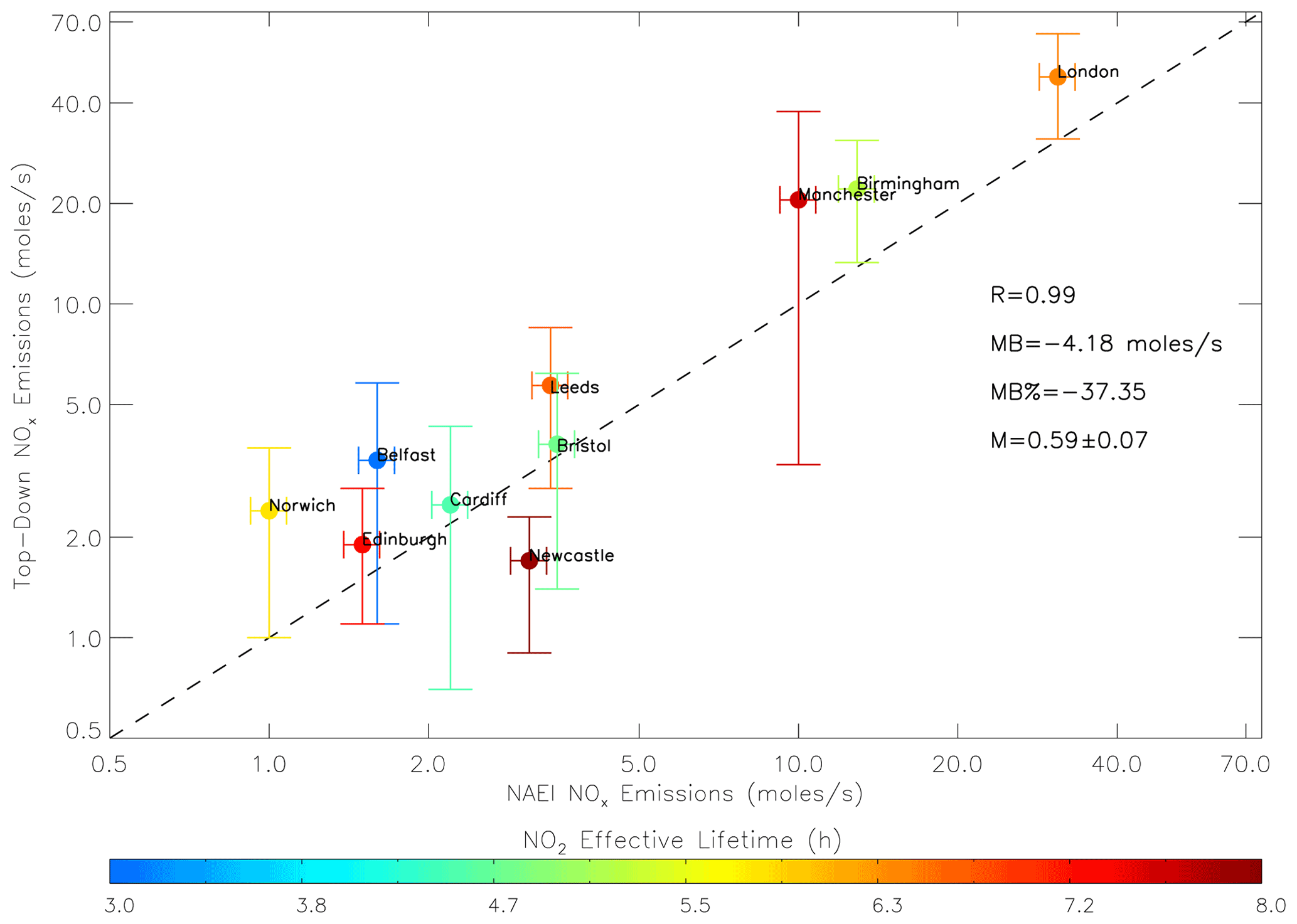
Figure 6 NAEI and top-down (TROPOMI) NO_x emissions (mol s⁻¹) for 10 UK cities coloured by the NO₂ effective lifetime (h). Where there is more than one top-down estimate for a city from multiple wind directions, the corresponding emission rates and lifetimes have been averaged together. The correlation (R), mean bias (MB, mol s⁻¹, i.e. NAEI-top down), percentage mean bias (MB%) and linear fit (M, i.e. top-down vs. NAEI) are also shown. NAEI uncertainty is ±7.8 % (DEFRA, 2018b), and the top-down uncertainty range is based on the satellite errors. The black dashed line represents the 1:1 relationship, and both axes are on log scales.

For the smaller sources (e.g. Edinburgh, Bristol, Cardiff, Leeds, Norwich and Belfast), the comparisons are in better agreement with the NAEI and are located within the top-down emissions uncertainty ranges. However, for Newcastle the NAEI emissions (3.1 mol s⁻¹) are substantially larger than the top-down estimate (1.7 (0.9, 2.3) mol s⁻¹). For the NO₂ effective lifetime, we find it ranges between 2.9 and 7.9 h, which is consistent with values in the literature (e.g. Schaub et al., 2007; Pope et al., 2015). For all cities in Fig. 6 there is a strong correlation (0.99) between the NAEI and top-down emission sources investigated here, but the NAEI has a low bias of −4.18 mol s⁻¹ (−37.4 %) on average, dominated by the larger sources (i.e. London and Birmingham). These metrics were calculated in linear space.

4 Conclusions

We have evaluated relationships between satellite observations (TROPOspheric Monitoring Instrument, TROPOMI) of tropospheric column nitrogen dioxide (TCNO₂) and the UK National Atmospheric Emissions Inventory (NAEI) for nitrogen oxides (NO${}_x=\mathrm{NO}+{\mathrm{NO}}_{\mathrm{2}}$). Although they are different quantities, the short NO₂ lifetime means that our comparison can serve as a useful and important tool to evaluate bottom-up emissions. Here, spatial comparison of the TROPOMI TCNO₂ with the NAEI highlights consistency over the source regions, with co-located peak values in the respective data sets. Correlation analysis of TCNO₂ and NO_x emissions over the UK cities indicates moderate spatial agreement, with R ranging between 0.4 and 0.6 (significant at the >90 % confidence level). Analysis of long-term satellite records of TCNO₂ (from the Ozone Monitoring Instrument (OMI), 2005–2015) show comparable negative trends with the NAEI NO_x emissions with rates of −2.2 % yr⁻¹ and −4.4 % yr⁻¹, respectively. Though the relative NAEI trend is larger than OMI, meteorological conditions and photochemistry will control the atmospheric response to a change in NO_x emissions, as seen by OMI. It is also possible that the NAEI overestimates the decreasing NO_x emissions trend.

We have also used TROPOMI data to derive top-down city-scale estimates of UK NO_x emissions. While it can still be challenging to derive emissions from city-scale sources (e.g. frequent cloud cover in the UK), we estimate top-down emissions fluxes (using satellite data between February 2018 and January 2020) for several cities. Most of the city sources show reasonable agreement, but for larger sources like London and Birmingham, the top-down emission values are substantially larger than those in the NAEI for 2019. Overall, as far as we are aware, this study represents the first robust attempt to use satellite observations of TCNO₂ to evaluate and constrain the official UK bottom-up NAEI. We find spatial and temporal agreement between the two quantities but find evidence that the NAEI NO_x emissions for larger sources (e.g. London) may be too low (i.e. by >25 %), sitting outside the top-down emission uncertainty ranges. To fully understand the discrepancies and the drivers of these NO_x emissions differences, further investigation is required.

Table 1 List of top-down NO_x (mol s⁻¹) emission estimates for UK city sources under different wind directions. The Sat NO_x emissions lower and upper ranges represent the emission flux ± the total error.