Quantification and assessment of methane emissions from offshore oil and gas facilities on the Norwegian continental shelf

The oil and gas (O&G) sector is a significant source of methane (CH₄) emissions. Quantifying these emissions remains challenging, with many studies highlighting discrepancies between measurements and inventory-based estimates. In this study, we present CH₄ emission fluxes from 21 offshore O&G facilities collected in 10 O&G fields over two regions of the Norwegian continental shelf in 2019. Emissions of CH₄ derived from measurements during 13 aircraft surveys were found to range from 2.6 to 1200 t yr⁻¹ (with a mean of 211 t yr⁻¹ across all 21 facilities). Comparing this with aggregated operator-reported facility emissions for 2019, we found excellent agreement (within 1σ uncertainty), with mean aircraft-measured fluxes only 16 % lower than those reported by operators. We also compared aircraft-derived fluxes with facility fluxes extracted from a global gridded fossil fuel CH₄ emission inventory compiled for 2016. We found that the measured emissions were 42 % larger than the inventory for the area covered by this study, for the 21 facilities surveyed (in aggregate). We interpret this large discrepancy not to reflect a systematic error in the operator-reported emissions, which agree with measurements, but rather the representativity of the global inventory due to the methodology used to construct it and the fact that the inventory was compiled for 2016 (and thus not representative of emissions in 2019). This highlights the need for timely and up-to-date inventories for use in research and policy. The variable nature of CH₄ emissions from individual facilities requires knowledge of facility operational status during measurements for data to be useful in prioritising targeted emission mitigation solutions. Future surveys of individual facilities would benefit from knowledge of facility operational status over time. Field-specific aggregated emissions (and uncertainty statistics), as presented here for the Norwegian Sea, can be meaningfully estimated from intensive aircraft surveys. However, field-specific estimates cannot be reliably extrapolated to other production fields without their own tailored surveys, which would need to capture a range of facility designs, oil and gas production volumes, and facility ages. For year-on-year comparison to annually updated inventories and regulatory emission reporting, analogous annual surveys would be needed for meaningful top-down validation. In summary, this study demonstrates the importance and accuracy of detailed, facility-level emission accounting and reporting by operators and the use of airborne measurement approaches to validate bottom-up accounting.

1 Introduction

Concentrations of atmospheric methane (CH₄) have been increasing since 1850, with particularly rapid annual growth rates of over 5 ppb yr⁻¹ observed from 2014 to 2017 (Nisbet et al., 2019). With a radiative forcing of approximately 0.5 W m⁻² (Prather et al., 2001) and a global warming potential 84 times that of CO₂ over a 20-year period (Myhre et al., 2013), CH₄ is the second-most important greenhouse gas. CH₄ emission reduction and mitigation strategies could aid the attainment of climate targets set in the United Nations Framework Convention on Climate Change (UNFCCC) Paris Agreement (Nisbet et al., 2020). In order to inform and direct such efforts, an accurate understanding of the nature and magnitude of anthropogenic and natural sources of CH₄ is essential.

Emissions from the oil and gas (O&G) sector are estimated to account for approximately 22 % of global anthropogenic CH₄ emissions (80 Tg yr⁻¹), though this remains highly uncertain, with estimates ranging from 68 to 92 Tg yr⁻¹ (Saunois et al., 2020). This can be partly attributed to the fact that O&G emissions are associated with a wide range of variable and episodic activities such as minor failures in engineering (Zavala-Araiza et al., 2017), flaring (combustion of the gas), controlled cold venting (discharge of unburned gases into the atmosphere) and other fugitive processes. Large but rare unexpected leaks can also result in significant releases to the atmosphere (Ryerson et al., 2012; Conley et al., 2016; Lee et al., 2018).

There have been limited numbers of studies focussed on emissions from offshore O&G production, relative to onshore facilities (EIA, 2016). The current quantification of emissions from offshore facilities therefore often relies on bottom-up approaches that use activity data and emission factors to derive emissions from a subset of sources and extrapolation to estimate the total emission. However, emission factor calculations rely on representative knowledge of all emission sources, with the potential for systematic error. The International Energy Agency (IEA) Methane Tracker bottom-up estimate of the offshore share of global O&G-related CH₄ emissions is 20 % (IEA, 2021). Top-down emission estimates, such as direct measurements of atmospheric mixing ratios downwind of a source or group of sources, can help to improve bottom-up inventory estimates, which in turn can more meaningfully inform emission mitigation and climate policy. However, the relatively small number of studies on offshore emissions means that there has been little independent data to validate reported emissions. The studies that have taken place (for both onshore and offshore facilities) have consistently reported inventory underestimates of CH₄ and non-methane volatile organic compounds (NMVOCs) from O&G extraction (Xiao et al., 2008; Pétron et al., 2012; Gorchov Negron et al., 2020).

Recently, ship-based campaigns have investigated CH₄ emissions from offshore facilities, including the Gulf of Mexico (Yacovitch et al., 2020) and the North Sea (Riddick et al., 2019). Yacovitch et al. (2020) reported CH₄ emission fluxes in the range of 0 to 190 kg h⁻¹ for 103 offshore facilities in the Gulf of Mexico region. Riddick et al. (2019) investigated CH₄ emissions from eight offshore facilities in the UK part of the North Sea and reported leakage of CH₄ gas from all facilities sampled during primary operations, with a higher measured collective emission compared with estimates from the UK National Atmospheric Emissions Inventory (NAEI) (0.19 % and 0.13 %, respectively). Results from the Riddick et al. (2019) study emphasised a need for further research to accurately determine CH₄ leakages from offshore O&G facilities and to include these in emission inventories. As part of the ACCESS (Arctic Climate Change, Economy and Society) campaign, Roiger et al. (2015) also highlighted the impact of offshore O&G facility emissions on local air quality, including nitrogen oxide (NO_x) emissions and tropospheric ozone (O₃) formation. Gorchov Negron et al. (2020) derived facility-level CH₄ emissions from multiple offshore facilities in the Gulf of Mexico using aircraft observations. These were used alongside production data and inventory estimates to compile an aerial-measurement-based CH₄ emission inventory for the Gulf of Mexico. The inventory was separated into three source categories (producing facilities, non-producing facilities and minor sources, and the largest shallow-water facilities), with each category applying a different emission estimation approach. Comparisons with the US Environmental Protection Agency greenhouse gas inventory showed that measured CH₄ emissions were consistent for deep-water but were a factor of 2 higher for shallow-water facilities. Gorchov Negron et al. (2020) attributed this discrepancy to incomplete platform counts and discrepancies in the emission factors used in the inventory. In contrast, Zavala-Araiza et al. (2021) reported airborne measurements of CH₄ emissions from offshore facilities in the Sureste Basin, Mexico, which were found to be an order of magnitude lower than the Mexican greenhouse gas inventory.

As part of the United Nations Climate and Clean Air Coalition (CCAC) objective to quantify global CH₄ emissions from oil and gas facilities, this study quantifies CH₄ emissions from active O&G facilities on the Norwegian continental shelf using a Lagrangian mass balancing approach, as outlined in France et al. (2021). We report measurements of CH₄ mixing ratios and fluxes sampled by two research aircraft downwind of 21 emitting facilities (out of 25 facilities surveyed) during 13 flights in July and August 2019. The FLEXPART (FLEXible PARTicle) dispersion model was used to confirm the facility origin of sampled CH₄ plumes. Comparisons are made with operator-supplied annualised emission and daily activity data from individual facilities in order to identify agreements or discrepancies, as well as to evaluate the efficacy of emission reporting procedures within the areas of the Norwegian continental shelf covered by this study. In particular, comparison with daily reported activity data is key when variable or episodic sources are present. Emission estimates from an annualised global inventory (Scarpelli et al., 2020) are also compared against measured data to provide insight into the relative accuracy of a hierarchy of emission-accounting approaches.

In Sect. 2, we outline the details of the research aircraft, instrumentation and sampling strategies employed to survey emissions from O&G facilities on the Norwegian continental shelf. In Sect. 3, we describe the methods used to derive CH₄ fluxes from individual facilities and the uncertainties implicit to the mass balance method. In Sect. 4, we discuss the calculated facility-level flux results and compare them to estimates from both a global inventory and operator-reported emission and activity data. In Sect. 4, we also discuss the relevance of platform operational data and CH₄ loss rate calculations and provide an outlook for continued research in this field.

2 Methods

In this section, we describe the flight surveys, the two aircraft platforms and instrumentation used to record measurements discussed in Sect. 4 and also describe the use of dispersion modelling for' source attribution. In Sect. 2.1, we describe a larger BAe-146 aircraft, which is a four-engine passenger jet, modified as a flying laboratory. In Sect. 2.2, we describe the smaller, single-engine Scientific Aviation Mooney aircraft.

2.1 FAAM BAe-146 research aircraft

Three flights (labelled C191, C193 and C197) were conducted by the UK's Facility for Airborne Atmospheric Measurement (FAAM) BAe-146 atmospheric research aircraft. Information regarding the full aircraft scientific payload can be found in Palmer et al. (2018). Here, we summarise the details of the measurements relevant to this study.

Dry mole fractions of CO₂ and CH₄ were measured using a cavity-enhanced absorption spectrometer (Fast Greenhouse Gas Analyzer, FGGA; Los Gatos Research, USA), sampling air through a window-mounted rear-facing chemistry inlet. A full description of the operation of the FGGA, along with its modification for measurements on board the FAAM aircraft, is reported by O'Shea et al. (2013). Raw data measured by the FGGA were corrected for small effects associated with water vapour dilution and spectroscopic error and calibrated using a three-point reference gas approach (high, low and target concentrations). Calibrations were performed approximately hourly in flight using calibration gas cylinders traceable to the WMO-X2007 scale (World Meteorological Organization; Tans et al., 2009) and WMO-X2004A scale (Dlugokencky et al., 2005) for CO₂ and CH₄, respectively. A target reference gas cylinder containing CH₄ with a mole fraction approximately halfway between that of the hourly high and low calibrations (equal to 1879.58 ppb) was also sampled hourly to quantify small sources of instrumental temporal drift and non-linearity and thereby to define measurement error. For a full description of the water vapour correction, calibration regime and measurement validation, see O'Shea et al. (2013). The representative calibration measurement uncertainties of 1 standard deviation were 3.62 ppb for CH₄ and 0.84 ppm for CO₂ at a sample rate of 10 Hz. The limit of detection of high-precision optical-cavity instruments such as those used on all platforms in this study is well below the atmospheric background concentrations of CH₄ and CO₂. Therefore, flux calculations are limited not by the precision of such instruments but rather by the environmental conditions at the time of the survey (see Sect. 3.1 and France et al., 2021, for a full discussion). Using the methods, platforms and instruments described in this paper, we estimate that a flux of the order of 2 kg h⁻¹ represents a typical flux limit of detection for the range of conditions experienced in the fieldwork presented in this paper. However, as discussed, the true limit of detection will depend on the environmental conditions at the time of each survey.

Thermodynamic measurements were used to diagnose boundary layer mixing processes (Sect. 3). Ambient temperature was measured using a Rosemount 102AL sensor, which has an overall measurement uncertainty of ±0.3 K and 95 % confidence. Measurements of static air pressure were recorded from pitot tubes along the aircraft, with an accuracy of ±0.5 hPa. Measurements of 3-dimensional wind were made using a nose-mounted five-hole probe system described by Brown et al. (1983), with a horizontal wind measurement uncertainty of $<\pm \mathrm{0.5}$ m s⁻¹. A full description of the meteorological and thermodynamic instrumentation on board the FAAM aircraft can be found in Petersen and Renfrew (2009).

2.2 Scientific Aviation Mooney aircraft

The Scientific Aviation airborne measurement platform consists of a single-engine Mooney propeller aircraft, outfitted with trace gas instrumentation. Air was continuously drawn through rearward-facing inlets installed on the aircraft wing and delivered to instruments in the aircraft cabin through stainless-steel or Teflon tubing. CH₄, CO₂ and water vapour (H₂O) were measured by wavelength-scanned cavity ring-down spectroscopy in a Picarro model G2301-f detector. The precision of the G2301-f CH₄ measurement was <1 ppb at 0.5 Hz. The ambient temperature and relative humidity were measured by a wing-mounted Vaisala HMP60 probe. The aircraft position was measured using a Hemisphere high-precision differential GPS system, and the wind speed and direction were calculated according to Conley et al. (2014).

2.3 Flight sampling and study area

Over the course of this campaign, 21 offshore O&G facilities were surveyed by both aircraft plus repeats at some facilities (see details below, 34 surveys in total).

2.3.1 FAAM flights

The FAAM research aircraft conducted three regional flight surveys of two regions on the Norwegian continental shelf in July and August 2019, as part of the “Methane Observations and Yearly Assessments” (MOYA) project, funded jointly by the Natural Environment Research Council (NERC) and the United Nations Environment Programme Climate and Clean Air Coalition (UNEP CCAC). Figure 1 illustrates the two regions surveyed by the flights, along with O&G facilities in the area.

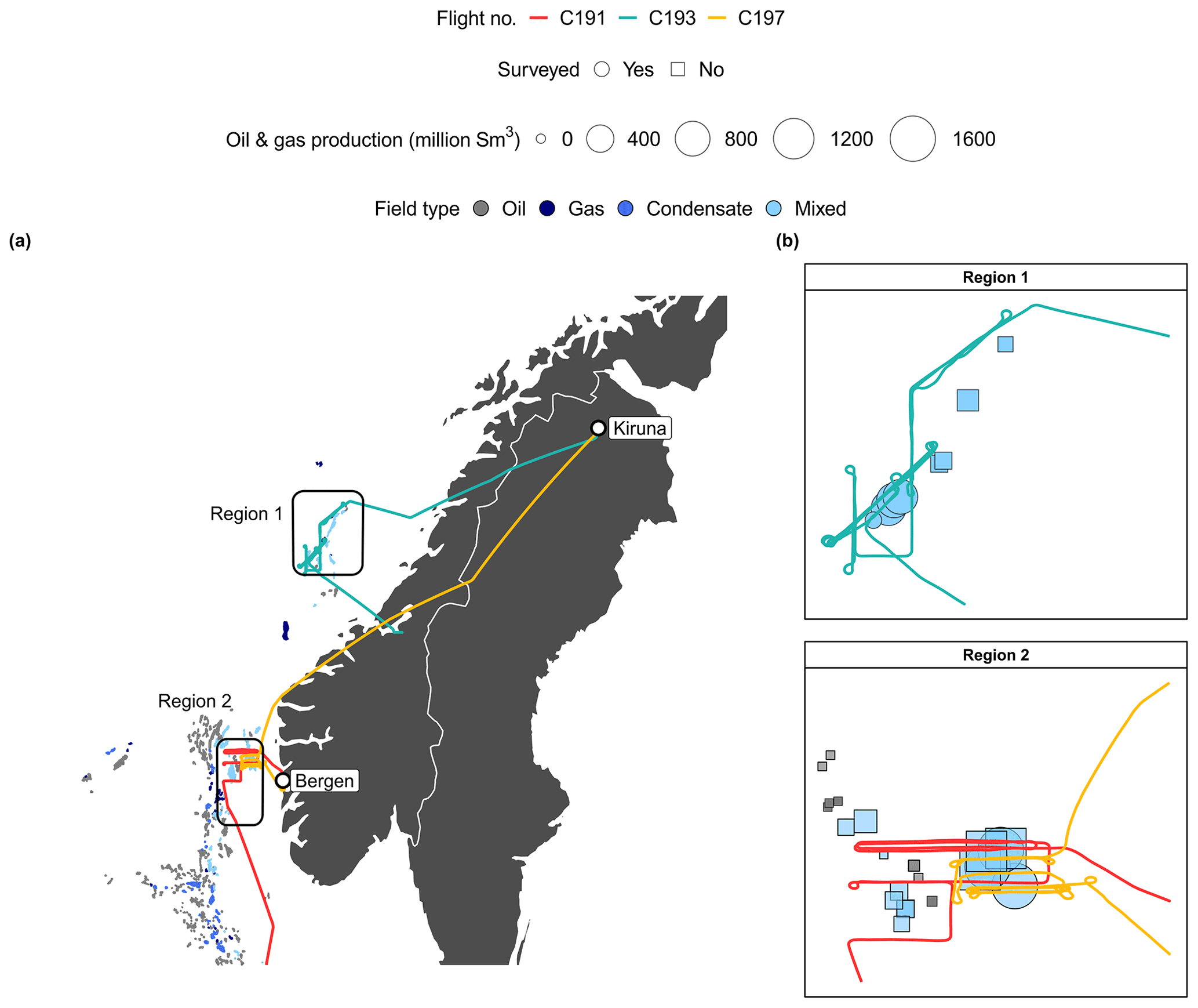
Figure 1 (a) Location of offshore fields on the Norwegian continental shelf and FAAM aircraft survey patterns (as coloured tracks). Each data point represents an offshore field, coloured by extraction product type (oil, gas, condensate or mixed). (b) Map of the FAAM flight tracks and locations of active O&G facilities in the two target regions. Each data point represents a distinct facility, sized according to the reported annual O&G production in 2019 (Norwegian Petroleum Directorate, 2021), with circles denoting facilities surveyed in this study. Sm³ refers to standard cubic metres.

During each of the FAAM survey flights, emissions from between two and four facilities were detected. These facilities were identified as the sources of the observed CH₄ plumes, using onboard wind direction and CH₄ measurements, alongside the GPS coordinates of the facilities. The atmospheric dispersion model FLEXPART was also used to aid source identification (Sect. 2.4).

The two regions were selected due to the large amount of oil and gas produced by facilities in each region, as seen in Fig. 1. Flight C191, in region 2, sampled between 134 and 370 m above sea level (m a.s.l.) with straight-and-level transects at 150 m a.s.l. upwind of the facilities to provide a representative background measurement. Repeated reciprocal runs at varying altitudes within the boundary layer were carried out downwind of sources to detect and characterise emission plumes. Flights C193 and C197 were conducted in regions 1 and 2, respectively. These flights involved two sets of vertically stacked transects at various altitudes. In flight C193, these transects ranged from 124 to 606 m a.s.l. with altitudes in flight C197 ranging from 103 to 308 m a.s.l. All three FAAM flights were conducted when the cloud base exceeded 300 m a.s.l. to ensure good visibility and allow for low-altitude sampling. Across the three flights, the number of stacked transects ranged from 7 to 14, at between 50 and 100 m spacing. See Appendix Fig. B2 for an example altitude–longitude projection of the stacked legs flown in flight C193. All three FAAM flights were conducted when the cloud base exceeded 300 m a.s.l. to ensure good visibility and allow for low-altitude sampling. There was no contact with the operators prior to or during the flights, where the operators were informed about the measurements. However, operators were aware of our study but not the time or the sampling pattern of the flights.

2.3.2 Scientific Aviation flights

Concentric closed flight laps were flown around each target site (individual facility), beginning at the lowest safe flight altitude (20 to 190 m a.s.l.) to an altitude exceeding the observed maximum emission plume height (typically 100 to 800 m a.s.l.), creating a virtual sampling cylinder incorporating both upwind background and downwind plume measurement. The number of laps varied for each facility surveyed, typically ranging between 5 and 25. See Appendix Fig. B3 for an example plot of one of these surveys. The highest altitude flown for each site was determined by the absence of significant upwind–downwind variability in the trace gas signal measured on board the aircraft (i.e. no downwind CH₄ enhancements were observed). The downwind lateral distance at which the plume was intercepted by the aircraft was typically 1–2 km.

The measurement sites were selected based on proximity to Bergen Airport, Norway, with facilities within approximately 200 km being investigated. Operators of target sites were informed of measurements on the common frequency for the local area during the flight itself. All airborne measurements were conducted under visual flight rules (VFR) flight conditions, meaning the aircraft was not flying in clouds, fog or low-visibility areas. This was done to ensure that a safe flying distance was maintained between the measured facilities and the sea surface.

Between two and eight facilities were surveyed on each of 10 survey flights conducted in August and September 2019. Over the course of the campaign, 21 O&G facilities were investigated (17 offshore facilities reported in Fig. 2), with repeated surveys of eight facilities over several days. The locations of the offshore O&G facilities surveyed during the Scientific Aviation flights are shown in Fig. 2.

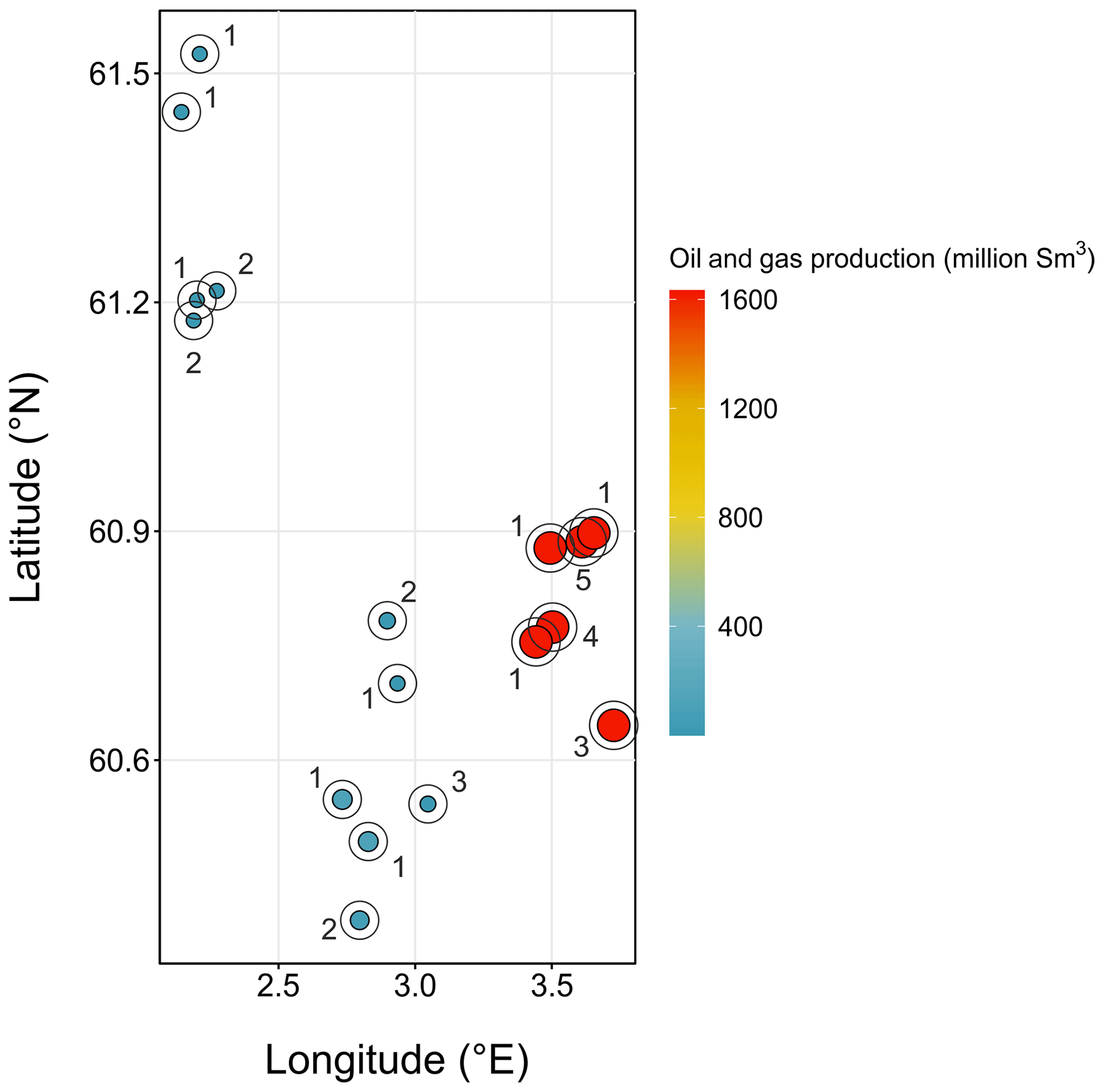
Figure 2 Location of the offshore O&G facilities sampled by the Scientific Aviation aircraft. Each platform is coloured and sized according to respective O&G production for 2019 (Norwegian Petroleum Directorate, 2021). Circles around each platform are used to illustrate the concentric flight laps conducted by the Scientific Aviation aircraft during sampling, with the numbers denoting the number of times each facility was surveyed. Sm³ refers to standard cubic metres.

2.4 Atmospheric dispersion model configuration

FLEXPART (FLEXible PARTicle dispersion model) is a Lagrangian dispersion model. FLEXPART was used to model the CH₄ emission plumes for target facilities. Backward plumes (or footprints) were also simulated, based on measured CH₄ data, to confirm the source facility of origin based on the locations of plumes sampled downwind during FAAM surveys. Source attribution was not necessary for Scientific Aviation surveys by virtue of the close proximity cylindrical sampling permitted by the smaller Mooney aircraft. FLEXPART simulates the Lagrangian trajectories of a large number of particles in the atmosphere. These particles, tracked forward or backward in time, were driven by Eulerian wind fields produced by the European Centre for Medium-Range Weather Forecast (ECMWF) with 0.1^∘ horizontal resolution and 137 vertical levels from the surface to approximately 80 km. The domain used was 0.0–12.0^∘ E, 57.0–68.0^∘ N.

Two different sets of simulations were performed: backward for source identification associated with individual airborne measurements and forward to aid the constraint of the maximum plume mixing height used for flux quantification (as described in Sect. 3). Backward plumes (or footprints) for every discrete measurement point were calculated along the flight tracks of FAAM flights C191, C193 and C197. For the backward simulations, the output grid resolution was $\mathrm{0.01}{}^{\circ }\times \mathrm{0.01}{}^{\circ }$ (∼1 km at the Equator) in the horizontal and 10 m in the vertical. Trajectories of 20 000 particles were calculated per individual measurement point. The footprint determined by the model was used to provide an estimated contribution from the facilities in question to the measured CH₄ enhancement at the point of measurement. This was then used to attribute the individual CH₄ plumes to specific facilities, based on the co-location of measured plumes. In addition, forward FLEXPART simulations were run, with output produced at the same resolution as the backward simulations, in order to estimate the maximum mixing height of the forward plumes emitted from the facilities on the Norwegian continental shelf. Example model data plots from both of these types of dispersion simulation can be found in Appendix A. A detailed description of the FLEXPART model and its components can be found in Pisso et al. (2019).

2.5 Reported emission data sources

2.5.1 Annualised CH₄ emission and activity data from platform operators

In Norway, facility-level reporting of offshore O&G CH₄ emissions is based on calculations at the source level using recommended guidelines (Norwegian Oil and Gas Association, 2018a), the results of which are then published (Norwegian Oil and Gas Association, 2021a). In this study, an inventory of existing O&G-related facilities in the study area as well as activity data including O&G production statistics and facility functions were obtained from public data sources (https://www.norskoljeoggass.no, last access: 29 September 2021, and https://www.norskeutslipp.no, last access: 29 September 2021). Additional data related to temporary facility activities such as flaring status or compressor ramp up for the days of the aerial surveys were provided via direct communication with the respective operators. Operators of facilities on the Norwegian continental shelf are required to submit annual CH₄ emission data to the Norwegian Environment Agency every year. The CH₄ emissions are reported for individual sources and subsources (e.g. primary vent seals for centrifugal compressors and incomplete combustion in flares). The basis for the reporting is a project led by the Norwegian Environment Agency between 2014 and 2016, which focusses on direct CH₄ emissions from O&G production activities on the Norwegian continental shelf (Husdal et al., 2016). All installations were subject to a detailed mapping of all potential sources of direct CH₄ emissions, and updated methodologies for quantifying emissions at the source/subsource level were established based on the best available techniques. The industry was an active participant in the project, and detailed recommended guidelines for emission and discharge reporting were established (Norwegian Oil and Gas Association, 2019). This was followed by a handbook for quantifying direct CH₄ and NMVOC emissions (Norwegian Oil and Gas Association, 2018b) and a guideline for the quantification of small leaks and fugitive emissions (Norwegian Oil and Gas Association, 2021b). The CH₄ reporting methodology on the Norwegian continental shelf is amongst the most advanced in the O&G industry globally, as each individual CH₄ emission source/subsource is configured at each installation (i.e. if gas is recycled, flared or cold vented). The detailed reporting associated with each facility is publicly available (Norwegian Oil and Gas Association, 2021c). This level of reporting is similar to Tier 3 Intergovernmental Panel on Climate Change (IPCC) guidelines (see Sect. 2.5.2). However, it should be noted that different countries and/or operators are likely to use different reporting procedures.

2.5.2 Global inventory of CH₄ emissions from oil and gas exploitation

Measured CH₄ emissions from individual facilities were compared with a regional sample of a global, gridded inventory of CH₄ emissions from oil, gas and coal exploitation with a resolution of 0.1^∘ × 0.1^∘ for the year 2016 (Scarpelli et al., 2020). The gridded inventory resolves contributions from individual subsectors (exploration, production, transport and refining) and from specific processes (flaring, venting and leakage). National emissions for each of these subsectors and processes were routinely compiled from UNFCCC national reported emissions using IPCC Tier 1 methods (IPCC, 2006). Such methods apply default emission factors (not country-specific) and activity data which are limited to national O&G activity statistics. These national emissions are then spatially allocated on the inventory's 0.1^∘ × 0.1^∘ grid across specific O&G infrastructure, in order to derive spatially aggregated emission estimates for infrastructure in each grid cell. The inventory therefore acts as a spatially downscaled representation of these UNFCCC reports. Higher-tier IPCC approaches are assumed to be much more rigorous and detailed. For example, Tier 2 approaches use country-specific emission factors. Tier 3 approaches apply a rigorous bottom-up assessment of emissions by primary source type (venting or flaring) using data reported by individual facilities (IPCC, 2006). This is a much more detailed and extensive process for compiling emissions. However, not all nations or facilities collect or report such data, meaning that it would not be an effective or consistent way to derive emissions for a global inventory. As discussed in Sect. 2.5.1, facility-level reporting of offshore O&G CH₄ emissions in Norway is based on calculations at the source level using recommended guidelines (Norwegian Oil and Gas Association, 2018a). In this context, the comparisons made in this study represent a comparison with a spatially downscaled estimation approach (Scarpelli et al., 2020, inventory) and the more detailed quantification approach used by O&G facility operators (facility-level reports).

Annualised gridded emission fields for O&G platforms for the year 2016 were downloaded from the Harvard Dataverse (Scarpelli et al., 2019). Equivalent inventory data for 2019 were not available at the time of the study. This is often a problem for inventory comparisons, as some inventories are not updated in real time, which can impact the accuracy of comparisons if changes in infrastructure may be expected in the intervening time. We include the comparison here as an illustration of this challenge. CH₄ emissions associated with the platforms of interest were extracted, using their geographical coordinates to identify the corresponding grid cell and CH₄ emission in the inventory.

3 Flux analysis methodology

In this section, we describe the flux quantification method applied to sampling from the FAAM and Mooney aircraft surveys and describe the quantification of flux uncertainty.

3.1 Aircraft mass balance

Fluxes can be quantified using mass balance approaches. For such approaches to be feasible, observations are typically made upwind of the source region, to establish concentrations in a background location. Downwind observations are then conducted, allowing for the determination of the net enhancement attributed to the source region. Lagrangian mass balance flux quantification typically requires meteorological conditions where the wind field can be assumed (and measured) to be relatively invariant over the spatial scales of plume sampling for a target emitter (Cambaliza et al., 2014; Pitt et al., 2019; Fiehn et al., 2020). Often, it is assumed that the plume is vertically well-mixed within some layer (usually the planetary boundary layer, PBL). The vertical mixing assumption also requires that measurements are taken sufficiently downwind of the emission source so that emissions have had time to fully mix. The aircraft mass balance approach used in this study has also been used to derive fluxes of trace gases from large area sources, such as agriculture, oil and gas fields and cities (e.g. White et al., 1976; Wratt et al., 2001; O'Shea et al., 2014; Peischl et al., 2016; Pitt et al., 2019), as well as for individual O&G facilities (e.g. Lee et al., 2018; Guha et al., 2020).

3.1.1 FAAM flights

The emission fluxes presented in Sect. 4 were calculated from the FAAM survey flight data using Eq. (1):

$$\begin{array}{}\text{(1)}& F=\underset{\mathrm{0}}{\overset{z_{\text{max}}}{\int }}\underset{A}{\overset{B}{\int }}(C_{ij}-C_{\mathrm{0}})n_{\text{air}}{U}_{\perp ij}\mathrm{d}x\mathrm{d}z,\end{array}$$

where F (g s⁻¹) is the flux for the emission source, A and B are the horizontal boundaries of the plume, z_max is the maximum plume height, C_ij is the dry mole fraction of CH₄ at each point in the plume, C₀ is the representative background dry mole fraction of CH₄, n_air is the molar air density, and U_⊥ij is the wind speed perpendicular to the reference measurement sampling plane. For the flux calculations in this study, the atmosphere was divided into discrete vertical layers, based on the mean altitudes of aircraft transects for each facility survey. The mean concentrations within each observed CH₄ plume were used to calculate flux individually for each layer and summed across all layers to obtain total flux.

Representative background CH₄ mole fractions were determined for each layer using the 50 neighbouring 10 Hz measurements to either side of the observed plume. The average CH₄ enhancement above this background was calculated for each observed plume. The perpendicular wind speed was calculated as the average wind vector component perpendicular to each flight transect. Plume mixing altitude was calculated as the distance between the sea surface and either the point at which a plume was no longer observed in measured data or the height of the mixed layer as diagnosed from FLEXPART forward modelling or the nearest available potential temperature profile measured by the aircraft. In the absence of a direct measurement of plume mixing height, where the boundary layer height or FLEXPART model mixing was used to define the plume mixing height, the difference between the nearest altitude where a plume was measured and the assumed mixing height was used to define a quantifiable vertical mixing uncertainty used in flux error propagation (see Sect. 3.2). In summary, for surveys where the plume top could not be directly constrained by measurement, any assumed vertical mixing was conservatively accounted for within the quoted flux uncertainty reported in Sect. 4.

3.1.2 Scientific Aviation flights

A variant of the Lagrangian mass balance method, utilising Gauss's theorem and suited to the orbital sampling conducted by the Mooney aircraft, was used to derive CH₄ fluxes from the Scientific Aviation flight surveys. Gauss's theorem was used to estimate CH₄ flux through the virtual cylinder created by flying concentric circles around an individual platform. This theorem equates the volume integral of the source (e.g. platform) to a surface integral of the trace mass flux which is normal to the surface of a cylinder. The volume integral was converted to a surface integral, which was used to calculate the horizontal mass flow of CH₄ across the cylinder's surface plane. All other flux parameters in Eq. (1) were calculated in the same way as for the FAAM flight surveys. A full description of this emission quantification method can be found in Conley et al. (2017).

3.2 Flux uncertainties

3.2.1 FAAM flights

The uncertainty in the measured flux was determined using a method similar to that used by O'Shea et al. (2014). This involves propagating the measured uncertainties associated with the individual terms in Eq. (1), including the uncertainty in the observed CH₄ enhancement, the natural (measured) variability of the wind field and any uncertainty in the plume mixing height. Instrumental uncertainties associated with the FGGA were calculated to be negligible in comparison to those associated with the wind field and plume mixing height but are implicitly accounted for within the measured variability (and hence uncertainty) in the background concentration.

Non-correlated, random uncertainties (wind and background variability) were summed in quadrature and calculated as an uncertainty for each altitude layer. These were then summed for all altitude layers to derive an overall random uncertainty in the corresponding total flux. The systematic uncertainty in the plume mixing height (described in Sect. 3.1.1) was then added to the random error to obtain the total uncertainty in the flux reported for each facility.

3.2.2 Scientific Aviation flights

The uncertainties in emission flux (reported as an uncertainty of 1 standard deviation) were calculated as follows and are analogous to those calculated for FAAM survey data. Firstly, the statistical (random) uncertainty in the wind field and the CH₄ measurement from the Picarro instrument were summed in quadrature, in order to obtain uncertainty in the horizontal flux for each concentric lap. The horizontal fluxes were then binned in altitude layers, and the uncertainties of the horizontal fluxes in that bin were summed in quadrature along with the standard deviation of the flux estimates for each layer. The uncertainties in each bin were added in quadrature to obtain the final error estimate for the total flux measurement for each individual survey.

Where multiple surveys were conducted over several days, this was taken into consideration when calculating the overall uncertainty for each facility. The relative error for each survey was calculated. These were then averaged to give a mean uncertainty over all surveys for each facility. The mean relative uncertainty was then multiplied by the average CH₄ flux to obtain a mean-weighted uncertainty in the CH₄ flux for each facility.

4 Results and discussion

In this section, we report the measured fluxes for each facility and compare with inventory and facility-level activity data. Details about the observational data from the FAAM and Scientific Aviation flight surveys and the application of the mass balance approach can be found in Appendix B.

4.1 Measured flux uncertainties

Uncertainties in flux are a function of sampling density, background variability and wind conditions, as well as the instrumental uncertainty (France et al., 2021). Combined uncertainties associated with background and wind variability were observed to be less than 10 % in the FAAM flight surveys of this case study. The largest source of flux uncertainty in the FAAM flight surveys was found to be in the plume mixing height (typically accounting for more than 90 %). As discussed in Sect. 3.1.1, this was calculated as either the height at which a plume (CH₄ enhancement) was no longer observed downwind or, in the absence of a vertical measurement constraint, as the nearest available measured thermodynamic boundary layer height as a proxy for maximum possible mixing. The vertical plume was more constrained by the Scientific Aviation flight patterns due to the dense vertical sampling made possible by the more agile, smaller Mooney aircraft, reflected by the smaller flux uncertainties in the Scientific Aviation surveys (see Table 1). However, there is also some additional uncertainty if the bottom of the plume cannot be sampled. This is captured in the uncertainties reported for all flights and represents an inherent limitation of all aircraft surveys. By the way of forward guidance, an optimal sampling design (to minimise flux uncertainty) therefore involves repeated sampling at many altitudes around a target of interest, ensuring that the top of any plume is directly measured.

4.2 Flux comparisons with a global inventory and facility-level reported data

This study involves direct comparisons of the measured CH₄ fluxes with those reported by facility operators and global emission inventory estimates. This requires temporal unit conversions of the measured data (from g s⁻¹ and kg h⁻¹ to t yr⁻¹). Scaling in this way is likely not to be a robust comparison, as it cannot account for any variability in day-to-day facility operations throughout the year. Such day-to-day variability has also been observed and discussed in Tullos et al. (2021), whereby short-duration CH₄ measurements were made at 33 dry-gas production sites in eastern Texas over the course of 3 weeks. This study demonstrated that observations made at the same sites, within days of each other, could result in very different emission estimates. However, as it is impractical to quantify the emissions from the facilities every day of the year, flight surveys provide us with “snapshots” of the emissions, scaled to annualised data for direct comparisons, and yield insights into the sources of any observed discrepancies, especially when comparing a large number of surveys and facilities in aggregate. This annualised approach has been used to compare inventories with discrete measurement surveys of offshore O&G facilities, as discussed in Sect. 1.

Figure 3 shows the spatially gridded CH₄ estimated emission data from the Scarpelli et al. (2020) global inventory for the Norwegian continental shelf. The estimated emissions shown represent those sourced from fuel exploitation (i.e. oil, gas and coal) for the year 2016. The highest estimated emissions in the area of interest range from approximately 1.6 to 2.0 $\mathrm{t}{\mathrm{CH}}_{\mathrm{4}}{\mathrm{yr}}^{-\mathrm{1}}{\mathrm{km}}^{-\mathrm{2}}$, and it is these data which are used to compare against the measured CH₄ fluxes from the aircraft surveys in this study. We recognise that the emissions derived from this inventory are estimates for the individual facilities surveyed in this study and do not reflect what is reported by operators. Inventory estimates such as these are not used as the basis for national emission reporting.

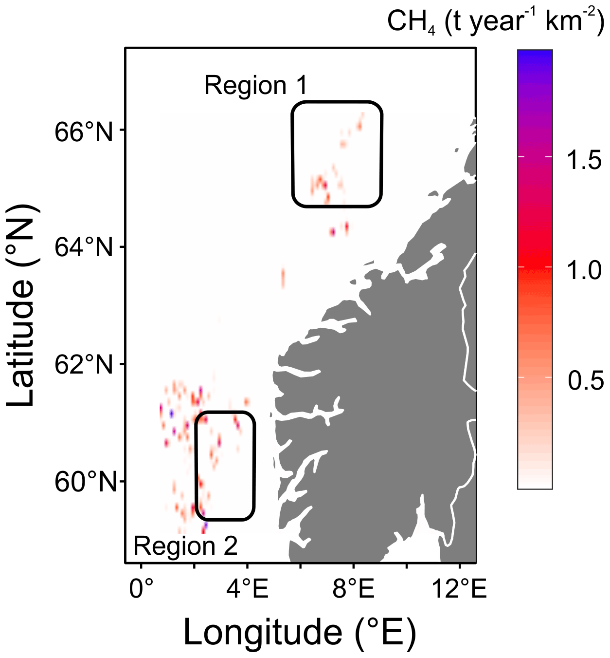
Figure 3 Spatially gridded CH₄ emissions from fuel exploitation for the northern North Sea and Norwegian Sea (Scarpelli et al., 2020). Regions surveyed in this study are represented by the boxes labelled “Region 1” and “Region 2”.

Figure 4a displays the measured CH₄ emission fluxes and corresponding spatially downscaled inventory estimates for all of the offshore O&G facilities surveyed in this study. Measured CH₄ emissions are reported in units of tonnes per year in order to ensure consistency with the units used in the emission inventory and facility-level reported data. The inventory contains significantly underestimated emissions for facility 2 (seen as the outlier in Fig. 4a with an inventory flux of ∼60 t yr⁻¹), with measured CH₄ emission fluxes over a factor of 20 higher, whilst also noting that the measured flux uncertainty was high. However, considering the low R² value (0.02) in Fig. 4a, we emphasise that the intercepts and gradients calculated in this regression analysis are not meaningful, due to the high variability of agreements amongst the individual facilities. We include the result here to make this valuable point, which is to say that the downscaling of inventories can lead to significant discrepancies at the scale of oil and gas facilities, such as those studied here.

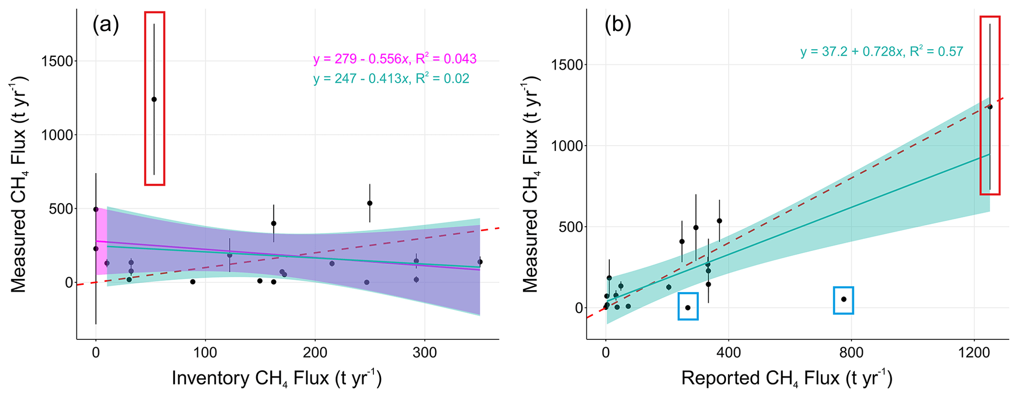
Figure 4 Comparison of measured CH₄ emission fluxes and (a) corresponding estimates from the Scarpelli et al. (2020) global inventory and (b) corresponding operator-reported emissions for each facility. The data point in the red box represents a particularly high measured flux of 1239.65 t yr⁻¹. The data points in the blue boxes in panel (b) represent the two facilities which do not fit with the general pattern, with near-zero measured fluxes. The green line represents a fitted linear regression through all data points, and the magenta line represents a fitted regression which excludes inventory or reported emissions of zero. This magenta line is not shown in panel (b), as the two regression lines were essentially identical. The font colours of the equations shown correspond to the colour of the respective regression line. The shaded regions of these lines correspond to the 95 % confidence levels for the slopes. The red dashed line shows the 1:1 correspondence line for illustration.

Figure 4b compares the measured emission flux with facility-level reported emissions, which have similarities with Tier 3 emission reporting. This figure shows a much closer agreement than that observed in Fig. 4a, with an improvement in the number of facilities falling within the 95 % confidence interval of the fitted regression between the measured and reported emission flux. Figure 4b shows two facilities that do not fit the pattern (within uncertainty), with reported fluxes of 270 and 780 t yr⁻¹. These correspond to facilities 20 and 17, respectively, with significantly smaller measured emission fluxes. These results from these two facilities demonstrate how inventory guidelines need to be improved to ensure more consistency with operations. A near-zero measured emission flux was reported for facility 20. This is consistent with temporary inactivity, resulting from turbine maintenance on this O&G facility reported on the day of the flight survey. Correspondence with operators of facility 17 highlighted the fact that the cold vent is located in close proximity to the ignited flares, meaning that some CH₄ gas may be combusted as it passes near to the flare. This would not be implicitly accounted for in the reported fluxes for this facility, which assume that all cold-vented gas is emitted directly, without any combustion taking place. Consequently, this could result in an under-bias in the reported emission fluxes and hence the observed discrepancy when compared with the measured emission fluxes for facility 17. The nature of cold venting and the potential for combustion therefore represents a potential problem for accurate CH₄ emission reporting.

The regression in Fig. 4b does not include reported emissions of zero, as shown in Fig. 4a, as the two regression lines were found to be essentially identical. These results show that in aggregate, with a sufficient number of surveys, measurements are able to replicate the facility-level reported emissions whilst also confirming that facility-level reporting procedures can provide accurate emission estimates for the incorporation into inventories. Facility 2 (the outlier seen in Fig. 4a, discussed above) shows good agreement between operator-reported emissions and measured data, suggesting that facility-level reported flux for facility 2 is much more accurate than that represented by the inventory and therefore that the observed difference between the measured and inventory emission estimates can be attributed to the emission calculation methodology applied in the inventory. This is consistent with the conclusions of other studies that have compared top-down measurements and global inventories compiled using the Tier 1 approach (Sect. 2.5.2; Gorchov Negron et al., 2020; Zavala-Araiza et al., 2021).

Table 1 compares the measured CH₄ emission fluxes with both annualised facility-level fluxes reported by respective facility operators (using approaches similar to those applied in IPCC Tier 3 emission quantification approaches) and corresponding emission estimates from the Scarpelli et al. (2020) global emission inventory (compiled using the IPCC Tier 1 approach). Due to commercial sensitivity, the platforms are arbitrarily labelled with a number in Table 1, and the operators are not identified. Facilities 6 and 7 were surveyed separately by the aircraft. However, the reported emissions were grouped for the two facilities, which impedes our ability to directly compare to the reported flux for each facility separately. However, our observations show that emissions were dominated by facility 6 (400 t yr⁻¹) relative to facility 7 (9.6 t yr⁻¹). For individual facilities, there are notable large differences between the inventory estimates and the extrapolated measured emission fluxes, ranging from −41 % (−88 t yr⁻¹) to 2200 % (1200 t yr⁻¹) for facilities 5 and 2, respectively. This is expected to be associated with both the compilation methodology of the inventory, whereby national emissions are downscaled to corresponding infrastructure, and the fact that the Scarpelli et al. (2020) inventory was compiled for the year 2016. The latter was due to equivalent inventory data for 2019 not being available at the time of this study, thus illustrating the challenge of inventory comparisons, with respect to infrastructure changes which may take place in the intervening time period between the inventory compilation and the surveys.

Table 1 Summary of the measured CH₄ fluxes and comparison with respective emission data from the Scarpelli et al. (2020) global inventory and reported CH₄ emissions from the O&G facility operators. All measured, reported and Scarpelli et al. (2020) inventory (Scarpelli inventory) fluxes are quoted to two significant figures here. Flux uncertainties represent confidence intervals of 1 standard deviation for each facility (see Sect. 3.2 for details). SA: Scientific Aviation.

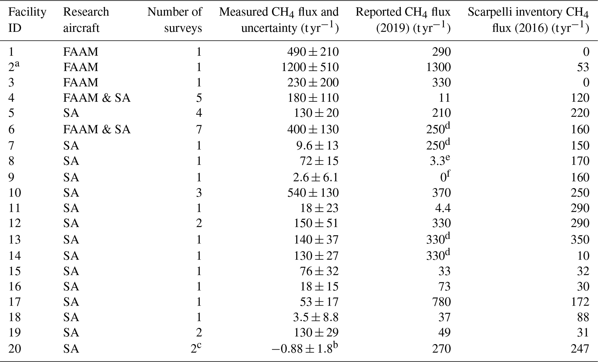
^a Collective ID for two facilities to coincide with grouping in inventory and reported estimates. ^b The relatively low absolute mean flux with a negative sign is an artefact of minor upwind CH₄ contamination overwhelming the downwind CH₄ enhancement. It is acknowledged that physical CH₄ emissions from this facility cannot be negative. ^c Facility was surveyed twice. Only one measured flux is reported, as upwind contamination invalidated the second measurement. ^d Both facilities were measured separately, but the operator reported a combined estimate. ^e Facility is a subsea manifold station. A drilling vessel was drilling at the same location at the time of surveying. The operator reported that drilling was the main CH₄ source of >99 % of CH₄ emissions and that CH₄ emissions will only occur during drilling. ^f Operator did not report emissions, as this facility was reported inactive during 2019.

Global inventories such as these do not have the granularity or detail compared with that provided by operator-reported data for individual facilities (see Sect. 4.3). Such large differences between top-down methods and emission inventories have been reported previously (see Sect. 1). Gorchov Negron et al. (2020) compared regional airborne estimates of CH₄ emissions from offshore O&G facilities in the Gulf of Mexico with the US Environmental Protection Agency greenhouse gas inventory, with measured CH₄ emissions found to be consistent for deep-water but a factor of 2 higher for shallow-water facilities.

Considering all facilities collectively, the measured fluxes were found to be 42 % greater than the Scarpelli et al. (2020) emission inventory using Tier 1 methods. However, there is a much-improved agreement in comparison with the facility-level reported flux where measured fluxes are 16 % lower than those reported. This aggregated comparison with facility-level reported data suggests that measurements and reported data agree within uncertainty, given a large enough sample size, and therefore we recommend that facility-level reporting be adopted more widely and used to compile more robust inventories of CH₄ emissions. As discussed earlier, the Scarpelli et al. (2020) inventory was compiled for 2016, as equivalent 2019 data were unavailable at the time of this study. Using a scale factor, derived as a ratio between the 2016 and 2019 total reported emission data from the offshore fields (Norwegian Oil and Gas Association, 2021a), we can proportionally scale 2016 inventory estimates to better represent 2019 when comparing measured emissions to the Scarpelli et al. (2020) inventory. Repeating the analysis above, using the scaled Scarpelli et al. (2020) inventory, we find that total measured emissions were 52 % higher than the inventory for 2019. This further highlights the limitation of comparisons with global inventories and their Tier 1 approach and shows that a better agreement can be observed in comparison with a more specific inventory (e.g. facility-level reported emissions). Therefore, the poorer agreement between the measured fluxes and the Scarpelli et al. (2020) inventory can be interpreted to reflect the representativity of the inventory, due to its construction methodology and the fact that it was compiled for 2016 (and thus is not representative of emissions in 2019), rather than a systematic error in the operator-reported emissions, which agree with the measured fluxes.

4.3 The relevance of platform operational data and CH₄ loss rate calculations

Figure 5 displays a summary of facility-level CH₄ emission estimates including repeat measurements. Hourly emission rates were annually extrapolated for comparison with reported values. Panel a groups the facility IDs into three clusters. The first cluster (IDs 4–7) contains facilities for which measurements were available under both “primary” operations and “other” operations. Primary operations are defined as operations which are central to the production of hydrocarbons and which emit CH₄ almost continuously in the context of this study. Other operations are defined as temporal deviations from the primary operations (based on operator reports received upon request after the campaign), which may increase or decrease snapshot emission estimates relative to annualised inventories (see details below). The second cluster (IDs 1–3, 10, 11, 13–17 and 19) contains facilities for which measurements were available only under primary facility operations. The third cluster (IDs 8, 12, 18 and 20) contains facilities for which measurements were available only under other facility operations. Panel b shows the total facility emissions, which is based on average facility emissions for repeated surveys. The first column represents only the first cluster from panel a. The second column represents only the second cluster from panel a. The third column represents all facilities from panel a, i.e. a mix of primary and other operations. The facility-level uncertainties shown by the error bars in Fig. 5 were propagated in panel b using a Monte Carlo simulation, assuming normally distributed errors and independent samples. The latter is based on the fact that repeat sampling occurred on different days and that individual platforms operate independently of one another.

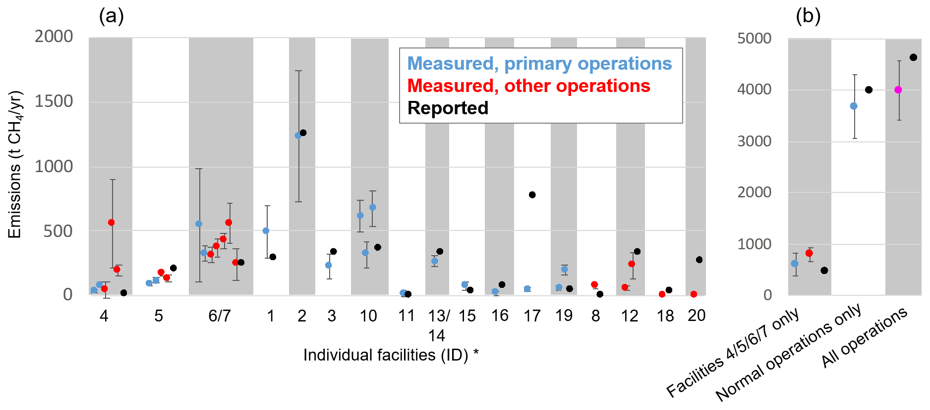
Figure 5 Facility-level CH₄ emissions (multiple data points per facility represent repeat surveys on different days). (a) Measured (red and blue) and facility-reported (black) CH₄ emission estimates by facility ID number. (b) Total emissions (based on average facility emissions for repeated surveys). The first column includes only facilities 4, 5, 6 and 7 (representing “other” operations). The second column represents all other facilities (representing “primary” operations). The third column represents all facilities collectively (magenta data point). Error bars represent 1σ uncertainties. ^∗ Facilities 6 and 7 and 13 and 14 were measured separately (and fluxes were added), but the operator reported a combined estimate. Facility 9 is not included here because it was reported inactive during 2019 and because measured CH₄ emissions were negligible (see Table 1).

As shown in Fig. 5a, operator-reported facility-level, annualised emission rates agree with single survey measurements within uncertainties for 24 % of the offshore surveys. However, for 76 % of the surveys, reported emissions underestimate or overestimate measured values at individual facilities independently of whether the facilities were surveyed under primary (continuous) operations or other operations. Other operations include facility turnaround, turbine/compressor irregularities (such as lower-than-usual turbine load, compressor out of operation, or compressor ramp up and shutdown), reduced gas production or routing to a connected facility, increased flaring, and well drilling. The operation report descriptions thus suggest that other operations are expected to lead to either increased or decreased emissions relative to the annual average emissions. Indeed, the measurements confirm this expectation (reported emissions tend to underestimate measurements at facilities 4, 6 and 7, and 8 and overestimate at facilities 5, 12, 18 and 20). Reported emissions almost equally underestimate (facility 4) or overestimate (facility 5) emissions even if there is agreement with measurements on other survey days. Keep in mind that the operator-reported annualised emissions account for both primary and other operations throughout the year. Consequently, the robustness of a top-down vs. bottom-up comparison for an individual facility increases with more frequent sampling.

Note that at the five facilities with repeat surveys on different days under primary operations (blue dots at facility IDs 4, 5, 6, 10 and 19 in Fig. 5a), the average day-to-day variability in measured emissions for the same facility is 33 % (even after accounting for measurement uncertainties). That is, emissions at the same facility vary substantially over time, even on days when the operational status suggests continuous emissions. This implies that intermittency exists beyond the granularity (or the categories) of the level of reporting above. Nevertheless, as shown in Fig. 5b, at the aggregate level of 19 facilities (34 surveys including repeats; number is slightly different from column 5 in Table 1, which separates facilities reported jointly), reported emissions agree with average measurement-based fluxes within 16 % irrespective of operating status (rightmost column of Fig. 5b, just outside the 1σ error). When considering only primary operations, this difference is only 8 % (middle column of Fig. 5b, with 1σ error). The direct comparison of measurements during primary and other operations at facilities 4, 5, and 6 and 7 indicates that average emissions during other operations are 29 % larger than during primary operations for these facilities, although this difference is largely driven by one outlier in facility 4. It is noteworthy that the majority of the randomly timed surveys (10 out of 16 surveys) at facilities 4, 5, and 6 and 7 occurred during other operations. Considering all 20 surveyed facilities, 15 out of the randomly timed 34 surveys were under other operations. As such, an annual extrapolation of only the measurements under primary operations would substantially underestimate annual emissions given the frequent occurrence of other operations. While accounting for the operational status will be key for prioritising emission mitigation solutions, our results suggest that randomised but intensive field-specific surveys remain the key driver of sampling required to deliver unbiased estimates of total emissions at the facility level (repeat surveys) or the regional level (multi-facility surveys), irrespective of operational status. While the cost of the surveys and the monetary and environmental benefits play a role in designing routine surveys, frequent surveys could ensure the most robust validation.

We further calculated CH₄ loss rates, i.e. the measured, annualised CH₄ emissions as a fraction of the marketed CH₄ over the same period. This was conducted at the field level (for which gas production data were available; Norwegian Petroleum Directorate, 2021), which includes between one and six individual facilities depending on the field. NOGA (2018) guidelines were used to approximate gas composition to convert total gas production (Norwegian Petroleum Directorate, 2021) to CH₄ production. Measured CH₄ loss rates range between 0.003 % and 1.3 %, thus spanning 3 orders of magnitude. This wide range in loss rates is largely driven by the equally wide range in gas production across the 10 fields, spanning 4 orders of magnitude. While there is no apparent correlation between absolute emission rates and leak rates, all four fields with loss rates >0.1 % each produce $<\mathrm{0.15}\times {\mathrm{10}}^{\mathrm{9}}$ Sm³ (standard cubic metres, i.e. volume at standard atmospheric temperature and pressure), and all six fields with loss rates <0.1 % each produce $>\mathrm{0.5}\times {\mathrm{10}}^{\mathrm{9}}$ Sm³. Thus, the very small loss rates <0.1 % are largely explained by the large denominator (gas production volume). The gas production-weighted average loss rate for the 10 measured fields is 0.012 %, but this value should not be considered representative of Norwegian offshore production, and it is very likely a conservative estimate for the full population of Norwegian sites. This is because the 10 measured fields in this study account for 48 % of Norwegian gas production but for only 12 % of the total number of producing fields (Norwegian Petroleum Directorate, 2021). In other words, measured fields in this study are strongly biased toward high gas production fields, which in turn explains the relatively small weighted average loss rate.

4.4 Outlook

In summary, these results act as a comparison of top-down measurement-based emission quantification, bottom-up facility-specific calculations (similar to the IPCC Tier 3 approaches; IPCC, 2006, 2019) and bottom-up IPCC Tier 1 calculations using generic emission factors (used in Scarpelli et al., 2020). As outlined in Sect. 2.5.2., Tier 3 approaches are more rigorous and detailed, applying facility-level emission and activity data to calculate emissions. Results in this study show that there is better agreement between measured data and facility-level reported emissions than more generalised spatially downscaled inventory estimates, as expected. This result emphasises the importance of facility-level emissions reporting in order to compile accurate national greenhouse gas inventories. This study exclusively considers offshore O&G facilities, adding to the findings from previous work which found that spatially downscaled inventories may be significantly underestimating CH₄ emissions (Gorchov Negron et al., 2020). However, other studies have also observed discrepancies in inventory estimates for onshore facilities (Zavala-Araiza et al., 2021), thus highlighting that Tier 1 inventories can be subject to very high inaccuracy across the O&G sector as a whole.

In this context, it is important that the availability of Tier 3 reported data is increased and more routinely required by regulators and policymakers and that such data are used to more meaningfully inform overall IPCC emission scenarios, which may currently contain large underestimates for the offshore O&G sector where only spatially downscaled estimates are available. This represents both a global and field-specific challenge, as individual basins typically comprise multiple operators with potentially different performance standards and reporting frameworks. There is an urgent need for consistent, internationally agreed standards of best practice, if reported fluxes are to be of value in accurately understanding global emissions from the O&G sector.

Additional measurements are needed to further test and validate global emission inventories. However, collecting such data is labour-intensive and, thus, expensive when using manned aircraft. Slow-moving, lightweight airborne measurement platforms, such as the Mooney aircraft are well-suited to this application, as they allow for much more focussed sampling, with the ability to densely sample in close proximity to individual O&G facilities. However, future improvements and advances in satellite remote sensing could provide routine datasets to assess facility-level and area emission reporting, providing greater spatial and temporal coverage. However, flux measurements in the offshore environment via satellite remote sensing are challenging due to the use of less frequent glint mode observations (for passive near-infrared sensors). Other survey platforms, such as unmanned aerial vehicles (UAVs) also offer the potential for CH₄ flux quantification from numerous sources (e.g. Nathan et al., 2015; Yang et al., 2018; Allen et al., 2019; Shah et al., 2020; Shaw et al., 2021). For an interesting overview of CH₄ detection technologies for offshore environments, see Carbon Limits (2020). Frequent surveys could lead to measurement-based inventories, similar to that compiled by Gorchov Negron et al. (2020), as efforts continue to quantify emissions and seek to combat global climate change.

5 Conclusions

This study reports CH₄ fluxes derived from airborne sampling campaigns on the Norwegian continental shelf. We conducted 13 flights using the FAAM and the Scientific Aviation research aircraft in July, August, and September 2019.

Measured CH₄ emissions were found to range from 2.6 to 1200 t yr⁻¹ (with a mean of 211 t yr⁻¹ across all 21 facilities). Mean measured fluxes (as an aggregate of the 21 facilities studied) were 16 % lower than equivalent operator-reported data but agreed within 1σ uncertainty. Operator-reported emission data contain an increased level of granularity concerning operational emissions and sources, better representing the reported facilities, relative to IPCC Tier 1 data used in the global inventory, making it more closely analogous to IPCC Tier 3 methods. Measured CH₄ emission loss rates (as a percentage of CH₄ production) ranged from 0.003 % to 1.3 % across facilities, with the wide range largely driven by field-level production volumes, with high-producing fields displaying proportionately lower emission rates. The aggregated comparison with facility-level reported data suggests that measurements and reported data agree within uncertainty. With this in mind, we recommend that similar facility-level reporting is adopted more widely by industry and that reported data are used to more accurately compile national emission inventories of CH₄ relevant to IPCC emission scenarios. This reporting approach is consistent with the voluntary commitment required for membership in the Oil and Gas Methane Partnership 2.0.

We also compared aircraft-derived fluxes with facility fluxes extracted from a global gridded fossil fuel CH₄ emission inventory, finding that the measured emissions were 42 % larger than the inventory for the 21 facilities surveyed (in aggregate). We interpret this large discrepancy to reflect not a systematic error in the operator-reported emissions, which agree with measurements, but rather the representativity of the global inventory due to the methodology used to construct it and the fact that the inventory was compiled for 2016 (and thus not representative of emissions in 2019). This highlights the need for timely and up-to-date inventories for use in research and policy.

This study also demonstrates the use of airborne sampling to obtain flux snapshots for comparison with inventories and reported data. We found that measurement sampling density, especially in the vertical plane, can dominate sources of uncertainty in aircraft-based flux methods. To reduce uncertainty in flux calculations further using measurement-based approaches, we recommend the use of measurement platforms with a high degree of manoeuvrability.

Appendix A: FLEXPART dispersion model: example forward and backward simulations

Figure A1 shows an example curtain plot for flight C193. Such plots were constructed from the forward simulations of the FLEXPART model for FAAM flights C191, C193 and C197, in order to estimate the modelled plume height. The release of a unit mass from selected rig locations yields 4-dimensional FLEXPART output (in e.g. ppb) and provides the basis for interpolation along and below/above the flight track. The derived PBL height is generally consistent with flight data. The forward FLEXPART simulations were based on regional ECMWF winds, which were retrieved specifically for this application. Their domain is 0–12^∘ E, 57–68^∘ N, with 137 hybrid levels. The winds were natively interpolated at 0.1^∘ horizontally. The runs were performed with high temporal resolution, with a synchronisation time (internal FLEXPART time step) of 50 s. The turbulence in the planetary boundary layer was parameterised with refined horizontal and vertical Lagrangian timescales, represented by the FLEXPART parameters of CTL=40 and IFINE=10 (for definitions of these abbreviations, see Table 8 of Pisso et al., 2019). The gridded output resolution is 0.01^∘ with domains containing the flight track and the targeted rigs. The time step of the gridded output for the plumes is 50 s (FLEXPART parameter LOUTSAMPLE) averaged over 1 h (FLEXPART parameters LOUTSTEP and LOUTAVER set to 3600).

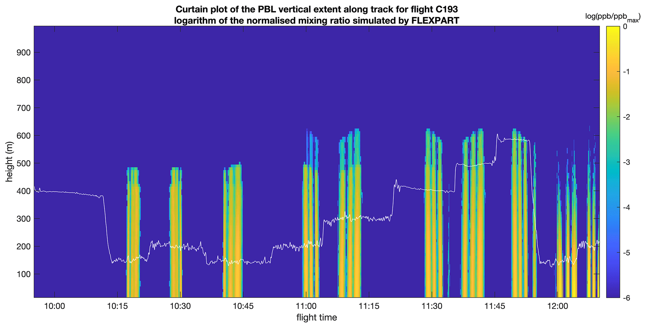
Figure A1 Example curtain plot for the forward FLEXPART simulation for FAAM flight C193 used to estimate modelled plume height. The white line denotes the flight altitude, and the shaded area denotes the logarithm of the normalised volume mixing ratio of CH₄ (column containing each measurement).

Figure A2 shows an example modelled footprint for flight C193, based on backward trajectories simulated by the FLEXPART model. These simulations were conducted for FAAM flights C191, C193 and C197. The calculation of retroplumes (or “footprints”) for each data point along a flight track allows for the identification of oil and gas platforms linked to individual peaks detected in the time series of measured CH₄. The magnitude of the retroplume is proportional to the time averaged spent by trajectories in the corresponding grid cell.

Figure A2 Example snapshot of the calculated FLEXPART footprint for FAAM flight C193 used to aid source identification for measured CH₄ enhancements. The flight track is coloured by the measured CH₄ mixing ratio (right colour bar; ppbv). The shaded area denotes the vertically integrated retroplume (left colour bar; s m² kg⁻¹). The red triangles represent the locations of the nearby offshore O&G facilities.

Appendix B: Aircraft observational data

Figure B1 shows the flight track of FAAM flight C193, which took place on 30 July 2019, along with nearby offshore O&G facilities. Figure B1a shows the measured wind speed and direction (shown as arrows), and Fig. B1b shows the measured CH₄ mole fraction. The FAAM measurement data in Fig. B1 showed CH₄ enhancements above background of between approximately 2 and 13 ppb. However, much larger enhancements were seen in region 2 overall, with a maximum of 99.3 ppb above background. A maximum of 8.9 ppb was observed in region 1. This was as expected as the facilities in region 2 were known to produce substantially more oil and gas compared to region 1, as seen in Fig. 1 in Sect. 2.3 of the main paper.

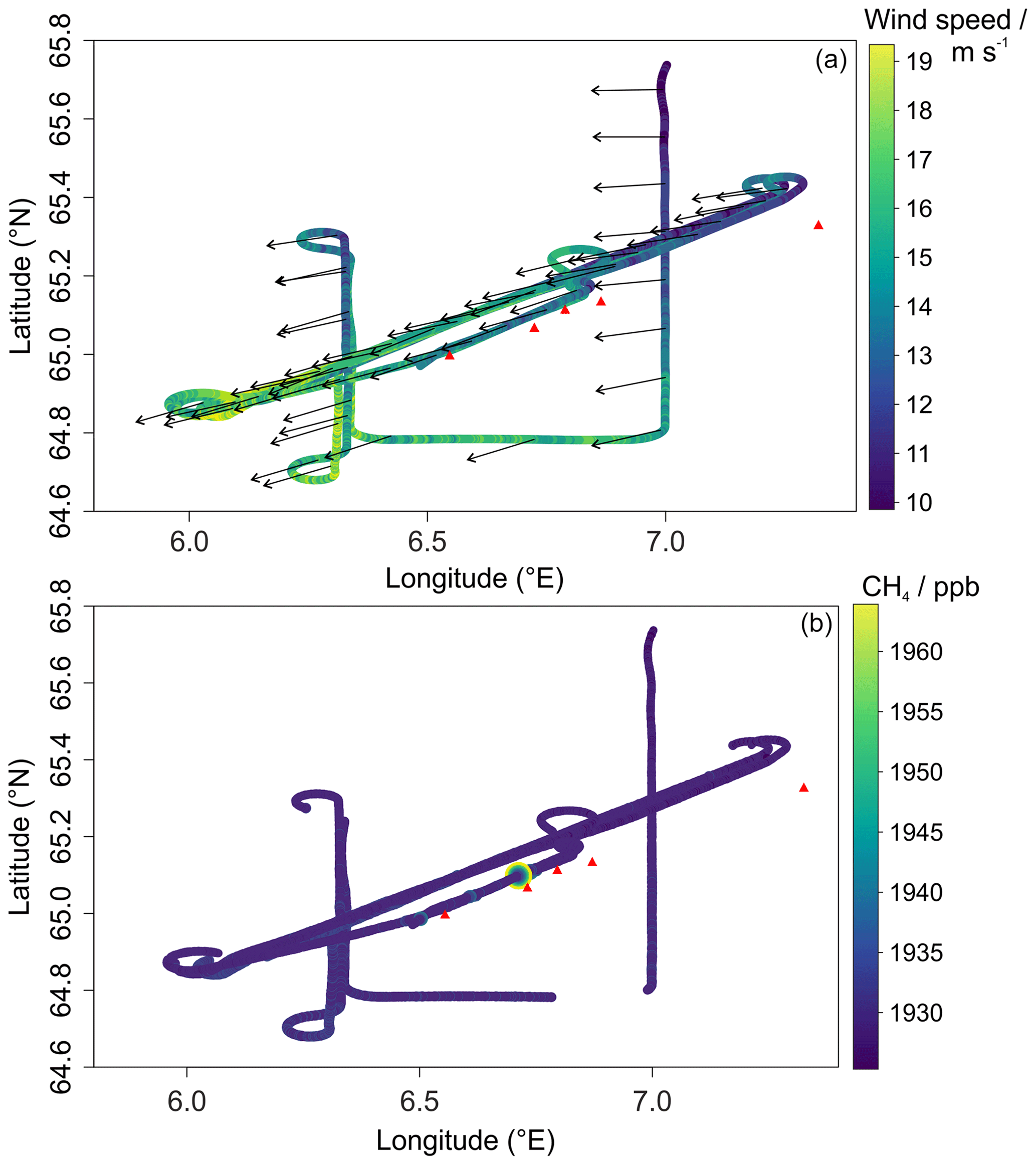
Figure B1 Flight track for flight C193, (a) colour-coded by the wind speed, with arrows denoting the wind direction over the course of the flight, and (b) colour-coded by the CH₄ mixing ratios. The red triangles represent the locations of nearby offshore O&G facilities.

Figure B2 shows the altitude–longitude projection of the vertically stacked transects from flight C193, as an example. During the flight, seven transects were flown downwind of the offshore facilities, with a spacing of between 50 and 100 m between each transect. Flights C191 and C197 comprised 7 and 14 vertically stacked legs, respectively, with a spacing of between 50 and 100 m between each transect.

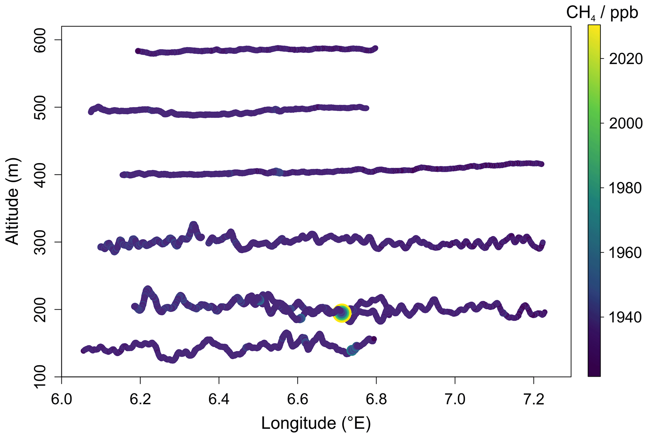
Figure B2 Altitude–longitude projection of the vertically stacked downwind transects conducted in flight C193, coloured by the CH₄ mixing ratios.

Figure B3 shows an example of mapped CH₄ mixing ratios for a Scientific Aviation flight survey which took place on 21 August 2019. The CH₄ enhancements above background were generally higher than those observed in the FAAM flights, typically lying between 10 and 50 ppb, due to the closer proximity of measurement to the facility sources.

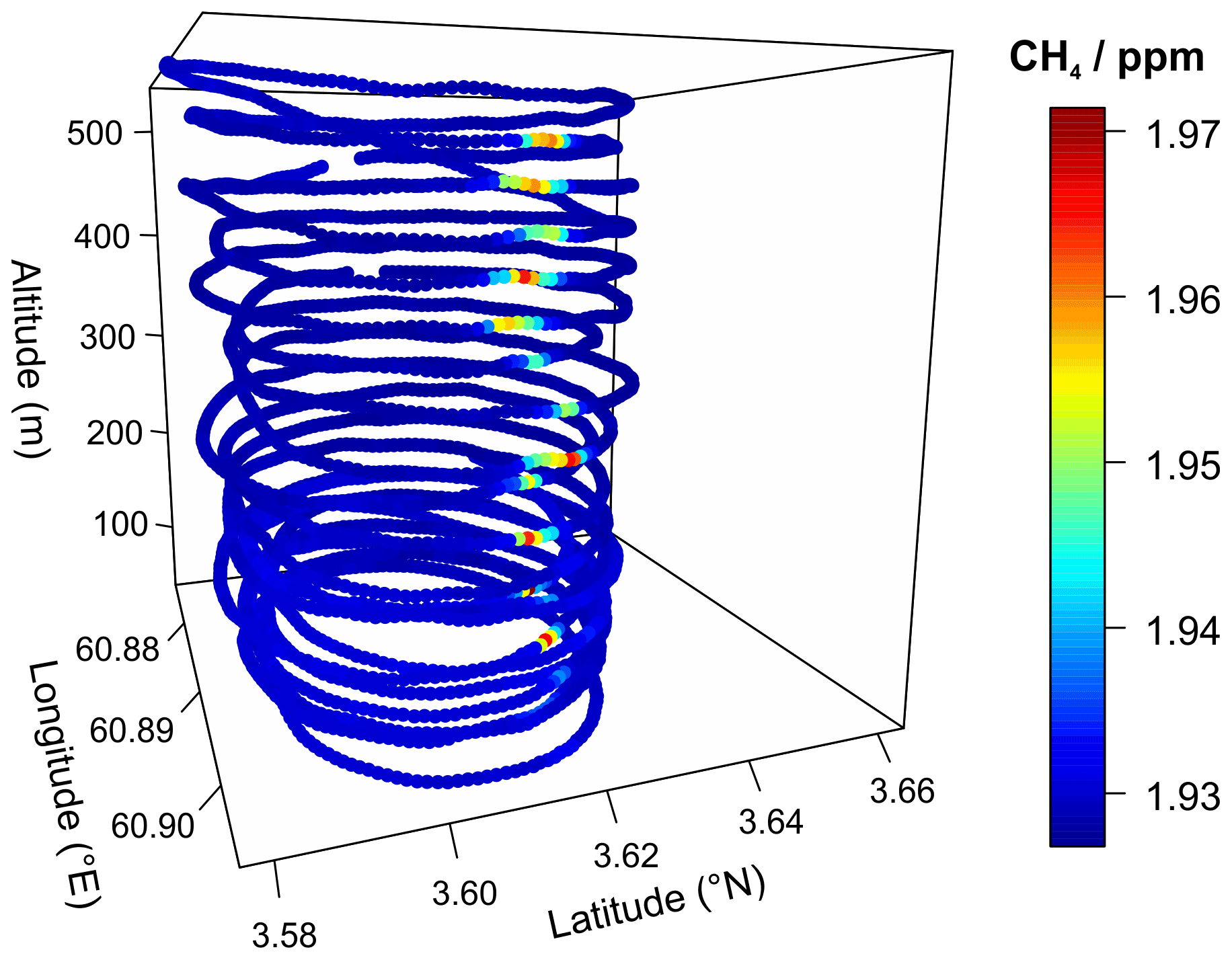
Figure B3 A 3-dimensional map of the flight pattern of the Scientific Aviation (Sci Av) aircraft sampling a CH₄ plume from an offshore O&G facility.

During all flight surveys, background concentrations were consistently invariable relative to observed downwind enhancements (see Figs. B1 and B3) by virtue of the remote maritime sampling environment and absence of significant nearby pollution sources. This aided detection of any CH₄ plumes downwind of facilities. Overall, wind fields were stable over the course of the flight surveys, facilitating the mass balance methodology described in Sect. 3.1 of the main paper. Across all FAAM and Scientific Aviation flights, wind speeds varied between 1 and 19 m s⁻¹. Observed wind directions were also consistent during the flights, with FAAM flights C191 and C197 experiencing southerly winds and flight C193 experiencing northeasterlies (as shown in Fig. S3).