the Creative Commons Attribution 4.0 License.
the Creative Commons Attribution 4.0 License.
 | 04 Apr 2022
A stratospheric prognostic ozone for seamless Earth system models: performance, impacts and future
Beatriz M. Monge-Sanz
Alessio Bozzo
Nicholas Byrne
Martyn P. Chipperfield
Michail Diamantakis
Johannes Flemming
Lesley J. Gray
Robin J. Hogan
Luke Jones
Linus Magnusson
Inna Polichtchouk
Theodore G. Shepherd
Nils Wedi
Antje Weisheimer
We have implemented a new stratospheric ozone model in the European Centre for Medium-Range Weather Forecasts (ECMWF) system and tested its performance for different timescales to assess the impact of stratospheric ozone on meteorological fields. We have used the new ozone model to provide prognostic ozone in medium-range and long-range (seasonal) experiments, showing the feasibility of this ozone scheme for a seamless numerical weather prediction (NWP) modelling approach. We find that the stratospheric ozone distribution provided by the new scheme in ECMWF forecast experiments is in very good agreement with observations, even for unusual meteorological conditions such as Arctic stratospheric sudden warmings (SSWs) and Antarctic polar vortex events like the vortex split of year 2002. To assess the impact it has on meteorological variables, we have performed experiments in which the prognostic ozone is interactive with radiation. The new scheme provides a realistic ozone field able to improve the description of the stratosphere in the ECMWF system, as we find clear reductions of biases in the stratospheric forecast temperature. The seasonality of the Southern Hemisphere polar vortex is also significantly improved when using the new ozone model. In medium-range simulations we also find improvements in high-latitude tropospheric winds during the SSW event considered in this study. In long-range simulations, the use of the new ozone model leads to an increase in the correlation of the winter North Atlantic Oscillation (NAO) index with respect to ERA-Interim and an increase in the signal-to-noise ratio over the North Atlantic sector. In our study we show that by improving the description of the stratospheric ozone in the ECMWF system, the stratosphere–troposphere coupling improves. This highlights the potential benefits of this new ozone model to exploit stratospheric sources of predictability and improve weather predictions over Europe on a range of timescales.
- Article
(19802 KB) - Full-text XML
- BibTeX
- EndNote


The new emerging generation of seamless Earth system models (ESMs) needs to be developed in ways that allow accurate performance on timescales from weather to climate, including seasonal and subseasonal timescales. This requires slow-evolving processes that influence the troposphere, like stratospheric processes, to be realistically included.
The links between stratospheric ozone, polar vortex dynamics and extreme winter weather over Europe are being increasingly recognised (e.g. Kolstad et al., 2010; Waugh et al., 2017; Kretschmer et al., 2018). Lack of detail in the description of the stratosphere is also linked to an unrealistic representation of stratosphere–troposphere coupling, which makes most existing models unable to exploit all potential sources of predictability deriving from the stratosphere (e.g. Scaife et al., 2016). The stratospheric ozone layer accounts for 90 % of the total existing atmospheric ozone and plays fundamental roles for atmospheric processes and for life on Earth. Ozone in this atmospheric region provides a vital shield against harmful ultraviolet (UV) radiation, preventing the most energetic UV-C and UV-B wavelengths (wavelength bands below 300 nm) from reaching the Earth's surface. UV radiation is absorbed by ozone in the stratosphere via very exothermic reactions. Therefore ozone is the main player in shaping the vertical temperature profile in the stratosphere and has a fundamental role in the interactions between radiation and dynamics in this region, as well as in the exchange of air masses with the troposphere. Unlike ozone in the troposphere, where its influence on physics and dynamics is dwarfed by the influence of other meteorological phenomena, a realistic distribution of ozone in the stratosphere is essential to correctly model the dynamical behaviour in this region.
Interannual dynamical variability of the polar vortex, in both hemispheres, causes large differences in the amounts of ozone depletion from year to year. In the Northern Hemisphere (NH), the occurrence of sudden stratospheric warming (SSW) events, with temperatures in the polar stratosphere experiencing very rapid increases, leads to significantly less Arctic ozone loss than during cold Arctic years without SSW disturbances (e.g. Monge-Sanz et al., 2011; Solomon et al., 2014; Strahan et al., 2016). Over Antarctica, the formation of the ozone hole every year is caused by the presence of ozone-depleting substances (ODSs) in the atmosphere, but its extent and duration depends on the particular dynamics of the polar vortex each year. The amount of ozone depletion then feeds back to temperature and winds through radiative interactions. Thus, correctly simulating the amount of polar stratospheric ozone depletion during late winter/spring and allowing it to interact with radiation has also the potential to improve the way models reproduce stratosphere–troposphere coupling.
Stratospheric ozone research has been very active during the past 30 years (World Meteorological Organization, 2019). Nowadays, the most pressing questions in this field concern the links between ozone, climate change and weather extremes. To accurately tackle them, we need tools that can seamlessly operate across different timescales, from weather to climate.
New seamless ESMs that integrate climate and weather elements of the Earth system are starting to be developed and will provide valuable tools to address such questions. How to most efficiently incorporate appropriate descriptions of stratospheric processes, including stratospheric ozone, in these ESMs is still an open question. Such descriptions will need to exhibit the right compromise between realism and computational cost to be able to adequately perform at all timescales.
The Antarctic ozone hole was first discovered in the mid-1980s, and understanding processes regulating the amount and distribution of ozone in the stratosphere became a high scientific priority for societal needs. For this reason, and to monitor the effectiveness of the Montreal Protocol, a set of complex atmospheric models was specifically developed to address stratospheric-ozone-related questions: chemistry-transport models (CTMs) and chemistry-climate models (CCMs) became the best modelling tools to understand links between chemical and dynamical factors governing the formation, distribution and destruction of stratospheric ozone. Nowadays, these modelling tools include very detailed atmospheric chemistry processes, based on the most-up-to-date scientific knowledge, and can provide very accurate simulations of stratospheric ozone (e.g. Eyring et al., 2007; Morgenstern et al., 2017).
Nevertheless, such full-chemistry level of detail is not affordable for high-resolution multiple ensemble weather forecasting simulations, because of computational costs. Alternative stratospheric descriptions that are both realistic and affordable for all timescales are key needs for emerging seamless systems. In this work we assess the feasibility and performance of a linear model for stratospheric ozone that can be implemented in any global circulation model (GCM) within an ESM at very low computational cost, yet providing quality comparable to the ozone field from world-leading full-chemistry models.
The first linear ozone model was formulated by Cariolle and Déqué (CD) (Cariolle and Déqué, 1986) when the heterogeneous chemistry of the ozone hole was still unknown, and therefore the scheme parameterised only the effects of ozone gas-phase chemistry, ignoring the heterogenous chemistry processes responsible for polar ozone loss. Subsequent versions of the CD model kept the initial approach but included an additional term to take into account the polar destruction of ozone at low temperatures (Cariolle and Teyssèdre, 2007). This is the ozone model currently used by the Integrated Forecasting System (IFS) of the European Centre for Medium-Range Weather Forecasts (ECMWF). However, this CD approach has significant limitations in the way it represents heterogeneous ozone loss.
An alternative linear model, hereafter called the BMS model, was more recently developed by Monge-Sanz et al. (2011). The BMS model, as the CD one, is a linear representation of stratospheric ozone sources and sinks as a function of ozone concentrations and temperature. But the BMS model, unlike the CD one or any other previous linear ozone model, consistently includes both gas-phase and heterogenous chemistry for stratospheric ozone. Monge-Sanz et al. (2011) tested this new ozone model within the SLIMCAT 3D chemistry-transport model (CTM) used to obtain the linear scheme, showing the superiority of the BMS scheme over the CD scheme in a multiannual run covering the period 1991–2002. In their study they showed the capacity of the new ozone scheme to provide a stratospheric ozone field of comparable quality to the ozone field from the SLIMCAT full-chemistry model. More details on the differences between the BMS and the CD ozone models are given below in Sect. 2.1, and a full discussion comparing both formulations can be found in Monge-Sanz et al. (2011).
Besides the above-mentioned decadal simulations within the SLIMCAT CTM, the BMS scheme has already been adopted by global models for different applications, from numerical weather forecasting to tropospheric air quality (Jeong et al., 2016; Badia et al., 2017), because of the more realistic simulation of stratospheric ozone it provides, compared to other available options like observation-based monthly climatologies or the CD scheme, for models that cannot afford stratospheric full-chemistry modules.
For the present study we have implemented the BMS ozone in the ECMWF general circulation model (GCM) and compared the performance of the new BMS and the default CD ozone model schemes in terms of the ozone distributions they provide. Then we have evaluated the way stratospheric ozone impacts meteorological fields at different timescales. This is the first time that the performance of an ozone model has been assessed for different timescales in a GCM, with the goal of evaluating its feasibility for seamless Earth systems simulations.
The structure of this article is as follows: Sect. 2 describes the model configuration used and the set of experiments designed for this study, as well as giving an overview of the observational datasets used for validation of our model results. Section 3 shows the ozone distribution results obtained for different experiments, regions and case studies. Then the impacts on meteorological fields are discussed in Sect. 4. The summary of results and conclusions for this study is found in Sect. 5, which also provides a discussion of future work and recommendations.
2.1 New ozone model in the IFS
We have implemented the stratospheric ozone model described by Monge-Sanz et al. (2011), the BMS ozone scheme, within the ECMWF Integrated Forecasting System (IFS).
The scheme represents the effects of stratospheric ozone sources and sinks following a linear approach, so that a CTM or GCM can simulate the time evolution of ozone by including an advected tracer for which the local concentration f (i.e. the local net ozone chemical production minus loss) evolves in time according to the following equation:
where the coefficients ci () are tendencies derived from the full-chemistry CTM runs, and the terms , and are climatological reference values (in this case obtained from the full-chemistry output fields) for the ozone concentration f, temperature T and partial column of ozone above the considered location . The coefficients ci and the climatological terms are provided as a function of latitude, pressure and month. For complete details on the calculation methodology and CTM runs leading to this ozone model, see Monge-Sanz et al. (2011). A full discussion on the differences between this new ozone model and the default CD scheme used by the ECMWF operational system can also be found in Monge-Sanz et al. (2011). For convenience, we also briefly describe here the main differences regarding, most importantly, the treatment of heterogeneous chemistry but also differences in the photochemical model runs to derive the schemes, meteorological forcing fields and resolution. For completeness, we include here below the equation of the default CD scheme. The time evolution of the ozone concentration in the default ECMWF CD scheme is based on the expression
where the tendency coefficients ci () include only gas-phase chemistry effects, making it necessary to add the fifth term and the corresponding coefficient c4 to account for ozone destruction related to heterogenous chemistry processes. ClEQ is the equivalent chlorine content of the stratosphere and varies from year to year. This fifth term is only active when temperature falls below 195 K in daytime for latitudes polewards of 45∘, and the coefficient c4 is calculated with different methods and approximations from the rest of the coefficients, reducing the consistency of the approach. Conceptually, this kind of term is too restrictive with respect to the current understanding of heterogeneous processes. For instance, in reality the temperature threshold for the formation of polar stratospheric clouds (PSCs) actually depends on altitude and trace gas concentrations (e.g. Hanson and Mauersberger, 1988; Tritscher et al., 2021). Another shortcoming in the heterogeneous approach in Eq. (2) is that it assumes chlorine activation and O3 destruction by sunlight take place at the same time. Actually, the activation of air masses takes place during the polar night inside the polar vortex, when temperature is low enough (e.g. Nakajima et al., 2016). Later, when spring sunlight returns to polar latitudes, the processed air is able to destroy ozone. However, the destruction can also happen during winter if activated air masses reach lower latitudes (e.g. by filamentation or vortex break-up) and are exposed to sunlight. This latter kind of process is completely missed by a localised simple temperature threshold term like the one in the default ECMWF scheme.
The treatment of heterogeneous chemistry is one fundamental difference in the new (BMS) scheme, which includes stratospheric ozone chemistry processes, both gas-phase and heterogeneous chemistry, in a consistent embedded way for all locations using only the first four linear coefficients ci (). Unlike previous stratospheric ozone linear schemes, the BMS scheme is the first one to include heterogeneous chemistry effects and gas-phase chemistry in a consistent, implicit way in all terms of Eq. (1). Since the BMS scheme coefficients are obtained taking into account all heterogenous chemistry included by the CTM, heterogeneous chemistry is embedded in all the terms in Eq. (1) and not restricted to limited regions and times as in the CD scheme. This new approach was shown to be very beneficial for the representation of ozone at high latitudes (Monge-Sanz et al., 2011).
In addition, the coefficients for the new scheme have been derived from a 3D full-chemistry model, in contrast to the default ozone scheme used by ECMWF, which is based on a 2D photochemical model. This provides additional information on spatial variability of the chemical tendencies represented by the coefficients. To derive the chemical tendencies, the box model used to derive the coefficients for the BMS scheme was initialised from a 3D SLIMCAT full-chemistry reference run forced by ERA-40 meteorological fields, corresponding to year 2000, while the 2D model used to derive the CD coefficients was run from output from the climate model ARPEGE (Action de Recherche Petite Echelle Grande Echelle) averaged for the period 1990–2000 (Cariolle and Teyssèdre, 2007). Deriving coefficients from one representative meteorological year does not limit the performance of the BMS model. Monge-Sanz et al. (2011) compared two versions of the scheme, one was based on a representative year with cold winter conditions (year 2000), and another version was based on a year with mild winter conditions (year 2004). Their results demonstrated that when the coefficients are derived from years with more extreme conditions (cold winters), the scheme is able to realistically capture ozone distributions for both cold and mild conditions.
Regarding vertical resolution of the schemes, the CD scheme original number of levels is larger (60 levels) than that of the original BMS number of levels (24 levels). Both schemes are then interpolated to the same grid for each experiment in the ECMWF model, using the same interpolation method for both to ensure numerical consistency.
Despite the relatively coarse vertical resolution, as Monge-Sanz et al. (2011) discussed, the new approach allows for more realistic interactions between parameterised ozone, radiation and temperature, and therefore better response and feedbacks to meteorological conditions, than previous ozone parameterisation approaches.
2.2 ECMWF model experiments
We have used the Integrated Forecasting System (IFS) of ECMWF to run forecast experiments at medium-range (10 d, where d stands for day) and long-range (seasonal) timescales. The IFS configuration in each pair of experiments (control and new) differs only in the scheme used to model stratospheric ozone and whether prognostic ozone is used or not by the radiation scheme. All other aspects of the model configuration remain identical.
2.2.1 Medium-range experiments
A list of medium-range forecast experiments, corresponding periods and model configurations is shown in Table 1. All model experiments, unless otherwise stated, are 10 d forecast runs using the 41r1 cycle version of the IFS, which was operational between May 2015 and March 2016. For the medium-range experiments, the model has been run at spectral resolutions of T511 and T159, with 91 vertical levels up to 0.01 hPa. Both schemes are interpolated from their original resolutions onto the same IFS grid for each experiment, using the same interpolation method for both schemes. First, linear interpolation in pressure is performed followed by linear interpolation in latitude. We apply this for the different vertical level configurations in IFS; this is the usual practice at ECMWF for all parameterisations that are sensitive to the vertical discretisation.
Table 1Medium-range (10 d forecasts) IFS model experiments using the default IFS Cariolle v2.9 ozone scheme (CD), or the new BMS ozone scheme (BMS). For each experiment information on model version, resolution, period covered and whether prognostic ozone was interactive with radiation is also included.
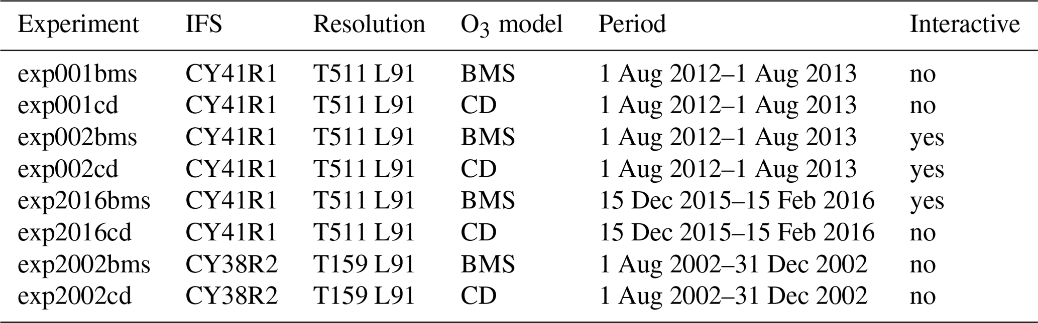
Ozone concentrations are initialised from operational analyses at the start of each experiment (00:00 UTC on day 1), and then, unless otherwise stated, ozone is left to evolve freely along the duration of the experiment using either the CD or the BMS scheme; 1-month initial spin-up is allowed for the experiments.
In the default IFS configuration the radiation scheme does not employ the prognostic ozone; instead it uses an ozone climatology in the form of zonal-mean monthly-mean ozone values. In the IFS version used in this study, the ozone climatology is derived from the MACC reanalysis (Inness et al., 2013), a dataset that covers the period 2003–2011 at T255 horizontal resolution on 60 vertical levels. However, for some of our experiments the standard IFS model has been adapted so that the prognostic ozone provides the input to the radiation scheme (Table 1), thus allowing for feedbacks between the ozone scheme and model dynamics.
2.2.2 Long-range experiments
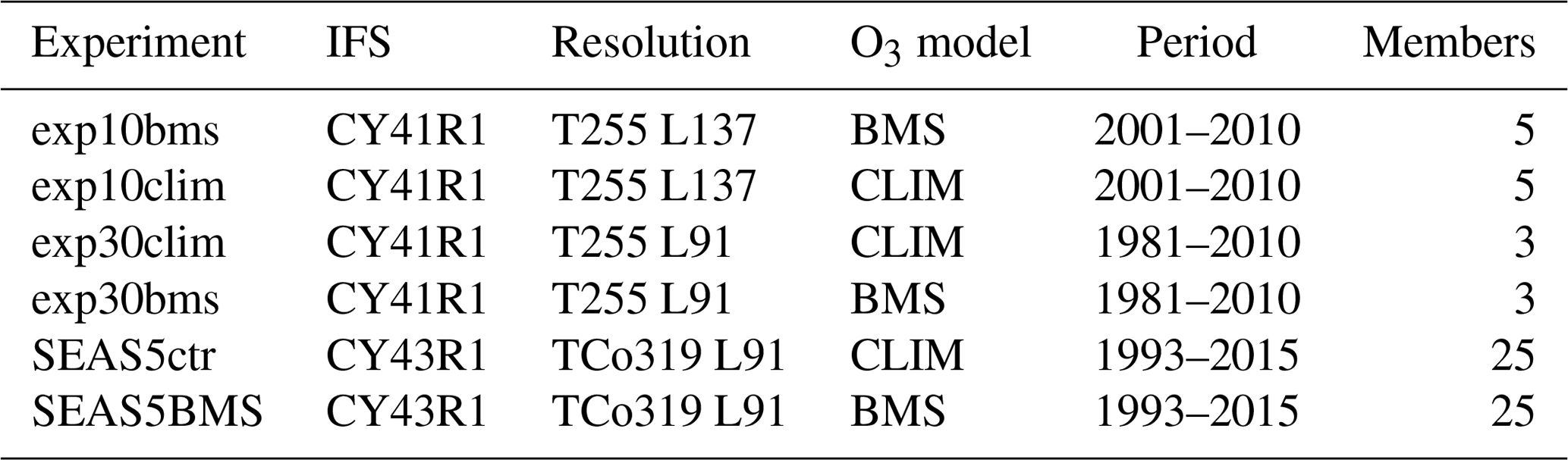
Table 2 provides an overview of the long-range seasonal experiments we have performed for this study. We have performed two five-member seasonal experiments, with May and November start dates and a 7-month integration range, for the period 2001–2010. One of these experiments is using the default ozone configuration (CD scheme and no feedback onto radiation), and the other one is using the new BMS scheme interactive with radiation, both experiments with a T255 resolution and 137 vertical levels up to 0.01 hPa. Initialisation data for these experiments come from ERA-Interim reanalysis fields (Dee et al., 2011). These two long-range experiments were performed with an experimental version of 41r1 that included research developments towards the new ECMWF seasonal forecasting System 5; the BMS stratospheric ozone model is one of such developments (Knight et al., 2016; Johnson et al., 2019). Another set of two seasonal experiments with the two ozone configurations has additionally been performed using the 41r1 coupled version of IFS operational in 2016, with horizontal resolution T255 and 91 vertical levels, May and November start dates, and a 7-month integration range. These are three-member ensemble experiments covering the 30-year period 1981–2010, to be able to compare results with the ERA-Interim reanalysis dataset.
2.3 Datasets for validation
In situ observations from the global network of ozone sondes have been used for the validation of the modelled ozone vertical profiles. These observations come from the networks of the World Ozone and Ultraviolet Radiation Data Centre (WOUDC, https://woudc.org/data/explore.php, last access: 21 February 2022), the Network for the Detection of Atmospheric Composition Change (NDACC), the Norwegian Institute for Air Research (NILU), the Southern Hemisphere Additional Ozonesondes (SHADOZ, e.g. Thompson et al., 2017), and the National Oceanic and Atmospheric Administration (NOAA). Additional measurements from the Coordinated Airborne Studies in the Tropics (CAST) and measurements from the Match campaigns for stratospheric ozone (Harris et al., 2017; Schulz et al., 2001) have also been used. These ozone sonde observations provide a completely independent validation dataset as they are not assimilated by the (re)analyses used to provide the initial conditions in our model experiments. Ozone observations from these ozone sondes are highly reliable (±5 %) up to altitudes of 10.0–5.0 hPa.
The global reanalysis produced by the Copernicus Atmosphere Monitoring Service (CAMS), CAMSiRA (Flemming et al., 2017) has provided additional comparisons for the ozone field in our model experiments. The ERA-Interim reanalysis (Dee et al., 2011) has been used to validate meteorological fields from our experiments.
The distribution of stratospheric ozone and its time evolution for the experiments described above are shown in this section for different latitudinal regions, atmospheric events and timescales. The impact of the new ozone scheme on meteorological fields at the different timescales will be discussed in Sect. 4.
3.1 Antarctic ozone hole
Figure 1 shows the time series of monthly averaged vertical profiles of ozone, for the period August 2012–February 2013, from two experiments in which the ozone field is freely evolving along the 1-year period, but meteorology is initialised every 10 d (i.e. medium-range 10 d meteorological forecasts). One of the experiments uses the new BMS ozone (exp001bms); the other uses the default CD ozone scheme (exp001cd). By comparing ozone concentrations from these experiments with ozone sonde measurements (Fig. 1, left panel), we can clearly see the improvement obtained with the new ozone scheme over the Antarctic region, both in terms of vertical distribution of ozone concentrations and in terms of time evolution of the concentrations, especially during and after the ozone hole season. The recovery of the ozone concentrations after October is also much more realistic with the new ozone model.

Figure 1Monthly averaged time series of the vertical profiles of ozone (mPa) over southern high latitudes (55–90∘ S) for the period August 2012–August 2013. Panels show ozone concentrations as measured by ozone sondes (a), as simulated with the new ozone scheme in IFS (b) and as simulated with the default IFS scheme (c). The vertical distribution and the time evolution of the ozone hole and its recovery are better represented by the new scheme.
The distribution of differences between these model runs and the sonde observations (model − observations) are shown in Fig. 2. The largest differences for the BMS model run (up to 3 mPa) are found in August between 100–200 hPa and in September–October between 20–50 hPa; for all other months and regions differences are smaller (within ±1.5 mPa). However, for the CD model run positive biases (of up to 4 mPa) between 100–200 hPa persist over the first 6 months, and differences with observations are larger between 30–100 hPa from September–April (negatively biased, with differences values of up to −5 mPa).
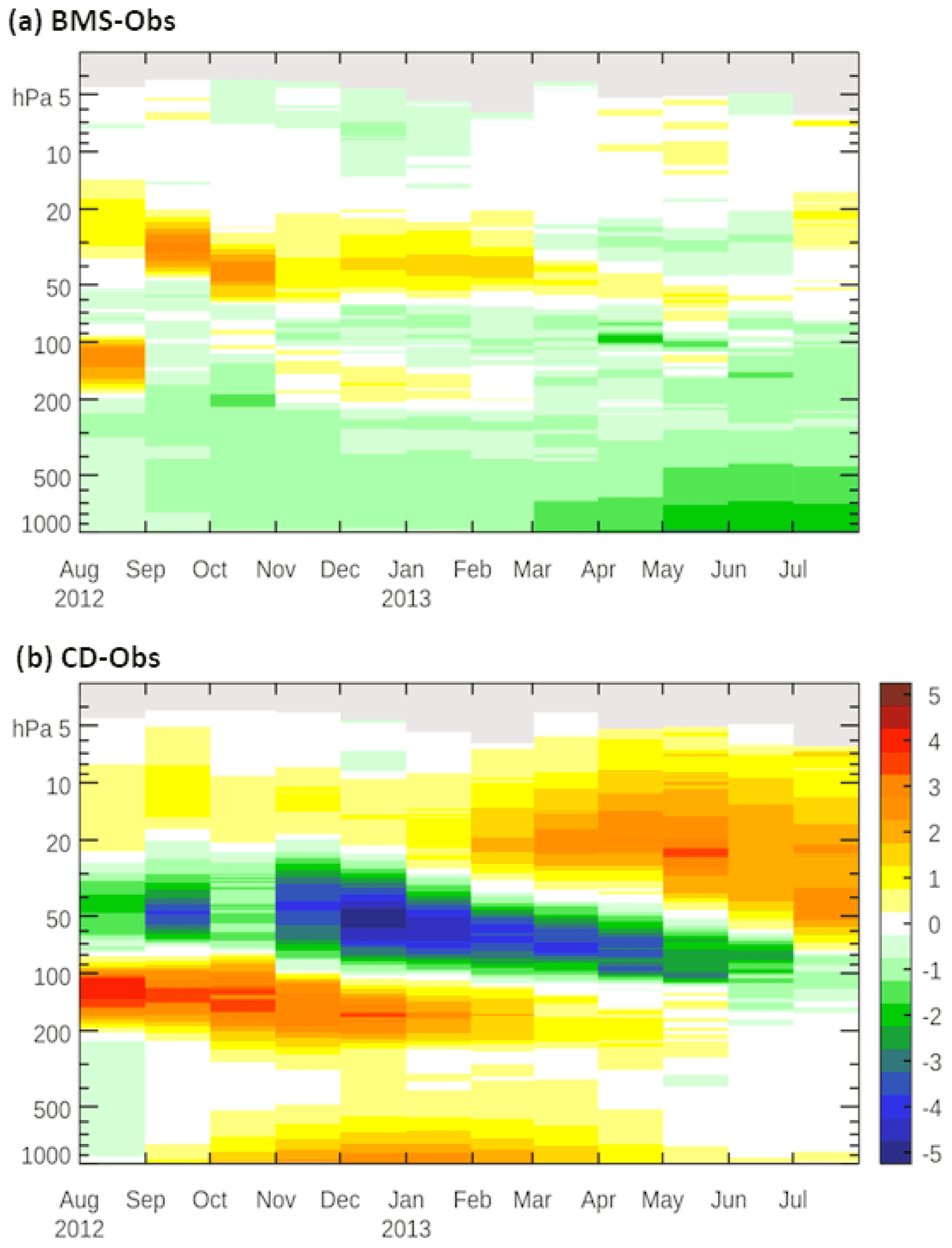
Figure 2Differences (mPa) with respect to ozone sonde observations for the monthly averaged ozone vertical profiles shown in Fig. 1; differences shown (model − observations) are for (a) the model experiment using the BMS ozone scheme and (b) the model experiment using the default CD scheme.
The better performance of the new BMS scheme is mainly due to the new formulation of the heterogeneous chemistry treatment, which has been derived from realistic full chemistry at all altitudes, unlike the fifth term in Eq. (2) that is representative of an altitude of approximately 20 km. Moreover, the default scheme specifies a dependence on the square of the chlorine content (ClEQ)2 which is not representative of typical atmospheric conditions in the activated polar vortex (e.g. Searle et al., 1998). In the CD model run differences centred around 20 hPa are also larger than in the BMS run for March–July months.
3.1.1 Antarctic vortex split 2002
In 2002 a vortex split was observed for the first time over the Antarctic region, following a stratospheric major warming in the winter stratosphere (e.g. Krüger et al., 2005; Roscoe et al., 2005). Such events are relatively common over the Arctic, where a sudden stratospheric warming can take place in almost half of winters (e.g. Butler et al., 2017).
The unusual Antarctic event in 2002 had an enormous impact on the evolution of the ozone hole, which was one of the smallest ones ever recorded. The atypical characteristics of this 2002 vortex split are a challenging benchmark to evaluate the adaptability of the new ozone scheme to meteorological and chemical conditions that very significantly differ from climatological conditions in this region.
Figure 3 shows the time evolution of the O3 vertical distribution at two Antarctic radiosonde stations, Syowa (69∘ S, 40∘ E) and the South Pole (90∘ S). Results are from 10 d forecast experiments in which the ozone field is left to evolve freely along the whole length of the experiment (1 August 2002–1 January 2003); the experiments we compare here are exp2002bms and exp2002cd from Table 1.
After the vortex split at the end of September, the ozone destruction over the station of Syowa stopped and ozone concentrations quickly recovered; this is well captured by the new scheme but not by the default scheme, which shows too low maximum concentrations compared to observations for October–December. Over the South Pole station in October both model schemes simulate larger concentrations than observed, but in November–December it is again the new scheme that simulates a more realistic recovery of ozone values. Differences between these model runs and observations exhibit similar structure and values to those in Fig. 2 (figure not shown).

Figure 3Monthly averaged time series of vertical profiles of ozone (mPa) over the Southern Hemisphere stations of Syowa (69∘ S, 40∘ E) (a–c) and the South Pole (90∘ S) (d–f). Period shown is August–December 2002, corresponding to the first Antarctic vortex split and ozone hole recovery afterwards.
The more realistic link with temperature in the new scheme, for gas-phase and heterogenous chemistry, makes it capable to respond to the rapid changes in atmospheric dynamics that take place in an event like the 2002 Antarctic vortex split; Monge-Sanz et al. (2011) showed that this kind of response resembles that of a full-chemistry 3D global model. In the default scheme, the artificially detached heterogenous term cannot adapt in the same way.
3.1.2 Interannual variability of the ozone hole season
For seasonal timescales, here we analyse two of the experiments described in Sect. 2.2.2 (exp10bms and exp10clim in Table 2) covering the period 2001–2010. Figure 4 shows the time evolution of the stratospheric ozone hole area and depth for these two model experiments, as well as for the CAMSiRA reanalysis ozone field for the overlapping years (2003–2010). To quantify the intensity and extent of the ozone hole, Fig. 4 displays the total ozone column (TOC) minimum value and the ozone hole size fraction (area with TOC values below 220 DU for latitudes south of 62∘ S) from July to December.
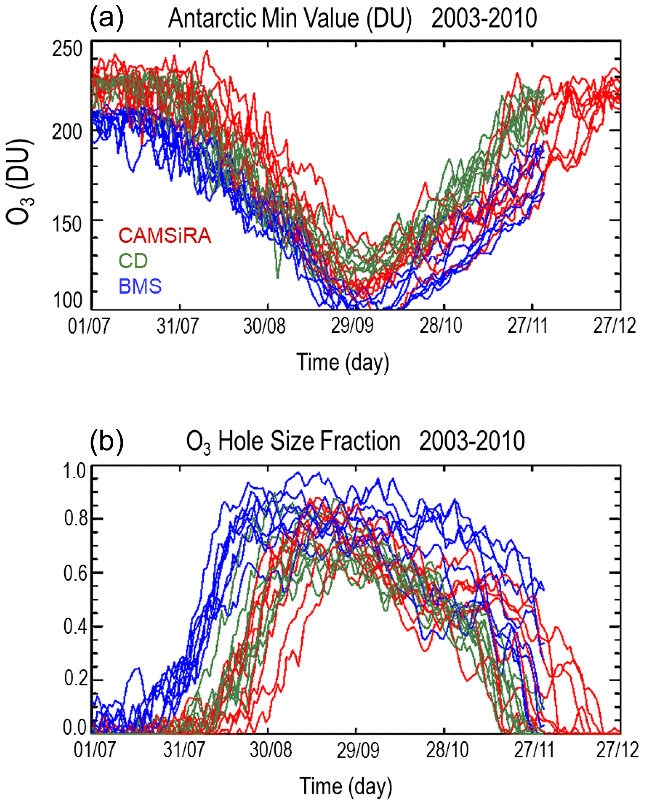
Figure 4Time series of daily values of the total ozone column (DU) over the Antarctic region (a) and of the ozone hole size fraction (b) from July to December, for the years 2003–2010. Model results come from long-range model ensemble experiments with May starting date (see text for details) using the default stratospheric ozone scheme (green lines) and the new stratospheric ozone scheme (blue lines). The values corresponding to the CAMSiRA reanalyses are also shown (red lines).
Table 2Seasonal experiments using the new ozone scheme (BMS) or the default ozone configuration in which the radiation sees an ozone climatology (CLIM). For each experiment information on model version, resolution, period covered and the number of ensemble members is also included.
Both model experiments capture the formation and evolution of the ozone hole, but the new ozone scheme produces more ozone loss, and over a larger area, than that reproduced by the CAMSiRA reanalyses. Total ozone column values from CAMSiRA are known to be too large (by up to 20 DU) over the Antarctic region during July–September months when compared to independent observations for the period considered here (Fig. 16 in Flemming et al., 2017). The new BMS scheme for the July–September months is showing lower minimum values than CAMSiRA, 18 DU lower on average (upper panel in Fig. 4), implying more realistic ozone column values. For later months in the year, Fig. 16 in Flemming et al. (2017) shows smaller biases for CAMSiRA, mainly positive during October and mainly negative afterwards. For these later months of the year our results with the BMS scheme show overall agreement with the reanalysis, with minimum Antarctic values within the CAMSiRA range. This, together with the results we have shown above in Sect. 3.1, adds confidence to the ozone hole structure obtained with the new BMS scheme in these seasonal experiments.
Interannual variability is more realistic with the new BMS scheme compared to the reanalysis, while the default scheme does not show enough variability, especially for the fraction area covered by the ozone hole, which indicates that the description of heterogenous chemistry processes in the default scheme is not realistic enough to deal with meteorological interannual variability in the Antarctic region. Since CAMSiRA uses the CD scheme in the stratosphere, Fig. 4 also suggests that with the new BMS scheme, assimilation increments in the reanalysis would be reduced for the ozone field.
The formation of the ozone hole commences earlier when using the new ozone scheme. This is at least partly due to the fact that the new ozone scheme is able to capture the ozone loss that in late winter starts to occur at the edge of the polar vortex, while the heterogeneous treatment in the scheme currently used by ECMWF cannot reproduce this process. The ozone hole closure shows large interannual variability in the reanalysis, and the simulation with the new ozone scheme is in better agreement regarding this interannual variability. The model experiments shown in Fig. 4, both with the CD scheme and the BMS scheme, end on 30 November, and closure dates beyond this date cannot be analysed. However, from the lower panel in Fig. 4, we can see that the default CD scheme does not show enough variability in ozone hole closure compared to reanalysis data, while the BMS scheme exhibits variability in better agreement with the reanalysis.
For those years with an early closure, the overall duration of the ozone hole is similar with the new scheme and in the reanalysis, but the timing of the ozone hole formation occurs earlier in the new ozone model run than in the reanalysis. In contrast, the duration and extent of the ozone hole with the default ozone scheme is reduced compared to both the reanalysis and the new scheme.
It is also worth noting that these ozone hole diagnostics are related to the total ozone column (TOC) and that realistic TOC values do not necessarily imply that the depletion in the model is occurring at the right altitudes. For similar TOC values over the Antarctic, we have shown that the new BMS scheme provides a much more realistic ozone vertical profile than the default ozone scheme in the ECMWF model (Sect. 3.1), also in agreement with previous studies using the BMS scheme (Monge-Sanz et al., 2011; Jeong et al., 2016; Badia et al., 2017).
Regarding the duration and extent of the ozone hole, several studies have shown how the Antarctic stratospheric ozone hole feeds back to dynamics and radiation causing changes in tropospheric winds and climate (e.g. Kang et al., 2011; Polvani et al., 2011; Orr et al., 2012; Haase et al., 2020). It is therefore important that future Earth system models use a stratospheric ozone description that realistically captures the ozone hole intensity and evolution to correctly simulate tropospheric trends.
3.2 Tropics and midlatitudes
3.2.1 Tropics
Over the tropics both schemes provide realistic ozone distributions in our model runs, although the maximum values are underestimated by both linear schemes compared to ozonesondes (figure not shown). This negative bias over the tropics was already documented by Monge-Sanz et al. (2011); their study showed that the upper limit imposed by the ozone climatology term in Eq. (1) means that a linear scheme of these characteristics cannot provide higher concentrations over this region than the values provided by this reference climatology term, which in the case of biases being present in this term of Eq. (1) is a caveat for these linear ozone schemes over certain regions.
Monge-Sanz et al. (2011) showed that a different choice of ozone climatology term can improve this tropical bias, although caution must be taken in selecting the climatology to ensure that performance over other regions is not degraded. This showed that the use of a carefully chosen climatology term, either from an updated run of the parent full-chemistry CTM or from a recent observation-based climatology, can improve this bias over the tropics. Although the use of an observation-based reference term is a reasonable option to improve known biases of the ozone scheme in some regions, one needs to be careful to avoid degrading the scheme’s performance in other regions and to keep internal consistency of the scheme as much as possible (see additional discussion on this point in Sect. 5.2).
3.2.2 Midlatitudes
One of the longest ozone records in Europe corresponds to the Alpine station of Hohenpeissenberg (Fig. 5). At this midlatitude location (47∘ N, 11∘ E) the two linear ozone schemes capture well the overall annual cycle (low ozone concentrations in autumn–winter and high ozone concentrations in spring–summer). However, both schemes behave differently in terms of biases. From the integrated profiles and the corresponding biases compared to observations (low panels in Fig. 5), we can see that the new scheme produces ozone column values in close agreement with observations from August to December 2012 and then underestimates column values (up to −0.7 mPa) from January to July 2013; the default ozone scheme however overestimates column values all along the year by up to 1.0 mPa.
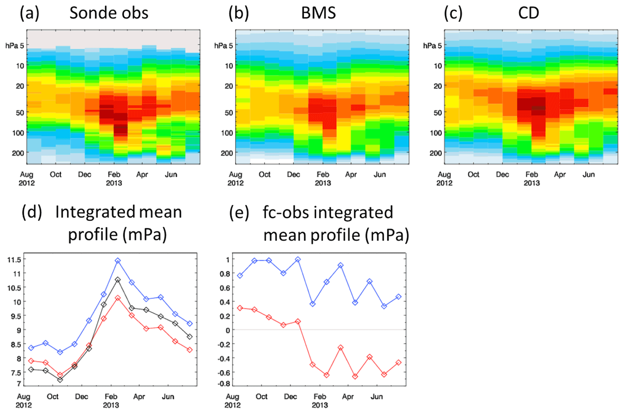
Figure 5Monthly averaged time series of the vertical stratospheric profiles of ozone (mPa), for the period August 2012–July 2013, over the European Alpine Hohenpeissenberg station (47∘ N, 11∘ E), from the observed profiles (a), the model experiment with the new ozone scheme (b), and a model experiment using the default ozone (c). The values for the integrated mean vertical profiles are shown in panel (d) for observations (black), model experiment using default option for ozone (blue) and model experiment using the new ozone scheme (red). Panel (e) shows the corresponding differences in the integrated mean vertical profile between the two forecast (fc) runs and the observations (obs), for the experiment using default option for ozone (blue) and the experiment using the new ozone scheme (red).
This overall behaviour is representative of most European midlatitude stations (figure not shown). The overestimation with the default ozone may partly be caused by ozone concentrations at high latitudes being larger and then air richer in ozone being transported towards midlatitudes.
3.3 Arctic ozone
Ozone loss in the Arctic region does not usually reach the levels found in the Antarctic. However, ozone depletion over the Arctic presents high interannual variability because of the large variations in this region's winter dynamics. Arctic winter temperature variations and vortex variability affect the formation of polar stratospheric clouds (PSCs), and thus the chemical processing that leads to ozone destruction can be largely different from year to year (e.g. Tritscher et al., 2021).
The occurrence of sudden stratospheric warming (SSW) events, with temperatures in the polar stratosphere experiencing very rapid increases, leads to significantly lower Arctic ozone loss than during cold Arctic years without vortex disturbances (e.g. Monge-Sanz et al., 2011; Strahan et al., 2016).
Ozone loss in the Arctic region is largely dependent on the number of consecutive cold days during winter and therefore on dynamics and the occurrence of SSWs. The Arctic winter 2015/16 saw anomalous polar vortex behaviour. Polar stratospheric vortex winds were stronger than usual since early winter, and then in mid-winter a minor SSW took place, followed by a major warming in late winter (e.g. Manney and Lawrence, 2016). During the minor warming in February 2016, PSCs were seen over northern England mid-latitude locations; the closest ozonesonde station is the Irish station of Valentia (52∘ N, 10∘ W).
To take into account feedbacks between ozone and dynamics during this event we ran two experiments: one with the new BMS ozone scheme interactive with radiation and one using the default ozone configuration in which the radiation sees a climatological ozone field. Monthly averaged profiles of differences (model − observations) at Valentia station in January and February 2016 show that both experiments underestimate the maximum of the ozone profile, but differences between forecast ozone and observations are smaller when using the new BMS ozone scheme interactive with radiation than using the default ozone configuration, at all pressure levels except around 150 hPa (Fig. 6).
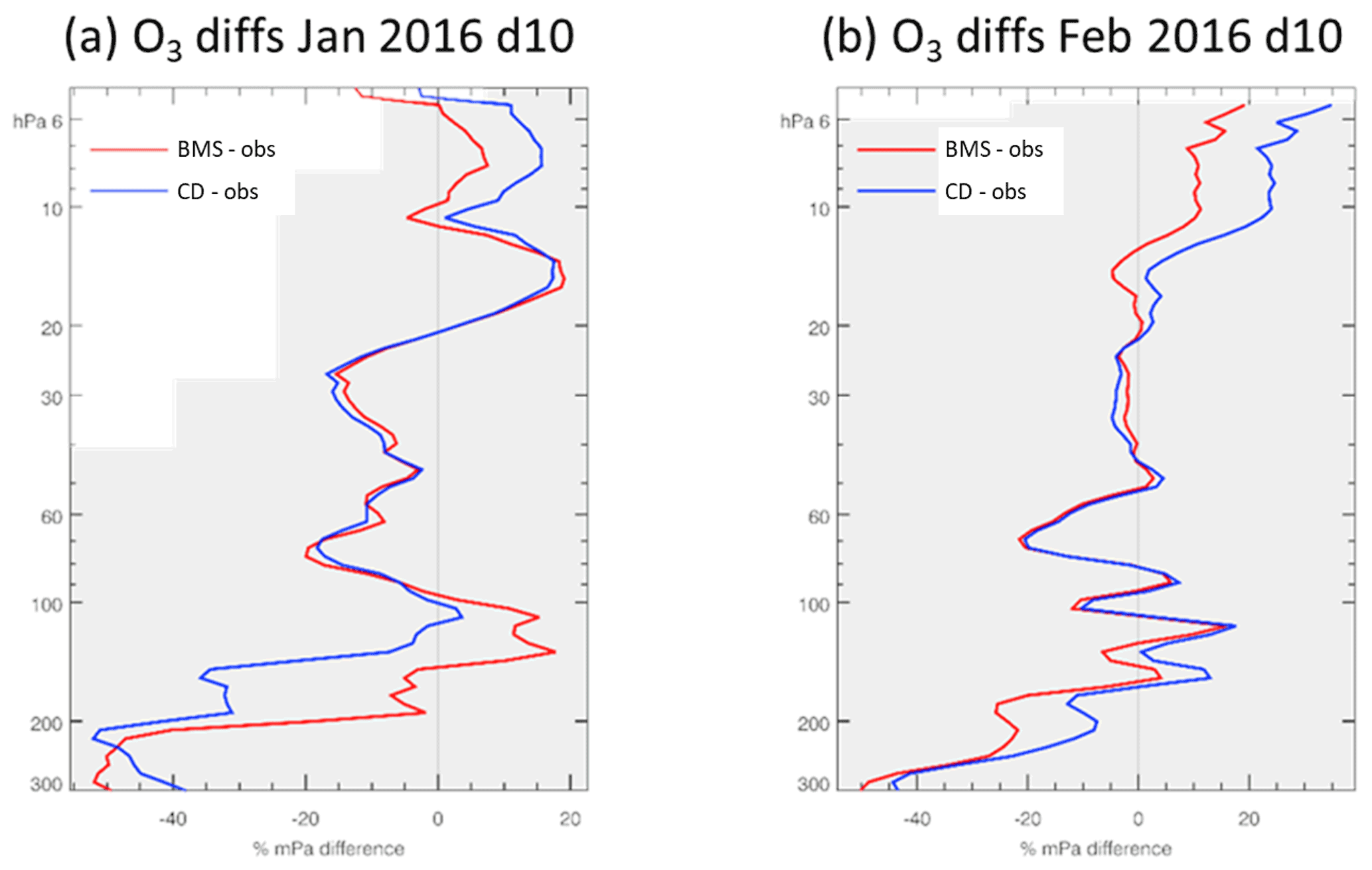
Figure 6Averaged vertical profiles of ozone percentage differences for the Irish station of Valentia (52∘ N, 10∘ W) in (a) January and (b) February 2016 for the model run using the new ozone scheme interactive with radiation (red) and the default ozone configuration (blue). Profiles used, both for model runs and observations, correspond to day 10 in the forecast runs. Shaded areas indicate the density of observation profiles for the corresponding altitude range for the considered period.
Similar differences are also seen for Arctic stations. Arctic ozone profiles corresponding to day 10 in the forecast runs are shown in Fig. 7 together with the corresponding ozonesonde observations for February 2016. Although both model runs overestimate the concentration values, and underestimate the altitude, of the ozone maximum compared to the ozonesonde profiles, the model run with the new BMS scheme results in concentrations closer to observations; the percentage differences (forecast − observed) are up to 10 % smaller with the new ozone, except at 250 hPa.
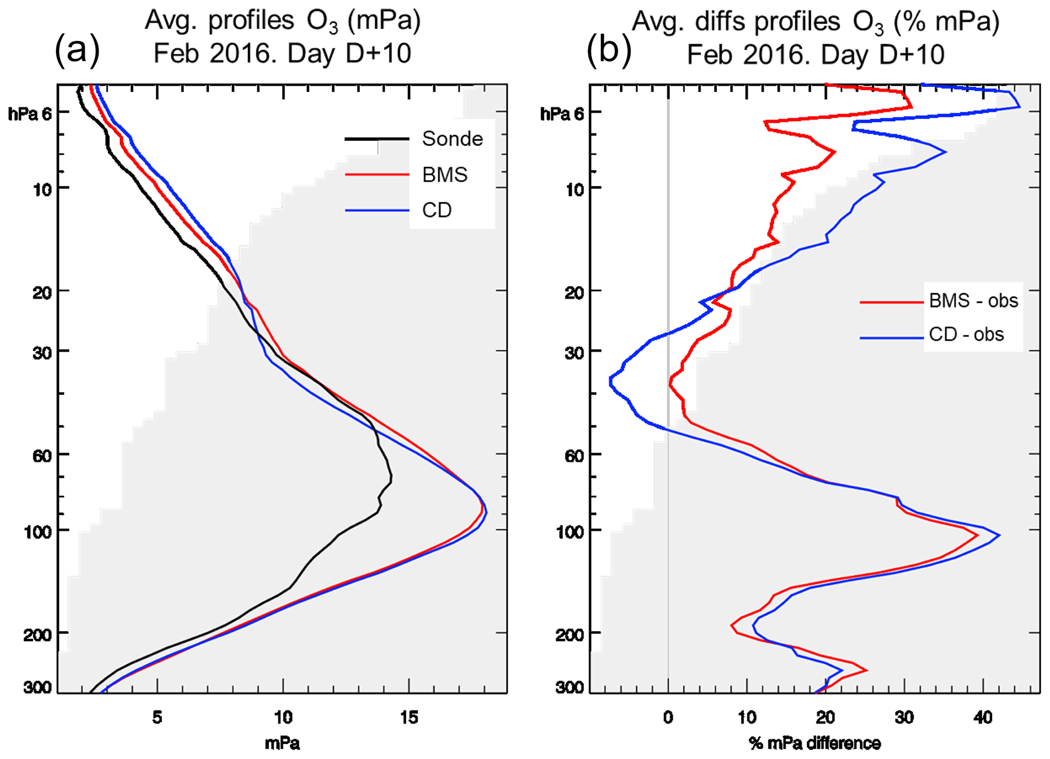
Figure 7Averaged vertical profiles of ozone (mPa) over the Arctic region in February 2016 (a) from ozonesonde observations (black), from a model run using the new BMS ozone scheme (red) and a model run using the default ozone configuration (blue). The model profiles are for day 10 in the forecast run. The percentage differences in ozone concentrations between the forecast runs and the observations are also shown (b). Shaded areas indicate the density of observation profiles for the corresponding altitude range for the considered period.
SSW events like this one in winter 2015/16 are good case studies to assess the new stratospheric ozone scheme. Important feedbacks between ozone and dynamics take place in this type of events: the occurrence of a SSW reduces the amount of ozone loss over the Arctic; therefore, more ozone is available to absorb UV radiation, which contributes to a further increase of temperature in the region.
Past versions of the operational ECMWF forecast model reproduced SSW events overall weaker (colder) than observed (e.g. Manney et al., 2008; Diamantakis, 2014); although not the only factor, this is consistent with the fact that by using an ozone climatology in the radiation scheme, past model versions could not fully reproduce the feedbacks between stratospheric ozone and rapid temperature increases that take place during SSWs. A realistic scheme for prognostic stratospheric ozone is therefore able to contribute to a better reproduction of SSW events and their feedbacks within the model.
The previous sections have shown the improved stratospheric ozone distribution and variability obtained when using the new BMS ozone model in the ECMWF system. From a weather and climate modelling perspective, we are interested in how the new representation of stratospheric ozone affects meteorological fields. To evaluate this, the prognostic ozone scheme has been made interactive with the radiation scheme in the ECMWF model. The corresponding impact on meteorological variables has been compared with results from the default ECMWF ozone configuration in which the radiation scheme uses an ozone climatology.
4.1 Impacts on medium-range forecasts
The mean error in the temperature field is shown in Fig. 8 for two forecast model experiments in which the prognostic ozone has been made interactive with the radiation scheme. Both experiments are 10 d forecast covering the period August 2012–July 2013. The only difference between the configuration of the two experiments is in the prognostic ozone model: one of them uses the CD ozone, and the other one uses the new BMS ozone. In the stratosphere (above 100 hPa), the new ozone clearly reduces the model temperature bias by up to 1 K. Smaller improvements can also be seen for lower levels in the extratropics (Fig. 8). The tropical region at 100 hPa is the only region in which the use of the new ozone scheme increases the temperature mean error. This is most probably attributable to the negative bias in tropical ozone exhibited by the BMS scheme. Although the negative ozone bias is found above 100 hPa, it means that more UV can reach lower altitudes (less ozone above), therefore less ozone below (more dissociation by UV); and with less ozone there is also a decrease in local temperature, leading to the larger negative temperature bias over the tropics at 100 hPa shown in Fig. 8. For tropospheric levels there is an overall improvement in the temperature mean error, although not everywhere for all lead times, but results for the troposphere are not statistically significant.
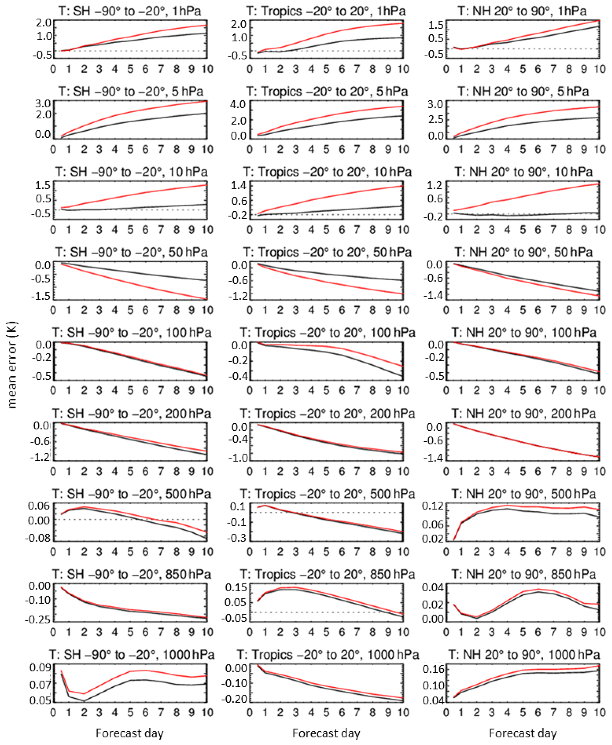
Figure 8Mean error in the temperature field (K) compared to the operational ECMWF analyses, as a function of lead time for the forecast experiment using the new BMS ozone (black) and the one using the CD ozone (red), both with prognostic ozone interactive with radiation. The two model runs consist of 10 d forecasts covering a 1-year period, from August 2012 to July 2013. The figure shows three latitudinal bands, 90–20∘ S (left column), 20∘ S–20∘ N (centre column) and 20–90∘ N (right column), for different pressure levels as labelled for each row, from 1.0 to 1000 hPa.
To display the statistical significance of these results, the differences in normalised error change in the temperature field, and corresponding significance 95 % bars, are shown in Fig. 9. The improvement in the model error in the stratosphere above 100 hPa is clearly evident and statistically significant with the new ozone. For altitudes below 100 hPa, it shows small increases in model error with the new scheme, but these are not statistically significant, except in the tropical upper troposphere and lower stratosphere (UTLS). Interpreting results in the tropical UTLS is not straightforward due to the many interplaying factors in this region, but the negative concentration bias exhibited at higher altitudes over the tropics is most probably playing a role.
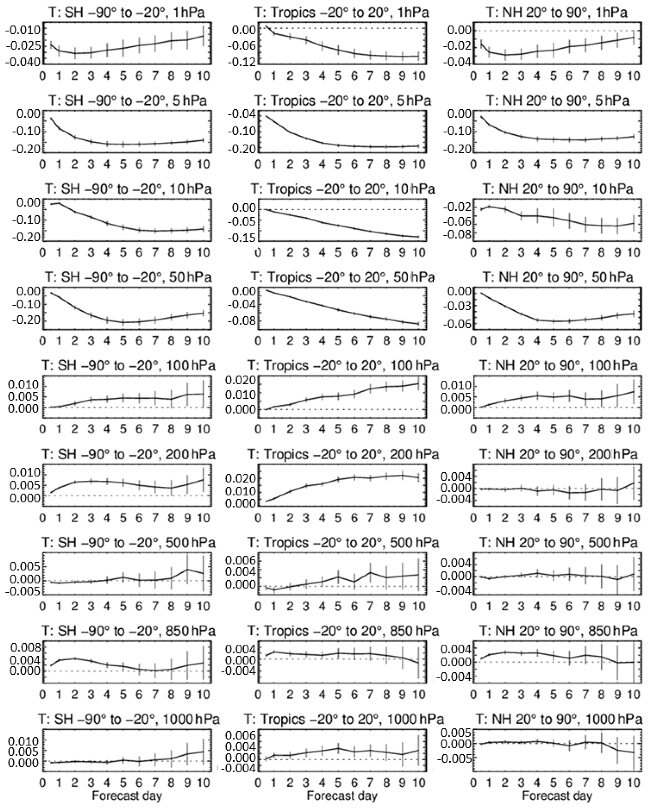
Figure 9Normalised differences in root mean square error (DRMSE) in the forecast temperature field (K) with the new and default ozone schemes, as a function of lead time. The forecast model runs cover a 1-year period, with 10 d forecasts from August 2012 to July 2013. The figure shows three latitudinal bands, 90–20∘ S (left column), 20∘ S–20∘ N (centre column) and 20–90∘ N (right column), for different pressure levels as labelled for each row, from 1.0 to 1000 hPa.
In summary, the new scheme, therefore, improves the temperature behaviour in the stratosphere without degrading the temperature field in the troposphere; the only atmospheric region where there is some degradation in the temperature field is the tropical LS, and this is at least partly due to a known bias in the new ozone scheme.
A similar comparison can be performed between the forecast experiment using the prognostic BMS ozone interactive with radiation and the default ECMWF operational configuration in which the radiation scheme uses an ozone climatology. Figure 10 shows the mean error in temperature for these two experiments, and Fig. 11 shows the corresponding differences in normalised error change with the 95 % significance bars. These results show a similar pattern to those from the comparison of the two prognostic schemes; i.e. the BMS scheme provides an improved temperature field in the stratosphere compared to the default climatology, with the exception of the tropical region at 50 hPa and the NH extratropics at the same 50 hPa level. The new ozone also provides mean error improvements for the troposphere outside the tropics, although results are only marginally statistically significant or not significant. Note also that differences in the troposphere are 1 order of magnitude smaller than in the stratosphere. In the tropical troposphere a small degradation can be found, which unlike in the comparison of both schemes now becomes statistically significant. This is related to the fact that ozone linear models are not designed for tropospheric use, and in the troposphere the use of a realistic climatology could be considered a good alternative for numerical weather prediction (NWP) purposes.
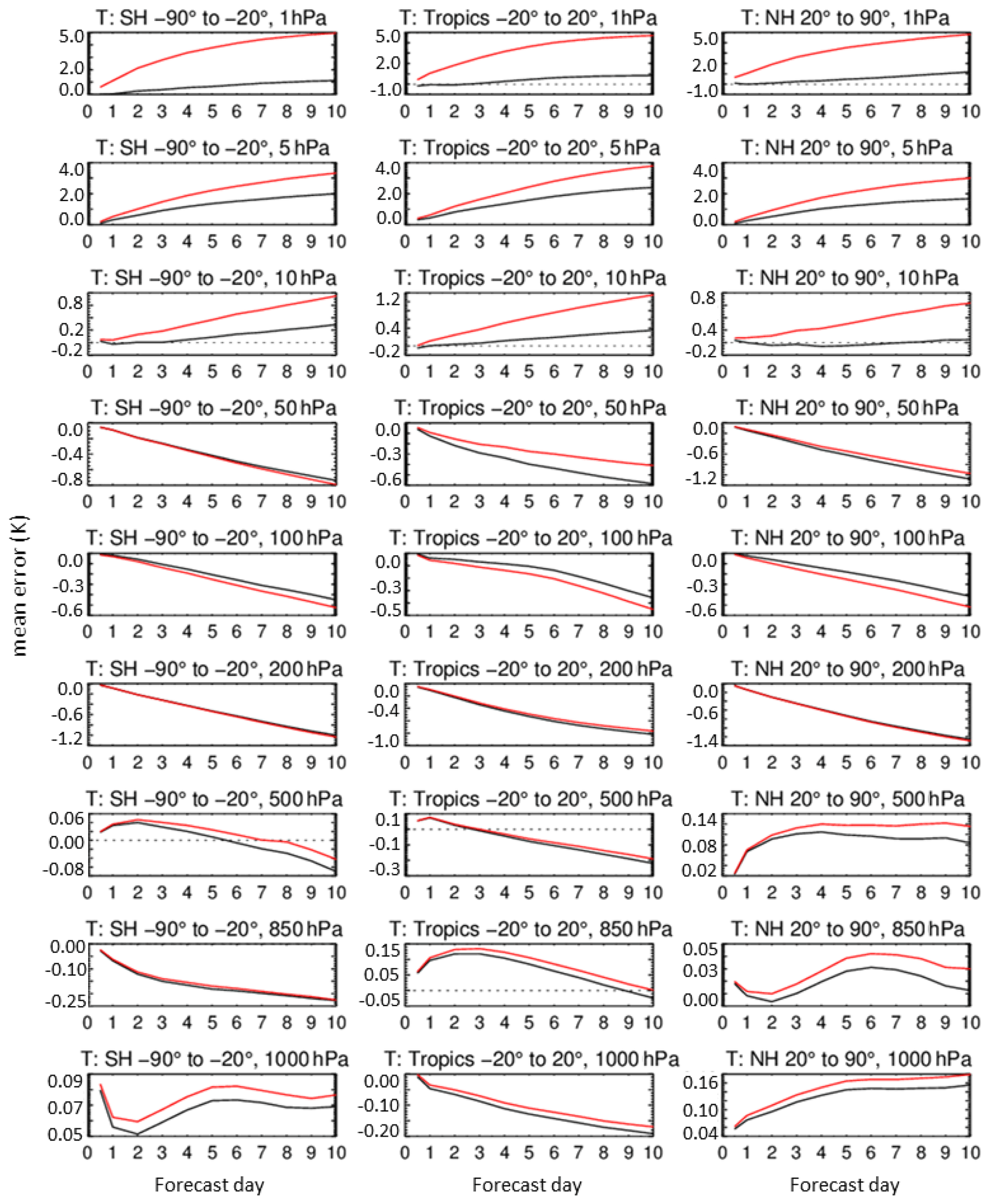
Figure 10Mean error in the temperature field (K) compared to the operational ECMWF analyses, as a function of lead time for the forecast experiment using the new BMS prognostic ozone (black) and the experiment using the ozone climatology (red) in the radiation scheme. The two 10 d forecast model runs cover a 1-year period, from August 2012 to July 2013. The figure shows three latitudinal bands, 90–20∘ S (left column), 20∘ S–20∘ N (centre column) and 20–90∘ N (right column), for different pressure levels as labelled for each row, from 1.0 to 1000 hPa.
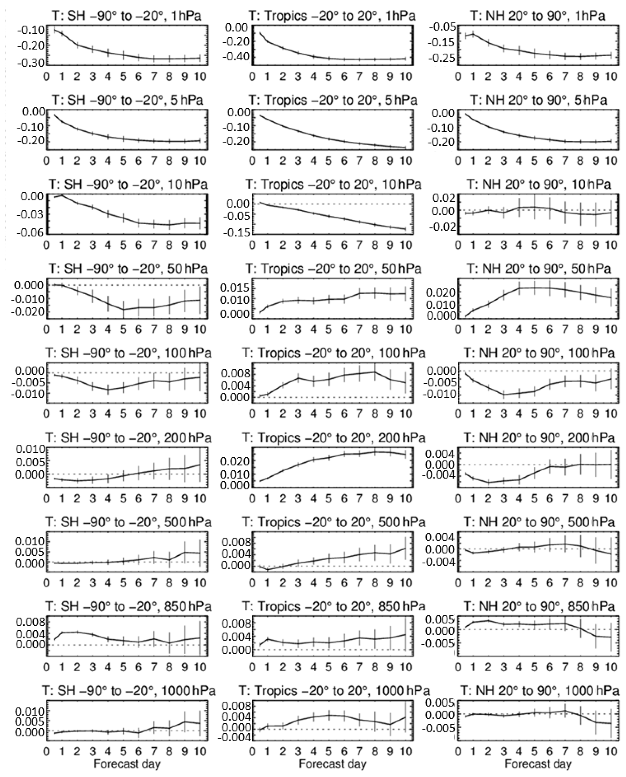
Figure 11Normalised differences in root mean square error (DRMSE), as a function of lead time, in the forecast temperature field (K) between the experiment using the new interactive ozone scheme and the experiment using the default ozone climatology within the radiation code. The forecast model runs cover a 1-year period, with 10 d forecasts from August 2012 to July 2013. The figure shows three latitudinal bands, 90–20∘ S (left column), 20∘ S–20∘ N (centre column) and 20–90∘ N (right column), for different pressure levels as labelled for each row, from 1.0 to 1000 hPa.
The rest of this paper focuses on the evaluation of meteorological impacts for experiments using the new BMS prognostic ozone compared to the control experiments using the default climatology configuration. It is worth noting that the ECMWF operational model has gone through version updates after our study, and the ozone climatology has been updated following Hogan et al. (2017). Although beyond the scope of this paper, comparison of biases for the currently operational default configuration should be a matter of future investigation.
4.2 Impacts during SSW events
The winter stratospheric variability in the NH high latitudes is dominated by the occurrence of sudden stratospheric warmings (SSWs); since these SSW events can lead to surface cold outbreaks over NH midlatitudes (e.g. Baldwin and Dunkerton, 2001; Kolstad et al., 2010; Lehtonen and Karpechko, 2016), it is important for the forecast model of an NWP system to simulate them as realistically as possible.
During the SSW that took place in early February 2016, temperature anomalies reached maximum values on 7 February 2016 between 5 and 20 hPa (e.g. Manney and Lawrence, 2016). Two medium-range forecast experiments are used to assess the role of the new ozone model in this SSW event: one using the new BMS ozone interactive with radiation and one using the default model configuration in which the radiation scheme sees an ozone climatology. These experiments cover the period 15 December 2015–14 February 2016; to compare them we show some of the diagnostics used by Diamantakis (2014).
Figure 12 shows that, with the new prognostic ozone scheme, temperature at 5 hPa becomes warmer over the Eastern Arctic region (up to 20 K warmer) compared to the default model configuration (Fig. 12a, b, d), bringing it closer to the operational analysis (Fig. 12c). We have compared t+240 h in the forecast experiments, from the 28 January forecast, against the corresponding operational analysis for the 7 February to allow for the maximum ozone response. The improvement seen at 5 hPa is also seen at lower altitude levels (figure not shown).
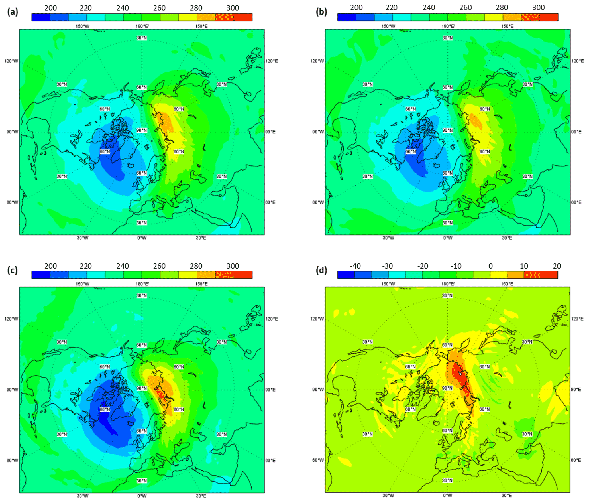
Figure 12Temperature field on 7 February 2016 at 5 hPa from (a) the forecast experiment using the new BMS ozone scheme, (b) the forecast experiment using the default ozone scheme and (c) the operational analysis. The differences between both forecast experiments (BMS – default) are shown in panel (d). For the forecast experiments the field shown corresponds to day 10 of the forecast initialised on 28 January 2016.
For these two experiments we have also examined the impact on the wind field. Figure 13 shows the change in RMSE for the vector wind velocity for different lead times, averaged over the experiment duration. The improvement in wind errors when BMS ozone is used consistently increases with lead time and is transferred from the stratosphere down to the troposphere for high latitudes from day 6. By day 10 in the forecast the error reduction in the wind field is statistically significant in the troposphere.
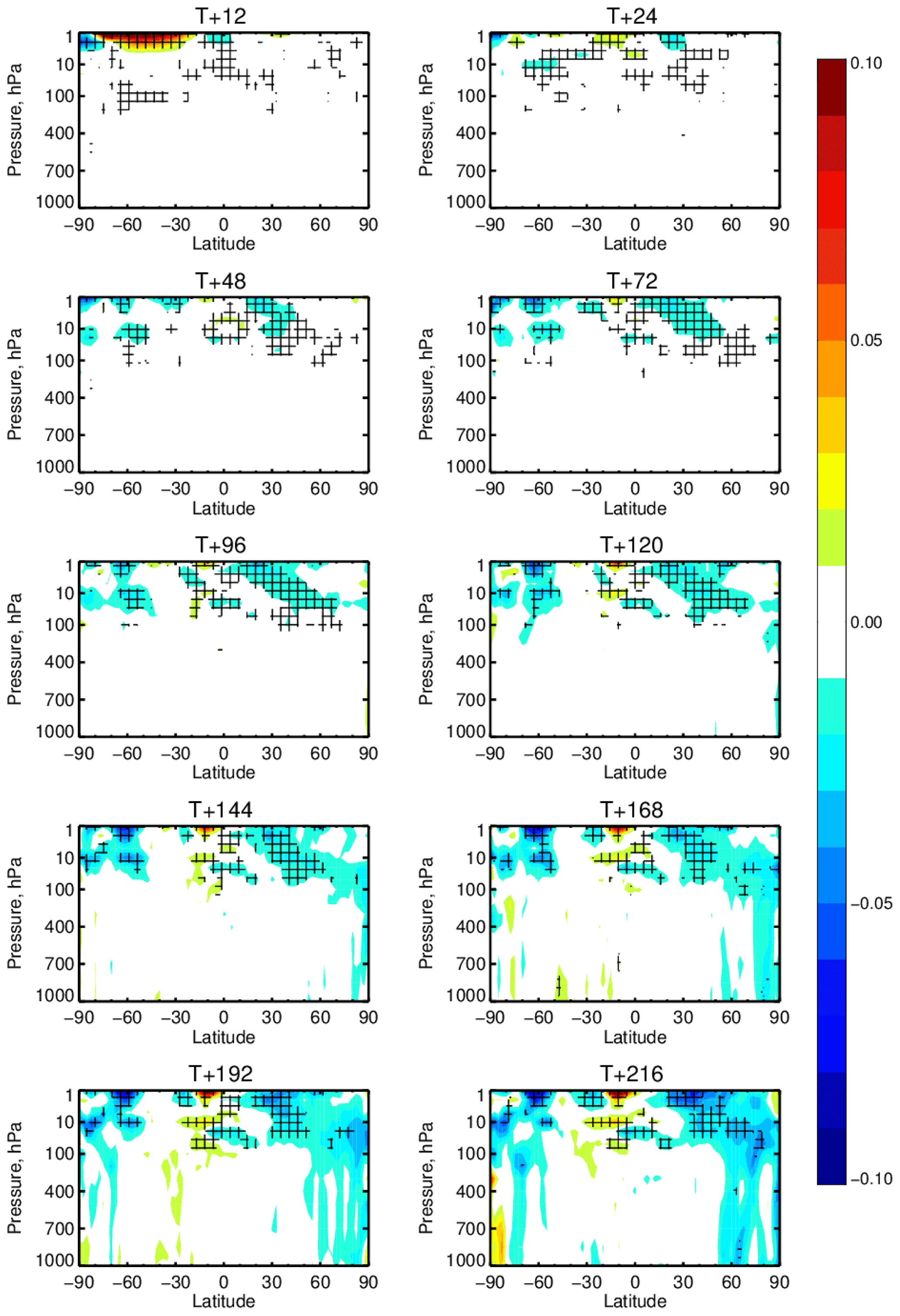
Figure 13Cross sections for the change of RMSE in the vector wind velocity (m s−1) for different lead times (24 to 240 h) for the period 15 December 2015–15 February 2016. Each experiment, one using the new ozone scheme interactive with radiation and one using the default scheme, is compared to the ECMWF operational analysis as reference for normalising the error difference; this figure displays the differences between both experiments compared to the reference. Hatched regions indicate where results are statistically significant to the 95 % confidence interval.
During SSW events, when both temperature and ozone distributions change rapidly in the stratosphere, a climatology-based ozone field cannot pass information to the radiation code that resembles the actual atmospheric situation; therefore, the model misses the potential source of tropospheric predictability that comes from the downward propagation of the stratospheric signal.
4.3 Long-range impacts
We have performed two seasonal experiments with start dates in May and November, covering the period 1981–2010, using a horizontal resolution of T255, 91 vertical levels and three ensemble members. The control experiment uses the MACC ozone climatology inside the radiation code, while the BMS experiment uses the new prognostic ozone interactive with the radiation code. Temperature differences with respect to ERA-Interim for these two experiments are shown in Fig. 14, averaged over DJF (upper panels) and MAM (lower panels).

Figure 14Zonal average of temperature differences compared to ERA-Interim for two long-range model experiments, one with the default model configuration in which the radiation scheme sees the ozone climatology (a, c) and another one in which the new ozone scheme is used and made interactive with radiation (b, d). Panels (a) and (b) show DJF differences, and panels (c) and (d) show MAM differences. The period covered is 1981–2010, and the model version used is Cy41r1 with a horizontal resolution T255 and 91 vertical levels up to 0.01 hPa. Dotted areas indicate regions in which the differences are statistically significant at the 95 % confidence level.
There is a clear improvement around 50 hPa when using the new ozone scheme for both seasons and all latitudes, especially over the SH middle and high latitudes. In these SH regions the BMS prognostic ozone reduces differences by up to 4.0 K. Also for levels above 20 hPa differences with respect to ERA-Interim are reduced, especially in the summer hemisphere, by more than 1.0 K during DJF and MAM. These results have shown that a prognostic ozone field contributes to more realistic temperatures in the SH stratosphere than a climatology, also for the seasons following the Antarctic ozone hole months.
Figure 15 shows the zonal averaged differences in zonal wind between the two experiments for the SON season to assess the impact on wind circulation during the ozone hole season (differences for other seasons were smaller or not statistically significant). The new ozone experiment shows stronger zonal winds over the Antarctic vortex edge latitudes between 20–400 hPa, which is physically linked to the lower concentrations of ozone simulated by the new scheme over this region compared to the default climatology. When comparing to ERA-Interim (figure not shown), the control run was negatively biased over this region compared to the reanalysis (up to 2 m s−1); this bias appears reduced in the BMS run. The strengthening of winds in the BMS run is also in overall agreement with findings in Son et al. (2008).
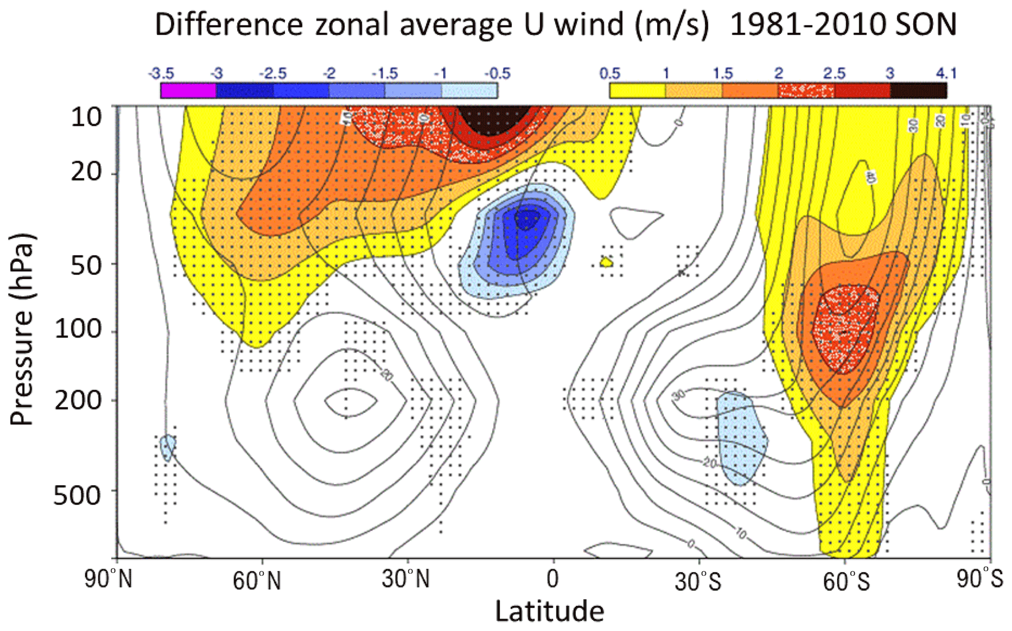
Figure 15Zonal average of differences in the zonal wind u (m s−1) between the long-range experiment using the new ozone scheme and a long-range experiment using the default configuration, for the September–October–November (SON) season. Experiments and model configurations used here are as in Fig. 14. Hatched areas indicate regions where the differences are statistically significant at the 95 % confidence interval.
Seasonal experiments performed under the Seasonal-to-decadal climate Prediction for the improvement of European Climate Services (SPECS) EU project also showed improvements in the equatorial winds and the quasi-biennial oscillation (QBO) signal when the new BMS prognostic ozone was made interactive with radiation (Knight et al., 2016).
4.3.1 North Atlantic sector
Moving to the North Atlantic sector winter, we find that the new ozone scheme improves the representation of the North Atlantic Oscillation (NAO) in the model. Figure 16 shows the level of agreement between two long-range model experiments (exp30clim and exp30bms) and ERA-Interim on representing the NAO index. The NAO index is calculated as the first empirical orthogonal function (EOF) of the geopotential height Z500 over the North Atlantic sector. The correlation value for the winter NAO index is almost doubled compared to the default configuration, increasing from 0.25 in the control experiment using the default ozone climatology (Fig. 16a) to 0.44 in the experiment with the new BMS prognostic ozone (Fig. 16b).
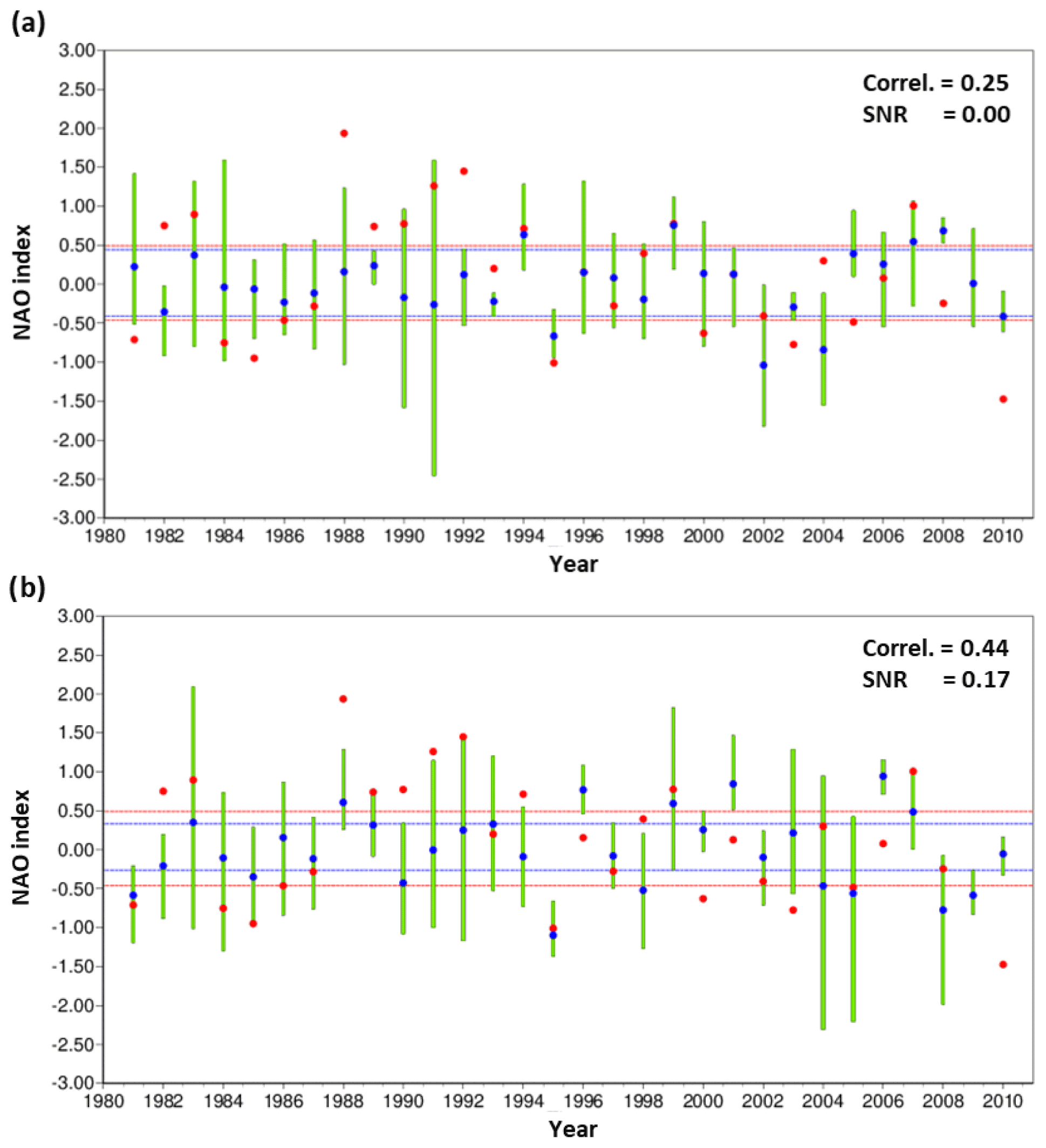
Figure 16Time series of the winter (DJF) NAO index for the long-range experiment using (a) the default configuration and (b) the experiment using the new BMS ozone, together with NAO index values from the ERA-Interim reanalysis. Red dots represent the NAO index value from ERA-Interim reanalysis, and blue dots correspond to the ensemble mean of the model runs; the green bars show the ensemble variability for each year NAO index. The NAO index is calculated as the first empirical orthogonal function (EOF) of the geopotential height Z500 over the North Atlantic sector. The correlation value between the ensemble mean NAO index and the reanalysis NAO index time series is also included in each panel, together with the signal-to-noise ratio (SNR) value for each case. The horizontal lines delimit the main tercile interval for the ensemble mean time series of the model experiments (blue) and ERA-Interim (red).
Figure 16 also includes the signal-to-noise ratio (SNR) value, defined as , where is the ensemble mean variance and is the average variance of individual ensemble members. Although we need to interpret SNR values with caution because of the ensemble size, the experiment using the BMS ozone also shows an increase in the SNR value in the North Atlantic sector, which goes from 0.00 in the control experiment to 0.17 with the new prognostic ozone.
These experiments, where the only difference is the stratospheric ozone representation, allow us to attribute the increase in NAO model performance to stratospheric sources.
A more realistic stratospheric ozone distribution improves the ozone concentration gradients between the pole and the Equator, modifying the latitudinal heating gradient in the LS region. Plausibly, this affects the altitude distribution of the tropopause in the model and therefore surface pressure gradients between low and high latitudes and the NAO signal. Future work should be done to fully assess these mechanisms, which is beyond the scope and resources of our current study.
Our results show that a more realistic stratospheric ozone field contributes to a more realistic stratosphere–troposphere coupling in the model. The links between the NAO and winter time weather over Europe are well established (e.g. Cattiaux et al., 2010; Buehler et al., 2011; Scaife et al., 2014); therefore, using a more realistic stratospheric ozone description increases the potential to exploit stratospheric sources for improved tropospheric weather prediction in the Atlantic sector.
4.3.2 Antarctic polar vortex
In the Southern Hemisphere the seasonality and interannual variability of the polar vortex and the ozone layer are closely related. To investigate this last part of our study we have had access to the new ECMWF seasonal system SEAS5 (Johnson et al., 2019). Two SEAS5 seasonal experiments are compared here: one seasonal experiment uses SEAS5 with its default configuration (ozone climatology in the radiation scheme), and the second SEAS5 experiment uses the same configuration except that ozone is replaced by the BMS prognostic ozone model interactive with radiation.
The interannual variability of the SH polar vortex is shown in Fig. 17 for these seasonal experiments initialised on 1 August over the period 1993–2015 (2002 has been excluded from the analysis shown in this figure). For each of the 22 years we randomly select an ensemble member hindcast. We then compute the interannual standard deviation of this randomly selected hindcast time series. We do this 10 000 times to produce a probability distribution (shaded envelopes in Fig. 17), and we plot the 1 %, 5 %, 25 %, 50 %, 75 %, 95 % and 99 % threshold values for each day from 1 August until 1 March.
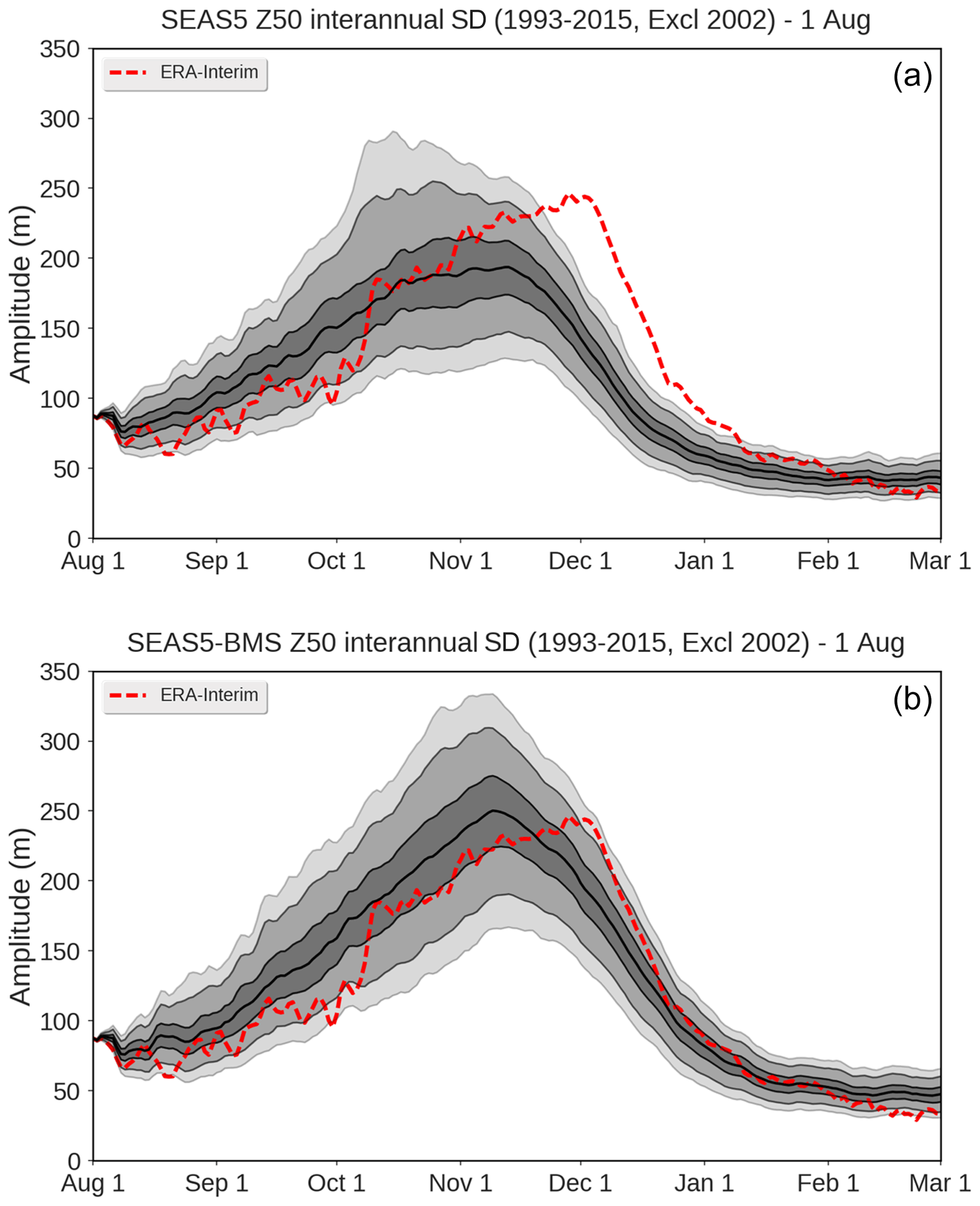
Figure 17Polar-cap geopotential height interannual standard deviation for the SEAS5 default simulation (a) and the SEAS5 simulation using the BMS ozone model (b); simulations cover the period 1993–2015 (1 August start dates have been used). The year 2002 has been excluded. The red dotted line shows corresponding values from ERA-Interim. Solid black lines show the interannual standard deviation from the model experiments, and grey shaded regions correspond to the 1 %, 5 %, 25 %, 50 %, 75 %, 95 % and 99 % threshold values for each day from 1 August until 1 March.
From the top panel in Fig. 17 it can be seen that the seasonality of the stratosphere in this region is not realistic with the default SEAS5 compared to ERA-Interim; the vortex shift-down occurs too early compared to the reanalysis. When the new BMS prognostic ozone is used, the timing of the SH polar vortex is in much better agreement with ERA-Interim, and the interannual variability increases.
Byrne and Shepherd (2018) found in their study, using ERA-Interim reanalysis, that Antarctic ozone depletion has caused a seasonal delay in the breakdown of the SH polar vortex along the period 1980–present, and they also pointed out that feedbacks between ozone and dynamics may be responsible for the increase in the interannual variability observed in the SH polar vortex. Our results with the SEAS5 experiments confirm their findings, showing that a realistic interactive prognostic ozone field is needed to reproduce the SH polar vortex behaviour, while an ozone climatology does not provide enough information for the model to reproduce all necessary feedbacks with dynamics.
Figure 18 shows the correlation of the polar-cap averaged geopotential height in the SH between the seasonal experiments used in Fig. 17 and ERA-Interim. For the period 1993–2015, excluding year 2002, the correlation patterns are similar for the standard SEAS5 and SEAS5 with BMS ozone, although the new ozone contributes to significantly larger correlation values for levels above 100 hPa in November–January. This is consistent with the more realistic timing in the polar vortex simulated with the new BMS ozone. If year 2002 is included in the analysis (lower panels in Fig. 18), the difference is, as expected, more evident. With the new ozone the correlation clearly increases during September–October–November (SON), as well as at tropospheric levels, where the default SEAS5 simulation was not showing any significant correlation. This can be explained by the ability of the new ozone model to realistically respond and feed back to the rapid dynamical changes that took place during the unusual Antarctic vortex split of year 2002; in Sect. 3.1.1 we have shown the capability of the new BMS scheme to simulate realistic ozone distributions during the 2002 Antarctic vortex split.
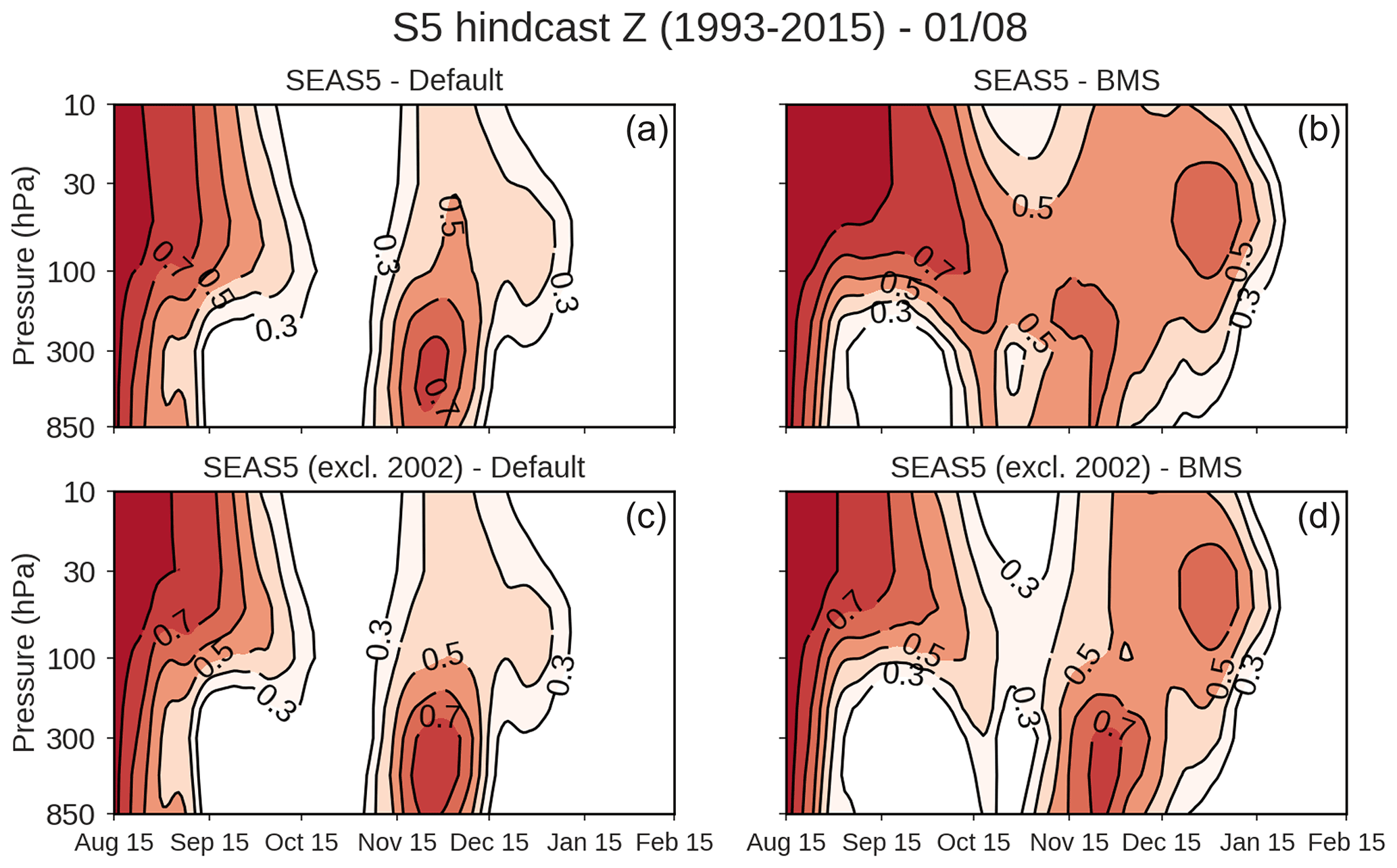
Figure 18Correlation values between 30 d mean ensemble mean SH polar-cap averaged geopotential height for the seasonal experiments and 30 d mean ERA-Interim SH polar-cap averaged geopotential height, as a function of pressure level and calendar day. Seasonal experiments are from SEAS5 default configuration (a, c) and from SEAS5 with BMS ozone (b, d). The period shown is 1993–2015 (a, b) and 1993–2015 excluding year 2002 (c, d). Coloured areas indicate statistically significant correlations at the 95 % confidence level. Darkest red colours indicate higher correlations; contour labels increase by 0.1.
Results in Fig. 18 demonstrate that using a stratospheric ozone model capable of reproducing realistic evolution of ozone vertical concentrations also improves meteorological fields, both on average over the whole period considered, 1993–2015, and also during very unusual meteorological events such as the 2002 Antarctic vortex split.
A model without a realistic description of stratospheric ozone underestimates the role of the stratosphere in shaping tropospheric meteorological fields at different timescales.
In this section we summarise the main findings of our study and discuss further work plans and recommendations deriving from our investigations.
5.1 Summary
We have implemented the stratospheric ozone model by Monge-Sanz et al. (2011) (also known as the BMS model) in the ECMWF system, compared its performance to that of the default ozone used by ECMWF, and assessed its impacts on meteorological fields at medium-range and seasonal timescales.
The BMS scheme is the first stratospheric ozone linear model that consistently accounts for heterogeneous chemistry (e.g. ozone destruction due to polar stratospheric clouds), instead of using a separate ad hoc term, providing a more realistic link with temperature and radiation. The new approach is in better agreement with the current scientific knowledge of chemical and physical processes that affect stratospheric ozone (World Meteorological Organization, 2019) than approaches adopted by previous linear ozone models (McLinden et al., 2000; McCormack et al., 2006; Cariolle and Teyssèdre, 2007).
The present study is, to the best of our knowledge, the first time that the impacts of a stratospheric ozone model are assessed at different NWP timescales to evaluate its performance towards its implementation in a seamless model system. We have shown that the new scheme provides significantly better ozone distribution and variability in the ECMWF model than the currently default ozone configuration, showing particularly good agreement with observations over the high southern latitudes and the ozone hole season, even during the unusual atmospheric conditions of the 2002 Antarctic vortex split.
When used interactively with radiation in the ECMWF model, the BMS ozone scheme reduces stratospheric temperature biases both for medium-range and seasonal timescales, compared to the default ECMWF model configuration in which the radiation scheme uses an ozone climatology, and improves temperature and wind fields during Arctic SSWs.
We have also shown that the BMS ozone improves the NAO signal in seasonal model runs, therefore contributing to a more realistic stratosphere–troposphere coupling in the model. The interannual variability and seasonality of the SH polar vortex is also improved when using the BMS ozone model in runs performed with the ECMWF seasonal system (SEAS5), compared to the default SEAS5 configuration which uses an ozone climatology. All this demonstrates that the BMS scheme is realistically linked to temperature and dynamics and therefore well prepared to adapt and feed back to rapid changes in meteorology. The same adaptability cannot be achieved with an ozone climatology in the radiation scheme.
Our results also provide evidence for the need of a realistic prognostic stratospheric ozone field in ESMs for these models to perform more accurately at different timescales. The realistic stratospheric concentration values obtained with the BMS scheme, as well as its high adaptability to both usual and unusual meteorological conditions at different timescales together with its low computational cost, make the BMS scheme an excellent option to model stratospheric ozone within ESMs. The BMS scheme is able to model stratospheric ozone with a degree of complexity that provides realistic stratospheric ozone distributions, of comparable quality to the ozone field from world-leading full-chemistry models, while keeping low computational costs suitable for resolution and production times required for weather forecasting (both at medium-range and seasonal timescales). Future work should also investigate the performance of the BMS scheme within other global models and exploit its benefits for different ESMs applications beyond medium-range NWP and seasonal prediction into climate timescales.
Next, we briefly discuss ongoing further developments of the BMS model version we have used here and how they are expected to improve the results obtained with the current version. We also provide a summary of benefits that the implementation of a realistic prognostic stratospheric ozone brings to seamless Earth system models, from medium-range NWP forecasts to seasonal prediction and reanalysis production.
5.2 Ongoing and future work
To tackle the tropical bias exhibited in model runs with the BMS scheme, Monge-Sanz et al. (2011) tested the use of a different climatology reference based on observations, and although results improved over the tropics (Fig. 7 in their paper), concentrations over high latitudes were degraded by the different climatology. More recent versions of the parent full-chemistry CTM have solved the tropical bias issue and can now be used to derive a new version of the climatology terms that would not suffer from this tropical negative bias. To reduce differences with observations at high latitudes, the scheme could use coefficients that are provided twice a month, instead of just on the 15th of each month, which allow us to simulate more realistic loss rates for the sunlight levels found in the polar early spring. As a further method to improve the simulation of ozone distributions, unlike the default CD scheme, the BMS scheme coefficients could be provided in a 3D grid, instead of 2D averaged values, to also account for intrinsic longitudinal variations in ozone chemistry. Following the method by Monge-Sanz et al. (2011) a newer version of the parent CTM can be used to compute a more advanced version of the BMS ozone scheme. This newly derived version can be obtained at higher horizontal and vertical resolution, and the tendencies can be computed with CTM runs driven by more accurate meteorology, e.g. from ERA-5 reanalysis fields. Solar effects are now also part of the latest CTM version; thus, solar variability effects can also be incorporated in the linear ozone model by deriving tendencies corresponding to solar maxima and solar minima conditions. The production of this new version of the BMS scheme is now part of ongoing work. As additional future developments the ozone scheme can also include higher-order terms to take into account second-order nonlinear effects, as well as links to other main stratospheric species like chlorofluorocarbons (CFCs) and CH4 Monge-Sanz et al. (2013).
5.2.1 Tropospheric ozone treatment
The ozone model discussed in this study, as other ozone linear schemes like the default one used by the ECMWF system, are designed for the stratosphere; their use is not recommended for the tropospheric region, where ozone is affected by highly nonlinear processes involving pollutants and ozone precursors. A realistic representation of tropospheric ozone is the full-chemistry approach, but this is still unviable for operational high-resolution models due to high computational costs. Alternatives for representing tropospheric ozone include the use of an up-to-date climatology based on observations or reanalysis that would be merged to the prognostic ozone in the stratosphere.
5.2.2 Benefits for seamless Earth system models
A realistic stratosphere is increasingly recognised as one of the keys to develop seamless Earth system models, due to the role it plays for tropospheric processes at different timescales, from weather to climate. The ozone model in our study is a valuable contribution to achieve seamless use of emerging ESMs, as it offers similar accuracy to a full-chemistry model for stratospheric ozone, allowing for ozone–climate feedbacks that level with those provided by current chemistry-climate models (CCMs) with interactive stratospheric ozone, while keeping the computational cost affordable for weather forecast applications and resolutions.
Additionally, by implementing a realistic scheme for prognostic ozone, and ideally also for other radiative active gases in the stratosphere (see e.g. Monge-Sanz et al., 2013), the system will be better prepared for the eventual operational use of interactive full chemistry, as several feedbacks within the model will already have been investigated with the ozone model we propose, allowing for compensation errors to be identified and possibly eliminated.
5.2.3 Benefits for long reanalyses
Long reanalyses have become an essential part of weather and climate scientific research and applications. Recent major international projects, like the SPARC (Stratosphere-troposphere Processes and their Role in Climate) Reanalysis Intercomparison Project (SRIP), part of the World Climate Research Program (WCRP) core activities, have identified areas that will need more attention in the production of future reanalyses in order to represent a more realistic stratosphere (Fujiwara et al., 2017). The representation of stratospheric ozone in the atmospheric models used to produce the reanalyses is one of these aspects (Monge-Sanz et al., 2021). The adaptability shown by the new BMS ozone scheme to very different meteorological conditions makes it an excellent candidate for future Earth system reanalyses. Such reanalyses will need climate forcings and stratospheric feedbacks to be accurately included; thus, stratospheric ozone descriptions that realistically respond, and feed back, to changes in temperature and dynamics will be essential to correctly account for trends in stratospheric ozone depletion and recovery levels.
Observation datasets used in this study are available as stated in the corresponding references included in the article. The IFS code is available subject to a licence agreement with ECMWF. The BMS model coefficients are available for research purposes from the corresponding author upon request. The model experiments data from this work are archived on the Meteorological Archival and Retrieval System (MARS) of ECMWF, which is available to users with a registered access. Interested readers with no registered access can obtain more information or data from the corresponding author upon request. Reanalysis data are also available from the MARS archiving system of ECMWF (https://apps.ecmwf.int/archive-catalogue/, last access: 12 January 2021; ECMWF, 2022).
BMMS designed the study; implemented the new ozone scheme in the ECMWF system; performed experiments, results validation and interpretation; wrote the paper; and coordinated co-authors’ contributions. AB, NB, MD, JF, LM, IP and AW contributed to data analysis and results interpretation. LM and IP also contributed to performance of seasonal experiments. LJ designed the visualisation tool used for validation against ozone profile observations. LJG, RJH, NW, MPC and TGS provided insightful feedback and contributed to review draft versions of the manuscript.
The contact author has declared that neither they nor their co-authors have any competing interests.
Publisher’s note: Copernicus Publications remains neutral with regard to jurisdictional claims in published maps and institutional affiliations.
This study was partially funded by the MACC-II and SPECS FP7 EU projects. Beatriz M. Monge-Sanz and Lesley J. Gray also acknowledge funding from the UK Natural Environment Research Council (NERC) through the ACSIS project (North Atlantic Climate System Integrated Study) led by the National Centre for Atmospheric Science (NCAS). The first author is very grateful to Adrian Simmons, Agathe Untch and Jean-Jacques Morcrette for many helpful discussions and their valuable initial guidance with the ECMWF system; special thanks are also due to Franco Molteni for useful discussions during the preparation of this paper. We also thank Paul Burton, Gabor Radnoti and the ECMWF User Support team for their help with the IFS technical environment. We would also like to thank the editor and two anonymous reviewers for constructive comments that have contributed to enhance the quality of the paper.
This paper was edited by Farahnaz Khosrawi and reviewed by two anonymous referees.
Badia, A., Jorba, O., Voulgarakis, A., Dabdub, D., Pérez García-Pando, C., Hilboll, A., Gonçalves, M., and Janjic, Z.: Description and evaluation of the Multiscale Online Nonhydrostatic AtmospheRe CHemistry model (NMMB-MONARCH) version 1.0: gas-phase chemistry at global scale, Geosci. Model Dev., 10, 609–638, https://doi.org/10.5194/gmd-10-609-2017, 2017. a, b
Baldwin, M. P. and Dunkerton, T. J.: Stratospheric Harbingers of Anomalous Weather Regimes, Science, 294, 581–584, https://doi.org/10.1126/science.1063315, 2001. a
Buehler, T., Raible, C. C., and Stocker, T. F.: The relationship of winter season North Atlantic blocking frequencies to extreme cold or dry spells in the ERA-40, Tellus A, 63, 174–187, https://doi.org/10.1111/j.1600-0870.2010.00492.x, 2011. a
Butler, A. H., Sjoberg, J. P., Seidel, D. J., and Rosenlof, K. H.: A sudden stratospheric warming compendium, Earth Syst. Sci. Data, 9, 63–76, https://doi.org/10.5194/essd-9-63-2017, 2017. a
Byrne, N. J. and Shepherd, T. G.: Seasonal Persistence of Circulation Anomalies in the Southern Hemisphere Stratosphere and Its Implications for the Troposphere, J. Climate, 31, 3467–3483, https://doi.org/10.1175/JCLI-D-17-0557.1, 2018. a
Cariolle, D. and Déqué, M.: Southern Hemisphere Medium-Scale Waves and Total Ozone Disturbances in a Spectral General Circulation Model, J. Geophys. Res., 91, 10825–10846, 1986. a
Cariolle, D. and Teyssèdre, H.: A revised linear ozone photochemistry parameterization for use in transport and general circulation models: multi-annual simulations, Atmos. Chem. Phys., 7, 2183–2196, https://doi.org/10.5194/acp-7-2183-2007, 2007. a, b, c
Cattiaux, J., Vautard, R., Cassou, C., Yiou, P., Masson-Delmotte, V., and Codron, F.: Winter 2010 in Europe: A cold extreme in a warming climate, Geophys. Res. Lett., 37, L20704, https://doi.org/10.1029/2010GL044613, 2010. a
Dee, D. P., Uppala, S. M., Simmons, A. J., Berrisford, P., Poli, P., Kobayashi, S., Andrae, U., Balmaseda, M. A., Balsamo, G., Bauer, P., Bechtold, P., Beljaars, A. C. M., van de Berg, L., Bidlot, J., Bormann, N., Delsol, C., Dragani, R., Fuentes, M., Geer, A. J., Haimberger, L., Healy, S., Hersbach, H., Hólm, E. V., Isaksen, L., Kållberg, P., Köhler, M., Matricardi, M., McNally, A. P., Monge-Sanz, B. M., Morcrette, J.-J., Peubey, C., de Rosnay, P., Tavolato, C., Thépaut, J.-N., and Vitart, F.: The ERA-Interim reanalysis: Configuration and performance of the data assimilation system, Q. J. Roy. Meteor. Soc., 137, 553–597, https://doi.org/10.1002/qj.828, 2011. a, b
Diamantakis, M.: Improving ECMWF forecasts of sudden stratospheric warmings, ECMWF Newsletter, 141, 30–36, https://doi.org/10.21957/pq2zizgf, 2014. a, b
ECMWF: Archive Catalogue, ECMWF Reanalysis data, ECMWF [data set], https://apps.ecmwf.int/archive-catalogue/ (last access: 12 January 2021), 2022.
Eyring, V., Waugh, D. W., Bodeker, G. E., Cordero, E., Akiyoshi, H., Austin, J., Beagley, S. R., Boville, B. A., Braesicke, P., Brühl, C., Butchart, N., Chipperfield, M. P., Dameris, M., Deckert, R., Deushi, M., Frith, S. M., Garcia, R. R., Gettelman, A., Giorgetta, M. A., Kinnison, D. E., Mancini, E., Manzini, E., Marsh, D. R., Matthes, S., Nagashima, T., Newman, P. A., Nielsen, J. E., Pawson, S., Pitari, G., Plummer, D. A., Rozanov, E., Schraner, M., Scinocca, J. F., Semeniuk, K., Shepherd, T. G., Shibata, K., Steil, B., Stolarski, R. S., Tian, W., and Yoshiki, M.: Multimodel projections of stratospheric ozone in the 21st century, J. Geophys. Res., 112, D16303, https://doi.org/10.1029/2006JD008332, 2007. a
Flemming, J., Benedetti, A., Inness, A., Engelen, R. J., Jones, L., Huijnen, V., Remy, S., Parrington, M., Suttie, M., Bozzo, A., Peuch, V.-H., Akritidis, D., and Katragkou, E.: The CAMS interim Reanalysis of Carbon Monoxide, Ozone and Aerosol for 2003–2015, Atmos. Chem. Phys., 17, 1945–1983, https://doi.org/10.5194/acp-17-1945-2017, 2017. a, b, c
Fujiwara, M., Wright, J. S., Manney, G. L., Gray, L. J., Anstey, J., Birner, T., Davis, S., Gerber, E. P., Harvey, V. L., Hegglin, M. I., Homeyer, C. R., Knox, J. A., Krüger, K., Lambert, A., Long, C. S., Martineau, P., Molod, A., Monge-Sanz, B. M., Santee, M. L., Tegtmeier, S., Chabrillat, S., Tan, D. G. H., Jackson, D. R., Polavarapu, S., Compo, G. P., Dragani, R., Ebisuzaki, W., Harada, Y., Kobayashi, C., McCarty, W., Onogi, K., Pawson, S., Simmons, A., Wargan, K., Whitaker, J. S., and Zou, C.-Z.: Introduction to the SPARC Reanalysis Intercomparison Project (S-RIP) and overview of the reanalysis systems, Atmos. Chem. Phys., 17, 1417–1452, https://doi.org/10.5194/acp-17-1417-2017, 2017. a
Haase, S., Fricke, J., Kruschke, T., Wahl, S., and Matthes, K.: Sensitivity of the Southern Hemisphere circumpolar jet response to Antarctic ozone depletion: prescribed versus interactive chemistry, Atmos. Chem. Phys., 20, 14043–14061, https://doi.org/10.5194/acp-20-14043-2020, 2020. a
Hanson, D. and Mauersberger, K.: Laboratory studies of the nitric acid trihydrate: Implications for the South Polar stratosphere, Geophys. Res. Lett., 15, 855–858, 1988. a
Harris, N. R. P., Carpenter, L. J., Lee, J. D., Vaughan, G., Filus, M. T., Jones, R. L., OuYang, B., Pyle, J. A., Robinson, A. D., Andrews, S. J., Lewis, A. C., Minaeian, J., Vaughan, A., Dorsey, J. R., Gallagher, M. W., Breton, M. L., Newton, R., Percival, C. J., Ricketts, H. M. A., Bauguitte, S. J. B., Nott, G. J., Wellpott, A., Ashfold, M. J., Flemming, J., Butler, R., Palmer, P. I., Kaye, P. H., Stopford, C., Chemel, C., Boesch, H., Humpage, N., Vick, A., MacKenzie, A. R., Hyde, R., Angelov, P., Meneguz, E., and Manning, A. J.: Coordinated Airborne Studies in the Tropics (CAST), B. Am. Meteorol. Soc., 98, 145–162, https://doi.org/10.1175/BAMS-D-14-00290.1, 2017. a
Hogan, R., Ahlgrimm, M., Balsamo, G., Beljaars, A., Berrisford, P., Bozzo, A., Giuseppe, F. D., Forbes, R. M., Haiden, T., Lang, S., Mayer, M., Polichtchouk, I., Sandu, I., Vitart, F., and Wedi, N.: Radiation in Numerical Weather Prediction, European Centre for Medium-Range Weather Forecasts (ECMWF), Reading, U.K., Tech. Mem. No. 816, https://doi.org/10.21957/2bd5dkj8x, 2017. a
Inness, A., Baier, F., Benedetti, A., Bouarar, I., Chabrillat, S., Clark, H., Clerbaux, C., Coheur, P., Engelen, R. J., Errera, Q., Flemming, J., George, M., Granier, C., Hadji-Lazaro, J., Huijnen, V., Hurtmans, D., Jones, L., Kaiser, J. W., Kapsomenakis, J., Lefever, K., Leitão, J., Razinger, M., Richter, A., Schultz, M. G., Simmons, A. J., Suttie, M., Stein, O., Thépaut, J.-N., Thouret, V., Vrekoussis, M., Zerefos, C., and the MACC team: The MACC reanalysis: an 8 yr data set of atmospheric composition, Atmos. Chem. Phys., 13, 4073–4109, https://doi.org/10.5194/acp-13-4073-2013, 2013. a
Jeong, G.-R., Monge-Sanz, B. M., Lee, E.-H., and Ziemke, J. R.: Simulation of stratospheric ozone in global forecast model using linear photochemistry parameterization, Asia-Pac. J. Atmos. Sci., 52, 479–494, https://doi.org/10.1007/s13143-016-0032-x, 2016. a, b
Johnson, S. J., Stockdale, T. N., Ferranti, L., Balmaseda, M. A., Molteni, F., Magnusson, L., Tietsche, S., Decremer, D., Weisheimer, A., Balsamo, G., Keeley, S. P. E., Mogensen, K., Zuo, H., and Monge-Sanz, B. M.: SEAS5: the new ECMWF seasonal forecast system, Geosci. Model Dev., 12, 1087–1117, https://doi.org/10.5194/gmd-12-1087-2019, 2019. a, b
Kang, S. M., Polvani, L. M., Fyfe, J. C., and Sigmond, M.: Impact of polar ozone depletion on subtropical precipitation, Science, 332, 951–954, 2011. a
Knight, J., Andrews, M., Stockdale, T., Monge-Sanz, B., Déqué, M., Guérémy, J.-F., Saint-Martin, D., Caian, M., and Orsolini, Y.: Sensitivity to improvements in stratospheric processes and variations in solar forcings, SPECS Report Deliverable D43.1, https://www.specs-fp7.eu/sites/default/files/u1/SPECS_D43.1.pdf (last access: 21 February 2022), 2016. a, b
Kolstad, E. W., Breiteig, T., and Scaife, A. A.: The association between stratospheric weak polar vortex events and cold air outbreaks in the Northern Hemisphere, Q. J. Roy. Meteor. Soc., 136, 886–893, https://doi.org/10.1002/qj.620, 2010. a, b
Kretschmer, M., Coumou, D., Agel, L., Barlow, M., Tziperman, E., and Cohen, J.: More-Persistent Weak Stratospheric Polar Vortex States Linked to Cold Extremes, B. Am. Meteorol. Soc., 99, 49–60, https://doi.org/10.1175/BAMS-D-16-0259.1, 2018. a
Krüger, K., Naujokat, B., and Labitzke, K.: The Unusual Midwinter Warming in the Southern Hemisphere Stratosphere 2002: A Comparison to Northern Hemisphere Phenomena, J. Atmos. Sci., 62, 603–613, https://doi.org/10.1175/JAS-3316.1, 2005. a
Lehtonen, I. and Karpechko, A. Y.: Observed and modeled tropospheric cold anomalies associated with sudden stratospheric warmings, J. Geophys. Res.-Atmos., 121, 1591–1610, https://doi.org/10.1002/2015JD023860, 2016. a
Manney, G. L. and Lawrence, Z. D.: The major stratospheric final warming in 2016: dispersal of vortex air and termination of Arctic chemical ozone loss, Atmos. Chem. Phys., 16, 15371–15396, https://doi.org/10.5194/acp-16-15371-2016, 2016. a, b
Manney, G. L., Daffer, W. H., Strawbridge, K. B., Walker, K. A., Boone, C. D., Bernath, P. F., Kerzenmacher, T., Schwartz, M. J., Strong, K., Sica, R. J., Krüger, K., Pumphrey, H. C., Lambert, A., Santee, M. L., Livesey, N. J., Remsberg, E. E., Mlynczak, M. G., and Russell III, J. R.: The high Arctic in extreme winters: vortex, temperature, and MLS and ACE-FTS trace gas evolution, Atmos. Chem. Phys., 8, 505–522, https://doi.org/10.5194/acp-8-505-2008, 2008. a
McCormack, J. P., Eckermann, S. D., Siskind, D. E., and McGee, T. J.: CHEM2D-OPP: A new linearized gas-phase ozone photochemistry parameterization for high-altitude NWP and climate models, Atmos. Chem. Phys., 6, 4943–4972, https://doi.org/10.5194/acp-6-4943-2006, 2006. a
McLinden, C. A., Olsen, S. C., Hannegan, B., Wild, O., and Prather, M. J.: Stratospheric Ozone in 3-D Models: A simple chemistry and the cross-tropopause flux, J. Geophys. Res., 105, 14635–14665, 2000. a
Monge-Sanz, B. M., Chipperfield, M. P., Cariolle, D., and Feng, W.: Results from a new linear O3 scheme with embedded heterogeneous chemistry compared with the parent full-chemistry 3-D CTM, Atmos. Chem. Phys., 11, 1227–1242, https://doi.org/10.5194/acp-11-1227-2011, 2011. a, b, c, d, e, f, g, h, i, j, k, l, m, n, o, p, q, r
Monge-Sanz, B. M., Chipperfield, M. P., Untch, A., Morcrette, J.-J., Rap, A., and Simmons, A. J.: On the uses of a new linear scheme for stratospheric methane in global models: water source, transport tracer and radiative forcing, Atmos. Chem. Phys., 13, 9641–9660, https://doi.org/10.5194/acp-13-9641-2013, 2013. a, b
Monge-Sanz, B. M., Birner, T., Chabrillat, S., Diallo, M., Haenel, F., Konopka, P., Legras, B., Ploeger, F., Reddmann, T., Stiller, G., Wright, J. S., Abalos, M., Boenisch, H. Davis, S., Garny, H., Hitchcock, P., Miyazaki, K., Roscoe., H., Sato, K., Tao, M. C., and Waugh, D.: Brewer-Dobson Circulation in the SPARC Reanalyses Intercomparison Project (SRIP), SPARC Reanalyses Intercomparison Project Report No. 10, chap. 5, https://www.sparc-climate.org/wp-content/uploads/sites/5/2022/01/05_S-RIP_Report_Ch05.pdf (last access: 12 March 2022), 2021. a
Morgenstern, O., Hegglin, M. I., Rozanov, E., O'Connor, F. M., Abraham, N. L., Akiyoshi, H., Archibald, A. T., Bekki, S., Butchart, N., Chipperfield, M. P., Deushi, M., Dhomse, S. S., Garcia, R. R., Hardiman, S. C., Horowitz, L. W., Jöckel, P., Josse, B., Kinnison, D., Lin, M., Mancini, E., Manyin, M. E., Marchand, M., Marécal, V., Michou, M., Oman, L. D., Pitari, G., Plummer, D. A., Revell, L. E., Saint-Martin, D., Schofield, R., Stenke, A., Stone, K., Sudo, K., Tanaka, T. Y., Tilmes, S., Yamashita, Y., Yoshida, K., and Zeng, G.: Review of the global models used within phase 1 of the Chemistry–Climate Model Initiative (CCMI), Geosci. Model Dev., 10, 639–671, https://doi.org/10.5194/gmd-10-639-2017, 2017. a
Nakajima, H., Wohltmann, I., Wegner, T., Takeda, M., Pitts, M. C., Poole, L. R., Lehmann, R., Santee, M. L., and Rex, M.: Polar stratospheric cloud evolution and chlorine activation measured by CALIPSO and MLS, and modeled by ATLAS, Atmos. Chem. Phys., 16, 3311–3325, https://doi.org/10.5194/acp-16-3311-2016, 2016. a
Orr, A., Bracegirdle, T. J., Hosking, J. S., Jung, T., Haigh, J. D., Phillips, T., and Feng, W.: Possible Dynamical Mechanisms for Southern Hemisphere Climate Change due to the Ozone Hole, J. Atmos. Sci., 69, 2917–2932, https://doi.org/10.1175/JAS-D-11-0210.1, 2012. a
Polvani, L. M., Waugh, D. W., Correa, G. J. P., and Son, S.-W.: Stratospheric Ozone Depletion: The Main Driver of Twentieth-Century Atmospheric Circulation Changes in the Southern Hemisphere, J. Climate, 24, 795–812, https://doi.org/10.1175/2010JCLI3772.1, 2011. a
Roscoe, H. K., Shanklin, J. D., and Colwell, S. R.: Has the Antarctic Vortex Split before 2002?, J. Atmos. Sci., 62, 581–588, https://doi.org/10.1175/JAS-3331.1, 2005. a
Scaife, A. A., Arribas, A., Blockley, E., Brookshaw, A., Clark, R. T., Dunstone, N., Eade, R., Fereday, D., Folland, C. K., Gordon, M., Hermanson, L., Knight, J. R., Lea, D. J., MacLachlan, C., Maidens, A., Martin, M., Peterson, A. K., Smith, D., Vellinga, M., Wallace, E., Waters, J., and Williams, A.: Skillful long-range prediction of European and North American winters, Geophys. Res. Lett., 41, 2514–2519, https://doi.org/10.1002/2014GL059637, 2014. a
Scaife, A. A., Karpechko, A. Y., Baldwin, M. P., Brookshaw, A., Butler, A. H., Eade, R., Gordon, M., MacLachlan, C., Martin, N., Dunstone, N., and Smith, D.: Seasonal winter forecasts and the stratosphere, Atmos. Sci. Lett., 17, 51–56, https://doi.org/10.1002/asl.598, 2016. a
Schulz, A., Rex, M., Harris, N. R. P., Braathen, G. O., Reimer, E., Alfier, R., Kilbane-Dawe, I., Eckermann, S., Allaart, M., Alpers, M., Bojkov, B., Cisneros, J., Claude, H., Cuevas, E., Davies, J., De Backer, H., Dier, H., Dorokhov, V., Fast, H., Godin, S., Johnson, B., Kois, B., Kondo, Y., Kosmidis, E., Kyrö, E., Litynska, Z., Mikkelsen, I. S., Molyneux, M. J., Murphy, G., Nagai, T., Nakane, H., O'Connor, F., Parrondo, C., Schmidlin, F. J., Skrivankova, P., Varotsos, C., Vialle, C., Viatte, P., Yushkov, V., Zerefos, C., and von der Gathen, P.: Arctic ozone loss in threshold conditions: Match observations in 1997/1998 and 1998/1999, J. Geophys. Res.-Atmos., 106, 7495–7503, https://doi.org/10.1029/2000JD900653, 2001. a
Searle, K. R., Chipperfield, M. P., Bekki, S., and Pyle, J. A.: The impact of spatial averaging on calculated polar ozone loss 2. Theoretical analysis, J. Geophys. Res., 103, 25409–25416, 1998. a
Solomon, S., Haskins, J., Ivy, D. J., and Min, F.: Fundamental differences between Arctic and Antarctic ozone depletion, P. Natl. Acad. Sci. USA, 111, 6220–6225, https://doi.org/10.1073/pnas.1319307111, 2014. a
Son, S.-W., Polvani, L., Waugh, D., Akiyoshi, H., Garcia, R., Kinnison, D., Pawson, S., Rozanov, E., Shepherd, T., and Shibata, K.: The impact of stratospheric ozone recovery in the Southern Hemisphere westerly jet, Science, 320, 1486–1489, 2008. a
Strahan, S. E., Douglass, A. R., and Steenrod, S. D.: Chemical and dynamical impacts of stratospheric sudden warmings on Arctic ozone variability, J. Geophys. Res.-Atmos., 121, 11836–11851, https://doi.org/10.1002/2016JD025128, 2016. a, b
Thompson, A. M., Witte, J. C., Sterling, C., Jordan, A., Johnson, B. J., Oltmans, S. J., Fujiwara, M., Vömel, H., Allaart, M., Piters, A., Coetzee, G. J. R., Posny, F., Corrales, E., Diaz, J. A., Félix, C., Komala, N., Lai, N., Ahn Nguyen, H. T., Maata, M., Mani, F., Zainal, Z., Ogino, S.-Y., Paredes, F., Penha, T. L. B., da Silva, F. R., Sallons-Mitro, S., Selkirk, H. B., Schmidlin, F. J., Stübi, R., and Thiongo, K.: First Reprocessing of Southern Hemisphere Additional Ozonesondes (SHADOZ) Ozone Profiles (1998–2016): 2. Comparisons With Satellites and Ground-Based Instruments, J. Geophys. Res.-Atmos., 122, 13000–13025, https://doi.org/10.1002/2017JD027406, 2017. a
Tritscher, I., Pitts, M. C., Poole, L. R., Alexander, S. P., Cairo, F., Chipperfield, M. P., Grooß, J.-U., Höpfner, M., Lambert, A., Luo, B., Molleker, S., Orr, A., Salawitch, R., Snels, M., Spang, R., Woiwode, W., and Peter, T.: Polar Stratospheric Clouds: Satellite Observations, Processes, and Role in Ozone Depletion, Rev. Geophys., 59, e2020RG000702, https://doi.org/10.1029/2020RG000702, 2021. a, b
Waugh, D. W., Sobel, A. H., and Polvani, L. M.: What Is the Polar Vortex and How Does It Influence Weather?, B. Am. Meteorol. Soc., 98, 37–44, https://doi.org/10.1175/BAMS-D-15-00212.1, 2017. a
World Meteorological Organization (WMO): Scientific Assessment of Ozone Depletion: 2018, Global Ozone Research and Monitoring Project-Report No. 58, Geneva, Switzerland, https://ozone.unep.org/sites/default/files/2019-05/SAP-2018-Assessment-report.pdf (last access: 21 February 2022), 2019. a, b