the Creative Commons Attribution 4.0 License.
the Creative Commons Attribution 4.0 License.
 | 22 Mar 2022
Novel assessment of numerical forecasting model relative humidity with satellite probabilistic estimates
Hélène Brogniez
Pierre-Emmanuel Kirstetter
Philippe Chambon
A novel method of comparison between an atmospheric model and satellite probabilistic estimates of relative humidity (RH) in the tropical atmosphere is presented. The method is developed to assess the Météo-France numerical weather forecasting model ARPEGE (Action de Recherche Petite Echelle Grande Echelle) using probability density functions (PDFs) of RH estimated from the SAPHIR (Sondeur Atmosphérique du Profil d'Humidité Intertropicale par Radiométrie) microwave sounder. The satellite RH reference is derived by aggregating footprint-scale probabilistic RH to match the spatial and temporal resolution of ARPEGE over the April–May–June 2018 period. The probabilistic comparison is discussed with respect to a classical deterministic comparison confronting each model RH value to the reference average and using a set confidence interval. This study first documents the significant spatial and temporal variability in the reference distribution spread and shape. We demonstrate the need for a finer assessment at the individual case level to characterize specific situations beyond the classical bulk comparison using determinist “best” reference estimates. The probabilistic comparison allows for a more contrasted assessment than the deterministic one. Specifically, it reveals cases where the ARPEGE-simulated values falling within the deterministic confidence range actually correspond to extreme departures in the reference distribution, highlighting the shortcomings of the too-common Gaussian assumption of the reference, on which most current deterministic comparison methods are based.
- Article
(8803 KB) - Full-text XML
-
Supplement
(4153 KB) - BibTeX
- EndNote


Fundamental drivers of the climate system variability, such as atmospheric water cycle, are still not well understood. They are associated with uncertainties that hamper climate predictions with consequences for society. An essential ingredient of the Earth's hydrological cycle, water vapor is the principal greenhouse gas and exerts a fundamental control on the distribution of temperature (Held and Soden, 2000; Pierrehumbert, 2011; Allan, 2012; Stevens and Bony, 2013). The radiative importance of the atmospheric water in maintaining the thermal energy balance of the Earth system is undebated. The connection between temperature, water vapor and infrared radiation creates a positive feedback that further warms the global climate from an external forcing (Hartmann et al., 2013). In addition, cloud–moisture interactions and their associated processes are diverse (Bony et al., 2015; Sherwood et al., 2010; Sherwood et al., 2020), and their representation in numerical models bears strong constraints on the local scales of weather forecasts and on global climate sensitivity (Stevens and Schwartz, 2012).
The accuracy of meteorological forecasts and climate projections relies on parametrization schemes or model physics. Assessing their accuracy is routinely performed by comparing the simulated geophysical fields to an observed reference derived from ground-based measurements or remote sensing techniques (Randall et al., 2007). When considering remote sensing techniques as a reference, the comparison to numerical simulations may be performed in either geophysical or observation space, each one being associated with its own uncertainties. In the geophysical space, the model geophysical variables are evaluated directly against remote sensing estimations based on a retrieval scheme. This retrieval scheme can be an inversion algorithm that relies on incomplete representations of the atmospheric variability (see for instance Solheim et al., 1998; Aires et al., 2002; and Roy et al., 2020). In the observation (e.g., radiance) space, a forward model is used to convert the simulated atmosphere into synthetic remote sensing measurements (Morcrette, 1991; Soden and Bretherton, 1994; Brogniez et al., 2005; Chepfer et al., 2008; Bodas-Salcedo et al., 2011; Jiang et al., 2012; Tian et al., 2013; Steiner et al., 2018). This model-to-satellite approach relies on the accuracy of the forward model to simulate remote sensing observations for a given atmospheric state (Weng, 2007), while strong uncertainties may remain (Geer and Baordo, 2014; Brogniez et al., 2016).
In any case, the comparisons usually involve spatial and/or temporal averaging, sometimes involving error bars or the use of averaging kernels to smooth models or in situ profiles relative to the vertical resolution of the satellite measurement (Rodgers and Connor, 2003). Moreover, common assessment practices typically use bulk comparison metrics (e.g., correlation, bias) to assess performances over a given spatial and temporal domain.
The present work focuses on atmospheric relative humidity (RH). There is an extensive body of literature on the use of relative humidity estimated by spaceborne instruments to evaluate climate models (among others Soden and Bretherton, 1994; Brogniez et al., 2005; John and Soden, 2006; Jiang et al., 2012; Tian et al., 2013; and Steiner et al., 2018). However, the comparison generally provides limited insight in their error characteristics for several reasons:
-
First, an objective assessment requires an independent reference, which may not be verified when satellite remote sensing observations that are already incorporated in the model via an assimilation step are re-used to assess its accuracy.
-
Second, metrics such as correlation and bias are often applied without necessarily checking the relevance of such criteria. For example, the magnitude of the bias as an additive model-to-reference difference may be challenging to assess objectively at the primary satellite scale. The linear correlation is generally insufficient to describe the non-linear and heteroscedastic dependence structure between the model estimates and the reference.
-
Third, the model product is often assumed to be uniform and display homogeneous properties over the spatial and temporal domain of comparison. Bulk metrics such as correlation and bias are computed over samples that actually gather a variety of atmospheric situations (vertical structure, moisture, etc.) for which the model is likely to behave differently through its assumptions. Hence bulk error metrics lack specificity and depict averaged space and time properties, while the errors tend to be non-stationary and sensitive to parameters not accounted for in the assessment formulation. Therefore, the representativeness of any deterministic assessment of model RH is confined to the time and space domain over which it is performed, with limited extension over other regimes, regions, seasons, etc. These issues are not confined to the study of RH but are, to an extent, common to those of all geophysical variables (see for instance Kirstetter et al., 2020, for a discussion on precipitation).
A probabilistic description of the reference RH is most appropriate to acknowledge the possible range of reference values. This approach also explicitly accounts for deterministic uncertainties, making the diagnosis more documented and precise, ultimately contributing to the improvement of climate and weather forecasting models. This paper presents an assessment of the simulated RH using such a probabilistic approach. The method is developed and tested to assess a sample of simulations of the global model ARPEGE (Action de Recherche Petite Echelle Grande Echelle), the numerical weather forecasting system developed by Météo-France (the French national weather service; Bouyssel et al., 2021). For this assessment, density functions of reference RH are derived from the brightness temperatures measured by SAPHIR (Sondeur Atmosphérique du Profil d'Humidité Intertropicale par Radiométrie), the microwave sounder on board the Megha-Tropiques satellite orbiting over the tropical belt (Roca et al., 2015).
This paper is divided into five sections. The datasets and the matching procedure between SAPHIR probabilistic relative humidity (RH) estimates and ARPEGE simulations are presented in Sect. 2. The probabilistic method is introduced and confronted with the deterministic comparison in Sect. 3. Section 4 discusses the results of the two comparison methods and the added value of the probabilistic method. Concluding remarks are then drawn in Sect. 5.
ARPEGE 6-hourly instantaneous RH fields simulated at 6 h lead time for the months April–May–June 2018 serve as a test bed for evaluating the numerical weather forecast model.
2.1 SAPHIR probabilistic RH estimates
SAPHIR is the microwave moisture sounder instrument on board the Megha-Tropiques satellite, which has been observing the tropical (30∘ N to 30∘ S) atmosphere since October 2011 with a high revisit frequency. Megha-Tropiques is operated jointly by CNES (Centre National d'Etudes Spatiales) and ISRO (Indian Space Research Organisation) (Desbois et al., 2007; Roca et al., 2015). SAPHIR measures across-track the upwelling radiation in the 183 GHz water vapor absorption line over a 1700 km swath. Each scan line is composed of 130 non-overlapping footprints. The footprints have a nominal size of 10 km at nadir and deform into ellipses of 14.5 km×22.7 km on the edges of the swath. SAPHIR spectrally samples the 183 GHz line with six channels ranging from 183.31 ± 0.2 GHz (close to the center of the line for upper-tropospheric sounding) to 183.31 ± 11 GHz (wings of the line for a deeper sounding). This original sampling allows a better vertical sounding of the tropical atmosphere compared to operational sounders like the MHS (Microwave Humidity Sounder) and AMSU-B (Advanced Microwave Sounding Unit-B; three channels) (Karbou, 2005; Rosenkranz, 2001) or ATMS (Advanced Technology Microwave Sounder; five channels) (Brogniez et al., 2013).
The measured brightness temperatures (BTs) are translated into RH profiles for clear-sky conditions as well as cloud-covered situations as soon as cloud hydrometeors are small enough to not scatter the upwelling microwave radiation significantly. These conditions are associated with deep convection, with or without overshoots, and are detected from the BTs following Hong et al. (2005) and Greenwald and Christopher (2002). Therefore, RH profiles are estimated for every footprint of SAPHIR if no deep convection is detected. The RH profiles are made of six relatively wide atmospheric layers ranging between 950 and 100 hPa (100–200, 250–350, 400–600, 650–700, 750–800, 850–950 hPa) defined from an analysis of the channels' weighting functions (Sivira et al., 2015). The retrieval of RH profiles is based on a multivariate regression scheme that provides the parameters (α, β) of a beta probability density function of the estimated RH alongside the mean and standard deviation for every footprint and pressure layer. The beta distribution is chosen over a more classical Gaussian model for its ability to better account for the spread and asymmetry around the mean that is more adapted to the study of the atmospheric RH distribution (see Stevens et al., 2017) while also representing the uncertainty in the retrieval scheme and the radiometric noise. The beta model is used as follows:
with PDFFS(RH) being the probability density function of RH defined on the interval [0, 1], and α and β are the parameters of the distribution. The subscript “FS” stand for “footprint scale”.
As detailed in Table 1 of Brogniez et al. (2016), the bulk standard errors in the dataset lie in the range of 3.6 % RH–14.8 % RH, depending on the pressure range (3.6 % RH for layer 250–350 hPa, 15.8 % RH for layer 750–800 hPa). These have been estimated using oceanic and continental radiosoundings co-located with satellite overpasses. Stevens et al. (2017) also highlighted the role of the vertical inhomogeneities in the discrepancies, strong gradients of moisture being the most difficult to capture by the passive sensors.
2.2 ARPEGE-simulated RH
The ARPEGE model is the operational global model operated by Météo-France since 1992 (Bouyssel et al., 2021). This model is characterized by a stretched and tilted horizontal grid and by a hybrid-pressure terrain-following vertical coordinate system. The vertical grid is composed of 105 levels, and the mesh of the horizontal grid has a 5 km resolution over Europe and a 24 km resolution elsewhere. Forecasts are initialized with a four-dimensional variational system (Courtier et al., 1991) with 6 h windows and run up to a +102 h forecast range. In the tropics (30∘ N–30∘ S) and in this forecast range, the ARPEGE biases (RMSE, respectively) on RH fields range between −5 % and +5 % (5 % and 25 %, respectively) with respect to both radiosondes and the ECMWF analysis (Chambon et al., 2014).
For the purpose of this study, the 6-hourly forecasts of atmospheric RH have been projected on a regular horizontal 0.25∘ × 0.25∘ grid and onto a regular vertical grid of 50 hPa resolution from 950 up to 100 hPa to match to the vertical resolution of the SAPHIR RH profiles. The vertical averaging implies that the results of the comparison are valid at the resolution of the SAPHIR RH profiles.
2.3 Co-location
SAPHIR footprints' probability density functions (PDFFS, “FS” standing for footprint scale) are aggregated to match ARPEGE's 0.25 × 0.25∘ grid, as illustrated in Fig. 1a. A 1 h time window centered around each ARPEGE simulation is applied to SAPHIR pixels to avoid errors induced by shifts in moisture patterns due to global and local processes. The histogram in Fig. 1b shows the distribution of the number of SAPHIR footprints that fall within ARPEGE grid boxes. This number varies from 0 to a maximum of 20, with a majority of sample sizes lying between 1 and 10 and the most frequent being 5.

Figure 1(a) Colocalization diagram of SAPHIR's PDFFS and ARPEGE grid and (b) distribution of the sample size of SAPHIR footprints in ARPEGE grid boxes (log scale).
Within each model grid box, all the footprints' PDFFS values are averaged together to compute an unconditional distribution of the RH averaged at the ARPEGE scale as follows:
with PDFFS(x) being the individual footprint-scale distributions and N the number of footprints co-located within the grid box. The averaged PDF encompasses all the available information of the reference RH such as the mean (first moment), shape and extremes of the distributions.
3.1 Statistical approach
3.1.1 Mathematical principles
The differences and similarities between the deterministic and the probabilistic comparison approaches are illustrated in Fig. 2. At any given pixel and time step, the ARPEGE model value is noted RHmod. The corresponding retrieval taken as reference RHobs is a random variable described by its cumulative distribution (CDF) over the interval [0, 1] and noted FRH.
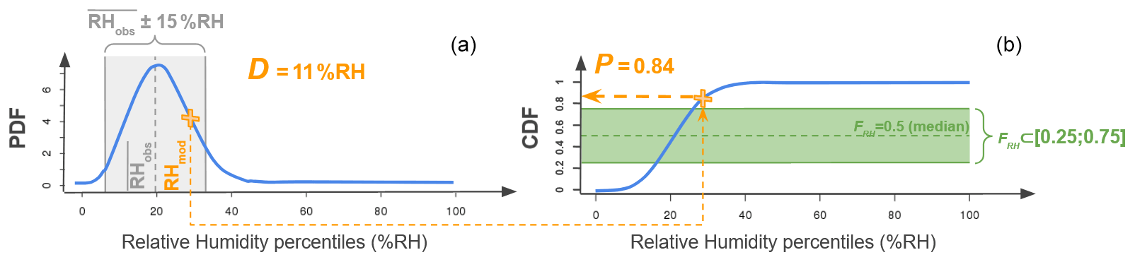
Figure 2Single-grid-box example (grid point situated 24.75 to 25∘ N, 114.5 to 114.75∘ W, and 400–600 hPa for the simulations of 1 April 2018 at 00:00 UTC) showing the projection of RHmod (orange cross) onto its associated reference distribution RHobs (blue curve) in terms of PDF (a) and CDF (noted FRH; b). The reference expectation (first moment of the distribution) noted is drawn as the gray dotted line centered within a ±15 % RH range (gray shade) on the PDF. The expected value (median) of the distribution is shown as the dotted green line on the CDF, and the 0.25–0.75 quantile interval is shaded in green.
The value FRH (RHmod) represents the probability P that RHobs takes on values lower than or equal to the RHmod:
The probability P indicates the position of RHmod within the distribution of RHobs. A probability value P∼0.5 indicates that RHmod is close to the median, which is a representative value of RHobs. A probability value P < 0.1 (> 0.9, respectively) indicates that ARPEGE probably underestimates (overestimates, respectively) the reference RHobs as there is less than a 10 % chance that the RHobs takes on lower (greater, respectively) values.
In order to compare the probabilistic method to a more classic approach, a simple deterministic comparison is used as a benchmark. The mean reference value is calculated as the first moment of the PDF, and it is taken as the reference in the deterministic comparison.
The deterministic bias D is defined as the difference between the RHmod and the mean observed value . A D close to 0 indicates that the RHmod is close to the mean reference . An a priori deterministic ±15 % RH confidence interval (gray shading in Fig. 2a) centered around is chosen to account for uncertainties in the reference. The 15 % RH uncertainty value is the smallest that allows the uncertainties in all pressure layers to be encompassed (see Sect. 2.1 or Brogniez et al., 2016, for a more complete analysis of uncertainty). It is a reasonable value that can be applied to the full RH profile. Note that the retrieval uncertainty is lower in the mid-tropospheric layers compared to the edges of the profiles (Sivira et al., 2015). In terms of deterministic comparison D < −15 % RH (> 15 % RH, respectively) means that RHmod significantly underestimates (overestimates, respectively) the reference average observation as it falls outside its confidence interval.
Compared to a deterministic comparison between ARPEGE's RHmod and the reference , FRH (RHmod) objectively quantifies the significance of the departure of ARPEGE with respect to the reference RHobs central value by factoring in (normalizing by) the spread of the distribution. This allows us to quantify the occurrence of extreme biases from the model while accounting for the tails of the distribution. By accounting for the complete reference distribution (and its characteristics like the spread and asymmetry), this probabilistic formulation allows comparison with greater resolution, sharpness and discrimination than a deterministic comparison at the pixel level.
3.1.2 Application to a single grid box
The deterministic comparison and the CDF-based comparison are applied to each ARPEGE grid point. Figure 2 illustrates further the complementarity of the two approaches for a representative case.
For any given ARPEGE grid box the values P and D are computed from Eqs. (3) and (4). As RHmod rarely falls in a RHobs percentile, P is calculated with a linear interpolation between the two encompassing percentiles. A probabilistic confidence interval for the reference is defined at every ARPEGE grid box as the inter-quartile [0.25, 0.75] (green shading in Fig. 2b). This interval encompasses 50 % of the RHobs distribution centered around the median (FRH= 0.5; dotted green line).
In the example shown in Fig. 2, ARPEGE's RHmod is rather close to the mean reference value as it lies within 15 % RH from (D= 11 % RH; see Fig. 2a). However, the projection of RHmod onto the CDF (Fig. 2b) indicates that it is located in the upper quartile of the distribution outside the [0.25, 0.75] reference confidence interval (Fig. 2b). RHobs has a low probability of P= 0.16 of being lower than or equal to RHmod. In other words, at this grid box and time the probabilistic approach indicates that ARPEGE has a fairly high probability of overestimating RH, while the deterministic comparison indicates an acceptable difference with the averaged value . This example illustrates how the probabilistic comparison increases the information content in the reference by explicitly accounting for the reference uncertainty, which leads to a different conclusion than with the deterministic comparison that is based on a constant a priori uncertainty.
3.2 Applied methodology
3.2.1 Precipitation masking
As underlined in Sect. 2.1, the retrieval of RH profiles from SAPHIR measurements is performed for both clear sky and cloud-covered areas to the extent that scattering by large hydrometeors produced by convective activity is negligible (Greenwald and Christopher, 2002; Hong et al., 2005). Therefore, all ARPEGE grid boxes associated with rainfall rates strictly above 0 mm h−1 are filtered out.
3.2.2 Temporal statistical accumulation
The comparison method is applied to a spatiotemporal domain covering the tropical belt over 3 months (April–May–June 2018). D values are calculated at each grid box and time step and are averaged over time into a value representing the average departure between ARPEGE's RHmod and the reference at this grid box. In terms of the probabilistic comparison, P values are also calculated at each grid box and time step and are aggregated over time to compute a PDF (Kirstetter et al., 2015), whose mode P3M (3M stands for “3 months”) is kept. Figure 3 illustrates this process.
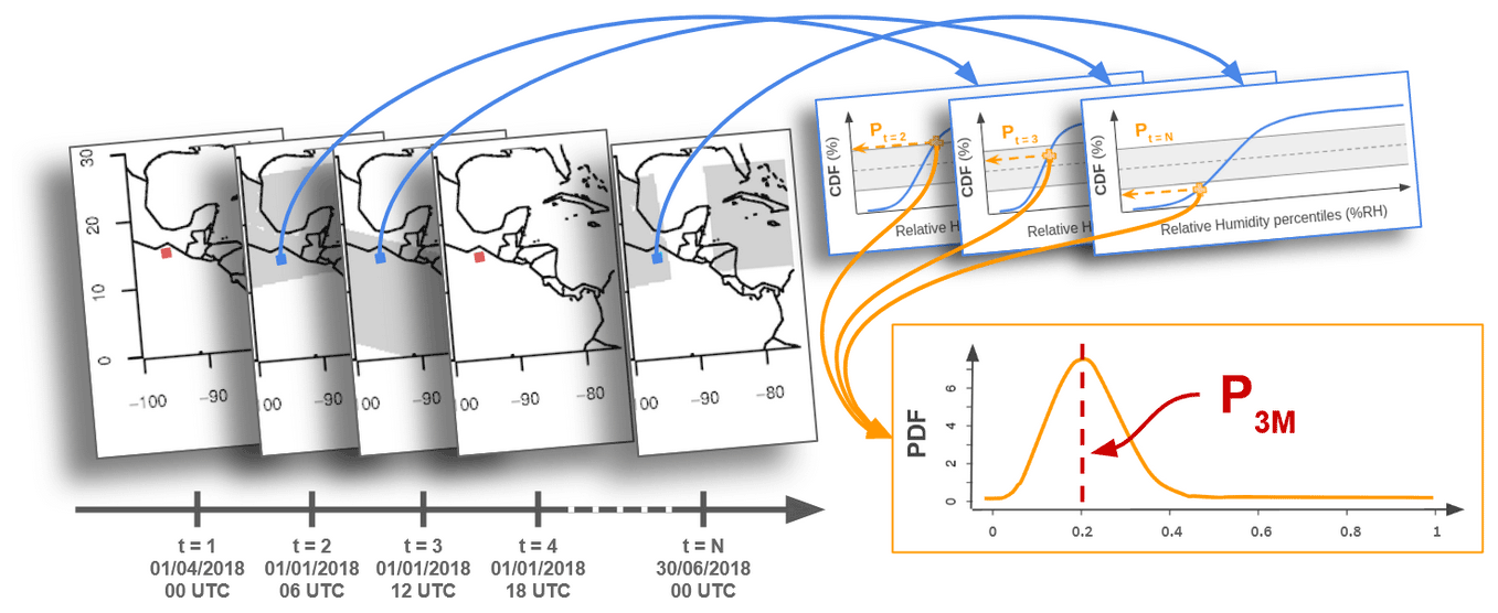
Figure 3Diagram presenting the spatial and temporal aggregation method for a single grid point (blue square when the grid box was passed over by SAPHIR, red when not and/or filtered out). P3M is the mode of the distribution aggregated over all the considered time steps for this grid box.
4.1 Uncertainty related to the assumption of Gaussian distributions
In deterministic comparison settings, the uncertainty may be defined based on a priori assumptions, instrumental biases and retrieval errors. This uncertainty is often assumed to be multiplicative with respect to the reference value, and it is assumed that the underlying density function is unimodal, symmetric and follows a Gaussian model so that the uncertainty is defined as a standard deviation. However, a Gaussian model would not have been adapted to the dataset. A Shapiro–Wilk test is run with each and every individual PDF of the dataset (with αSW= 0.01). The Shapiro–Wilk test is a widely used test of normality in statistics (Shapiro and Wilk, 1965). Finding a p value above αSW would mean that the null hypothesis (“the PDF fits a normal distribution”) cannot be refuted. For each pressure layer, more than 99.99 % of the PDFs have p values under αSW, meaning that almost none of them can be qualified as Gaussian. With the probabilistic approach, the uncertainty can be defined with the inter-quartile range (IQR) of the distribution calculated from the CDF at each time step and each grid box (see Sect. 3.1.2). The IQR represents the difference between the RH values corresponding to probabilities of 0.75 and 0.25. Note that no assumption is made on the shape of the distribution in this case; hence the uncertainty is objectively and robustly quantified.
The smaller the IQR, the narrower the distribution and the smaller the uncertainty in the reference. Values of the IQR can be compared with the deterministic 15 % RH uncertainty. If the IQR is greater (lower, respectively) than 15 % RH, then the reference distribution is broader (narrower, respectively) than assumed with a set 15 % RH error.
Figure 4a and b show an example of reference and the associated IQR calculated at a given time step (1 April 2018 at 00:00 UTC) and for a given atmospheric layer (650–700 hPa). Figure 4c shows the frequency of occurrence for cases with IQR > 15 % RH at each grid box over the 3-month period April–June 2018.
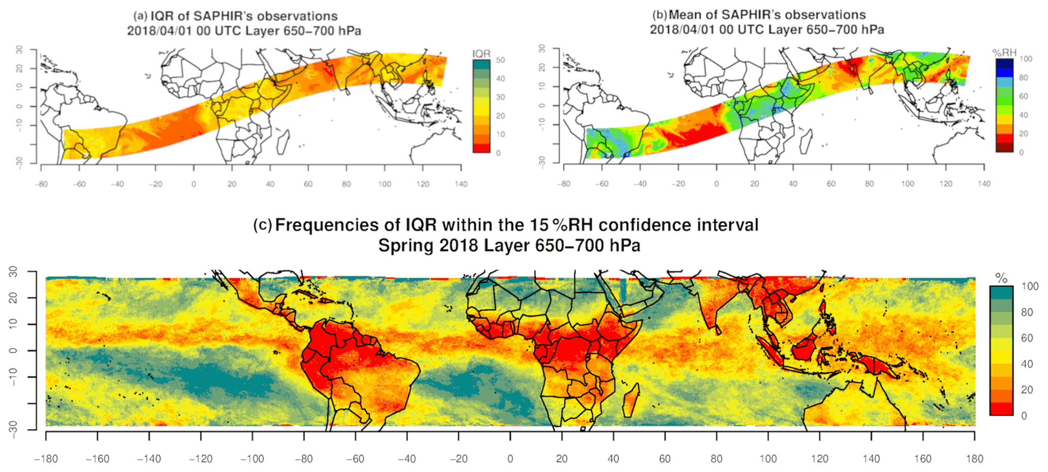
Figure 4(a) Spatial distribution of the inter-quartile range (IQR) and (b) mean of reference ( representing the observed spatial field of RH from SAPHIR on 1 April 2018 at 00:00 UTC and in the 650–700 hPa layer. (c) Frequency of IQR ≤ 15 % RH over the 3-month period (April to June 2018).
The spatial distribution of the IQR (Fig. 4a) shows contrasted areas that match the patterns of (Fig. 4b). Low IQR values (IQR ≤ 15 % RH; appearing in red and orange in Fig. 4a) are consistently found where the atmosphere is dry, for example above the Atlantic Ocean and the Arabian Sea. High IQR values (IQR > 15 % RH; in yellow to green in Fig. 4a) are found in a moister atmosphere, especially above South America, Africa and South Asia. This suggests that while scaling relation between RH and its uncertainty is relevant, a typical 15 % RH assumption lacks dynamics to represent the true uncertainty. The contrasted differences between the IQR < 15 % RH and IQR > 15 % RH areas show that the widths of the RHobs distributions vary significantly and are linked to the same processes. In addition, in the areas with IQR > 15 % RH the wider range of RHobs illustrates the equally wide diversity of underlying situations. These results illustrate the need to use a comparison method that adapts to the range of variability at each grid box. Especially in the areas where the IQR is high, using a deterministic approach solely based on the distribution expectation does not capture the variety and complexity of situations and is thus ill-advised. However, we note that high IQR values found in moister situations may also result from multiple causes such as the aggregation of distinct sub-grid processes or higher retrieval errors (Sivira et al., 2015; Brogniez et al., 2016). Nonetheless, using a probabilistic approach makes any comparison more specific to each situation by avoiding the use of a consistent simplification (i.e., a set confidence intervals) that does not fit the underlying complexity.
The comparison of the two uncertainty approaches over the whole period (Fig. 4c) confirms the spatial correlation between the IQR and the classical patterns of the humidity field. This is particularly visible around the South Pacific and South Atlantic highs, where the proportion of IQR under the 15 % RH threshold reaches 70 % and even 100 %. In these subsiding areas, the atmospheric RH is ruled by large-scale processes that have little to no instantaneous variability at the scale of our grid. This results in more homogeneous conditions within the same grid box, which explains the narrower distributions of the retrievals (i.e., smaller IQR). The Intertropical Convergence Zone (ITCZ) appears through areas of low proportion (0 % to 30 % of the retrievals' dataset) of under 15 % RH IQR. High dynamics characterizing this zone result in smaller-scale processes that impact the RH field and result in heterogeneous conditions within the same grid box and larger IQR. Most importantly, IQR varies across space and time, and it can be partly linked to the RH field and explained by large- and fine-scale processes. These highlight the need for a comparison method that exploits and takes into consideration the variability in the dataset and adapts the comparison to each situation.
One can note that while these results vary significantly depending on the atmospheric layer, they are coherent with the expected RH field patterns. For example, in the upper two atmospheric layers (100–200 and 250–350 hPa), the homogeneous dryer conditions result in almost all retrieval distributions having IQR under 15 % RH. The two lower layers (750–800 and 850–950 hPa), closer to the ground, show strong ocean–continent contrasts. This contrast shows the difference in processes that depend on the surface, with extremely low frequencies of IQR under 15 % RH above the continents. This suggests that the lower the layer, the wider the distribution of retrieved RH.
In all cases where the IQR is above 15 % RH, flattened and possibly non-Gaussian RH distributions may result in non-representative values associated with varying confidence intervals that make the deterministic comparison less appropriate. These results show that these situations can be quite frequent and geographically distributed. The probabilistic method allows us to adapt the confidence to each distribution regardless of the width and shape and thus improves the assessment accuracy both overall and at the grid box and time step scale.
4.2 Application to a single time step
Figure 5 shows the comparison results between the reference RHobs and ARPEGE's RHmod obtained with both deterministic and probabilistic methods.

Figure 5Comparisons between SAPHIR's and ARPEGE's RHmod on 1 April 2018 at 00:00 UTC and for the 400–600 hPa atmospheric layer. (a) Map of the difference D, (b) map of the probability P, and (c) scatterplot between (x axis) and RHmod (y axis); the percentile associated with each point is P > 0.75 (blue), 0.25 < P < 0.75 (gray) and P < 0.25 (red); the solid line represents the y=x line, and the dotted lines delimit the ± 15 % RH around values.
The comparisons are performed using wide discrete color bars in order to discuss the complementarity of the methods and not specific issues of the model. The deterministic approach shows that a majority of RHmod values are within the interval of ±15 % RH of (gray areas in Fig. 5a). By contrast, the probabilistic approach reveals that only a few of the corresponding P values fall within the [0.25, 0.75] probabilistic interval (blue or red in Fig. 5b). Large areas of deterministic reasonable differences such as in the southern Atlantic are associated with P > 0.75, meaning that the corresponding RHmod has a high probability of overestimating the reference. The inset in the maps is a zoom that highlights similar bias patterns with both methods but with higher contrasts with the probabilistic one. The patterns only appear in the deterministic results when using a continuous color scale that allows small differences to be shown with respect to the mean . These patterns can be observed with both methods in general, but the small differences between the RHmod and prevent a robust diagnosis. The probabilistic results are particularly contrasted in comparison because these RHmod values fall into the extreme quartiles (P < 0.25 or P > 0.75). The scatterplot (Fig. 5c) further illustrates the added value of the probabilistic approach. The confidence interval set by P within [0.25, 0.75] (gray triangular shape) closely follows the RH line, showing the overall consistency of the two methods. For small values of RH, this interval is much tighter around the line than at higher values. The confidence interval widens for higher values of RH, confirming that the probabilistic method is more specific than a deterministic approach with constant error bars around the RH line. Furthermore, situations where P falls within the [0.25, 0.75] interval are less common when compared to the ±15 % RH range defined around the mean. The blue and red dots that appear within the ±15 % RH range indicate cases where RHmod is close to (D within [−15, 15]) but falls in extreme RHobs distribution quartiles (P outside [0.25, 0.75]). Most blue and red points (respectively above and under the ±15 % RH range) show that a strong deviation from mean nearly always matches with extremes of the distribution (P < 0.25 or P > 0.75).
In short, the probabilistic method is consistent with the deterministic comparison on extreme biases and adds more information for cases where RHmod seems close to .
4.3 Comparison results for an extended period of time
4.3.1 Distributions
The two methods are applied to the entire dataset over the period from April to June 2018. The distributions of each method's results are represented as a histogram (Fig. 6a) and rank histogram diagram, also known as a Talagrand diagram (Hamill, 2001; Wilks, 2011; Kirstetter et al., 2015; Fig. 6b). Note that while the Talagrand diagram is often used to assess ensemble forecasts by comparing a single reference to a distribution of forecast ensembles, its interpretation is similar when comparing a single simulated value to a reference distribution. This graphical method illustrates where the ARPEGE's RHmod falls in the distribution function CDF of RHobs. In the case of perfect forecasts, each quantile represents an equally likely scenario for the ARPEGE model. The perfect case is a flat rank histogram indicating that the RHobs probability distribution is well represented by RHmod.
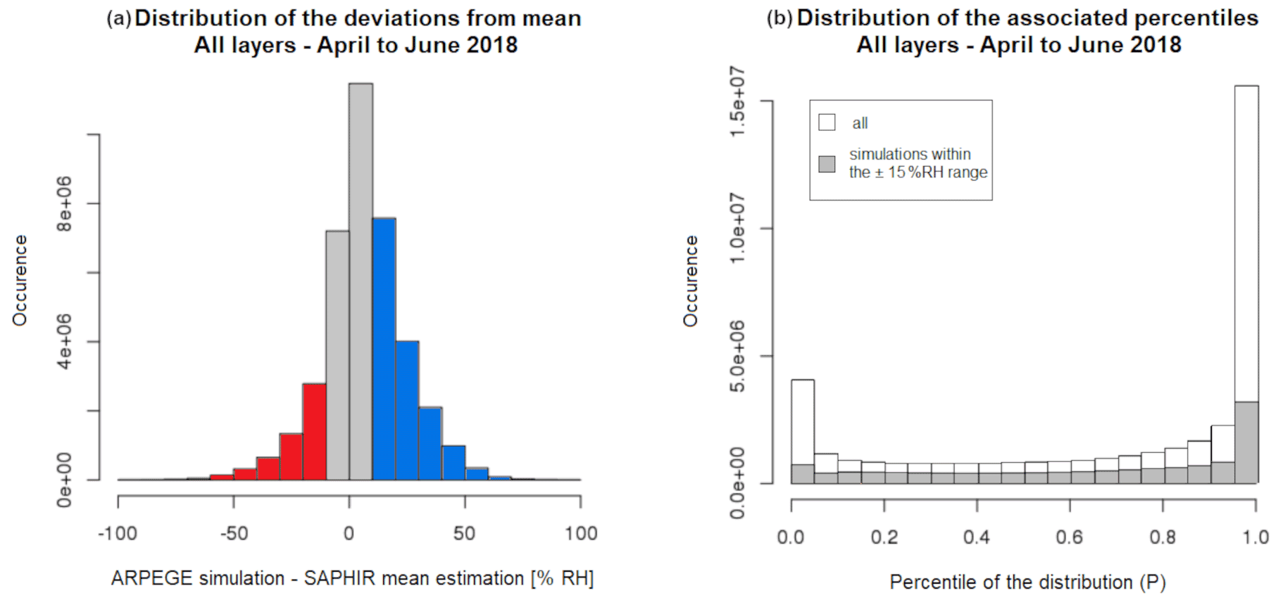
Figure 6Distribution of the results from each comparison method applied to all layers over the period April to June 2018: (a) histogram of the deviations D from the mean (in red: D < −15 % RH; gray: −15 % RH 15 % RH; blue: D > 15 % RH) and (b) rank histogram diagram, also known as a Talagrand, of P (in gray: values of P when D is within [−15, 15] % RH; in white: for all values of D).
As seen in Fig. 6a, the deterministic difference D= RHmod− displays a unimodal and symmetrical distribution centered around 0. All layers combined, more than 67 % of the RHmod values deviate by less than 15 % RH from the mean estimate . Nearly 20 % of all RHmod values are too high by more than 15 % RH and fewer than 2 % by more than 50 % RH. Yet the Talagrand diagram in Fig. 6b shows that the associated percentiles P display a bimodal distribution with maximum frequencies concentrated at the two extreme ends. Half the ARPEGE's RHmod values are associated with extreme percentiles of the RHobs distribution (P < 0.05 or P > 0.95). Fewer than a quarter (23.3 %) of the RHmod values fall within the centered half of the RHobs distribution. The Talagrand diagram allows us to draw direct conclusions on the reliability of the forecasts. Assuming that the forecasts are spread far enough in both time and space to be considered independent from each other, the probabilities of finding each percentile of the histogram should be fairly equal, giving the diagram a flattened aspect, which is not observed here. The U shape indicates that the extreme classes are over-represented and compensate for the underestimations of the central quantiles (Candille and Talagrand, 2005). There is also a tendency of ARPEGE to overestimate RH. These features remain when focusing on RHmod values within the 15 % RH from the mean estimate (gray histogram in Fig. 6b). This confirms that the overestimation is present within the deterministic confidence range. Validating RHmod values by their proximity to the mean reference (−15 < D < +15 % RH) is not sufficient to assess their accuracy, especially when they fall in the extreme percentiles of the associated distribution (P < 0.25 or P > 0.75).
The comparisons are performed independently for each atmospheric layer in Fig. 7. The distributions are represented as boxplots in Fig. 7, with the width of the box defined by the first and third quartiles, and the whiskers indicate the most extreme values but with their length limited to 1.5× IQR. This highlights a variability in terms of both shift and spread.
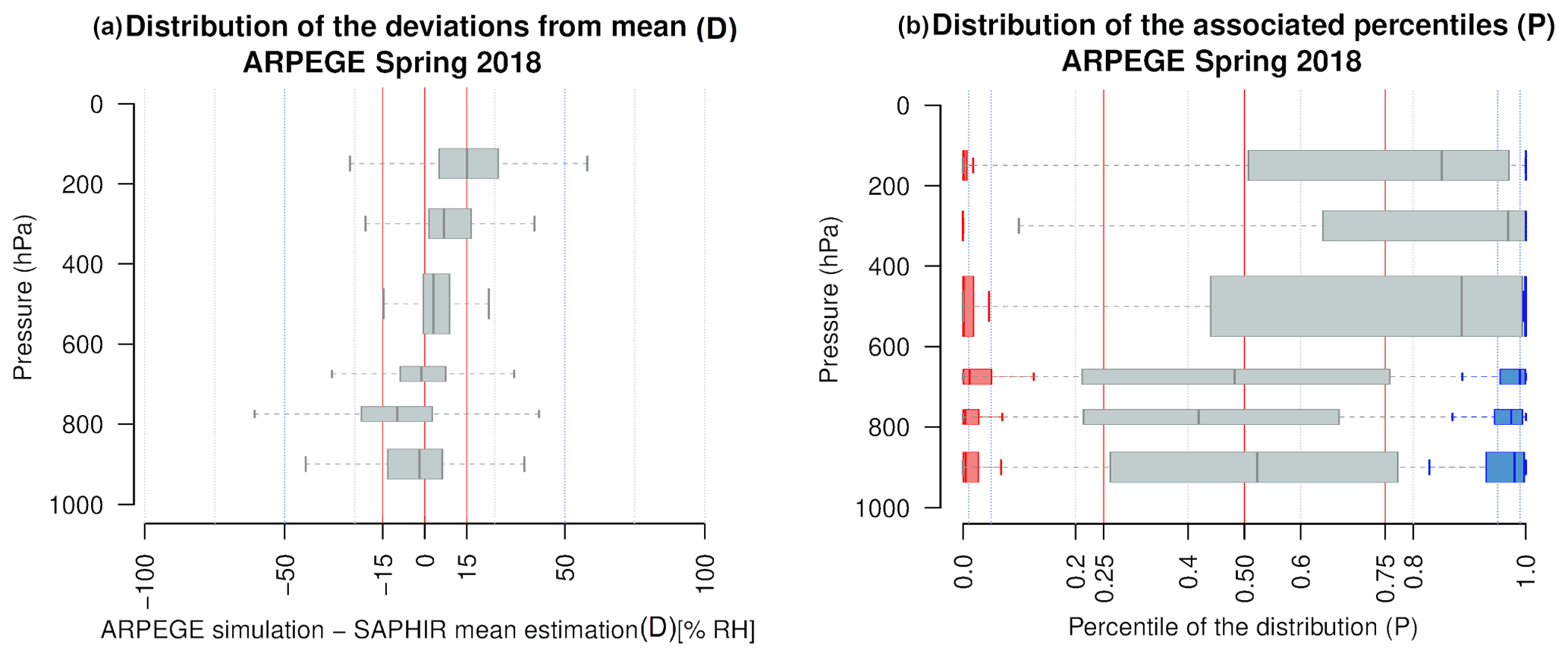
Figure 7Distribution the results of each method of comparison applied over the period April to June 2018 represented as boxplots for each layer: (a) deviations D from mean and (b) associated percentiles P divided into three distribution types depending on the category of D (red: D < −15 % RH; gray: −15 % RH 15 % RH; blue: D > 15 % RH). The weights of each category within their layer's distribution are indicated in Table 1.
The distributions of the deviations from the mean D (Fig. 7a) show a tendency of the model to overestimate in the upper-tropospheric layers (100–200, 250–350 hPa), to close in on in the mid-tropospheric layers (400–600 hPa) and to slightly underestimate in the lower-tropospheric layers (650–950 hPa). The highest layer (100–200 hPa) has the most off-centered results, with half (50.3 %) of the simulated values overestimating by more than 15 % RH. More than a third (38.7 %) of the simulations in the layer 750–800 hPa are more than 15 % RH below (D < −15 % RH). The other layers have the majority of their distribution well within the ±15 % RH range.
The distributions of the associated percentiles are wider (Fig. 7b) and offer a deeper understanding. The comparison results are divided into three categories that follow the deviation from the mean intervals. They are drawn separately to highlight the consistency of the two methods' extreme results. The ARPEGE's RHmod values distant from by more than 15 % RH (D outside [−15, 15]) almost always fall in either one or the other extreme end of the estimated distribution (red and blue boxplots in Fig. 7b). Table 1 provides, for each atmospheric layer, the portion of the distributions that fall inside or outside the interval [−15%; 15 %]. The proportion of extremes varies from one layer to the another. This allows us to separate the two maxima of the U shape of the rank histogram (Talagrand) diagram (Fig. 6b): the left-hand extreme is largely influenced by the underestimated values in the lower layers (750–800, 850–950 hPa), while the right-hand extreme is driven by the over-representation of overestimations in the higher layers (100–200, 250–350 hPa).
Table 1Part (in percent) of the distributions within the three categories of differences D for each atmospheric layer.
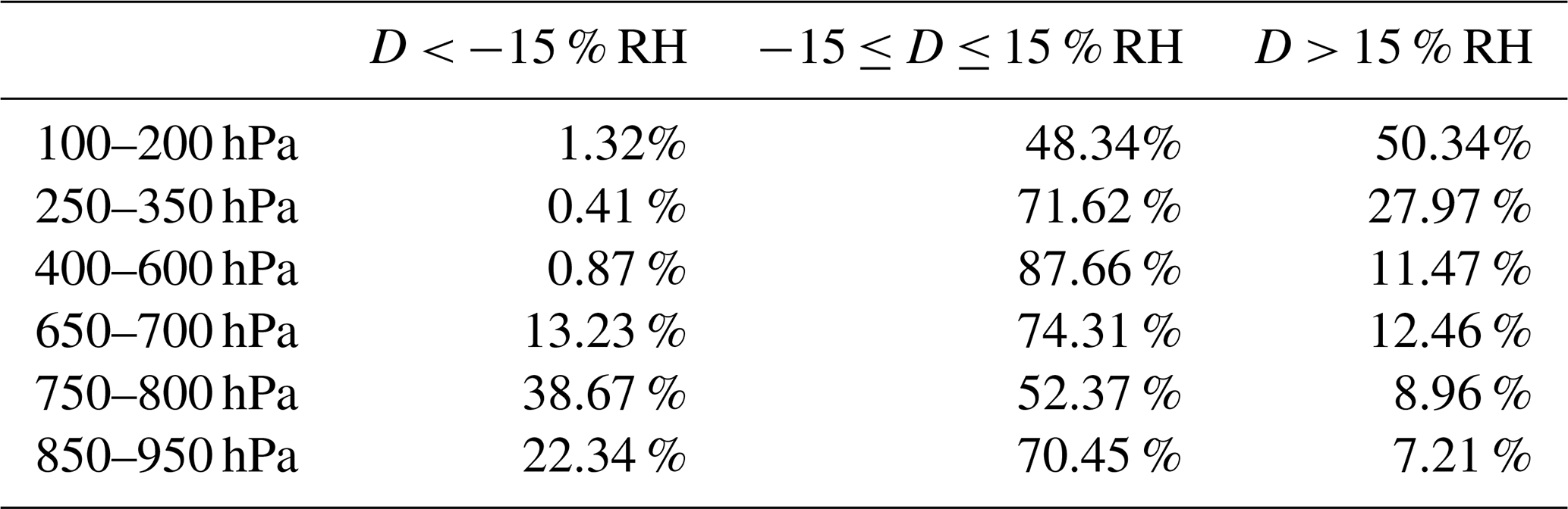
An added value of the probabilistic approach resides in the contrast and variability in the results within the ±15 % RH range. As previously shown, the implicit hypothesis in a deterministic method does not allow the confidence interval to be narrowed further than 15 % RH, thus preventing a more contrasted diagnosis of the model's outputs. The gray boxplots highlight the great variability in cases contained within the deterministic interval that is not revealed by a small difference D to the mean estimate . Even though the distributions of P are fairly spread, in the highest layers (above 400 hPa) they have a strong tendency to fall in higher percentiles of the reference distributions: more than 75 % of the simulations of the first two layers (between 100 and 350 hPa) are above 0.75 % and 65 % into the upper 0.05. This confirms the general overestimation displayed by the deterministic results in these layers. The underestimations of the lower layers are also clear, with 54.4 % and 39.1 % of the simulations falling into the lower quarter of the reference distribution in the second-to-lowest layer (750–800 hPa) and lowest layer (850–950 hPa), respectively. The distribution of the 650–700 hPa layer is the most centered, yet it is spread and still has more than half of the associated percentiles (66.2 %) outside the 0.25–0.75 interval.
The 400–600 hPa layer has the narrowest distribution of deviations from the mean within the ±15 % RH range. However, the distribution of the associated percentiles is mostly located towards the higher half (64.7 % above 0.75), and nearly half of the simulations (47.0 %) fall into the upper extreme 0.05 %.
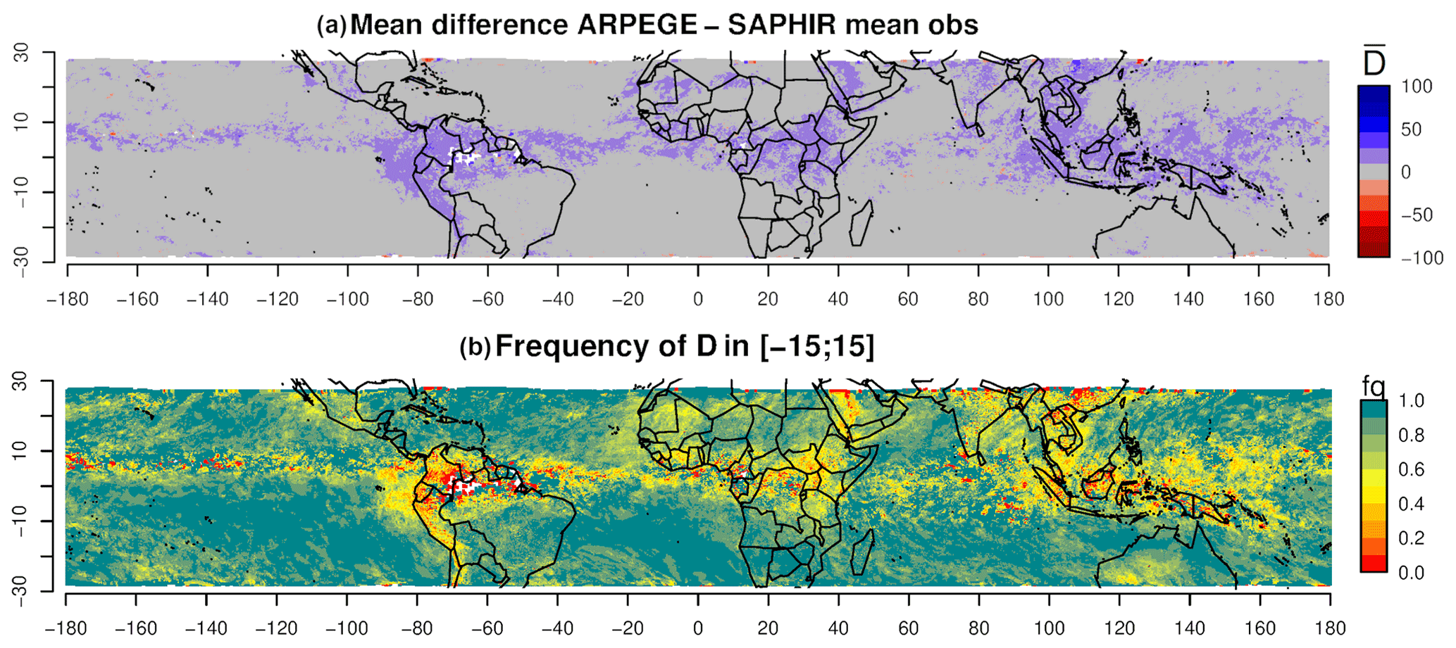
Figure 8Deterministic comparisons for layer 400–600 hPa over the period from April to June 2018. (a) Map of the mean difference and (b) frequency of instantaneous difference D falling within [−15, 15] over the 3-month period.
4.3.2 Maps: deterministic results
The two maps in Fig. 8 show the results of the deterministic approach in terms of the average deviation from ( (Fig. 8a) and frequency of RHmod within the ±15 % RH range (Fig. 8b) for the 400–600 hPa layer (other layers can be found in the Supplement). The combined results of the 3-month period show recognizable patterns.
The majority of the average deviations are close to zero (displayed in gray in Fig. 8a). These regions have 80 % to 100 % of single-time-step D within the ±15 % RH range (light to dark green in Fig. 8b). On average, the model's overestimated RH values (blue) are localized above known convective areas (ITCZ, South Pacific Convergence Zone, orographic convection areas along the western coast of South America). These on-average overestimated zones are characterized by low frequencies of single-time-step D within the ±15 % RH range (50 % and less, appearing as yellow and orange in Fig. 8b). This indicates that this potential bias occurs at least half the time over the study period. Only a small number of pixels show an on-average underestimation (red), as predicted by the distribution of the deviation results (see Fig. 7a and the discussion in Sect. 4.3.1).
The results of this method reveal a slight moist bias in the convective zones but mostly validate ARPEGE simulations everywhere else outside these areas.
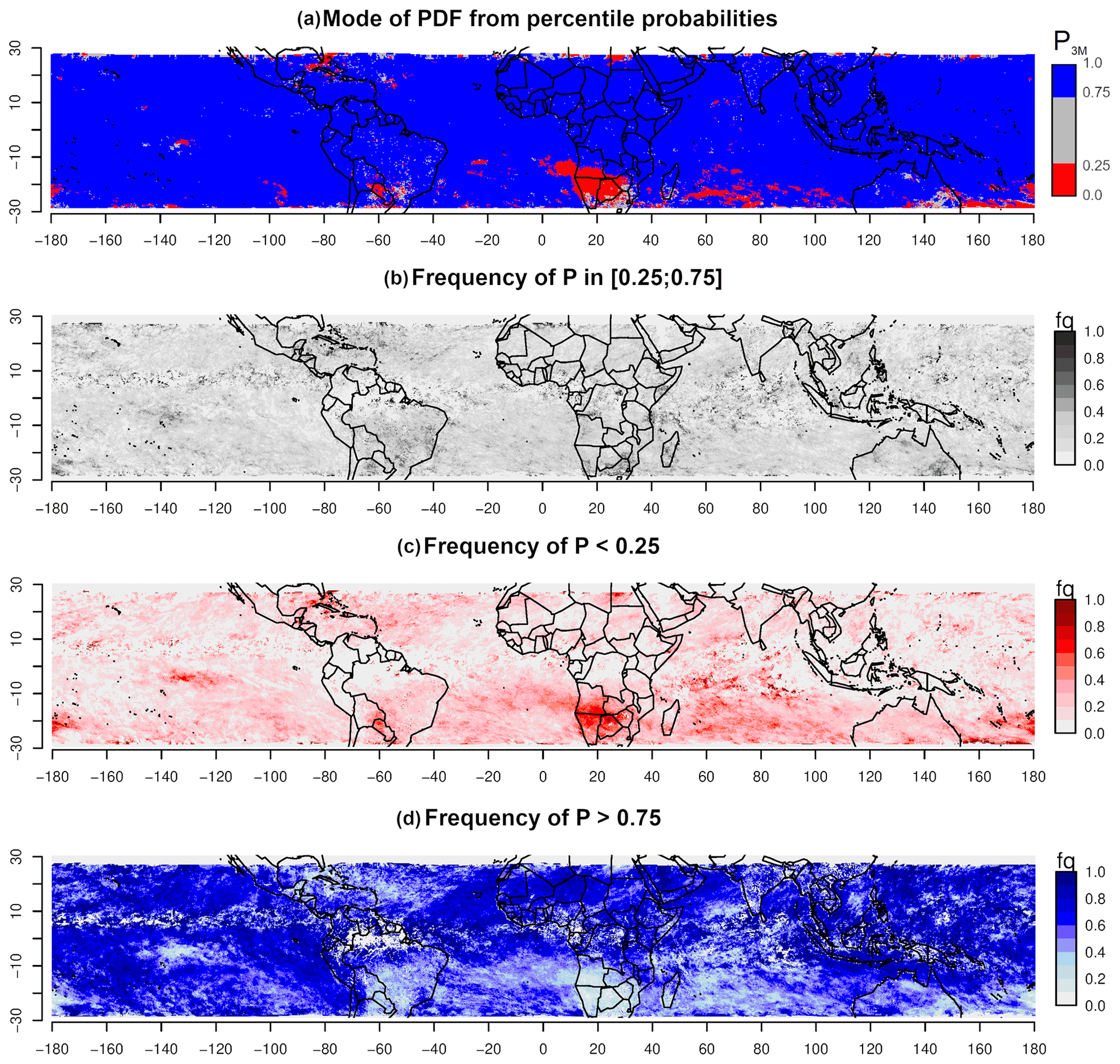
Figure 9Maps of the probabilistic method for the layer 400–600 hPa applied over the period from April to June 2018. (a) Mode P3M and frequencies of single-time-step P within (b) the middle half (0.25 0.75), (c) lower quarter (P < 0.25) and (d) upper quarter (P > 0.75) of the distribution of estimates.
4.3.3 Maps: probabilistic results
Figure 9 represents maps of the probabilistic comparison method in terms of spatial distribution of the mode P3M of the PDF calculated from the single-time-step P aggregated over the 3 months and the frequencies of P within the three categories (P < 0.25, 0.25 0.75, P > 0.75).
The probabilistic comparison method highlights a majority of contrasted extreme values, which indicates a high probability of ARPEGE's RHmod falling into one or the other extreme quarter of the RHobs CDF. The maps show organized and contrasted spatial patterns with a majority of overestimated areas (blue to dark blue in Fig. 8a) along with some underestimated patches (red to dark red). The overestimations are predominant with a frequency of at least 40 % in most areas (Fig. 8d). The convective zones are overestimated with the deterministic method but seem more complex, with probability P falling in both the middle half and the upper extreme segments of the RHobs CDF.
The red patch located south of the African continent (Fig. 9a) indicates a recurring underestimation of the model, with RHmod values falling in the lower quarter of the RHobs CDF. These underestimations happen at least half of the time during the studied period (in bright red in Fig. 9c). The frequencies of simulated values within the middle-half part of the reference distribution are fairly low (mostly under 0.4; Fig. 9b). The frequencies of P > 0.75 are almost null (Fig. 9d). Other underestimated areas can be observed, e.g., above the Caribbean and above the Pacific Ocean, east of Australia. Above the Indian Ocean, even though most D values are within the ±15 % RH range, the situation appears to be significantly more contrasted with the probabilistic approach. Again, the deterministic approach only finds RHmod values close to ; the probabilistic method assigns high probabilities for RHmod to fall into one or the other extreme of the RHobs distribution. In this area, both high frequencies of P in the lower and the upper quarters of the distribution are found spatially close to each other and without any particular pattern (speckled aspect in the Indian Ocean; Fig. 9a, c and d).
These various problematic areas do not particularly stand out when solely using a deterministic comparison approach. The probabilistic method allows for a more contrasted and detailed assessment. Note that the analysis of the results with regard to the model specificities, such as its parameterization of convection, are outside the scope of this paper.
This paper showcases the importance of considering all the reference information content through a probabilistic approach that considers the reference distribution to assess ARPEGE model simulations. The probabilistic reference is derived from finer-scale RH estimates aggregated into a probability density function at the ARPEGE spatial resolution. In widely used deterministic comparison approaches, the reference distribution is only considered through its first moment (and sometimes its second moment). Moreover, nowadays, a lot of satellite products offer a second moment that enables intercomparison studies. However, the propagation of uncertainties assumes a Gaussian distribution, which is not the case here. We developed a probabilistic approach for the retrieval of RH that gets rid of such assumptions.
The improved assessment with the probabilistic approach is demonstrated by comparing the insights obtained on ARPEGE with those from a deterministic method involving the difference and a ±15 % RH confidence interval.
Initial results highlight the inherent inaccuracy of solely using averaged references due to the important variability in spread and shape of the reference estimates. By computing the inter-quartile range (IQR) for the whole reference dataset, it was found that the spread of the PDFs varies significantly and is linked to the RH magnitude, with wider distributions in moist areas and narrower distributions in drier conditions. A deterministically set confidence interval is relevant to the variability in the spread to some extent only. This promotes a comparison method that quantifies more precisely the deviation of the simulated value irrespective of the reference distribution variability, spread and shape.
Both deterministic and probabilistic methods were confronted in a single time step and over the 3-month period. Most RH values simulated by ARPEGE fit within the ±15 % RH confidence interval with a slight moist bias detected in the ITCZ. However, the probabilistic method reveals that RHmod values that differ from by more than 15 % RH (D < −15 % RH or D > +15 % RH) often correspond to the extreme 5 % of the reference distributions (P < 0.5 or P > 0.95). The probabilities associated with RHmod values within the deterministic confidence range are often outside the probabilistic confidence interval [0.25, 0.75], which highlights model biases. The highest layers (100–600 hPa) show high occurrence of probabilities within the upper quartile of the reference distributions (P > 0.75), allowing the conclusion that ARPEGE overestimates RH in these layers. The middle and lower layers (600–950 hPa) have P distributions more centered around the reference median but that are wider than the 0.25–0.75 interval. For these layers, the spatial distribution of the probabilistic results shows a likely overestimation of ARPEGE in convective areas and a tendency to underestimate specific subsiding systems. This last observation is not detected with the deterministic method, and it adds new perspectives on potential biases of ARPEGE.
Overall, the probabilistic comparison allows a more contrasted and complete assessment. The bias structures that are revealed fit known humidity patterns. A more complete analysis with regard to the model's specificities could help highlight areas of improvement. The method presented here can be generalized to different models, variables and observations.
The underlying codes were developed for research and are not suited for direct implementation. Their specificities may be shared and/or discussed upon request from the author and acknowledged colleagues.
SAPHIR data are available through the AERIS/ICARE ground segment of Megha-Tropiques (https://www.icare.univ-lille.fr/product-documentation/?product=SAPHIR-L2B-RH, Sivira et al., 2022). More information on the dataset can be found in Sivira et al. (2015) and Brogniez et al. (2016). Both papers are already listed in the references section. ARPEGE data could be made available upon request.
The supplement related to this article is available online at: https://doi.org/10.5194/acp-22-3811-2022-supplement.
The present work is the result of an original idea of HB and PEK, developed by CR under the supervision of HB, PEK and PC. HB provided and added her expertise on the SAPHIR dataset, PC on the ARPEGE dataset and PEK on the statistical method itself. All authors discussed the results and contributed to the final paper.
The contact author has declared that neither they nor their co-authors have any competing interests.
Publisher's note: Copernicus Publications remains neutral with regard to jurisdictional claims in published maps and institutional affiliations.
This article is part of the special issue “Analysis of atmospheric water vapour observations and their uncertainties for climate applications (ACP/AMT/ESSD/HESS inter-journal SI)”. It is not associated with a conference.
We thank the CNES for its financial support through the Megha-Tropiques project and the national AERIS data center, which hosts the satellite data. Christophe Dufour (LATMOS/IPSL) contributed to the data processing. Computing resources of the ESPRI IPSL mesocenter were greatly appreciated. Pierre Kirstetter acknowledges support from the NASA Global Precipitation Measurement Ground Validation program under grant NNX16AL23G. We would also like to thank Joern Ungermann and the anonymous referee, whose insightful comments helped us convey our work in the clearest way.
Financial support was partly brought by the CNES French Space Agency through the Megha-Tropiques project.
This paper was edited by Martina Krämer and reviewed by Joern Ungermann and one anonymous referee.
Aires, F., Rossow, W. B., Scott, N. A., and Chedin, A.: Remote sensing from the infrared atmospheric sounding interferometer instrument, 2, Simultaneous retrieval of temperature, water vapor, and ozone atmospheric profiles, J. Geophys. Res., 107, 4620, https://doi.org/10.1029/2001JD001591, 2002.
Allan, R. P.: The Role of Water Vapour in Earth's Energy Flows, Surv. Geophys., 33, 557–564, https://doi.org/10.1007/s10712-011-9157-8, 2012.
Bodas-Salcedo, A., Webb, M. J., Bony, S., Chepfer, H., Dufresne, J.-L., Klein, S. A., Zhang, Y., Marchand, R., Haynes, J. M., Pincus, R., and John, V. O.: COSP: Satellite simulation software for model assessment, B. Am. Meteorol. Soc., 92, 1023–1043, https://doi.org/10.1175/2011BAMS2856.1, 2011.
Bony, S., Stevens, B., Frierson, D. M. W., Jakob, C., Kageyama, M., Pincus, R., Shepherd, T. G., Sherwood, S. C., Siebesma, A. P., Sobel, A. H., Watanabe, M., and Webb, M. J.: Clouds, circulation and climate sensitivity, Nat. Geosci., 8, 261–268, https://doi.org/10.1038/ngeo2398, 2015.
Bouyssel, F., Bazile, E., Piriou, J.-M., Janisková, M., and Bouteloup, Y.: L'évolution opérationnelle du modèle Arpège et de ses paramétrisations physiques, La Météorologie, 112, 47–54, 2021.
Brogniez, H., Roca, R., and Picon, L.: Evaluation of the distribution of subtropical free tropospheric humidity in AMIP-2 simulations using METEOSAT water vapor channel data, Geophys. Res. Lett., 32, L19708, https://doi.org/10.1029/2005GL024341, 2005.
Brogniez, H., Kirstetter, P.-E., and Eymard, L.: Expected improvements in the atmospheric humidity profile retrieval using the Megha-Tropiques microwave payload, Q. J. Roy. Meteor. Soc., 139, 842–851, https://doi.org/10.1002/qj.1869, 2013.
Brogniez, H., Fallourd, R., Mallet, C., Sivira, R., and Dufour, C.: Estimating Confidence Intervals around Relative Humidity Profiles from Satellite Observations: Application to the SAPHIR Sounder, J. Atmos. Ocean Tech., 33, 1005–1022, https://doi.org/10.1175/JTECH-D-15-0237.1, 2016.
Candille, G. and Talagrand, O.: Evaluation of probabilistic prediction systems for a scalar variable, Q. J. Roy. Meteor. Soc., 131, 2131–2150, https://doi.org/10.1256/qj.04.71, 2005.
Chambon, P., Zhang, S. Q., Hou, A. Y., Zupanski, M., and Cheung, S.: Assessing the impact of pre-GPM microwave precipitation observations in the Goddard WRF ensemble data assimilation system: Impact of Pre-GPM Microwave Precipitation Observations, Q. J. Roy. Meteor. Soc., 140, 1219–1235, https://doi.org/10.1002/qj.2215, 2014.
Chepfer, H., Bony, S., Winker, D., Chiriaco, M., Dufresne, J.-L., and Sèze, G.: Use of CALIPSO lidar observations to evaluate the cloudiness simulated by a climate model, Geophys. Res. Lett., 35, L15704, https://doi.org/10.1029/2008GL034207, 2008.
Courtier, P., Freydier, C., Geleyn, J. F., Rabier, F., and Rochas, M.: The ARPEGE project at METEO-FRANCE, ECMWF Seminar on Numerical Methods in Atmospheric Models, Reading, England, 9–13 September 1991, https://www.ecmwf.int/en/elibrary/8798-arpege-project-meteo-france (last access: 18 March 2022), 1991.
Desbois, M., Capderou, M., Eymard, L., Roca, R., Viltard, N., Viollier, M., and Karouche, N.: Megha-Tropiques: un satellite hydrométéorologique franco-indien, La Météorologie, 57, 19–27, https://doi.org/10.4267/2042/18185, 2007.
Geer, A. J. and Baordo, F.: Improved scattering radiative transfer for frozen hydrometeors at microwave frequencies, Atmos. Meas. Tech., 7, 1839–1860, https://doi.org/10.5194/amt-7-1839-2014, 2014.
Greenwald, T. J. and Christopher, S. A.: Effect of cold clouds on satellite measurements near 183 GHz, J. Geophys. Res., 107, 4170, https://doi.org/10.1029/2000JD000258, 2002.
Hamill, T. M.: Interpretation of Rank Histograms for Verifying Ensemble Forecasts, Mon. Weather Rev., 129, 550–560, https://doi.org/10.1175/1520-0493(2001)129<0550:IORHFV>2.0.CO;2, 2001.
Hartmann, D. L., Tank, A. M. G. K., Rusticucci, M., Alexander, L. V., Brönnimann, S., Charabi, Y. A. R., Dentener, F. J., Dlugokencky, E. J., Easterling, D. R., Kaplan, A., Soden, B. J., Thorne, P. W., Wild, M., and Zhai, P.: Observations: Atmosphere and surface, in: Climate Change 2013 – The Physical Science Basis: Working Group I Contribution to the Fifth Assessment Report of the Intergovernmental Panel on Climate Change, Cambridge University Press, Cambridge, 159–254, https://doi.org/10.1017/CBO9781107415324.008, 2013.
Held, I. M. and Soden, B. J.: Water Vapor Feedback and Global Warming, Annu. Rev. Energ. Env., 25, 441–475, https://doi.org/10.1146/annurev.energy.25.1.441, 2000.
Hong, G.: Detection of tropical deep convective clouds from AMSU-B water vapor channels measurements, J. Geophys. Res., 110, D05205, https://doi.org/10.1029/2004JD004949, 2005.
Jiang, J. H., Su, H., Zhai, C., Perun, V. S., Genio, A. D., Nazarenko, L. S., Donner, L. J., Horowitz, L., Seman, C., Cole, J., Gettelman, A., Ringer, M. A., Rotstayn, L., Jeffrey, S., Wu, T., Brient, F., Dufresne, J.-L., Kawai, H., Koshiro, T., Watanabe, M., LÉcuyer, T. S., Volodin, E. M., Iversen, T., Drange, H., Mesquita, M. D. S., Read, W. G., Waters, J. W., Tian, B., Teixeira, J., and Stephens, G. L.: Evaluation of cloud and water vapor simulations in CMIP5 climate models using NASA “A-Train” satellite observations, J. Geophys. Res.-Atmos., 117, D14105, https://doi.org/10.1029/2011JD017237, 2012.
John, V. O. and Soden, B. J.: Does convectively-detrained cloud ice enhance water vapor feedback?, Geophys. Res. Lett., 33, L20701, https://doi.org/10.1029/2006GL027260, 2006.
Karbou, F., Aires, F., Prigent, C., and Eymard, L.: Potential of Advanced Microwaves Sounding Unit-A (AMSU-A) and AMSU-B measurements for atmospheric temperature and humidity profiling over land, J. Geophys. Res., 110, D07109, https://doi.org/10.1029/2004JD005318, 2005.
Kirstetter, P. E., Gourley, J. J., Hong, Y., Zhang, J., Moazamigoodarzi, S., Langston, C., and Arthur, A.: Probabilistic Precipitation Rate Estimates with Ground-based Radar Networks, Water Resour. Res., 51, 1422–1442, https://doi.org/10.1002/2014WR015672, 2015.
Kirstetter, P.-E., Petersen, W. A., Kummerow, C. D., and Wolff, D. B.: Integrated multi-satellite evaluation for the Global Precipitation Measurement mission: Impact of precipitation types on spaceborne precipitation estimation, in: Satellite Precipitation Measurement, chap. 31, edited by: Levizzani, V., Kidd, C., Kirschbaum, D. B., Kummerow, C., Nakamura, K., Turk, F. J., Advances in Global Change Research, 69, Springer-Nature, Cham, 583–608, https://doi.org/10.1007/978-3-030-35798-6_7, 2020.
Morcrette, J.-J.: Radiation and cloud radiative properties in the European Centre for Medium Range Weather Forecasts forecasting system, J. Geophys. Res.-Atmos., 96, 9121–9132, https://doi.org/10.1029/89JD01597, 1991.
Pierrehumbert, R. T.: Infrared Radiation and Planetary Temperature, AIP Conf. Proc., 1401, 232–244, https://doi.org/10.1063/1.3653855, 2011.
Randall, D. A., Wood, R. A., Bony, S., Colman, R., Fichefet, T., Fyfe, J., Kattsov, V., Pitman, A., Shukla, J., Srinivasan, J., Stouffer, R. J., Sumi, A., and Taylor, K. E.: Cilmate Models and Their Evaluation. In:Climate Change 2007: The Physical Science Basis. Contribution of Working Group I to the Fourth Assessment Report of the Intergovernmental Panel on Climate Change, edited by: Solomon, S., Qin, D., Manning, M., Chen, Z., Marquis, M., Averyt, K. B., Tignor, M., and Miller, H. L., Cambridge University Press, Cambridge, United Kingdom and New York, NY, USA, 2007.
Roca, R., Brogniez, H., Chambon, P., Chomette, O., Cloché, S., Gosset, M. E., Mahfouf, J.-F., Raberanto, P., and Viltard, N.: The Megha-Tropiques mission: a review after three years in orbit, Front. Earth Sci., 3, https://doi.org/10.3389/feart.2015.00017, 2015.
Rodgers, C. D. and Connor, B. J.: Intercomparison of remote sounding instruments, J. Geophys. Res., 108, 4116, https://doi.org/10.1029/2002JD002299, 2003.
Rosenkranz, P.: Retrieval of temperature andmoisture profiles from AMSU-A and AMSU-B measurements, IEEE T. Geosci. Remote, 39, 2429–2435, 2001.
Roy, R. J., Lebsock, M., Millán, L., and Cooper, K. B.: Validation of a G-Band Differential Absorption Cloud Radar for Humidity Remote Sensing, J Atmos. Ocean Tech., 37, 1085–1102, https://doi.org/10.1175/JTECH-D-19-0122.1, 2020.
Shapiro, S. S. and Wilk, M. B.: An Analysis of Variance Test for Normality (Complete Samples), Biometrika, 52, 591–611, https://doi.org/10.2307/2333709, 1965.
Sherwood, S. C., Roca, R., Weckwerth, T. M., and Andronova, N. G.: Tropospheric water vapor, convection, and climate, Rev. Geophys., 48, RG2001, https://doi.org/10.1029/2009RG000301, 2010.
Sherwood, S. C., Webb, M. J., Annan, J. D., Armour, K. C., Forster, P. M., Hargreaves, J. C., Hegerl, G., Klein, S. A., Marvel, K. D., Rohling, E. J., Watanabe, M., Andrews, T., Braconnot, P., Bretherton, C. S., Foster, G. L., Hausfather, Z., Heydt, A. S. von der, Knutti, R., Mauritsen, T., Norris, J. R., Proistosescu, C., Rugenstein, M., Schmidt, G. A., Tokarska, K. B., and Zelinka, M. D.: An Assessment of Earth's Climate Sensitivity Using Multiple Lines of Evidence, Rev. Geophys., 58, e2019RG000678, https://doi.org/10.1029/2019RG000678, 2020.
Sivira, R., Brogniez, H., Dufour, C., and Cloché, S.: SAPHIR-L2-RH: Instantaneous non-precipitating conditions level 2 products Relative Humidity derived from SAPHIR, version 1, release 5, January 2017, https://www.icare.univ-lille.fr/product-documentation/?product=SAPHIR-L2B-RH, last access: March 2022.
Sivira, R. G., Brogniez, H., Mallet, C., and Oussar, Y.: A layer-averaged relative humidity profile retrieval for microwave observations: design and results for the Megha-Tropiques payload, Atmos. Meas. Tech., 8, 1055–1071, https://doi.org/10.5194/amt-8-1055-2015, 2015.
Soden, B. J. and Bretherton, F. P.: Evaluation of water vapor distribution in general circulation models using satellite observations, J. Geophys. Res.-Atmos., 99, 1187–1210, https://doi.org/10.1029/93JD02912, 1994.
Solheim, F., Godwin, J. R., Westwater, E. R., Han, Y., Keihm, S. J., Marsh, K., and Ware, R.: Radiometric profiling of temperature, water vapor and cloud liquid water using various inversion methods, Radio Sci. 33, 393–404, https://doi.org/10.1029/97RS03656, 1998.
Steiner, A. K., Lackner, B. C., and Ringer, M. A.: Tropical convection regimes in climate models: evaluation with satellite observations, Atmos. Chem. Phys., 18, 4657–4672, https://doi.org/10.5194/acp-18-4657-2018, 2018.
Stevens, B. and Bony, S.: What Are Climate Models Missing?, Science, 340, 1053–1054, https://doi.org/10.1126/science.1237554, 2013.
Stevens, B. and Schwartz, S. E.: Observing and Modeling Earth's Energy Flows, Surv. Geophys., 33, 779–816, https://doi.org/10.1007/s10712-012-9184-0, 2012.
Stevens, B., Brogniez, H., Kiemle, C., Lacour, J.-L., Crevoisier, C., and Kiliani, J.: Structure and Dynamical Influence of Water Vapor in the Lower Tropical Troposphere, in: Shallow Clouds, Water Vapor, Circulation, and Climate Sensitivity, vol. 65, edited by: Pincus, R., Winker, D., Bony, S., and Stevens, B., Springer International Publishing, Cham, 199–225, https://doi.org/10.1007/978-3-319-77273-8_10, 2017.
Tian, B., Fetzer, E. J., Kahn, B. H., Teixeira, J., Manning, E., and Hearty, T.: Evaluating CMIP5 models using AIRS tropospheric air temperature and specific humidity climatology: AIRS and CMIP5, J. Geophys. Res.-Atmos., 118, 114–134, https://doi.org/10.1029/2012JD018607, 2013.
Weng, F.: Advances in Radiative Transfer Modeling in Support of Satellite Data Assimilation, J. Atmos. Sci., 64, 3799–3807, https://doi.org/10.1175/2007JAS2112.1, 2007.
Wilks, D. S.: On the Reliability of the Rank Histogram, Mon. Weather Rev., 139, 311–316, https://doi.org/10.1175/2010MWR3446.1, 2011.