the Creative Commons Attribution 4.0 License.
the Creative Commons Attribution 4.0 License.
 | 21 Mar 2022
Identifying chemical aerosol signatures using optical suborbital observations: how much can optical properties tell us about aerosol composition?
Meloë S. F. Kacenelenbogen
Qian Tan
Sharon P. Burton
Otto P. Hasekamp
Karl D. Froyd
Yohei Shinozuka
Andreas J. Beyersdorf
Luke Ziemba
Kenneth L. Thornhill
Jack E. Dibb
Taylor Shingler
Armin Sorooshian
Reed W. Espinosa
Vanderlei Martins
Jose L. Jimenez
Pedro Campuzano-Jost
Joshua P. Schwarz
Matthew S. Johnson
Jens Redemann
Gregory L. Schuster
Improvements in air quality and Earth's climate predictions require improvements of the aerosol speciation in chemical transport models, using observational constraints. Aerosol speciation (e.g., organic aerosols, black carbon, sulfate, nitrate, ammonium, dust or sea salt) is typically determined using in situ instrumentation. Continuous, routine aerosol composition measurements from ground-based networks are not uniformly widespread over the globe. Satellites, on the other hand, can provide a maximum coverage of the horizontal and vertical atmosphere but observe aerosol optical properties (and not aerosol speciation) based on remote sensing instrumentation. Combinations of satellite-derived aerosol optical properties can inform on air mass aerosol types (AMTs). However, these AMTs are subjectively defined, might often be misclassified and are hard to relate to the critical parameters that need to be refined in models.
In this paper, we derive AMTs that are more directly related to sources and hence to speciation. They are defined, characterized and derived using simultaneous in situ gas-phase, chemical and optical instruments on the same aircraft during the Study of Emissions and Atmospheric Composition, Clouds, and Climate Coupling by Regional Surveys (SEAC4RS, an airborne field campaign carried out over the US during the summer of 2013). We find distinct optical signatures for AMTs such as biomass burning (from agricultural or wildfires), biogenic and polluted dust. We find that all four AMTs, studied when prescribed using mostly airborne in situ gas measurements, can be successfully extracted from a few combinations of airborne in situ aerosol optical properties (e.g., extinction Ångström exponent, absorption Ångström exponent and real refractive index). However, we find that the optically based classifications for biomass burning from agricultural fires and polluted dust include a large percentage of misclassifications that limit the usefulness of results related to those classes.
The technique and results presented in this study are suitable to develop a representative, robust and diverse source-based AMT database. This database could then be used for widespread retrievals of AMTs using existing and future remote sensing suborbital instruments/networks. Ultimately, it has the potential to provide a much broader observational aerosol dataset to evaluate chemical transport and air quality models than is currently available by direct in situ measurements. This study illustrates how essential it is to explore existing airborne datasets to bridge chemical and optical signatures of different AMTs, before the implementation of future spaceborne missions (e.g., the next generation of Earth Observing System (EOS) satellites addressing Aerosols, Cloud, Convection and Precipitation (ACCP) designated observables).
- Article
(17507 KB) - Full-text XML
- BibTeX
- EndNote


Aerosols have an important yet uncertain impact on the Earth's radiation budget (e.g., Boucher et al., 2013) and human health (e.g., U.S. Environmental Protection Agency, 2011, 2016; Lim et al., 2012; Lanzi, 2016; Landrigan et al., 2018; Wu et al., 2020). In particular, aerosols impact human health by increasing the number of cases of emphysema, lung cancers, diabetes, hypertension and premature deaths (e.g., Wichmann et al., 2000; Pope et al., 2002; Lim et al., 2012; Lelieveld et al., 2019, 2015; Stirnberg et al., 2020; Nault et al., 2021); this particularly holds true for specific species of aerosols with high oxidative potential (e.g., Daellenbach et al. 2020).
We define aerosol speciation as the inherent chemical composition of the aerosol, the chemical species that are represented in chemical transport models (CTMs) (e.g., black carbon (BC), organic aerosol (OA, typically classified into primary and secondary organic aerosol, SOA), brown carbon, sulfate, nitrate, ammonium, dust, and sea salt). These are typically defined to match the operational quantities reported by in situ instruments.
CTMs derive aerosol optical properties and estimate the radiative forcing due to aerosol–radiation interactions (RFari), based on simulated water uptake, simulated aerosol mass concentrations, simplified aerosol size distributions and assumed aerosol refractive indices per species (Chin et al., 2002). RFari for individual aerosol species are less certain than the total RFari (Boucher et al., 2013; Myhre et al., 2013). Myhre et al. (2013) present a large AeroCom Phase II inter-model spread in the RFari of several aerosol species. BC, for example, had a 40 % relative standard deviation in RFari. Inter-model diversity in estimates of RFari is caused in part by different methods for estimating aerosol properties (e.g., emissions, transport, chemistry, deposition, optical properties; Loeb and Su, 2010) and to a lesser extent by surface and cloud albedos, water vapor absorption, and radiative transfer schemes (e.g., Randles et al., 2013; Myhre et al., 2013; Stier at al., 2013; Thorsen et al., 2021).
In order to constrain model simulations, and in particular to reduce the uncertainties associated to RFari per species, data assimilation techniques have been adopted using optimal estimation methods and observational constraints that we separate in four main groups. The first group of constraints consists in column-integrated aerosol optical properties from passive orbital and/or suborbital instruments (e.g., Collins et al., 2001; Yu et al., 2003; Generoso et al., 2007; Adhikary et al., 2008; Niu et al., 2008; Zhang et al., 2008; Benedetti et al., 2009; Schutgens et al., 2010; Kumar et al., 2019; Tsikerdekis et al., 2021). The second group consists in fine aerosol mass concentrations from airborne and/or ground-based instruments (e.g., Lin et al., 2008; Pagowski and Grell, 2012). The third group consists in a combination of in situ gas-phase measurements (e.g., sulfur dioxide, nitrogen dioxide (NO2), ozone and carbon monoxide (CO)), fine aerosol mass concentrations from ground-based instruments and column-integrated aerosol optical properties from passive orbital instruments (e.g., Ma et al., 2019). The fourth group consists in surface (e.g., Kahnert, 2008, Yumimoto et al., 2008; Uno et al., 2008) and space-based aerosol lidar profiles (e.g., Sekiyama et al., 2010; Zhang et al., 2011), which are used to constrain aerosol mass and extinction. Constraining model-predicted aerosol mass concentrations with passive satellite total column-integrated aerosol properties has been shown to be useful to constrain model-predicted aerosol optical depth (AOD). This is the case for the single-channel visible AOD retrievals from the Moderate Resolution Imaging Spectroradiometer (MODIS) sensor (e.g., Yu et al., 2003; Zhang et al., 2008; Benedetti et al., 2009; Sessions et al., 2015; Buchard et al., 2017; Kumar et al., 2019; Ma et al., 2019). However, this process does not correct the uncertainty associated with the simulated vertical distribution of aerosols, nor can it derive aerosol chemical speciation. On the other hand, assimilation of satellite-derived optical properties related to particle size (e.g., extinction Ångström exponent, EAE) and light absorption (e.g., single scattering albedo, SSA) represents a step forward (e.g., Tsikerdekis et al., 2021). Another way to improve estimates of speciated RFari would be to use satellite-derived total column speciated aerosol mass concentration to adjust the mass concentration of individual aerosol masses when applying data assimilation techniques in the model (and potentially the emission/chemistry/transport processes driving them). However, currently no satellite-derived retrievals of aerosol chemical speciation exist.
Let us note an important distinction between what is called aerosol speciation and air mass aerosol type (AMT). The AMT is representative of typical aerosol mixes associated with certain seasons and geographical locations. It is a coarse definition (qualitative) of the aerosol size, shape and color that dominates an air mass (e.g., clean marine, dust, polluted continental, clean continental, polluted dust, smoke and stratospheric in the case of the active spaceborne Cloud-Aerosol Lidar with Orthogonal Polarization (CALIOP) on board the Cloud-Aerosol Lidar and Infrared Pathfinder Satellite Observation (CALIPSO); Omar et al., 2009).
In the next paragraphs, we concentrate on A-Train's POLDER (Polarization and Directionality of Earth's Reflectances) passive satellite observations on board the PARASOL platform. POLDER measures polarized radiances in 14–16 viewing directions at 443, 670, and 865 nm and retrieves aerosol optical properties over land (Deuzé et al., 2001) and over ocean (Herman et al., 2005) using its standard retrieval algorithm. In addition, two alternate POLDER retrieval algorithms from the Netherlands Institute for Space Research (SRON) algorithm (Hasekamp et al., 2011, Fu et al., 2020) and generated by the GRASP (Generalized Retrieval of Atmosphere and Surface Properties) algorithm (Dubovik, 2014) make full use of multi-angle, multi-spectral polarimetric data.
On the one hand, recent techniques infer aerosol speciation from POLDER using an inverse modeling framework, which consists in fitting satellite observations to model estimates by adjusting aerosol emissions. For example, Chen et al. (2018, 2019) use POLDER/GRASP spectral AOD and aerosol absorption optical depth (AAOD) to estimate, e.g., emissions of desert dust or BC. Similarly, Tsikerdekis et al. (2021) use POLDER/SRON AOD, AAOD, EAE and SSA but with a different model and assimilation technique, as well as to estimate the aerosol mass and number mixing ratio of specific aerosol species.
On the other hand, AMTs inferred by various techniques and using satellite remote sensing observations are useful to provide spatial context (e.g., regional, seasonal, annual trends) to support other observations of aerosols and clouds or evaluate other aerosol type classifications. These AMTs are also useful in evaluating models in simple cases where a single aerosol species is present (e.g., pure dust). For example, Johnson et al. (2012) demonstrated how CALIOP mineral dust aerosol extinction retrievals were applied to improve dust emission and size distribution parameterizations in the global GEOS-Chem model, a global 3-D model of atmospheric chemistry driven by meteorological input from the Goddard Earth Observing System (GEOS).
We have inferred qualitative AMTs from passive POLDER/SRON remote sensing retrievals of EAE between 491 and 863 nm, SSA at 491 nm, a difference in single scattering albedo (dSSA) between 863 and 491 nm, a real refractive index (RRI) at 670 nm, and a pre-specified clustering and Mahalanobis classification method (SCMC) (Russell et al., 2014).
The SCMC method, based on the methodology developed by Burton et al. (2012), uses the Mahalanobis distance (Mahalanobis, 1936) analysis in multidimensional space to assign AMTs based on a suite of observed parameters. The number of parameters is adjustable, as is the nature of the parameters themselves. Similarly, the AMT definitions are flexible. However, a key requirement for the SCMC method is that reference values for each AMT must be defined (i.e., the mean, variances and covariances of the aerosol variables), typically using prescribed AMTs for a subset of observations. In practice, when applying SCMC to a new environment, a training dataset is created by prescribing a set of air masses based on independent observations. Those pre-specified AMTs from Russell et al. (2014) are based on dominant aerosol types from AErosol RObotic NETwork (AERONET) stations at specific locations and times (Holben et al., 1998). In Russell et al. (2014), qualitative AMTs were derived over the island of Crete, Greece, during a 5-year period using the SCMC method and pre-specified AMTs from global AERONET observations. We refer the reader to Sect. 2 of Russell et al. (2014) or Burton et al. (2012) for a thorough description of the SCMC method.
We have extended the methods of Russell et al. (2014) (i.e., over Greece) to the entire globe for the year 2006. On the one hand, the POLDER-derived AMTs presented reassuring features such as (i) dust over the Atlantic between the Saharan coast and Central to South America, predominant from March to August; (ii) urban industrial aerosols found near industrialized cities such as the east coast of North America and over Southeast Asia; and (iii) two different types of biomass burning (BB) over the southeast Atlantic (i.e., one illustrating more smoldering combustion and pre-specified using AERONET stations located in South America and the other one illustrating more flaming combustion and using AERONET stations in Africa). We found darker BB (i.e., lower SSA) in August compared to September, due to an increase in POLDER-retrieved SSA during the season, reflecting either a change in BB aerosol composition (Eck et al., 2013) or a mix of AMTs (Bond et al., 2013).
On the other hand, many features such as marine aerosols over the Saharan desert or urban industrial aerosol type in South America were most likely misclassified. Ambiguities in POLDER-derived AMTs could result from a combination of four factors:
- i.
errors in POLDER reflectance/polarization measurements and aerosol retrievals (e.g., errors in POLDER retrievals get larger for smaller AODs and/or a smaller range of scattering angles);
- ii.
a coarse spatial resolution of the gridded POLDER product (e.g., );
- iii.
non-optimal AERONET-based pre-specified AMTs used as a training dataset (e.g., the AMT illustrating more flaming combustion is defined in locations, such as Mongu in Africa, where smoldering and flaming combustion might be occurring at the same time, together with other AMTs present in the atmospheric column); and/or
- iv.
a restricted number of POLDER-derived aerosol optical parameters – that is, the relative AMT discriminatory power increases with the number and diversity of observed parameters.
Unlike in Russell et al. (2014), where we used total column remote-sensing-inferred optical properties which are often representative of a mix of different AMTs, the AMTs in this study are defined, characterized and derived using simultaneous gas-phase, chemical and optical instruments on the same aircraft. This reduces errors in measurements/retrievals and errors due to spatiotemporal colocation (see i–ii above). It also reduces ambiguities in the selection of the AMT training dataset (see iii), and we specifically investigate the strengths and weaknesses of optical properties used as tools to define AMTs and how much these optical properties can capture dominant aerosol speciation (see iv).
The objectives of this study are to
-
prescribe well-informed AMTs that display distinct aerosol chemical and optical signatures to act as a training AMT dataset and
-
evaluate the ability of airborne in situ-measured aerosol optical properties that are suitable to be retrieved from space to successfully extract these AMTs.
We first describe the instruments, observations and methods used in this study (Sect. 2). We provide additional information on the methods in Appendix A1. We then present (Sect. 3), conclude (Sect. 4) and discuss (Sect. 5) our results. We provide additional results in Appendix A2. We refer the reader to Appendix B for the abbreviations and acronyms used in this paper.
2.1 Instruments and observations
We select NASA DC-8 airborne in situ data collected during the Study of Emissions and Atmospheric Composition, Clouds, and Climate Coupling by Regional Surveys (SEAC4RS) project (Toon et al., 2016), which was carried out in August–September 2013 over North America with a strong focus on the southeastern US (SEUS). Measurements are collected at the altitude of the aircraft and are not representative of the full column satellite retrieval. Although these airborne in situ observations lack the widespread coverage of surface networks or satellite retrievals, their benefits include measuring a wide variety of gas-phase species, aerosol types and aerosol optical properties (Toon et al., 2016). A major strength of our study is the use of in situ gas-phase, chemical and optical instruments on the same NASA DC-8 research aircraft during the SEAC4RS campaign. Table 1 lists the various airborne in situ instruments, products used in this study and important references for each instrument. It also shows that the instruments in Table 1 sample different aerosol sizes. This is especially true for the DASH-SP instrument, which sampled particles with dry diameters between 180 and 400 nm during SEAC4RS (Shingler et al., 2016). In contrast, the sampled air was provided to the PI-Neph instrument through the NASA LARGE shrouded diffuser inlet, which sampled isokinetically and is known to have a 50 % passing efficiency at an aerodynamic diameter of at least 5 µm at low altitude (McNaughton et al., 2007; Espinosa et al., 2017).
Table 1Instruments, products, sampled aerosol size and references relevant to this study. More information on the instruments during SEAC4RS can be found at https://espo.nasa.gov/home/seac4rs/content/Instruments (last access: 13 March 2022).
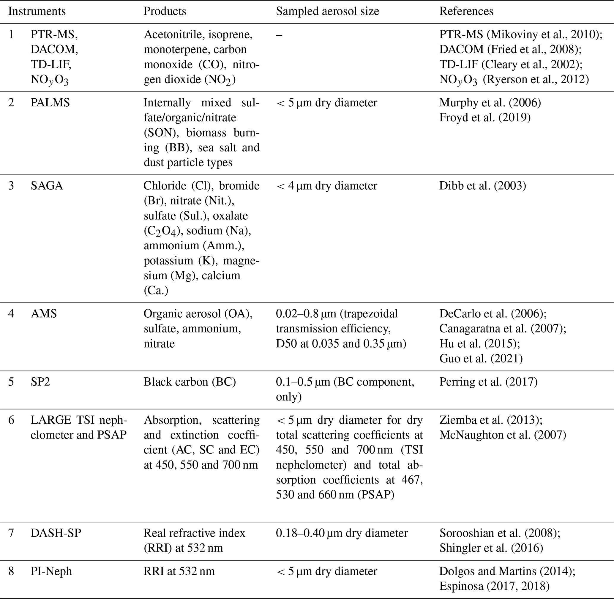
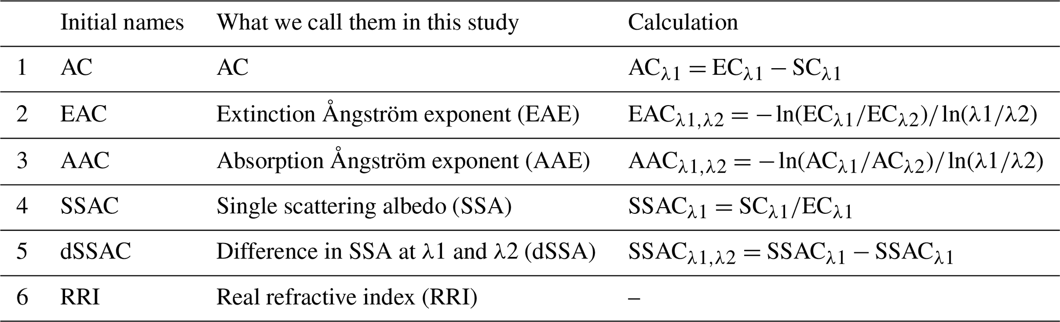
In this study, we use the 16 aerosol optical parameters listed in Table 2 (i.e., five first parameters at three wavelengths or three combinations of wavelengths and last parameter at 532 nm) and derived from the optical instruments in lines 6–8 of Table 1.
Table 2In situ optical parameters used in this study (provided at a given aircraft altitude by the instruments in lines 6–8 of Table 1), the way we call them in this paper, and how they are computed. The way we call these parameters is closer to what would be observed from remote sensing instruments. In the calculations, λ1 and λ2 are two given wavelengths. In this paper, we compute (i) SSA and AC at 450, 550 and 700 nm; (ii) EAE, AAE and dSSA between 450–550, 550–700 and 450–700 nm; and (iii) RRI at 532 nm.
Instead of simply using the standardized SEAC4RS merged dataset, a lot of effort was dedicated to carefully collocate, combine, cloud-screen, filter, and humidify datasets (i.e., convert from dry to ambient conditions), as well as compute and interpolate/extrapolate optical parameters to specific wavelengths (see Sect. A1.1 and A1.2).
2.2 Method
Figure 1 illustrates the overall method in this study, which involves following the five steps described below.
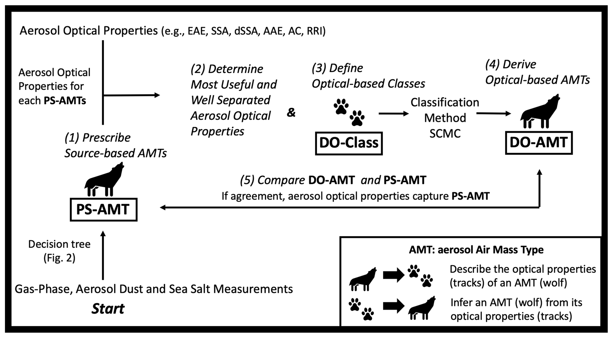
Figure 1Overall method in this study. PS-AMTs: prescribed source-based air mass types (AMTs); DO-Classes: defined optical-based class definitions; DO-AMTs: derived optical-based AMTs; EAE: extinction Ångström exponent; SSA: single scattering albedo; dSSA: difference in SSA; AAE: absorption Ångström exponent; AC: absorption coefficient; RRI: real refractive index; SCMC: pre-specified clustering and Mahalanobis classification. The concept of the wolf and its tracks is based on the dragon and its tracks in Bohren and Huffman (2008).
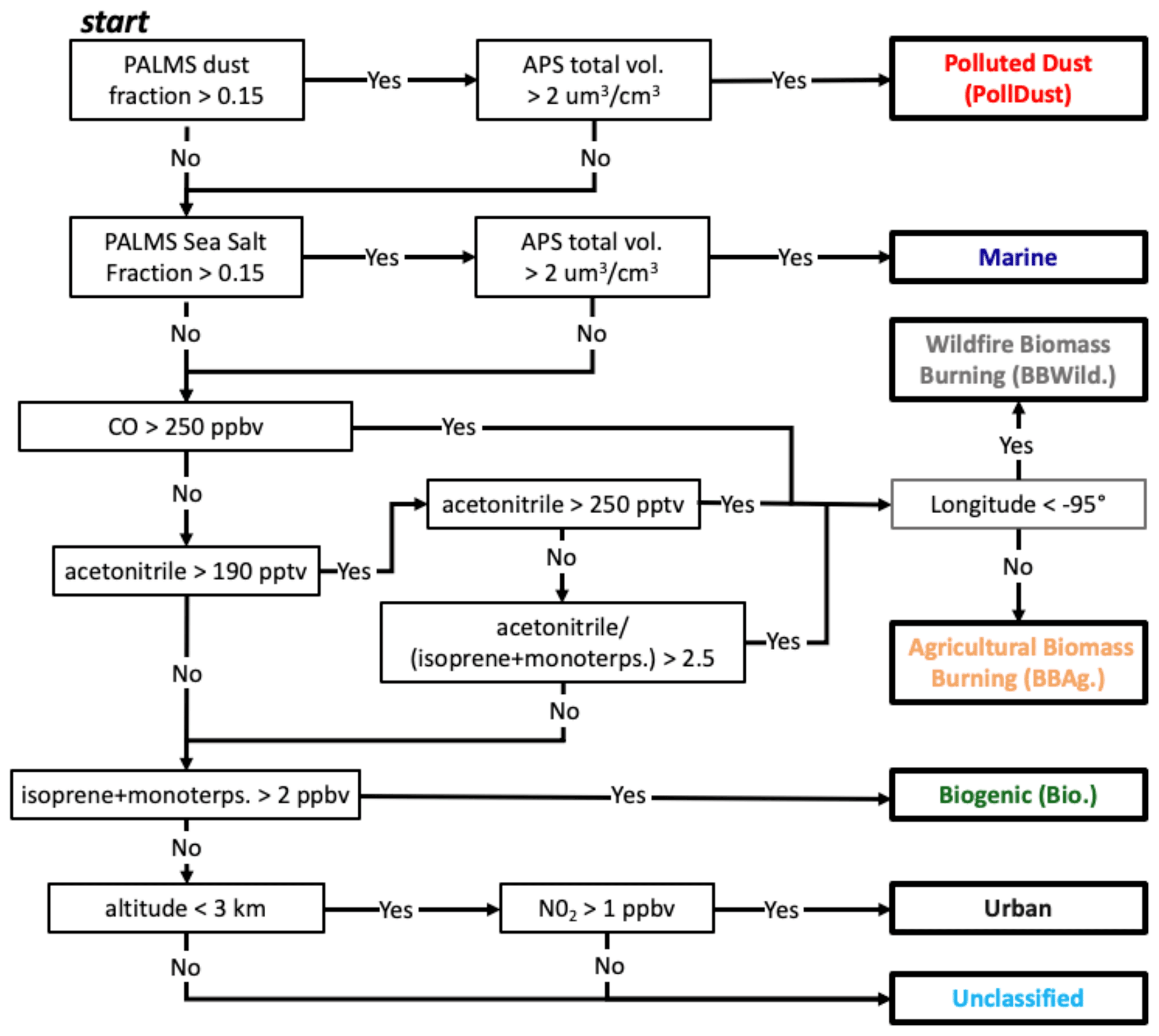
Figure 2Scheme to pre-specify air mass types (PS-AMTs; step 1 of Fig. 1) using mostly gas measurements and a method based on Espinosa et al. (2018) and Shingler et al. (2016) but modified to include marine and two different types of BB AMTs (i.e., BBAg. and BBWild.).
-
Prescribe source-based aerosol air mass types (called PS-AMTs). The PS-AMTs are defined using the gas-phase and aerosol instruments in lines 1–2 of Table 1 and a method based on Espinosa et al. (2018) and Shingler et al. (2016) illustrated in Fig. 2. These aerosol and gas measurements better characterize the aerosol properties in these AMTs compared to observations of aerosol optical properties. First, we define polluted dust PS-AMT (called PollDust) using PALMS dust number fraction (i.e., PALMS MineralFrac_PALMS) above 0.15 and the integrated dry aerosol volume concentration by the TSI aerodynamic particle sizer (APS) above 2 µm3 cm−3 (i.e., IntegV_Daero-PSL_APS_LARGE; note that APS measurements sampled dry aerodynamic diameters ranging from 0.56 to 6.31 µm; Espinosa et al., 2018). Similarly, we define marine PS-AMTs when PALMS sea salt number fraction >0.15 and total volume >2 µm3 cm−3. The remaining observations may then be evaluated for BB PS-AMTs using PTR-MS acetonitrile, WAS isoprene_WAS, PTR-MS isoprene-furan, PTR-MS monoterpenes, WAS CO_WAS and DACOM CO_DACOM if (i) acetonitrile ppbv or (ii) (acetonitrile ppbv) and (acetonitrile/(isoprene + monoterpene) >2.5) or (iii) CO >250 ppbv. BB PS-AMTs are further differentiated as coming from agricultural fires (called BBAg.) if the longitude is east of or from wildfires (called BBWild.) if the longitude is west of . The longitude threshold was selected according to the location of agricultural fires in Liu et al. (2016). If observations are not classified as PollDust or BB, we classify them as biogenic (called Bio.) if isoprene + monoterpene >2 ppbv. Finally, remaining observations are classified as urban if the altitude is below 3 km and NO2 >1 ppbv (i.e., using the NOAA nitrogen oxides and ozone (NOyO3), NO2_ESRL or TD-LIF NO2_TD-LIF). Section 3.1 describes these PS-AMTs, their location and composition during SEAC4RS.
-
Determine most useful and well-separated aerosol optical properties. Once the PS-AMTs are defined, we test whether these PS-AMTs exhibit distinct aerosol optical properties and then select the most useful and well-separated aerosol optical properties. This step and the following steps use the optical parameters listed in Table 2 and provided by the instruments listed in lines 6–8 of Table 1. To select the most useful and well-separated aerosol optical properties for each PS-AMT, we define a cluster in multi-dimensional parameter space, which is composed of all the data points (values of optical properties) in that PS-AMT category. Then, for each point in the dataset, we calculate the nearest cluster using the Mahalanobis distance (Mahalanobis, 1936). If the nearest cluster to a point corresponds to the PS-AMT, then that point is steady. This method was used in previous studies (e.g., Espinosa et al., 2018) and is described in further detail in Sect. A1.3. Section 3.2 describes the results from this step, i.e., the most useful and well-separated aerosol optical properties in our study.
-
Define optical-based training classes (called DO-Classes). We use the set of aerosol optical parameters defined in the second step above to define optical-based class definitions (called DO-Classes), including means, variances and covariances. In other terms, in this step, we form the mathematical definitions of the classes. The DO-Classes use the steady (i.e., well separated) points from the first half of all valid aerosol optical observations. Once the training clusters DO-Classes are defined, we use the Mahalanobis distance to filter outliers from our training dataset and further purify them. Similar to Russell et al. (2014), we delete points that have less than 1 % probability of belonging to each pre-specified DO-Class. We also delete from a specified cluster any points that are closer (in terms of Mahalanobis distance) to a different cluster. Note that unlike in Russel et al. (2014), this additional filtering step has a minimal impact on the training dataset in our study.
-
Derive optical-based aerosol air mass types (called DO-AMTs). The DO-AMTs are analyzed and classified using the set of aerosol optical properties defined in the second step above, the DO-Class defined in the third step and the SCMC method for a set of observations that was not included in the training datasets. This test dataset is based on independent observations and must be of the same nature as the training dataset. In this study, our test dataset is composed of independent airborne in situ optical properties. It is the other half of all valid aerosol optical observations (DO-Classes are defined using the steady portion of the first half). We derive DO-AMT for each test data point using the SCMC method and the DO-Class. This is achieved by assigning the test data point to the DO-Class that shows minimum Mahalanobis distance in a multi-dimensional space made of the best suited and most separable optical properties. Section 3.3 describes the results from this step.
-
Compare derived optical-based AMTs (DO-AMTs) and prescribed source-based AMTs (PS-AMTs). We evaluate the ability of airborne aerosol optical properties to successfully extract PS-AMTs by comparing PS-AMTs and DO-AMTs. Section 3.4 describes the results of this final step in our study.
In Fig. 1, we illustrate AMTs as wolves and their optical properties as their tracks. The second and third step consist in describing the optical properties (or tracks) of each AMT (or wolf). The fourth step consists in inferring an AMT (or wolf) from its optical properties (or tracks). The fifth and last step consist in comparing the inferred to the initial AMT (or wolf).
3.1 Prescribe source-based air mass types (PS-AMTs)
Figure 3 shows the PS-AMTs pre-specified using mostly measured gas-phase compounds and the method described in Fig. 2.
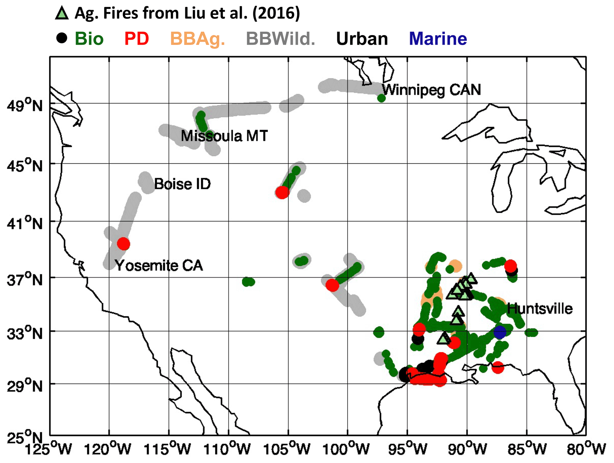
Figure 3Air mass types pre-specified (PS-AMT) using mostly gas measurements and methods based on Espinosa et al. (2018) and Shingler et al. (2016) (see Fig. 2). The number of data points assigned to each PS-AMTs are N=31 BBAg., N=382 BBWild., N=646 Bio. and N=46 PollDust PS-AMTs. PS-AMTs marine and urban were not analyzed in the remainder of this study due to their limited number of data points (N=9 urban in black and N=7 marine in blue). Green triangles show the location of agricultural fires according to Liu et al. (2016).
During SEAC4RS, according to Kim et al. (2015) and Wagner et al. (2015), the campaign-averaged aerosol mass was composed of mostly OA that is internally mixed with sulfate and nitrate at all altitudes over the SEUS i.e., 55 % OA and 25 % sulfate mass on average according to ground-based filter-based PM2.5 (particulate matter concentration with an aerodynamic diameter smaller than 2.5 mum) speciation measurements from the US EPA Chemical Speciation Network. This is consistent with the findings of Edgerton et al. (2006), Hu et al. (2015), Xu et al. (2015) and Weber et al. (2007) which show that PM2.5 is dominated by SOA and sulfate during the summer in SEUS. Aircraft data show that 60 % of the aerosol column mass (i.e., mostly OA and sulfate) is contained within the mixing layer (Kim et al., 2015).
GEOS-Chem attributes OA mass as 60 % from biogenic isoprene and monoterpenes sources (with a significant role of isoprene in accordance with Hu et al., 2015; Marais et al., 2016; Zhang et al., 2018; Jo et al., 2019; and Liao et al., 2015), 30 % from anthropogenic sources, and 10 % from open fires (Kim et al., 2015). Espinosa et al. (2018) confirm the domination of biogenic emissions in the SEUS (see their Fig. 2). Figure 3, in agreement with these studies, shows a majority of biogenic PS-AMTs (in green, N=646), mostly in the SEUS.
During SEAC4RS, the air sampled by the DC8 was also affected by both long-range transport of wildfire from the west (Peterson et al., 2015; Saide et al., 2015; Forrister et al., 2015; Liu et al., 2017) and local agricultural fires mostly from the burning of rice straw along the Mississippi River Valley (Liu et al., 2016). Figure 3, in agreement with these studies, shows BBWild. PS-AMT in the west (in grey, N=382) and BBAg. PS-AMT in the east (in salmon, N=31). Both agricultural and wildfire smoke are mainly composed of OA, which includes a substantial amount of light-absorbing brown carbon (Liu et al., 2017), produced mostly by smoldering combustion (Reid et al., 2005; Laskin et al., 2015).
Although Fig. 3 also shows urban and marine PS-AMTs in the SEUS, these PS-AMTs were not further analyzed in the remainder of this study due to their limited number of data points (urban in black with N=9 and marine in blue with N=7 data points).
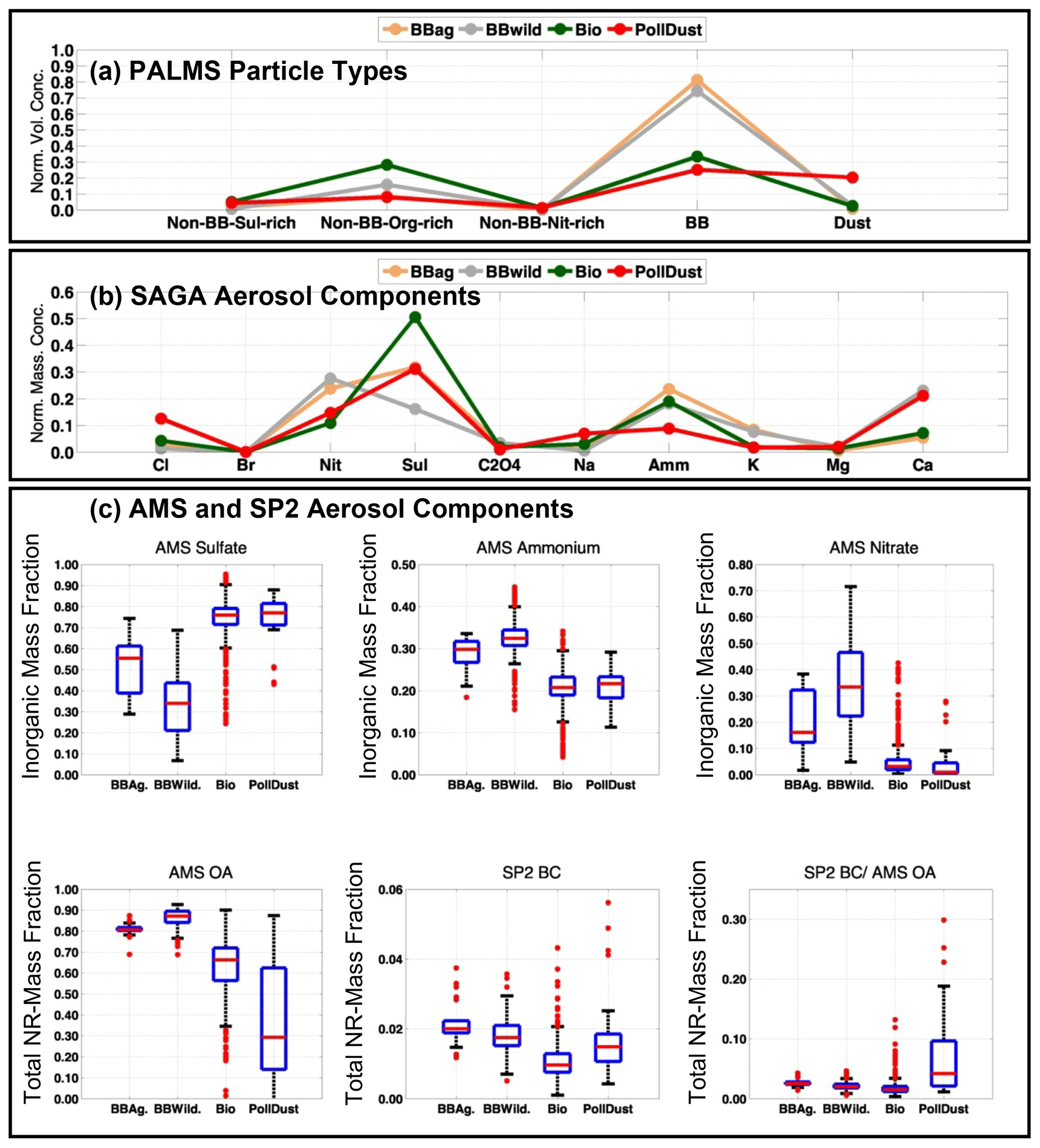
Figure 4(a) Average PALMS normalized volume concentration per PS-AMT. PALMS normalization uses the sum of BB particles, sulfate-, organic- and nitrate-rich particles from non-BB sources, mineral dust, sulfate–organic–nitrate (SON) particles without a dominant sub-component, and sea salt (the latter two PALMS aerosol types are not shown and constitute the remainder). (b) Averaged and normalized SAGA mass concentrations per PS-AMT; normalization uses the sum of all the SAGA components in the x axis; Cl: chloride; Br: bromide; Nit.: nitrate; Sul.: sulfate; C2O4: oxalate; Na: sodium; Amm.: ammonium; K: potassium; Mg: magnesium; Ca: calcium. (c) Normalized mass fractions of AMS sulfate, ammonium, nitrate, OA, SP2 BC, and ratio of SP2 BC and AMS OA per PS-AMT. The AMS inorganic mass fraction of sulfate, ammonium and nitrate is normalized to the sum of sulfate, ammonium and nitrate. The AMS and SP2 total non-refractory (NR) mass fraction of OA and BC is normalized to the sum of OA, BC, sulfate, ammonium and nitrate. In each blue box, the red horizontal line indicates the median, and the bottom and top edges of the box indicate the 25th and 75th percentiles, respectively. The black whiskers extend to the most extreme data points not considered outliers, and the outliers are plotted individually using red points. PS-AMTs marine and urban are not analyzed due to their limited number of data points (N=9 urban and N=7 marine PS-AMTs).
Figure 4 describes the aerosol chemical signatures of the principal PS-AMTs using the PALMS, SAGA, AMS and SP2 instruments (see lines 2–5 in Table 1 for more information on these instruments and their products). Note that some aerosol components (e.g., OA, sulfate, nitrate) are very general chemical indicators and much less specific than the gas-phase chemistry they are trying to predict. These aerosol components are nonetheless directly comparable to aerosol chemical components simulated in CTMs.
Note that the four aerosol instruments in Fig. 4 measure different aerosol properties. For instance, AMS and SAGA measure bulk concentrations of chemical sub-components (e.g., sulfate), whereas PALMS classifies individual particles into several size-resolved types, including mineral dust, BB and several non-BB types that have varying amounts of internally mixed sulfate, organic and nitrate.
The PS-AMTs in Fig. 4 show expected chemical features.
-
The BB PS-AMTs (i.e., BBAg. and BBWild.) record high BB particle concentrations from PALMS in Fig. 4a; high nitrate (Nit.), ammonium (Amm.), calcium (Ca.) and potassium (K) concentrations from SAGA in Fig. 4b; high OA (i.e., >0.8) from AMS; and high BC mass fractions from SP2 in Fig. 4c, in agreement with many other studies (e.g., Cubison et al., 2011; Hecobian et al., 2011; Jolleys et al., 2015; Guo et al., 2020). The BB PS-AMTs also record higher AMS ammonium and nitrate, compared to Bio. and PollDust PS-AMTs in Fig. 4c. This is due to ammonium nitrate forming in fires by neutralization of freshly formed nitric acid from NOx oxidation with an excess of primary ammonia (e.g., Guo et al., 2020).
-
The Bio. PS-AMTs record higher non-BB organic-rich particles from PALMS in Fig. 4a, higher SAGA sulfate concentrations in Fig. 4b, and smaller nitrate and ammonium (i.e., relatively acidic) and higher sulfate particle concentrations (from, e.g., coal plants) from AMS in Fig. 4c, compared to the BB PS-AMTs. As such, the Bio. PS-AMTs in this study are typical of the SEUS region (e.g., Kim et al., 2015, and Hu, 2015). When using positive matrix factorization (Ulbrich et al., 2009) on the AMS measurements, most of the organic aerosols in the Bio. PS-AMTs are composed of biogenic SOA. The Bio. PS-AMTs also record significantly lower BC concentrations from the SP2 as well as BC-to-OA ratios from the AMS and SP2 in Fig. 4c, compared to the BB and PollDust PS-AMTs, in accordance with, e.g., Hodzic et al. (2020).
-
The PollDust PS-AMTs record, as expected, high dust concentration from PALMS in Fig. 4a and high calcium (Ca) and magnesium (Mg) from SAGA in Fig. 4b. In addition, the PollDust PS-AMTs also include BB from PALMS in Fig. 4a and possibly a minor sea salt component (i.e., high sodium, Na, and chloride, Cl) from SAGA in Fig. 4b as well as relatively high sulfate from SAGA and AMS in Fig. 4c. A compositional picture of the PollDust PS-AMTs from PALMS in Sect. A2.3 shows dust predominately in the coarse mode but also an accumulation mode that contains a variety of particle types, all of which contain sulfate and organic material.
The analysis in Fig. 4 confirms that the gas-phase-derived PS-AMTs indeed have distinct aerosol chemical properties. Therefore, we explore whether these PS-AMTs can be derived using only aerosol optical properties.
3.2 Determine most useful and well-separated aerosol optical properties
As described in Sect. 2.2, we need to test if the PS-AMTs from Sect. 3.1 exhibit distinct aerosol optical properties. This is an essential step to optimize the final prediction of AMTs using aerosol optical properties (DO-AMTs).
We start with the 16 aerosol optical parameters in Table 2 (i.e., EAE, SSA, dSSA, AAE and AC at different combinations of 450, 550 and 700 nm and RRI at 532 nm). Section A2.1 illustrates the ranges of these 16 aerosol optical parameters, classified by PS-AMTs. Given that many of these parameters have similar properties, we select 6 out of these 16 aerosol optical parameters to simplify the analysis and presentation of results. To do that, we first look at the percentage of points unambiguously retrieved or steady (i.e., points that are well separated from other clusters and, hence, remain in their initial clusters) when using different combinations of 2 out of 16 aerosol optical parameters across all four PS-AMTs. We first select parameters AAE between 450 and 550 nm and RRI at 532 nm as they form the only combination of two parameters to achieve >65 % steady points for all four PS-AMTs (see Fig. A5). The rest of the six optical parameters are either chosen at 550 nm (i.e., closest wavelength to 532 nm) or between 450 and 550 nm. As a result, the six parameters we choose for the remainder of this study are dSSA 450–550 nm, RRI 532 nm, EAE 450–550 nm, AAE 450–550 nm, SSA 550 nm and AC at 550 nm. Among these parameters, the usefulness of parameters dSSA 450–550 nm, EAE 450–550 nm, SSA 550 nm and AC at 550 nm only becomes apparent in a 3-D parameter space (see Fig. A6 and its orange boxes, which record >65 % steady points for many combinations of three parameters among these six selected aerosol optical parameters).
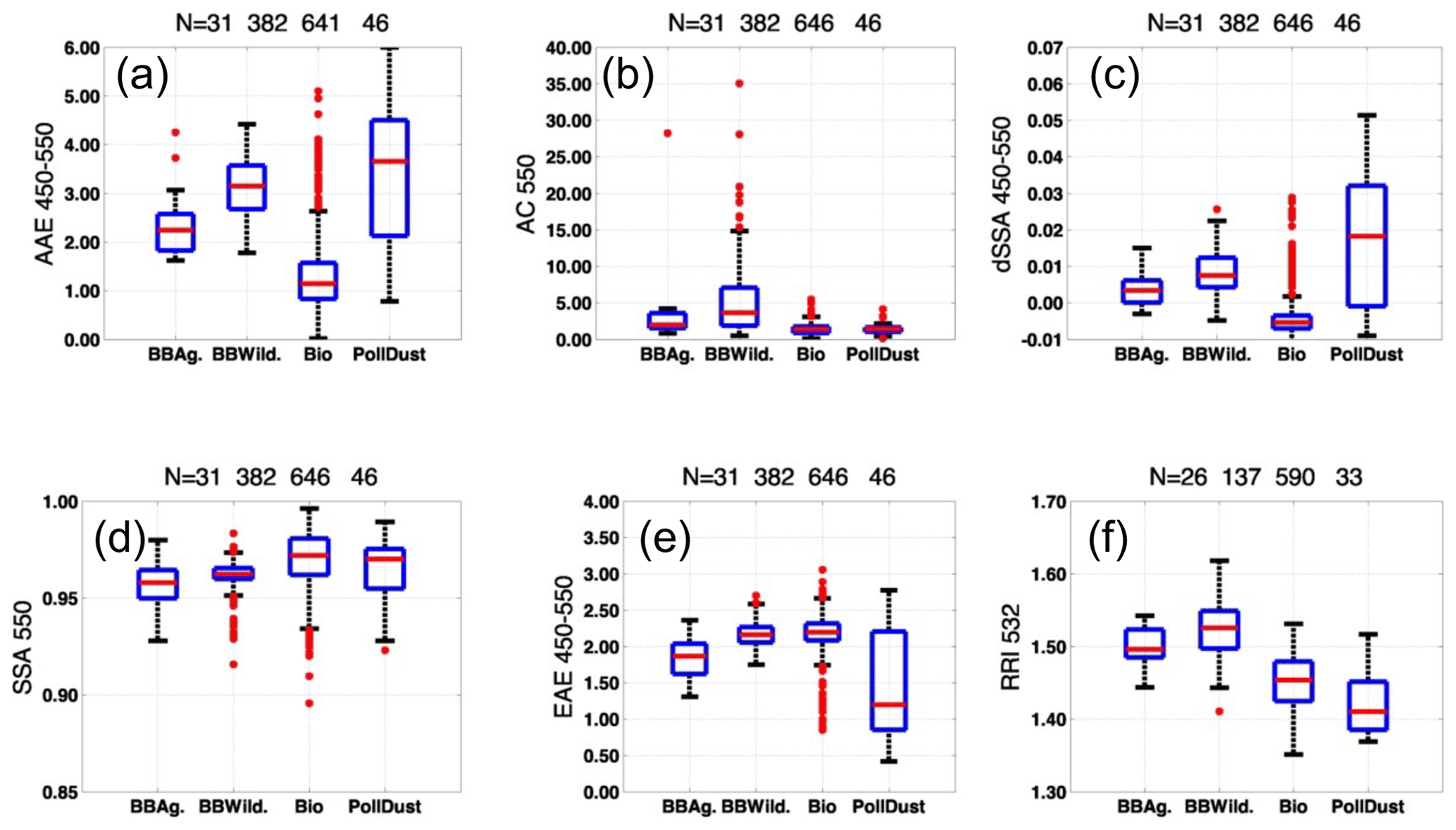
Figure 5Optical characterization of PS-AMTs using the LARGE, PI-Neph and DASH-SP instruments (see Table 1). In each blue box, the red horizontal line indicates the median, and the bottom and top edges of the box indicate the 25th and 75th percentiles, respectively. The black whiskers extend to the most extreme data points not considered outliers, and the outliers are plotted individually using red points. (a) AAE: absorption Ångström exponent; (b) AC: absorption coefficient; (c) dSSA: difference in single scattering albedo; (d) SSA: single scattering albedo; (e) EAE: extinction Ångström exponent; (f) RRI: real refractive index. Numbers in the title correspond to the number of points behind each box–whisker plot for the respective BBAg., BBWild., Bio. and PollDust PS-AMTs.
Figure 5 illustrates the range of these six aerosol optical properties for each PS-AMT. Fine particles (i.e., BBWild., BBAg. and Bio. PS-AMTs with higher EAE values) show mostly well-separated variability in RRI, AAE and dSSA. Coarse particles (i.e., PollDust PS-AMT with lower EAE values) are optically distinctive from the other PS-AMTs, particularly showing lower RRI, higher AAE and higher dSSA. In agreement with Selimovic et al. (2019, 2020) in Missoula, MT, we seem to also observe separate optical signatures and more specifically different AAE ranges for BBAg. and BBWild. PS-AMTs during SEAC4RS.
The aerosol optical properties of the PollDust PS-AMTs in this study differ from the ones of the pure dust AMT in Russel et al. (2014). The pure dust in Russel et al. (2014) is based on AERONET measurements in various dusty regions of the world. In this study, PollDust PS-AMTs show a median EAE of ∼1.3 between 450 and 550 nm and a median RRI of ∼1.4 at 532 nm in Fig. 5, compared to ∼0 between 491 and 864 nm and 1.53 at 670 nm for AERONET-based pure dust in Russel et al. (2014). We show that the higher PollDust PS-AMT EAE values in our study are due to the presence of accumulation-mode non-dust aerosols, which constitute a significant contribution to the total number and volume concentration of particles (see Fig. A7 for a compositional picture of PollDust PS-AMT). Similarly, we also suggest that the low PollDust PS-AMT RRI values are due to its non-dust accumulation mode, which is generally more hygroscopic than pure dust and may have a larger contribution to the PollDust total growth factor. We refer the reader to Fig. A4 for a closer look at RRI values in the case of PollDust PS-AMTs from the PI-Neph and DASH-SP instruments separately.
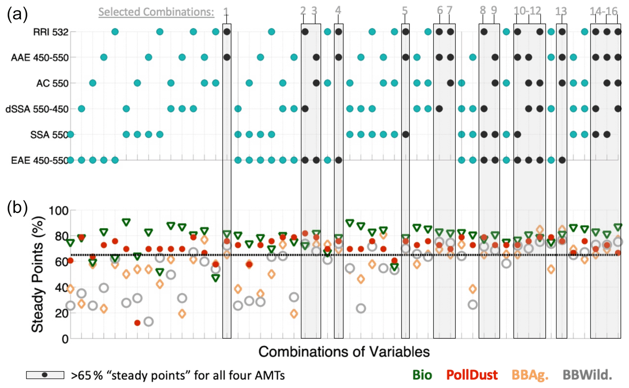
Figure 6Percentage of steady points (i.e., fraction of cases of a given type that are correctly identified) in panel (b) when using different combinations of aerosol optical parameters in panel (a) for each PS-AMT. Grey boxes and black points depict combinations of optical parameters showing >65 % steady points for PS-AMTs BBAg., BBWild., Bio. and PollDust. RRI: real refractive index; AAE: absorption Ångström exponent; AC: absorption coefficient; dSSA: difference in single scattering albedo; SSA: single scattering albedo; EAE: extinction Ångström exponent.
Figure 6 shows steady values (i.e., fraction of cases of a given type that are correctly identified) for combinations of two, three and four optical parameters out of the six selected aerosol optical parameters in Fig. 5 and four AMTs (i.e., BBAg., BBWild., Bio. and PollDust). Moving forward, we select the 16 combinations of optical parameters highlighted by grey boxes and black dots in Fig. 6, as they show >65 % steady points for PS-AMTs BBAg., BBWild., Bio. and PollDust. These combinations are numbered in grey at the top of Fig. 6.
Let us note that for some cases, the fraction of steady points seems to decrease when adding classifying variables. These cases were investigated and are mostly due to fewer data points that are non-steady when adding classifying parameters, out of an already small total number of data points (e.g., a combination of EAE, dSSA, AAE and RRI shows <65 % steady points for BBAg. PS-AMT, compared to >65 % steady points for a combination of EAE, AAE and RRI; this is due to four more steady points (N=18) when using a combination of three parameters, compared to four parameters (N=14), out of a total of N=26 cases).
Moreover, we suggest that higher aerosol loadings within the air masses allow for more accurate identification by optical properties, due to higher accuracy of the aerosol optical properties themselves. For example, we have seen an increase from ∼80 % to 100 % steady data points in the BBWild. PS-AMT when using EAE, AAE and RRI when extinction coefficients increased from 30–40 to 60–70 Mm−1 (number of data points between N=11 and N=20).
3.3 Define optical-based class definitions and derive optical-based air mass types (DO-Classes and DO-AMTs)
Next, we derive AMTs (DO-AMTs) followed by a comparison between DO-AMTs and the initial PS-AMTs to test the ability of aerosol optical properties alone to capture PS-AMTs.
As described in Sect. 2.2, to derive DO-AMTs using the SCMC method, we need (i) a combination of useful and well-separated optical properties (e.g., EAE, AAE and RRI or combination no. 4 in Fig. 6), (ii) a set of defined classes of reference (i.e., a training dataset that we call DO-Class) and (iii) the computation of the Mahalanobis distance between each observation we want to classify in a test dataset and each of the clusters from the training dataset.
We introduce Table 3, which records the number of data points behind each step in our study.
Table 3Number of data points per AMT behind each step in our study. PS-AMTs marine and urban are not analyzed due to their limited number of data points (N=9 urban and N=7 marine PS-AMTs). EAE: extinction Ångström exponent; AAE: aerosol absorption exponent; RRI: real refractive index.

* In the case of combination no. 4 in Fig. 6, i.e., EAE, AAE and RRI.
The first line of Table 3 shows the number of data points per PS-AMT (see Fig. 3). Then, lines 2, 3 and 4 of Table 3 show the valid number of AAE, RRI and a combination of EAE, AAE and RRI data points. Line 5 of Table 3 shows the steady number of data points per PS-AMT in the case of a combination of EAE, AAE and RRI (see Fig. 6). To create the training dataset DO-Class (line 7 in Table 3), we select the steady portion of half (every other sample) of the entire set of valid data points (line 6 in Table 3). The test dataset that we want to classify as DO-AMTs is the other half of the entire set of valid data points (line 8 in Table 3). This DO-AMT dataset is made of steady and non-steady data points.
Figure 7 illustrates the separability of the DO-Class in the 3-D space made of aerosol optical parameters EAE, AAE and RRI. The regions of the DO-Class are described by colored ellipses representing the mean, variance, and covariance of the DO-Class training set. It also shows that most of the DO-Classes represent the original source-based PS-AMTs (represented by colored triangles in Fig. 7). However, let us note that a distinct portion of the Bio. PS-AMTs (green triangles) seems to not be represented by the Bio. DO-Class (green ellipse). These Bio. PS-AMTs show higher AAE and lower EAE values and mostly fall into the PollDust DO-Class instead (red ellipse).
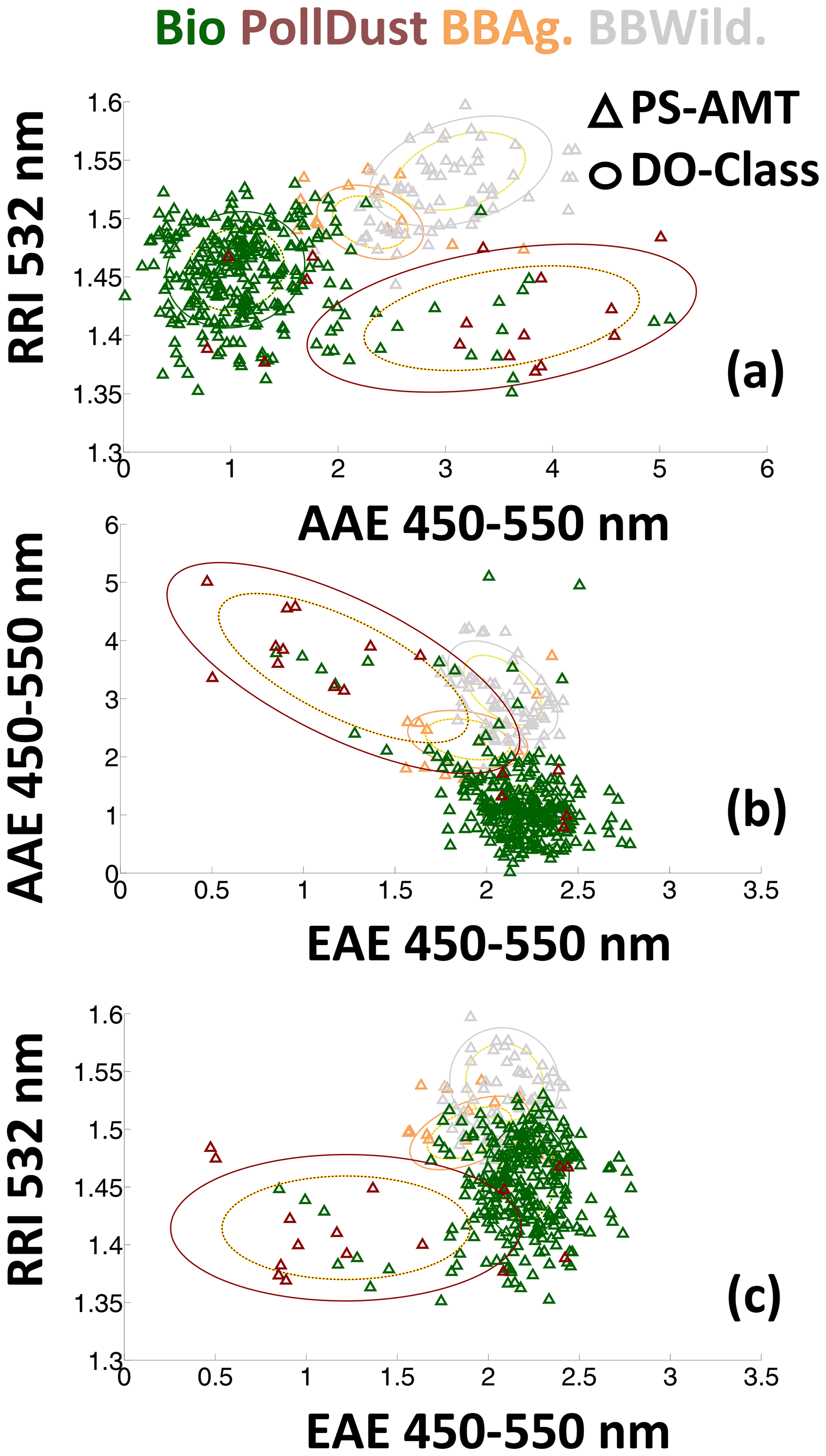
Figure 7DO-Class definition (solid and dashed ellipses colored by AMTs defining boundaries of the DO-Class clusters; DO-Class data points are not plotted) and prescribed source-based PS-AMTs (triangles colored by AMTs). A total of 75 % of the DO-Classes are contained in the solid ellipses, and 50 % of the DO-Classes are contained in the dashed ellipses. RRI: real refractive index; AAE: absorption Ångström exponent; EAE: extinction Ångström exponent. Panels (a)–(c) illustrate PS-AMT and DO-Class in the respective 2-D spaces made of AAE-RRI, EAE-AAE and EAE-RRI.
Line 9 in Table 3 shows the number of DO-AMTs (correctly and incorrectly) classified as BBAg., BBWild., Bio. or PollDust AMTs using the combination of EAE, AAE and RRI as an example, the SCMC method, and the DO-Class reference clusters. Most points from the test dataset were assigned an AMT (see N=381 assigned DO-AMTs on line 9, compared to N=8 unknown on line 10 of Table 3). Unclassified/unknown DO-AMTs are those where the 3-D data point is outside the 99 % probability surface for all four DO-Classes.
3.4 Compare optical-based and source-based air mass types (DO- vs. PS-AMTs)
Once we have derived DO-AMTs from optical properties (i.e., inferred our wolf based on its tracks in Fig. 1), we need to assess how many of the DO-AMTs agree with those originally assigned as PS-AMTs. Line 11 in Table 3 shows the number of prescribed PS-AMTs in each category when only looking at the test dataset to derive DO-AMTs on line 8 of Table 3 (N=389). Line 12 in Table 3 shows the number of DO-AMTs that are identical to PS-AMTs. Lines 13 and 14 show the same result but as a percentage of the respectively derived DO-AMTs or prescribed PS-AMTs in the same category. In Table 3, we find 77 % BBAg., 79 % BBWild., 73 % Bio. and 81 % PollDust PS-AMTs are correctly reflected in the DO-AMTs. This result can also be seen for combination no. 4 in Fig. 8 (i.e., EAE, AAE and RRI).
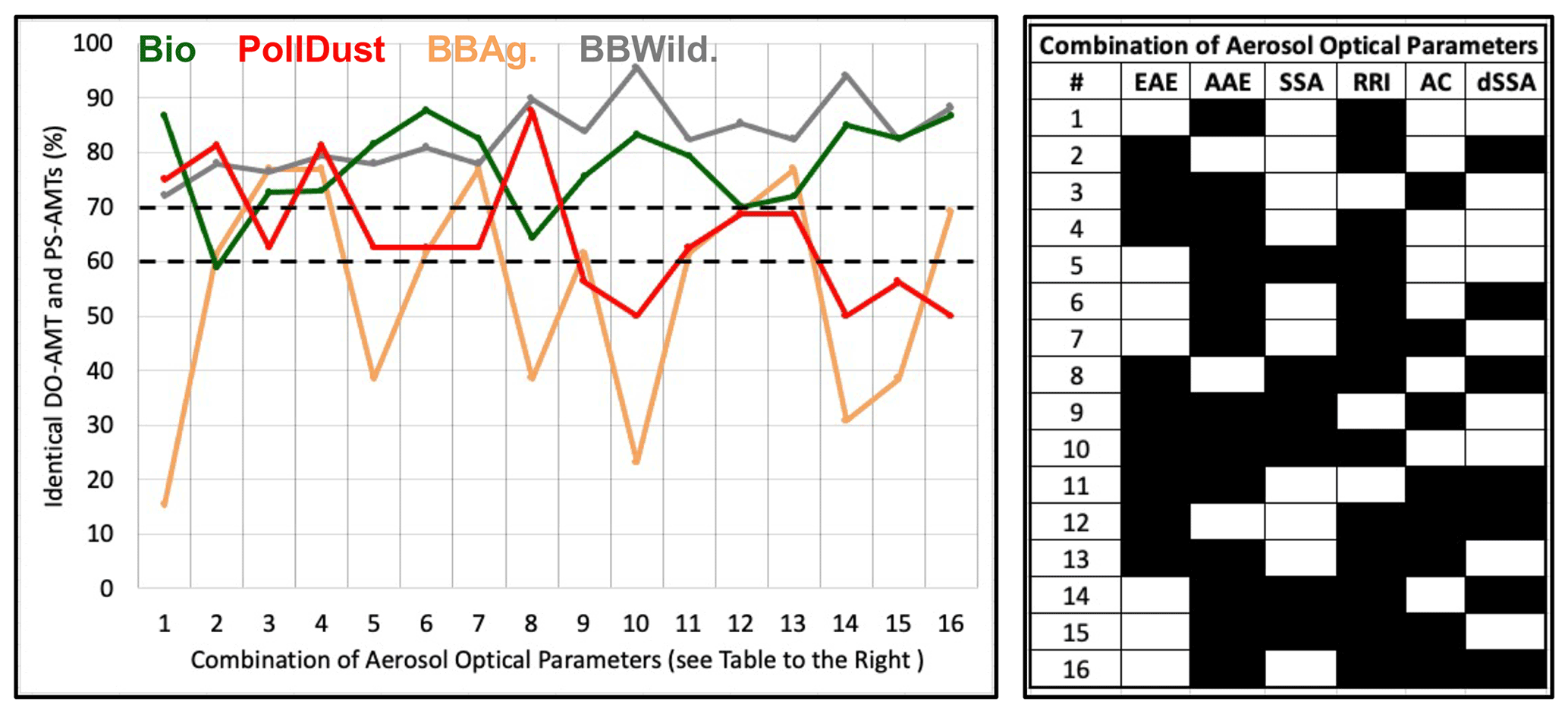
Figure 8Identical DO-AMTs and PS-AMTs as a percentage of prescribed PS-AMTs in each category when using the different combinations of optical parameters listed in the table to the right (black squares show combination on each line) and for the four PS-AMTs BBAg. (salmon), BBWild. (grey), Bio. (green) and PollDust (red). Black horizontal dashed lines show 60 % and 70 % identical DO-AMT and PS-AMTs.
Figure 8 illustrates the percentage of identical DO-AMTs to PS-AMTs when using each of the 16 combinations of optical parameters illustrated by black squares in the table of Fig. 8. These combinations are the same as the ones in grey at the top of Fig. 6. This percentage, like line 14 in Table 3, is computed as the number of DO-AMTs that agree with those originally assigned as PS-AMTs, compared to the total number of prescribed PS-AMTs in each category in our test dataset (e.g., line 11 in Table 3).
According to Fig. 8, the entire 16 combinations of aerosol optical properties listed in the Table of Fig. 8 as black squares seem to capture both the Bio. and BBWild. PS-AMTs ( % identical DO-AMT and PS-AMTs in green and grey solid lines in Fig. 8). We remind the reader that these PS-AMTs are mostly based on gas measurements (see Fig. 2) and are dominated by different aerosol species (see Fig. 4).
On the other hand, fewer combinations of aerosol optical parameters seem to adequately capture the BBAg. and PollDust PS-AMTs. Further analysis shows that, on average, most DO-AMTs assigned to the BBAg. and PollDust categories are, in fact, misclassified and fail to capture the Bio. PS-AMTs. As shown earlier in Fig. 7, we suggest these DO-AMTs fail to capture the Bio. PS-AMTs because the Bio. DO-Class might not be entirely representative of the Bio. PS-AMTs (see green triangles outside of the green ellipses in Fig. 7).
Note that three combinations of aerosol optical parameters, namely no. 4 (EAE, AAE and RRI), no. 12 (EAE, RRI, AC and dSSA) and no. 13 (EAE, AAE, RRI and AC) in Fig. 8, seem to capture all four PS-AMTs particularly well ( % identical DO-AMTs and PS-AMTs). Let us mention that results linked to the use of the absorption coefficient, AC, an extensive property that is dependent on aerosol loading, is likely to be unique to this study and might not be representative of any other field campaign.
We suggest that a similar study should be performed using data from additional airborne field campaigns which have the necessary, or equivalent, gas-phase measurements to derive source-based AMTs and many of the critical optical properties to extract optical-based AMTs. First, this would provide more robust statistics – e.g., particular attention should be given to revisit the BB from agricultural fires and polluted dust AMTs in this study. Second, this would provide more AMTs/sub-AMTs to analyze – e.g., urban and marine AMTs should be visited during CAMP2EX (Clouds, Aerosol and Monsoon Processes Philippines Experiment) or KORUS-AQ (An International Cooperative Air Quality Field Study in Korea), and other types of BB and at different aging stages should be visited during FIREX-AQ (Fire Influence on Regional to Global Environments and Air Quality). Finally, this would also help assess if these chemical and optical signatures are reproducible from one year to another.
In this study, we obtained in situ aerosol optical signatures. Another essential step should be to examine optical signatures from a space-based passive remote sensor(s), which derive total column effective ambient aerosol optical properties (instead of properties measured at the altitude of the aircraft in this study). One way to answer this question would be to compare the defined optical-based classes (DO-Classes) signatures using collocated airborne in situ aerosol optical properties and total column aerosol optical properties measured or inferred by sun photometry (e.g., airborne 4STAR, Spectrometers for Sky-Scanning Sun-Tracking Atmospheric Research, Dunagan et al., 2013; or ground-based AERONET). This DO-Class database could then be used as an optical-based training dataset to enable widespread derivation of optical-based AMTs (DO-AMTs) using existing and future orbital and suborbital remote sensing instruments and networks.
The space mission addressing the designated observable Aerosols, Cloud, Convection and Precipitation (ACCP) from the NASA decadal survey (National Academies of Sciences, Engineering, and Medicine, 2019) is currently designing its suborbital (airborne and ground-based) component to address science questions that cannot be addressed from space (e.g., bridging satellite-inferred aerosol optical properties and aerosol speciation). This study illustrates how essential it is to explore existing airborne datasets to bridge chemical and optical signatures of different AMTs before the implementation of future spaceborne missions and their corresponding suborbital field campaign(s) – e.g., upcoming spaceborne polarimeters SPEXone (Hasekamp et al., 2019) and Hyper-Angular Rainbow Polarimeter (HARP-2) on board the NASA Plankton, Aerosol, Cloud, ocean Ecosystem (PACE) (Werdell et al., 2019) and the multi-viewing multi-channel multi-polarization imager (3MI) (Fougnie et al., 2018) to be launched in the next 3 years or the next generation of Earth Observing System (EOS) satellites addressing NASA's ACCP.
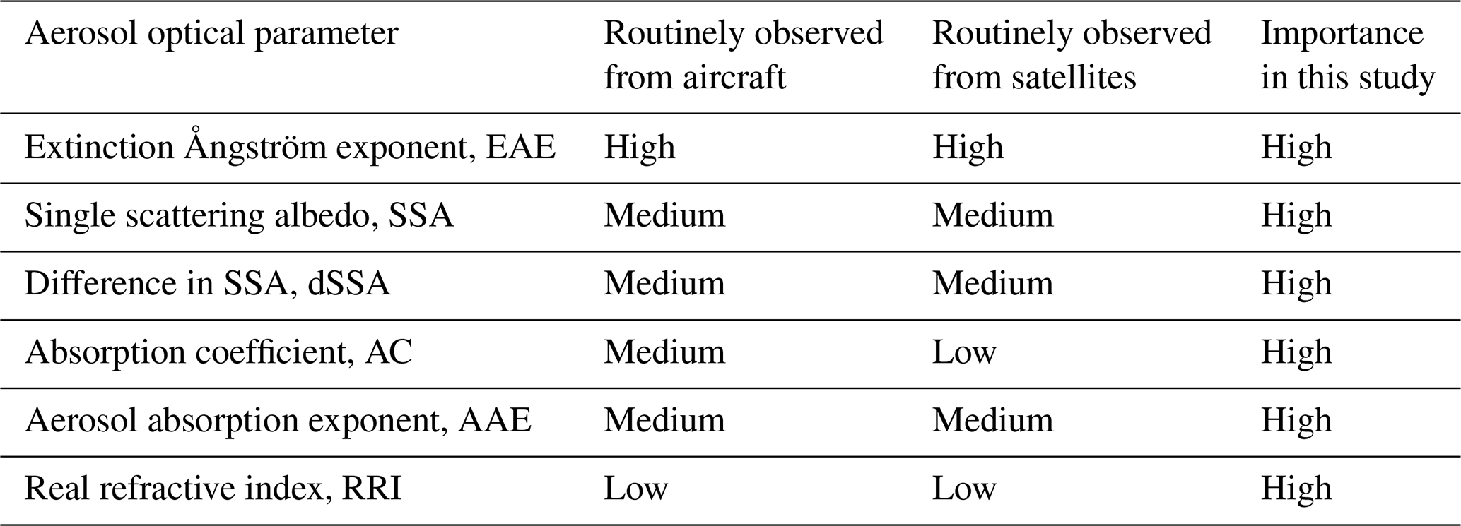
Most of the six optical properties in this study (i.e., extinction Ångström exponent, single scattering albedo, difference of single scattering albedo, absorption coefficient, absorption Ångström exponent and real part of the refractive index) are routinely derived by in situ and remote sensing instrumentation/networks (see Table 4). Some optical properties are more likely to present a higher uncertainty when measured from suborbital field campaigns and/ or from satellites. The real part of the refractive index, for example, although generally more uncertain, is highly desirable in many combinations of optical parameters to capture both the BB from wildfires and biogenic AMTs in this study. We strongly suggest future airborne campaigns consider including in situ measurements of AAE and RRI (very few of the campaigns to date flew PI-Neph and/or DASH-SP instruments), and a special attention should be given to deriving these parameters accurately from space. Our analysis has the advantage of providing alternate combinations of optical parameters when one optical parameter is either not available or too uncertain.
Table 4Frequency at which the six aerosol optical parameters in our study are routinely derived from aircraft and current passive satellite sensors and importance of these optical parameters in our study. RRI: real refractive index; AAE: absorption Ångström exponent; AC: absorption coefficient; dSSA: difference in single scattering albedo; SSA: single scattering albedo; EAE: extinction Ångström exponent.
Ultimately, this technique and its results has the potential to provide a much broader observational aerosol dataset to evaluate global transport models than is currently available. Current satellite-derived AMTs seem to marginally help models. One way to assess models would be to directly compare satellite-derived AMTs to AMTs derived from modeled optical properties (which are, in turn, computed from modeled chemical composition) using the same classification method (e.g., Taylor et al., 2015; Dawson et al., 2017; Nowottnick et al., 2015; Meskhidze et al., 2021). However, it would be difficult to define the main source of errors in the case of a disagreement between model- and observation-based AMTs. Potential causes of such a disagreement could be a combination of observation and method-specific errors or model-specific errors (e.g., the assumed model size distribution, dry refractive index, growth factor per species, mass extinction efficiency per species, estimated mass per species, RH, transport, chemical processing, emissions and other physiochemical variables). Let us emphasize that the technique and results in this study, alone, will not be able to fully explain any discrepancies between model and observations. However, we suggest that the use of near-simultaneous gas-phase, chemical and optical instruments on the same aircraft restrict the causes of a disagreement between model- and observation-based AMTs to mostly model-specific errors. Moreover, as the AMTs in this study are less ambiguously defined (e.g., to each AMT corresponds an averaged distribution of aerosol chemical composition), we suggest that this may allow the assessment (and, by extension, improvement) of a few aerosol processes simulated in CTMs.
One desire of our scientific community is to ultimately translate the space-based total atmospheric column effective AMTs such as biomass burning, dust, urban industrial, and polluted marine into chemical species with defined emission source inventories and formation/aging chemistry such as sulfate, BC, OA, SOA, nitrate, dust, or sea salt to better improve models. Fully achieving that goal might not be feasible, and progress can only be incremental. This study constitutes a first step towards the goal of translating the space-based total atmospheric column effective aerosol optical properties and derived optical-based AMTs into source-based AMTs.
Current satellite-derived AMTs inferred by various techniques are useful to provide spatial context to support other observations of aerosols and clouds or evaluate other aerosol type classifications. However, these satellite-derived AMTs are ambiguously defined and might often be misclassified.
The AMTs in this study are defined, characterized and derived using gas-phase, chemical and optical instruments on the same aircraft. This reduces errors in measurements/retrievals due to spatiotemporal colocation and ambiguities in the selection of the AMT training dataset. We also specifically investigate the strengths and weaknesses of various aerosol optical properties used as tools to define AMTs and how much these optical properties can capture dominant aerosol speciation.
We first define AMTs using mostly airborne gas-phase measurements during SEAC4RS. We find distinct optical signatures for biomass burning (from agricultural/prescribed or wildfires), biogenic and dust-influence AMTs (marine and urban AMTs show too few data points to analyze). Useful aerosol optical properties to characterize these signatures are the extinction Ångström exponent between 450–550 nm, the single scattering albedo at 550 nm, the difference of single scattering albedo in two wavelengths between 450–550 nm, the absorption coefficient at 550 nm, the absorption Ångström exponent between 450–550 nm and the real part of the refractive index at 532 nm. We then use these aerosol optical properties, prescribe a well-separated AMT training dataset, and use the pre-specified clustering and Mahalanobis classification method to derive optical-based AMTs during SEAC4RS. We find that by using any of 16 combinations of these six optical parameters, over 65 % of two AMTs (i.e., optical-based wildfire biomass burning and biogenic) agree with their source-based analog. We find that four AMTs (i.e., biogenic, BB from wildfires, BB from agricultural fires, and polluted dust), when prescribed using mostly airborne in situ gas measurements, can be successfully extracted from at least three combinations of airborne in situ aerosol optical properties over the US during SEAC4RS, such that more than 70 % of optical observations are typed consistently with source-based analog. However, we find that misclassifications are not evenly distributed across the classes, and specifically the optically based classifications for BB from agricultural fires and polluted dust include a large percentage of misclassifications that limit the usefulness of results relating to those classes.
A1 Additional information on methods
A1.1 Method to cloud-screen, filter and humidify airborne observations
This section describes the cloud-screening, filtering, humidification and colocation involved in the computation of the final set of 16 optical parameters (i.e., EAE, dSSA and AAE between 450–550, 550–700 and 450–700 nm; AC and SSA at 450, 550 and 700 nm; and the RRI at 532 nm) in this study.
The LARGE TSI nephelometer and PSAP instruments operate under dry conditions. The only measurement provided at ambient conditions is the EC at 532 nm. In this work, we need LARGE EC and SC at 450, 550 and 700 nm at ambient conditions. To do that, we use the parameter fRH550_RH20to80 at 550 nm provided by the LARGE f(RH) system (different from the TSI or PSAP instruments) and an exponential curve to obtain the impact of hygroscopic growth on the aerosol light scattering coefficient, i.e., the scattering enhancement factor f(RH) at 450, 550 and 700 nm. Ambient SC at 550 nm, for example, is computed as the product of dry SC at 550 nm and f(RH) at 550 nm. We filter out any values of LARGE dry SC at 450 nm≤10 Mm−1 and LARGE ambient SSAC at 863 nm≤0.7.
DASH-SP provides measurements of RRIDASH−SP_dry, information on the particle hygroscopicity, κDASH−SP_dry, and the particle diameter, DpDASH−SP_dry, in dry conditions. We compute DASH-SP RRI in ambient conditions, RRIDASH−SP_ambient, using RRIDASH−SP_dry, κDASH−SP_dry, and the ambient relative humidity and temperature measurements, RHHSKP and THSKP, provided by the AIMMS-20 (Aircraft-Integrated Meteorological Measurement System) or 3D-winds instruments. First, we vary the growth factor, GFvar, from 1.02 to 1.5 by increments of 0.01 and compute the particle hygroscopicity, κvar, for given RHHSKP, THSKP and DpDASH−SP_dry measurements as follows:
where
-
%GF
-
-
;
-
kg mol−1
-
R=8.3144598
-
ρw=1000 kg m−3.
We select the growth factor, GFvar, that provides the closest κvar value to the κDASH−SP_dry measurement. We call this growth factor GFselect. Finally, we compute the ambient RRI, RRIDASH−SP_ambient, using RRIDASH−SP_dry and GFselect obtained in the previous steps and Eq. (5) of Mallet et al. (2003) (based on Hänel, 1976) as follows:
where RRIw=1.33. Let us note that Aldhaif et al. (2018) demonstrate the limitations of using the volume-weighted mixing rule approach above, especially in the presence of OA.
The PI-Neph provides measurements of dry phase function (P11) and the second element of the scattering phase matrix (P12) at three wavelengths over an angular range spanning . These measurements are fed into the GRASP (Dubovik et al., 2014) algorithm to obtain retrieved values of spectral complex refractive index, a parameterized size distribution and derived optical properties like scattering coefficients. In this work we utilize these optical properties provided by PI-Neph in dry conditions: the SC at 532 nm, SCPI−Neph_dry; the dry size distribution, dNdlnrPI−Neph_dry; and the refractive index, RIPI−Neph_dry. First, we compute the target ambient SC at 532 nm, SCPI−Neph_target, as the product of SCPI−Neph_dry and LARGE f(RH) measurements at 550 nm. Second, we compute the ambient SC at 532 nm, SCPI−Neph_ambient, corresponding to each GFvar from 1 to 1.5 by increments of 0.01 using (i) a Mie code (Mishchenko et al., 2002) and, as input to the Mie code, (ii) the ambient size distribution and corresponding radii, computed from dNdlnrPI−Neph_dry and GFvar, (iii) the ambient refractive index computed from RIPI−Neph_dry and GFvar (see Eq. A2) and a prescribed geometric standard deviation (i.e., ∼1.12, which results in similar computed and provided SCPI−Neph_dry values when using the same Mie code and initial parameters dNdlnrPI−Neph_dry and RIPI−Neph_dry). Third, we select GFvar (we call this growth factor GFselect) and corresponding RRIPI−Neph_ambient that record the minimum difference between SCPI−Neph_ambient and SCPI−Neph_target.
We compute ambient AMS and SP2 mass concentrations using the parameter stdPT-to-AMB_Conversion_AMS-60s reported with the AMS data. SP2 BC standard concentration (referred to as refractory black carbon, and experimentally equivalent to elemental carbon at the 15 % level; Petzold et al., 2013; Kondo et al., 2011; Perring et al., 2017), originally in ng m−3, is converted into µg m−3 and scaled upwards, on a flight-by-flight basis, to represent the entire accumulation mode (on average by 1.14). The AMS sulfate, ammonium and nitrate are normalized to the sum of sulfate, ammonium and nitrate. The AMS OA and SP2 BC are normalized to the sum of OA, BC, sulfate, ammonium and nitrate. In the case of SAGA, bromide and chloride are set to zero if under the detection limit of 0.0107 and 0.0391 µg m3. In the case of PALMS, we use volume-weighted products (Froyd et al., 2019). In this study, PALMS particle classes include mineral dust, sea salt, biomass burning and sulfate–organic–nitrate mixtures (SON). The SON class was further refined into organic-rich, sulfate-rich and nitrate-rich particle types, plus a remainder of SON particles that did not exhibit a dominant chemical sub-component. To define the marine and polluted dust AMTs, PALMS composition was combined with aerosol size distribution data from LARGE to yield integrated volume fractions of mineral dust and sea salt particle types from µm based on the method of Froyd et al. (2019). The average AMT chemical composition is determined as a raw number fraction of particles observed by PALMS.
A1.2 Method to collocate airborne observations
All the airborne observations are cloud-screened using wing-mounted cloud probes. Table A1 defines three datasets used in this study with their associated number of data points, called AIRBO1, AIRBO2 and AIRBO3, and their combination, AIRBO. In all four datasets, the LARGE data are first collocated to housekeeping (HSKP) data (i.e., select same start_utc in seconds) and humidified/ filtered (see Sect. A1.1).
Table A1Definition of three datasets (AIRBO1, AIRBO2, AIRBO3) and their combination, AIRBO (which is the dataset used in this study); the airborne instruments involved during SEAC4RS (see Table 1); the co-located parameters (see Table 2 for a definition of EAE, SSA, dSSA, AC, AAE and RRI); and the number of data points showing valid aerosol optical properties and PS-AMT BBAg., BBWild., Bio. or PollDust.

In the AIRBO1 dataset, we compute the mean HSKP and LARGE values in a ±30 s range centered on each collocated AMS–PALMS–SP2 start_time (i.e., the 1 min merged file). We then record LARGE averaged values if (i) the average is made of at least 20 points and (ii) the standard deviation of the LARGE EAE is below 30 %. In the AIRBO2 dataset, we compute the mean HSKP and LARGE values between each DASH-SP start_utc and end_utc. We record HSKP, humidified LARGE and DASH-SP values if the following four parameters are below 30 %: (i) the standard deviation of the LARGE EAE, (ii) the difference between κDASH−SP_dry and κvar (Eq. A1), (iii) the standard deviation of RHHSKP, and (iv) the standard deviation of THSKP. In the AIRBO3 dataset, we compute the mean HSKP and LARGE values between each PI-Neph start_utc and end_utc. We record HSKP, humidified LARGE and PI-Neph values if the following four parameters are below 30 %: (i) the standard deviation of the LARGE EAE, (ii) the standard deviation on scatPI−Neph_dry, (iii) the standard deviation on LARGE f(RH), and the difference between PI-Neph SCPI−Neph_target and SCPI−Neph_ambient (see Sect. A1.1). Finally, we collocate the HSKP–LARGE–DASH-SP (HSKP–LARGE–PI-Neph) to the AMS–PALMS–SP2 datasets in the case of AIRBO2 (AIRBO3). To do that, if there are multiple AMS–PALMS–SP2 data points between each HSKP–LARGE–DASH-SP (HSKP–LARGE–PI-Neph) averaged time stamp, we average all AMS–PALMS–SP2 data between the HSKP–LARGE–DASH-SP (HSKP–LARGE–PI-Neph) averaged time stamps. If there are no multiple AMS–PALMS–SP2 data points between the HSKP–LARGE–DASH-SP (HSKP–LARGE–PI-Neph) averaged time stamps, we select the closest AMS–PALMS–SP2 data in time to the HSKP–LARGE–DASH-SP (HSKP–LARGE–PI-Neph) averaged time stamps. The dataset in this study, AIRBO, was obtained by first selecting common 1 min UTC time stamps from all three datasets and then arbitrarily selecting, in order of priority when present, AIRBO2, AIRBO1 and AIRBO3.
A1.3 Method to select most useful and well-separated aerosol optical properties
This section explains the second step of Fig. 1 in more details. Figure A1 is a simplified example to illustrate our method. It shows only two optical parameters (i.e., SSA and EAE) and three hypothetical PS-AMTs (e.g., pure dust in red, marine in blue and BB in green) measured by one hypothetical optical instrument in two different environments (defined by different locations and times, Fig. A1a–b vs. A1c–d). Figure A1a–b shows a smaller hypothetical range of EAE and SSA for the BB PS-AMT (green cluster), compared to Fig. A1c–d.
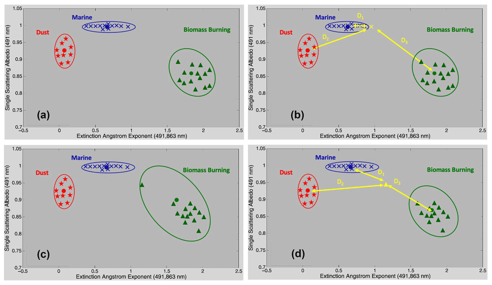
Figure A1Conceptual/hypothetical illustration of how we quantify separation between different air mass types and select the most useful and well-separated aerosol optical parameters. It shows three hypothetical PS-AMTs (e.g., dust in red, marine in blue and BB in green) measured by one hypothetical optical instrument in one environment (a–b) and in another environment (c–d). The EAE and SSA values in this illustration are based on AERONET observations (Russell et al., 2014) and are representative of typical pure dust, marine, and BB total column remote-sensing-inferred ground-based EAE and SSA values. Note that it only shows two dimensions even though some calculations of Mahalanobis distances (e.g., D1, D2, D3) will be made using more dimensions in this study.
To answer the question of how well these PS-AMTs (i.e., red, blue and green clusters in either Fig. A1a or c) are separated, we (i) select each data point separately (e.g., yellow crosses in Fig. A1b and d), (ii) recompute each PS-AMT cluster with the data point excluded (i.e., different blue PS-AMT in Fig. A1b and green PS-AMT in Fig. A1d compared to Fig. A1a and c) and calculate the Mahalanobis distance (Mahalanobis, 1936; Burton et al., 2012). The Mahalanobis distance is the distance between the data point in question (i.e., yellow crosses in Fig. A1b or d) and the position of each cluster center (i.e., red, blue and green clusters in Fig. A1b or d), which depends on cluster center, tilt and width in a multi-parameter space. These distances are called D1, D2 and D3 on either Fig. A1b or d. In the case of the yellow cross in Fig. A1b, distance D1 is the smallest, and the test point is reassigned to its original cluster. The test point is by consequence well separated from other clusters and steady. On the other hand, distance D1 is also the smallest in Fig. A1d, which means the test point (yellow cross) in Fig. A1d is not reassigned to its original cluster. The test point is by consequence not well separated from other clusters in this case and not steady. The steady fraction is the fraction of cases within each PS-AMT that are correctly identified. Steady fractions are used to assess separation between PS-AMTs. When including additional components (e.g., any other aerosol optical parameter from Table 2 in addition to SSA and EAE in Fig. A1), the additional number of steady points shows the component's relative importance in separating the PS-AMTs. The yellow points that are steady in Fig. A1 (i.e., correctly classified or well separated) are used to define the most useful and well-separated aerosol optical properties for each PS-AMT.
A2 Additional information on results
A2.1 Aerosol optical parameters classified by PS-AMT
This section describes the ranges of the 16 aerosol optical parameters (i.e., EAE, SSA, dSSA, AAE and AC at different combinations of 450, 550 and 700 nm and RRI at 532 nm from Table 2), classified by PS-AMTs in our study.

Figure A2EAE (450–700 nm, 450–550 nm, 550–700 nm) and AC (450, 550 and 700 nm) per PS-AMT. In each blue box, the red horizontal line indicates the median, and the bottom and top edges of the box indicate the 25th and 75th percentiles, respectively. The black whiskers extend to the most extreme data points not considered outliers, and the outliers are plotted individually using red points. Let us note that the LARGE EC measurements at 700 nm experienced issues during the latter half of SEAC4RS (Yohei Shinozuka, personal communication, 2018). AC: absorption coefficient; EAE: extinction Ångström exponent. Numbers in the title correspond to the number of points behind each box–whisker plot for the respective BBAg., BBWild., Bio. and PollDust PS-AMTs.
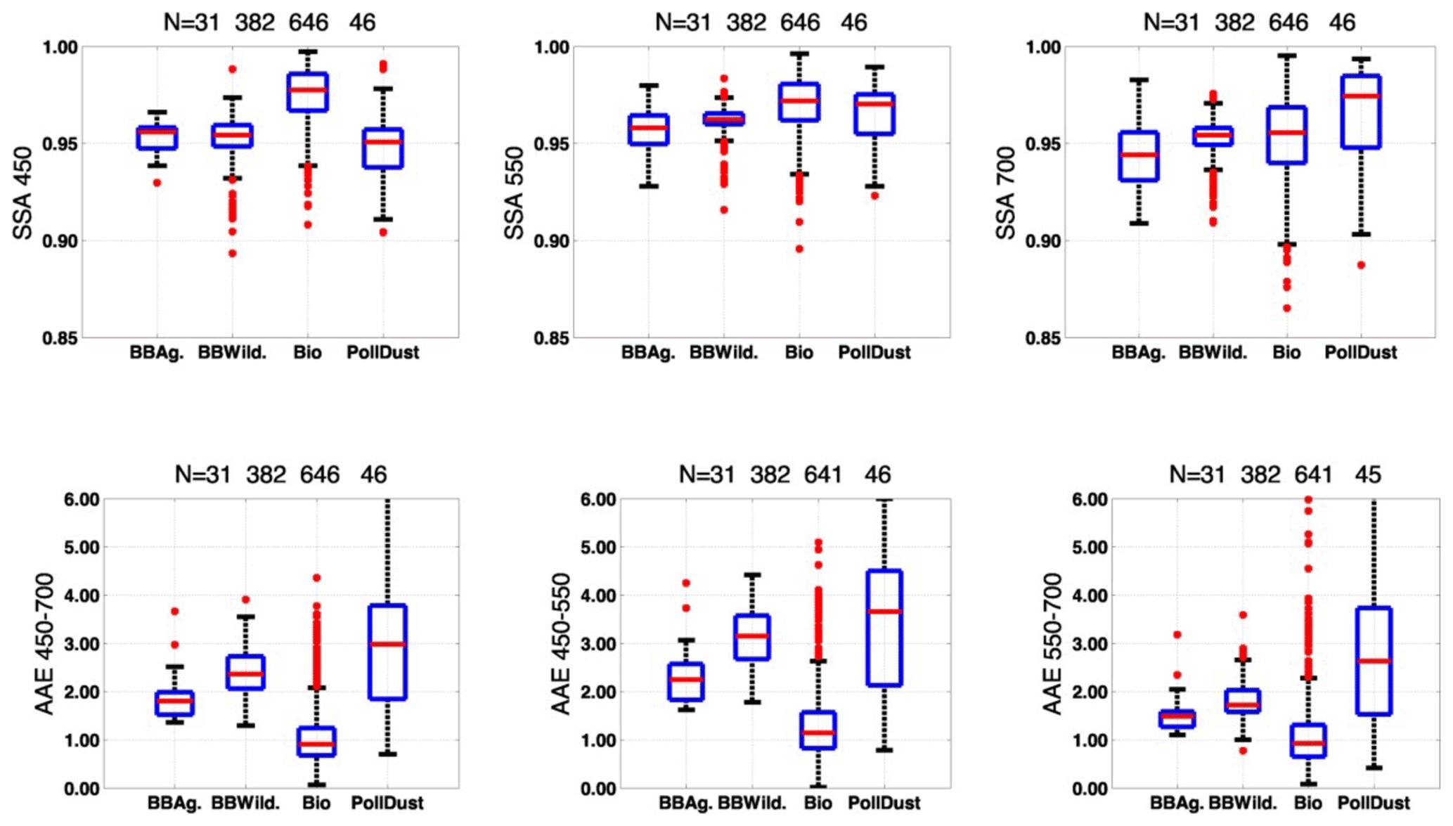
Figure A3SSA (450, 550 and 700 nm) and AAE (450–700 nm, 450–550 nm, 550–700 nm) per PS-AMT. In each blue box, the red horizontal line indicates the median, and the bottom and top edges of the box indicate the 25th and 75th percentiles, respectively. The black whiskers extend to the most extreme data points not considered outliers, and the outliers are plotted individually using red points. AAE: absorption Ångström exponent; SSA: single scattering albedo. Numbers in the title correspond to the number of points behind each box–whisker plot for the respective BBAg., BBWild., Bio. and PollDust PS-AMTs.

Figure A4The dSSA (700–450 nm, 550–450 nm, 700–550 nm), RRI (from DASH-SP and PI-Neph), RRI from DASH-SP and RRI from PI-Neph at 532 nm per PS-AMT. In each blue box, the red horizontal line indicates the median, and the bottom and top edges of the box indicate the 25th and 75th percentiles, respectively. The black whiskers extend to the most extreme data points not considered outliers, and the outliers are plotted individually using red points. RRI: real refractive index; dSSA: difference in single scattering albedo. Numbers in the title correspond to the number of points behind each box–whisker plot for the respective BBAg., BBWild., Bio. and PollDust PS-AMTs.
Note the slightly lower RRI values for DASH-SP compared to PI-Neph (i.e., respectively 1.41 and 1.43 at 532 nm in Fig. A4) in the case of PollDust PS-AMTs. We explain this difference in RRI values by different PollDust PS-AMT growth factor (GF) values. We obtain GF through two methods: (1) through the values directly measured by DASH-SP for particles in the size range 0.18< Dpdry<0.40 µm and (2) through an iterative procedure matching the output of a Mie code with dry PI-Neph retrievals and f(RH) measurements made by the LARGE group in parallel (see Sect. A1.1 for more details). We find a respective median PollDust PS-AMT GF value of ∼1.3 and ∼1.2 in the case of DASH-SP and PI-Neph, which we suggest is due to a smaller sampling size range for DASH-SP, compared to PI-Neph (see Table 1).
A2.2 Most useful and well-separated aerosol optical properties – 16 parameters
This section describes the percentage of points unambiguously retrieved or steady (i.e., points that are well separated from other clusters and, hence, reassigned to their initial clusters) when using different combinations of respectively 2 and 3 out of 16 aerosol optical parameters across all four principal PS-AMTs (i.e., provides more details to Sect. 3.2).
A2.3 Composition of our polluted dust (PollDust) PS-AMT
Figure A7 shows a compositional picture of the PollDust PS-AMTs from PALMS. The accumulation mode is a mixture of particle types, all of which contain sulfate and organic material. Coarse-mode dust particles account for most of the aerosol volume, whereas a non-dust accumulation mode contributes most to the total number concentration of particles.
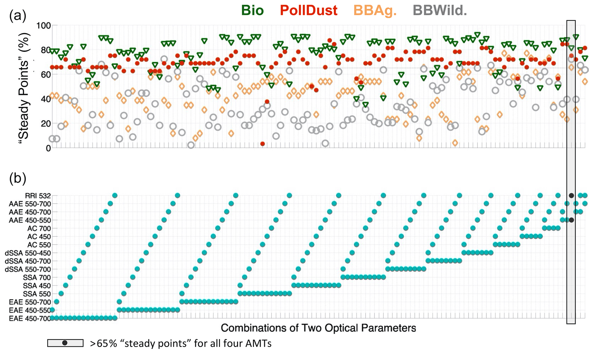
Figure A5Percentage of steady points (i.e., fraction of cases of a given type that are correctly identified; see Sects. 2.2 and A1.3 for more info) in panel (a) when using different combinations of two aerosol optical parameters in panel (b) for each PS-AMT. The grey box and black points are a combination of optical parameters showing >65 % steady points for PS-AMTs BBAg., BBWild., Bio. and PollDust. RRI: real refractive index; AAE: absorption Ångström exponent; AC: absorption coefficient; dSSA: difference in single scattering albedo; SSA: single scattering albedo; EAE: extinction Ångström exponent.
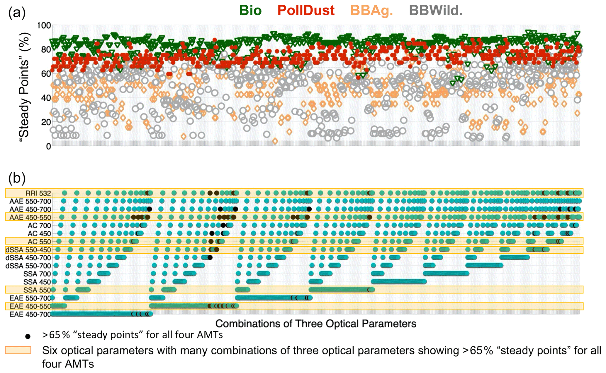
Figure A6Percentage of steady points (i.e., fraction of cases of a given type that are correctly identified; see Sects. 2.2 and A1.3 for more info) in panel (a) when using different combinations of three aerosol optical parameters in panel (b) for each PS-AMT. Black points are combinations of optical parameters showing >65 % steady points for PS-AMTs BBAg., BBWild., Bio. and PollDust. RRI: real refractive index; AAE: absorption Ångström exponent; AC: absorption coefficient; dSSA: difference in single scattering albedo; SSA: single scattering albedo; EAE: extinction Ångström exponent. Horizontal orange boxes show the six aerosol optical parameters that we have selected in this study.
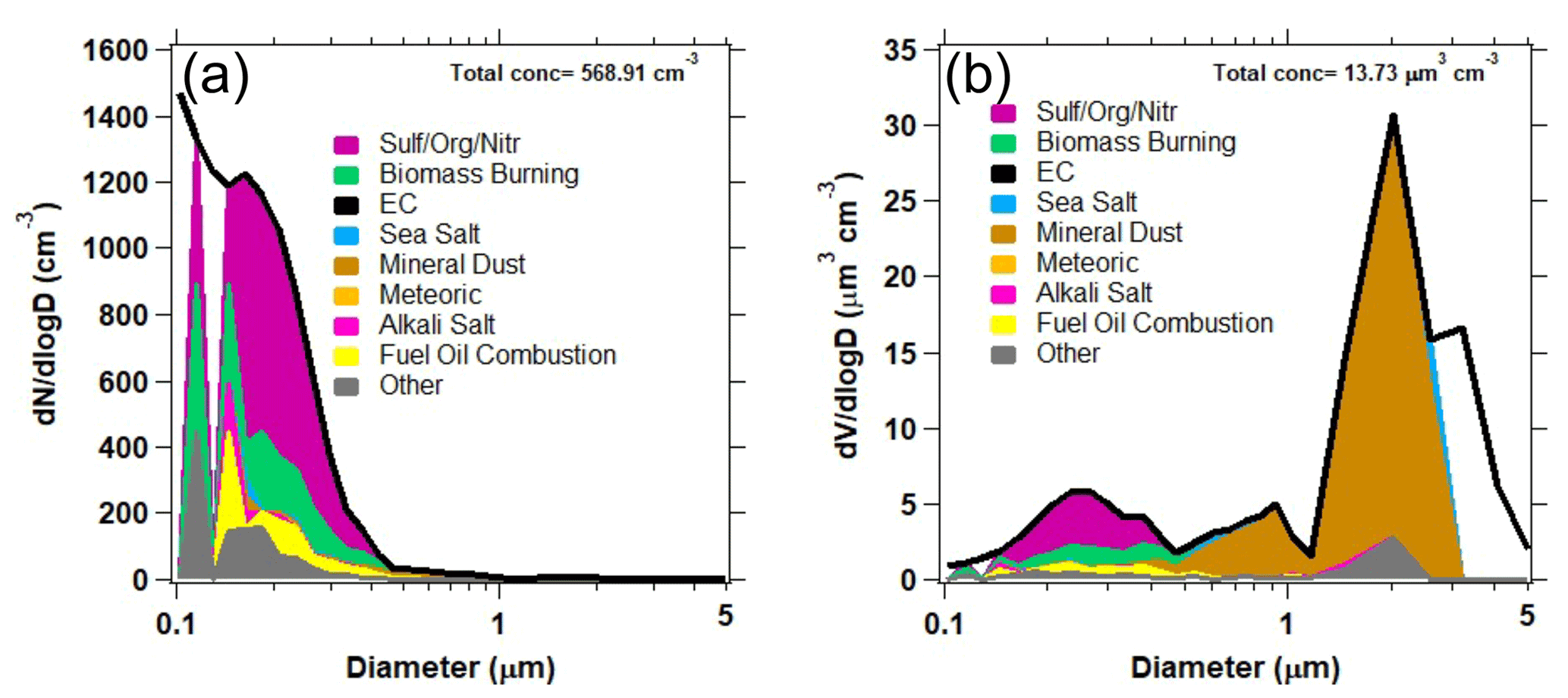
Figure A7PALMS particle classes are mapped to the total number (a) and volume (b) size distribution from LARGE based on the method of Froyd et al. (2019). Data include flight segments representative of the polluted dust PS-AMT.
| 3MI | Multi-viewing Multi-channel Multi-polarization imager |
| 4STAR | Spectrometers for Sky-Scanning Sun-Tracking Atmospheric Research |
| AAC | Absorption Ångström coefficient |
| AAE | Absorption Ångström exponent |
| AAOD | Aerosol absorption optical depth |
| AC | Absorption coefficient |
| ACCP | Aerosols, Cloud, Convection and Precipitation |
| AERONET | AErosol RObotic NETwork |
| AIMMS-20 | Aircraft-Integrated Meteorological Measurement System |
| Amm. | Ammonium |
| AMS | Aerosol mass spectroscopy |
| AMT | Air mass aerosol types |
| AOD | Aerosol optical depth |
| APS | TSI aerodynamic particle sizer |
| BB | Biomass burning air mass aerosol types |
| BBAg. | Biomass burning agricultural air mass aerosol types |
| BBWild. | Biomass burning wildfire air mass aerosol types |
| BC | Black carbon |
| Bio. | Biogenic air mass aerosol types |
| Br. | Bromide |
| C2O4 | Oxalate |
| Ca. | Calcium |
| CALIOP | Cloud-Aerosol Lidar with Orthogonal Polarization |
| CALIPSO | Cloud-Aerosol Lidar and Infrared Pathfinder Satellite Observation |
| CAMP2EX | Clouds, Aerosol and Monsoon Processes Philippines Experiment |
| Cl | Chloride |
| CO | Carbon monoxide |
| CTM | Chemical transport models |
| DACOM | Differential absorption carbon monoxide monitor |
| DASH-SP | Differential aerosol sizing and hygroscopicity spectrometer probe |
| DO-Classes | Defined optical-based classes |
| DO-AMTs | Optical-based air mass aerosol types |
| Dp | Particle diameter |
| dNdlnr | Particle size distribution |
| dSSA | Difference in SSA at two wavelengths |
| dSSAC | Difference in SSAC at two wavelengths |
| EAC | Extinction Ångström coefficient |
| EAE | Extinction Ångström exponent |
| EC | Extinction coefficient |
| EOS | Earth Observing System |
| FIREX-AQ | Fire Influence on Regional to Global Environments and Air Quality |
| GEOS-Chem | Goddard Earth Observing System model of atmospheric chemistry |
| GF | Growth factor |
| GRASP | Generalized Retrieval of Atmosphere and Surface Properties |
| HARP2 | Hyper-Angular Rainbow Polarimeter |
| HSKP | Housekeeping dataset |
| K | Potassium |
| κ | Particle hygroscopicity |
| KORUS-AQ | An International Cooperative Air Quality Field Study in Korea |
| LARGE | NASA Langley Aerosol Research Group Experiment TSI nephelometer and particle soot absorption photometer (PSAP) instruments |
| Mg | Magnesium |
| MODIS | Moderate Resolution Imaging Spectroradiometer |
| Na | Sodium |
| Nit. | Nitrate |
| NO2 | Nitrogen dioxide |
| NOyO3 | NOAA nitrogen oxides and ozone |
| OA | Organic aerosol |
| PACE | NASA Plankton, Aerosol, Cloud, ocean Ecosystem |
| PALMS | Particle analysis by laser mass spectrometry |
| PI-Neph | Polarized Imaging Nephelometer |
| PM2.5 | Particulate matter concentration with an aerodynamic diameter smaller than 2.5 µm |
| POLDER | Polarization and Directionality of Earth's Reflectances |
| PollDust | Polluted dust air mass aerosol types |
| PS-AMTs | Prescribed source-based air mass aerosol types |
| PTR-MS | High-temperature proton-transfer-reaction mass spectrometer |
| RFari | Radiative forcing due to aerosol–radiation interactions |
| RH | Relative humidity |
| RI | Complex refractive index |
| RRI | Real part of the refractive index |
| SAGA | Soluble Acidic Gases and Aerosol |
| SC | Scattering coefficient |
| SCMC | Pre-specified clustering and Mahalanobis classification method |
| SEAC4RS | Study of Emissions and Atmospheric Composition, Clouds, and Climate Coupling by Regional Surveys |
| SEUS | Southeastern US |
| SOA | Secondary organic aerosol |
| SON | Sulfate–organic–nitrate |
| SP2 | NOAA single particle soot photometer |
| SPEXone | Spectropolarimeter for Planetary Exploration orbital |
| SSA | Single scattering albedo |
| SSAC | Single scattering albedo coefficient |
| Sul. | Sulfate |
| T | Temperature |
| TD-LIF | Thermal dissociation and laser-induced fluorescence |
| US EPA | United Stated (of America) Environmental Protection Agency |
The SEAC4RS data used in this study are publicly available at the following link: https://doi.org/10.5067/Aircraft/SEAC4RS/Aerosol-TraceGas-Cloud (Chen, 2013).
The overarching research goals were formulated by MSFK. SPB, OPH, KDF, PCJ, MSJ, JR and GLS influenced the evolution of these research goals. Specific co-authors provided specific datasets and valuable help to interpret them (OPH for POLDER/PARASOL; KDF for PALMS; AJB, LZ, KLT and YS for LARGE; JED for SAGA; TS and AS for DASH-SP; RWE and VM for PI-Neph; JLJ and PCJ for AMS; and JPS for SP2). MSFK and QT carried out the formal analyses. MSFK carried out the investigations and visualizations and wrote the original draft. All co-authors have reviewed and edited the multiple drafts of the paper. The methodology behind the SCMC method was first developed by SPB and adapted to in situ data by MSFK.
At least one of the (co-)authors is a member of the editorial board of Atmospheric Chemistry and Physics. The peer-review process was guided by an independent editor, and the authors also have no other competing interests to declare.
Publisher’s note: Copernicus Publications remains neutral with regard to jurisdictional claims in published maps and institutional affiliations.
This research was supported by the NASA Atmospheric Composition Modeling and Analysis Program (ACMAP). We thank Richard Eckman for his support. We appreciate the efforts of all the SEAC4RS in situ instrument principal investigators involved in this study for obtaining, processing, documenting and disseminating their respective datasets. We also appreciate the comments of the reviewers that helped us to improve this article.
This research has been supported by the NASA Earth Sciences Division (grant nos. NNH14ZDA001N-ACMAP, 80NSSC21K1451 and 80NSSC19K0124).
This paper was edited by Yafang Cheng and reviewed by two anonymous referees.
Adhikary, B., Kulkarni, S., Dallura, A., Tang, Y., Chai, T., Leung, L. R. , Qian, Y., Chung, C. E., Ramanathan, V., and Carmichael, G. R.: A regional scale chemical transport modeling of Asian aerosols with data assimilation of AOD observations using optimal interpolation technique, Atmos. Environ., 42, 8600–8615, 2008.
Aldhaif, A. M., Stahl, C., Braun, R. A., Moghaddam, M. A., Shingler, T., Crosbie, E., Sawamura, P., Dadashazar, H., Ziemba, L., Jimenez, J. L., Campuzano-Jost, P., and Sorooshian, A.: Characterization of the Real Part of Dry Aerosol Refractive Index Over North America From the Surface to 12 km, J. Geophys. Res.-Atmos., 123, 8283–8300, https://doi.org/10.1029/2018JD028504, 2018.
Benedetti, A., Morcrette, J. J., Boucher, O., Dethof, A., Engelen, R. J., Fisher, M., Flentje, H., Huneeus, N., Jones, L., Kaiser, J. W., and Kinne, S.: Aerosol analysis and forecast in the European Centre for Medium-Range Weather Forecasts Integrated Forecast System: 2. Data assimilation, J. Geophys. Res.-Atmos., 114, D13205, https://doi.org/10.1029/2008JD011115, 2009.
Bohren, C. and Huffman, D.: Absorption and Scattering of Light by Small Particles John Wiley & Sons, New York, 544 pp., ISBN: 9783527618163, 2008.
Bond, T. C., Doherty, S. J., Fahey, D. W., Forster, P. M., Berntsen, T., DeAngelo, B. J., Flanner, M. G., Ghan, S., Kärcher, B., Koch, D., and Kinne, S.: Bounding the role of black carbon in the climate system: A scientific assessment, J. Geophys. Res.-Atmos., 118, 5380–5552, https://doi.org/10.1002/jgrd.50171, 2013.
Boucher, O., Randall, D., Artaxo, P., Bretherton, C., Feingold, G., Forster, P., Kerminen, V.-M., Kondo, Y., Liao, H., Lohmann, U., Rasch, P., Satheesh, S. K., Sherwood, S., Stevens, B., and Zhang, X. Y.: Clouds and aerosols, in: Climate Change 2013: The Physical Science Basis. Contribution of Working Group I to the Fifth Assessment Report of the Intergovernmental Panel on Climate Change, edited by: Stocker, T. F., Qin, D., Plattner, G.-K., Tignor, M., Allen, S. K., Doschung, J., Nauels, A., Xia, Y., Bex, V., and Midgley, P. M.: Cambridge University Press, United Kingdom and New York USA, 571–657, https://doi.org/10.1017/CBO9781107415324.016, 2013.
Buchard, V., Randles, C. A., Da Silva, A. M., Darmenov, A., Colarco, P. R., Govindaraju, R., Ferrare, R., Hair, J., Beyersdorf, A. J., Ziemba, L. D., and Yu, H.:The MERRA-2 aerosol reanalysis, 1980 onward. Part II: Evaluation and case studies, J. Climate, 30, 6851–6872, 2017.
Burton, S. P., Ferrare, R. A., Hostetler, C. A., Hair, J. W., Rogers, R. R., Obland, M. D., Butler, C. F., Cook, A. L., Harper, D. B., and Froyd, K. D.: Aerosol classification using airborne High Spectral Resolution Lidar measurements – methodology and examples, Atmos. Meas. Tech., 5, 73–98, https://doi.org/10.5194/amt-5-73-2012, 2012.
Canagaratna, M. R., Jayne, J. T., Jimenez, J. L., Allan, J. D., Alfarra, M. R., Zhang, Q., Onasch, T. B., Drewnick, F., Coe, H., Middlebrook, A., Delia, A., Williams, L. R., Trimborn, A. M., Northway, M. J., DeCarlo, P. F., Kolb, C. E., Davidovits, P., and Worsnop, D. R.: Chemical and microphysical characterization of ambient aerosols with the aerodyne aerosol mass spectrometer, Mass Spectrom. Rev., 26, 185–222, https://doi.org/10.1002/mas.20115, 2007.
Chen, C., Dubovik, O., Henze, D. K., Lapyonak, T., Chin, M., Ducos, F., Litvinov, P., Huang, X., and Li, L.: Retrieval of desert dust and carbonaceous aerosol emissions over Africa from POLDER/PARASOL products generated by the GRASP algorithm, Atmos. Chem. Phys., 18, 12551–12580, https://doi.org/10.5194/acp-18-12551-2018, 2018.
Chen, C., Dubovik, O., Henze, D. K., Chin, M., Lapyonok, T., Schuster, G. L., Ducos, F., Fuertes, D., Litvinov, P., Li, L., Lopatin, A., Hu, Q., and Torres, B.: Constraining global aerosol emissions using POLDER/PARASOL satellite remote sensing observations, Atmos. Chem. Phys., 19, 14585–14606, https://doi.org/10.5194/acp-19-14585-2019, 2019.
Chen, G.: SEAC4RS, Studies of Emissions and Atmospheric Composition, Clouds and Climate Coupling by Regional Surveys Data Archive, National Aeronautics and Space Administration [data set], https://doi.org/10.5067/Aircraft/SEAC4RS/Aerosol-TraceGas-Cloud, 2013.
Chin, M., Ginoux, P., Kinne, S., Torres, O., Holben, B., Duncan, B., Martin, R., Logan, J., Higurashi, A., and Nakajima, T.: Tropospheric aerosol optical thickness from the GOCART model and comparisons with satellite and sunphotometer measurements, J. Atmos. Sci., 59, 461–483, 2002.
Cleary, P. A., Wooldridge, P. J., and Cohen, R. C.: Laser-induced fluorescence detection of atmospheric NO2 using a commercial diode laser and a supersonic expansion, Appl. Opt., 41, 6950–6956, 2002.
Collins, W. D., Rasch, P. J., Eaton, B. E., Khattatov, B. V., Lamarque, J. F., and Zender, C. S.: Simulating aerosols using a chemical transport model with assimilation of satellite aerosol retrievals: Methodology for INDOEX, J. Geophys. Res.-Atmos., 106, 7313–7336, https://doi.org/10.1029/2000JD900507, 2001.
Cubison, M. J., Ortega, A. M., Hayes, P. L., Farmer, D. K., Day, D., Lechner, M. J., Brune, W. H., Apel, E., Diskin, G. S., Fisher, J. A., Fuelberg, H. E., Hecobian, A., Knapp, D. J., Mikoviny, T., Riemer, D., Sachse, G. W., Sessions, W., Weber, R. J., Weinheimer, A. J., Wisthaler, A., and Jimenez, J. L.: Effects of aging on organic aerosol from open biomass burning smoke in aircraft and laboratory studies, Atmos. Chem. Phys., 11, 12049–12064, https://doi.org/10.5194/acp-11-12049-2011, 2011.
Daellenbach, K. R., Uzu, G., Jiang, J., Cassagnes, L.-E., Leni, Z., Vlachou, A., Stefenelli, G., Canonaco, F., Weber, S., Segers, A., Kuenen, J. J. P., Schaap, M., Favez, O., Albinet, A., Aksoyoglu, S., Dommen, J., Baltensperger, U., Geiser, M., El Haddad, I., Jaffrezo, J.-L., and Prévôt, A. S. H.: Sources of particulate-matter air pollution and its oxidative potential in Europe, Nature, 587, 414–419, https://doi.org/10.1038/s41586-020-2902-8, 2020.
Dawson, K. W., Meskhidze, N., Burton, S. P., Johnson, M. S., Kacenelenbogen, M. S., Hostetler, C. A., and Hu, Y.: Creating Aerosol Types from Chemistry (CATCH): A new algorithm to extend the link between remote sensing and models, J. Geophys. Res.-Atmos., 122, 12–366, https://doi.org/10.1002/2017JD026913, 2017.
DeCarlo, P. F., Kimmel, J. R., Trimborn, A., Northway, M. J., Jayne, J. T., Aiken, A. C., Gonin, M., Fuhrer, K., Horvath, T., Docherty, K. S., Worsnop, D. R., and Jimenez, J. L.: Field-deployable, high-resolution, time-of-flight aerosol mass spectrometer, Anal. Chem., 78, 8281–8289, 2006.
Deuzé, J.-L., Bréon, F.-M., Devaux, C., Goloub, P., Herman, M., Lafrance, B., Maignan, F., Marchand, A., Nadal, F., Perry, G., and Tanré, D.: Remote sensing of aerosols over land surfaces from POLDER-ADEOS-1 polarized measurements, J. Geophys. Res.-Atmos., 106, 4913–4926, https://doi.org/10.1029/2000JD900364, 2001.
Dibb, J. E., Talbot, R. W., Scheuer, E. M., Seid, G., Avery, M. A., and Hanwant, B.: Aerosol chemical composition in Asian continental outflow during the TRACE-P campaign: Comparison with PEM-West B, J. Geophys. Res.-Atmos., 108, 8815, https://doi.org/10.1029/2002JD003111, 2003.
Dolgos, G. and Martins, J. V.: Polarized Imaging Nephelometer for in situ airborne measurements of aerosol light scattering, Opt. Express, 22, 21972–21990, 2014.
Dubovik, O., Lapyonok, T., Litvinov, P., Herman, M., Fuertes, D., Ducos, F., Lopatin, A., Chaikovsky, A., Torres, B., Derimian, Y., Xin Huang, Aspetsberger, M., and Federspiel, C.: GRASP: a versatile algorithm for characterizing the atmosphere, SPIE Newsroom, 25.10.1117, 2-1201408, https://doi.org/10.1117/2.1201408.005558, 2014.
Dunagan, S. E., Johnson, R., Zavaleta, J., Russell, P. B., Schmid, B., Flynn, C., Redemann, J., Shinozuka, Y., Livingston, J., and Segal-Rosenhaimer, M.: Spectrometer for Sky-Scanning Sun-Tracking Atmospheric Research (4STAR): Instrument Technology, Remote Sens., 5, 3872–3895, https://doi.org/10.3390/rs5083872, 2013.
Eck, T. F., Holben, B. N., Reid, J. S., Mukelabai, M. M., Piketh, S. J., Torres, O., Jethva, H. T., Hyer, E. J., Ward, D. E., Dubovik, O., and Sinyuk, A.: A seasonal trend of single scattering albedo in southern African biomass-burning particles: Implications for satellite products and estimates of emissions for the world's largest biomass-burning source, J. Geophys. Res.-Atmos., 118, 6414–6432, https://doi.org/10.1002/jgrd.50500, 2013.
Edgerton, E. S., Hartsell, B. E., Saylor, R. D., Jansen, J. J., Hansen, D. A., and Hidy, G. M.: The Southeastern Aerosol Research and Characterization Study, Part 3: Continuous measurements of fine particulate matter mass and composition, J. Air Waste Manage., 56, 1325–1341, 2006.
Espinosa, W. R., Remer, L. A., Dubovik, O., Ziemba, L., Beyersdorf, A., Orozco, D., Schuster, G., Lapyonok, T., Fuertes, D., and Martins, J. V.: Retrievals of aerosol optical and microphysical properties from Imaging Polar Nephelometer scattering measurements, Atmos. Meas. Tech., 10, 811–824, https://doi.org/10.5194/amt-10-811-2017, 2017.
Espinosa, W. R., Martins, J. V., Remer, L. A., Puthukkudy, A., Orozco, D., and Dolgos, G.: In situ measurements of angular-dependent light scattering by aerosols over the contiguous United States, Atmos. Chem. Phys., 18, 3737–3754, https://doi.org/10.5194/acp-18-3737-2018, 2018.
Forrister, H., Liu, J., Scheuer, E., Dibb, J., Ziemba, L., Thornhill, K. L., Anderson, B., Diskin, G., Perring, A. E., Schwarz, J. P., Campuzano-Jost, P., Day, D. A., Palm, B. B., Jimenez, J. L., Nenes, A., and Weber, R. J.: Evolution of brown carbon in wildfire plumes, Geophys. Res. Lett., 42, 4623–4630, https://doi.org/10.1002/2015gl063897, 2015.
Fougnie, B., Marbach, T., Lacan, A., Lang, R., Schlüssel, P., Poli, G., Munro, R., and Couto, A. B.: The multi-viewing multi-channel multi-polarisation imager – Overview of the 3MI polarimetric mission for aerosol and cloud characterization, J. Quant. Spectrosc. Ra., 219, 23–32, https://doi.org/10.1016/j.jqsrt.2018.07.008, 2018.
Fried, A., Diskin, G., Weibring, P., Richter, D., Walega, J. G., Sachse, G., Slate, T., Rana, M., and Podolske, J.: Tunable infrared laser instruments for airborne atmospheric studies, Appl. Phys. B, 92, 409–417, 2008.
Froyd, K. D., Murphy, D. M., Brock, C. A., Campuzano-Jost, P., Dibb, J. E., Jimenez, J.-L., Kupc, A., Middlebrook, A. M., Schill, G. P., Thornhill, K. L., Williamson, C. J., Wilson, J. C., and Ziemba, L. D.: A new method to quantify mineral dust and other aerosol species from aircraft platforms using single-particle mass spectrometry, Atmos. Meas. Tech., 12, 6209–6239, https://doi.org/10.5194/amt-12-6209-2019, 2019.
Fu, G., Hasekamp, O., Rietjens, J., Smit, M., Di Noia, A., Cairns, B., Wasilewski, A., Diner, D., Seidel, F., Xu, F., Knobelspiesse, K., Gao, M., da Silva, A., Burton, S., Hostetler, C., Hair, J., and Ferrare, R.: Aerosol retrievals from different polarimeters during the ACEPOL campaign using a common retrieval algorithm, Atmos. Meas. Tech., 13, 553–573, https://doi.org/10.5194/amt-13-553-2020, 2020.
Generoso, S., Bréon, F.-M., Chevallier, F., Balkanski, Y., Schulz, M., and Bey, I.: Assimilation of POLDER aerosol optical thickness into the LMDz-INCA model: Implications for the Arctic aerosol burden, J. Geophys. Res.-Atmos., 112, D02311, https://doi.org/10.1029/2005JD006954, 2007.
Guo, H., Campzano-Jost, P., Pagonis, D., Schueneman, M., Day, D. A., Nault, B. A., Kim, D., Brown, W., Siemens, K. S. A., Dibb, J. E., Scheuner, E. M. Tomsche, L., Piel, F., Nowak, J. B., Wisthaler, A., Xu, L., Vasquez, K., Crounse, J. D., Wennberg, P. O., Rickly, P., Rollins, A. W., Womack, C., Katich, J. M., Perring, A. E., Halliday, H. S., Soja, A. J., Gargulinski, E. M., Wiggins, E. B., McCarty, J. L., Diskin, G. S., Hanisco, T. F., Laskin, A., and Jimenez, J. L.: Submicron Particle Composition and Acidity in Fire Plumes during FIREX-AQ aircraft study, American Geosciences Union fall meeting, online, 1–17 December 2020, A232-10, 2020.
Guo, H., Campuzano-Jost, P., Nault, B. A., Day, D. A., Schroder, J. C., Kim, D., Dibb, J. E., Dollner, M., Weinzierl, B., and Jimenez, J. L.: The importance of size ranges in aerosol instrument intercomparisons: a case study for the Atmospheric Tomography Mission, Atmos. Meas. Tech., 14, 3631–3655, https://doi.org/10.5194/amt-14-3631-2021, 2021.
Hänel, G.: The properties of atmospheric aerosol particles as functions of the relative humidity at thermodynamic equilibrium with the surrounding moist air, Adv. Geophys., 19, 73–188, 1976.
Hasekamp, O. P., Litvinov, P., and Butz, A.: Aerosol properties over the ocean from PARASOL multiangle photopolarimetric measurements, J. Geophys. Res.-Atmos., 116, D14204, https://doi.org/10.1029/2010JD015469, 2011.
Hasekamp, O. P., Fu, G., Rusli, S. P., Wu, L., Di Noia, A., aan de Brugh, J., Landgraf, J., Smit, J. M., Rietjens, J., and van Amerongen, A.: Aerosol Measurements by SPEXone on the NASA PACE Mission: expected retrieval capabilities, J. Quant. Spectrosc. Ra., 224, 474–511, 2019.
Hecobian, A., Liu, Z., Hennigan, C. J., Huey, L. G., Jimenez, J. L., Cubison, M. J., Vay, S., Diskin, G. S., Sachse, G. W., Wisthaler, A., Mikoviny, T., Weinheimer, A. J., Liao, J., Knapp, D. J., Wennberg, P. O., Kürten, A., Crounse, J. D., Clair, J. St., Wang, Y., and Weber, R. J.: Comparison of chemical characteristics of 495 biomass burning plumes intercepted by the NASA DC-8 aircraft during the ARCTAS/CARB-2008 field campaign, Atmos. Chem. Phys., 11, 13325–13337, https://doi.org/10.5194/acp-11-13325-2011, 2011.
Herman, M., Deuzé, J. L., Marchand, A., Roger, B., and Lallart, P.: Aerosol remote sensing from POLDER/ADEOS over the ocean: Improved retrieval using a nonspherical particle model, J. Geophys. Res.-Atmos., 110, D10S02, https://doi.org/10.1029/2004JD004798, 2005.
Hodzic, A., Campuzano-Jost, P., Bian, H., Chin, M., Colarco, P. R., Day, D. A., Froyd, K. D., Heinold, B., Jo, D. S., Katich, J. M., Kodros, J. K., Nault, B. A., Pierce, J. R., Ray, E., Schacht, J., Schill, G. P., Schroder, J. C., Schwarz, J. P., Sueper, D. T., Tegen, I., Tilmes, S., Tsigaridis, K., Yu, P., and Jimenez, J. L.: Characterization of organic aerosol across the global remote troposphere: a comparison of ATom measurements and global chemistry models, Atmos. Chem. Phys., 20, 4607–4635, https://doi.org/10.5194/acp-20-4607-2020, 2020.
Holben, B. N., Eck, T. F., Slutsker, I., Tanre, D., Buis, J. P., Setzer, A., Vermote, E., Reagan, J. A., Kaufman, Y. J., Nakajima, T., Lavenu, F., Jankowiak, I., and Smirnov, A.: AERONET – A federated instrument network and data archive for aerosol characterization, Remote Sens. Environ., 66, 1–16, https://doi.org/10.1016/S0034-4257(98)00031-5, 1998.
Hu, W. W., Campuzano-Jost, P., Palm, B. B., Day, D. A., Ortega, A. M., Hayes, P. L., Krechmer, J. E., Chen, Q., Kuwata, M., Liu, Y. J., de Sá, S. S., McKinney, K., Martin, S. T., Hu, M., Budisulistiorini, S. H., Riva, M., Surratt, J. D., St. Clair, J. M., Isaacman-Van Wertz, G., Yee, L. D., Goldstein, A. H., Carbone, S., Brito, J., Artaxo, P., de Gouw, J. A., Koss, A., Wisthaler, A., Mikoviny, T., Karl, T., Kaser, L., Jud, W., Hansel, A., Docherty, K. S., Alexander, M. L., Robinson, N. H., Coe, H., Allan, J. D., Canagaratna, M. R., Paulot, F., and Jimenez, J. L.: Characterization of a real-time tracer for isoprene epoxydiols-derived secondary organic aerosol (IEPOX-SOA) from aerosol mass spectrometer measurements, Atmos. Chem. Phys., 15, 11807–11833, https://doi.org/10.5194/acp-15-11807-2015, 2015.
Jo, D. S., Hodzic, A., Emmons, L. K., Marais, E. A., Peng, Z., Nault, B. A., Hu, W., Campuzano-Jost, P., and Jimenez, J. L.: A simplified parameterization of isoprene-epoxydiol-derived secondary organic aerosol (IEPOX-SOA) for global chemistry and climate models: a case study with GEOS-Chem v11-02-rc, Geosci. Model Dev., 12, 2983–3000, https://doi.org/10.5194/gmd-12-2983-2019, 2019.
Johnson, M. S., Meskhidze, N., and Kiliyanpilakkil, V. P.: A global comparison of GEOS-Chem-predicted and remotely-sensed mineral dust aerosol optical depth and extinction profiles, J. Adv. Model. Earth Sy., 4, M07001, https://doi.org/10.1029/2011MS000109, 2012.
Jolleys, M. D., Coe, H., McFiggans, G., Taylor, J. W., O'Shea, S. J., Le Breton, M., Bauguitte, S. J.-B., Moller, S., Di Carlo, P., Aruffo, E., Palmer, P. I., Lee, J. D., Percival, C. J., and Gallagher, M. W.: Properties and evolution of biomass burning organic aerosol from Canadian boreal forest fires, Atmos. Chem. Phys., 15, 3077–3095, https://doi.org/10.5194/acp-15-3077-2015, 2015.
Kahnert, M.: Variational data analysis of aerosol species in a regional CTM: background error covariance constraint and aerosol optical observation operators, Tellus B, 60, 753–770, https://doi.org/10.1111/j.1600-0889.2008.00377.x, 2008.
Kim, P. S., Jacob, D. J., Fisher, J. A., Travis, K., Yu, K., Zhu, L., Yantosca, R. M., Sulprizio, M. P., Jimenez, J. L., Campuzano-Jost, P., Froyd, K. D., Liao, J., Hair, J. W., Fenn, M. A., Butler, C. F., Wagner, N. L., Gordon, T. D., Welti, A., Wennberg, P. O., Crounse, J. D., St. Clair, J. M., Teng, A. P., Millet, D. B., Schwarz, J. P., Markovic, M. Z., and Perring, A. E.: Sources, seasonality, and trends of southeast US aerosol: an integrated analysis of surface, aircraft, and satellite observations with the GEOS-Chem chemical transport model, Atmos. Chem. Phys., 15, 10411–10433, https://doi.org/10.5194/acp-15-10411-2015, 2015.
Kondo, Y., Sahu, L., Moteki, N., Khan, F., Takegawa, N., Liu, X., Koike, M., and Miyakawa, T.: Consistency and traceability of black carbon measurements made by laser-induced incandescence, thermal-optical transmittance, and filter-based photoabsorption techniques, Aerosol Sci. Tech., 45, 295–312, https://doi.org/10.1080/02786826.2010.533215, 2011.
Kumar, R., Delle Monache, L., Bresch, J., Saide, P. E., Tang, Y., Liu, Z., da Silva, A. M., Alessandrini, S., Pfister, G., Edwards, D., and Lee, P.: Toward improving short-term predictions of fine particulate matter over the United States via assimilation of satellite aerosol optical depth retrievals, J. Geophys. Res.-Atmos., 124, 2753–2773, https://doi.org/10.1029/2018JD029009, 2019.
Landrigan, P. J., Fuller, R., Acosta, N. J. R., Adeyi, O., Arnold, R., Basu, N., Baldé, A. B., Bertollini, R., Bose-O'Reilly, S., Boufford, J. I., Breysse, P. N., Chiles, T., Mahidol, C., Coll-Seck, A. M., Cropper, M. L., Fobil, J., Fuster, V., Greenstone, M., Haines, A., Hanrahan, D., Hunter, D., Khare, M., Krupnick, A., Lanphear, B., Lohani, B., Martin, K., Mathiasen, K. V., McTeer, M. A., Murray, C. J. L., Ndahimananjara, J. D., Perera, F., Potočnik, J., Preker, A. S., Ramesh, J., Rockström, J., Salinas, C., Samson, L. D., Sandilya, K., Sly, P. D., Smith, K. R., Steiner, A., Stewart, R. B., Suk, W. A., van Schayck, O. C. P., Yadama, G. N., Yumkella, K., and Zhong, M.: The Lancet Commission on pollution and health, Lancet, 391, 462–512, 2018.
Lanzi, E.: The Economic Consequences of Outdoor Air Pollution, Organization for Economic Cooperation and Development (OECD) Publishing, Paris, https://doi.org/10.1787/9789264257474-en, 2016.
Laskin, A., Laskin, J., and Nizkorodov, S. A.: Chemistry of Atmospheric Brown Carbon, Chem. Rev., 115, 4335–4382, 2015.
Lelieveld, J., Evans, J. S., Fnais, M., Giannadaki, D., and Pozzer, A.: The contribution of outdoor air pollution sources to premature mortality on a global scale, Nature, 525, 367–371, https://doi.org/10.1038/nature15371, 2015.
Lelieveld, J., Klingmüller, K., Pozzer, A., Pöschl, U., Fnais, M., Daiber, A., and Münzel, T.: Cardiovascular disease burden from ambient air pollution in Europe reassessed using novel hazard ratio functions, Eur. Heart J., 40, 1590–1596, https://doi.org/10.1093/eurheartj/ehz135, 2019
Liao, J., Froyd, K. D., Murphy, D. M., Keutsch, F. N., Yu, G., Wennberg, P. O., St. Clair, J. M., Crounse, J. D., Wisthaler, A., Mikoviny, T., Jimenez, J. L., Campuzano-Jost, P., Day, D. A., Hu, W., Ryerson, T. B., Pollack, I. B., Peischl, J., Anderson, B. E., Ziemba, L. D., Blake, D. R., Meinardi, S., and Diskin, G.: Airborne measurements of organosulfates over the continental U. S., J. Geophys. Res.-Atmos., 120, 2990–3005, https://doi.org/10.1002/2014JD022378, 2015.
Lim, S. S., Vos, T., Flaxman, A. D., Danaei, G., Shibuya, K., Adair-Rohani, H., Al Mazroa, M. A., Amann, M., Anderson, H. R., Andrews, K. G., Aryee, M., Atkinson, C., Bacchus, L. J., Bahalim, A. N., Balakrishnan, K., Balmes, J., Barker-Collo, S., Baxter, A., Bell, M. L., Blore, J. D., Blyth, F., Bonner, C., Borges, G., Bourne, R., Boussinesq, M., Brauer, M., Brooks, P., Bruce, N. G., Brunekreef, B., Bryan-Hancock, C., Bucello, C., Buchbinder, R., Bull, F., Burnett, R. T., Byers, T. E., Calabria, B., Carapetis, J., Carnahan, E., Chafe, Z., Charlson, F., Chen, H., Chen, J. S., Cheng, A. T.-A., Child, J. C., Cohen, A., Colson, K. E., Cowie, B. C., Darby, S., Darling, S., Davis, A., Degenhardt, L., Dentener, F., Des Jarlais, D. C., Devries, K., Dherani, M., Ding, E. L., Dorsey, E. R., Driscoll, T., Edmond, K., Ali, S. E., Engell, R. E., Erwin, P. J., Fahimi, S., Falder, G., Farzadfar, F., Ferrari, A., Finucane, M. M., Flaxman, S., Fowkes, F. G. R., Freedman, G., Freeman, M. K., Gakidou, E., Ghosh, S., Giovannucci, E., Gmel, G., Graham, K., Grainger, R., Grant, B., Gunnell, D., Gutierrez, H. R., Hall, W., Hoek, H. W., Hogan, A., Hosgood, H. D., Hoy, D., Hu, H., Hubbell, B. J., Hutchings, S. J., Ibeanusi, S. E., Jacklyn, G. L., Jasrasaria, R., Jonas, J. B., Kan, H., Kanis, J. A., Kassebaum, N., Kawakami, N., Khang, Y.-H., Khatibzadeh, S., Khoo, J.-P., et al.: A comparative risk assessment of burden of disease and injury attributable to 67 risk factors and risk factor clusters in 21 regions, 1990–2010: a systematic analysis for the Global Burden of Disease Study 2010, Lancet, 380, 2224–2260, https://doi.org/10.1016/S0140-6736(12)61766-8, 2012.
Lin, C., Wang, Z., and Zhu, J.: An Ensemble Kalman Filter for severe dust storm data assimilation over China, Atmos. Chem. Phys., 8, 2975–2983, https://doi.org/10.5194/acp-8-2975-2008, 2008.
Liu, X., Zhang, Y., Huey, L. G., Yokelson, R. J., Wang, Y., Jimenez, J. L., Campuzano-Jost, P., Beyersdorf, A. J., Blake, D. R., Choi, Y., and St. Clair, J. M.: Agricultural fires in the southeastern U.S. during SEAC4RS: Emissions of trace gases and particles and evolution of ozone, reactive nitrogen, and organic aerosol, J. Geophys. Res.-Atmos., 121, 7383–7414, https://doi.org/10.1002/2016JD025040, 2016.
Liu, X., Huey, L. G., Yokelson, R. J., Selimovic, V., Simpson, I. J., Müller, M., Jimenez, J. L., Campuzano-Jost, P., Beyersdorf, A. J., Blake, D. R., and Butterfield, Z.: Airborne measurements of western U.S. wildfire emissions: Comparison with prescribed burning and air quality implications, J. Geophys. Res.-Atmos., 122, 6108–6129, https://doi.org/10.1002/2016JD026315, 2017.
Loeb, N. G. and Wenying, S.: Direct aerosol radiative forcing uncertainty based on a radiative perturbation analysis, J. Climate, 23, 5288–5293, https://doi.org/10.1175/2010JCLI3543.1, 2010.
Ma, C., Wang, T., Mizzi, A. P., Anderson, J. L., Zhuang, B., Xie, M., and Wu, R.: Multiconstituent data assimilation with WRF-Chem/DART: Potential for adjusting anthropogenic emissions and improving air quality forecasts over eastern China, J. Geophys. Res.-Atmos., 124, 7393–7412, https://doi.org/10.1029/2019JD030421, 2019.
Mahalanobis, P. C.: On the generalized distance in statistics, P. Natl. Inst. Sci. India, 2, 49–55, 1936.
Mallet, M., Roger, J. C., Despiau, S., Dubovik, O., and Putaud, J. P.: Microphysical and optical properties of aerosol particles in urban zone during ESCOMPTE, Atmos. Res., 69, 73–97, 2003.
Marais, E. A., Jacob, D. J., Jimenez, J. L., Campuzano-Jost, P., Day, D. A., Hu, W., Krechmer, J., Zhu, L., Kim, P. S., Miller, C. C., Fisher, J. A., Travis, K., Yu, K., Hanisco, T. F., Wolfe, G. M., Arkinson, H. L., Pye, H. O. T., Froyd, K. D., Liao, J., and McNeill, V. F.: Aqueous-phase mechanism for secondary organic aerosol formation from isoprene: application to the southeast United States and co-benefit of SO2 emission controls, Atmos. Chem. Phys., 16, 1603–1618, https://doi.org/10.5194/acp-16-1603-2016, 2016.
McNaughton, C. S., Clarke, A. D., Howell, S. G., Pinkerton, M., Anderson, B., Thornhill, L., Hudgins, C., Winstead, E., Dibb, J. E., Scheuer, E., and Maring, H.: Results from the DC-8 Inlet Characterization Experiment (DICE): Airborne versus surface sampling of mineral dust and sea salt aerosols, Aerosol Sci. Tech., 41, 136–159, https://doi.org/10.1080/02786820601118406, 2007.
Meskhidze, N., Sutherland, B., Ling, X., Dawson, K., Johnson, M. S., Henderson, B., Hostetler, C. A., and Ferrare, R. A.: Improving Estimates of PM2.5 Concentration and Chemical Composition by Application of High Spectral Resolution Lidar (HSRL) and Creating Aerosol Types from Chemistry (CATCH) Algorithm, Atmos. Environ., 250, 118250,, https://doi.org/10.1016/j.atmosenv.2021.118250, 2021.
Mikoviny, T., Kaser, L., and Wisthaler, A.: Development and characterization of a High-Temperature Proton-Transfer-Reaction Mass Spectrometer (HT-PTR-MS), Atmos. Meas. Tech., 3, 537–544, https://doi.org/10.5194/amt-3-537-2010, 2010.
Mishchenko, M. I., Travis, L. D., and Lacis, A. A.: Scattering, absorption, and emission of light by small particles, Cambridge University Press, Cambridge, 462 pp., ISBN 9780521782524, 2002.
Murphy, D. M., Cziczo, D. J., Froyd, K. D., Hudson, P. K., Matthew, B. M., Middlebrook, A. M., Peltier, R. E., Sullivan, A., Thomson, D. S., and Weber, R. J.: Single-particle mass spectrometry of tropospheric aerosol particles, J. Geophys. Res.-Atmos., 111, D23s32, https://doi.org/10.1029/2006jd007340, 2006.
Myhre, G., Samset, B. H., Schulz, M., Balkanski, Y., Bauer, S., Berntsen, T. K., Bian, H., Bellouin, N., Chin, M., Diehl, T., Easter, R. C., Feichter, J., Ghan, S. J., Hauglustaine, D., Iversen, T., Kinne, S., Kirkevåg, A., Lamarque, J.-F., Lin, G., Liu, X., Lund, M. T., Luo, G., Ma, X., van Noije, T., Penner, J. E., Rasch, P. J., Ruiz, A., Seland, Ø., Skeie, R. B., Stier, P., Takemura, T., Tsigaridis, K., Wang, P., Wang, Z., Xu, L., Yu, H., Yu, F., Yoon, J.-H., Zhang, K., Zhang, H., and Zhou, C.: Radiative forcing of the direct aerosol effect from AeroCom Phase II simulations, Atmos. Chem. Phys., 13, 1853–1877, https://doi.org/10.5194/acp-13-1853-2013, 2013.
National Academies of Sciences, Engineering, and Medicine: Thriving on Our Changing Planet: A Decadal Strategy for Earth Observation from Space, The National Academies Press, Washington, D.C., ISBN 978030946757, 2019.
Nault, B. A., Jo, D. S., McDonald, B. C., Campuzano-Jost, P., Day, D. A., Hu, W., Schroder, J. C., Allan, J., Blake, D. R., Canagaratna, M. R., Coe, H., Coggon, M. M., DeCarlo, P. F., Diskin, G. S., Dunmore, R., Flocke, F., Fried, A., Gilman, J. B., Gkatzelis, G., Hamilton, J. F., Hanisco, T. F., Hayes, P. L., Henze, D. K., Hodzic, A., Hopkins, J., Hu, M., Huey, L. G., Jobson, B. T., Kuster, W. C., Lewis, A., Li, M., Liao, J., Nawaz, M. O., Pollack, I. B., Peischl, J., Rappenglück, B., Reeves, C. E., Richter, D., Roberts, J. M., Ryerson, T. B., Shao, M., Sommers, J. M., Walega, J., Warneke, C., Weibring, P., Wolfe, G. M., Young, D. E., Yuan, B., Zhang, Q., de Gouw, J. A., and Jimenez, J. L.: Secondary organic aerosols from anthropogenic volatile organic compounds contribute substantially to air pollution mortality, Atmos. Chem. Phys., 21, 11201–11224, https://doi.org/10.5194/acp-21-11201-2021, 2021.
Niu, T., Gong, S. L., Zhu, G. F., Liu, H. L., Hu, X. Q., Zhou, C. H., and Wang, Y. Q.: Data assimilation of dust aerosol observations for the CUACE/dust forecasting system, Atmos. Chem. Phys., 8, 3473–3482, https://doi.org/10.5194/acp-8-3473-2008, 2008.
Nowottnick, E. P., Colarco, P. R., Welton, E. J., and da Silva, A.: Use of the CALIOP vertical feature mask for evaluating global aerosol models, Atmos. Meas. Tech., 8, 3647–3669, https://doi.org/10.5194/amt-8-3647-2015, 2015.
Omar, A. H., Winker, D. M., Kittaka, C., Vaughan, M. A., Liu, Z. Y., Hu, Y. X., Trepte, C. R., Rogers, R. R., Ferrare, R. A., Lee, K. P., Kuehn, R. E., and Hostetler, C. A.: The CALIPSO Automated Aerosol Classification and Lidar Ratio Selection Algorithm, J. Atmos. Ocean. Tech., 26, 1994–2014, https://doi.org/10.1175/2009jtecha1231.1, 2009.
Pagowski, M. and Grell, G. A.: Experiments with the assimilation of fine aerosols using an ensemble Kalman filter, J. Geophys. Res.-Atmos., 117, D21302, https://doi.org/10.1029/2012JD018333, 2012.
Perring, A. E., Schwarz, J. P., Markovic, M. Z., Fahey, D. W., Jimenez, J. L., Campuzano-Jost, P., Palm, B. D., Wisthaler, A., Mikoviny, T., Diskin, G., and Sachse, G.: In situ measurements of water uptake by black carbon-containing aerosol in wildfire plumes, J. Geophys. Res.-Atmos., 122, 1086–1097, https://doi.org/10.1002/2016JD025688, 2017.
Peterson, D. A., Hyer, E. J., Campbell, J. R., Fromm, M. D., Hair, J. W., Butler, C. F., and Fenn, M. A.: The 2013 Rim Fire: Implications for Predicting Extreme Fire Spread, Pyroconvection, and Smoke Emissions, B. Am. Meteorol. Soc., 96, 229–247, https://doi.org/10.1175/bams-d-14-00060.1, 2015.
Petzold, A., Ogren, J. A., Fiebig, M., Laj, P., Li, S.-M., Baltensperger, U., Holzer-Popp, T., Kinne, S., Pappalardo, G., Sugimoto, N., Wehrli, C., Wiedensohler, A., and Zhang, X.-Y.: Recommendations for reporting “black carbon” measurements, Atmos. Chem. Phys., 13, 8365–8379, https://doi.org/10.5194/acp-13-8365-2013, 2013.
Pope, C., Burnett, R., Thun, M., Calle, E., Krewski, D., Ito, K., and Thurston, G.: Lung cancer, cardiopulmonary mortality, and long-term exposure to fine particulate air pollution, JAMA-J. Am. Med. Assoc., 287, 1132–1141, https://doi.org/10.1001/jama.287.9.1132, 2002.
Randles, C. A., Kinne, S., Myhre, G., Schulz, M., Stier, P., Fischer, J., Doppler, L., Highwood, E., Ryder, C., Harris, B., Huttunen, J., Ma, Y., Pinker, R. T., Mayer, B., Neubauer, D., Hitzenberger, R., Oreopoulos, L., Lee, D., Pitari, G., Di Genova, G., Quaas, J., Rose, F. G., Kato, S., Rumbold, S. T., Vardavas, I., Hatzianastassiou, N., Matsoukas, C., Yu, H., Zhang, F., Zhang, H., and Lu, P.: Intercomparison of shortwave radiative transfer schemes in global aerosol modeling: results from the AeroCom Radiative Transfer Experiment, Atmos. Chem. Phys., 13, 2347–2379, https://doi.org/10.5194/acp-13-2347-2013, 2013.
Reid, J. S., Koppmann, R., Eck, T. F., and Eleuterio, D. P.: A review of biomass burning emissions part II: intensive physical properties of biomass burning particles, Atmos. Chem. Phys., 5, 799–825, https://doi.org/10.5194/acp-5-799-2005, 2005.
Russell P. B., Kacenelenbogen, M., Livingston, J., Hasekamp, O., Burton, S., Schuster, G., Johnson, M., Knobelspiesse, K., Redemann, J., Ramchandran, S., and Holben, B. N.: A Multi-Parameter Aerosol Classification Method and its Application to Retrievals from Spaceborne Polarimetry, J. Geophys. Res.-Atmos., 119, 9838–9863, https://doi.org/10.1002/2013JD021411, 2014.
Ryerson, T. B., Camilli, R., Kessler, J. D., Kujawinski, E. B., Reddy, C. M., Valentine, D. L., Atlas, E., Blake, D. R., de Gouw, J., Meinardi, S., Parrish, D. D., Peischl, J., Seewald, J. S., and Warneke, C.: Chemical data quantify Deepwater Horizon hydrocarbon flow rate and environmental distribution, P. Natl. Acad. Sci. USA, 109, 20246–20253, 2012.
Saide, P. E., Peterson, D. A., da Silva, A., Anderson, B., Ziemba, L. D., Diskin, G., Sachse, G., Hair, J., Butler, C., Fenn, M., Jimenez, J. L., Campuzano-Jost, P., Perring, A. E., Schwarz, J. P., Markovic, M. Z., Russell, P., Redemann, J., Shinozuka, Y., Streets, D. G., Yan, F., Dibb, J., Yokelson, R., Toon, O. B., Hyer, E., and Carmichael, G. R.: Revealing important nocturnal and day-to-day variations in fire smoke emissions through a multiplatform inversion, Geophys. Res. Lett., 42, 2015GL063737, https://doi.org/10.1002/2015GL063737, 2015.
Schutgens, N. A. J., Miyoshi, T., Takemura, T., and Nakajima, T.: Applying an ensemble Kalman filter to the assimilation of AERONET observations in a global aerosol transport model, Atmos. Chem. Phys., 10, 2561–2576, https://doi.org/10.5194/acp-10-2561-2010, 2010.
Sekiyama, T. T., Tanaka, T. Y., Shimizu, A., and Miyoshi, T.: Data assimilation of CALIPSO aerosol observations, Atmos. Chem. Phys., 10, 39–49, https://doi.org/10.5194/acp-10-39-2010, 2010.
Selimovic, V., Yokelson, R. J., McMeeking, G. R., and Coefield, S.: In situ measurements of trace gases, PM, and aerosol optical properties during the 2017 NW US wildfire smoke event, Atmos. Chem. Phys., 19, 3905–3926, https://doi.org/10.5194/acp-19-3905-2019, 2019.
Selimovic, V., Yokelson, R. J., McMeeking, G. R., and Coefield, S.: Aerosol mass and optical properties, smoke influence on O3, and high NO3 production rates in a western US city impacted by wildfires, J. Geophys. Res.-Atmos., 125, e2020JD032791, https://doi.org/10.1029/2020JD032791, 2020.
Sessions, W. R., Reid, J. S., Benedetti, A., Colarco, P. R., da Silva, A., Lu, S., Sekiyama, T., Tanaka, T. Y., Baldasano, J. M., Basart, S., Brooks, M. E., Eck, T. F., Iredell, M., Hansen, J. A., Jorba, O. C., Juang, H.-M. H., Lynch, P., Morcrette, J.-J., Moorthi, S., Mulcahy, J., Pradhan, Y., Razinger, M., Sampson, C. B., Wang, J., and Westphal, D. L.: Development towards a global operational aerosol consensus: basic climatological characteristics of the International Cooperative for Aerosol Prediction Multi-Model Ensemble (ICAP-MME), Atmos. Chem. Phys., 15, 335–362, https://doi.org/10.5194/acp-15-335-2015, 2015.
Shingler, T., Crosbie, E., Ortega, A., Shiraiwa, M., Zuend, A., Beyersdorf, A., Ziemba, L., Anderson, B., Thornhill, L., Perring, A. E., and Schwarz, J. P.: Airborne characterization of subsaturated aerosol hygroscopicity and dry refractive index from the surface to 6.5 km during the SEAC4RS campaign, J. Geophys. Res.-Atmos., 121, 4188–4210, https://doi.org/10.1002/2015JD024498, 2016.
Sorooshian, A., Hersey, S., Brechtel, F. J., Corless, A., Flagan, R. C., and Seinfeld, J. H.: Rapid, size-resolved aerosol hygroscopic growth measurements: differential aerosol sizing and hygroscopicity spectrometer probe (DASH-SP), Aerosol Sci. Tech., 42, 445–464, https://doi.org/10.1080/02786820802178506, 2008.
Stier, P., Schutgens, N. A. J., Bellouin, N., Bian, H., Boucher, O., Chin, M., Ghan, S., Huneeus, N., Kinne, S., Lin, G., Ma, X., Myhre, G., Penner, J. E., Randles, C. A., Samset, B., Schulz, M., Takemura, T., Yu, F., Yu, H., and Zhou, C.: Host model uncertainties in aerosol radiative forcing estimates: results from the AeroCom Prescribed intercomparison study, Atmos. Chem. Phys., 13, 3245–3270, https://doi.org/10.5194/acp-13-3245-2013, 2013.
Stirnberg, R., Cermak, J., Fuchs, J., and Andersen, H.: Mapping and understanding patterns of air quality using satellite data and machine learning. J. Geophys. Res.-Atmos., 125, e2019JD031380, https://doi.org/10.1029/2019JD031380, 2020.
Taylor, M., Kazadzis, S., Amiridis, V., and Kahn, R. A.: Global aerosol mixtures and their multiyear and seasonal characteristics, Atmos. Environ., 116, 112–129, 2015.
Thorsen, T. J., Winker, D. M., and Ferrare, R. A.: Uncertainty in observational estimates of the aerosol direct radiative effect and forcing, J. Climate, 34, 195–214, https://doi.org/10.1175/JCLI-D-19-1009.1, 2021.
Toon, O. B., Maring, H., Dibb, J., Ferrare, R., Jacob, D. J., Jensen, E. J., Luo, Z. J., Mace, G. G., Pan, L. L., Pfister, L., and Rosenlof, K. H.: Planning, implementation, and scientific goals of the Studies of Emissions and Atmospheric Composition, Clouds and Climate Coupling by Regional Surveys (SEAC4RS) field mission, J. Geophys. Res.-Atmos., 121, 4967–5009, https://doi.org/10.1002/2015JD024297, 2016.
Tsikerdekis, A., Schutgens, N. A. J., and Hasekamp, O. P.: Assimilating aerosol optical properties related to size and absorption from POLDER/PARASOL with an ensemble data assimilation system, Atmos. Chem. Phys., 21, 2637–2674, https://doi.org/10.5194/acp-21-2637-2021, 2021.
Ulbrich, I. M., Canagaratna, M. R., Zhang, Q., Worsnop, D. R., and Jimenez, J. L.: Interpretation of organic components from Positive Matrix Factorization of aerosol mass spectrometric data, Atmos. Chem. Phys., 9, 2891–2918, https://doi.org/10.5194/acp-9-2891-2009, 2009.
Uno, I., Yumimoto, K., Shimizu, A., Hara, Y., Sugimoto, N., Wang, Z., Liu, Z., and Winker, D. M.: 3-D structure of Asian dust transport revealed by CALIPSO lidar and a 4DVAR dust model, Geophys. Res. Lett., 35, L06803, https://doi.org/10.1029/2007GL032329, 2008.
U.S. Environmental Protection Agency (US EPA): The Benefits and Costs of the Clean Air Act from 1990 to 2020, Final Report – Rev. A, Office of Air and Radiation, April 2011, https://www.epa.gov/sites/default/files/2015-07/documents/fullreport_rev_a.pdf (last access: 13 March 2022), 2011.
U.S. Environmental Protection Agency (US EPA): Our Nation's Air: Status and Trends Through 2015, https://gispub.epa.gov/air/trendsreport/2016/ (last access: 13 March 2022), 2016.
Wagner, N. L., Brock, C. A., Angevine, W. M., Beyersdorf, A., Campuzano-Jost, P., Day, D., de Gouw, J. A., Diskin, G. S., Gordon, T. D., Graus, M. G., Holloway, J. S., Huey, G., Jimenez, J. L., Lack, D. A., Liao, J., Liu, X., Markovic, M. Z., Middlebrook, A. M., Mikoviny, T., Peischl, J., Perring, A. E., Richardson, M. S., Ryerson, T. B., Schwarz, J. P., Warneke, C., Welti, A., Wisthaler, A., Ziemba, L. D., and Murphy, D. M.: In situ vertical profiles of aerosol extinction, mass, and composition over the southeast United States during SENEX and SEAC4RS: observations of a modest aerosol enhancement aloft, Atmos. Chem. Phys., 15, 7085–7102, https://doi.org/10.5194/acp-15-7085-2015, 2015.
Weber, R. J., Sullivan, A. P., Peltier, R. E., Russell, A., Yan, B., Zheng, M., de Gouw, J., Warneke, C., Brock, C., Holloway, J. S., Atlas, E. L., and Edgerton, E.: A study of secondary organic aerosol formation in the anthropogenic-influenced southeastern United States, J. Geophys. Res.-Atmos., 112, D13302, https://doi.org/10.1029/2007JD008408, 2007.
Werdell, P. J., Behrenfeld, M. J., Bontempi, P. S., Boss, E., Cairns, B., Davis, G. T., Franz, B. A., Gliese, U. B., Gorman, E. T., and Hasekamp, O.: The plankton, aerosol, cloud, ocean ecosystem mission: status, science, advances, B. Am. Meteorol. Soc., 100, 1775–1794, 2019.
Wichmann, H. E., Spix, C., Tuch, T., Wölke, G., Peters, A., and Heinrich, J.: Daily mortality and fine and ultrafine particles in Erfurt, Germany, part I: role of particle number and particle mass, Res. Rep. Health Eff. Inst., 98, 5–94, 2000.
Wu, X., Braun, D., Schwartz, J., Kioumourtzoglou, M. A., and Dominici, F.: Evaluating the impact of long-term exposure to fine particulate matter on mortality among the elderly, Sci. Adv., 6, eaba5692, https://doi.org/10.1126/sciadv.aba5692, 2020.
Xu, L., Suresh, S., Guo, H., Weber, R. J., and Ng, N. L.: Aerosol characterization over the southeastern United States using high-resolution aerosol mass spectrometry: spatial and seasonal variation of aerosol composition and sources with a focus on organic nitrates, Atmos. Chem. Phys., 15, 7307–7336, https://doi.org/10.5194/acp-15-7307-2015, 2015.
Yu, H., Dickinson, R. E., Chin, M., Kaufman, Y. J., Holben, B. N., Geogdzhayev, I. V., and Mishchenko, M. I.: Annual cycle of global distributions of aerosol optical depth from integration of MODIS retrievals and GOCART model simulations, J. Geophys. Res.-Atmos., 108, 4128,, https://doi.org/10.1029/2002JD002717, 2003.
Yumimoto, K., Uno, I., Sugimoto, N., Shimizu, A., Liu, Z., and Winker, D. M.: Adjoint inversion modeling of Asian dust emission using lidar observations, Atmos. Chem. Phys., 8, 2869–2884, https://doi.org/10.5194/acp-8-2869-2008, 2008.
Zhang, J., Reid, J. S., Westphal, D. L., Baker, N. L., and Hyer, E. J.: A system for operational aerosol optical depth data assimilation over global oceans, J. Geophys. Res.-Atmos., 113, D10208, https://doi.org/10.1029/2007JD009065, 2008.
Zhang, J., Campbell, J. R., Reid, J. S., Westphal, D. L., Baker, N. L., Campbell, W. F., and Hyer, E. J.: Evaluating the impact of assimilating CALIOP-derived aerosol extinction profiles on a global mass transport model, Geophys. Res. Lett., 38, L14801, https://doi.org/10.1029/2011GL047737, 2011.
Zhang, H., Yee, L. D., Lee, B. H., Curtis, M. P., Worton, D. R., Isaacman-VanWertz, G., Offenberg, J. H., Lewandowski, M., Kleindienst, T. E., Beaver, M. R., Holder, A. L., Lonneman, W. A., Docherty, K. S., Jaoui, M., Pye, H. O. T., Hu, W., Day, D. A., Campuzano-Jost, P., Jimenez, J. L., Guo, H., Weber, R. J., Gouw, J., de Koss, A. R., Edgerton, E. S., Brune, W., Mohr, C., Lopez-Hilfiker, F. D., Lutz, A., Kreisberg, N. M., Spielman, S. R., Hering, S. V., Wilson, K. R., Thornton, J. A., and Goldstein, A. H.: Monoterpenes are the largest source of summertime organic aerosol in the southeastern United States, P. Natl. Acad. Sci. USA, 115, 2038–2043, https://doi.org/10.1073/pnas.1717513115, 2018.
Ziemba, L. D., Hudgins, C. H., Obland, M. D., Rogers, R. R., Scarino, A. J., Winstead, E. L., Anderson, B. E., Thornhill, K. L., Ferrare, R., Barrick, J., Beyersdorf, A. J., Chen, G., Crumeyrolle, S., Hair, J., and Hostetler, C. A.: Airborne observations of aerosol extinction by in situ and remote-sensing techniques: Evaluation of particle hygroscopicity, Geophys. Res. Lett., 40, 417–422, https://doi.org/10.1029/2012GL054428, 2013