Online treatment of eruption dynamics improves the volcanic ash and SO₂ dispersion forecast: case of the 2019 Raikoke eruption

In June 2019, the Raikoke volcano, Kuril Islands, emitted 0.4–1.8×10⁹ kg of very fine ash and 1–2×10⁹ kg of SO₂ up to 14 km into the atmosphere. The eruption was characterized by several eruption phases of different duration and height summing up to a total eruption length of about 5.5 h. Resolving such complex eruption dynamics is required for precise volcanic plume dispersion forecasts. To address this issue, we coupled the atmospheric model system ICON-ART (ICOsahedral Nonhydrostatic with the Aerosols and Reactive Trace gases module) with the 1D plume model FPlume to calculate the eruption source parameters (ESPs) online. The main inputs are the plume heights for the different eruption phases that are geometrically derived from satellite data. An empirical relationship is used to derive the amount of very fine ash (particles <32 µm), which is relevant for long-range transport in the atmosphere. On the first day after the onset of the eruption, the modeled ash loading agrees very well with the ash loading estimated from AHI (Advanced Himawari Imager) observations due to the resolution of the eruption phases and the online treatment of the ESPs. In later hours, aerosol dynamical processes (nucleation, condensation, and coagulation) explain the loss of ash in the atmosphere in agreement with the observations. However, a direct comparison is partly hampered by water and ice clouds overlapping the ash cloud in the observations. We compared 6-hourly means of model and AHI data with respect to the structure, amplitude, and location (SAL method) to further validate the simulated dispersion of SO₂ and ash. In the beginning, the structure and amplitude values for SO₂ differed largely because the dense ash cloud leads to an underestimation of the SO₂ amount in the satellite data. On the second and third day, the SAL values are close to zero for all parameters (except for the structure value of ash), indicating a very good agreement of the model and observations. Furthermore, we found a separation of the ash and SO₂ plume after 1 d due to particle sedimentation, chemistry, and aerosol–radiation interaction.

The results confirm that coupling the atmospheric model system and plume model enables detailed treatment of the plume dynamics (phases and ESPs) and leads to significant improvement of the ash and SO₂ dispersion forecast. This approach can benefit the operational forecast of ash and SO₂ especially in the case of complex and noncontinuous volcanic eruptions like that of Raikoke in 2019.

1 Introduction

Explosive volcanic eruptions inject particulate matter and gases into the atmosphere, which are then dispersed by atmospheric transport processes. Volcanic ash can remain airborne for up to a few months (e.g., Robock, 2000; Niemeier et al., 2009; Jensen et al., 2018) and drift away several thousand kilometers from the eruption point when emitted into the lower stratosphere or higher. Moreover, oxidation of volcanogenic SO₂ leads to the formation of sulfate particles as secondary volcanic aerosols. These aerosols enhance the scattering of sunlight in the atmosphere and, thus, reduce the incoming shortwave radiation reaching the ground (e.g., Robock, 2000). Therefore, while the dispersion of ash particles mainly matters for aviation safety (Casadevall, 1994), regional public health (Horwell and Baxter, 2006), and local environment and infrastructure (e.g., Spence et al., 2005; Stewart et al., 2006; Wardman et al., 2012), the fate of SO₂ is crucial for predicting the impacts of volcanism on weather and climate (Robock, 2000; Mather, 2008; Timmreck, 2012; von Savigny et al., 2020).

Forecasting the dispersion of volcanic aerosols in the atmosphere relies on the representation of both the source and sink parameters and processes. It has been shown that eruption source parameters (ESPs) such as the mass eruption rate (MER), the initial plume height, the emission profile, and the duration of the eruption can strongly influence the quality of the forecast of the spatial distribution of the volcanogenic gases and particles (e.g., Scollo et al., 2008; Harvey et al., 2018). The plume height can be estimated instantaneously by visual, radar- and lidar-based, or satellite observations. Until a few hours after the onset of a volcanic eruption when such plume height observations become available, the MER usually remains uncertain. Estimates of the MER include empirical parametrizations based on plume height (e.g., Mastin et al., 2009) partially corrected by wind effects (e.g., Degruyter and Bonadonna, 2012; Woodhouse et al., 2013) or are derived with 1D plume models (e.g., Folch et al., 2016). Further uncertainties arise from the choice of the eruption profile (e.g., De Leeuw et al., 2021), i.e., the vertical distribution of mass. Different approaches exist to parameterize the emission profile, e.g., idealized profiles (Stuefer et al., 2013), plume-theory-based profiles (Marti et al., 2017), Gaussian-shaped profiles derived from backward-trajectory modeling (Rieger et al., 2015), constant profiles (e.g., Beckett et al., 2020; Muser et al., 2020), or more complex ones derived from the observations (e.g., De Leeuw et al., 2021). However, in all parametrizations of the ESPs the volcanic plume dispersion remains decoupled from unresolved volcanic eruption dynamics including also the influence of the atmosphere on the emission height. This accounts for large uncertainties in modeling studies at regional to global scales (Textor et al., 2005; Timmreck, 2012; von Savigny et al., 2020). Marti et al. (2017) overcame this issue by coupling the NMMB-MONARCH-ASH transport model (Nonhydrostatic Multiscale Model on the B grid–Multiscale Online Nonhydrostatic AtmospheRe CHemistry model–ash) with the 1D plume model FPlume, which calculates the MER and the mass distribution in the column online. Another example is the study by Collini et al. (2013), who combined the WRF–ARW (Weather Research and Forecasting–Advanced Research WRF) forecast system with FALL3D and highlighted a good agreement in ash transport simulations with satellite observations for the 2011 Cordón Caulle eruption. Plu et al. (2021) simulated the 2010 Eyjafjallajökull eruption with the MOCAGE model (Modèle de Chimie Atmosphérique de Grande Echelle) and hourly changing MER from FPlume. They highlighted more concentrated ash concentrations in the horizontal and vertical scale, which more realistically represents the horizontal dispersion compared to parameterized MERs.

Only ash particles smaller than 32 µm (hereafter referred to as very fine ash) are relevant for long-range transport in the atmosphere (Rose and Durant, 2009). However, the amount of very fine ash emitted by a volcanic eruption is uncertain and depends on different parameters such as the strength and height of an eruption (Gouhier et al., 2019), the composition of magma (Rose and Durant, 2009), and the availability of water (e.g., van Eaton et al., 2012; Prata et al., 2017). Gouhier et al. (2019) analyzed data of past volcanic eruptions with respect to the fraction of very fine ash in the whole mass erupted. They found that strong volcanic eruptions are less efficient in emitting very fine ash into the atmosphere possibly due to higher sedimentation within the plume. Most forecast models assume a fixed value for the fraction of very fine ash between 1 % (e.g., Muser et al., 2020) and 5 % (e.g., Webster et al., 2012; Beckett et al., 2020) regardless of the strength of the eruption and lava composition. Throughout this paper, we use the term “plume” or “volcanic plume” to describe the part of the volcanic material dispersed in the atmosphere as commonly used in the meteorology instead of “volcanic cloud” to maintain a clear distinction from the meteorological clouds.

Once emitted into the atmosphere, aerosol dynamics (including aggregation) lead to a faster growth of particles and, thus, a quicker removal from the atmosphere (e.g., Brown et al., 2012,  and references therein). Muser et al. (2020) investigated the impacts of aerosol dynamics and radiation interactions on the ash dispersion after the Raikoke eruption in June 2019. They showed that aerosol dynamical processes such as nucleation, condensation, and coagulation enhance the removal of the ash particles from the atmosphere. On the other hand, the absorption of incoming shortwave radiation by internally mixed aerosols leads to the lofting of the aerosol plume. The simulated lofting effect for the Raikoke eruption resulted in a 6 km rise of the plume top after the first 4 d (Muser et al., 2020). Zhu et al. (2020) confirmed that coagulation of mixed particles with ash and sulfate is required to produce the evolution of the size distribution of mixed particles following the 2014 Kelud eruption. However, they further found that the initial SO₂ lifetime is determined by direct SO₂ uptake on ash, rather than its oxidation by OH.

Here, we aim to link complex ESPs during the first hours of volcanic eruptions to the fate of volcanogenic gases and aerosols. As a case study, we investigate the ash and SO₂ dispersion of the Raikoke eruption (48.29^∘ N, 153.24^∘ E) on 21 and 22 June 2019 during the first 3 d after the eruption onset. The eruption was characterized by 10 eruption phases of 5 to 14 km height lasting between 5 min and 3 h (Horváth et al., 2021b). Such complexity leads to further difficulties in deriving reasonable ESPs for plume dispersion forecasts. Throughout the paper, we define “eruption phase” as one distinct time period in which the volcano was erupting. The constant emission rate and profile used by Muser et al. (2020) caused an approximately 6 h time lag between the time series of modeled and observed ash mass loading. This gap might be filled by improving the representation of the ESPs and a varying very fine ash fraction according the relationship by Gouhier et al. (2019). Moreover, the impacts of source and sink processes on the fate of SO₂ erupted from Raikoke remain unexplored in the study by Muser et al. (2020). Kloss et al. (2021) investigated SO₂ transport following the 2019 Raikoke eruption with observations and models. They found enhanced stratospheric aerosol optical depths in the whole Northern Hemisphere for more than 1 year following the Raikoke eruption when using an SO₂ setup which realistically represents the transport of volcanic compounds during the first hours after the Raikoke eruption. De Leeuw et al. (2021) found that simulating the correct burden of SO₂ is sensitive to the fraction emitted into the lower stratosphere and therefore depends strongly on the emission profile chosen. In this work, we want to answer the following research questions. How large is the influence of resolving the eruption phases on the predicted ash mass loading after the Raikoke eruption? Can an online treatment of volcanic ESPs improve the predicted mass loading and dispersion of ash and SO₂ plumes? And what is the impact of aerosol–radiation interaction on the dispersion of the SO₂ plume? The paper is structured as follows: in Sect. 2, the methodology, including the model setup, the inputs, observations, and the validation method used, is described. In Sect. 3, we evaluate our experiments with respect to the mass loading and structure, amplitude, and location of the plume. In addition, we discuss the separation of the ash and SO₂ plumes due to aerosol–radiation interaction. Finally, Sect. 4 concludes the paper.

2 Methods

2.1 ICON-ART modeling system

In this study, we performed simulations with the global weather and climate model ICON (ICOsahedral Nonhydrostatic model) together with the module for Aerosol and Reactive Trace gases (ART). ICON solves the full 3D nonhydrostatic and compressible Navier–Stokes equations on an icosahedral grid and allows for seamless predictions from local to global scales (Zängl et al., 2015; Heinze et al., 2017; Giorgetta et al., 2018).

ART, being part of ICON, supplements the model by including emissions, transport, gas phase chemistry, and aerosol dynamics in the troposphere and stratosphere (Rieger et al., 2015; Weimer et al., 2017; Schröter et al., 2018). Muser et al. (2020) reported and demonstrated the latest improvements in ICON-ART with respect to the AEROsol DYNamics module (AERODYN), which is also used in the present paper. In AERODYN, aerosols are organized into seven lognormal distributions considering Aitken (as soluble), accumulation (as soluble, insoluble, and mixed), coarse (as insoluble and mixed), and a giant mode (as insoluble). For each mode, the prognostic equations for number density and mass concentration are solved keeping the standard deviations of the modes constant. For the Aitken mode, nucleation, condensation, and coagulation are considered, while the accumulation mode and coarse mode are affected by condensation and coagulation only. The shifting of particles into another mode occurs either when a threshold diameter is exceeded (shift into a larger mode) or when a mass threshold of soluble coating on insoluble particles is exceeded (shift from an insoluble to a mixed mode) (Muser et al., 2020). In AERODYN, water and sulfate (also ammonium and nitrate) can condense on ash particles and therefore change the physical properties of ash, e.g., size, density, and optical properties. Changes of particle optical properties can further feed back on the radiation and atmospheric state. However, the effects of aerosol dynamics on atmospheric humidity and clouds are not considered yet.

For detailed descriptions of ICON, ART, and AERODYN, we here refer to the works by Zängl et al. (2015), Rieger et al. (2015) and Schröter et al. (2018), and Muser et al. (2020), respectively.

2.2 Coupling ICON-ART with FPlume

For a better estimation of the ESPs, we coupled ICON-ART online with the 1D volcanic plume rise model FPlume (Folch et al., 2016; Macedonio et al., 2016). FPlume solves the equations of the buoyant plume theory (Morton et al., 1956) along the vertical plume axis. It includes processes like ambient air entrainment, plume bending due to wind, particle wet aggregation, energy supply due to water phase changes, particle fallout, and the re-entrainment of particles (Folch et al., 2016).

Figure 1 summarizes the procedures performed at every time step in which FPlume is active. First, vertical profiles for wind, temperature, pressure, and humidity simulated with ICON serve as meteorological inputs for FPlume. In the second step, FPlume calculates the plume properties, i.e., the total MER in the case of a given plume height (as here) or plume height in the case of a given MER. Thirdly, the fraction of very fine ash is determined based on plume height and the total MER by using the relationship of Gouhier et al. (2019).

In the last step, ash is emitted into ICON-ART by multiplying the MER of very fine ash with the vertical profile derived from the normalized Suzuki distribution, which is the same as the one used by Marti et al. (2017):

$$\begin{array}{}\text{(1)}& S^{\ast }\left(z\right)={\displaystyle \frac{E\left(\right(\mathrm{1}-\frac{z}{H_{\mathrm{p}}}\left)\exp \right(\mathrm{4.0}(\frac{z}{H_{\mathrm{p}}}-\mathrm{1})){)}^{\mathrm{5.0}}}{\text{MAX}\left(S\right(z\left)\right)}},\end{array}$$

where S(z) is the numerator of the equation and describes the vertical emission profile, E is the emission rate of very fine ash, H_p is the plume top height, and z refers to the height in the plume. Equation (1) explains the shape of the emission profile used here, which is also plotted in Fig. A1 in comparison with other profiles. To ensure the correct total ash mass emission and units when the particles are released into ICON-ART at discrete point sources in each model layer between the bottom and top height of the plume, we further normalized Eq. (1) by the vertical integral of S^∗(z) (Rieger et al., 2015). We completely disregarded the mass of particles larger than 32 µm, as this fraction has been shown to be irrelevant for long-range transport (Rose and Durant, 2009). We only used the MER from FPlume and calculated the very fine ash fraction and emission profile independently instead of using the vertical distribution of mass from FPlume due to two main reasons. (1) Based on offline analysis we figured out that the mass profiles for the predefined bin sizes strongly depends on the assumption of the initial total grain size distribution (TGSD). As information on the TGSD is often lacking, using FPlume mass profiles leads to a less generic approach and large uncertainties. (2) The definition of ash modes in ICON-ART is only relevant for long-range transport in the atmosphere and differs from the TGSD at the vent. Thus, we would have to convert the FPlume size bins into ICON-ART modes which requires several assumptions and increases the uncertainty of the emissions.

More details on the initialization of the ash particles is given in the next section. Besides ash, we also emitted SO₂. Different from the ash emission, we prescribed the MER of SO₂ based on satellite estimates, but we released it into ICON-ART with the same profile and phases as the ash. This simplification was necessary, as no further information on temporal SO₂ emission is available. Yet, during volcanic eruptions in general it is possible that the ash and SO₂ are emitted at different phases of the eruption (e.g., Thomas and Prata, 2011).

Figure 1 Schematic of the setup with the coupling between the global ICON-ART model and the 1D plume rise model FPlume.

Besides meteorological data, FPlume needs estimates of the exit temperature, exit velocity, exit volatile fraction, and plume height to solve for the total MER. Our setup enables the definition of these parameters for multiple eruption phases meaning that the MER used for ICON-ART depends on the exit conditions for each plume phase and the meteorological conditions. When solving the plume dynamics for the MER knowing the plume height, FPlume performs the calculations iteratively for a range of possible MERs to reach the plume height wanted (Folch et al., 2016).

2.2.1 Separation of the volcanic plume from the background

To study the evolution of the ash and SO₂ plume in the atmosphere following the Raikoke eruption, we had to separate the ash and SO₂ volcanic plume from the background mixing ratios due to technical reasons. In ICON-ART, we initialized the ash modes with 100 particles per kilogram air to avoid a division by zero in the diameter calculation routines. Thus, to especially study the behavior of the plume top, we used the following mixing ratio thresholds above which a grid cell is considered inside the plume and which are based on Muser et al. (2020): 0.01, 1, and 100 µg kg⁻¹ for the accumulation, coarse, and giant modes, respectively. The corresponding threshold of SO₂ is 10 ppm.

2.3 Eruption source parameters

2.3.1 Vent conditions

Raikoke emits primary basaltic lava, and, therefore, we assumed the following exit conditions for FPlume. The exit temperature of 1273 K and exit water mass fraction of 3 % were the same for all eruption phases (Mastin, 2007); the exit velocity of the individual phase ve_ph was a linear function of the plume height above the vent H_ph between 14 000 and 4000 m, where the exit velocity was set to 150 and 90 m s⁻¹, respectively. Thus, the following equation calculates ve_ph based on H_ph in meters:

$$\begin{array}{}\text{(2)}& {\text{ve}}_{\text{ph}}=\mathrm{6}{\mathrm{s}}^{-\mathrm{1}}{\displaystyle \frac{H_{\text{ph}}}{\mathrm{1000}}}+\mathrm{66}\mathrm{m}{\mathrm{s}}^{-\mathrm{1}}.\end{array}$$

The resulting MERs are insensitive to the input vent conditions (temperature, velocity, and volatile fraction) in the range of 10 %.

The equation for the very fine ash fraction by Gouhier et al. (2019) depends on whether the SiO₂ content is high or low and whether the conduit was opened or closed. As no information on the conduit has been available so far, we averaged the very fine ash fraction for low SiO₂–closed conduit and low SiO₂–opened conduit.

2.3.2 Geometric plume heights

In addition to temperature and exit velocity, FPlume requires the plume height as input to calculate the MER. The height above the Earth ellipsoid of the individual eruption phases was estimated by a recently developed geometric technique (Horváth et al., 2021a), which exploits the near-limb views provided by Geostationary Operational Environmental Satellite 17 (GOES-17). Such oblique observations offer close to orthogonal side views of vertical columns protruding from the Earth ellipsoid and thereby facilitate a simple height-by-angle method to derive point estimates of eruption column height in the vicinity of the vent. The GOES-17 side view heights were in good agreement with independent geometric estimates derived from plume shadows and GOES-17–Himawari-8 stereo observations (Horváth et al., 2021b).

The Raikoke plume heights cannot be unambiguously determined by the traditional infrared brightness temperature method. For most eruption phases, the minimum 11 µm brightness temperature (BT₁₁) falls within the narrow temperature range of the quasi-isothermal layer above the tropopause and leads to multiple height solutions within a wide altitude range of 10–24 km. At certain times (e.g., 23:50 UTC on 21 June or 01:20 UTC on 22 June), the massive eruption plume is undercooled, even precluding the application of the temperature method. For the smaller plumes produced by less energetic eruption phases, on the other hand, the BT₁₁ has a warm bias due to contributions from the warmer lower-level marine stratocumulus cloud layer around the volcano, resulting in underestimated heights. A detailed analysis of the Raikoke plumes, including a comparison of the various height estimates, is given in Horváth et al. (2021b). The uncertainty of the plume heights lays within a range of ±500 m. As FPlume requires the plume height above the vent, we converted the GOES-17 above-ellipsoid heights by subtracting a vent height of 550 m.

2.4 Model configuration

We performed global simulations with ICON-ART using a horizontal grid size of roughly 13.2 km (R3B07 grid) and 90 vertical levels up to 75 km. The global icosahedral grid of ICON ensures a uniform resolution across the globe. For each experiment, we simulated 72 h starting from 21 June at 12:00 UTC with initialized analysis data provided by the German Weather Service (DWD). During active eruption periods, the ESPs of Raikoke are calculated online with FPlume.

The 2019 Raikoke eruption was characterized by nine shorter eruption phases between 18:00 UTC on 21 June and 07:00 UTC on 22 June and one more or less continuous eruption phase between 22:40 UTC and 01:55 UTC. We performed three experiments. (1) In the reference experiment, FPlume calculates the ESPs with a varying very fine ash fraction and aerosol–radiation interaction activated in ICON-ART (FPlume-rad, Table 1). (2) The second experiment calculates the ESPs in the same way as above but neglects the interaction of aerosols and radiation (FPlume-norad). The comparison of FPlume-rad and FPlume-norad allows for quantifying the lifting of the volcanic plume due to radiation. (3) The third experiment derives the ESPs with the empirical relationship by Mastin et al. (2009), and it emits volcanic compounds with a prescribed very fine ash fraction from the reference case (mean value for each phase) along a Suzuki profile (i.e., Eq. 1). It further assumes aerosol–radiation interaction (Mastin-rad). The experiments FPlume-rad and FPlume-norad calculate the ESPs online within the simulation, whereas in Mastin-rad the ESPs are derived offline independent of the atmosphere and vent conditions. Table 1 summarizes the prescribed input parameters for the FPlume-rad experiment associated with the different eruption phases, which are fixed for the individual phases. The time limits for the phases and plume heights above the vent are based on satellite images from GOES-17, which are described in Sect. 2.3.2. Due to the 10 min temporal resolution of the GOES-17 data, the uncertainty in the start and end time of each individual eruption phase is smaller than ±5 min.

Table 1 Model setup and input parameters for the individual eruption phases (FPlume-rad). The definition of the phases and plume heights above sea level (a.s.l.) are based on GOES-17 satellite observation as described in Sect. 2.3.2. The exit conditions are based on typical values of basaltic eruptions as described in Sect. 2.3.1. The SO₂ mass emission rate is based on an observational estimate of the total SO₂ mass following the 2019 Raikoke eruption from Muser et al. (2020), which was distributed over the individual phases with Eq. (3). This table only shows the values that are predefined and fixed for the individual phases. The temporally varying MER of the very fine ash, which is derived with FPlume and the relationship by Gouhier et al. (2019) and which is released into ICON-ART, is shown in Fig. 2.

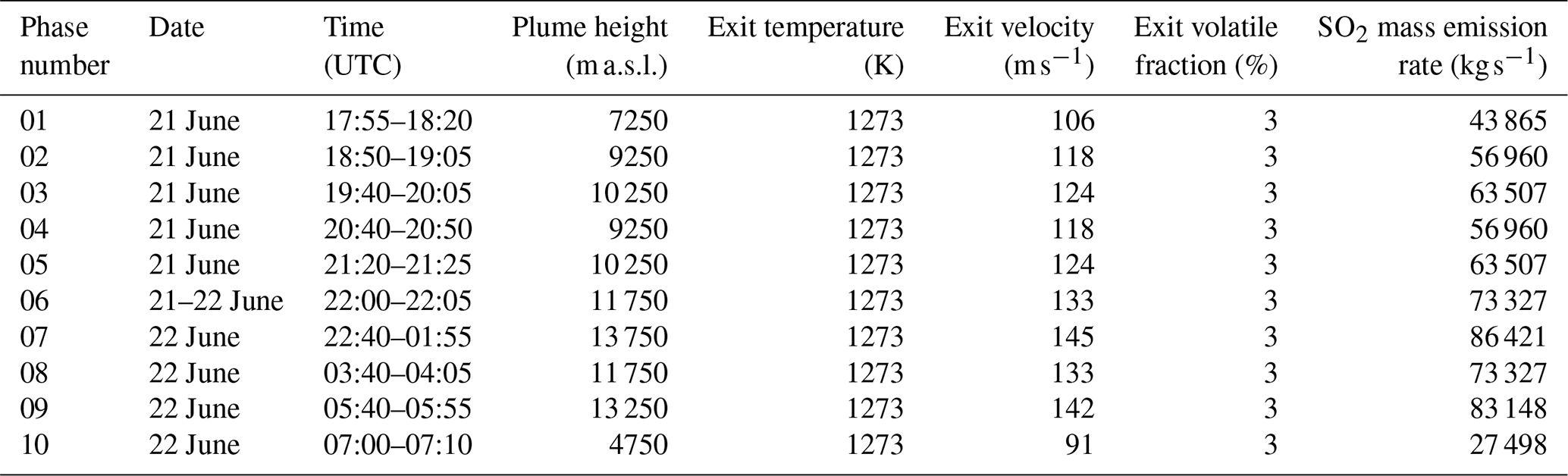
Figure 2 shows the MER of very fine ash that is released into ICON-ART by FPlume (red dots) and the Mastin relationship (blue dots). The fraction of very fine ash relative to the total MER predicted by FPlume is on the order of 1.5 %–3 % (not shown). In most phases, the MER calculated with FPlume is lower than the MER calculated with the Mastin equation, and the difference tends to be higher for larger plume heights. Since the exit parameters are fixed during each phase in the reference case, variation of the MER derived by FPlume must be due to changes in the atmospheric conditions. As the relationship by Mastin et al. (2009) neglects atmospheric conditions and the very fine ash fraction is fixed within one phase, the MERs of the very fine ash are constant within each phase. The vertical profiles of the meteorological variables in Fig. A2a indicate increasing temperatures in most levels below 10 km during the long eruption phase between 9 and 14 h after simulation start. Additionally, the specific humidity increases by up to 1 g kg⁻¹ in the lower 2 km (Fig. A2c). When warmer and moist air is entrained into the plume, the plume density reduces faster due to the lower ambient air density and the release of latent heat. This effect results in a higher positive buoyancy and a lower MER to reach a fixed height. In addition, the wind speed decreases in the lower 4 km between 9 and 14 h after simulation start, which reduces the plume bending, and subsequently the MER needed to reach a fixed height.

According to the MER values in Fig. 2, the total mass of very fine ash emitted in the model for all eruption phases together is about 1.21×10⁹ kg using FPlume and 1.48×10⁹ kg using Mastin-derived MERs.

Figure 2 Mass eruption rate E for very fine ash (t s⁻¹) calculated with the FPlume MER times the very fine ash fraction from Gouhier et al. (2019) (red) and calculated with the Mastin MER times the very fine ash fraction derived in the FPlume experiment (blue). The very fine ash fraction is the same in both experiments to allow for a direct comparison of the FPlume- and Mastin-derived MER on the dispersion in the atmosphere. Active eruption phases are indicated by the gray shading. Please note that the date format in this and following figures is month day, year.

The total mass of very fine ash is evenly distributed as insoluble tracers over the accumulation, coarse, and giant modes. The three insoluble modes are emitted as lognormal distributions with median diameters of 0.8, 2.98, and 11.35 µm, respectively. The standard deviation is 1.4 for each mode.

Following previous studies, we emitted a total of 1.5×10⁹ kg SO₂ (Muser et al., 2020; Kloss et al., 2021; De Leeuw et al., 2021). However, the SO₂ release is linearly adjusted to the eruption heights and length of each phase (Table 1) as follows:

$$\begin{array}{}\text{(3)}& E_{\text{ph}}={\stackrel{\mathrm{‾}}{E}}_{{\mathrm{SO}}_{\mathrm{2}}}\cdot {\displaystyle \frac{H_{\text{ph}}}{H_T}},\end{array}$$

where E_ph is the phase-dependent MER of SO₂, ${\stackrel{\mathrm{‾}}{E}}_{{\mathrm{SO}}_{\mathrm{2}}}$ is the mean MER based on the observed amount of SO₂ and the sum of the duration of all phases, H_ph is the phase plume height (above the vent), and H_T=11 571.2 m is the phase duration-weighted (t) mean plume height derived as

$$\begin{array}{}\text{(4)}& H_T={\displaystyle \frac{{\sum }_{i=\mathrm{1}}^{\mathrm{10}}{H}_{\text{ph},i}\cdot t_i}{{\sum }_{i=\mathrm{1}}^{\mathrm{10}}{t}_i}}.\end{array}$$

Finally, SO₂ release is vertically distributed according to the Suzuki profiles (comparison to previously used profiles in Fig. A1). Here, ICON-ART treats SO₂ as a chemical tracer that can be oxidized by a simplified OH-chemistry scheme as presented in Weimer et al. (2017).

2.5 Himawari-8 ash and SO₂ retrievals

To validate the model results, we used column SO₂ and ash mass loadings estimated from the 16-band visible and infrared Advanced Himawari Imager (AHI) onboard the Himawari-8 geostationary satellite at every full hour. Himawari-8 is operated by the Japan Aerospace Exploration Agency (JAXA) and the Japan Meteorological Agency (JMA). A detailed description of the data product and methods used here is already given in Muser et al. (2020) and references therein. In short, SO₂ is retrieved by the AHI band centered near 7.3 µm, where the absorption of SO₂ is high. A further retrieval scheme, as described in Prata et al. (2004), was applied to minimize the interference with vapor and clouds. For volcanic ash retrievals, the AHI bands near 11.2 and 12.4 µm are considered. The lower detection threshold is <0.2 g m⁻² for volcanic ash. The ash retrievals were corrected by a mask that accounts for pixels that contain meteorological clouds but which were classified as completely cloud covered. Hereby, only pixels inside a 0.1 g m⁻² contour line are considered, and a 9×9 median filter smooths out “spikes”.

2.6 SAL method

The SAL (structure, amplitude, and location) method is an object-based quality measure originally developed to verify precipitation forecasts (Wernli et al., 2008, 2009). However, it has also been successfully applied for transport forecasts of volcanic compounds (e.g., Muser et al., 2020; De Leeuw et al., 2021) and was used in this study for volcanic ash and SO₂ as well. The SAL method evaluates modeled and observed data according to their structure (S), amplitude (A), and location (L). While it assesses predefined objects based on a threshold value for the S and L component, the A component is a normalized domain-averaged quantity. The structure component S compares model and observations with respect to the volume of the defined objects. The value ranges between −2 and 2. Positive values indicate objects that are too large and/or too flat, whereas negative values indicate objects that are too small and/or too peaked. A value of zero refers to a perfect forecast with respect to the structure. The amplitude component A evaluates the domain-averaged relative deviation of the forecasts from observations, and it is positive when the model overestimates the predicted quantity and vice versa (it also ranges between −2 and 2). For a perfect forecast of the amplitude, A is zero. The location component L consists of two parts: L1 describes the agreement between the forecast and observation in terms of the normalized difference between the centers of mass, whereas L2 refers to the average distance between the center of mass of all objects and the individual objects. Both L1 and L2 can reach values between 0 and 1 so that L in total can have values between 0 and 2 with a perfect forecast with respect to the location at L=0 (Wernli et al., 2008, 2009).

For the SAL comparison of Himawari-8 and ICON-ART data, we derived 6 h averages from both datasets at every full hour. Furthermore, we interpolated ash and SO₂ values onto a regular grid at 120^∘ W–80^∘ E and 20–85^∘ N with a resolution of 0.1^∘. However, before interpolation, we applied a 5×5 pixel mean averaging to fill gaps in the mapped satellite data, considering only values different from zero. Otherwise, the linear interpolation would have led to a loss of information when mapping on a coarser grid, because the regular grid is about 4 to 5 times coarser than the retrieval grid. These gaps in the satellite data arise during mapping from the native format onto a regular latitude–longitude grid as needed for the SAL analysis and are due to the increasing pixel sizes towards the edges of the retrieval domain.

To define objects in the SAL analysis, we used a threshold of 0.2 g m⁻² for modeled and observed ash because this is the detection threshold for the Himawari-8 ash retrievals. For SO₂, a threshold of 2.5 g m⁻² for the model and observations is used to remove background SO₂ concentrations in Himawari-8 data. This was necessary because we did not initialize the model with realistic background conditions and, therefore, can only compare the observed and modeled SO₂ plume from the eruption.

3 Results and discussions

3.1 Validation of mass loading

The 2019 Raikoke eruption injected ash and SO₂ up to 14 km into the atmosphere. Figure 3 shows mean ash (left) and SO₂ (right) column on 22 June at 00:00–23:00 UTC (top row) and 23 June at 00:00–23:00 UTC (bottom row) in our reference simulation, FPlume-rad. The volcanic plume first spreads with westerly winds and is then dragged into a low-pressure system over the northern Pacific Ocean. In the mass loadings of both compounds, no clear horizontal separation of the ash and SO₂ plume is visible (compare the left and right sides of Fig. 3). However, we will further investigate the separation of ash and SO₂ due to radiation in Sect. 3.3 after we validated our setup.

Figure 3 Simulated daily mean column mass loadings for ash (a, c) and SO₂ (b, d) on 22 June 2019 at 00:00–23:00 UTC (a, b) and 23 June 2019 at 00:00–23:00 UTC (c, d) (g m⁻²). The results are based on the FPlume-rad experiment.

Figure 4a shows the temporal evolution of the ash loading in the atmosphere following the Raikoke eruption for different experiments and observations. The temporal resolution of the data is 1 h. The Himawari-8 data reveal a steep increase of ash mass at 22:00 UTC on 21 June until a peak of 1.0 Tg is reached at 05:00 UTC on 22 June, and the curve remains above 1.0 Tg for 5 h. The maximum at 07:00 UTC (22 June) of 1.1 Tg is followed by a descent to 0.3–0.5 Tg.

Muser et al. (2020) (green curve) emphasized that aerosol processes account for the ash removal. Nucleation, condensation, and coagulation increase the size of aerosol particles and, thus, lead to a faster sedimentation. However, Muser et al. (2020) were not able to quantitatively explain the time lag between the model and observations during the first hours of the eruption (18:00 UTC on 21 June until 03:00 UTC on 22 June). Besides, the continuous emission with a constant MER led to a slight overestimation of the ash mass loading (Muser et al., 2020). We have closed these gaps as follows.

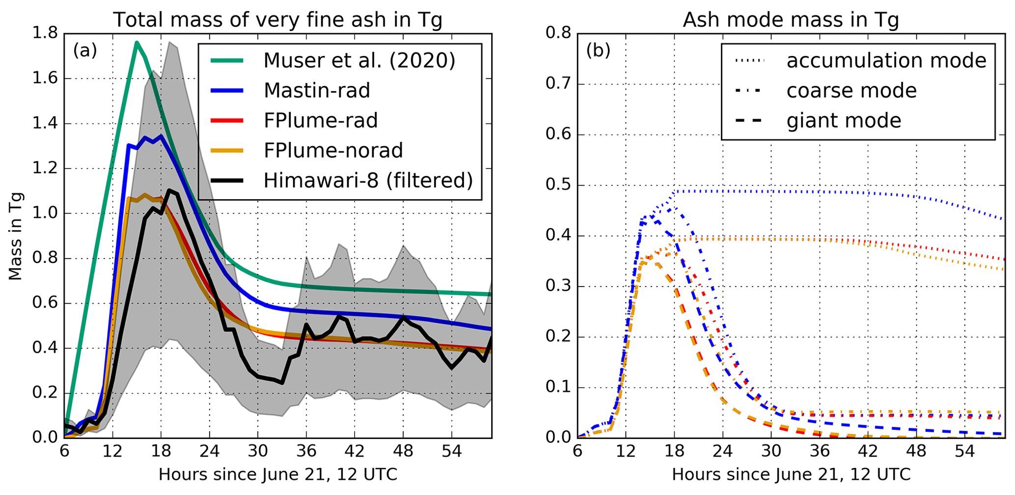
Figure 4 (a) Temporal evolution of the total amount of very fine ash in the atmosphere (Tg) for Himawari-8 observations (black) with an estimated uncertainty range (gray shading). Simulation with one constant emission phase (green, after Muser et al., 2020). Simulation with ICON-ART with and without aerosol–radiation interaction, each with phase-dependent FPlume MERs and a very fine ash fraction derived from the relationship by Gouhier et al. (2019) (red and yellow). Simulation with ICON-ART, eruption-phase-dependent Mastin MERs, and the same very fine ash fraction as for the red curve (blue). (b) Temporal evolution of the simulated mass for the different ash modes (dotted for accumulation modes, dash-dotted for coarse modes, and dashed for the giant mode). The colors refer to the model experiment shown in the panel (a).

The maximum of total ash derived with ICON-ART coupled with FPlume (online treatment) in both experiments with and without radiation–aerosol interaction coincides very well with the Himawari-8 data (in Fig. 4, compare the red and yellow curves with the black curve). The total ash derived with Mastin (a different MER but the same fine ash fractions and emission profile as in the FPlume experiments) overestimates the amount of ash during the first 12 h after the onset of the eruption (blue curve). Thus, neglecting meteorological effects and other plume-related processes in the case of the Raikoke eruption (offline treatment), as is often done in volcanic dispersion forecasts, results in a higher MER especially in the long continuous phase of the eruption and subsequently increased ash emissions into ICON-ART (Fig. 2).

All simulation experiments in Fig. 4a include aerosol dynamics and have correctly reproduced the fallout of particles as indicated by the decrease of ash after 2 d. From Fig. 4b, where the temporal development of the different modes is shown, we can conclude that the decrease of ash after 2 d is mainly due to coarse- and giant-mode particles. The total ash from the simulations with FPlume display the best agreement with the Himawari-8 data in this analysis (Fig. 4a). However, the other curves remain mostly within the error range of Himawari-8 data as well (gray shading). Thus, we conclude that the online treatment of plume development improves the ash loading prediction during the first hours and days after the eruption. After about 30 h, the aerosol dynamical processes become more important, and the differences between the experiments decrease.

3.2 Validation of dispersion using SAL

For the quantitative validation of the forecast quality, we performed a SAL analysis using 6 h averaged SO₂ and ash mass loadings. We compare the results of the FPlume-rad experiment and Himawari-8 satellite data. Figure 5 shows the values for the structure on the abscissa, the amplitude on the ordinate, and the location in colors. We do not discuss the SAL values for the FPlume-norad and the Mastin-rad case here. This is because FPlume-norad only shows very small differences to the FPlume-rad case in all SAL values, and Mastin-rad only changes the amplitude value, as only the MER is higher compared to FPlume-rad. Based on the analysis of hourly to daily mean values, we conclude that 6 h averages provide a reasonable compromise between both reproducing the details and reducing the amount of missing values and noise.

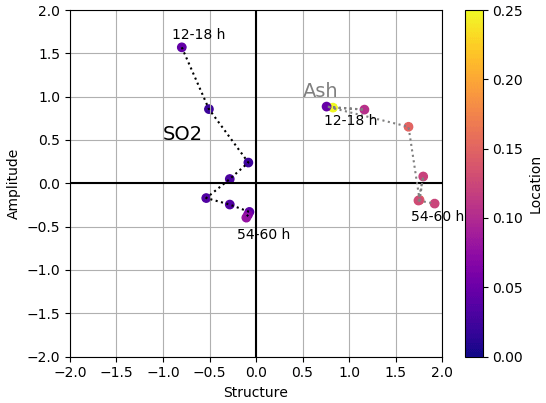
Figure 5 SAL values for ash and SO₂ in the reference experiment (FPlume-rad) with S (structure) on the abscissa, A (amplitude) on the ordinate, and L (location) in colors. The dotted lines connect consecutive hours to visualize the temporal development (black for SO₂ and gray for ash). The labels of the hours are given relative to the start of the simulation on 21 June 2019 at 12:00 UTC.

The location of the SO₂ plume agrees very well between the model and observations throughout the whole simulation period. This is shown by the location values which are close to zero. The structure and amplitude values are close to zero between 24 to 72 h after the beginning of the simulation on 21 June at 12:00 UTC. Thus, there is a high agreement between the model and observations during this period. However, during the first 24 h, the model prediction shows higher amplitude values and a low structure value, indicating a larger mass loading in the model and a less diffuse SO₂ plume in the model compared to the satellite estimates. We argue that the discrepancy in the amplitude between the model and observations during the first hours of the Raikoke eruption stems from the possible underestimation of SO₂ by the satellite retrievals due to the dense ash plume covering the region around the volcano. In addition, our simulation is also affected by the uncertainties of input parameters (e.g., start and end time of individual eruption phases, plume heights, and exit conditions).

The model also predicts the location of the ash plume very well (Fig. 5). The positive structure values indicate that the modeled ash loading becomes more diffusive over the domain for most of the time. Figure A3 (first and second column) compares all 6 h mean ash loadings. The large spread of the modeled ash plume across large parts of the northern Pacific Ocean is not seen in the observations, which is the main reason for the high structure value in Fig. 5. We argue that Himawari-8 measurements of ash at this time might be hampered by water and ice clouds overlapping and obscuring the ash plume. This argument further explains why the temporal evolution of the Himawari-8 measurements in Fig. 4a shows variations between 30 and 60 h, although the emission from Raikoke ceased.

The high amplitude value for ash between 12 and 36 h, despite the almost perfect agreement in the total mass in Fig. 4, also stems from the larger spread of the ash plume in the beginning. The reason is that the background values are considered zero and that the amplitude in the SAL analysis, unlike the object-based structure and location values, is a domain-averaged quantity.

We have shown that the model setup realistically represents the amount of ash following the 2019 Raikoke eruption and that the dispersion of the ash and SO₂ agrees well with the observations. In the next step, we analyze the vertical distribution of the ash and SO₂ plume.

3.3 Vertical separation of the SO₂ and ash plume

In this section, we discuss the evolution of the ash and SO₂ plume top heights and focus on the radiative effects on the plume dynamics.

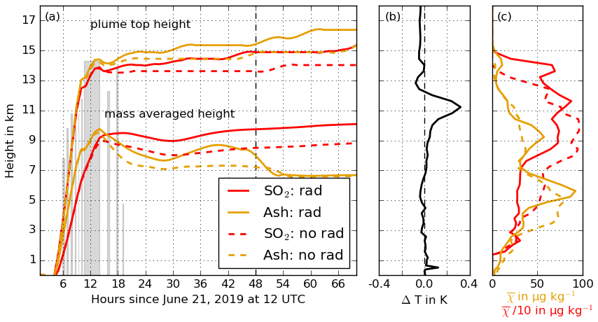
Figure 6 (a) Temporal evolution of the SO₂ (red) and ash (yellow) plume top height and mass-averaged height for the FPlume-rad (solid) and FPlume-norad (dashed) experiment smoothed by a Savitzky–Golay filter. The gray bars indicate the duration and height of the 10 individual eruption phases. They are based on the analysis of the GOES-17 data, which serve as inputs for FPlume. (b) Vertical profile of the temperature difference between FPlume-rad and FPlume-norad in the ash plume 48 h after the start of the simulation. (c) Vertical SO₂ (red) and ash (yellow) profile after 48 h for the FPlume-rad (solid) and FPlume-norad (dashed) experiment.

Figure 6 shows the top height of the ash and SO₂ plume for the FPlume-rad and FPlume-norad experiments (a), the resulting vertical temperature difference on 23 June at 12:00 UTC (b), and the vertical distribution of the SO₂ and ash mixing ratios on the same date (c). The plume top height in (a) is defined as the maximum height of all grid cells in the plume that were separated from background mixing ratios as explained in Sect. 2.2.1. The average plume height in (a) is the mean height weighted by the mass of all grid cells that are considered inside the plume. The values in (b) and (c) were horizontally averaged over the whole detected plume, again excluding grid cells outside the plume. In (b) and (c), we picked 23 June at 12:00 UTC because it allows for a direct comparison to Fig. 8 in Muser et al. (2020), which only shows the ash plume top height. The lines for the plume top height and mass-averaged height are smoothed by a Savitzky–Golay filter to remove “steps” due to the low vertical resolution at upper-atmospheric model levels. The difference in height between FPlume-rad and FPlume-norad remains similar, regardless of the use of this filter. However, the increasing plume height already starting before the beginning of the eruption is a result of the filtering.

During the first hours after the beginning of the eruption, the plume top height for ash and SO₂ mainly rises due to the higher eruption heights of later eruption phases. The gray bars, which indicate the eruption height, coincide well with the top height (Fig. 6a).

Shortly after the end of the long eruption phase, we clearly see a separation of the ash plume top height between the FPlume-rad and the FPlume-norad experiments. The effect of the ash lofting due to radiation was already investigated in detail by Muser et al. (2020) with the same model system. They found that the absorption of shortwave and longwave radiation by the coated ash particles leads to the warming and rising of the ash plume. We compare the vertical profile of the temperature difference between the FPlume-rad and FPlume-norad cases here with the vertical temperature differences in Muser et al. (2020) on 23 June at 12:00 UTC. A single large positive anomaly of approximately 0.3 K near 11 km occurs in our simulation (Fig. 6b). Subsequently, the whole ash plume rises to higher altitudes. In contrast, Muser et al. (2020) found two distinct temperature anomaly peaks around 10 and 14 km on the order of 0.25 K each, which result in the formation of two maxima in the ash mixing ratios near 10 and 15 km. The resulting uplift during the first 12 h in the ash plume in our simulation is about 33 % of the resulted lifting in Muser et al. (2020).

In the first hours during and after the eruption, the absorption-induced warming of the ash plume also causes the SO₂ plume to rise in FPlume-rad (Fig. 6a and c). However, as SO₂ itself absorbs neither solar nor terrestrial radiation in our model setup, the ash plume top height clearly separates from the SO₂ plume top height with increasing time (Fig. 6a). The vertical profiles of the SO₂ mixing ratio in the FPlume-rad and FPlume-norad cases indicate that radiation interaction smooths and reduces the vertical gradient of the SO₂ mixing ratios in the troposphere. In the stratosphere, a second peak occurs above the maximum emission height (Fig. 6c).

The evolution of the mass-averaged height of the ash and SO₂ plume indicates behavior opposite to that of the plume top height. The mass average of the SO₂ plume is generally higher than for the ash plume. In Fig. 7a and c, the vertical distribution of the ash and SO₂ mass concentrations (kg m⁻³) confirm that the SO₂ plume is about 5 km higher on average than the ash plume after 3 d. This is in agreement with several existing studies (e.g., Timmreck, 2012; Robock, 2000), which emphasized a fast removal of ash after volcanic eruptions related to the higher weight of ash particles compared to SO₂. The stepwise reduction of the ash in the mass-averaged height is related to the loss of the giant mode during the first 24 h and the large fallout of the coarse mode until about 50 h relative to simulation start (Figs. 4b and A4).

Figure 7 (a, c) Temporal evolution of the horizontally averaged vertical distribution of ash mass concentration (a) and SO₂ mass concentration (c) in the FPlume-rad experiment. (b, d) Number-weighted characteristic ash radius (Eq. 5) for FPlume-rad (b) and difference between FPlume-rad and FPlume-norad (d).

In the next step, we want to compare the vertical distribution of a characteristic ash particle radius $\stackrel{\mathrm{‾}}{R}$, which we calculated as follows:

$$\begin{array}{}\text{(5)}& \stackrel{\mathrm{‾}}{R}={\displaystyle \frac{{\sum }_{i=\mathrm{1}}^{\mathrm{5}}{r}_{\mathrm{m},i}\cdot N_i}{{\sum }_{i=\mathrm{1}}^{\mathrm{5}}{N}_i}}.\end{array}$$

For the overall characteristic radius $\stackrel{\mathrm{‾}}{R}$, we consider the five ash modes $i=\mathrm{1},\mathrm{5}$ (insoluble and mixed accumulation modes, insoluble and mixed coarse modes, and giant mode) and calculated $\stackrel{\mathrm{‾}}{R}$ at every grid cell. r_m is the median radius from the lognormal distribution, and N is the number of particles per grid box. The vertical distribution of the horizontally averaged characteristic radius in Fig. 7b also shows the loss of the larger particles (coarse and giant modes) during the first 24 h. Afterwards, the values of the mean characteristic radius are below 1.5 µm with a maximum around 5 to 6 km. In comparison to the FPlume-norad experiment, the characteristic radius is higher on average compared to the FPlume-rad experiments because aerosol–radiation interaction slows down the removal of larger particles from the atmosphere (Fig. 7d). This effect is visible in the removal of the accumulation mode, which is reduced in FPlume-rad (Fig. 4b). Compared to FPlume-norad, the removal of the coarse modes in FPlume-rad is delayed by about 1 h between 18 and 25 h after simulation start (Fig. 4b). After about 30 h the amount of the coarse mode is slightly lower in FPlume-rad than in FPlume-norad because the particle radius is larger at most altitudes (Figs. 4b and 7d). The temporal removal of the giant mode only shows small differences between FPlume-rad and FPlume-norad (Fig. 4b). The larger mean characteristic radius after approximately 48 h is related to an increasing removal of accumulation mode particles in FPlume-norad compared with FPlume-rad (Figs. 7d and 4b). However, we will leave a detailed analysis of the processes changing particle radii to further work.

Both the main SO₂ mass and the main ash mass are restricted to a narrower vertical range after 3 simulation days compared to the end of the eruption (around 13 h after simulation start). The location of the SO₂ is between 8 and 14 km and between 4 and 7 km for ash (Fig. 7). Thus, for initializing long-range and climate simulations, a release of SO₂ and ash at these altitudes is justified if the sedimentation during the first hours is considered in the total emission rate.

Despite the clear vertical separation of the ash and SO₂ plume, the horizontal separation in both model and observations remains small in the first 3 d after the eruption. Nevertheless, a strong vertical wind shear can result in the horizontal separation of the ash and SO₂ plume on longer timescales as in Kloss et al. (2021).

4 Conclusions

We investigated the 2019 Raikoke eruption, which was characterized by nine shorter eruption phases and one continuous eruption phase of almost 3 h duration. Here, we describe a model setup in which the ESPs were improved by (1) coupling ICON-ART with FPlume to account for the effect of changing volcanic and meteorological conditions and (2) a delineation of eruption phases. We further investigated the effect of radiation–aerosol interaction on the SO₂ plume due to a warming of the ash plume. The main findings are the following.

1. We demonstrated a large improvement of the total ash burden forecast in the first 12 h by resolving the individual eruption phases of the Raikoke eruption, which reduces the ash mass overestimation from 37 % to 18 %. Additionally, the online calculation of ESPs by FPlume further improves temporal evolution of the simulated ash mass, which shows an almost perfect agreement with the observed evolution of ash mass loading.

2. In addition to the mass loading, the predicted spatial dispersion of the ash and SO₂ plume also agrees well with observations from Himawari-8 as our SAL analysis reveals. However, we hypothesize that the validation of the simulated ash and SO₂ dispersion is partially hampered by a dense ash plume in the beginning of the eruption and by overlapping water and ice clouds later on.

3. As already demonstrated in Muser et al. (2020), aerosol–radiation interaction leads to a warming of the volcanic ash plume and, therefore, to a lofting of ash particles during the first hours. Here, we additionally found a lofting of the SO₂ plume during the first 12 h after the eruption caused by a warming of the plume. However, with increasing time, the SO₂ plume becomes more and more vertically separated from the ash plume, and the lofting slows down. This is related to a faster sedimentation of the ash particles compared to SO₂ and the fact that SO₂ does not absorb solar radiation in our model.

Appendix A

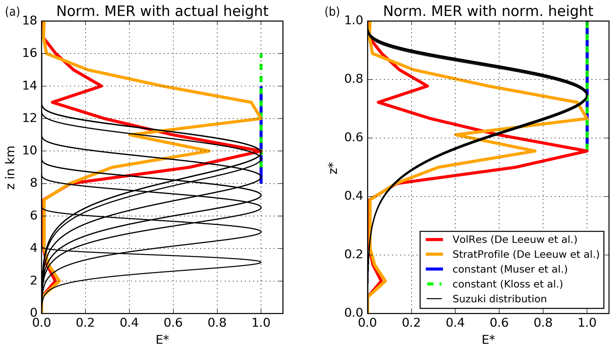
Figure A1 Comparison of the Suzuki profiles used in this work with vertical emission profiles from previous studies (“VolRes” and “StratProfile” from De Leeuw et al., 2021, and constant profiles from Muser et al., 2020, and Kloss et al., 2021). (a) Normalized with respect to the MER (E^∗) but with actual emission heights (z). (b) Normalized with respect to the MER and emission height (z^∗).

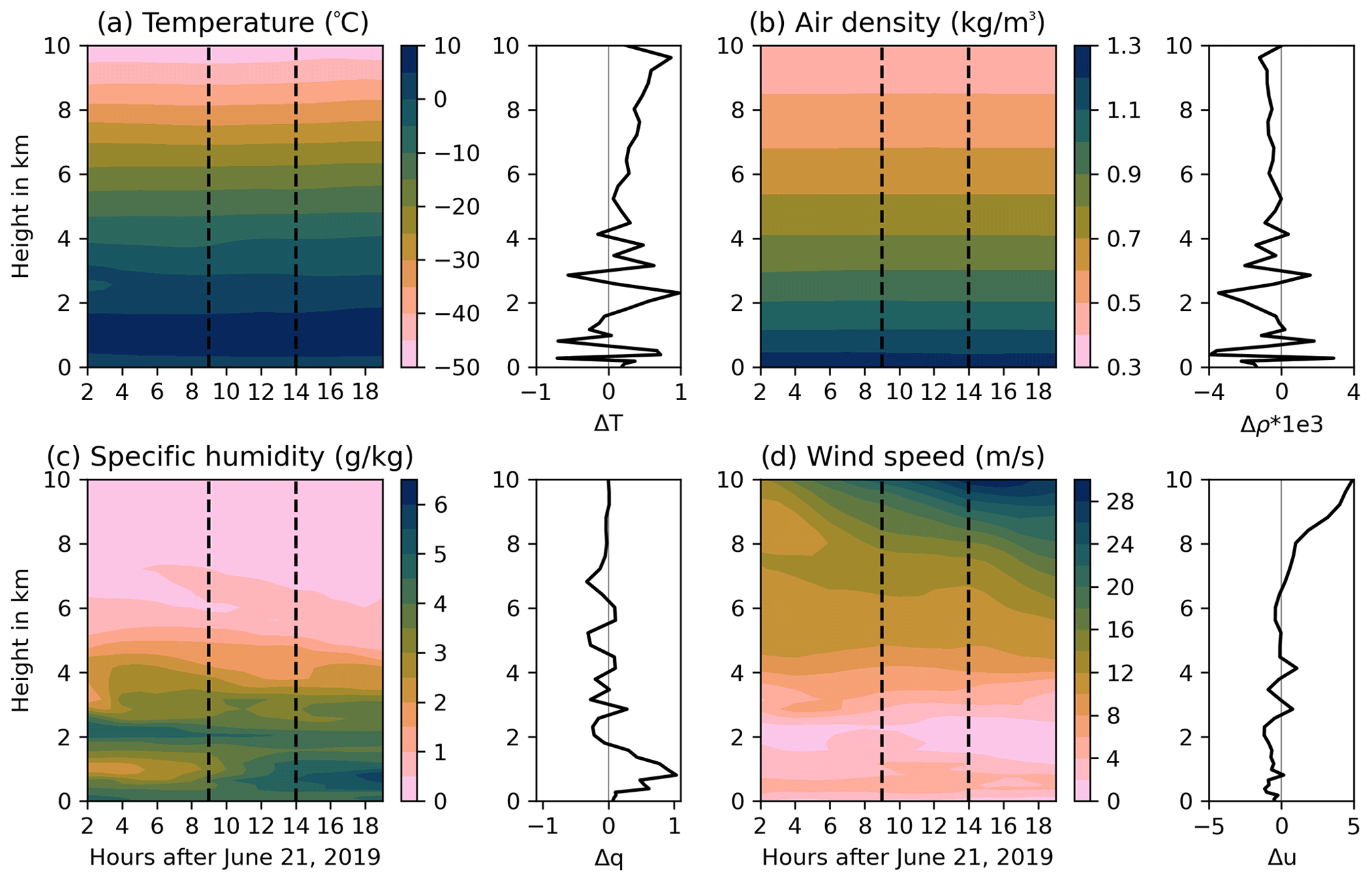
Figure A2 Meteorological conditions above the vent in the first 20 h after simulation start to explain variations in the FPlume-derived MER. Four different atmospheric variables are shown: (a) temperature (^∘C), (b) air density (kg m⁻¹), (c) specific humidity (g kg⁻¹), and (d) wind speed (m s⁻¹). For each variable the temporal development in the vertical axis above the vent is given over time in contours and the difference between the two time steps indicated by the vertical dashed lines in the contour plot (later step minus earlier time step).

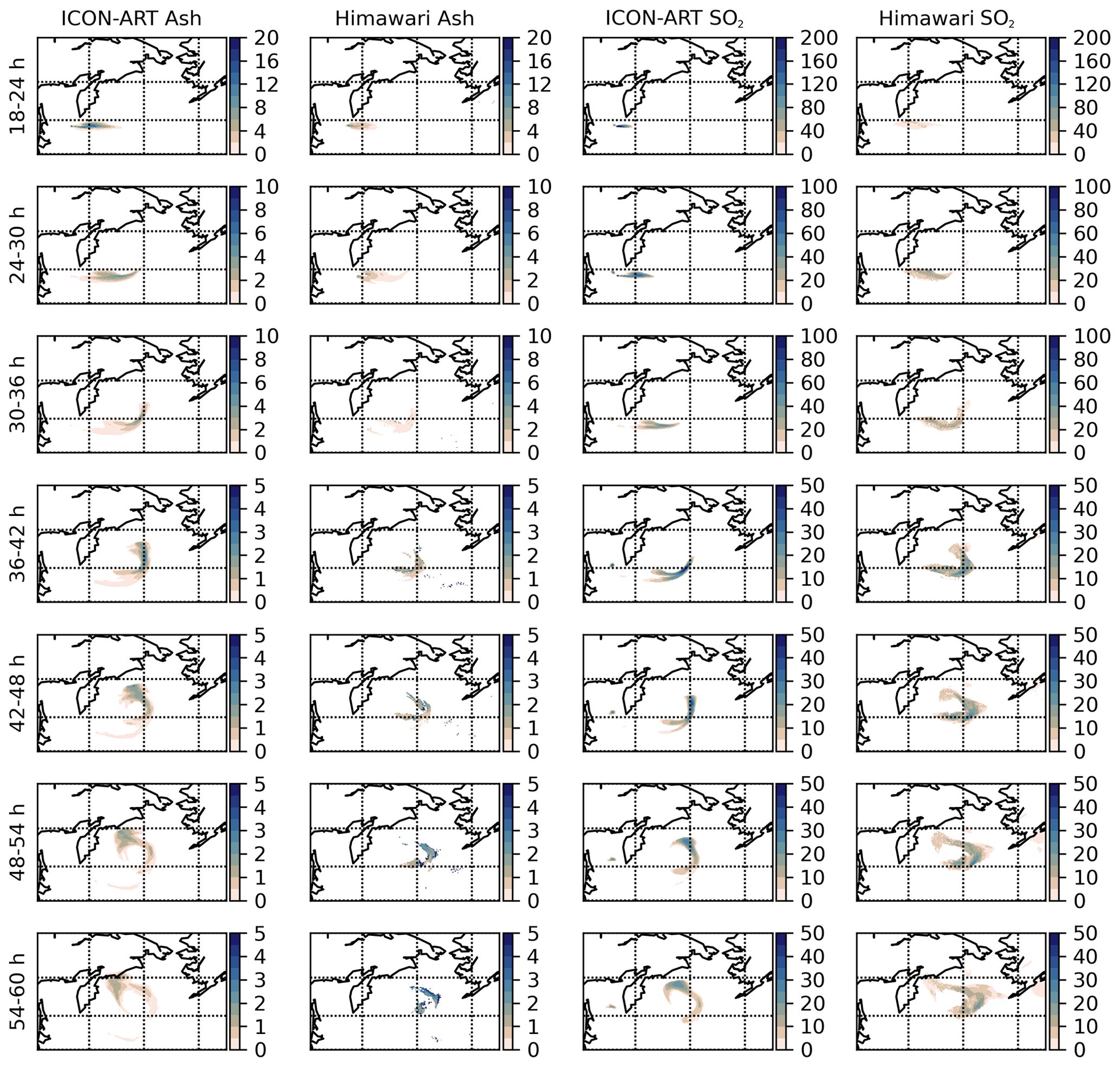
Figure A3 Comparison plots for seven ash and SO₂ 6 h averaged column loadings (row 1 to 7) in order to explain the discrepancy between simulated ICON-ART data and Himawari-8 observed data in the SAL analysis. First and second column: ash column loadings (g m⁻²) from ICON-ART and Himawari-8. Third and fourth column: SO₂ column loadings (g m⁻²) from ICON-ART and Himawari-8.

Figure A4 Horizontally averaged ash particle characteristic radius of the lognormal distribution (µm) (left, Eq. 5) and horizontal sum of the particle number (right) of the different ash modes: insoluble accumulation (a, b), mixed accumulation (c, d), insoluble coarse (e, f), mixed coarse (g, h), and giant (i, j).