the Creative Commons Attribution 4.0 License.
the Creative Commons Attribution 4.0 License.
 | 15 Mar 2022
Interpreting machine learning prediction of fire emissions and comparison with FireMIP process-based models
Yun Qian
Yang Zhang
Annual burned areas in the United States have increased 2-fold during the past decades. With more large fires resulting in more emissions of fine particulate matter, an accurate prediction of fire emissions is critical for quantifying the impacts of fires on air quality, human health, and climate. This study aims to construct a machine learning (ML) model with game-theory interpretation to predict monthly fire emissions over the contiguous US (CONUS) and to understand the controlling factors of fire emissions. The optimized ML model is used to diagnose the process-based models in the Fire Modeling Intercomparison Project (FireMIP) to inform future development. Results show promising performance for the ML model, Community Land Model (CLM), and Joint UK Land Environment Simulator-Interactive Fire And Emission Algorithm For Natural Environments (JULES-INFERNO) in reproducing the spatial distributions, seasonality, and interannual variability of fire emissions over the CONUS. Regional analysis shows that only the ML model and CLM simulate the realistic interannual variability of fire emissions for most of the subregions (r>0.95 for ML and for CLM), except for Mediterranean California, where all the models perform poorly (r=0.74 for ML and r<0.30 for the FireMIP models). Regarding seasonality, most models capture the peak emission in July over the western US. However, all models except for the ML model fail to reproduce the bimodal peaks in July and October over Mediterranean California, which may be explained by the smaller wind speeds of the atmospheric forcing data during Santa Ana wind events and limitations in model parameterizations for capturing the effects of Santa Ana winds on fire activity. Furthermore, most models struggle to capture the spring peak in emissions in the southeastern US, probably due to underrepresentation of human effects and the influences of winter dryness on fires in the models. As for extreme events, both the ML model and CLM successfully reproduce the frequency map of extreme emission occurrence but overestimate the number of months with extremely large fire emissions. Comparing the fire PM2.5 emissions from the ML model with process-based fire models highlights their strengths and uncertainties for regional analysis and prediction and provides useful insights into future directions for model improvements.
- Article
(14300 KB) - Full-text XML
-
Supplement
(2749 KB) - BibTeX
- EndNote


Large fires have increased across the United States over the past 2 decades, especially in the western US. While the total area burned in 2020 increased by 51 % compared to the 10-year average for 2010–2019, the total number of fires in 2020 is smaller than the 10-year average. This indicates the contribution of larger and more powerful fires to the growing burned areas (NIFC, 2020). Large fires can directly lead to property damage and pose a threat to human lives (Thomas et al., 2017). Meanwhile, fine particulate matter (PM2.5, particles with an aerodynamic diameter smaller than and equal to 2.5 µm) emitted from fires not only have negative impacts on human health but also affect climate and ecosystems (Johnston et al., 2012; Ward et al., 2012; Rap et al., 2013; Kaulfus et al., 2017; Liu et al., 2018; Wang et al., 2018; Stowell et al., 2019). Driven by stronger fire heating and with higher injection height, aerosols emitted from large fires can be transported to broader area and stay in the atmosphere longer. Given the increasing trend of fire emissions, fire smoke may become the predominant source of PM2.5 in the US in the future (Yue et al., 2013; Liu et al., 2016; Ford et al., 2018). Thus, an accurate prediction of fire emissions is imperative for investigating the impacts of historical and future fires on air quality, human health, and climate.
One of the widely used methods for predicting fire emission is process-based fire parameterization. These process-based models generally employ universal functions depicting non-linear relationships between fires and the input variables and apply the same functions to all grid cells in a model (Pechony and Shindell, 2009; Thonicke et al., 2010). In addition, the parameters of the process-based model are usually determined by empirical or statistical functions, assuming that the same parameters apply to all the regions or regions with limited fire observations (Crevoisier et al., 2007; Parisien et al., 2016). Recently, Zou et al. (2019) developed the Region-Specific ecosystem feedback Fire (RESFire) model that includes region- and PFT-specific fire parameterizations in subregions over the globe. Their model shows improved spatial distributions and temporal variations in fire activities compared to the CLM fire model. Process-based models are usually included in the dynamic global vegetation models (DGVMs) to simulate fire dynamics, vegetation dynamics, and biogeochemistry driven by atmospheric forcing and socio-economic data (Li et al., 2013; Knorr et al., 2016). Fire emissions, including trace gases and aerosols, are calculated from the simulated fire carbon emissions and the emission factors, with the former computed as the product of the burned area, fuel load, and combustion completeness. The process-based models in DGVM coupled with other components of Earth system models can be used to assess the impacts of environmental factors on fires and the feedback between fire emissions, land processes, and climate (Kloster et al., 2010). In 2014, the Fire Model Intercomparison Project (FireMIP) was initiated to compare nine DGVMs that include fire modules to better understand the performances of the global fire models (Rabin et al., 2017). FireMIP enables comprehensive evaluation and comparison across various process-based models and provides a dataset of long-term fire simulations for regional and global analysis (Li et al., 2019a; Hantson et al., 2020).
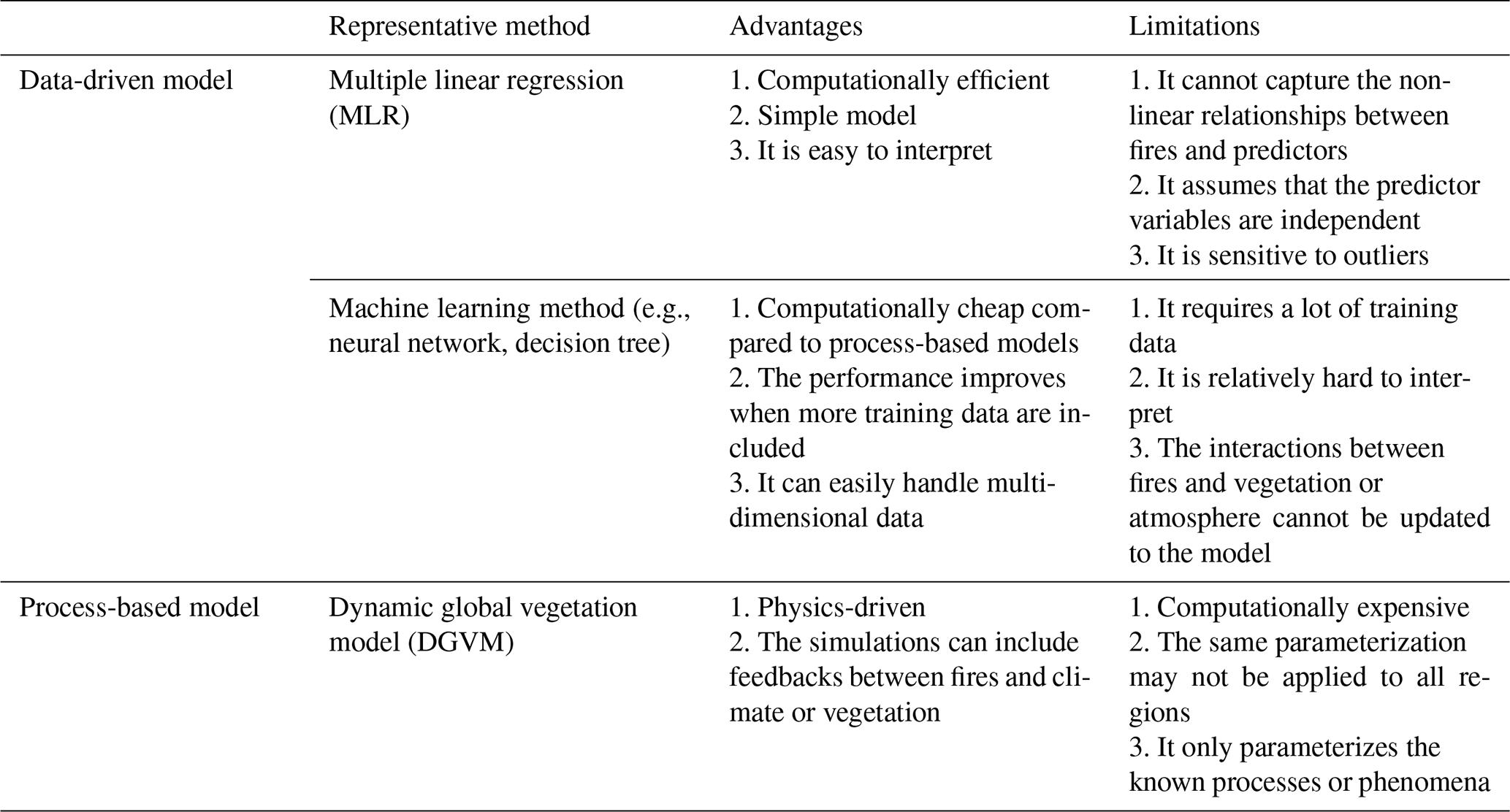
Besides process-based fire models, data-driven statistical models are also commonly used to estimate fire activities using relationships between fires and predictor variables. Multiple linear regression (MLR) is a popular simple statistical method used for fire modeling (Spracklen et al., 2009; Morton et al., 2013; Urbieta et al., 2015; Williams et al., 2019). MLR can achieve a good performance, but it fails to capture the non-linear relationships between fires and predictors, and it is sensitive to the collinearity and combinations of predictors (Littell et al., 2009). Unlike MLR, machine learning (ML) is a novel tool for advancing fire modeling, given its strengths in resolving the complex relationships between the target and predictor variables. Different ML approaches have been used to estimate fire occurrence, burned areas, or emissions at various timescales and spatial scales (Cortez and Morais, 2007; Aldersley et al., 2011; Dillon et al., 2011; Birch et al., 2015; Kane et al., 2015; Coffield et al., 2019; Wang and Wang, 2020). Even though ML models generally achieve higher accuracy than simple statistical models, their decision processes are often inscrutable and hence lack interpretability. The development of explainable ML represents major advances for scientific applications beyond predictions (Gunning, 2019; Arrieta et al., 2020). For example, Wang et al. (2021a) used the extreme gradient boosting (XGBoost) algorithm and Shapley additive explanation (SHAP) to predict wildfire-burned area and revealed the relationships between burned areas and predictor variables. As process-based and data-driven models have their own advantages and weaknesses, as listed in Table 1, comparing these models and assessing their uncertainties in historical simulations and future projections are important. Yue et al. (2013) applied an MLR and a parameterization method to estimate burned areas in ecoregions of the western US and found that both models explained ∼ 50 % of the variance in the observed burned areas. Although they compared the burned areas estimated by the two methods and quantified their uncertainties in fire projections, both methods are only driven by meteorology while the effects of fuels and human activities are not considered.
Table 1Advantages and limitations of different types of fire models.
The FireMIP dataset provides long-term simulations of multiple DGVMs with fire modules, allowing comparisons between process-based and data-driven models, with all models considering all the potential factors influencing fires, including climate, weather, vegetation, and human activities. This study aims to develop an ML model with game theory interpretation for fire emission prediction and to understand controls of fire emissions. The ML model and SHAP are then used to reveal the important factors controlling fire emissions and diagnosis of the process-based FireMIP models. The ML model predicts the monthly PM2.5 emissions from fires during 2000–2020 at a spatial resolution of over the contiguous US (CONUS). It uses the XGBoost algorithm and incorporates various predictors, including local and large-scale meteorology, land surface characteristics, and socioeconomic variables, which are common input variables also used by the FireMIP models while some are specifically related to fire activities in the CONUS. We acknowledge that different input variables between the ML and FireMIP models might cause additional uncertainty for comparison. This study aims to construct an ML model that predicts fire emissions over the CONUS and utilizes the ML model and SHAP to reveal the important factors contributing to fire emissions that might not be fully represented in the process-based models. In this context, the ML model and FireMIP models are optimized using different data or predictors at various scales, which enables us to use the ML to diagnose the performance of FireMIP models over the CONUS through the comparisons of their performances and variable importance from the ML model. We evaluate and compare the predicted fire emissions from the ML and FireMIP models against the GFED fire emission product, focusing on spatial distributions, seasonality, and interannual variability over selected regions in the CONUS. Additionally, the ML model and the SHAP importance are used to identify the important drivers of fire emissions in different regions and compare them with the corresponding parameterizations in the process-based models. Lastly, we compare the process-based and ML model performances in simulating extremely large fire emissions, including the spatial distributions of frequency and two case studies.
2.1 Fire-induced PM2.5 emission data
Monthly fire PM2.5 emission data are obtained from the Global Fire Emissions Database (GFED). GFED version 4 provides monthly burned area at 0.25∘ spatial resolution from 1997 to present, based on a combination of the MODIS burned area product with active fire data from the Tropical Rainfall Measuring Mission (TRMM), Visible and Infrared Scanner (VIRS), and Along-Track Scanning Radiometer (ATSR) family of sensors (Giglio et al., 2013). The GFED fire PM2.5 emissions are estimated by combining the burned area boosted by small fires (Randerson et al., 2012) and the emission factors based on Akagi et al. (2011) with a revised version of the Carnegie-Ames-Stanford Approach (CASA) biogeochemical model that estimates fuel loads and combustion completeness for each monthly time step (van der Werf et al., 2017). The emission factors are dependent on the fire types, including savanna, boreal forest, temperate forest, tropical forest, and agriculture (van der Werf et al., 2017). We use the GFED fire PM2.5 emission as the target variable in the machine learning model development and for model evaluation.
To reduce spatial heterogeneity and help model learning, we apply the inverse distance weighting (IDW) (Bartier and Keller, 1996; Shepard, 1968) to interpolate the monthly gridded fire PM2.5 emission at . The IDW method determines the value at a grid cell as the weighted average of the surrounding values within a search distance, with the weights proportional to the inverse of the distance raised to the power value p. Here we choose a value of 1 for p and a search distance of 35 km for IDW processing. Note that the total fire-emitted PM2.5 within a search distance after IDW processing is constrained to be the same as the original data. In this study, we only include grids with more than 8 months of fire emissions larger than zero (in a total of 250 months), encompassing 90 % of the total fire emissions and ensuring sufficient data for the XGBoost model training. The interpolated fire emission is normalized based on its 21-year mean and standard deviation for each grid to reduce the skewness and improve data symmetry.
2.2 Predictor variables
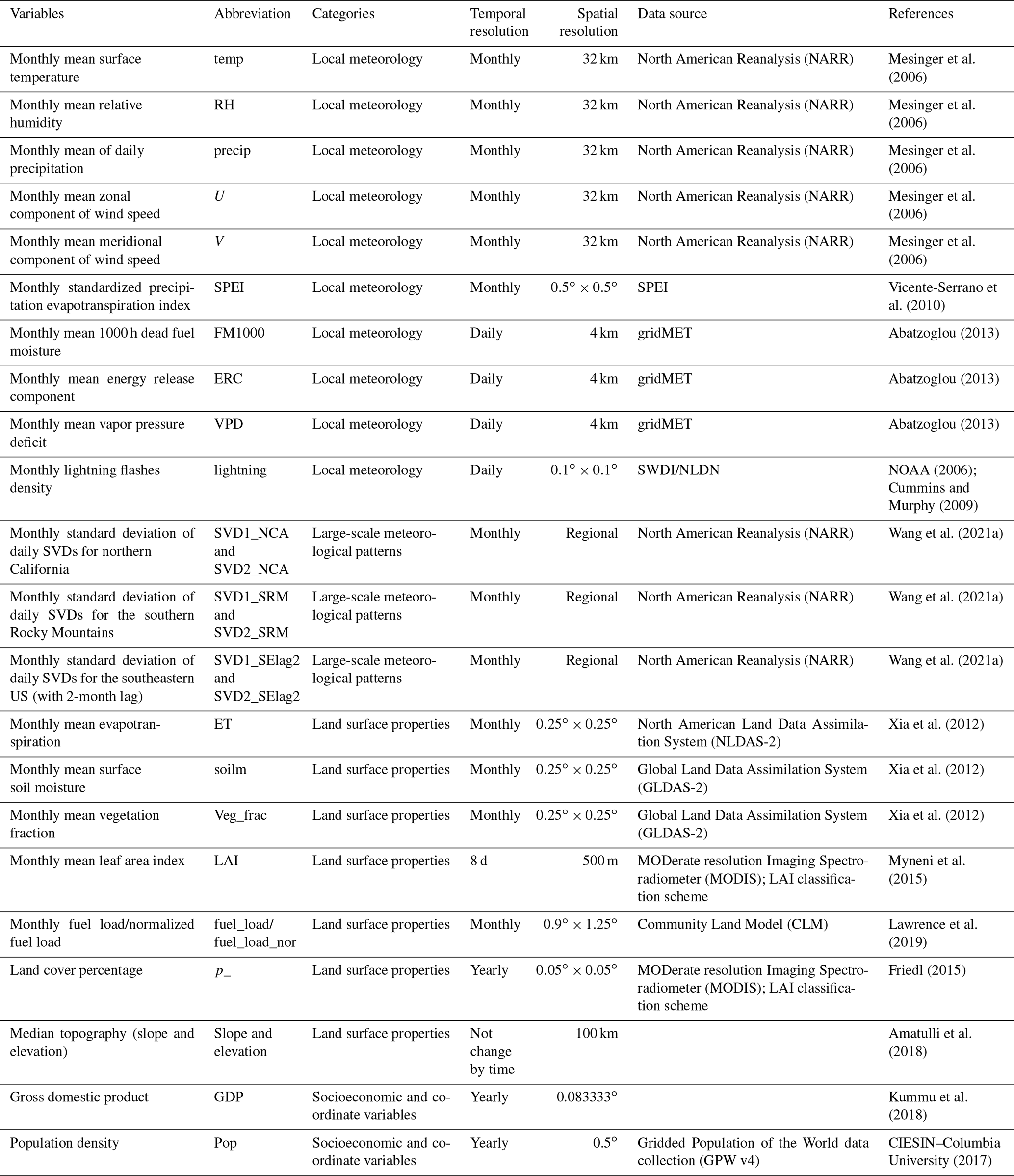
We develop an empirical model at grid resolution driven by various predictor variables at a monthly scale from January 2000 to October 2020. Given the fact that the datasets have different spatial resolutions, all the predictor variables are resampled to the spatial resolution of by linear interpolation. The predictor variables used in the model along with their original spatial and temporal resolutions are included in Table 2. Most variables were also used in Wang et al. (2021a) for developing an ML model of fire-burned area over the contiguous US.
2.2.1 Local meteorology
The same as the local meteorological predictors used in Wang et al. (2021a), we include monthly data of mean surface temperature, relative humidity (RH) at 2 m, daily precipitation, zonal (U) and meridional (V) components of wind at 10 m from the North American Regional Reanalysis (NARR) (Mesinger et al., 2006), and 1000 h dead fuel moisture (FM1000), energy release component (ERC), and vapor pressure deficit (VPD) from the gridMET dataset (Abatzoglou and Kolden, 2013; Coffield et al., 2019). Drought is a natural phenomenon that influences fires through ignition efficiency, fuel availability, and fuel moisture. Thus, we include the monthly standardized precipitation evapotranspiration index (SPEI), a multiscalar drought index based on climatic data (Vicente-Serrano et al., 2010). Given that lightning is one of the major ignition sources of fires and makes up approximately 75 % of burned areas in western US (Pyne, 1984; Stephens, 2005), in this study, we add the cloud-to-ground (CG) lightning flash density from Severe Weather Data Inventory (SWDI) based on the National Lightning Detection Network (NLDN) (Cummins and Murphy, 2009; NOAA, 2006). The daily number of CG lightning flashes is summarized in 0.1∘ tiles, and we aggregate the daily data to a monthly scale.
2.2.2 Large-scale meteorological patterns
Large-scale meteorological patterns at a synoptic scale have been linked to large fire events (Crimmins, 2006; Trouet et al., 2009; Zhong et al., 2020; Dong et al., 2021). Furthermore, it has been shown that including predictors of large-scale meteorological patterns conducive to wildfires significantly improves the prediction of burned areas over the CONUS (Wang et al., 2021a). Thus, we follow the methods developed by Wang et al. (2021a) using the singular value decomposition (SVD) method to construct predictors representing the synoptic patterns driving fire emission variability. Note that the only difference between Wang et al. (2021a) and this study is that they used wildfire-burned-area data and we use fire emissions to construct the SVDs. Three regions where large fires periodically occur are selected for constructing SVDs: northern California, the southern Rocky Mountains, and the southeastern US, as defined in Wang et al. (2021a). For each region, we calculate the daily mean fire PM2.5 emissions over the region and compute the day-to-day correlations between the regional mean fire PM2.5 emissions and the five gridded daily meteorological variables (surface temperature, 2 m RH, U wind and V wind at 850 hPa, and geopotential height at 500 hPa) for all grid cells within the large-scale domain, giving a correlation map for each meteorological variable. The correlation maps are then used to derive the SVD modes representing the large-scale meteorological patterns related to fires. Finally, we compute the monthly standard deviation of the daily SVD time series for the first two SVD modes, representing the month-to-month variations of synoptic fluctuations and atmospheric instability. The detailed methods and discussions about the SVDs are provided in Wang et al. (2021a). Overall, the identified SVDs for the three regions are similar to the SVDs in Wang et al. (2021a) calculated using wildfire-burned areas (Figs. S1–S3 in the Supplement).
2.2.3 Land surface properties
We use the same set of variables in the burned-area model that represent the effects of fuel and land surface states on fire emissions, including evapotranspiration (ET), surface soil moisture, land types, and topography (Wang et al., 2021a). Monthly mean ET, vegetation fraction, and surface soil moisture are obtained from the North American Land Data Assimilation System (NLDAS-2) (Xia et al., 2012). Land cover data of the LAI classification scheme are obtained from the Terra and Aqua combined MODIS Land Cover Climate Modeling Grid (CMG) version 6 data (Friedl, 2015). Since the land cover data are at yearly intervals from 2001 to 2020, we use the land cover data of 2001 for 2000. Topography data of slope and elevation are obtained from Amatulli et al. (2018).
Besides the above-mentioned variables that were also used in Wang et al. (2021a), in this study, we consider the effect of fuel load on fire emissions, since fuel load is critical to fire emissions through its controls on fuel consumption and burned areas (Parks et al., 2012; Liu and Wimberly, 2015). As there are limited observations of fuel load, we use LAI to approximate the canopy bulk density, which is an important crown characteristic to predict crown fire spread, and vegetation fraction to represent the existing amount of vegetation (Keane et al., 2005). LAI is taken from MODerate resolution Imaging Spectroradiometer (MODIS) instruments (Myneni et al., 2015), and vegetation fraction is obtained from the NLDAS-2. As LAI may not fully represent the available biomass, we also include fuel load simulated by the Community Land Model (CLM). Monthly fuel load data from 2000 to 2015 are obtained from a simulation by CLM version 5 with biogeochemistry and prognostic crop, driven by atmospheric forcing from GSWP3v1 (Lawrence et al., 2019). The fuel load after 2015 is taken from a simulation under the SSP3 (shared socioeconomic pathways) scenario. CLM fuel load is validated by comparing with the fuel-measured fuel load from the global fuel consumption database (van der Werf et al., 2017; van Leeuwen et al., 2014), as shown in Fig. S4. The CLM-simulated fuel load is generally consistent with the measured fuel load for different vegetation types across the CONUS based on the limited measurements. Additionally, we include normalized fuel load as a predictor to capture the effects of temporal variation in fuel load, as the influence of fuel load on fire emissions is mainly attributed to its spatial variation rather than the temporal variation (Lasslop and Kloster, 2015).
2.2.4 Socioeconomic variables
We use population density and gross domestic product (GDP) per capita to represent human effects on wildfires. The population density data are obtained from the Gridded Population of the World (GPW V4) data collection for the years 2000, 2010, 2015, and 2020, with a spatial resolution of 30 arcsec (CIESIN, 2017). The populations in other years are linearly interpolated between the abovementioned four years. The GDP per capita is taken from a gridded global dataset for 2000–2015 with a spatial resolution of 5 arcmin (Kummu et al., 2018). For the GDP after 2015, we use the data of 2015.
3.1 Process-based fire emission models
The Fire Model Intercomparison Project (FireMIP) includes a set of common fire modeling experiments from nine DGVMs driven by the same forcing data, allowing a better understanding of global fire models (Rabin et al., 2017). The FireMIP dataset provides global gridded burned area fraction and fire emissions, including carbon and 33 species of trace gases and aerosols over 1700–2012. Nine DGVMs with different fire modules are included in FireMIP, including Community Land Model version 4.5 (CLM4.5) with the CLM5 fire module, Canadian Terrestrial Ecosystem Model (CTEM), Jena Scheme for Biosphere-Atmosphere Coupling in Hamburg with Spread and InTensity fire model (JSBACH-SPITFIRE; hereafter referred to as JSBACH), Joint UK Land Environment Simulator with Interactive Fire And Emission Algorithm For Natural Environments (JULES-INFERNO; hereafter referred to as JULES), Lund-Potsdam-Jena General Ecosystem Simulator with Global FIRe Model (LPJ-GUESS-GlobFIRM; hereafter referred to as LPJ-Glob), LPJ-GUESS with SIMple FIRE model and Blaze-Induced Land-Atmosphere Flux Estimator (LPJ-GUESS-SIMFIRE-BLAZE; hereafter referred to as LPJ-SIM), LPJ-GUESS with SPITFIRE model (LPJ-GUESS-SPITFIRE; hereafter referred to as LPJ-SPI), MC2, and Organizing Carbon Hydrology In Dynamic Ecosystems with SPITFIRE model (ORCHIDEE-SPITFIRE; hereafter referred to as ORCHIDEE) (Rabin et al., 2017).
The nine DGVMs in FireMIP are driven by the CRU-NCEP v5.3.2 atmospheric forcing data with a spatial resolution of 0.5∘ and a 6-hourly temporal resolution (Wei et al., 2014; Rabin et al., 2017). Other forcing data, including annual global atmospheric CO2 concentration, land use and land cover, and population density from 1700 to 2012, are taken from various data sources (Klein Goldewijk et al., 2010; Hurtt et al., 2011; Le Quéré et al., 2014). Monthly cloud-to-ground lightning frequency with a resolution of over 1901–2012 is calculated based on the observed relationship between present-day lightning and convective available potential energy (CAPE) anomalies (Pfeiffer et al., 2013). Fire emissions in FireMIP are calculated considering the fire carbon emissions and vegetation characteristics based on the plant functional type (PFT) from the FireMIP historical transient control run (SF1). SF1 breaks the simulation period into three phases: the spin-up phase in 1700, the transient phase in 1701–1900, and the transient phase in 1901–2012 (see the detailed descriptions and model settings in Rabin et al., 2017; Li et al., 2019a; Hantsan et al., 2020). In the 1901–2012 transient phase, the models are driven by time-varying atmospheric forcing, CO2 concentration, land use and land cover change (LULCC), population density, and lightning data. Note that the MC2 and CTEM runs start from 1901 and 1861, while the rest of the models start from 1700. As the spatial resolutions of the FireMIP models are different, the regridded model outputs with resolution obtained from Li et al. (2019b) are used to compare with the GFED data and the ML model.
3.2 ML-based approach: an extreme gradient boosting (XGBoost) model
The extreme gradient boosting (XGBoost) is a decision-tree-based ensemble machine learning method using the gradient-boosting approach (Chen and Guestrin, 2016). The XGBoost model builds multiple decision trees that are added subsequently and learn the errors of the previous tree to reduce the loss and obtain the best prediction. Unlike the Gradient Boosting Machine (GBM) that also uses the gradient-boosting approach, XGBoost utilizes a more regularized model formalization to prevent over-fitting and improve the computational efficiency. The formula for the prediction at step t and grid location i can be defined as follows:
where ft(xi) is the tree model at step t, and are the predictions at steps t and t−1, and xi represents the predictor variables. The parameters of the model ft(xi) are selected by optimizing the objective function that measures how well the model fits the training data:
which is composed of the loss function Lt and the regularizing term Ωt in each step. Lt is defined as and Ωt is defined as , where γ is the regularization term which penalizes the number of leaves in the tree T and λ is the regularization term which penalizes ω, the weights of different leaves.
We use grid search to choose the set of suitable hyperparameters and achieve the best ML model performance. Grid search is a tuning technique for computing the optimal values of hyperparameters considering a range of numbers with a given increment. The parameter set that yields the best fivefold cross-validation score is selected as the final set of hyper-parameters. The considered hyper-parameters, their search domains, and the final values are denoted in Table S1.
The 10-fold cross-validation (CV) technique is applied to evaluate the model and avoid overfitting. First, we randomly divide the fire emission dataset (2000–2020 over the CONUS) into 10 equally sized splits. Then, we train the model with nine splits of the data and use the trained model to predict fire emissions for the remaining one split. This process is repeated 10 times for each split. Finally, the predictions are evaluated by grids and regions using root mean square error (RMSE), correlation coefficient (R), and the index of agreement (IoA). The IoA represents the ratio of the mean square error and the potential error, and the value closer to 1 indicates better agreement.
3.3 Shapley additive explanation (SHAP)
We utilize SHAP to identify the relative importance of the predictor variables. SHAP is a novel approach to resolve and explain variable importance based on game theory (Lundberg and Lee, 2017). Within the scope of game theory, the goal is a prediction for a single observation. Each predictor variable is referred to as a “player” in this game and contributes to the goal (“payout”). For each predictor, the SHAP variable importance measures the marginal contribution considering all possible combinations of the predictor variables. The marginal contribution is calculated by comparing the differences between the model fit fx(S∪{i}), including the predictor i and another model fit fx(S) without predictor i. When there is more than one predictor i, the marginal contribution also depends on the interactions with other predictors. Thus, the calculation repeats considering the whole set of the predictors. The final contribution ϕi of predictor i is the weighted average of all marginal contributions:
where F is the total number of features, S is the subset of predictors from all predictors except for predictor i, and is the weighting factor counting the number of permutations of the subset S. fx(S) is the expected output given the predictors' subset S. is the difference made by predictor i.
Compared to the commonly used feature importance, such as gain, or split count, SHAP is more consistent and faithful to the model (Lundberg et al., 2019). More importantly, SHAP provides local importance that measures the variable importance for each sample, while most of the feature importance metrics only have global importance that measures variable contributions limited to the entire dataset. The global importance by SHAP is the average of the absolute SHAP values for each predictor, providing an overall picture of the predominant variables controlling fire emissions in the CONUS. The local importance will be used to identify the important predictors for large fire events in the ML model and diagnose the deficiency of the process-based models.
4.1 XGBoost model performance and variable importance
Table 3 shows the whole CONUS and regional model performance, including RMSE, IoA, and correlation. The model performs well at the grid level over the CONUS, with an RMSE of 0.16 g m−2 and an IoA of 0.84. Figure 1a shows the map of correlation between the observed and predicted monthly fire emission time series for each grid over the CONUS. Overall, the results indicate the ML model can reproduce the interannual variability of fire emissions at 0.25∘ resolution over the CONUS, with a mean correlation of 0.58 and more than 70 % of the grids having correlations larger than 0.4. To better assess model performance in different regions, Table 3 summarizes the model performance for several selected regions: (1) western forest area, (2) Mediterranean California, (3) the southwestern US, and (4) the southeastern US (color boxes in Fig. 1a). The regions where fires frequently occur are selected by the similarity of ecoregions, vegetation types, and fire regimes. Figure 1b–e show the time series of observed and predicted fire PM2.5 emissions averaged over several regions. Generally, the ML model reproduces the interannual variability of fire emissions for the selected regions (r=0.84–0.98). Among these regions, Mediterranean California has the smallest correlation coefficient and largest RMSE compared to other regions, which can be explained by the fact that fires in this region interact with multiple factors, including human activity, complex terrain, and Santa Ana winds (Syphard et al., 2008; Yue et al., 2014). The interactions between fires and these factors pose uncertainties and challenges in fire prediction over this region. It is also worth noting that the ML model captures the large fire events in September 2020 in Oregon and California but underestimates the peak values by ∼ 30 % (Fig. 1b and c). In addition, we also test the ML model's ability to provide accurate predictions on unseen data (i.e., generalization) by using data from 2000 to 2019 as a training set and data from 2020 as a testing set. As shown in Fig. S5, the ML model can reproduce the spatial patterns of fire emissions well but underestimates the emissions of the peak in September 2020. The results are within our expectations because the ML model generally fails to make accurate predictions for the data outside of the training domain or has large uncertainties in extrapolation (Tsubaki and Mizoguchi, 2020; Hooker, 2004). Since 2020 features the largest fire emissions in the study period, we conducted another test using 2000–2017 and 2019–2020 to train the ML model and test on the data of 2018. We selected 2018 because 2018 had the largest fires on record before 2020. The ML successfully reproduces the temporal variability of fire emissions (r=0.92) and captures the peak in August 2018, as well as the spatial distributions of fire emissions (r=0.52).
Table 3The ML model performance for different regions: western forest area, Mediterranean California, the southwestern US, and the southeastern US.
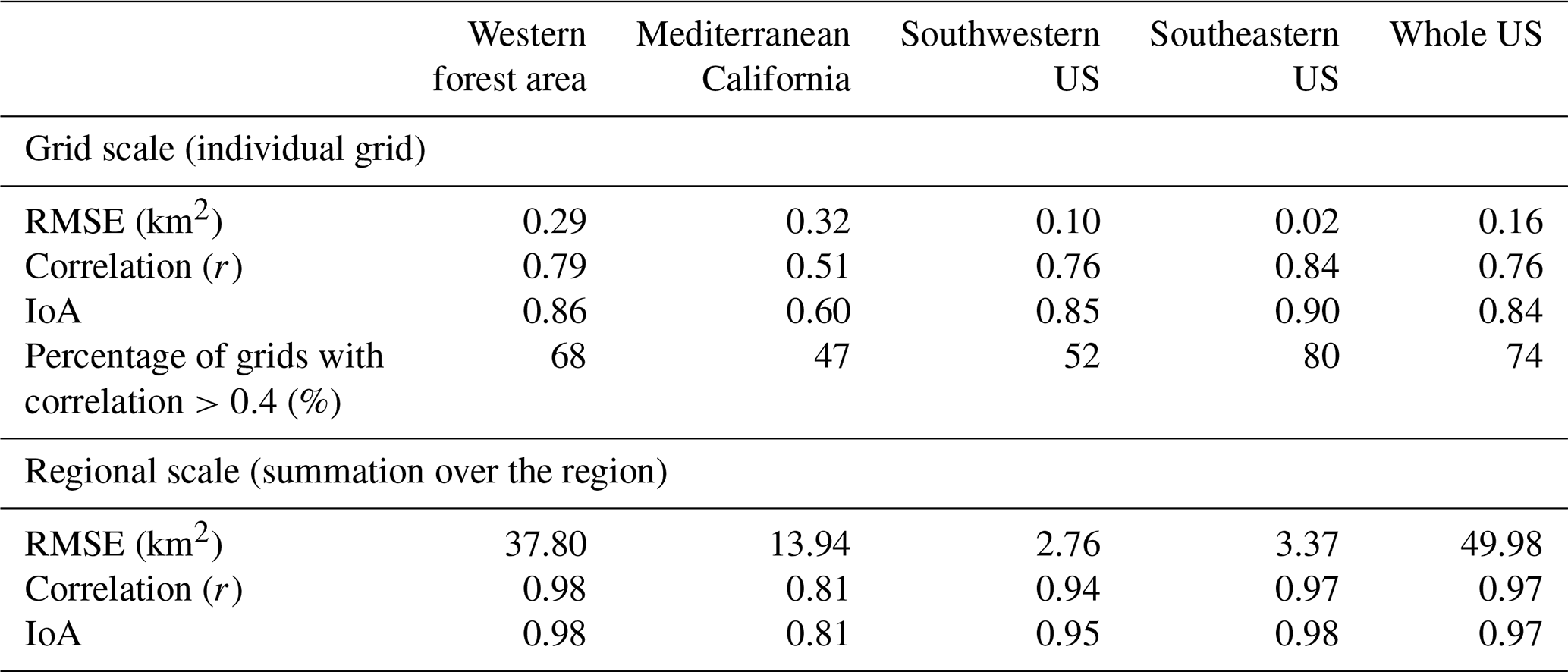
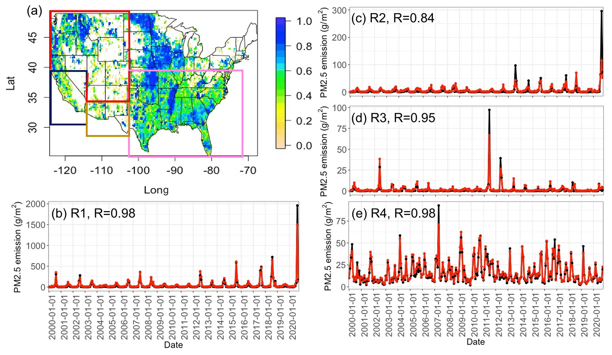
Figure 1(a) The map of temporal correlation between observed and predicted fire PM2.5 emission for each grid. Time series of observed (black) and predicted (red) fire PM2.5 emission average across (b) western forest area (red box in panel a), (c) Mediterranean California (blue box), (d) the southwestern US (dusty box), and (e) the southeastern US (pink box).
To improve understanding of the ML prediction, we utilize the SHAP method to quantify the contributions of each predictor variable to the prediction and identify the key contributing factors of fire PM2.5 emission. SHAP importance is chosen because it provides not only global importance but also local importance that helps understand which variables have larger contributions to specific events or regions. Here, we first demonstrate the global importance that considers all the samples. Figure 2 shows the 20 most important variables for the model ranked by the absolute mean SHAP values. The SHAP value for a feature indicates its contribution to the prediction, so larger absolute mean SHAP values indicate larger contributions to the fire emissions. Among the top 10 variables, seven of them are local meteorological variables, indicating local meteorology is the predominant control of fire emissions, as these variables control fire activity directly (Liu and Wimberly, 2015; Abatzoglou et al., 2016; Wang et al., 2021a). Besides local meteorology, the predictors of large-scale meteorology (SVD1_SElag2 and SVD2_SElag2) are identified as the 8th and 10th important variables, showing that meteorology is important not only at the local scale but also at the synoptic scale (Trouet et al., 2009; Pollina et al., 2013; Dong et al., 2021). Finally, in addition to meteorology, fuel load is identified as the fifth important variable in the model, as fuel load affects emission through controlling burned area and fuel consumption (Seiler and Crutzen, 1980). Considering the important variables in different regions, the selected regions in the western US (western forest area, Mediterranean California, and the southwestern US) generally share the common top 10 variables (Fig. S6). Over the western US, predictors controlling fuel dryness and fuel amount, including RH, fuel moisture (FM1000), ERC, vegetation fraction, and fuel load, contribute more to fire emissions. On the other hand, large-scale meteorological patterns (SVDs_SElag2) are more important for fire emissions in the southeastern US.
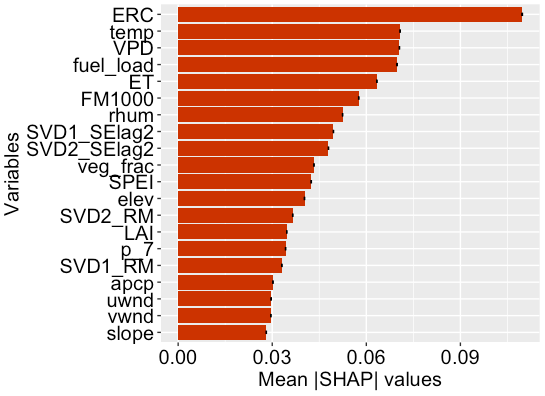
Figure 2Top 20 variables for the model based on the mean absolute SHAP value with the 95 % confidence intervals.
As the dominant drivers differ for different temporal scales, we aggregate the monthly SHAP values to obtain annual and seasonal time series of SHAP values for each variable. The annual and seasonal time series are the averaged SHAP values over the study period for each year and month, respectively. Figure S7 shows the mean |SHAP| values at seasonal and interannual timescales for the CONUS. Considering both the mean |SHAP| and larger correlations (r>0.5) between the annual and seasonal time series of SHAP and mean fire emissions, temperature, VPD, RH, and ERC are the dominant variables controlling the seasonal variation in fire emissions. These factors have relatively stronger seasonality than other variables (e.g., VPD is usually higher in the summer). On the other hand, large-scale circulation patterns, including SVD1_SElag2, SVD2_SElag2, and SVD1_RM, are important variables controlling both the seasonal and interannual variability of fire emissions, while SVD2_RM and SVD2_NCA mainly control interannual variability. Some identified large-scale meteorology has significant seasonality (e.g., SVD1_SElag2 and SVD2_SElag2 are predominant in spring and SVD1_RM is strongest in summer), and most of them have interannual variability, as shown in Fig. 8. Overall, the SHAP analysis shows different dominant predictors for fire emissions at various timescales.
4.2 General comparison between GFED, ML, and FireMIP models
This section compares the performance of the ML and FireMIP models benchmarked against observations from GFED, and the evaluations are based on spatial distributions, seasonality, and interannual variability of fire PM2.5 emissions. Since the spatial resolutions of the GFED data, ML models, and FireMIP models are different, they are all regridded to using bilinear interpolation. Note that the simulation period of FireMIP models ends in 2012, so we use the overlapping period of 2000–2012 for comparison and exclude the MC2 model because its simulation ends in 2008.
4.2.1 Spatial distributions of fire PM2.5 emissions and sensitivities to RH and temperature
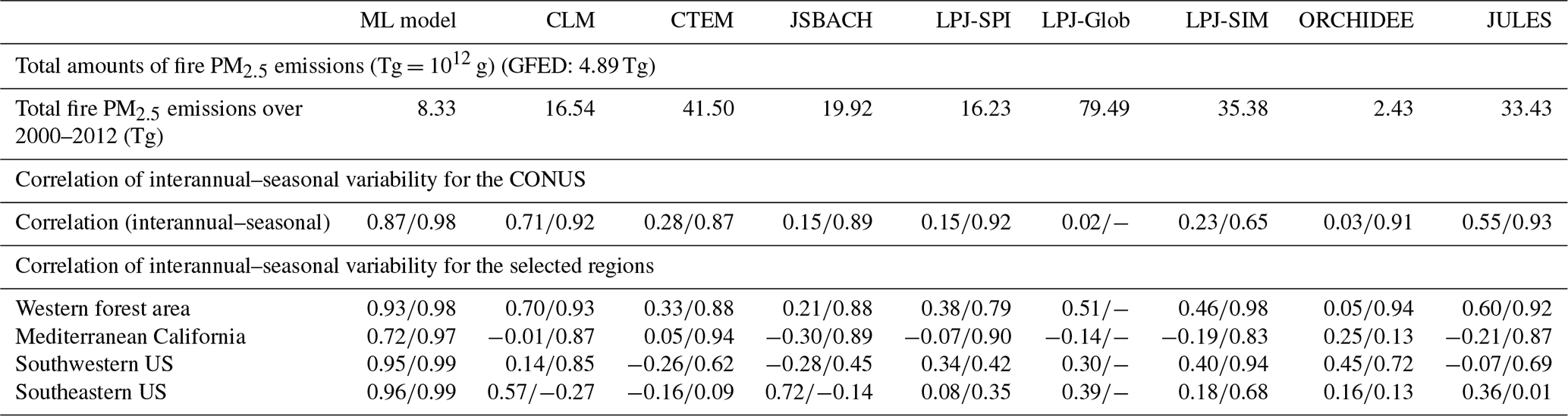
Figure 3 compares the observed and simulated spatial distributions of long-term mean monthly fire PM2.5 emissions averaged over 2000–2012. Among the models, the ML model, CLM, and JULES have better performance in reproducing the spatial distributions of fire emissions over the CONUS, with a correlation coefficient of 0.83, 0.52, and 0.40, respectively. The ML model shows the best agreement with GFED, though it overestimates fire emissions over northern California. Both CLM and JULES simulate more PM2.5 emissions over the southeastern US, and JULES overestimates fire emissions in northern California. Some other models, such as CTEM, JSBACH, and LPJ-SIP, tend to overestimate fire emissions over the central US (e.g., Great Plains and Texas). LPJ-SIM captures the hotspots of fire emissions over the western US and southeastern US, but it simulates much more PM2.5 emissions over the Rocky Mountains and northeastern US. In terms of the total amount of PM2.5 emissions, all models except ORCHIDEE-SPITFIRE overestimate PM2.5 emissions (8.33–79.49 Tg), compared to the GFED estimate of 4.98 Tg during 2000–2012 over the CONUS (Table 4).
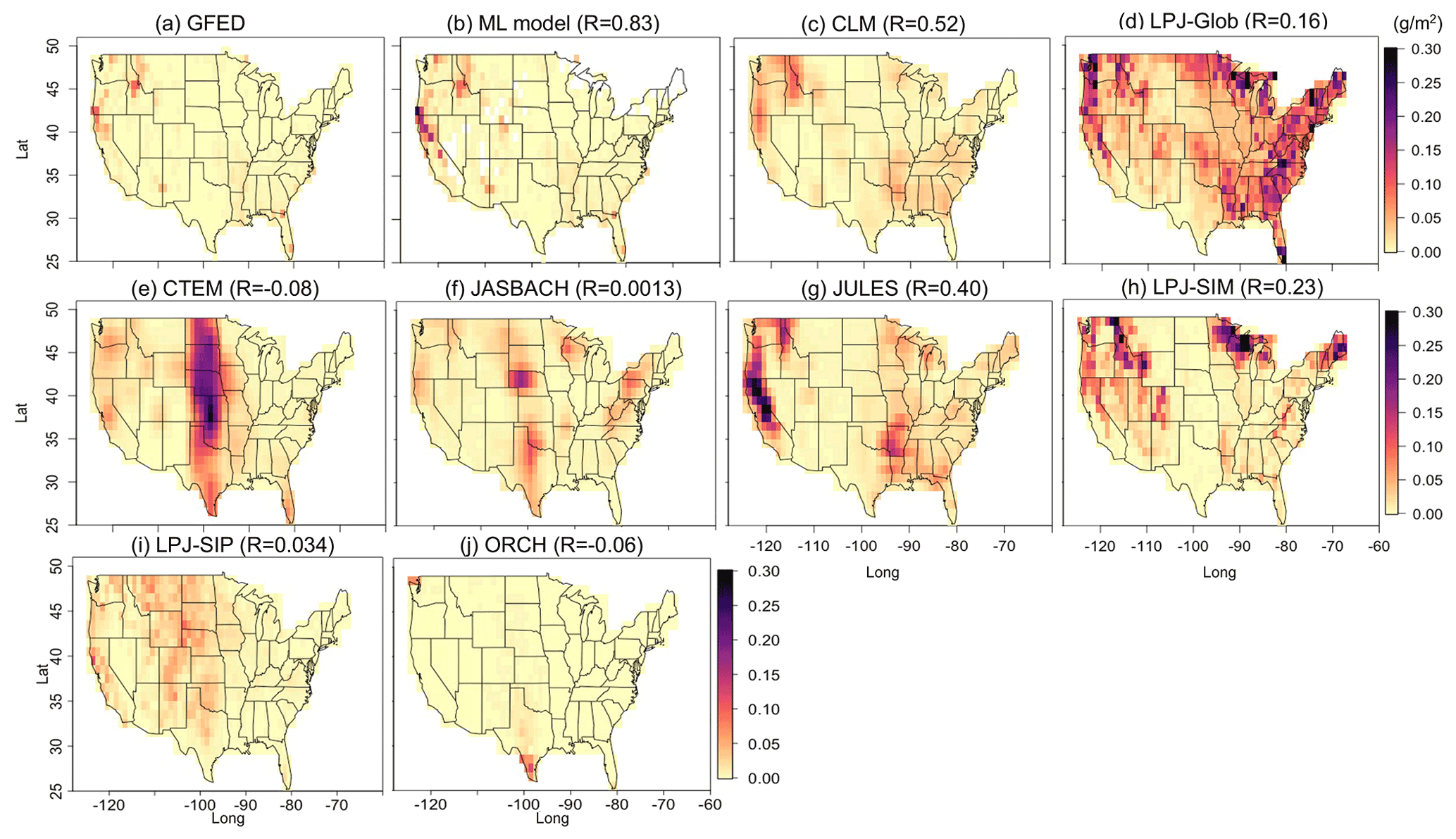
Figure 3Spatial distributions of the monthly mean fire PM2.5 emission (g m−2 per month) over 2000–2012.
Table 4The model performance for the ML model and FireMIP models.
The overestimations in some models may be explained by the sensitivities of fire emissions to individual meteorological variables. Figure 4 shows the slopes for the dependence of annual mean fire PM2.5 emissions on annual mean RH from the CRUNCEP atmospheric forcing data for GFED and the 10 models based on linear regression. Since the ML model uses NARR meteorology as predictors, we also include sensitivities of the fire emissions predicted by the ML model to the NARR meteorology (Fig. 4b). Almost all models capture the negative dependence of PM2.5 emissions on RH over the western US (), but the sensitivities in the models are much stronger (steeper negative slope) than in GFED. For temperature, positive sensitivity is shown over the western US in GFED (Fig. 5), with the largest slope in northern California. The sensitivities to temperature in models agree with the observed sensitivities (), but some models show much stronger sensitivities over the western, central, and southeastern US. Generally, the spatial distributions of the long-term mean fire emissions shown in Fig. 3 match well with the spatial distributions of sensitivities to RH or temperature, suggesting an important role of the sensitivities in the model biases of predicting fire emissions. However, the correspondence of large fire emissions to the sensitivities to RH or temperature shows regional differences. For instance, in the western US, the stronger sensitivities to both RH and temperature correspond to the overestimations in this region for most models, including the ML model, CLM, CTEM, JSBACH, JULES, LPJ-SIM, and LPJ-SPI (Figs. 4 and 5). On the other hand, over the central US, larger PM2.5 emissions simulated by CTEM and JSBACH only correspond to stronger sensitivity to temperature (Fig. 5). Similar to the central US, in the southeastern US, the overestimations in CLM and JULES only correlate with stronger sensitivity to temperature (Fig. 5). Regional differences in the correspondences between the predicted fire emissions and their sensitivity to meteorology can be explained by several factors. For the western US, the overestimations of fire emissions correspond to stronger sensitivities to both RH and temperature, given that fire activities are sensitive to fuel aridity that is controlled by temperature and fuel moisture (Abatzoglou and Williams, 2016; Holden et al., 2018). As for the southeastern US, fuels in this region typically burn at higher RH, and the interannual RH variation (standard deviation) is smaller (Balch et al., 2017; Brey et al., 2018). With higher RH values and less variation in RH, the fire emissions in the southeastern US show weaker sensitivity to RH than to temperature in observation (Table S2). The above analysis shows that the overestimation of fire emissions in the models may be attributed to the stronger sensitivities to meteorology. However, fire activities are controlled by meteorology and other factors such as vegetation and humans, so the analysis of fire emission sensitivity to meteorology only provides a potential explanation of the overestimation of fire emissions in the models (Forkel et al., 2019).
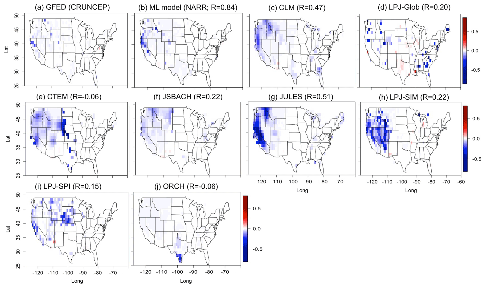
Figure 4Spatial distributions of the linear regression slope for the dependence of annual mean fire PM2.5 emissions on annual mean RH. Only the grids with slopes that are statistically significant (p<0.05) are shown.
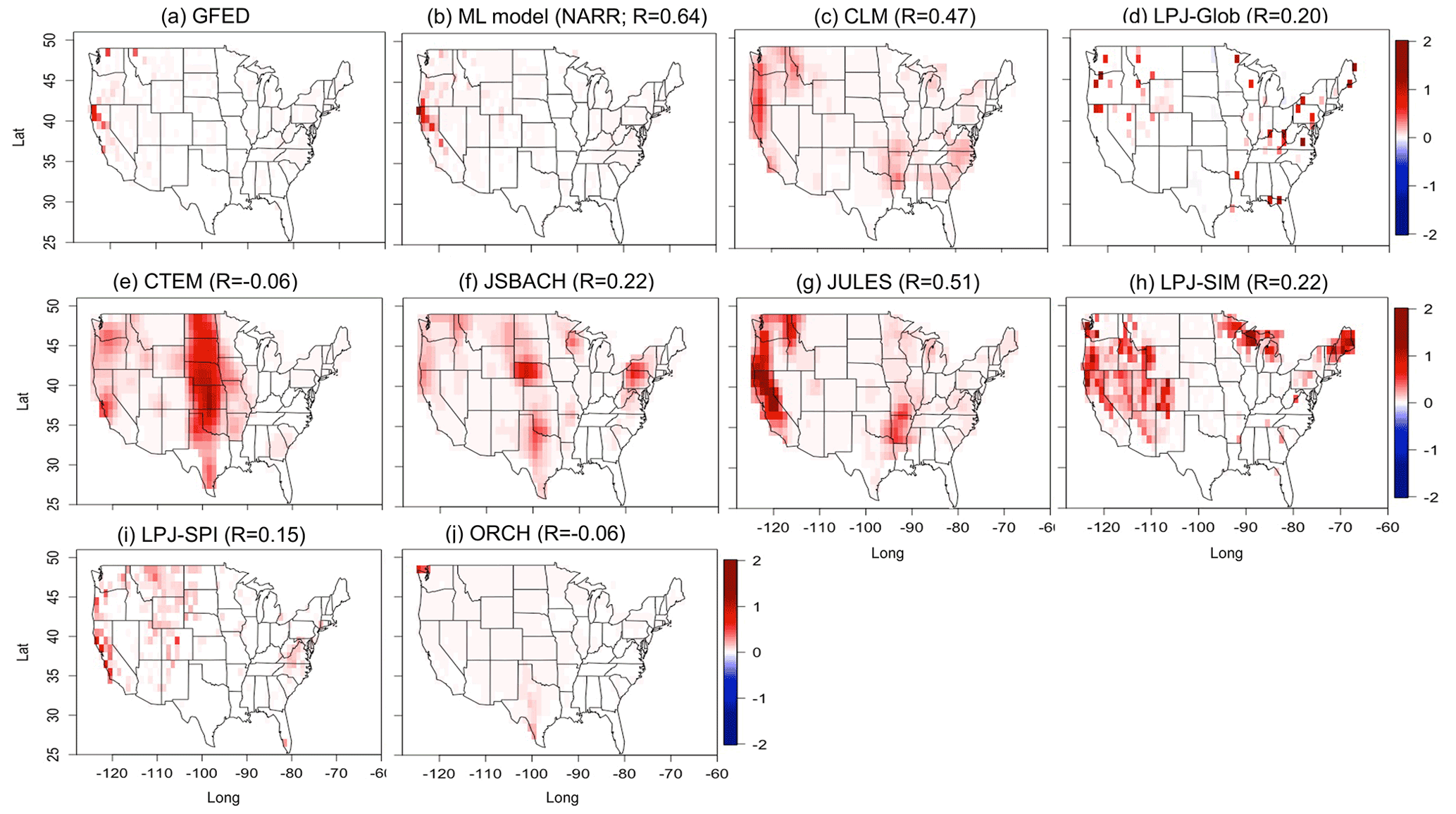
Figure 5Spatial distributions of the linear regression slope for the dependence of annual mean fire PM2.5 emissions on annual mean temperature. Only the grids with slopes that are statistically significant (p<0.05) are shown.
4.2.2 Seasonality and interannual variability over the CONUS
In addition to evaluating spatial distributions, it is also important to compare the models' ability to reproduce the temporal variability of fire emissions. As the models may systematically over- or underestimate fire emissions, we normalize the emissions by the mean and standard deviation and focus only on its temporal variability. Figure 6a shows the seasonality of normalized fire PM2.5 emission over the CONUS. Most models capture the seasonality of fire emission successfully (r>0.85), except LPJ-SIM, which simulates peak emission in August–October (r=0.65). Among the models, the ML model has the highest correlation coefficient between prediction and observation from GFED (r=0.98) and successfully reproduces the peak in August. The seasonal peaks simulated by the FireMIP models are broader and flatter than the peak in GFED, with an early peak in June–July continuing to September (Fig. 6a).
In terms of interannual variability (Fig. 6b), the ML model, CLM, and JULES perform better than other models, with larger correlation coefficient between simulated and observed fire PM2.5 emissions (r=0.87, 0.71, and 0.55 for ML, CLM, and JULES, respectively; Table 4). Other models have relatively poor performance in capturing the interannual variability. The interannual variability of fire emissions shows several peaks in 2002, 2007, and 2012 (black line in Fig. 6b), when the western US contributes 76 % of the total emissions to the peaks in these years. Almost all models except ORCHIDEE capture the peak in 2012. However, most models miss the peaks in 2002 and 2007. Among all models, the LPJ-Glob model simulates the peaks in the two years, while ML, JULES, and CLM only capture the largest emission in 2007 (Fig. 6b).
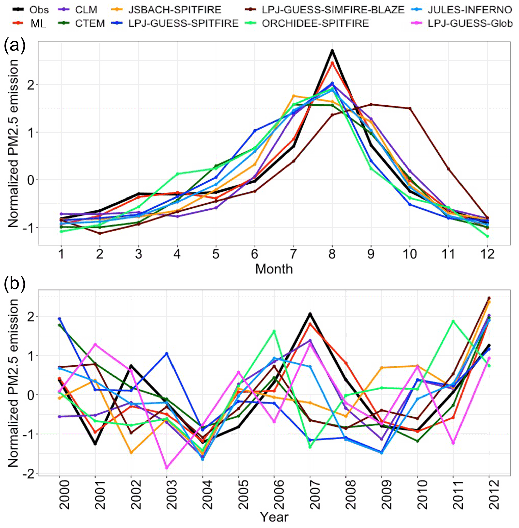
Figure 6(a) Seasonality and (b) interannual variability of the normalized averaged fire PM2.5 emission from the GFED (black line), ML model (red line), and FireMIP models (color lines). The fire PM2.5 emissions are first averaged over the CONUS and normalized by the monthly (annual) mean and standard deviation for seasonality (interannual variability) plots.
4.2.3 Seasonality and interannual variability by regions
As the temporal variability of fire activities varies by region, we compare the performance between GFED and the ML and FireMIP models by the regions defined in Sec. 4.1. Figure 7 shows the seasonality and interannual variability of normalized fire PM2.5 emission over western forest area, Mediterranean California, the southwestern US, and the southeastern US. All models generally capture the seasonality of the western forest area peaking in summer, with correlation coefficients larger than 0.8 (Table 4). Even though the FireMIP models generally reproduce the peaks in summer, the predicted peaks are broad and flat, indicating a relatively longer fire season starting in June and ending in September (Fig. 7a). When looking at the interannual variability, we find that the ML model has the best performance with a correlation coefficient of 0.93, and it successfully captures the largest fire emission in 2007. CLM, JULES, and LGJ-Glob perform better than the rest of the models (r=0.70, 0.60, and 0.51 for CLM, JULES, and LPJ-Glob, respectively; Table 4), but all of them still miss the peaks in 2007 and overestimate fire emissions in 2001 and 2003 (Fig. 7b). The emission peak in 2007 is mainly attributed to the large fires in Idaho, which were associated with synoptic weather patterns characterized by positive geopotential height and temperature anomalies over the Pacific Coast and western US (Zhong et al., 2020). Consistent with prior findings, SHAP importance shows that in the ML model SVD predictors (SVD_NCA and SVD_RM in July and August 2007, Fig. 8a) are the dominant factors of fire emissions in 2007 (contribute 27 % and 28 % for July and August 2007, respectively), which are characterized by high pressure, low RH, and northeasterly winds over the western US (Figs. S1 and S2). Thus, the underestimation of peak emission in 2007 may be explained by the fact that the influences of large-scale meteorology on fire activity are not fully considered in the FireMIP models, which are point models driven only by local atmospheric forcing.
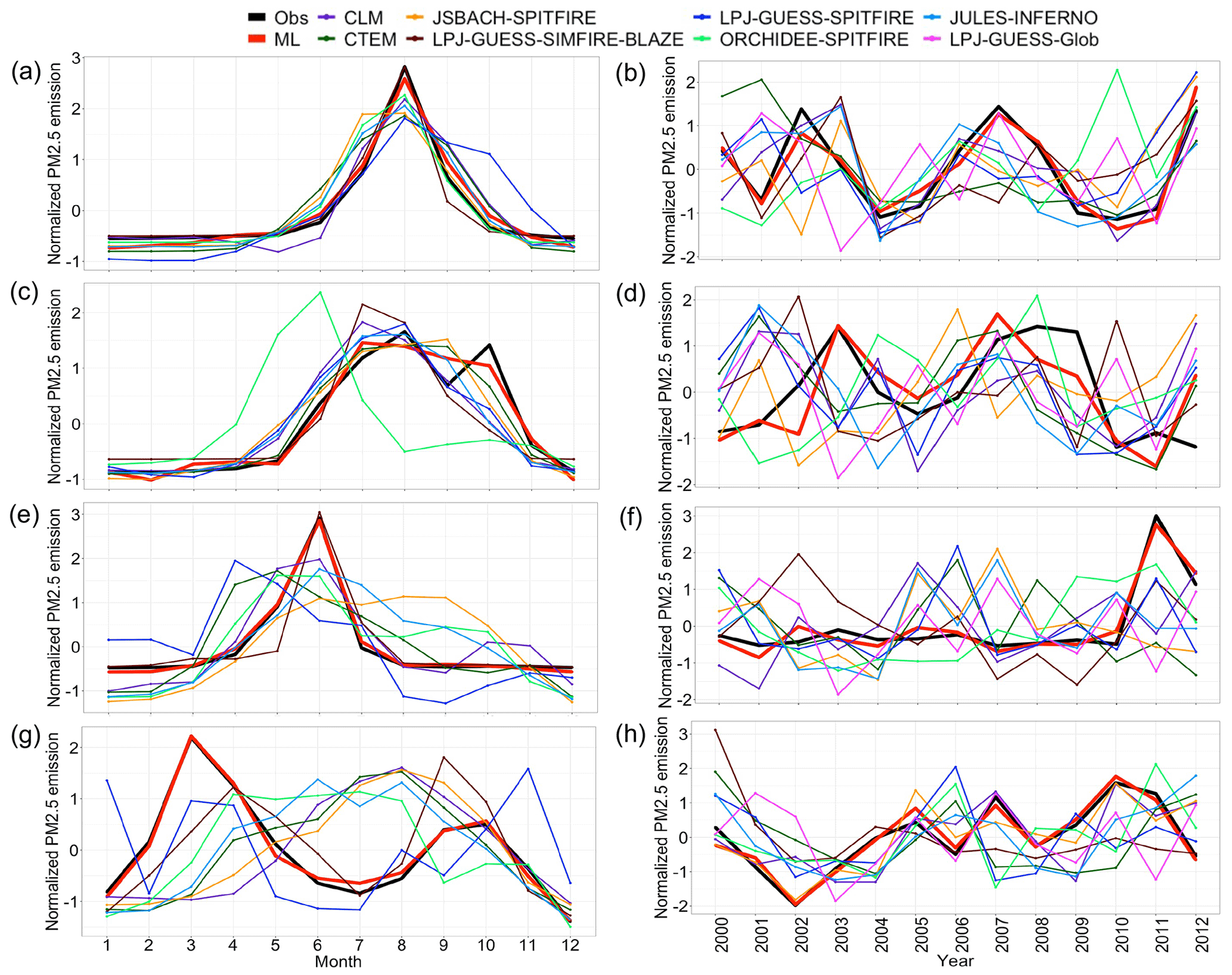
Figure 7Seasonality and interannual variability of the fire PM2.5 emission from the GFED (black line), ML model (red line), and FireMIP models (color lines) for (a, b) western forest area, (c, d) Mediterranean California, (e, f) the southwestern US, and (g, h) the southeastern US.
In Mediterranean California, the seasonality of fire emissions shows a bimodal pattern, peaking in August and October. The peak in October is mainly due to the extremely large fires associated with Santa Ana winds in 2003 and 2007 (Keeley et al., 2009; Yue et al., 2014). The ML model simulates a flatter peak from July to October, while all the FireMIP models except ORCHIDEE capture the first emission peak in summer but fail to simulate the large fire emission in October (Fig. 7c). The underestimation associated with the Santa Ana winds is also shown in the interannual time series in Fig. 7d. Several models, including LPJ-Glob, CTEM, LPJ-SPI, and JULES, capture the peak in 2007, but only the ML model predicts both peaks in 2003 and 2007 even though the peak in 2003 is underestimated. According to the SHAP importance from the ML model, the peak emissions in October 2003 and October 2007 are mainly contributed by the SVD predictors and ERC (SVD2_NCA and SVD1_RM together contribute 20 % to the fire emissions for October 2003 and SVDs_SElag2 and SVD2_RM together contribute 31 % to the fire emissions for October 2007) and ERC (15 % and 18 % for October 2003 and 2007, respectively) (Fig. 8b). The results indicate that the ML model captures the effect of synoptic weather patterns on fire activity by including the SVD predictors. Even though the wind speed is included in simulating fire spread in the FireMIP models, the spatial resolutions of the models and/or the atmospheric forcing data may not be fine enough to resolve the strengthened offshore winds through the complex terrain, and subsequently, they may not capture the effects of Santa Ana winds on fires well. As shown in Fig. S8, the wind speeds from NARR are significantly larger than from CRUNCEP for the strong wind days (daily wind speed >4.5 m s−1) over southwestern California (32.6–34.8∘ N, 116–119∘ W) during October 2000–2012 as well as during October 2003 and 2007 (Table S3). The results indicate the lower wind speeds in the CRUNCEP atmospheric forcing used in FireMIP may partially explain the model biases for the events associated with Santa Ana winds. Besides the abovementioned shortfall, all the models have problems reproducing the interannual variability of the fire emissions over Mediterranean California, with very low correlations (r<0.25) for the FireMIP models and a relatively low correlation (r=0.72) for the ML model (Table 4; Fig. 7d). The poor performance for this region may be due to the complex relations between fires and multiple factors, including meteorology, complex terrain, fuel, and human, which may not be fully represented in the models (Mann et al., 2016; Radeloff et al., 2018).
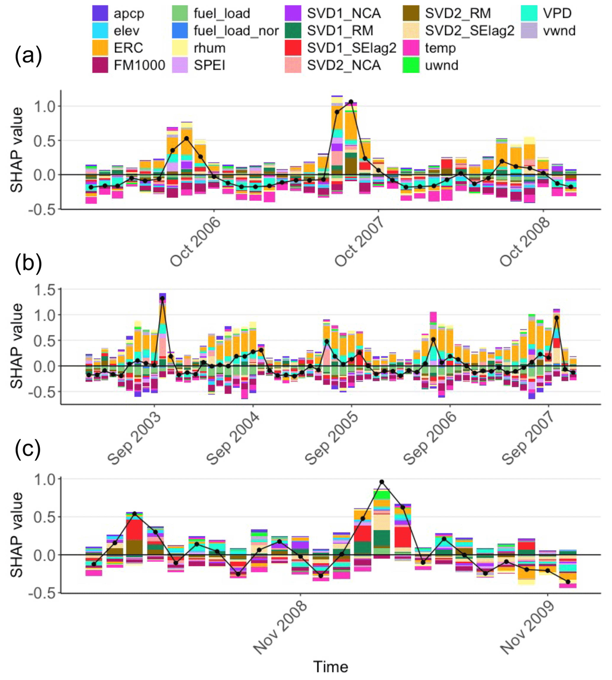
Figure 8Time series of the average SHAP values (bar) and predicted normalized fire PM2.5 emission (line) for (a) western forest area from 2006 to 2008, (b) Mediterranean California from 2003 to 2007, and (c) the southeastern US from 2008 to 2009. The SHAP values indicate the contribution of the predictors to the prediction of normalized fire emission.
Both the ML model and LPJ-SIM successfully reproduce the seasonality of fire emission in the southwestern US peaking in June (r=0.99 and 0.94 for ML and LPJ-SIM, respectively), while other models simulate relatively smooth seasonality (Fig. 7e and Table 4). The ML model, LPJ-SIM, and ORCHIDEE have better performance for the interannual variability, with correlation coefficients of 0.95, 0.40, and 0.45, respectively (Table 4). However, most FireMIP models show larger variability in fire emissions than the GFED, and they all fail to capture the extremely large fire emission in 2011 (Fig. 7f). The peak fire emission in 2011 over the southwestern US was caused by extremely low atmospheric moisture along with moderately high temperature, leading to record-breaking VPD and wildfire activities (Williams et al., 2015). To explain why the FireMIP models fail to capture the peak of 2011, we compare the VPD calculated from CRUNCEP data and the VPD data from gridMET used in the ML model. As Fig. S9 shows, CRUNCEP shows smaller positive anomalies of VPD over the southwestern US in summer 2011, while gridMET data demonstrate a significantly larger VPD anomaly. The biases in CRUNCEP data may partially explain the underestimations in all FireMIP models.
For the southeastern US, the seasonal cycle of fire PM2.5 emissions displays a bimodal pattern, peaking in spring (March–April) and fall (September and October) (Fig. 7g). Most models fail to reproduce the bimodal fire emissions, but the ML model, LPJ-SIM, and LPJ-SPI can capture the bimodal pattern. Although LPJ-SIM and LPJ-SPI predict the bimodal peaks, the first peak simulated by LPJ-SIM shows a 1-month delay, and the second peak simulated by LPJ-SIM and LPJ-SPI is 1 month early and 1 month late, respectively (Fig. 7g). In addition, the ML model, CLM, and JSBACH reproduce the interannual variability of fire PM2.5 emissions relatively well (r=0.96, 0.57, and 0.72 for the ML model, CLM, and JSBACH, respectively) (Table 4 and Fig. 7h). Interestingly, CLM and JSBACH can capture several peaks in 2007, 2010, and 2011, but they do not simulate seasonality correctly, which may be explained by the fact that the underestimation in spring is compensated for by the overestimation in summer related to abnormal dryness or drought.
4.3 Performance in modeling extreme events
Fire activity in the US is becoming more hazardous, particularly over the western US, due to more frequent hotter and drier conditions as climate continues to warm (Williams et al., 2019). Thus, it is necessary to assess whether the ML model and process-based models can capture the extreme events in terms of their magnitude, frequency, timing, and location, which is essential to future projection and adaptation. As CLM performs relatively well among the FireMIP models, we select CLM for comparison with the ML model at resolution, focusing on the spatial patterns of extreme event frequency and two case studies with extremely large fire emissions.
4.3.1 Frequency of extreme event occurrence
Figure 9 shows the frequency maps of months with large fire emissions during 2000–2012 for GFED, the ML model, and CLM. Large fire emission is defined as monthly fire PM2.5 emissions greater than the 95th percentile of fire PM2.5 emission considering all the grids over the CONUS in 2000–2012. GFED shows hotspots with a higher frequency over northern California, the Pacific Northwest, and the southeastern US, with total counts ranging from 15 to 105 (Fig. 9a). The ML model captures the spatial patterns (r=0.74), but it overestimates the number of months by a factor of 2 to 3 compared to GFED, especially over the western US (Fig. 9b). The spatial patterns of large fire emission occurrence simulated by CLM are generally consistent with the observed distribution by GFED (r=0.35). However, it overestimates the frequency, particularly over Idaho and the northeastern US, and simulates more significant numbers of months with extreme events over large spatial extents, maybe due to its coarse spatial resolution (Fig. 9c).
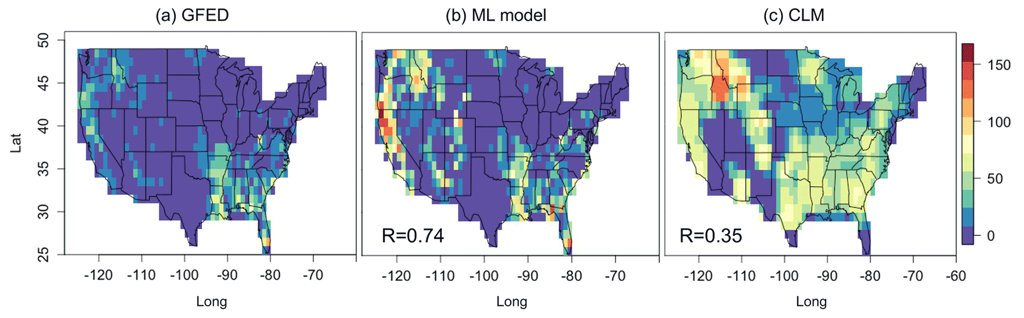
Figure 9Spatial distributions of number of months with large fire emissions (> 95th percentiles of fire PM2.5 emission over all the grids in 2000–2012) for (a) GFED, (b) the ML model, and (c) CLM.
4.3.2 Case studies
To evaluate how well the models simulate the large fire emissions, we compare model performance for the two recent cases reported to be the largest fire events during 2000–2012, including the fires in the southern US in 2011 and western US in 2012. During 2011, a severe drought leading to large wildfires was observed over the southern US, including Arizona, New Mexico, and Texas (NOAA, 2012; Wang et al., 2015). Figure 10 shows the maps of annual mean fire PM2.5 emissions over the southern US from GFED, the ML model, and CLM. GFED shows the largest fire emissions close to the border of Arizona and New Mexico in conjunction with other small hotspots over New Mexico, Texas, and Louisiana (Fig. 10a). The ML model overall reproduces the spatial distributions of the fire emissions (r=0.96) and captures the largest fire emission in Arizona and New Mexico in 2011 (Fig. 10b). However, CLM does not capture the hotspots observed in GFED over Arizona and New Mexico but simulates larger fire emissions in Louisiana instead (Fig. 10c). In terms of the time series, the ML model reproduces the temporal variability of fire emissions and successfully captures the peak of total fire PM2.5 emissions in June 2011 (r=0.98; Fig. 10d and e). Although CLM simulates the peak in June, it overestimates fire emissions in the following months by a factor of 4 (r=0.52; Fig. 10d and e).

Figure 10Top panel: spatial distributions of the annual mean fire PM2.5 emission in 2011 for (a) GFED, (b) the ML model, and (c) CLM. Bottom panel: time series of the (d) total fire PM2.5 emissions and (e) normalized fire PM2.5 emission over the southern US domain during 2011.
In 2012, the western US experienced several major wildfires (NOAA, 2013). The warm and dry conditions led to large wildfires in California, Oregon, New Mexico, and Colorado (Fig. 11). Both the ML model and CLM capture the hotspots with large fire emissions (Fig. 11b and c) and have correlation coefficients of 0.56 and 0.37, respectively. However, the ML model tends to overestimate fire emissions, especially in areas surrounding the grids with extremely large fire emissions (Fig. 11b). CLM misses some large fire emissions in Colorado and New Mexico and underestimates the larger fire emissions in several hotspots (Fig. 11a), which may be explained by its coarse resolution. The time series of normalized fire PM2.5 emissions in 2012 show one peak in August. The ML model captures the peak and presents a high correlation between the simulated and observed normalized and total fire PM2.5 emissions (r=0.98). CLM captures the peak in August but overestimates emissions in September and October (r=0.84; Fig. 11d and e). To test model generalization, we train the model using data of 2000–2009 and 2013–2020 and test on 2010–2012 and compare the ML performance with CLM (Figs. S10–S11). The ML model performance is as good as the 10-fold cross-validation, demonstrating that the ML model performs well on predicting unseen data.

Figure 11Top panel: spatial distributions of the annual mean fire PM2.5 emission in 2012 for (a) GFED, (b) ML model, and (c) CLM. Bottom panel: time series of the (d) total fire PM2.5 emissions and (e) normalized fire PM2.5 emission over the western US domain during 2012.
This study provides the first assessment to evaluate the performance of data-driven and process-based models in predicting fire PM2.5 emissions over the CONUS. We first demonstrate that the developed ML model performs well in predicting monthly fire PM2.5 emissions nationwide at grid cells of resolution from 2000 to 2020, with an RMSE of 0.16 g m−2 and IoA of 0.84. The ML model outperforms prior statistical models predicting fire activities at similar spatial and temporal scales (Carvalho et al., 2008; Bedia et al., 2014). Considering the performance at a regional scale, the ML model reproduces the interannual variability of fire emissions for the selected regions, with correlation coefficients ranging from 0.84 to 0.98. Therefore, the ML model has a promising performance in predicting fire emission over the CONUS at a relatively fine spatial resolution. Compared to the wildfire-burned-area model in Wang et al. (2021a), the fire emission model in this study shows slight degradations in capturing the interannual variability of fire emission at grid level (e.g., percentage of grids with correlations larger than 0.4). This may be explained by the fact that the fire emission model may not effectively resolve the relationships between fires and predictors when more grids with less fire occurrence are included (i.e., more zeros or unburned grids) without reliable information about ignition. As a side note, both burned area and emission ML models have relatively poor performance over Mediterranean California, indicating the challenges in modeling fire activities in this region where the terrain and land use are complex. The SHAP variable importance shows that meteorology at both local and synoptic scales as well as fuel loads are important variables controlling fire emissions over the CONUS. Regional analysis of predictors indicates that fuel dryness such as fuel moisture and energy release component (ERC) and fuel load are important for predicting fire emissions in the western US, while large-scale meteorological patterns (SVDs_SElag2) contribute more to fire emissions in southeastern US.
We then compare the simulated fire PM2.5 emissions from the ML model and FireMIP models against GFED from 2000 to 2012 at the spatial resolution of . The ML model, CLM, and JULES reproduce the spatial distribution more reasonably than the rest of the FireMIP models (r=0.83, 0.52, and 0.40 for the ML, CLM, and JULES, respectively). Both CLM and JULES simulate more fire PM2.5 emissions over the southeastern US, which can be explained by several reasons. First, it has been shown that the satellite-observed burned areas in the southeastern US are much smaller than the burned areas estimated from the ground-based fire records, which might have resulted from the small prescribed and agricultural fires (Hu et al., 2016; Nowell et al., 2018). In addition, large differences exist among different satellite-estimated fire PM2.5 emissions in the southeastern US (Li et al., 2019a). As a consequence, these studies highlighted uncertainties about the GFED-estimated burned area and emission over the southeastern US. Second, cropland fires are one of the predominant fire types in this region. Among the FireMIP models, CLM is the only model that simulates cropland fires (Li et al., 2013). For JULES, even though it does not simulate cropland fires, it treats croplands as natural grasslands. The emission factors of grasslands and croplands used in the FireMIP models are larger than in GFED4s, thereby causing larger fire PM2.5 emissions in the southeastern US in CLM and JULES (van der Werf et al., 2017; Li et al., 2019a). Furthermore, Li et al. (2019a) noted that CLM4.5 simulates higher fuel loads in croplands than the CASA model used by GFED4s, leading to higher fire carbon emissions estimated by CLM than by GFED. It is worth noting that the ML model incorporates fuel load simulated by CLM4.5, but it predicts fire emissions closer to GFED4s, indicating a smaller sensitivity of fire emission to fuel load in the ML model. Lastly, the overestimation of fire PM2.5 emissions can also be explained by the sensitivity to meteorology. The spatial distributions of the long-term mean fire emissions shown in Fig. 3 correlate with the spatial distributions of sensitivities to RH and/or temperature, with regional differences. For the western US, large fire emissions are associated with stronger sensitivities to both RH and temperature in the ML and most FireMIP models. For the central and southeastern US, overestimation of fire PM2.5 emissions only corresponds to stronger sensitivity to temperature in some FireMIP models.
Besides comparing model performance aggregated over the CONUS, we analyze the model performance for several regions, including the western forest area, Mediterranean California, the southwestern US, and the southeastern US. For the western forest area, the ML model performs well in capturing both seasonality and interannual variability of fire PM2.5 emissions, with correlation coefficients of 0.98 and 0.96, respectively. In contrast, the FireMIP models generally reproduce the seasonality well but do not simulate the interannual variability well, especially underestimating the peak in 2007, which related to large-scale meteorological patterns favorable for fires in the Pacific Northwest (Zhong et al., 2020). For Mediterranean California, all FireMIP models only capture the first peak in August but fail to simulate the second peak in October, which is caused by large fires related to Santa Ana winds in 2003 and 2007. Such lack of peak emission is also shown in the interannual variability, as all FireMIP models show limited ability to simulate the peaks in these two years. By contrast, the ML model successfully predicts the bimodal seasonality and the large fire emissions related to the Santa Ana winds in 2003 and 2007. The underestimation of the peak in the FireMIP models may be attributed to the underrepresentation of the effects of large-scale meteorology in the two regions, as the ML model and SHAP importance show that SVD predictors have larger contributions to the fire emissions in both events. The results of the two regions in the western US suggest that fire parameterization in the FireMIP models could be improved by including the effects of regional and large-scale meteorology (e.g., Santa Ana winds) on fire activity (Yue et al., 2014). Modeling the effect of Santa Ana winds on wildfires may be particularly challenging as the offshore Santa Ana winds exhibit variability related to both synoptic-scale pressure anomaly over the Great Basin and local thermodynamic forcing associated with strong desert–ocean temperature gradient (Hughes and Hall, 2010).
As for the southwestern US, the ML model and LPJ-SIM estimate the peak in June (r=0.99 and 0.94 for ML and LPJ-SIM, respectively), which highly agrees with the GFED observation. Interestingly, most FireMIP models fail to capture the extremely large fire emission in the 2011 summer mainly due to the low biases of VPD anomalies in CRUNCEP (Tang et al., 2017). Unlike the southwestern US, the seasonality of the southeastern US has peaks in March–April and September–October. The two peaks of fire emissions correspond to wildfires (March–April and September), cropland fires (February–March and August–October), and prescribed fires (February–April and October) that include burnings for pest controls and land cleaning (Knapp et al., 2009; Lin et al., 2014). Most models fail to reproduce the bimodal fire emissions, but the ML model, LPJ-SIM, and LPJ-SPI can capture the bimodal pattern. Even though the seasonality of fires over this region is not simulated accurately, the CLM and JSBACH reproduce the interannual variability of fire PM2.5 emissions and predict the peaks well. The FireMIP models' shortfall in reproducing the bimodal seasonality can be explained by two reasons. First, the relationships between humans and fire spread implemented in the process-based models may not be realistic compared to the observed relationships. Parisien et al. (2016) demonstrated the large spatial variability of human impacts on burned areas in North America, which is not well represented in the FireMIP models (Li et al., 2019a). Second, drier conditions in winter would promote fires in springtime (Wear and Greis, 2013; Wang et al., 2021a), which may not be directly considered in the FireMIP models but are incorporated as SVD predictors in the ML model. Overall, the representations of the effects of human and large-scale meteorology on fires may explain why the models simulate the seasonality incorrectly in the southeastern US. In addition to the comparison of general model performance, we also compare the ability of the data-driven and processed-based models in predicting extremely large fire emissions. Both ML and CLM models reproduce the spatial pattern of extreme fire events and reasonably simulate the historical events of large fires in the southwestern and western US.
It is known that different fire emission inventories have their uncertainties, and prior studies have compared fire emission inventories over the globe or the CONUS (Urbanski et al., 2018; Liu et al., 2020). The GFED fire emissions used in this study are known to underestimate the fire emission peak in springtime over the southeastern US, which may be explained by the fact that other products such as FINN or QFED capture more small fire activity compared to the GFED approach (Koplitz et al., 2018; Carter et al., 2020). Although FINN can capture more small fires, it underestimates the intensity of large fires for some cases, which has been attributed to the cloud coverage on daily-scale detection (Paton-Walsh et al., 2012). QFED and GFAS, which estimate emissions using fire radiative power (FRP) from satellites, are also more sensitive to small fires than GFED. However, QFED tends to estimate much larger emissions than other products, which can be explained by the fact that the emission coefficients used to obtain emissions are constrained by MODIS AOD and the uncertainties within FRP (Pan et al., 2020). Despite the known discrepancy between GFED and other data products, the GFED data still show bimodal peaks in spring and fall over the southeastern US, while most FireMIP models fail to reproduce the first peak (Fig. 7g). For the western US, GFED and FINN are generally consistent regarding the magnitude and variability of fire emissions (Urbanski et al., 2018). As stated above, different fire emission inventories have uncertainties. Future works are required to include other fire emission datasets for model evaluation.
To summarize, we utilize the ML model with SHAP importance to diagnose the fire emissions simulated by process-based models and attributed model biases to several factors. First, the sensitivities of fire emissions to meteorology in the models are stronger than those observed, leading to overestimations. Second, the large-scale meteorological patterns conducive to fires are not fully considered in the process-based models, which are important contributors of large fire emissions in the western US and southeastern US. Third, the spatial resolutions of models and/or the atmospheric forcing they used may be too coarse to resolve the effects of regional weather phenomena such as Santa Ana winds. Fourth, biases in the atmospheric forcing data may result in biases of fire emission predictions. Last but not least, human activities are a critical component shaping fire regimes, but the human effects on fire activities in the FireMIP models may not reflect the human–fire relationships in the real world. This is also an issue in the ML model as the human-related predictors in the ML model may be too simple to represent the human influences. The underrepresentation of human effects in both types of models may cause additional uncertainties in projecting future fire activities and their impacts on climate. By training the ML model using the GFED emissions, the ML model is able to better explain fire emissions in the US, which makes it a useful tool for diagnosing processes or relationships that may be missing or not well represented in the process-based models to guide future development for improving their performance. Besides its use in diagnosing process-based models, the ML model with SHAP provides a different and novel approach to simulate fire emissions more accurately and identify the important predictor variables. While the ML model generally has higher accuracy than the FireMIP models, the feedbacks between fire emissions and climate are not included, which could potentially affect the reliability of ML-based models in fire emission prediction under future climate change scenarios (Zou et al., 2020). Lastly, due to limited training data, the ML model cannot predict fires in regions with longer fire return intervals, posing additional uncertainties in their use for making future projections.
Model code is available upon request to the first author.
The ML prediction and predictor dataset used in this study are publicly accessible online at https://doi.org/10.5281/zenodo.5076646 (Wang et al., 2021b).
The supplement related to this article is available online at: https://doi.org/10.5194/acp-22-3445-2022-supplement.
SSCW, YZ, YQ, and LRL conceived the research ideas. SSCW wrote the initial draft of the paper and performed analyses and model development. All authors contributed to the interpretation of the results and the preparation of the paper.
At least one of the (co-)authors is a member of the editorial board of Atmospheric Chemistry and Physics. The peer-review process was guided by an independent editor, and the authors also have no other competing interests to declare.
Publisher’s note: Copernicus Publications remains neutral with regard to jurisdictional claims in published maps and institutional affiliations.
The views expressed in this document are solely those of the SEARCH Center and do not necessarily reflect those of the Agency. The EPA does not endorse any products or commercial services mentioned in this publication.
This article is part of the special issue “The role of fire in the Earth system: understanding interactions with the land, atmosphere, and society (ESD/ACP/BG/GMD/NHESS inter-journal SI)”. It is a result of the EGU General Assembly 2020, 3–8 May 2020.
This research was performed at PNNL and funded under assistance agreement no. RD835871 by the U.S. Environmental Protection Agency to Yale University through the SEARCH (Solutions for Energy, AiR, Climate, and Health) Center. It has not been formally reviewed by the EPA. We thank the two anonymous reviewers and Xiaohong Liu for helpful comments on the paper.
This research has been supported by the U.S. Environmental Protection Agency (grant no. RD835871).
This paper was edited by Xiaohong Liu and reviewed by two anonymous referees.
Abatzoglou, J. T. and Kolden, C. A.: Relationships between climate and macroscale area burned in the western United States, Int. J. Wildland Fire, 22, 1003–1020, https://doi.org/10.1071/WF13019, 2013.
Abatzoglou, J. T. and Williams, A. P.: Impact of anthropogenic climate change on wildfire across western US forests, P. Natl. Acad. Sci. USA, 113, 11770–11775, https://doi.org/10.1073/pnas.1607171113, 2016.
Abatzoglou, J. T., Kolden, C. A., Balch, J. K., and Bradley, B. A.: Controls on interannual variability in lightning-caused fire activity in the western US, Environ. Res. Lett., 11, 045005, https://doi.org/10.1088/1748-9326/11/4/045005, 2016.
Akagi, S. K., Yokelson, R. J., Wiedinmyer, C., Alvarado, M. J., Reid, J. S., Karl, T., Crounse, J. D., and Wennberg, P. O.: Emission factors for open and domestic biomass burning for use in atmospheric models, Atmos. Chem. Phys., 11, 4039–4072, https://doi.org/10.5194/acp-11-4039-2011, 2011.
Aldersley, A., Murray, S. J., and Cornell, S. E.: Global and regional analysis of climate and human drivers of wildfire, Sci. Total Environ., 409, 3472–3481, https://doi.org/10.1016/j.scitotenv.2011.05.032, 2011.
Amatulli, G., Domisch, S., Tuanmu, M.-N., Parmentier, B., Ranipeta, A., Malczyk, J., and Jetz, W.: A suite of global, cross-scale topographic variables for environmental and biodiversity modeling, 5, 180040, https://doi.org/10.1038/sdata.2018.40, 2018.
Arrieta, A. B., Díaz-Rodríguez, N., Del Ser, J., Bennetot, A., Tabik, S., Barbado, A., Garcia, S., Gil-Lopez, S., Molina, D., Benjamins, R., Chatila, R., and Herrera, F.: Explainable Artificial Intelligence (XAI): Concepts, taxonomies, opportunities and challenges toward responsible AI, Inform. Fusion, 58, 82–115, https://doi.org/10.1016/j.inffus.2019.12.012, 2020.
Balch, J. K., Bradley, B. A., Abatzoglou, J. T., Nagy, R. C., Fusco, E. J., and Mahood, A. L.: Human-started wildfires expand the fire niche across the United States, P. Natl. Acad. Sci. USA, 114, 2946–2951, https://doi.org/10.1073/pnas.1617394114, 2017.
Bartier, P. M. and Keller, C. P.: Multivariate interpolation to incorporate thematic surface data using inverse distance weighting (IDW), Comput. Geosci., 22, 795–799, https://doi.org/10.1016/0098-3004(96)00021-0, 1996.
Bedia, J., Herrera, S., and Gutiérrez, J. M.: Assessing the predictability of fire occurrence and area burned across phytoclimatic regions in Spain, Nat. Hazards Earth Syst. Sci., 14, 53–66, https://doi.org/10.5194/nhess-14-53-2014, 2014.
Birch, D. S., Morgan, P., Kolden, C. A., Abatzoglou, J. T., Dillon, G. K., Hudak, A. T., and Smith, A. M. S.: Vegetation, topography and daily weather influenced burn severity in central Idaho and western Montana forests, Ecosphere, 6, 1–23, https://doi.org/10.1890/ES14-00213.1, 2015.
Brey, S. J., Barnes, E. A., Pierce, J. R., Wiedinmyer, C., and Fischer, E. V.: Environmental Conditions, Ignition Type, and Air Quality Impacts of Wildfires in the Southeastern and Western United States, Earth's Future, 6, 1442–1456, https://doi.org/10.1029/2018EF000972, 2018.
Carter, T. S., Heald, C. L., Jimenez, J. L., Campuzano-Jost, P., Kondo, Y., Moteki, N., Schwarz, J. P., Wiedinmyer, C., Darmenov, A. S., da Silva, A. M., and Kaiser, J. W.: How emissions uncertainty influences the distribution and radiative impacts of smoke from fires in North America, Atmos. Chem. Phys., 20, 2073–2097, https://doi.org/10.5194/acp-20-2073-2020, 2020.
Carvalho, A., Flannigan, M. D., Logan, K., Miranda, A. I., and Borrego, C.: Fire activity in Portugal and its relationship to weather and the Canadian Fire Weather Index System, Int. J. Wildland Fire, 17, 328–338, https://doi.org/10.1071/WF07014, 2008.
Center For International Earth Science Information Network (CIESIN): Gridded Population of the World, Version 4 (GPWv4): Population Density, Revision 11, Columbia University, NASA Socioeconomic Data and Applications Center (SEDAC) [data set], https://doi.org/10.7927/H49C6VHW, 2017.
Chen, T. and Guestrin, C.: XGBoost: A Scalable Tree Boosting System, in: Proceedings of the 22nd ACM SIGKDD International Conference on Knowledge Discovery and Data Mining, 13–17 August 2016, New York, NY, USA, 785–794, https://doi.org/10.1145/2939672.2939785, 2016.
Coffield, S. R., Graff, C. A., Chen, Y., Smyth, P., Foufoula-Georgiou, E., and Randerson, J. T.: Machine learning to predict final fire size at the time of ignition, Int. J. Wildland Fire, 28, 861–873, 2019.
Cortez, P. and Morais, A.: A Data Mining Approach to Predict Forest Fires using Meteorological Data, in: Proceedings of the 13th Portuguese Conference on Artificial Intelligence, 3–7 December 2007, Guimarães, Portugal, 512–523, 2007.
Crevoisier, C., Shevliakova, E., Gloor, M., Wirth, C., and Pacala, S.: Drivers of fire in the boreal forests: Data constrained design of a prognostic model of burned area for use in dynamic global vegetation models, J. Geophys. Res.-Atmos., 112, D24112, https://doi.org/10.1029/2006JD008372, 2007.
Crimmins, M. A.: Synoptic climatology of extreme fire-weather conditions across the southwest United States, Int. J. Climatol., 26, 1001–1016, https://doi.org/10.1002/joc.1300, 2006.
Cummins, K. L. and Murphy, M. J.: An Overview of Lightning Locating Systems: History, Techniques, and Data Uses, With an In-Depth Look at the U.S. NLDN, IEEE T. Electromagn. C., 51, 499–518, https://doi.org/10.1109/TEMC.2009.2023450, 2009.
Dillon, G. K., Holden, Z. A., Morgan, P., Crimmins, M. A., Heyerdahl, E. K., and Luce, C. H.: Both topography and climate affected forest and woodland burn severity in two regions of the western US, 1984 to 2006, Ecosphere, 2, 1–33, https://doi.org/10.1890/ES11-00271.1, 2011.
Dong, L., Leung, L. R., Qian, Y., Zou, Y., Song, F., and Chen, X.: Meteorological Environments Associated With California Wildfires and Their Potential Roles in Wildfire Changes During 1984–2017, 126, e2020JD033180, https://doi.org/10.1029/2020JD033180, 2021.
Ford, B., Martin, M. V., Zelasky, S. E., Fischer, E. V., Anenberg, S. C., Heald, C. L., and Pierce, J. R.: Future Fire Impacts on Smoke Concentrations, Visibility, and Health in the Contiguous United States, GeoHealth, 2, 229–247, https://doi.org/10.1029/2018GH000144, 2018.
Forkel, M., Andela, N., Harrison, S. P., Lasslop, G., van Marle, M., Chuvieco, E., Dorigo, W., Forrest, M., Hantson, S., Heil, A., Li, F., Melton, J., Sitch, S., Yue, C., and Arneth, A.: Emergent relationships with respect to burned area in global satellite observations and fire-enabled vegetation models, Biogeosciences, 16, 57–76, https://doi.org/10.5194/bg-16-57-2019, 2019.
Friedl, M. and Sulla-Menashe, D.: MCD12C1 MODIS/Terra+Aqua Land Cover Type Yearly L3 Global 0.05 Deg CMG V006, NASA EOSDIS Land Processes DAAC [data set], https://doi.org/10.5067/MODIS/MCD12C1.006, 2015.
Giglio, L., Randerson, J. T., and van der Werf, G. R.: Analysis of daily, monthly, and annual burned area using the fourth-generation global fire emissions database (GFED4), J. Geophys. Res.-Biogeo., 118, 317–328, https://doi.org/10.1002/jgrg.20042, 2013.
Gunning, D., Stefik, M., Choi, J., Miller, T., Stumpf, S., and Yang, G.-Z.: XAI—Explainable artificial intelligence, Science Robotics, 4, eaay7120, https://doi.org/10.1126/scirobotics.aay7120, 2019.
Hantson, S., Kelley, D. I., Arneth, A., Harrison, S. P., Archibald, S., Bachelet, D., Forrest, M., Hickler, T., Lasslop, G., Li, F., Mangeon, S., Melton, J. R., Nieradzik, L., Rabin, S. S., Prentice, I. C., Sheehan, T., Sitch, S., Teckentrup, L., Voulgarakis, A., and Yue, C.: Quantitative assessment of fire and vegetation properties in simulations with fire-enabled vegetation models from the Fire Model Intercomparison Project, Geosci. Model Dev., 13, 3299–3318, https://doi.org/10.5194/gmd-13-3299-2020, 2020.
Holden, Z. A., Swanson, A., Luce, C. H., Jolly, W. M., Maneta, M., Oyler, J. W., Warren, D. A., Parsons, R., and Affleck, D.: Decreasing fire season precipitation increased recent western US forest wildfire activity, P. Natl. Acad. Sci. USA, 115, E8349–E8357, https://doi.org/10.1073/pnas.1802316115, 2018.
Hooker, G.: Diagnostics and Extrapolation in Machine Learning, Ph.D., Department of Statistics, Stanford University, USA, 138 pp., 2004.
Hu, X., Yu, C., Tian, D., Ruminski, M., Robertson, K., Waller, L. A., and Liu, Y.: Comparison of the Hazard Mapping System (HMS) fire product to ground-based fire records in Georgia, USA, J. Geophys. Res.-Atmos., 121, 2901–2910, https://doi.org/10.1002/2015JD024448, 2016.
Hughes, M. and Hall, A.: Local and synoptic mechanisms causing Southern California's Santa Ana winds, Clim. Dynam., 34, 847–857, https://doi.org/10.1007/s00382-009-0650-4, 2010.
Hurtt, G. C., Chini, L. P., Frolking, S., Betts, R. A., Feddema, J., Fischer, G., Fisk, J. P., Hibbard, K., Houghton, R. A., Janetos, A., Jones, C. D., Kindermann, G., Kinoshita, T., Klein Goldewijk, K., Riahi, K., Shevliakova, E., Smith, S., Stehfest, E., Thomson, A., Thornton, P., van Vuuren, D. P., and Wang, Y. P.: Harmonization of land-use scenarios for the period 1500–2100: 600 years of global gridded annual land-use transitions, wood harvest, and resulting secondary lands, Climatic Change, 109, 117, https://doi.org/10.1007/s10584-011-0153-2, 2011.
Johnston, F. H., Henderson, S. B., Chen, Y., Randerson, J. T., Marlier, M., Defries, R. S., Kinney, P., Bowman, D. M. J. S., and Brauer, M.: Estimated global mortality attributable to smoke from landscape fires, Environ. Health Perspect., 120, 695–701, https://doi.org/10.1289/ehp.1104422, 2012.
Kane, V. R., Cansler, C. A., Povak, N. A., Kane, J. T., McGaughey, R. J., Lutz, J. A., Churchill, D. J., and North, M. P.: Mixed severity fire effects within the Rim fire: Relative importance of local climate, fire weather, topography, and forest structure, Forest Ecol. Manag., 358, 62–79, https://doi.org/10.1016/j.foreco.2015.09.001, 2015.
Kaulfus, A. S., Nair, U., Jaffe, D., Christopher, S. A., and Goodrick, S.: Biomass Burning Smoke Climatology of the United States: Implications for Particulate Matter Air Quality, Environ. Sci. Technol., 51, 11731–11741, https://doi.org/10.1021/acs.est.7b03292, 2017.
Keane, R. E., Reinhardt, E. D., Scott, J., Gray, K., and Reardon, J.: Estimating forest canopy bulk density using six indirect methods, Can. J. For. Res. 35, 724–739, 2005.
Keeley, J. E., Safford, H., Fotheringham, C. J., Franklin, J., and Moritz, M.: The 2007 Southern California Wildfires: Lessons in Complexity, J. Forest., 107, 287–296, 2009.
Klein Goldewijk, K., Beusen, A., and Janssen, P.: Long-term dynamic modeling of global population and built-up area in a spatially explicit way: HYDE 3.1, The Holocene, 20, 565–573, https://doi.org/10.1177/0959683609356587, 2010.
Kloster, S., Mahowald, N. M., Randerson, J. T., Thornton, P. E., Hoffman, F. M., Levis, S., Lawrence, P. J., Feddema, J. J., Oleson, K. W., and Lawrence, D. M.: Fire dynamics during the 20th century simulated by the Community Land Model, Biogeosciences, 7, 1877–1902, https://doi.org/10.5194/bg-7-1877-2010, 2010.
Knapp, E. E., Estes, B. L., and Skinner, C. N.: Ecological effects of prescribed fire season: a literature review and synthesis for managers, U.S. Department of Agriculture, Forest Service, Pacific Southwest Research Station., Gen. Tech. Rep. PSW-GTR-224, 80 pp., https://doi.org/10.2737/PSW-GTR-224, 2009.
Knorr, W., Jiang, L., and Arneth, A.: Climate, CO2 and human population impacts on global wildfire emissions, Biogeosciences, 13, 267–282, https://doi.org/10.5194/bg-13-267-2016, 2016.
Koplitz, S. N., Nolte, C. G., Pouliot, G. A., Vukovich, J. M., and Beidler, J.: Influence of uncertainties in burned area estimates on modeled wildland fire PM2.5 and ozone pollution in the contiguous U.S., Atmos. Environ., 191, 328–339, https://doi.org/10.1016/j.atmosenv.2018.08.020, 2018.
Kummu, M., Taka, M., and Guillaume, J. H. A.: Gridded global datasets for Gross Domestic Product and Human Development Index over 1990–2015, Scientific Data, 5, 180004, https://doi.org/10.1038/sdata.2018.4, 2018.
Lasslop, G. and Kloster, S.: Impact of fuel variability on wildfire emission estimates, Atmos. Environ., 121, 93–102, https://doi.org/10.1016/j.atmosenv.2015.05.040, 2015.
Lawrence, D. M., Fisher, R. A., Koven, C. D., Oleson, K. W., Swenson, S. C., Bonan, G., Collier, N., Ghimire, B., van Kampenhout, L., Kennedy, D., Kluzek, E., Lawrence, P. J., Li, F., Li, H., Lombardozzi, D., Riley, W. J., Sacks, W. J., Shi, M., Vertenstein, M., Wieder, W. R., Xu, C., Ali, A. A., Badger, A. M., Bisht, G., van den Broeke, M., Brunke, M. A., Burns, S. P., Buzan, J., Clark, M., Craig, A., Dahlin, K., Drewniak, B., Fisher, J. B., Flanner, M., Fox, A. M., Gentine, P., Hoffman, F., Keppel-Aleks, G., Knox, R., Kumar, S., Lenaerts, J., Leung, L. R., Lipscomb, W. H., Lu, Y., Pandey, A., Pelletier, J. D., Perket, J., Randerson, J. T., Ricciuto, D. M., Sanderson, B. M., Slater, A., Subin, Z. M., Tang, J., Thomas, R. Q., Martin, M. V., and Zeng, X.: The Community Land Model Version 5: Description of New Features, Benchmarking, and Impact of Forcing Uncertainty, J. Adv. Model. Earth Sy., 11, 4245–4287, https://doi.org/10.1029/2018MS001583, 2019.
Le Quéré, C., Peters, G. P., Andres, R. J., Andrew, R. M., Boden, T. A., Ciais, P., Friedlingstein, P., Houghton, R. A., Marland, G., Moriarty, R., Sitch, S., Tans, P., Arneth, A., Arvanitis, A., Bakker, D. C. E., Bopp, L., Canadell, J. G., Chini, L. P., Doney, S. C., Harper, A., Harris, I., House, J. I., Jain, A. K., Jones, S. D., Kato, E., Keeling, R. F., Klein Goldewijk, K., Körtzinger, A., Koven, C., Lefèvre, N., Maignan, F., Omar, A., Ono, T., Park, G.-H., Pfeil, B., Poulter, B., Raupach, M. R., Regnier, P., Rödenbeck, C., Saito, S., Schwinger, J., Segschneider, J., Stocker, B. D., Takahashi, T., Tilbrook, B., van Heuven, S., Viovy, N., Wanninkhof, R., Wiltshire, A., and Zaehle, S.: Global carbon budget 2013, Earth Syst. Sci. Data, 6, 235–263, https://doi.org/10.5194/essd-6-235-2014, 2014.
Li, F., Levis, S., and Ward, D. S.: Quantifying the role of fire in the Earth system – Part 1: Improved global fire modeling in the Community Earth System Model (CESM1), Biogeosciences, 10, 2293–2314, https://doi.org/10.5194/bg-10-2293-2013, 2013.
Li, F., Val Martin, M., Andreae, M. O., Arneth, A., Hantson, S., Kaiser, J. W., Lasslop, G., Yue, C., Bachelet, D., Forrest, M., Kluzek, E., Liu, X., Mangeon, S., Melton, J. R., Ward, D. S., Darmenov, A., Hickler, T., Ichoku, C., Magi, B. I., Sitch, S., van der Werf, G. R., Wiedinmyer, C., and Rabin, S. S.: Historical (1700–2012) global multi-model estimates of the fire emissions from the Fire Modeling Intercomparison Project (FireMIP), Atmos. Chem. Phys., 19, 12545–12567, https://doi.org/10.5194/acp-19-12545-2019, 2019a.
Li, F., Val Martin, M., Andreae, M. O., Arneth, A., Hantson, S., Kaiser, J. W., Lasslop, G., Yue, C., Bachelet, D., Forrest, M., Kluzek, E., Liu, X., Mangeon, S., Melton, J. R., Ward, D. S., Darmenov, A., Hickler, T., Ichoku, C., Magi, B. I., Sitch, S., van der Werf, G. R., Wiedinmyer, C., and Rabin, S. S.: Model outputs: Historical (1700–2012) Global Multi-model Estimates of the Fire Emissions from the Fire Modeling Intercomparison Project (FireMIP), Zenodo [data set], https://doi.org/10.5281/zenodo.3386620, 2019b.
Lin, H.-W., McCarty, J. L., Wang, D., Rogers, B. M., Morton, D. C., Collatz, G. J., Jin, Y., and Randerson, J. T.: Management and climate contributions to satellite-derived active fire trends in the contiguous United States, J. Geophys. Res.-Biogeo., 119, 645–660, https://doi.org/10.1002/2013JG002382, 2014.
Littell, J. S., McKenzie, D., Peterson, D. L., and Westerling, A. L.: Climate and wildfire area burned in western U.S. ecoprovinces, 1916–2003, Ecol. Appl., 19, 1003–1021, 2009.
Liu, J. C., Mickley, L. J., Sulprizio, M. P., Dominici, F., Yue, X., Ebisu, K., Anderson, G. B., Khan, R. F. A., Bravo, M. A., and Bell, M. L.: Particulate Air Pollution from Wildfires in the Western US under Climate Change, Climatic Change, 138, 655–666, https://doi.org/10.1007/s10584-016-1762-6, 2016.
Liu, T., Mickley, L. J., Marlier, M. E., DeFries, R. S., Khan, M. F., Latif, M. T., and Karambelas, A.: Diagnosing spatial biases and uncertainties in global fire emissions inventories: Indonesia as regional case study, Remote Sens. Environ., 237, 111557, https://doi.org/10.1016/j.rse.2019.111557, 2020.
Liu, Y., Zhang, K., Qian, Y., Wang, Y., Zou, Y., Song, Y., Wan, H., Liu, X., and Yang, X.-Q.: Investigation of short-term effective radiative forcing of fire aerosols over North America using nudged hindcast ensembles, Atmos. Chem. Phys., 18, 31–47, https://doi.org/10.5194/acp-18-31-2018, 2018.
Liu, Z. and Wimberly, M. C.: Climatic and Landscape Influences on Fire Regimes from 1984 to 2010 in the Western United States, Plos One, 10, e0140839, https://doi.org/10.1371/journal.pone.0140839, 2015.
Lundberg, S. and Lee, S.: A Unified Approach to Interpreting Model Predictions, in: 31st Conference on Neural Information Processing Systems (NIPS 2017), 4–9 December 2017, Long Beach, CA, USA, 10pp., arXiv:1705.07874, 25 November 2017.
Lundberg, S. M., Erion, G. G., and Lee, S.-I.: Consistent Individualized Feature Attribution for Tree Ensembles, arXiv [preprint], arXiv:1802.03888, 7 March 2019.
Mann, M. L., Batllori, E., Moritz, M. A., Waller, E. K., Berck, P., Flint, A. L., Flint, L. E., and Dolfi, E.: Incorporating Anthropogenic Influences into Fire Probability Models: Effects of Human Activity and Climate Change on Fire Activity in California, Plos One, 11, e0153589, https://doi.org/10.1371/journal.pone.0153589, 2016.
Mesinger, F., DiMego, G., Kalnay, E., Mitchell, K., Shafran, P. C., Ebisuzaki, W., Jović, D., Woollen, J., Rogers, E., Berbery, E. H., Ek, M. B., Fan, Y., Grumbine, R., Higgins, W., Li, H., Lin, Y., Manikin, G., Parrish, D., and Shi, W.: North American Regional Reanalysis, B. Am. Meteorol. Soc., 87, 343–360, https://doi.org/10.1175/BAMS-87-3-343, 2006.
Morton, D. C., Collatz, G. J., Wang, D., Randerson, J. T., Giglio, L., and Chen, Y.: Satellite-based assessment of climate controls on US burned area, Biogeosciences, 10, 247–260, https://doi.org/10.5194/bg-10-247-2013, 2013.
Myneni, R., Knyazikhin, Y., and Park, T.: MCD15A2H MODIS/Terra+Aqua Leaf Area Index/FPAR 8-day L4 Global 500m SIN Grid V006, NASA EOSDIS Land Processes DAAC [data set], https://doi.org/10.5067/MODIS/MCD15A2H.006, 2015.
NIFC: Total Wildland Fires and Acres (1983–2020), National Interagency Fire Center, https://www.nifc.gov/fire-information/statistics/wildfires (last access: 24 May 2021), 2020.
NOAA: Severe Weather Data Inventory (SWDI) [data set], https://www1.ncdc.noaa.gov/pub/data/swdi (last access: 21 January 2021), 2006.
NOAA: State of the Climate: Wildfires for Annual 2011, National Centers for Environmental Information, https://www.ncdc.noaa.gov/sotc/fire/201113 (last access: 22 June 2021), 2012.
NOAA: State of the Climate: Wildfires for Annual 2012, National Centers for Environmental Information, https://www.ncdc.noaa.gov/sotc/fire/201213 (last access: 22 June 2021), 2013.
Nowell, H. K., Holmes, C. D., Robertson, K., Teske, C., and Hiers, J. K.: A New Picture of Fire Extent, Variability, and Drought Interaction in Prescribed Fire Landscapes: Insights From Florida Government Records, Geophys. Res. Lett., 45, 7874–7884, https://doi.org/10.1029/2018GL078679, 2018.
Pan, X., Ichoku, C., Chin, M., Bian, H., Darmenov, A., Colarco, P., Ellison, L., Kucsera, T., da Silva, A., Wang, J., Oda, T., and Cui, G.: Six global biomass burning emission datasets: intercomparison and application in one global aerosol model, Atmos. Chem. Phys., 20, 969–994, https://doi.org/10.5194/acp-20-969-2020, 2020.
Parisien, M.-A., Miller, C., Parks, S. A., DeLancey, E. R., Robinne, F.-N., and Flannigan, M. D.: The spatially varying influence of humans on fire probability in North America, Environ. Res. Lett., 11, 075005, https://doi.org/10.1088/1748-9326/11/7/075005, 2016.
Parks, S. A., Parisien, M.-A., and Miller, C.: Spatial bottom-up controls on fire likelihood vary across western North America, Ecosphere, 3, 1–20, https://doi.org/10.1890/ES11-00298.1, 2012.
Paton-Walsh, C., Emmons, L. K., and Wiedinmyer, C.: Australia's Black Saturday fires – Comparison of techniques for estimating emissions from vegetation fires, Atmos. Environ., 60, 262–270, https://doi.org/10.1016/j.atmosenv.2012.06.066, 2012.
Pechony, O. and Shindell, D. T.: Fire parameterization on a global scale, J. Geophys. Res.-Atmos., 114, D16115, https://doi.org/10.1029/2009JD011927, 2009.
Pfeiffer, M., Spessa, A., and Kaplan, J. O.: A model for global biomass burning in preindustrial time: LPJ-LMfire (v1.0), Geosci. Model Dev., 6, 643–685, https://doi.org/10.5194/gmd-6-643-2013, 2013.
Pollina, J. B., Colle, B. A., and Charney, J. J.: Climatology and Meteorological Evolution of Major Wildfire Events over the Northeast United States, Weather. Forecast., 28, 175–193, https://doi.org/10.1175/WAF-D-12-00009.1, 2013.
Pyne, S. J.: Introduction to wildland fire. Fire management in the United States, John Wiley and Sons, New York, NY, USA, 1984.
Rabin, S. S., Melton, J. R., Lasslop, G., Bachelet, D., Forrest, M., Hantson, S., Kaplan, J. O., Li, F., Mangeon, S., Ward, D. S., Yue, C., Arora, V. K., Hickler, T., Kloster, S., Knorr, W., Nieradzik, L., Spessa, A., Folberth, G. A., Sheehan, T., Voulgarakis, A., Kelley, D. I., Prentice, I. C., Sitch, S., Harrison, S., and Arneth, A.: The Fire Modeling Intercomparison Project (FireMIP), phase 1: experimental and analytical protocols with detailed model descriptions, Geosci. Model Dev., 10, 1175–1197, https://doi.org/10.5194/gmd-10-1175-2017, 2017.
Radeloff, V. C., Helmers, D. P., Kramer, H. A., Mockrin, M. H., Alexandre, P. M., Bar-Massada, A., Butsic, V., Hawbaker, T. J., Martinuzzi, S., Syphard, A. D., and Stewart, S. I.: Rapid growth of the US wildland-urban interface raises wildfire risk, P. Natl. Acad. Sci. USA, 115, 3314–3319, https://doi.org/10.1073/pnas.1718850115, 2018.
Randerson, J. T., Chen, Y., van der Werf, G. R., Rogers, B. M., and Morton, D. C.: Global burned area and biomass burning emissions from small fires, J. Geophys. Res.-Biogeo., 117, G04012, https://doi.org/10.1029/2012JG002128, 2012.
Rap, A., Scott, C. E., Spracklen, D. V., Bellouin, N., Forster, P. M., Carslaw, K. S., Schmidt, A., and Mann, G.: Natural aerosol direct and indirect radiative effects, Geophys. Res. Lett., 40, 3297–3301, https://doi.org/10.1002/grl.50441, 2013.
Seiler, W. and Crutzen, P. J.: Estimates of gross and net fluxes of carbon between the biosphere and the atmosphere from biomass burning, Climatic Change, 2, 207–247, https://doi.org/10.1007/BF00137988, 1980.
Shepard, D.: A two-dimensional interpolation function for irregularly-spaced data, in: Proceedings of the 1968 23rd ACM national conference, 27–29 August 1968, New York, NY, USA, 517–524, https://doi.org/10.1145/800186.810616, 1968.
Spracklen, D. V., Mickley, L. J., Logan, J. A., Hudman, R. C., Yevich, R., Flannigan, M. D., and Westerling, A. L.: Impacts of climate change from 2000 to 2050 on wildfire activity and carbonaceous aerosol concentrations in the western United States, Geophys. Res. Lett., 114, D20301, https://doi.org/10.1029/2008JD010966, 2009.
Stephens, S. L.: Forest fire causes and extent on United States Forest Service lands, Int. J. Wildland Fire, 14, 213–222, https://doi.org/10.1071/WF04006, 2005.
Stowell, J. D., Geng, G., Saikawa, E., Chang, H. H., Fu, J., Yang, C.-E., Zhu, Q., Liu, Y., and Strickland, M. J.: Associations of wildfire smoke PM2.5 exposure with cardiorespiratory events in Colorado 2011–2014, Environ. Int., 133, 105151, https://doi.org/10.1016/j.envint.2019.105151, 2019.
Syphard, A. D., Radeloff, V. C., Keuler, N. S., Taylor, R. S., Hawbaker, T. J., Stewart, S. I., Clayton, M. K., Syphard, A. D., Radeloff, V. C., Keuler, N. S., Taylor, R. S., Hawbaker, T. J., Stewart, S. I., and Clayton, M. K.: Predicting spatial patterns of fire on a southern California landscape, Int. J. Wildland Fire, 17, 602–613, https://doi.org/10.1071/WF07087, 2008.
Tang, D., Ma, C., Wang, Y., and Xu, X.: Multiscale evaluation of NCEP and CRUNCEP data sets at 90 large U.S. cities, J. Geophys. Res.-Atmos., 122, 7433–7444, https://doi.org/10.1002/2016JD026165, 2017.
Thomas, D. S., Butry, D. T., Gilbert, S. W., Webb, D. H., and Fung, J. F.: The Costs and Losses of Wildfires, NIST Special Publication 1215, National Institute of Standards and Technology, Washington, D.C., USA., 72 pp., https://doi.org/10.6028/NIST.SP.1215, 2017.
Thonicke, K., Spessa, A., Prentice, I. C., Harrison, S. P., Dong, L., and Carmona-Moreno, C.: The influence of vegetation, fire spread and fire behaviour on biomass burning and trace gas emissions: results from a process-based model, Biogeosciences, 7, 1991–2011, https://doi.org/10.5194/bg-7-1991-2010, 2010.
Trouet, V., Taylor, A. H., Carleton, A. M., and Skinner, C. N.: Interannual variations in fire weather, fire extent, and synoptic-scale circulation patterns in northern California and Oregon, 95, 349–360, https://doi.org/10.1007/s00704-008-0012-x, 2009.
Tsubaki, M. and Mizoguchi, T.: Quantum Deep Field: Data-Driven Wave Function, Electron Density Generation, and Atomization Energy Prediction and Extrapolation with Machine Learning, Phys. Rev. Lett., 125, 206401, https://doi.org/10.1103/PhysRevLett.125.206401, 2020.
Urbanski, S. P., Reeves, M. C., Corley, R. E., Silverstein, R. P., and Hao, W. M.: Contiguous United States wildland fire emission estimates during 2003–2015, Earth Syst. Sci. Data, 10, 2241–2274, https://doi.org/10.5194/essd-10-2241-2018, 2018.
Urbieta, I. R., Zavala, G., Bedia, J., Gutiérrez, J. M., Miguel-Ayanz, J. S., Camia, A., Keeley, J. E., and Moreno, J. M.: Fire activity as a function of fire–weather seasonal severity and antecedent climate across spatial scales in southern Europe and Pacific western USA, Environ. Res. Lett., 10, 114013, https://doi.org/10.1088/1748-9326/10/11/114013, 2015.
van der Werf, G. R., Randerson, J. T., Giglio, L., van Leeuwen, T. T., Chen, Y., Rogers, B. M., Mu, M., van Marle, M. J. E., Morton, D. C., Collatz, G. J., Yokelson, R. J., and Kasibhatla, P. S.: Global fire emissions estimates during 1997–2016, Earth Syst. Sci. Data, 9, 697–720, https://doi.org/10.5194/essd-9-697-2017, 2017.
van Leeuwen, T. T., van der Werf, G. R., Hoffmann, A. A., Detmers, R. G., Rücker, G., French, N. H. F., Archibald, S., Carvalho Jr., J. A., Cook, G. D., de Groot, W. J., Hély, C., Kasischke, E. S., Kloster, S., McCarty, J. L., Pettinari, M. L., Savadogo, P., Alvarado, E. C., Boschetti, L., Manuri, S., Meyer, C. P., Siegert, F., Trollope, L. A., and Trollope, W. S. W.: Biomass burning fuel consumption rates: a field measurement database, Biogeosciences, 11, 7305–7329, https://doi.org/10.5194/bg-11-7305-2014, 2014.
Vicente-Serrano, S. M., Beguería, S., and López-Moreno, J. I.: A Multiscalar Drought Index Sensitive to Global Warming: The Standardized Precipitation Evapotranspiration Index, J. Clim., 23, 1696–1718, https://doi.org/10.1175/2009JCLI2909.1, 2010.
Wang, S.-C., Wang, Y., Estes, M., Lei, R., Talbot, R., Zhu, L., and Hou, P.: Transport of Central American Fire Emissions to the U.S. Gulf Coast: Climatological Pathways and Impacts on Ozone and PM2.5, J. Geophys. Res.-Atmos., 123, 8344–8361, https://doi.org/10.1029/2018JD028684, 2018.
Wang, S. S.-C. and Wang, Y.: Quantifying the effects of environmental factors on wildfire burned area in the south central US using integrated machine learning techniques, Atmos. Chem. Phys., 20, 11065–11087, https://doi.org/10.5194/acp-20-11065-2020, 2020.
Wang, S. S.-C., Qian, Y., Leung, L. R., and Zhang, Y.: Identifying Key Drivers of Wildfires in the Contiguous US Using Machine Learning and Game Theory Interpretation, Earth's Future, 9, e2020EF001910, https://doi.org/10.1029/2020EF001910, 2021a.
Wang, S. S.-C., Qian, Y., Leung, L. R., and Zhang, Y.: Replication Data for: Interpretable machine learning prediction of fire emission and comparison with FireMIP process-based models, Zenodo [data set], https://doi.org/10.5281/zenodo.5076646, 2021b.
Wang, Y., Xie, Y., Cai, L., Dong, W., Zhang, Q., and Zhang, L.: Impact of the 2011 Southern U.S. Drought on Ground-Level Fine Aerosol Concentration in Summertime, J. Atmos. Sci., 72, 1075–1093, https://doi.org/10.1175/JAS-D-14-0197.1, 2015.
Ward, D. S., Kloster, S., Mahowald, N. M., Rogers, B. M., Randerson, J. T., and Hess, P. G.: The changing radiative forcing of fires: global model estimates for past, present and future, Atmos. Chem. Phys., 12, 10857–10886, https://doi.org/10.5194/acp-12-10857-2012, 2012.
Wear, D. N. and Greis, J. G.: The Southern Forest Futures Project: technical report, USDA-Forest Service, Southern Research Station, Asheville, NC, USA, Gen. Tech. Rep. SRS-GTR-178, 542 pp., https://doi.org/10.2737/SRS-GTR-178, 2013.
Wei, Y., Liu, S., Huntzinger, D. N., Michalak, A. M., Viovy, N., Post, W. M., Schwalm, C. R., Schaefer, K., Jacobson, A. R., Lu, C., Tian, H., Ricciuto, D. M., Cook, R. B., Mao, J., and Shi, X.: The North American Carbon Program Multi-scale Synthesis and Terrestrial Model Intercomparison Project – Part 2: Environmental driver data, Geosci. Model Dev., 7, 2875–2893, https://doi.org/10.5194/gmd-7-2875-2014, 2014.
Williams, A. P., Seager, R., Macalady, A. K., Berkelhammer, M., Crimmins, M. A., Swetnam, T. W., Trugman, A. T., Buenning, N., Noone, D., McDowell, N. G., Hryniw, N., Mora, C. I., and Rahn, T.: Correlations between components of the water balance and burned area reveal new insights for predicting forest fire area in the southwest United States, Int. J. Wildland Fire, 24, 14–26, https://doi.org/10.1071/WF14023, 2015.
Williams, A. P., Abatzoglou, J. T., Gershunov, A., Guzman-Morales, J., Bishop, D. A., Balch, J. K., and Lettenmaier, D. P.: Observed Impacts of Anthropogenic Climate Change on Wildfire in California, Earth's Future, 7, 892–910, https://doi.org/10.1029/2019EF001210, 2019.
Xia, Y., Mitchell, K., Ek, M., Sheffield, J., Cosgrove, B., Wood, E., Luo, L., Alonge, C., Wei, H., Meng, J., Livneh, B., Lettenmaier, D., Koren, V., Duan, Q., Mo, K., Fan, Y., and Mocko, D.: Continental-scale water and energy flux analysis and validation for the North American Land Data Assimilation System project phase 2 (NLDAS-2): 1. Intercomparison and application of model products, J. Geophys. Res.-Atmos., 117, D03109, https://doi.org/10.1029/2011JD016048, 2012.
Yue, X., Mickley, L. J., Logan, J. A., and Kaplan, J. O.: Ensemble projections of wildfire activity and carbonaceous aerosol concentrations over the western United States in the mid-21st century, Atmos. Environ., 77, 767–780, https://doi.org/10.1016/j.atmosenv.2013.06.003, 2013.
Yue, X., Mickley, L. J., and Logan, J. A.: Projection of wildfire activity in southern California in the mid-twenty-first century, Clim. Dynam., 43, 1973–1991, https://doi.org/10.1007/s00382-013-2022-3, 2014.
Zhong, S., Yu, L., Heilman, W. E., Bian, X., and Fromm, H.: Synoptic weather patterns for large wildfires in the northwestern United States – a climatological analysis using three classification methods, Theor. Appl. Climatol., 141, 1057–1073, https://doi.org/10.1007/s00704-020-03235-y, 2020.
Zou, Y., Wang, Y., Ke, Z., Tian, H., Yang, J., and Liu, Y.: Development of a REgion-Specific Ecosystem Feedback Fire (RESFire) Model in the Community Earth System Model, J. Adv. Model. Earth Sy., 11, 417–445, https://doi.org/10.1029/2018MS001368, 2019.
Zou, Y., Wang, Y., Qian, Y., Tian, H., Yang, J., and Alvarado, E.: Using CESM-RESFire to understand climate–fire–ecosystem interactions and the implications for decadal climate variability, Atmos. Chem. Phys., 20, 995–1020, https://doi.org/10.5194/acp-20-995-2020, 2020.