the Creative Commons Attribution 4.0 License.
the Creative Commons Attribution 4.0 License.
 | 15 Mar 2022
Modelling the size distribution of aggregated volcanic ash and implications for operational atmospheric dispersion modelling
Frances Beckett
Eduardo Rossi
Benjamin Devenish
Claire Witham
Costanza Bonadonna
We have developed an aggregation scheme for use with the Lagrangian atmospheric transport and dispersion model NAME (Numerical Atmospheric Dispersion modelling Environment), which is used by the London Volcanic Ash Advisory Centre (VAAC) to provide advice and guidance on the location of volcanic ash clouds to the aviation industry. The aggregation scheme uses the fixed pivot technique to solve the Smoluchowski coagulation equations to simulate aggregation processes in an eruption column. This represents the first attempt at modelling explicitly the change in the grain size distribution (GSD) of the ash due to aggregation in a model which is used for operational response. To understand the sensitivity of the output aggregated GSD to the model parameters, we conducted a simple parametric study and scaling analysis. We find that the modelled aggregated GSD is sensitive to the density distribution and grain size distribution assigned to the non-aggregated particles at the source. Our ability to accurately forecast the long-range transport of volcanic ash clouds is, therefore, still limited by real-time information on the physical characteristics of the ash. We assess the impact of using the aggregated GSD on model simulations of the 2010 Eyjafjallajökull ash cloud and consider the implications for operational forecasting. Using the time-evolving aggregated GSD at the top of the eruption column to initialize dispersion model simulations had little impact on the modelled extent and mass loadings in the distal ash cloud. Our aggregation scheme does not account for the density of the aggregates; however, if we assume that the aggregates have the same density of single grains of equivalent size, the modelled area of the Eyjafjallajökull ash cloud with high concentrations of ash, significant for aviation, is reduced by ∼ 2 %, 24 h after the start of the release. If we assume that the aggregates have a lower density (500 kg m−3) than the single grains of which they are composed and make up 75 % of the mass in the ash cloud, the extent is 1.1 times larger.
- Article
(3682 KB) - Full-text XML
-
Supplement
(917 KB) - BibTeX
- EndNote


In volcanic plumes ash can aggregate, bound by hydro-bonds and electrostatic forces. Aggregates typically have diameters > 63 µm (Brown et al., 2012), and their fall velocity differs from that of the single grains of which they are composed (Lane et al., 1993; James et al., 2003; Taddeucci et al., 2011; Bagheri et al., 2016). Neglecting aggregation in atmospheric dispersion models could, therefore, lead to errors when modelling the rate of removal of ash from the atmosphere and, consequently, inaccurate forecasts of the concentration and extent of volcanic ash clouds used by civil aviation for hazard assessment (e.g. Folch et al., 2010; Mastin et al., 2013, 2016; Beckett et al., 2015).
The theoretical description of aggregation is still far from fully understood, mostly due to the complexity of particle–particle interactions within a highly turbulent fluid. There have been several attempts to provide an empirical description of the aggregated grain size distribution (GSD) by assigning a specific cluster settling velocity to fine ash (Carey and Sigurdsson, 1983) or fitting the distribution used in dispersion models to observations of tephra deposits retrospectively (e.g. Cornell et al., 1983; Bonadonna et al., 2002; Mastin et al., 2013, 2016). Cornell et al. (1983) found that, by replacing a fraction of the fine ash with aggregates which had a diameter of 200 µm, they were able to reproduce the observed dispersal of the Campanian Y-5 ash. Bonadonna et al. (2002) found that the ash deposition from co-pyroclastic density currents and the plume associated with both dome collapses and Vulcanian explosions of the 1995–1999 eruption of the Soufrière Hills volcano (Montserrat) were better described by considering the variation in the aggregate size and in the grain size distribution within individual aggregates. Mastin et al. (2016) determined optimal values for the mean and standard deviation of input aggregated GSDs for ash from the eruptions of Mount St Helens, Crater Peak (Mount Spurr), Mount Ruapehu, and Mount Redoubt, using the Ash3d model. They assumed that the aggregates had a Gaussian size distribution and found that, for all the eruptions, the optimal mean aggregate size was 150–200 µm.
There have been only a few attempts to model the process of aggregation explicitly. Veitch and Woods (2001) were the first to represent aggregation in the presence of liquid water in an eruption column using the Smoluchowski coagulation equations (Smoluchowski, 1916). Textor et al. (2006a, b) introduced a more sophisticated aggregation scheme to the Active Tracer High-resolution Atmospheric Model (ATHAM), also designed to model eruption columns, which included a more robust representation of the microphysical processes and simulated the interaction of hydrometeors with volcanic ash. They suggest that wet rather than icy ash has the greatest sticking efficiency, and that aggregation is fastest within the eruption column where ash concentrations are high and regions of liquid water exist. More recently, microphysical-based aggregation schemes which represent multiple collision mechanisms have been introduced to atmospheric dispersion models FALL3D (Costa et al., 2010; Folch et al., 2010), WRF-Chem (Egan et al., 2020), and an eruption column model, FPLUME (Folch et al., 2016). They all use an approximate solution of the Smoluchowski coagulation equations, which assumes that aggregates can be described by a fractal geometry and particles aggregating onto a single effective aggregate class defined by a prescribed diameter.
Here we introduce an aggregation scheme coupled to a one-dimensional steady-state buoyant plume model, which uses a discrete solution of the Smoluchowski coagulation equations based on the fixed pivot technique (Kumar and Ramkrishna, 1996). As such, we are able to model explicitly the evolution of the aggregated GSD with time in the eruption column. We have integrated our aggregation scheme into the Lagrangian atmospheric dispersion model NAME (Numerical Atmospheric Dispersion modelling Environment). NAME is used operationally by the London Volcanic Ash Advisory Centre (VAAC) to provide real-time forecasts of the expected location and mass loading of ash in the atmosphere (Beckett et al., 2020). In our approach, the aggregated GSD at the top of the plume is supplied to NAME to provide a time-varying estimate of the source conditions. This means that aggregation is considered as being a key process inside the buoyant plume above the vent but neglected in the atmospheric transport. This choice ensures aggregation is represented where ash concentrations are highest (and aggregation most likely), while also respecting the need for reasonable computation times for an operational system. The paper is organized as follows. In Sect. 2, we present the aggregation scheme. In Sect. 3, we perform a parametric study to investigate the sensitivity of the modelled aggregated GSD to the internal model parameters. We show that the modelled size distribution of the aggregates is sensitive to the sticking parameters and the initial erupted GSD and density of the non-aggregated particles. In Sect. 3.1 we present a scale analysis to understand the dependency of the collision kernel on these parameters. In Sect. 4, we assess the impact of using the modelled aggregated GSD on the simulated extent and mass loading of ash in the distal volcanic ash cloud from the eruption of Eyjafjallajökull volcano in 2010 and consider the implications of using an aggregated GSD for operational forecasting. We discuss the results in Sect. 5, before the conclusions are presented in Sect. 6.
We use a one-dimensional steady-state integral plume model, where mass, momentum, and total energy are derived for a control volume (Devenish, 2013, 2016). It combines the effects of moisture and the ambient wind and includes the effects of humidity and phase changes of water on the growth of the plume. As aggregation is controlled by the amount of available water, it is essential that we adequately consider the entrainment of water vapour, its condensation threshold, and phase changes from water vapour to ice and liquid water and vice versa. As such, we have modified the scheme presented by Devenish (2013) to introduce an ice phase. The governing equations are given by the following:
where s is the distance along the plume axis, j=l or ice, such that the two phases cannot coexist, Mz=Qmwp is the vertical momentum flux, is the horizontal momentum flux relative to the environment, H=cppTQm is the enthalpy flux, Qt=Qmnt is the total moisture flux within the plume, and Qm=ρpπb2vp is the mass flux. The bulk specific heat capacity is given by the following:
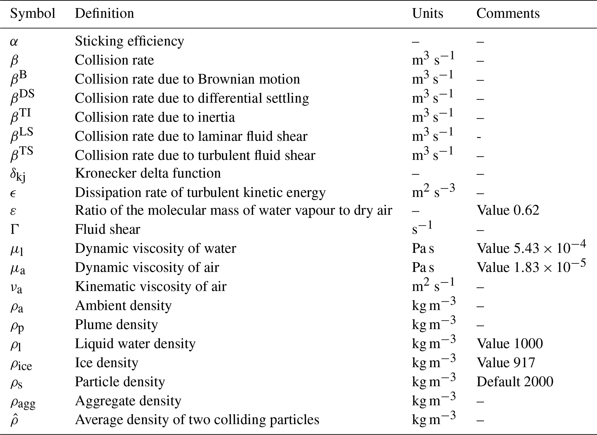
where j=l or ice. The meaning of the symbols used throughout are given in Tables 1 and 2. The entrainment rate depends on the ambient and plume densities, and when the plume is rising buoyantly is given as follows:
where ρp is the plume density, as follows:
where j=l or ice, and ue is the entrainment velocity, as follows:
Here two entrainment mechanisms are considered – one due to velocity differences parallel to the plume axis (us) and one due to the velocity differences perpendicular (un) to the plume axis. ks and kn are the entrainment coefficients associated with each respective entrainment mechanism (note that ks is given the symbol α and kn the symbol β in Devenish, 2013). The radial and cross-flow entrainment terms are raised to an exponent, f, which controls the relative importance of these two terms. Devenish et al. (2010) found that f=1.5 gave the best agreement with large eddy simulations of buoyant plumes in a crosswind and field observations, and we adopt this here.
Ice is produced whenever T<255 K, the critical temperature in the presence of volcanic ash, following Durant et al. (2008); Costa et al. (2010); Folch et al. (2016). It is assumed that there is no source liquid water or ice flux, given the high temperatures, and that there is no entrainment of ambient liquid water (only water vapour). Liquid water condensate and ice are formed whenever the water vapour mixing ratio (rv) is larger than the saturation mixing ratio (rs), which is determined using the Clausius–Clapeyron equation as follows:
where ε=0.62 is the ratio of the molecular mass of water vapour to dry air, pd is the dry ambient pressure, and es is the saturation vapour pressure, which, for liquid, is given by a modification of Tetens' empirical formula as follows (Emanuel, 1994, p. 117):
and, for ice, is given by the following (Murphy and Koop, 2005, p. 1558):
The mass fractions of water (nl) and ice (nice) can then be expressed as follows:
where nt is the total moisture fraction (), nl, ice is the mass fraction of either liquid water or ice, and nd is the dry gas fraction. It is assumed that any liquid condensate and ice that forms remains in the plume, and thus, the total water content is conserved.
The Smoluchowski coagulation equations are solved using the fixed pivot technique, which transforms a continuous domain of masses (while conserving mass) into a discrete space of sections, each identified by the central mass of the bin, i.e. the pivot. The growth of the aggregates is described by the sticking efficiency between the particles and their collision frequencies. The approach is computationally efficient but can be affected by numerical diffusion if the number of bins is too coarse compared to the population under analysis. The coupling of the fixed pivot technique with the one-dimensional buoyant plume model is applied at the level of the mass flux conservation equations. The mass flux is modified such that the mass fractions of the dry gas (nd), total moisture (nt, which is the mass fraction of vapour (nv) only, as neither liquid water or ice are entrained), and solid phases (ns) are treated separately, as follows:
where . As there is no entrainment or fallout of solids, Eq. (15) can be expressed as follows:
We assume a discretized GSD composed of Nbins, where the mass fractions of a given size (xi) are divided across a set of bins, such that . Assuming each size shares an amount of mass flux that is proportional to xi, Eq. (17) becomes the following:
where we used the linearity of the sum with respect to the derivative operator. This is the continuity equation for the mass flux of solids in the case of a steady-state process. The continuity equation can be seen as being a set of Nbins equations, one for each ith section, where aggregation is then taken into account by introducing source (Bi) and sink (Di) terms in the right-hand side of Eq. (18). The continuity equation for the ith bin then becomes the following:
In the fixed pivot technique, the source term Bi states that a given particle of the ith section can be created when the sum of the masses msum of two interacting particles k and j is between the pivots [i−1, i] and [i, i+1]. A fraction of msum is then proportionally attributed to the ith pivot, according to how close the mass msum is to mi. The redistribution of msum among the bins is done in such a way that the mass is conserved by definition. The sink term Di, on the other hand, is just related to the number of collisions and the sticking processes of the ith particles with all the other pivots available, and there is no need to redistribute mass. The fixed pivot technique applied to Eq. (19) then becomes the following:
where Ni is the number of particles of a given mass per unit volume, as follows:
Kk,j is the aggregation kernel between particles belonging to bins k and j, respectively, and δkj is the Kronecker delta function. As such, the Smoluchowski coagulation equations have been transformed into a set of ordinary differential equations which are solved for each bin representing the ith mass. The process of aggregation between two particles of mass mk and mj, at a given location s along the central axis of the plume, depends on the aggregation kernel (Kk,j), which can be expressed in terms of the sticking efficiency (αk,j) and the collision rate (βk,j) of the particles, as follows:
where αk,j is a dimensionless number between 0 and 1, which quantifies the probability of the particles successfully sticking together after a collision. βk,j describes the average volumetric flow of particles (cubic metres per second; hereafter m3 s−1) involved in the collision between particles k and j. We consider the following five different mechanisms (after Pruppacher and Klett, 1996, Costa et al., 2010, and Folch et al., 2016): Brownian motion (), interactions due to the differential settling velocities between the particles (), turbulent inertia (), and both laminar () and turbulent fluid shear ).
where dk and dj are the diameters, and Vk and Vj are the sedimentation velocities of the colliding particles, as follows:
where Cd is the drag coefficient, and Re is the Reynolds number, as follows:
and the sedimentation velocity is evaluated using an iterative scheme following Arastoopour et al. (1982). The laminar fluid shear is taken to be . The dissipation rate of turbulent kinetic energy per unit mass (ϵ) is constrained by the parameters controlling the large-scale flow, the magnitude of velocity fluctuations (about 10 % of the axial plume velocity), and the size of the largest eddies, which we take to be the plume radius, as follows (Textor and Ernst, 2004):
The total contribution from collisions due to each of the different mechanisms is represented by a linear superposition of each of the kernels (taking the maximum of the laminar shear and turbulent shear kernels):
The different collision mechanisms are evaluated at each position s along the central axis of the plume.
We assume that ash can stick together due to the presence of a layer of liquid water on the ash, following Costa et al. (2010). In this framework, the energy involved in the collision of particles k and j, identified from the relative kinetic energy of the bodies (i.e. rotations are not taken into account), can be parameterized in terms of the collision Stokes number (Stv) as follows:
which is a function of the average density of the two colliding particles (), the liquid viscosity (μl), and the relative velocities between the colliding particles (Ur), here approximated as follows:
Following a collision, particles stick together if the relative kinetic energy of the colliding particles is completely depleted by viscous dissipation in the surface liquid layer on the particles (Liu et al., 2000). The condition for this to occur is given by the following:
where h is the thickness of the liquid layer, and ha is the surface asperity or surface roughness (Liu et al., 2000; Liu and Lister, 2002). Unfortunately, this information is poorly constrained for volcanic ash. Instead, Costa et al. (2010) propose the following parameterization for the sticking efficiency:
using the experimental data of Gilbert and Lane (1994), which considered particles with diameters between 10 and 100 µm and set Stcr=1.3 and q=0.8 (see Fig. 12 in Gilbert and Lane, 1994, and Fig. 1 in Costa et al., 2010).
The influence of the ambient conditions, such as the relative humidity, on liquid bonding of ash aggregates still remains poorly constrained. Moreover, when trying to derive environmental conditions from one-dimensional plume models, it should be remembered that this description of a three-dimensional turbulent flow simply represents an average of the flow conditions and lacks details on local pockets of liquid water due to clustering of the gas mixture (Cerminara et al., 2016b). In these local regions, the concentration of water vapour can be high enough to reach the saturation condition and trigger the formation of liquid water. Furthermore, aggregation can occur even when the bulk value of the relative humidity is relatively low (Telling and Dufek, 2012; Telling et al., 2013; Mueller et al., 2016). As such, we allow sticking to occur in regions where the relative humidity is < 100 %, and liquid water is not yet present in the one-dimensional description of the plume, and we scale the sticking efficiency (αk,j) by the relative humidity as follows:
In the presence of ice, we assume that the sticking efficiency is constant, and , following Costa et al. (2010) and Field et al. (2006).
Table 1List of Latin symbols. Quantities with a superscript of 0 indicate values at the source.

To consider the influence of uncertainty on the source and internal model parameters on the simulated aggregated GSD, we have conducted a simple sensitivity study whereby the input parameters are varied one at a time. As such, we assess the difference between the simulated output using the set of default parameters (the control case) from a perturbed case. This approach assumes model variables are independent when considering the effects of each on model predictions.
For our case study, we consider the 2010 eruption of the Eyjafjallajökull volcano, Iceland (location 63.63∘ lat, −19.62∘ long; summit height 1666 m a.s.l. – above sea level), between 4 and 8 May 2010. We use the time profile of plume heights given in Webster et al. (2012), which are based on radar data, pilot reports, and Icelandic coastguard observations. Meteorological data, used by the aggregation scheme and NAME simulations, are from the global configuration of the Unified Model (UM) which, for this period, had a horizontal resolution of ∼ 25 km (at mid-latitudes) and a temporal resolution of 3 h. Figure 1 shows the relative humidity (RH), temperature (T), and mixing ratios of liquid water (nl/nd), water vapour (nv/nd), and ice (ni/nd) with height along the plume axis at different times during the eruption. Note that the maximum height of the modelled plume axis, when the plume is bent over as in this case, is the maximum observed plume height minus the plume radius (Mastin, 2014; Devenish, 2016). At 19:00 UTC on 04 May 2010, the maximum observed plume height is 7000 m a.s.l., liquid water starts to form at 4122 m a.s.l., but no ice forms in the plume. At 12:00 UTC on 5 May 2010, the observed maximum plume height is lower, reaching just 5500 m a.s.l., liquid water is present from 3684 m a.s.l., and again no ice is formed. However, at 13:00 UTC on 6 May 2010, no liquid water forms in the plume, only ice, which is present from 5582 m a.s.l., and the maximum observed plume height is 10 000 m a.s.l. At 12:00 UTC on 7 May 2010, the maximum observed plume height is 5500 m a.s.l., and there is neither liquid water nor ice in the plume – only water vapour.
The control values used for the source and internal model parameters in the aggregation scheme are given in Table 3, along with the range of values for each parameter considered in the sensitivity study. Values are based on the existing literature, and the sources used are also listed in Table 3. The scheme is initialized with a GSD with a uniform distribution of mass across 14 bins, representing particles with diameters ranging from 1 µm to 16 mm. Bins are defined on the phi scale, where the phi diameter is calculated as the negative logarithm to the base 2 of the particle diameter in millimetres (Krumbein, 1938). The mass is distributed uniformly across the bins, such that 50 % is on grains with diameter ≤ 125 µm and 36 % of the mass is on grains with diameter ≤ 32 µm (Fig. 2). The output-aggregated GSD at the top of the plume, defined as the point at which Wp=0, is assessed. Given the nature of the Smoluchowski coagulation equations, the aggregation scheme does not track explicitly the mass fraction of aggregates versus single grains within a given bin size. Instead, we consider how the mode of the output-aggregated GSD varies and compare the mass fraction on particles with diameter ≤ 32 µm (m32), which predominantly lose mass to larger aggregates, for each sensitivity run. First, we consider how the aggregated GSD varies as conditions within the plume change over time given the local meteorological and eruption conditions (plume height). Figure 2 shows the output aggregated GSDs, for the same times as the plume conditions shown in Fig. 1, compared to the input GSD. We find that, in all the cases considered, the mode of the aggregated GSD is always the same, with most of the mass now residing in the 125–250 µm bin. When particles spend more time in the presence of liquid water, m32 decreases slightly; m32=32 % at 19:00 UTC on 4 May 2010 when liquid water is present from 4122 m a.s.l., but m32=33 % at 12:00 UTC on 5 May 2010 when liquid water is only available over a more limited depth (Fig. 2a, b). Aggregation still occurs when there is only ice present and no liquid water (6 May 2010 at 13:00 UTC; Fig. 2c) and when there is no ice or liquid water present (12:00 UTC on 7 May 2010; Fig. 2d).

Figure 1Mixing ratios of water vapour (nv/nd), liquid water (nl/nd), and ice (nice/nd) with height along the buoyant plume axis, for the eruption of Eyjafjallajökull volcano between 4 and 7 May 2010. Also shown are the relative humidity and temperature. Note the variation in axis scales. The maximum height of the modelled plume axis, when the plume is bent over as in this case, is the maximum observed plume height (provided in the figure titles) minus the plume radius.
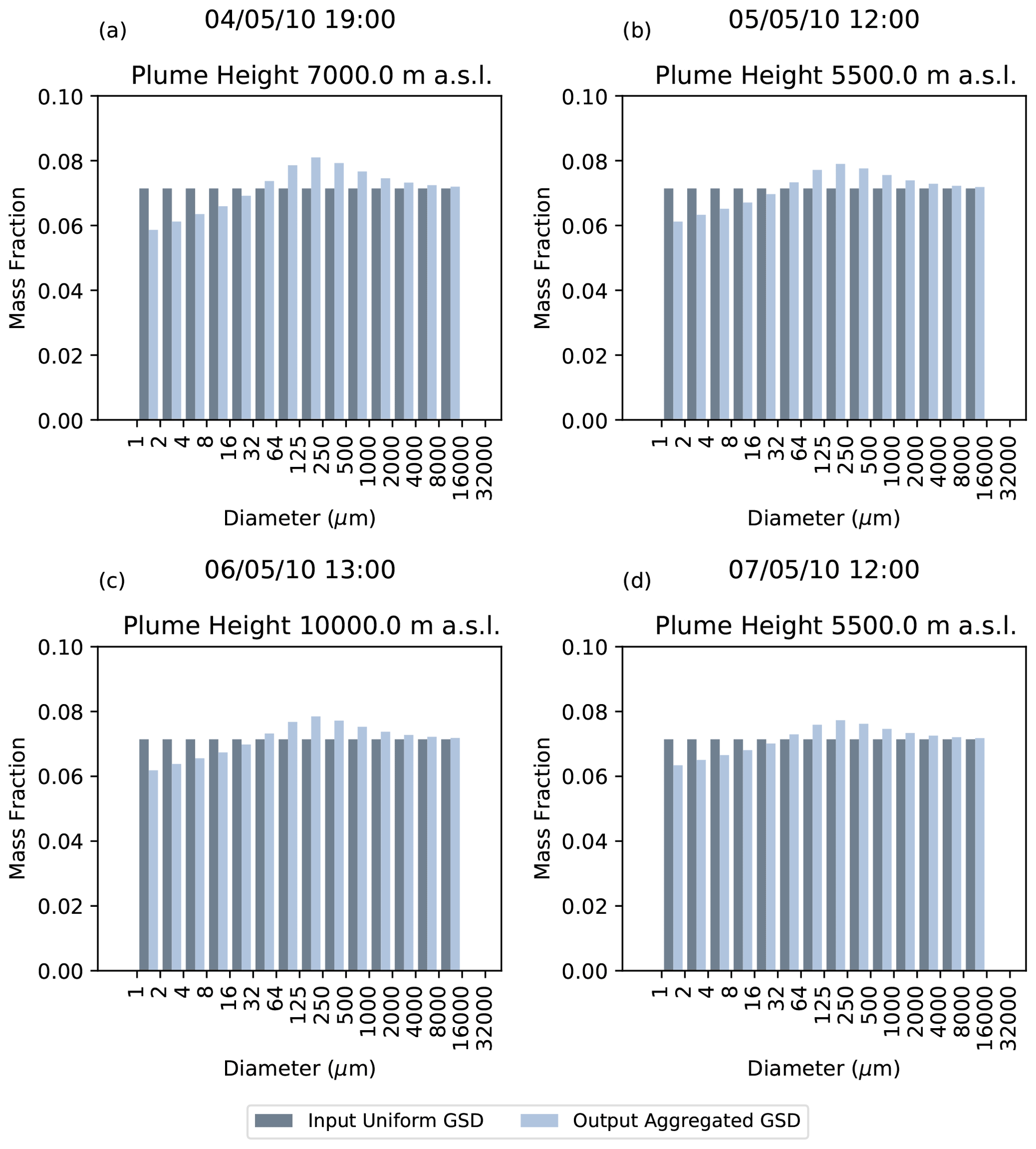
Figure 2Modelled aggregated GSDs corresponding to the times and phase conditions shown in Fig. 1. The aggregation scheme is initialized with a GSD with a uniform distribution of mass, as indicated by the dark blue bars.
Table 3Model variables used in the aggregation scheme to represent the eruption conditions. The control values listed for each parameter are based on the defaults used in the existing literature. The range of parameter values considered in the sensitivity study are also given.

Table 4Properties of the simulated aggregated GSD from the model sensitivity runs. The output is for 19:00 UTC on 4 May 2010. Using control values (Table 3), the mode is at 125–250 µm and m32 32 %.
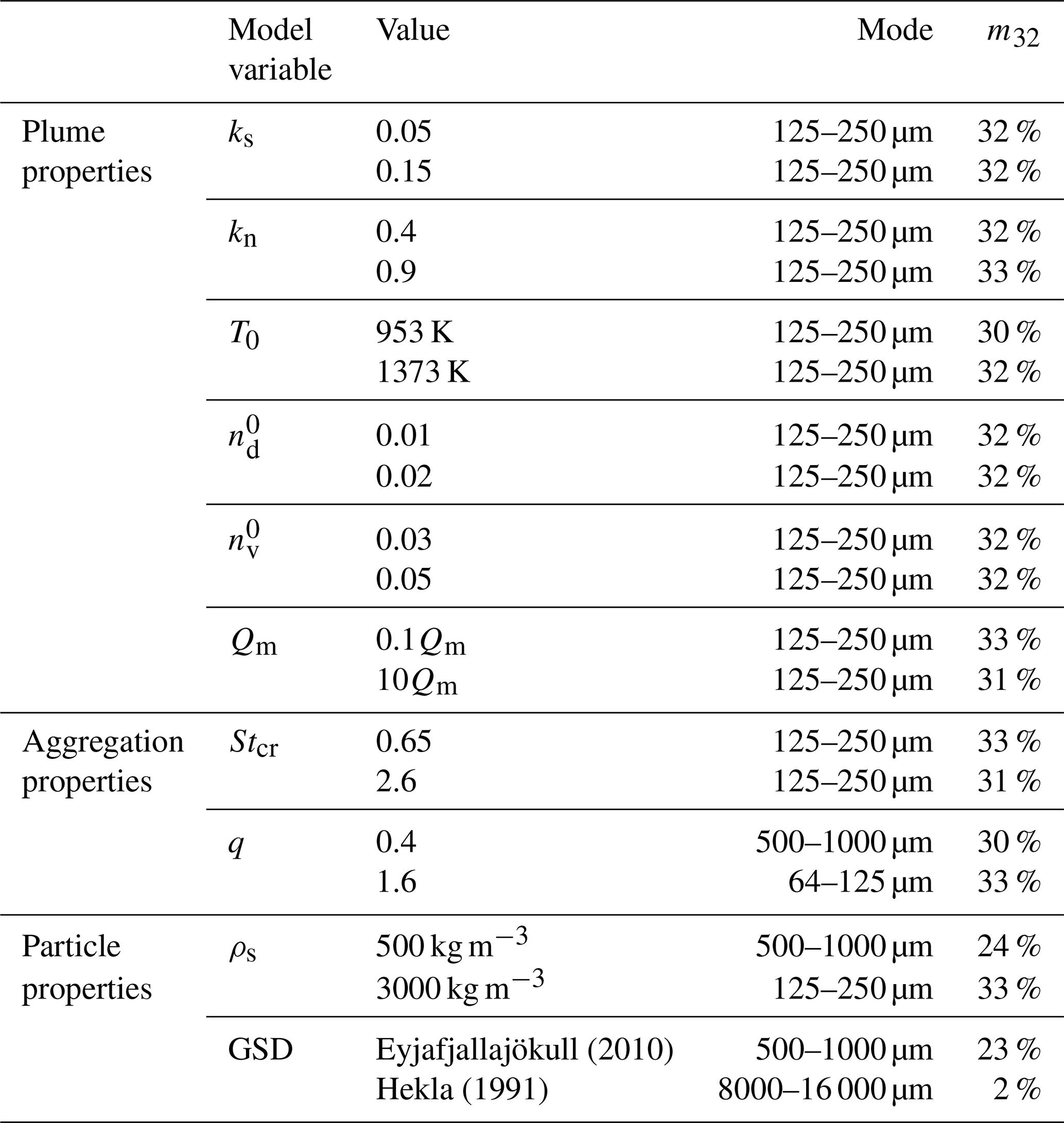
The mode and m32 of the simulated aggregated GSD for each sensitivity run output at 19:00 UTC on 4 May 2010 are listed in Table 4. Using the control parameters, the mode of the aggregated GSD lies at 125–250 µm, and m32 is 32 % at this time (cf. Fig. 2a). The aggregation scheme is sensitive to the values assigned to the sticking parameters (Stcr and q) and the parameters which define the particle characteristics, the input GSD, and the particle density (note that here all model particles are assigned the same density; as such, ). Figure 3 shows how the cumulative distribution of the aggregated GSD changes as these parameters are varied within their known ranges. The parameters used to set the sticking efficiency between the particles (Stcr and q) are currently poorly understood and, therefore, under-constrained. Figure 3a–b show the aggregated GSD when Stcr and q are varied by a factor of 2. When q=0.4, m32 is 30 %, and the mode of the aggregated GSD moves to 500–1000 µm; when q=1.6, the mode lies at 64–125 µm, and for Stcr in the range 0.65–2.6, m32 varies from 31 %–33 %. When particles have a (low) density of 500 kg m−3, m32 is 24 %, and the modal bin is 500–1000 µm (Fig. 3c). We find that, when using a relatively coarse input GSD (from the eruption of Hekla in 1991), there is very little aggregation, and there is no change in m32 or the modal grain size from the input GSD (Fig. 3d). Whereas, when using the Eyjafjallajökull (2010) GSD, which is much finer, the mode of the aggregated GSD is shifted to larger sizes. Output from the sensitivity runs for other times during the eruption (corresponding to those in Fig. 2) are provided in the Supplement and show the same behaviour (Figs. S1–S3).
The aggregated GSD shows little sensitivity to the model values assigned to define the plume conditions within the ranges investigated, namely the entrainment parameters (ks and kn), the initial mass fraction of dry gas and water vapour (,), the plume temperature at the source (T0), or the source mass flux (Qm; see Table 4 and Figs. S4–S7). When we consider that the mass flux may have an order of magnitude uncertainty, and vary the input mass flux to the aggregation scheme by a factor of 10, m32 varies by just 1 %.

Figure 3Sensitivity of the output aggregated GSD to the sticking efficiency parameters, (a) Stcr and (b) q, and the physical characteristics assigned to the particles, (c) particle density ρs, and (d) input GSD. Output is for 19:00 UTC on 4 May 2010, and the plume height is 7000 m a.s.l. (cf. Fig. 2a). Note that the blue lines represent simulations using the control values, and AGSD is the aggregated GSD.
3.1 Scale analysis of the collision kernel
To gain insight into the dependence of the aggregation kernel (Kk,j) on the critical Stokes number (Stcr), the parameter (q), the size of the particles (dk,j), and their density (ρs), we performed a scale analysis of the collision rate (βk,j) and sticking efficiency (αk,j), the details of which are provided in Appendix A. All of the parameters, other than the one being varied, are kept fixed at the control (default) values listed in Table 3.
First, we consider how the behaviour of the collision rate (βk,j) changes as the particle size and density varies. Figure 4 shows the variation in the collision rate between two particles of the same fixed density, where the diameter of one of the colliding particles (dj) is kept fixed (diameters of 10, 100, and 1000 µm are considered) and the diameter of the second particle (dk) is allowed to vary between 1 and 10 000 µm, consistent with the GSD of the tephra considered in this study (Table 4). For typical values of each of the parameters that occur in the different kernels considered in the collision rate equation (Eq. 33), and assuming Stokes drag, the scale analysis in Appendix A shows that the collision rate is dominated by differential settling () when dk≫dj or dk≪dj. As it is the larger particle which determines the collision rate in these limiting cases, then for dk≪dj the collision rate is effectively constant; the scale analysis gives the correct order of magnitude for βk,j in these cases. When dk≫dj, then, to leading order, the collision rate increases to the fourth power of the diameter of the colliding particle () and is independent of dj. However, Fig. 4 shows that when dk≳102 µm, βk,j departs from this power law when the Reynolds-number-dependent terminal velocity is used (Eqs. 29–31). When dk=dj, then the collision rate is dominated by shear, except for the very smallest particles (of the order of 1 µm) when it is dominated by Brownian motion. The scale analysis gives the correct order of magnitude for these cases and explains the kinks seen in Fig. 4, when dk=dj, and why they become sharper as dj increases. When the assumption of constant ρs is relaxed, it is easily seen that βk,j depends linearly on ρs (through and ) for dk≠dj; when dk=dj, the collision rate is independent of ρs.
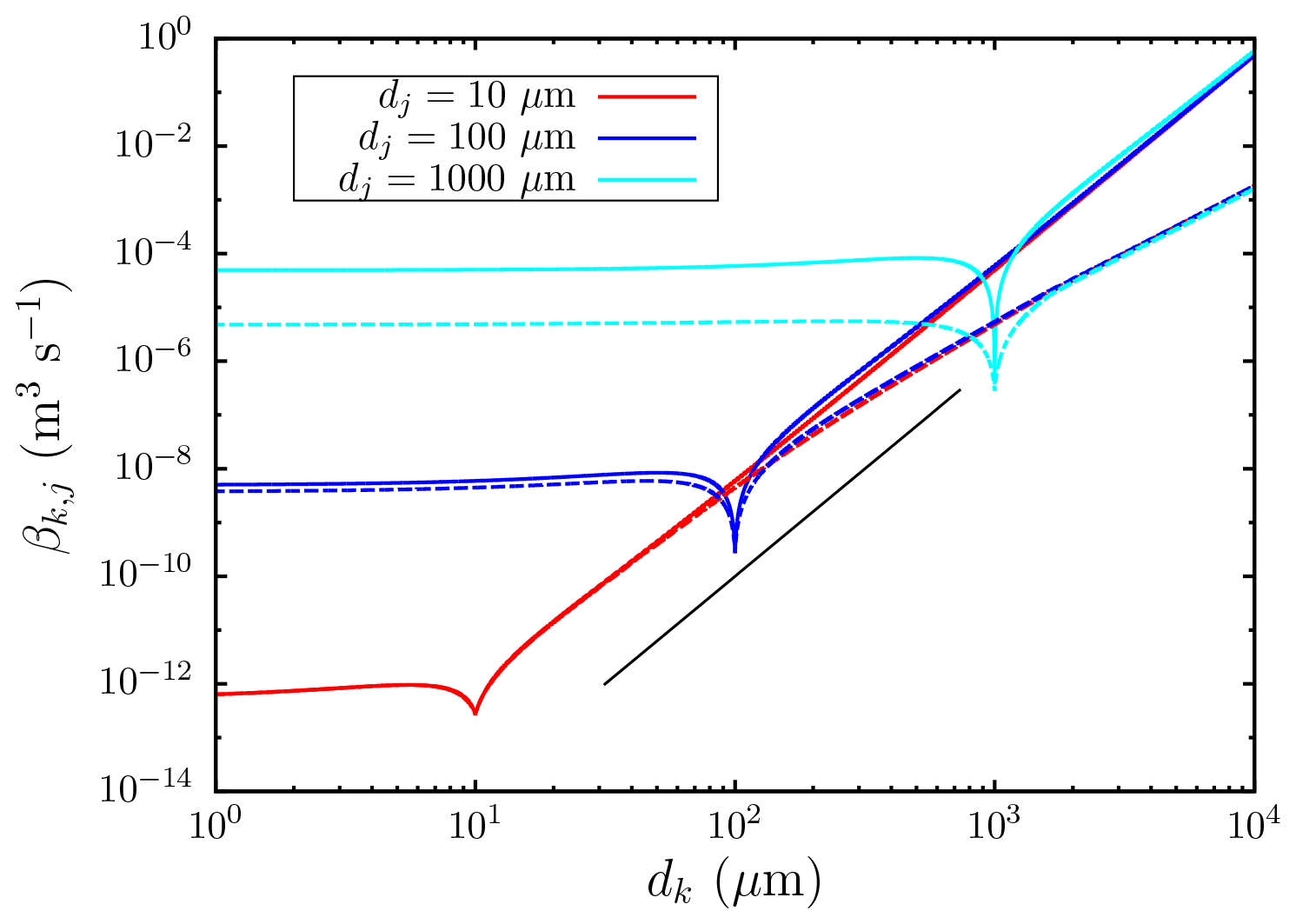
Figure 4The variation in the collision rate (βk,j) between particles as the size of the particle dk varies for three values of dj. The solid lines are calculated with Stokes terminal velocity, and the dashed lines are calculated with the terminal velocity given by Eqs. (29)–(31). The black line is proportional to .
We now turn to the sensitivity of the sticking efficiency (αk,j) to the critical Stokes number (Stcr), the sticking parameter (q), and the density of the particles (ρs). It follows immediately from Eq. (37) that increasing Stcr increases the range of values of the collision Stokes number (Stv) for which coalescence can occur. When Stv≪Stcr, , and coalescence is almost certain, q has the effect of enhancing or reducing the effect of , with q>1 reducing the effect in this limit and so increasing the sticking efficiency further and vice versa for q<1. When Stv≫Stcr, , and there is effectively no coalescence; q>1 has the effect of increasing the value of relative to its value with q=1 and, hence, reducing the sticking efficiency still further, whereas the converse applies when q<1. How the sticking efficiency depends on diameter is determined by the dependence of Stv on dj and dk, and this is given by the scale analysis in Appendix A. When dk=dj, Stv (via Ur, as given by Eq. 35) is dominated by shear (), except for the smallest particles (of the order of 1 µm) when it is dominated by Brownian motion (). When dk≠dj, Stv is dominated by differential settling; for dk≪dj, we find that , whereas, for dk≫dj, we have . It is the size of this term relative to Stcr which determines whether αk,j is close to one or not.
Figure 5 shows the sensitivity of the sticking efficiency (αk,j) to the critical Stokes number (Stcr), the sticking parameter (q), and the density of the particles (ρs) for three fixed values of dj (10, 100, and 1000 µm). Figure 5 clearly shows the asymmetry in the dependence of αk,j on dj and dk, as highlighted above. Figure 5a–c show the sensitivity of αk,j to the critical Stokes number (Stcr) as follows: as Stcr increases, αk,j increases towards one for fixed dj and dk indicating, as expected, a greater propensity for the particles to coalesce. As dj increases, αk,j tends to decrease, indicating the increasing importance of the ratio in the evaluation of αk,j. Figure 5d–f show the sensitivity of αk,j to the parameter q which acts to alter the shape of the sticking matrix. There is more variation with q than with Stcr; because q appears in αk,j as an exponent, a change in the value of q is not simply a multiplicative change as it is with a change in the value of Stcr. Figure 5g–i show the sensitivity of αk,j to ρs. This occurs because to leading order and so αk,j decreases with increasing ρs.
Figure 6 shows the variation in the collision kernel, (Eq. 23), with Stcr, q, and ρs. It is immediately clear that, while the sticking efficiency tends to increase when particles are small (Fig. 5), this effect is negated by the reduction in the collision rate (Fig. 4) for particles of the same size. The net effect is that the largest values of the collision kernel tend to be found for the particles with the largest diameters (Fig. 6). The largest range of values occurs for the smallest value of dj and vice versa. This reflects the dominance of differential settling in the collision kernel.
The collision kernel inherits its sensitivity to Stcr and q from the sticking efficiency, αk,j. Figure 6 shows that the variation in Kk,j with Stcr (over the range of values shown in Fig. 6a–c) is smaller than the variation in Kk,j with ρs (Fig. 6g–i) and that both of these are smaller than the variation in Kk,j with q (Fig. 6d–f). For a given value of dk, the value of Kk,j increases with increasing Stcr but decreases with increasing ρs. Figure 6d–f show that the variation with q is more complicated, but the largest values of Kk,j occur for the smallest values of q (for a given value of dk). This explains why the mode of the aggregated GSD in Fig. 3 shifts to larger diameters with increasing Stcr, decreasing q or ρs (see also Table 4). The behaviour of the sticking efficiency (αk,j), collision rate (βk,j) and its product, the collision kernel (Kk,j), with respect to changes in Stcr, q, and ρs explains why there is less variation in the aggregated GSD with Stcr compared with q and ρs. However, this behaviour cannot explain all the variation in the aggregated GSD with ρs, which is much larger than that with either Stcr or q. The additional factor is explained by the fact that the particle number density for a given size bin, Ni, increases with decreasing ρs, since mi is proportional to ρs (Eq. 22).
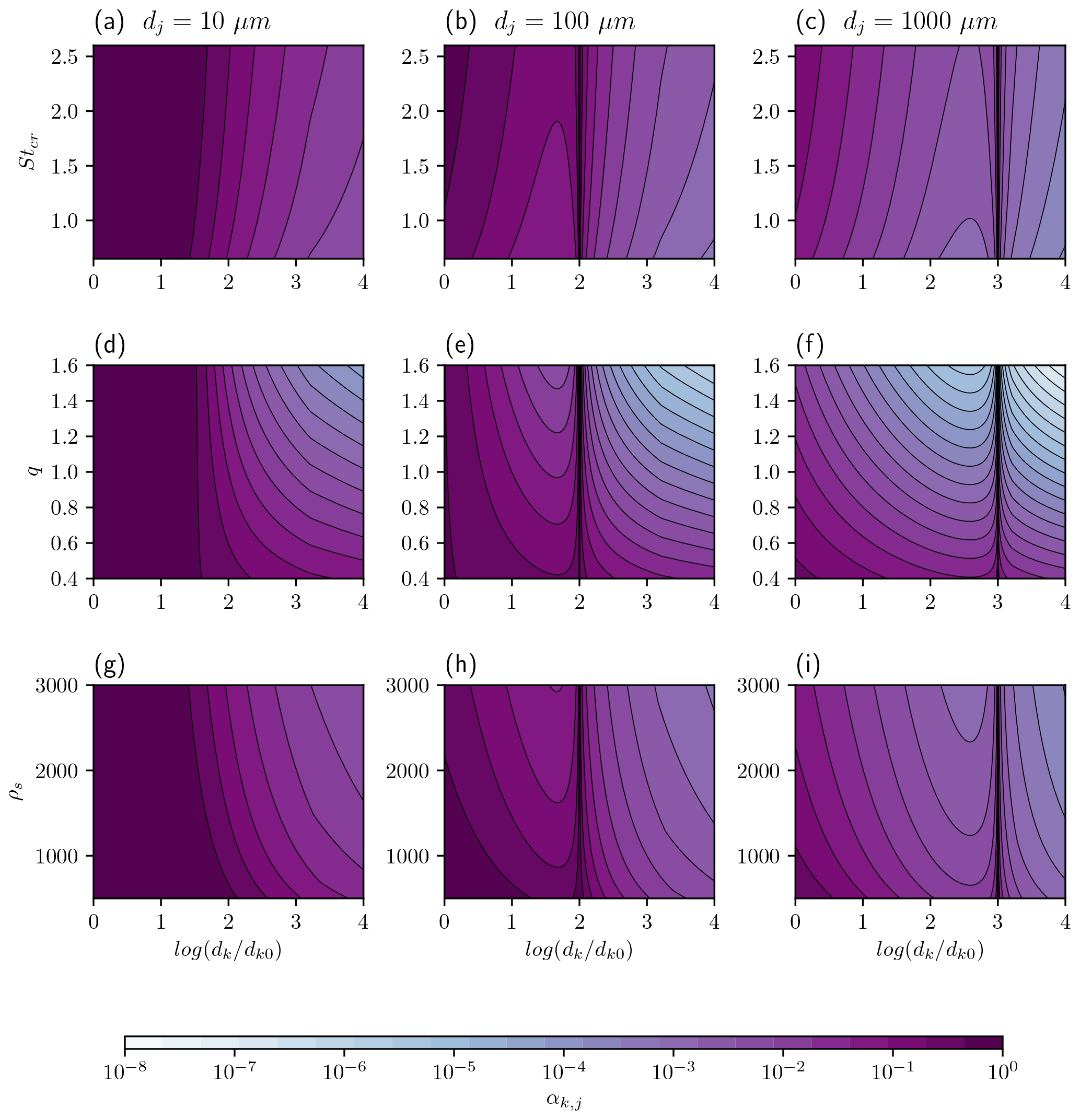
Figure 5The variation in sticking efficiency (αk,j), with Stcr (a–c), q (d–f), and ρs (g–i) for three fixed values of dj, i.e. dj=10 µm (a, d, g), dj=100 µm (b, e, h), and dj=1000 µm (c, f, i). The terminal velocity is calculated using Eqs. (29)–(31). The diameter dk0=1 µm.
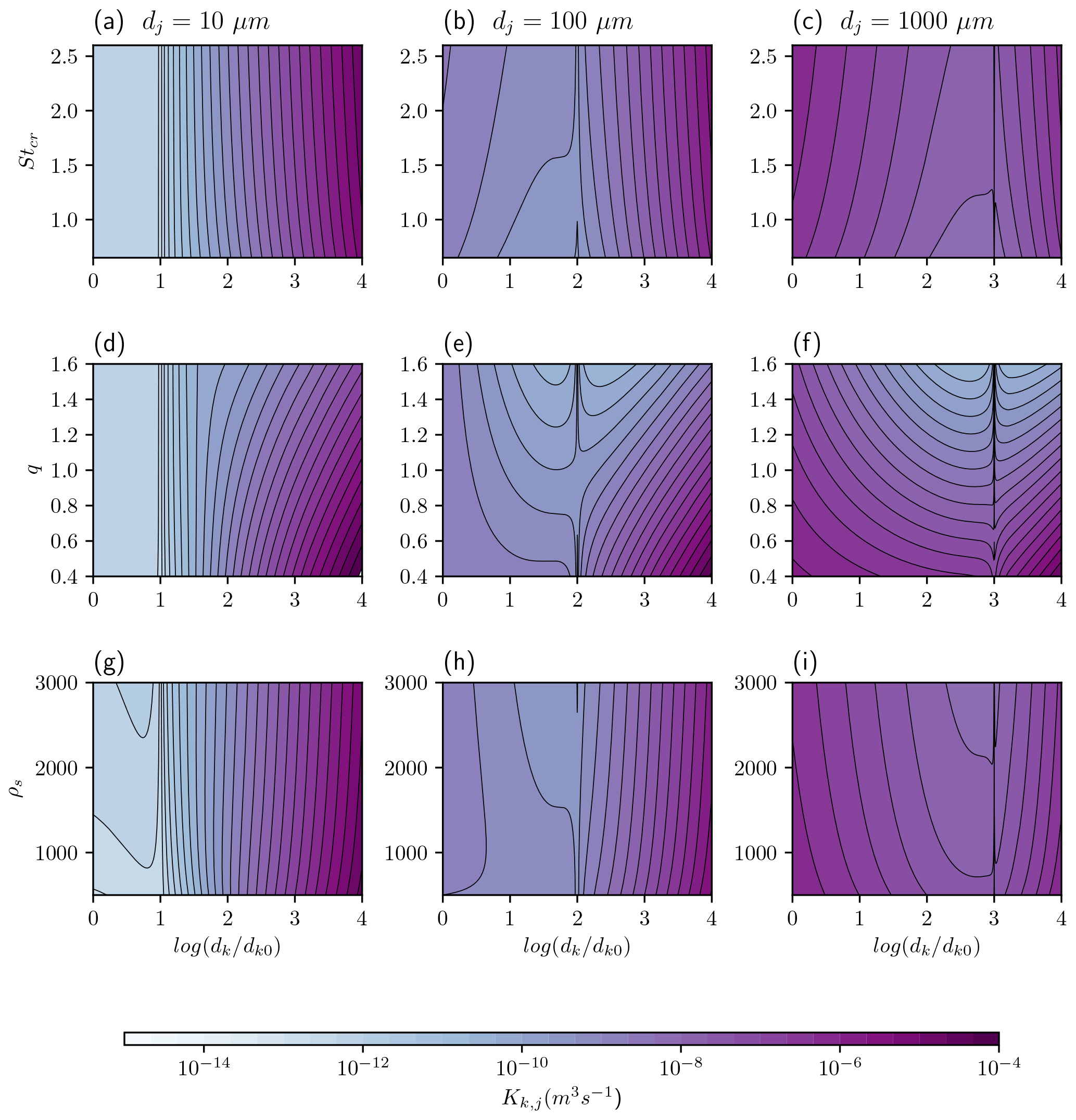
Figure 6The variation in the collision kernel (Kk,j) with Stcr (a–c), q (d–f), and ρs (g–i) for three fixed values of dj, i.e. dj=10 µm (a, d, g), dj=100 µm (b, e, h), and dj=1000 µm (c, f, i). The terminal velocity is calculated using Eqs. (29)–(31). The diameter dk0=1 µm.
We now investigate the impact of representing aggregation on dispersion model simulations of the distal ash cloud from the eruption of the Eyjafjallajökull volcano in 2010. We consider the period between 4 and 8 May 2010, as we have measurements of the GSD and density of the non-aggregated grains for this time (Bonadonna et al., 2011). The aggregation scheme is initialized with the measured GSD of the non-aggregated tephra, with diameters between 1 µm and 8 mm, provided in Bonadonna et al. (2011), which is based on both deposit and satellite measurements. Figure 7 shows the output aggregated GSD at 19:00 UTC on 4 May 2010. Following aggregation, there are fewer grains with diameters ≤16 µm, but the mode of the distribution remains at 500–1000 µm. Furthermore, the total fraction of mass on ash with diameters ≤125 µm has changed very little; prior to aggregation, 41 % of the total mass is represented by ash with diameters ≤125 µm. This is reduced to just 39 % following aggregation. The density distribution of the non-aggregated Eyjafjallajökull grains is also shown; densities range from 2738 to 990 kg m−3 for this size range (Bonadonna and Phillips, 2003; Bonadonna et al., 2011). The aggregation scheme is coupled to NAME, such that it uses the output-aggregated GSD at the top of the plume and the mass eruption rate (MER) calculated from the buoyant plume scheme, which is initialized with the observed plume heights, at every time step. When NAME is used by the London VAAC, it is initialized with small particles which are expected to remain in the atmosphere and contribute most to the distal ash cloud (Beckett et al., 2020; Osman et al., 2020). We follow this approach in our simulations; we use the aggregated GSD up to 125 µm, and the MER is scaled to represent the mass on these grains only. For example, at 19:00 UTC on 4 May 2010, 39 % of the total mass erupted is released over the seven bins representing ash with diameters ≤125 µm (Fig. 7). The exact diameter of each model particle is allocated such that the log of the diameter is uniformly distributed within each size bin. These model particles are then released with a uniform distribution over the depth of the modelled (bent-over) plume. See Devenish (2013, 2016) for details of how the plume radius (depth) is constrained. The set-up of the NAME runs is given in Table 5, and we use the control internal model parameters in the aggregation scheme (Table 3).
Figure 8a shows the modelled 1 h averaged total column mass loadings in the ash cloud at 00:00 UTC on 5 May 2010, 24 h after the release start, using the measured GSD and density distribution of the non-aggregated Eyjafjallajökull particles. In comparison, Fig. 8b shows the modelled plume using the time-varying aggregated GSD. As the density of the Eyjafjallajökull aggregates is not known, the measured density distribution of the single grains is applied. Current regulations in Europe state that airlines must have a safety case accepted to operate in ash concentrations greater than g m−3. We assume a cloud depth of 1 km and consider the area of the ash cloud with mass loadings > 2 g m−2 to compare the differences in the modelled areas which are significant for aircraft operations. Using the aggregated GSD, the extent of the ash cloud is only slightly smaller; it is reduced by just ∼ 2 %, reflecting the slight increase in the fraction of larger (aggregated) grains in the ash cloud, which have a greater fall velocity and, hence, shorter residence time in the atmosphere.
However, it is expected that porous aggregates, specifically cored clusters which consist of a large core particle (> 90 µm) covered by a thick shell of smaller particles (Brown et al., 2012; Bagheri et al., 2016) may have lower densities than single grains of ash of equivalent size (Bagheri et al., 2016; Gabellini et al., 2020; Rossi et al., 2021). Figure 9 shows the modelled ash cloud when we assume that the aggregates have densities of 1000 and 500 kg m−3 (Taddeucci et al., 2011; Gabellini et al., 2020; Rossi et al., 2021). As the aggregation scheme does not track explicitly the mass fraction represented by aggregates versus single grains for a given size bin, we must also make an assumption about how much of the mass released is represented by aggregates with lower density. Here we consider the case where 25 %, 50 %, and 75 % of the mass on each size bin, for ash with diameters ≤125 µm, is represented by aggregates. Assigning a lower density to the aggregates reduces their fall velocity, and the extent of the simulated ash cloud increases. If we assume that 75 % of the mass of ash ≤125 µm is represented by aggregates, then, when they are assigned a density of 1000 kg m−3, the simulated ash cloud with mass loadings >2 g m−2 is 152 308 km2. This increases to 159 966 km2 when they are assigned a density of 500 kg m−3. Figure 10 shows the relative increase in the area of the ash cloud with concentrations >2 g m−2 as a function of the mass fraction of aggregates in the ash cloud and their density. The circle with a diameter of 1 represents the extent of the modelled cloud when aggregation is not considered (area 143 459 km2). The largest modelled ash cloud is ∼ 1.1 times bigger. This is achieved when we use the aggregated GSD, assign the aggregates a density of 500 kg m−3, and assume that aggregates constitute 75 % of the total mass released in NAME (ash ≤125 µm).

Figure 7The GSD of the Eyjafjallajökull (2010) non-aggregated tephra (dark grey bars; from Bonadonna et al., 2011), used to initialize the aggregation scheme, and the modelled aggregated GSD at the top of the plume (light grey bars), at 19:00 UTC on 4 May 2010. The density distribution of the non-aggregated particles, taken from Bonadonna et al. (2011), is also shown.
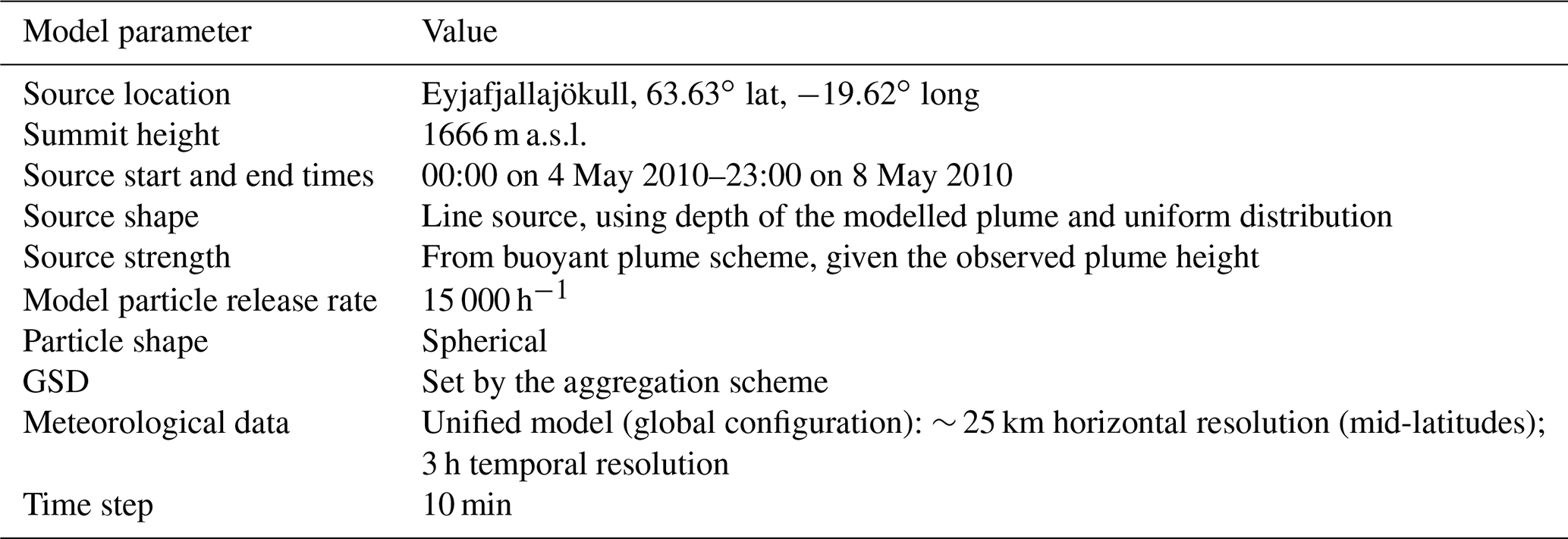
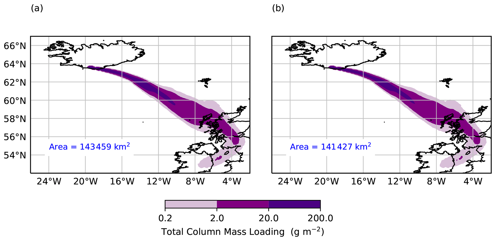
Figure 8Modelled 1 h averaged total column mass loadings of the Eyjafjallajökull ash cloud at 00:00 UTC on 5 May 2010, using (a) the measured GSD of the non-aggregated ash and (b) the time-varying aggregated GSD. The measured density distribution of the non-aggregated ash grains is applied in both cases. The area of the ash cloud with mass loadings >2 g m−2, which is significant for aircraft operations, is shown.
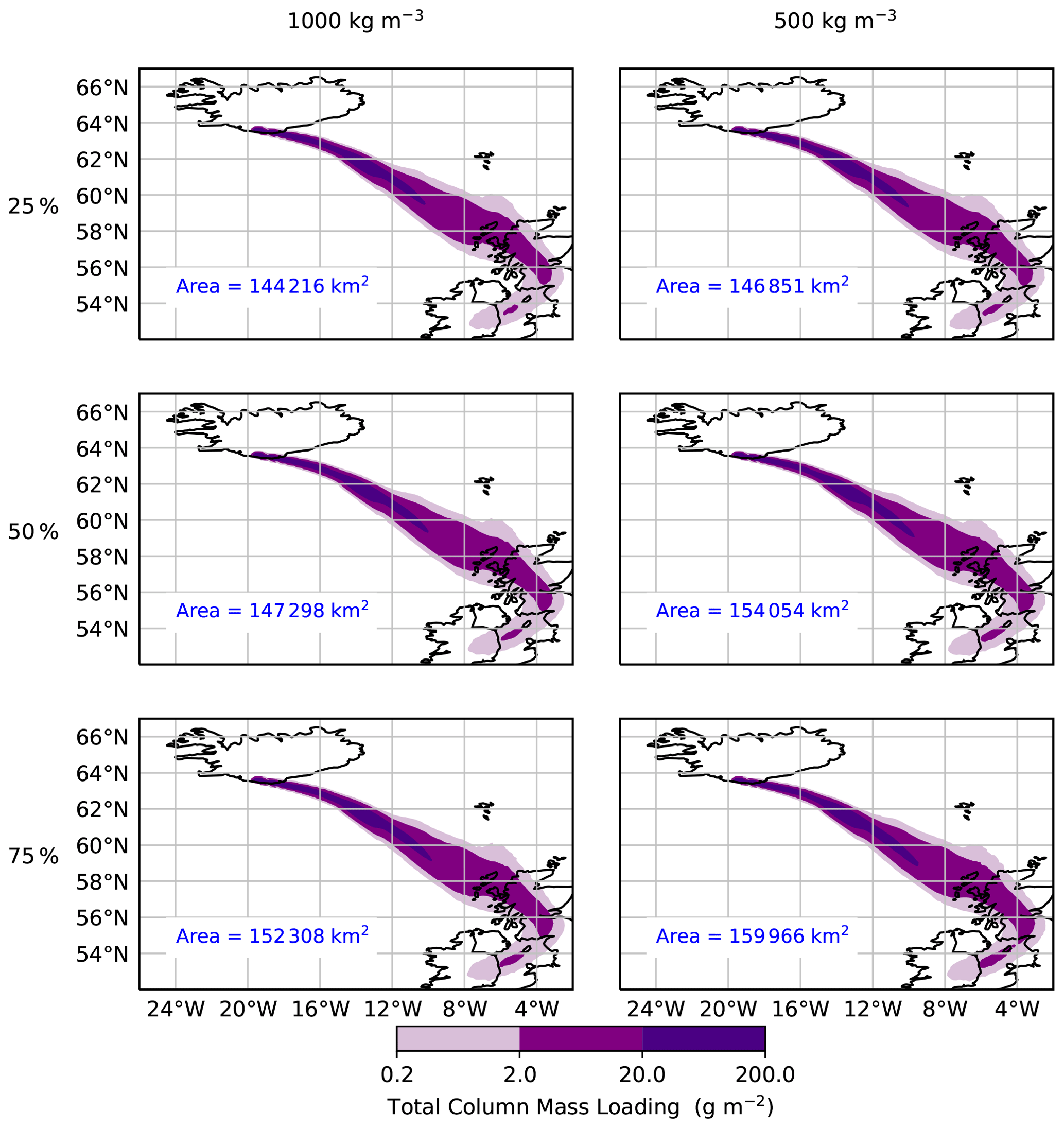
Figure 9Modelled 1 h averaged total column mass loadings of the Eyjafjallajökull ash cloud at 00:00 UTC on 5 May 2010 when 25 %, 50 %, and 75 % of the mass is on aggregates with densities of 1000 and 500 kg m−3. The area of the ash cloud with mass loadings >2 g m−2, which is significant for aircraft operations, is shown.
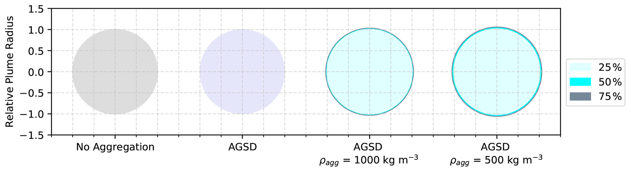
Figure 10Relative areas of the Eyjafjallajökull ash cloud with concentrations >2 g m−2 at 00:00 UTC on 5 May 2010. The area of the ash cloud, when aggregation is not considered, has a relative radius of 1. The modelled areas, using aggregated GSDs when 25 %, 50 %, and 75 % of the mass released is assumed to be on aggregates with a density of 1000 and 500 kg m−3, are compared.
We have integrated an aggregation scheme into the atmospheric dispersion model NAME. The scheme is coupled to a one-dimensional buoyant plume model and uses the fixed pivot technique to solve the Smoluchowski coagulation equations to simulate aggregation processes in an eruption column. The time-evolving aggregated GSD at the top of the plume is provided to NAME as part of the source conditions. This represents the first attempt at modelling explicitly the change in the GSD of the ash due to aggregation in a model which is used for operational response, as opposed to assuming a single aggregate class (Cornell et al., 1983; Bonadonna et al., 2002; Costa et al., 2010). Our scheme predicts that mass is preferentially removed from bins representing the smallest ash (≤64 µm). This agrees well with field and laboratory experiments which have also observed that aggregates mainly consist of particles <63 µm in diameter (Bonadonna et al., 2011; James et al., 2002, 2003). This suggests that aggregation will be more prevalent when large quantities of fine ash are generated by the eruption.
Previous sensitivity studies of dispersion model simulations of volcanic ash clouds have highlighted the importance of constraining the GSD of ash for operational forecasts, as this parameter strongly influences its residence time in the atmosphere (Scollo et al., 2008; Beckett et al., 2015; Durant, 2015; Poret et al., 2017; Osman et al., 2020; Poulidis and Iguchi, 2020). Here we show that the modelled aggregated GSD is also sensitive to the GSD, and the density, of the non-aggregated particles at the source. When the scheme is initialized with a coarse GSD, there are fewer particles per unit volume (lower number concentrations) within the plume, and aggregation is reduced. When particle densities are low, for the same mass flux, there are higher number concentrations and hence more aggregation.
Dispersion model simulations are influenced by the interplay between the size and density distributions assigned to the particles. Aggregates can have higher fall velocities than the smaller single grains of which they are composed and, therefore, act to reduce the extent and concentration of ash in the atmosphere (Rossi et al., 2021). However, porous aggregates can also have lower densities than the single grains, and this can act to raft ash to much greater distances (Bagheri et al., 2016; Rossi et al., 2021). In our case study of the Eyjafjallajökull 2010 eruption, we found that, although mass was lost from bins representing smaller grain sizes, the mode of the aggregated GSD did not differ from the source GSD of the erupted non-aggregated particles; for example, the output aggregated GSD at 19:00 UTC on 4 May 2010 has lost mass from ash ≤16 µm but the mode remains at 64–125 µm (Fig. 7).
Our dispersion model set-up in this study reflects the choices used by the London VAAC; as such we examine the transport and dispersion of ash with diameters ≤125 µm, and we consider the implications for the modelled extent of the ash cloud with mass loadings of significance to the aviation industry. We found that using the time-varying aggregated GSD to initialize our dispersion model, rather than the size distribution of the single grains, had little impact on the simulated ash cloud. When we considered that aggregates may have (lower) densities of 1000 and 500 kg m−3 and make up 25 %–75 % of the total mass of the simulated aggregated GSD, we found that the area of the ash cloud with concentrations significant for aircraft operations (>2 g m−2) varied by a factor of just ∼ 1.1. Previous studies, which have considered the sensitivity of dispersion model forecasts of volcanic ash clouds to the density distribution of the ash, have also suggested that simulations are relatively insensitive to this parameter (Scollo et al., 2008; Beckett et al., 2015). In fact, in this case, the modelled ash cloud is more sensitive to the input GSD of the non-aggregated particles at the source than due to any change to the GSD or density due to aggregation. Osman et al. (2020) compared NAME simulations initialized with the default GSD used by the London VAAC (which is relatively fine) and the published GSD of ash from the 1991 eruption of Hekla (which is much coarser). They found that simulations of the extent of the Eyjafjallajökull ash cloud in 2010 with concentrations >2 g m−2 varied by a factor of ∼ 2.5.
It should be remembered that operational forecasts are also sensitive to other eruption source parameters needed to initialize dispersion model simulations. Dioguardi et al. (2020) found that, given the uncertainty on the MER, forecasts of the area of the Eyjafjallajökull ash cloud with concentrations g m−3 varied by a factor of 5. When generating operational forecasts, uncertainty on the plume height, vertical distribution, MER, and GSD of the non-aggregated particles at the source could, therefore, outweigh any error associated with not representing aggregation processes.
The grain size distribution of the non-aggregated Eyjafjallajökull tephra, determined using ground sampling and satellite retrievals, indicated that ∼ 20 wt % of the total mass erupted was ash with diameters ≤16 µm (Fig. 7; Bonadonna et al., 2011). Given their relatively low fall velocities, ash of this size can travel significant distances, e.g. >3000 km, given the plume heights and meteorological conditions during the Eyjafjallajökull eruption (Beckett et al., 2015). However, Bonadonna et al. (2011) observed that ∼ 50 % of this very fine ash was deposited on land in Iceland (within 60 km from the vent) and, therefore, must have fallen out quicker than their settling velocity would allow, due to either particle aggregation or gravitational instabilities or both. Our simulated aggregated GSDs at the top of the eruption column have formed very few larger grains; as such, 18 % of the total mass erupted is still represented by grains with diameters ≤16 µm. The small mass reduction in the fraction of grains with diameters ≤16 µm predicted by our model could be due to various limitations in our scheme and approach, for example, a poor description of dry aggregation, of regions of water saturation, and of particle collision in turbulent flows. We now discuss these limitations in detail.
5.1 Limitations
To be considerate of the computational costs for operational systems, we have limited aggregation processes to the eruption column only. However, it is likely that, while ash concentrations remain high, aggregation will continue in the dispersing ash cloud. As we do not represent electric fields in our scheme, we are also unable to explicitly simulate aggregation through electrostatic attraction (Pollastri et al., 2021). Further work is needed to consider this contribution and the implications for the long-range transport of the ash cloud. Our approach may, therefore, underestimate the amount of aggregation, which could further shift the mode of the aggregated GSD to larger grain sizes. We also disregard disaggregation due to collisions with other aggregates and ash grains (Del Bello et al., 2015; Mueller et al., 2017). This process has received little attention and remains relatively under-constrained and, as such, has also been neglected here.
Volcanic plumes are highly turbulent flows characterized by a wide range of interacting length and timescales. The length scale of the largest eddies (the integral scale) is the plume radius (e.g. Cerminara et al., 2016a), whereas the smallest eddies are at the Kolmogorov scale, i.e. the point at which viscosity dominates, and the turbulent kinetic energy is dissipated into heat. In the treatment of the collision kernels in our scheme, we have assumed that the Saffman–Turner limit is satisfied and that the particles are smaller than the smallest turbulent scale and, as such, are completely coupled with the flow. However, larger particles lie outside this limit and, if sufficiently large, will be uncorrelated with the flow. Further work is needed to consider the treatment of large uncorrelated particles, for example the application of the Abrahamson limit in the treatment of the collision kernels could be explored (Textor and Ernst, 2004).
We consider that particle sticking can occur due to viscous dissipation in the surface liquid layer on the ash (Liu et al., 2000; Liu and Lister, 2002). This is based on the assumption that large amounts of water (magmatic, ground water, and atmospheric) will be available, and the assumption that this mechanism will play a dominant role over other possible sticking mechanisms, e.g. electrostatic forces (Costa et al., 2010). Furthermore, this approach could neglect the presence of particle clusters (Brown et al., 2012), which usually require less water to form, and so our approach might also be underestimating the formation of these aggregates.
Using scaling analysis (Sect. 3.1), we show that the modelled aggregated GSDs are particularly sensitive to the parameters used in the aggregation scheme to control the sticking efficiency of two colliding particles, i.e. the critical Stokes number (Stcr) and parameter q (an exponent). Varying these parameters is, in some sense, equivalent to changing the amount of viscous dissipation acting on the surface of the particles, which is, in turn, related to the thickness of the surface water layers. Both of these parameters are poorly constrained, and our aggregation scheme would benefit from further calibration with field and laboratory studies. In particular, the depth of the liquid layers on ash grains needs to be better understood and applied here. The sticking efficiency also depends on the relative velocities between the colliding particles. In Eq. (35), we have neglected any effect of the particle inertia induced by the background turbulent flow which represents a further source of uncertainty.
For the eruption considered in this study, liquid water is only present in top ∼ 1 km of the plume, and in some instances, no liquid water was formed (e.g. 13:00 UTC on 6 May 2010 and 12:00 UTC on 7 May 2010; Fig. 1). Folch et al. (2010) found, using their one-dimensional plume model, that there was only a 30 s window for ash to aggregate in the presence of liquid water in the initial phase of the eruption at Mount St Helens in 1980, which generated a plume which rose 32 km, and only a ∼ 45 s window during the less vigorous eruption of Crater Peak in 1992. Atmospheric conditions in the tropics can generate taller eruption plumes, which entrain more water, than these eruptions in drier environments and, as such, may promote conditions more ideal for aggregation (Tupper et al., 2009).
Our one-dimensional treatment of the plume does not fully represent the three-dimensional turbulent flow and may be missing local pockets of liquid water. Initial experimental studies also suggest that aggregation can occur at relatively low humidity (Telling and Dufek, 2012; Telling et al., 2013; Mueller et al., 2016). As such, in our approach, we allow sticking to occur in regions where the relative humidity is <100 % and liquid water is not yet present. Experimental data which better constrain the influence of the ambient conditions, such as the relative humidity, on liquid bonding of ash aggregates could improve our simulations of aggregate formation in volcanic ash clouds.
When liquid water and ice did form, mass mixing ratios suggest that our modelled plumes are liquid water/ice rich; the maximum mass mixing ratio of liquid water (at the top of the plume) was kg kg−1 at 19:00 UTC on 4 May 2010, and the maximum mass mixing ratio of ice was kg kg−1 at 13:00 UTC on 6 May 2010. In comparison, mid-level mixed-phase clouds typically have liquid water mixing ratios of – kg kg−1 and ice mixing ratios of – kg kg−1 (Smith et al., 2009). Atmospheric conditions in the tropics would likely ensure even higher quantities of ice in volcanic plumes (Tupper et al., 2009). Our scheme does not account for interactions between the hydrometeors formed and the ash particles; as such, we can neither represent the role of ash as an effective ice-nucleating particle (Durant et al., 2008; Gibbs et al., 2015), nor can we account for the process of ash-laden hailstones acting to preferentially remove fine ash from the atmosphere (Van Eaton et al., 2015).
Fine ash could also be preferentially removed from both the plume and dispersing ash cloud due to other size-selective processes currently not described in NAME, such as gravitational instabilities, which represent a dominant process for this eruption (Durant, 2015; Manzella et al., 2015). Ash aggregation might be also enhanced by the formation of fingers as a result of gravitational instabilities due to an increase in both ash concentration and turbulence (e.g. Carazzo and Jellinek, 2012; Scollo et al., 2017).
Finally, our one-dimensional treatment of the Smoluchowski coagulation equations does not allow us to represent the change in density of the simulated aggregates or track explicitly the mass fraction of aggregates versus single grains within a given bin size. Our scheme could be significantly improved by using a multi-dimensional description which represents the fluctuation in the density of the growing aggregates and retains information on the mass fraction of aggregated particles. To implement this change effectively would also require a better understanding of the structure (porosity) of aggregates.
We have integrated an aggregation scheme into the atmospheric dispersion model NAME. The scheme uses a buoyant plume model to simulate the eruption column dynamics, and the Smoluchowski coagulation equations are solved with a sectional technique which allows us to simulate the aggregated GSD in discrete bins. The modelled aggregated GSD at the top of the eruption column is then used to represent the time-varying source conditions in the dispersion model simulations. Our scheme is based on the assumption that particle sticking is due to the viscous dissipation of surface liquid layers on the ash, and scale analysis indicates that our output-aggregated GSD is strongly controlled by under-constrained parameters which attempt to represent these liquid layers. The modelled aggregated GSD is also sensitive to the physical characteristics assigned to the particles in the scheme, namely the initial GSD and density distribution. Our ability to accurately forecast the long-range transport of volcanic ash clouds is, therefore, still limited by real-time information on the physical characteristics of the ash. We found that using the time-evolving aggregated GSD in dispersion model simulations of the Eyjafjallajökull (2010) eruption had very little impact on the modelled extent of the distal ash cloud with mass loadings significant for aviation. However, our scheme neither represents all the possible mechanisms by which ash may aggregate (i.e. electrostatic forces), nor does it distinguish the density of the aggregated grains. Our results indicate the need for more field and laboratory experiments to further constrain the binding mechanisms and composition of aggregates, their size distribution, and density.
In order to gain more insight into the dependence of the collision kernel Kj,k on q, Stcr, and ρs, we carry out a scale analysis of αk,j and βk,j in turn. Starting with the collision rate, we can write Eq. (33) as follows:
where, in the following:
are taken to be constant (including ρs). Here we have assumed that the particles settle with Stokes' terminal velocity (i.e. we neglect the second term on the right-hand side of Eq. (30); this will lead to quantitative discrepancies with the collision kernel calculated in Sect. 3 for larger diameters, but the qualitative behaviour will be correct). We have also assumed that ; this assumption does not affect our conclusions below. Since aggregation is associated with the presence of liquid water or ice, and αk,j only depends on q and Stcr in the presence of liquid water, we choose values of the constituent parameters in Eq. (A2) that are appropriate for this case. Thus, with T=300 K, ϵ=0.01 m2 s−3, ρa=1.297 kg m−3, and ρs=2000 kg m−3, the constants in Eq. (A2) have the following orders of magnitude:
As in Sect. 3, we restrict attention to diameters in the range [1,10 000] µm. Figure 4 shows the variation in βk,j, given by Eq. (A1), with dk for three fixed values of dj. The difference between assuming Stokes' terminal velocity and using the terminal velocity as given by Eqs. (29)–(31) becomes clear for large diameters. Note that βk,j is symmetric in the indices j and k.
In the special case that dk=dj, Eq. (A1) becomes the following:
For dj∼1 µm, the first term dominates. The second term dominates for all values of dj≳10 µm. For dj∼10 µm we obtain m3 s−1, for dj∼100 µm we obtain m3 s−1, and for dj∼1000 µm we obtain m3 s−1.
In the case that dk≪dj, Eq. (A1) becomes the following:
Scale analysis (using the values above) shows that the third term can be neglected, and the second term is only comparable with the last term when dj∼0.1 µm, which is outside the range of interest. Noting that the smallest values of µm that satisfy dk≪dj are dj∼10 µm and dk∼1 µm, we see that, for all dj≳10 µm, the fourth term will dominate, and so βk,j is effectively constant (since we are considering fixed dj). Thus, for dj∼10 µm we obtain m3 s−1, for dj∼100 µm we obtain m3 s−1, and for dj∼1000 µm we obtain m3 s−1. These are consistent with what is observed in Fig. 4 for dk≪dj. Furthermore, we note that these values are all larger than the values of βk,j in the special case dk=dj, and that this difference increases as dj increases in magnitude. This explains the kink in Fig. 4, when dk=dj, and why it becomes sharper as dj increases.
For dk≫dj, the scale analysis shows that, in the following:
For µm and dk≫dj, the second term dominates. Thus, this leads to the order of for dk≫dj, which is consistent with what is observed in Fig. 4 when βk,j is computed with Stokes' terminal velocity or for dk not too large when βk,j is computed with the terminal velocity given by Eqs. (29)–(31).
We now turn to the sticking efficiency. On making use of Eqs. (34) and (35), we can write Stv as follows:
where, in the following:
are assumed to be constant, and we have also assumed that the two colliding particles have the same density (as in Sect. 3). Using the same values of the parameters as above (with constant ρs), the constants have the following orders of magnitude:
Note that Stv and, hence, αk,j are symmetric in the indices k and j. The ranges of q and Stcr we consider are the same as those in Sect. 3, i.e. and .
Consider first the special case dk=dj. Then, Eq. (A7) becomes the following:
The first term dominates for dj≲1 µm; the second term dominates for dj≳10 µm. For dj⩽100 µm, Stv≪Stcr and so, in the following:
for , whereas for dj⩾1000 µm, Stv≫Stcr and so, in the following:
for .
In the case dk≪dj, Eq. (A7) becomes the following:
Again, we fix dj and allow dk to vary. The smallest admissible values of dj and dk that are in the range [1,10 000] µm are dj∼10 µm and dk∼1 µm; for these values, a scale analysis shows that the first term on the right-hand side is dominant. For dj∼104 µm, the largest admissible value, and µm, a scale analysis also shows that the first term on the right-hand side is dominant. Thus, Eq. (38) becomes the following:
if , whereas, in the following:
if . Since Stcr is always of the order of unity, if , then α≈1. As dj increases, the range of dk values for which decreases. For dj≳100 µm, we see that for all admissible values of dk.
In the case dk≫dj, a similar scale analysis to that above shows that the first term on the right-hand side of Eq. (A7) is again the dominant term; it now takes the form . For dj∼1 µm, , if dk≳100 µm. For dj∼1000 µm, it follows from the condition dk≫dj that dk∼10 000 µm, and so is always satisfied. For these values we would expect α<1. As dj increases, the range of dk values for which and α<1 increases (e.g. if dj∼100 µm, then dk≳10 µm for to hold).
Consider first the variation in αk,j with Stcr (Fig. 5a–c): when dj=10 µm (Fig. 5a), then, for both dk<dj and , it can be seen that α≈1, as expected, since here and , for µm. For increasing dk≫dj, we see αk,j decreasing for all values of Stcr, since here . For a given value of dk≫dj, Fig. 5a shows that αk,j increases by approximately 4q over the range of Stcr shown. A similar pattern can be seen for dk≫dj in Fig. 5b and c. Compared with Fig. 5a, Fig. 5 b and c show more variation with Stcr for dk≪dj and decreasing values of αk,j; this occurs because increases with increasing dj, and, of course, the range of dk values satisfying dk≪dj also increases with increasing dj.
Turning now to the variation of αk,j with q shown in Fig. 5d–f. Raising to the power q>1 will enhance its value, whereas raising it to the power q<1 will diminish its value (similarly for ). Thus, for example, as shown in Fig. 5d when dj=10 µm and dk≫dj, for dk≳100 µm, and so, for q>1, αk,j is smaller than it would be for q=1, whereas, for q<1, it is larger. These patterns hold true in Fig. 5e and f for dk≫dj, though with diminishing values of αk,j for increasing values of dj. Similarly, we see in Fig. 5f, for example, that, for dk≪dj, for all values of µm, and so αk,j is closer to unity for q<1 and vice versa for q>1.
It should be noted that αk,j, computed with Stokes' terminal velocity, shows a larger variation than that shown in Fig. 5. Since Stokes' terminal velocity is larger than that calculated from Eqs. (29)–(31) for large diameters, and αk,j is dominated by differential settling, then, for large diameters, αk,j becomes smaller than the values shown in Fig. 5. Conversely, Fig. 4 shows that βk,j is larger when using Stokes' terminal velocity. The net effect is that the collision kernel computed with Stokes' terminal velocity is similar in magnitude to that shown in Fig. 6.
Data used in this paper may be requested from the corresponding author and can be downloaded from https://doi.org/10.5281/zenodo.4607421 (Beckett et al., 2021). The NAME code is available under license from the Met Office.
The supplement related to this article is available online at: https://doi.org/10.5194/acp-22-3409-2022-supplement.
FB performed the sensitivity study, the aggregation NAME modelling, and wrote the first draft. ER designed the aggregation scheme as part of his doctoral project, as supervised by CB. FB, ER, and BD integrated the scheme into NAME. BD performed the scaling analysis. CW supervised the project. CB oversaw the analysis and instigated the project. All authors contributed to the project design and the finalization of the paper.
The authors declare that they have no conflict of interest.
Publisher’s note: Copernicus Publications remains neutral with regard to jurisdictional claims in published maps and institutional affiliations.
Frances Beckett would like to thank Matthew Hort, for his enthusiastic support and for reviewing a draft of this paper. The authors would like to thank Larry Mastin and an anonymous reviewer, for their thoughtful and thorough reviews, which helped to greatly improve this paper.
This research has been supported by the Horizon 2020 research and innovation programme (grant no. 731070; EUROVOLC).
This paper was edited by Qiang Zhang and reviewed by Larry Mastin and two anonymous referees.
Arastoopour, H., Wang, C. H., and Weil, S.: Particle-particle interaction force in a dilute gas-solid system., Chem. Eng. Sci., 37, 1379–1386, 1982.
Aubry, T., Carazzo, G., and Jellinek, A. M.: Turbulent entrainment into volcanic plumes: New constraints from laboratory experiments on buoyant jets rising in a stratified crossflow., Geophys. Res. Lett., 44, https://doi.org/10.1002/2017GL075069, 2017.
Bagheri, G., Rossi, E., Biass, S., and Bonadonna, C.: Timing and nature of volcanic particle clusters based on field and numerical investigations, J. Volc. Geotherm. Res., 327, 520–530, 2016.
Beckett, F., Witham, C., Hort, M., Stevenson, J., Bonadonna, C., and Millington, S.: Sensitivity of dispersion model forecasts of volcanic ash clouds to the physical characteristics of the particles, J. Geophys. Res.-Atmos., 120, 11636–11652, https://doi.org/10.1002/2015JD023609, 2015.
Beckett, F., Witham, C., Leadbetter, S., Crocker, R., Webster, H., Hort, M.C. Jones, A., Devenish, B., and Thomson, D.: Atmospheric Dispersion Modelling at the London VAAC: A Review of Developments since the 2010 Eyjafjallajökull Volcano Ash Cloud, Atmosphere, 11, 352, https://doi.org/10.3390/atmos11040352, 2020.
Beckett, F., Rossi, E., Devenish, B., Witham, C., and Bonadonna, C.: Dataset of NAME simulations of ash aggregation during the Eyjafjallajokull 2010 eruption, Zenodo [data set], https://doi.org/10.5281/zenodo.5288773, 2021.
Bonadonna, C. and Phillips, J.: Sedimentation from strong volcanic plumes, J. Geophys. Res., 108, B00203, https://doi.org/10.1029/2002JB002034, 2003.
Bonadonna, C., Macedonio, G., and Sparks, R.: Numerical modelling of tephra fallout associated with dome collapses and Vulcanian explosions: application to hazard assessment on Montserrat, in: The Eruption of Soufriere Hills Volcano, Montserrat, from 1995 to 1999, edited by: Druitt, T. and Kokelaar, B., Geological Society of London, 517–537, 2002.
Bonadonna, C., Genco, R., Gouhier, M., Pistolesi, M., Cioni, R., Alfano, F., Hoskuldsson, A., and Ripepe, M.: Tephra sedimentation during the 2010 Eyjafjallajökull eruption (Iceland) from deposit, radar, and satellite observations, J. Geophys. Res., 116, B12202, https://doi.org/10.1029/2011JB008462, 2011.
Brown, R., Bonadonna, C., and Durant, A.: A review of volcanic ash aggregation, Phys. Chem. Earth, 45, 65–78, 2012.
Carazzo, G. and Jellinek, A.: A new view of the dynamics, stability and longevity of volcanic clouds, Earth Planet. Sc. Lett., 325, 39–51, 2012.
Carey, S. and Sigurdsson, H.: Influence of particle aggregation of deposition of distal tephra from the May 18, 1980, eruption of Mount St. Helens Volcano, J. Geophys. Res., 87, 7061–7072, 1983.
Cerminara, M., Esposti Ongaro, T., and Berselli, L. C.: ASHEE-1.0: a compressible, equilibrium–Eulerian model for volcanic ash plumes, Geosci. Model Dev., 9, 697–730, https://doi.org/10.5194/gmd-9-697-2016, 2016a.
Cerminara, M., Ongaro, T., and Neri, A.: Large Eddy Simulation of gas-particle kinematic decoupling and turbulent entrainment in volcanic plumes, J. Volcanol. Geotherm. Res., 326, 143–171, 2016b.
Cornell, W., Carey, S., and Sigurdsson, H.: Computer-simulation of transport and deposition of the Campanian Y-5 ash, J. Volcanol. Geotherm. Res., 17, 89–109, 1983.
Costa, A., Folch, A., and Macedonio, G.: A model for wet aggregation of ash particles in volcanic plumes and clouds: 1. Theoretical formulation, J. Geophys. Res., 115, B09201, https://doi.org/10.1029/2009JB007176, 2010.
Costa, A., Suzuki, Y. J., Cerminara, M., Devenish, B. J., Esposti Ongaro, T., Herzog, M., Van Eaton, A. R., Denby, L. C., Bursik, M., de' Michieli Vitturi, M., Engwell, S., Neri, A., Barsotti, S., Folch, A., Macedonio, G., Girault, F., Carazzo, G., Tait, S., Kaminski, E., Mastin, L. G., Woodhouse, M. J., Phillips, J. C., Hogg, A. J., Degruyter, W., and Bonadonna, C.: Results of the eruptive column model inter-comparison study, J. Volc. Geotherm. Res., 326, 2–25, 2016.
Del Bello, E., Taddeucci, J., Scarlato, P., Giacalone, E., and Cesaroni, C.: Experimental investigation of the aggregation‐disaggregation of colliding volcanic ash particles in turbulent, low‐humidity suspensions, Geophys. Res. Lett., 42, 1068–1075, 2015.
Devenish, B.: Using simple plume models to refine the source mass flux of volcanic eruptions according to atmospheric conditions, J. Volc. Geotherm. Res., 326, 114–119, 2013.
Devenish, B.: Estimating the total mass emitted by the eruption of Eyjafjallajökull in 2010 using plume-rise models, J. Volc. Geotherm. Res., 256, 118–127, 2016.
Devenish, B., Rooney, G., Webster, H., and Thomson, D.: The entrainment rate for buoyant plumes in a crosswind, Bound.-Lay. Meteorol., 134, 411–439, 2010.
Dioguardi, F., Beckett, F., Dürig, T., and Stevenson, J.: The impact of eruption source parameter uncertainties on ash dispersion forecasts during explosive volcanic eruptions, J. Geophys. Res.-Atmos., 125, e2020JD032717, https://doi.org/10.1029/2020JD032717, 2020.
Durant, A.: Toward a realistic formulation of fine-ash lifetime in volcanic clouds, Geology, 43, 271–272, 2015.
Durant, A., Shaw, R., Rose, W., Mi, Y., and Ernst, G.: Ice nucleation and overseeding of ice in volcanic clouds, J. Geophys. Res., 113, https://doi.org/10.1029/2007JD009064, D09206, 2008.
Egan, S. D., Stuefer, M., Webley, P. W., Lopez, T., Cahill, C. F., and Hirtl, M.: Modeling volcanic ash aggregation processes and related impacts on the April–May 2010 eruptions of Eyjafjallajökull volcano with WRF-Chem, Nat. Hazards Earth Syst. Sci., 20, 2721–2737, https://doi.org/10.5194/nhess-20-2721-2020, 2020.
Emanuel, K.: Atmospheric Convection, Oxford University Press, Oxford, 1994.
Field, P., Heymsfield, A., and Bansemer, A.: A test of ice self-collection kernels using aircraft data, J. Atmos. Sci., 9, 651–666, 2006.
Folch, A., Costa, A., Durant, A., and Macedonio, G.: A model for wet aggregation of ash particles in volcanic plumes and clouds: 2. Model application, J. Geophys. Res.., 115, B09202, https://doi.org/10.1029/2009JB007176, 2010.
Folch, A., Costa, A., and Macedonio, G.: FPLUME-1.0: An integral volcanic plume model accounting for ash aggregation, Geosci. Model Dev., 9, 431–450, https://doi.org/10.5194/gmd-9-431-2016, 2016.
Gabellini, P., Rossi, E., Bonadonna, C., Pistolesi, M., Bagheri, G., and Cioni, R.: Physical and Aerodynamic Characterization of Particle Clusters at Sakurajima Volcano (Japan), Front. Earth Sci., 8, 575874, https://doi.org/10.3389/feart.2020.575874, 2020.
Gibbs, A., Charman, M., Schwarzacher, W., and A.C., R.: Immersion freezing of supercooled water drops containing glassy volcanic ash particles, Geo. Res. J., 7, 66–69, 2015.
Gilbert, J. and Lane, S.: The origin of accretionary lapilli, Bull. Volc, 56, 398–411, 1994.
Gudnason, J., Thordarson, T., Houghton, B., and Larsen, G.: The opening subplinian phase of the Hekla 1991 eruption: Properties of the tephra fall deposit, Bull. Volc., 79, 34, https://doi.org/10.1007/s00445-017-1118-8, 2017.
James, M., Gilbert, J., and Lane, S.: Experimental investigation of volcanic particle aggregation in the absence of a liquid phase, J. Geophys. Res., 107, 2191, https://doi.org/10.1029/2001JB000950, 2002.
James, M., Lane, S., and Gilbert, J.: Density, construction, and drag coeffcient of electrostatic volcanic ash aggregates, J. Geophys. Res., 108, 2435, https://doi.org/10.1029/2002JB002011, 2003.
Krumbein, W.: Size frequency distributions of sediments and the normal phi curve., J. Sediment. Petrol., 8, 84–90, 1938.
Kumar, S. and Ramkrishna, D.: On the solution of population balance equations by discretization, 1. A fixed pivot technique, Chem. Eng. Sci., 51, 1311–1332, 1996.
Lane, S., Gilbert, J., and Hilton, M.: The aerodynamic behaviour of volcanic aggregates., Bull. Volcanol., 55, 481–488, 1993.
Liu, L. and Lister, J.: Population balance modelling of granulation with a physically based coalescence kernel., Chem. Eng. Sci., 57, 2183–2191, 2002.
Liu, L., Litster, J., Iveson, S., and Ennis, B.: Coalescence of Deformable Granules in Wet Granulation Processes., AIChE, 46, 529–539, 2000.
Manzella, I., Bonadonna, C., Phillips, J., and Monnard, H.: The role of gravitational instabilities in deposition of volcanic ash, Geology, 43, 211–214, 2015.
Mastin, L.: Testing the accuracy of a 1-D volcanic plume model in estimating mass eruption rate, J. Geophys. Res.-Atmos., 119, 474–2495, 2014.
Mastin, L., Schwaiger, H., Schneider, D., Wallace, K., Schaefer, J., and Denlinger, R.: Injection, transport, and deposition of tephra during event 5 at Redoubt Volcano, 23 March, 2009, J. Volc. Geotherm. Res., 259, 201–213, 2013.
Mastin, L. G., Van Eaton, A. R., and Durant, A. J.: Adjusting particle-size distributions to account for aggregation in tephra-deposit model forecasts, Atmos. Chem. Phys., 16, 9399–9420, https://doi.org/10.5194/acp-16-9399-2016, 2016.
Mueller, S., Kueppers, U., Ayrisa, P., Jacob, M., and Dingwell, D.: Experimental volcanic ash aggregation: Internal structuring of accretionary lapilli and the role of liquid bonding, Earth Planet. Sc. Lett., 433, 232–240, 2016.
Mueller, S., Kueppers, U., Ametsbilcher, J. Cimarelli, C., Merrison, J., Poret, M., Wadsworth, F., and Dingwell, D.: Stability of volcanic ash aggregates and break-up processes, Sci. Rep., 7, 7440, https://doi.org/10.1038/s41598-017-07927-w, 2017.
Murphy, D. and Koop, T.: Review of the vapour pressures of ice and supercooled water for atmospheric applications, Q. J. R. Meteorol. Soc., 131, 1539–1565, 2005.
Osman, S., Beckett, F., Rust, A., and Snee, E.: Understanding grain size distributions and their impact on ash dispersal modelling, Atmosphere, 11, 567, https://doi.org/10.3390/atmos11060567, 2020.
Pollastri, S., Rossi, E., Bonadonna, C., and J.P., M.: Effect of Electrification on Volcanic Ash Aggregation, Front. Earth Sci., 8, 574106, https://doi.org/10.3389/feart.2020.574106, 2021.
Poret, M., Costa, A., Folch, A., and Martí, A.: Modelling tephra dispersal and ash aggregation: The 26th April 1979 eruption, La Soufrière St. Vincent, J. Volc. Geotherm. Res., 347, 207–220, 2017.
Poulidis, A. and Iguchi, M.: Model sensitivities in the case of high-resolution Eulerian simulations of local tephra transport and deposition, Atmos. Res., 247, 105136, https://doi.org/10.1016/j.atmosres.2020.105136, 2020.
Pruppacher, H. and Klett, J.: Microphysics of Clouds and Precipitation, Springer, 1st edn, 976, 1996.
Rossi, E., Bagheri, G., Beckett, F., and Bonadonna, C.: The fate of volcanic ash aggregates: premature or delayed sedimentation?, Nat. Commun., 12, 1303, https://doi.org/10.1038/s41467-021-21568-8, 2021.
Scollo, S., Folch, A., and Costa, A.: A parametric and comparative study of different tephra fall out models, J. Volc. Geotherm. Res., 176, 199–211, 2008.
Scollo, S., Bonadonna, C., and Manzella, I.: Settling-driven gravitational instabilities associated with volcanic clouds: new insights from experimental investigations, Bull. Volc.., 79, 39, 2017.
Smith, A., Larsen, V., Niu, J., Kankiewicz, J., and Carey, L.: Processes that generate and deplete liquid water and snow in thin midlevel mixed-phase clouds., J. Geophys. Res., 114, D12203, https://doi.org/10.1029/2008JD011531, 2009.
Smoluchowski, M.: Drei Vorträge über Diffusion, Brownsche Molekularbewegung und Koagulation von Kolloidteilchen., Physik. Z., 17, 557–585, 1916.
Taddeucci, J., Scarlato, P., Montanaro, C., Cimarelli, C., Del Bello, E., Freda, C., Andronicao, D., Gudmundsson, M., and Dingwell, D.: Aggregation-dominated ash settling from the Eyjafjallajökull volcanic cloud illuminated by field and laboratory high-speed imaging, Geology, 39, 891–894, 2011.
Telling, J. and Dufek, J.: An experimental evaluation of ash aggregation in explosive volcanic eruptions, J. Volc. Geotherm. Res., 209, 1–8, 2012.
Telling, J., Dufek, J., and Shaikh, A.: Ash aggregation in explosive volcanic eruptions, Geophys. Res. Lett., 40, 1–6, 2013.
Textor, C. and Ernst, G.: Comment on “Particle aggregation in volcanic eruption columns” by Graham Veitch and Andrew W. Woods, J. Geophys. Res., 109, B05202, https://doi.org/10.1029/2002JB002291, 2004.
Textor, C., Graf, H., Herzog, M., Oberhuber, J., Rose, W., and Ernst, G.: Volcanic particle aggregation in explosive eruption columns. Part I: Parameterization of the microphysics of hydrometeors and ash, J. Volc. Geotherm. Res., 150, 359–377, 2006a.
Textor, C., Graf, H., Herzog, M., Oberhuber, J., Rose, W., and Ernst, G.: Volcanic particle aggregation in explosive eruption columns, Part II: Numerical experiments, J. Volc. Geotherm. Res., 150, 378–394, 2006b.
Tupper, A., Textor, C., Herzog, M., Graf, H., and Richards, M.: Tall clouds from small eruptions: the sensitivity of eruption height and fine ash content to tropospheric instability, Natural Hazards, 51, 375–401, 2009.
Van Eaton, A., Mastin, L., Herzog, M., Schwaiger, H., Schneider, D., Wallace, K., and Clarke, A.: Hail formation triggers rapid ash aggregation in volcanic plumes, Nat. Commun., 6, 7860, https://doi.org/10.1038/ncomms8860, 2015.
Veitch, G. and Woods, A.: Particle Aggregation in volcanic eruption columns, J. Geophys. Res., 106, 26425–26441, 2001.
Webster, H., Thomson, D., Johnson, B., Heard, I., Turnbull, K., Marenco, F., Kristiansen, N., Dorsey, J., Minikin, A., Weinzierl, B., Schumann, U., Sparks, R., Loughlin, S., Hort, M., Leadbetter, S., Devenish, B., Manning, A., Witham, C., Haywood, J., and Golding, B.: Operational prediction of ash concentrations in the distal volcanic cloud from the 2010 Eyjafjallajökull eruption, J. Geophys. Res., 117, D00U08, https://doi.org/10.1029/2011JD016790, 2012.
Woodhouse, M., Hogg, A., and Phillips, J.: A global sensitivity analysis of the PlumeRise model of volcanic plumes, J. Volc. Geotherm. Res., 326, 54–76, 2016.
Woods, A.: The fluid dynamics and thermodynamics of eruption columns, Bull. Volcan., 50, 169–193, 1988.
- Abstract
- Introduction
- The aggregation scheme
- Aggregation model sensitivities
- Dispersion modelling: a case study of the eruption of Eyjafjallajökull in 2010
- Discussion
- Conclusions
- Appendix A: Scaling analysis
- Code and data availability
- Author contributions
- Competing interests
- Disclaimer
- Acknowledgements
- Financial support
- Review statement
- References
- Supplement