Comparison of mesospheric sodium profile retrievals from OSIRIS and SCIAMACHY nightglow measurements

Sodium airglow is generated when excited sodium atoms emit electromagnetic radiation while they are relaxing from an excited state into a lower energetic state. This electromagnetic radiation, the two sodium D lines at 589.0 and 589.6 nm, can usually be detected from space or from ground. Sodium nightglow occurs at times when the sun is not present and excitation of sodium atoms is a result of chemical reaction with ozone. The detection of sodium nightglow can be a means to determine the amount of sodium in the earth's mesosphere and lower thermosphere (MLT). In this study, we present time series of monthly mean sodium concentration profiles, by utilizing the large spatial and temporal coverage of satellite sodium D-line nightglow measurements. We use the OSIRIS/Odin mesospheric limb measurements to derive sodium concentration profiles and vertical column densities and compare those to measurements from SCIAMACHY/Envisat and GOMOS/Envisat. Here we show that the Na D-line limb emission rate (LER) and volume emission rate (VER) profiles calculated from the OSIRIS and SCIAMACHY measurements, although the OSIRIS LER and VER profiles are around 25 % lower, agree very well in shape and overall seasonal variation. The sodium concentration profiles also agree in shape and magnitude, although those do not show the clear semi-annual cycle which is present in the LER and VER profiles. The comparison to the GOMOS sodium vertical column densities (VCDs) shows that the OSIRIS VCDs are of the same order of magnitude although again the semi-annual cycle is not as clear. We attribute the differences in the LER, VER and sodium profiles to the differences in spatial coverage between the OSIRIS and SCIAMACHY measurements, the lower signal-to-noise ratio (SNR) of the SCIAMACHY measurements and differences in local time between the measurements of the two satellites.

1 Introduction

It has been known for a long time that the night sky, even in moonless nights, is not completely dark. In 1868, Anders Ångström, who is the namesake of the Ångström unit, noticed that the color of the nighttime illumination was the same as the color of aurora, although the highly structured features were clearly missing (Ångström, 1869). About 50 years later, in the 1920s, John McLennan and Gordon Merritt Shrum found the green emission line of oxygen which could explain the two apparently related phenomena in the night sky (McLennan and Shrum, 1925). Less than a decade later, Vesto Melvin Slipher found that in addition to the oxygen green line, the night sky emissions contained features at wavelengths corresponding to the sodium doublet. Therefore, he concluded that there has to be a layer of sodium atoms in the upper atmosphere (Slipher, 1929). Today, we know that the sodium layer is located in the mesosphere and lower thermosphere (MLT) region, which is found at altitudes between 70 and 110 km. In that layer peak sodium concentrations range between ca. 500 and ca. 5000 atoms cm⁻³ depending on altitude, location, and both the time of the day and the time of the year. An often discussed feature of the sodium layer emission is its semiannual cycle in the tropics with peaks around the spring and fall equinoxes (Takahashi et al., 1995). This has also been observed in other atmospheric parameters, e.g., OH rotational temperature, OH emission rate, oxygen green line emission rate and atomic oxygen concentration (von Savigny and Lednyts'kyy, 2013; Liu et al., 2008). The reason is thought to be connected to the semi-annual variation of the amplitude of the diurnal tide which has its maxima around the equinox (Marsh et al., 2006).

The chemical reactions that lead to the emission of electromagnetic radiation by excited sodium atoms at night were first proposed by Sydney Chapman in 1939 (Chapman, 1939) and thus are called the “Chapman mechanism” (see Eqs. 1–3).

$$\begin{array}{}\text{(1)}& {\displaystyle }\mathrm{Na}+{\mathrm{O}}_{\mathrm{3}}\stackrel{k_{\mathrm{1}}}{⟶}\mathrm{NaO}\left(A^{\mathrm{3}}{\mathrm{\Sigma }}^{+}\right)+{\mathrm{O}}_{\mathrm{2}}\text{(2)}& {\displaystyle }\mathrm{NaO}\left(A^{\mathrm{3}}{\mathrm{\Sigma }}^{+}\right)+\mathrm{O}\left\{\begin{array}{l}\stackrel{f_A\cdot k_{\mathrm{2}}}{⟶}\mathrm{Na}{(}^{\mathrm{2}}{P}_J)+{\mathrm{O}}_{\mathrm{2}}\\ \stackrel{(\mathrm{1}-f_A)\cdot k_{\mathrm{2}}}{⟶}\mathrm{Na}{(}^{\mathrm{2}}{S}_{\mathrm{1}/\mathrm{2}})+{\mathrm{O}}_{\mathrm{2}}\end{array}\right.\text{(3)}& {\displaystyle }\mathrm{Na}{(}^{\mathrm{2}}{P}_J\left)\stackrel{A}{⟶}\mathrm{Na}{(}^{\mathrm{2}}{S}_{\mathrm{1}/\mathrm{2}}\right)+h\mathit{\nu }(\mathrm{589.0}/\mathrm{589.6}\mathrm{nm})\end{array}$$

These reactions yield excited sodium that emits electromagnetic radiation with a wavelength of either 589.0 nm (D2) or 589.6 nm (D1) (McNutt and Mack, 1963), depending on the exact quantum state of excitation. This state is given by the total angular momentum quantum number $J=\mathrm{1}/\mathrm{2}$ or $J=\mathrm{3}/\mathrm{2}$. Later, empirical studies found that the D2 $/$ D1 line ratio is highly variable with values between 1.2 and 2.0, which could not be explained by the Chapman mechanism. Laboratory studies carried out by Slanger et al. (2005) showed that this variability could be a result of a dependence on the ${\mathrm{O}}_{\mathrm{2}}/\mathrm{O}$ ratio. That led them to the suggestion that the original mechanism needs to be expanded by additional quenching reactions (4) and (5).

$$\begin{array}{}\text{(4)}& {\displaystyle }\mathrm{NaO}\left(A^{\mathrm{3}}{\mathrm{\Sigma }}^{+}\right)+{\mathrm{O}}_{\mathrm{2}}\stackrel{k_{\mathrm{4}}}{⟶}\mathrm{NaO}\left(X^{\mathrm{2}}\mathrm{\Pi }\right)+{\mathrm{O}}_{\mathrm{2}}\text{(5)}& {\displaystyle }\mathrm{NaO}\left(X^{\mathrm{2}}\mathrm{\Pi }\right)+\mathrm{O}\left\{\begin{array}{l}\stackrel{f_X\cdot k_{\mathrm{5}}}{⟶}\mathrm{Na}{(}^{\mathrm{2}}{P}_J)+{\mathrm{O}}_{\mathrm{2}}\\ \stackrel{(\mathrm{1}-f_X)\cdot k_{\mathrm{5}}}{⟶}\mathrm{Na}{(}^{\mathrm{2}}{S}_{\mathrm{1}/\mathrm{2}})+{\mathrm{O}}_{\mathrm{2}}\end{array}\right.\end{array}$$

Although, the mechanism of the sodium D-line excitation is now much better understood, there are still uncertainties. These include the values of the branching ratios f_A and f_X that determine the ratio of excited sodium to sodium in the ground state. There has been a lot of research focusing on ways to derive sodium concentration profiles from sodium D-line nightglow measurements. Xu et al. (2005) showed that using only the reactions of the original Chapman mechanism together with one additional sodium loss reaction and an “effective branching ratio f” yields sodium concentrations with uncertainties less than 1 %. Many studies have investigated the “effective branching ratio” and found values between 0.05 and 0.6 (e.g., Hecht et al., 2000; Unterguggenberger et al., 2017; von Savigny et al., 2016; Griffin et al., 2001; Koch et al., 2021). The sodium retrieval of this study is based on the results of Koch et al. (2021). By using lidar measurements to validate the sodium profiles retrieved from Na D-line nightglow measurements with OSIRIS on Odin and changing the branching ratio f until the profiles match, they found a branching ratio of 0.064±0.024.

A key motivation to find the exact value of the branching ratio is to gain a deeper understanding of the sodium concentrations and their variations in the MLT region. von Savigny et al. (2016) proposed a method to retrieve sodium concentration profiles from nighttime satellite limb measurements. They show sodium profiles for monthly averaged data for the 30^∘ S to 30^∘ N latitude range obtained from the limb measurements with the SCIAMACHY instrument. In the current study, we use the MLT Na profiles retrieved from SCIAMACHY Na nightglow measurements to validate sodium profiles retrieved from OSIRIS nighttime limb measurements. This paper is structured as follows. In Sect. 2 we give an overview of all the sets of data and the corresponding instruments used in this study. Section 3 describes the method used to analyze the data. Section 4 shows the results, and the main conclusions are presented at the end.

2 Data and instruments

The instruments OSIRIS on Odin and SCIAMACHY on Envisat provide the sodium nightglow measurements, which are the key measurements to obtain sodium profiles. Additionally, we use ozone profiles from the SABER instrument on TIMED and the model NRL-MSIS 00 (Picone et al., 2002) provides information on the background atmosphere. Lastly, Na vertical column densities (VCDs) determined from GOMOS/Envisat stellar occultation measurements were used to validate the results obtained from OSIRIS and SCIAMACHY.

The SCIAMACHY nightglow measurements have a low signal-to-noise ratio, so von Savigny et al. (2016) showed that averaging over a great number of measurements is needed to obtain a sufficient signal. Because the measurements only cover the 30^∘ S to 30^∘ N latitude range sufficiently and are only available in the years 2003 to 2011, we selected all the other data in a way that they fit in this geographical and temporal range.

2.1 OSIRIS on Odin

The first set of sodium nightglow measurements used in this study was provided by the OSIRIS (Optical Spectrograph and Infrared Imager System) (Llewellyn et al., 2004) instrument on the Odin satellite (Murtagh et al., 2002), which was launched on 20 February 2001. The satellite is in a polar, sun-synchronous orbit at an altitude of about 600 km with an inclination angle of 97.8^∘. It completes approximately 15 orbits per day, and the satellite has two local Equator-crossing times, about 06:00 on the descending and about 18:00 on the ascending leg. However, in 2011, due to orbital drift, they are closer to 06:50 and 18:50. The instrument measures in limb viewing geometry and covers a tangent height range between 5 and 140 km, although a typical measurement in the mesospheric mode only reaches an altitude of 103 to 105 km. The mesospheric measurements have a height sampling of 1.3–2 km. The instrument field of view is approximately 1 km vertically and 40 km horizontally when mapped onto the atmospheric limb at the tangent point. OSIRIS covers the wavelengths between 280 and 810 nm with a spectral resolution of approximately 1 nm (Llewellyn et al., 2004). The measurements cover the period from 2001 until today, but because we want to compare the results to the results obtained from the SCIAMACHY measurements we only analyze the measurements that fall into the period 2003 to 2011.

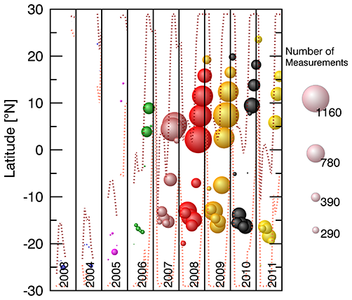
Figure 1 Number of OSIRIS mesospheric night mode scans for each month between 2003 and 2011 carried out on the ascending leg of the satellite's flight path and with an SZA >101^∘. We show one circle for each month; while the size of the circle represents the number of measurements in this months in the 30^∘ S to 30^∘ N latitude band, the position of the circle corresponds to the average latitude of the measurements in this months. The dotted lines show the minimum and maximum latitude of the available OSIRIS measurements.

Figure 1 shows the number of measurements available in every month carried out on the ascending leg of the satellites flight path and with a solar zenith angle (SZA) larger than 101^∘ during that time period and the mean latitude of the measurements. It is obvious that before 2006 only very few measurements are available and that their mean latitude is shifted to higher latitudes compared to the measurements in later years. To ensure a good comparison we have therefore decided to only include data from the time period 2006 to 2011 into this study. Lastly, to ensure only nighttime measurements are used for further analysis, we filtered the data for measurements obtained at an SZA higher than 101^∘.

Pre-processing of OSIRIS data

Several steps have to be taken to make the OSIRIS data usable for the retrieval of sodium profiles. Issues are the variable tangent height grid on which the data are measured and dark currents. With the former we deal with linear interpolation on a standard tangent height grid of 2 km and with the second we deal with offset subtraction. For detailed information see Koch et al. (2021).

Figure 2 shows the resulting spectra from a typical scan after all the necessary steps are taken before the spectra can be used to calculate limb emission rate (LER) profiles, which themselves are the first step to obtain sodium profiles.

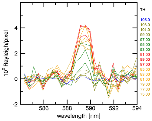
Figure 2 Monthly mean OSIRIS Na D-line nightglow spectra for April 2006 after offset and linear fit subtraction. Every colored spectrum refers to one tangent height given on the right. Tangent heights are given in kilometers. For more details about the data preprocessing method we refer to Koch et al. (2021).

2.2 SCIAMACHY on Envisat

The second data set of sodium nightglow measurements used in this study was measured with the SCIAMACHY (SCanning Imaging Absorption spectrometer for Atmospheric CHartographY) instrument (Burrows et al., 1995; Bovensmann et al., 1999). It was 1 of 10 instruments on the satellite Envisat. Envisat operated from 2002 to 2012 when the European Space Agency (ESA) lost contact to the satellite. So effectively the data cover a period of 9 whole years from 2003 to 2011. Envisat was in a polar, sun-synchronous orbit with a 10:00 descending node. The low-latitude nighttime measurements used in this study were carried out at 22:00 local solar time. The satellite completed between 14 and 15 orbits per day at an altitude of about 800 km. SCIAMACHY performed measurements in nadir, limb and occultation mode. Its eight detector channels measured electromagnetic radiation from 214 to 2384 nm, with a wavelength-dependent spectral resolution between 0.2 and 1.5 nm. The 589 nm region, which is important for this study, is covered with a spectral sampling of about 0.4 nm. In this study, only the mesosphere/lower thermosphere limb measurements on the earth's night side were used. In the limb mode the instrument scanned tangentially through the atmosphere in steps of about 3 km from 75 to 150 km tangent height and with a field of view of 110 km horizontally and about 2.6 km vertically. Additionally, we decided to only analyze monthly mean spectra with a mean signal-to-noise ratio (SNR) that is greater than 3. To obtain this value we summed up all the radiances at the sodium D-line wavelengths and divided that signal by the noise. The noise we determined to be the standard deviation of a part of the spectrum where there is no sodium D-line emission and that is equally wide as the part of the spectrum where the signal is located at. We did this for every tangent height and averaged the values.

2.3 GOMOS on Envisat

Global ozone monitoring by occultation of stars (GOMOS) on Envisat was primarily designed to monitor stratospheric ozone and other chemical species in the earth's atmosphere (Bertaux et al., 2004). While the satellite moves along its orbit, spectral radiances of several stars are recorded with 0.5 s integration time and a vertical resolution better than 1.7 km. GOMOS observed several hundred star occultations every day and it measures in both day and night conditions. The spectral ranges of the GOMOS spectrometers are 250–690, 750–776 and 916–956 nm, and careful statistical processing of the transmittance data reveals the clear spectral signature of the sodium D2–D1 doublet at 589.16 and 589.76 nm respectively (Fussen et al., 2004, 2010). The Na climatology used in this study was obtained by fitting a sodium concentration model to the GOMOS data (Fussen et al., 2010).

2.4 SABER on TIMED

To retrieve sodium profiles from measurements of the Na D-line nightglow emission, it is required to have knowledge of the corresponding ozone concentration profiles. This study was challenged by the fact that we compare measurements from instruments that measure at different local times (OSIRIS: ca. 18:50; SCIAMACHY 22:00). To make sure the obtained sodium profiles are comparable, we need ozone profiles from an instrument that provides measurements at different local times. So, we decided to use ozone profiles from the SABER (Sounding of the Atmosphere using Broadband Emission Radiometry) instrument (9.6 µm channel, data product: Level 2a, Version: 2.0) (Russell III et al., 1994). The ozone data are, like the OSIRIS and SCIAMACHY data, filtered for the −30 to 30^∘ N latitude band and for every month of the time span between 2006 and 2011. Additionally, only measurements at a solar zenith angle (SZA) higher than 101^∘ are used for further analysis. In that way, it was ensured that the sun has fully set and only nighttime measurements are considered. All the remaining measurements are sorted according to local times with a binning of 15 min. To select the ozone data that correspond to the OSIRIS and SCIAMACHY measurements, we determine the mean local solar time of all the OSIRIS measurements in 1 month, and then we average all the SABER data in a time interval ranging from that time to 30 min after the mean local time.

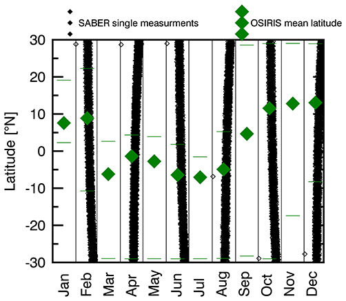
Figure 3 Collocation of the mean latitude of the OSIRIS monthly mean spectra (green diamonds) and the SABER measurements (black) that were made between 18:30 and 20:00 local time in the year 2008. The green horizontal lines indicate the maximum and minimum latitude of the OSIRIS measurements.

Using SABER data for the OSIRIS sodium retrieval showed that collocated measurements are not available in every month, between 30^∘ S and 30^∘ N latitude and at around 18:50 local time. Figure 3 shows all the single measurements of SABER in that latitude band (black) and the mean latitude of the OSIRIS measurements (green). It can be seen that measurements at that local time are only available about every second month. In summary, considering only the months in which OSIRIS measurements in the 30^∘ S to 30^∘ N latitude range with a maximum tangent height of at least 103 km and both SCIAMACHY and SABER measurements are available leaves 34 months that are suitable for comparison.

2.5 Background atmosphere from NRLMSIS-00

Finally, to determine the background atmosphere, temperature, O₂ and N₂ profiles are taken from the NRLMSIS-00 atmosphere model (Picone et al., 2002). The data were filtered for the latitude band described previously, and then we took one profile for every month at 18:00 or 22:00 for OSIRIS and SCIAMACHY, respectively.

3 Methodology

To retrieve sodium concentration profiles from volume emission rate (VER) profiles of the Na D-line nightglow at 589 nm, we used the approach first proposed by Xu et al. (2005). They showed that the Na chemistry is dominated by only three reactions. Those are Reactions (1) and (2) of the Chapman mechanism and the following additional Na loss reaction:

$$\begin{array}{}\text{(6)}& \mathrm{Na}+{\mathrm{O}}_{\mathrm{2}}+\mathrm{M}\stackrel{k_{\mathrm{3}}}{⟶}{\mathrm{NaO}}_{\mathrm{2}}+\mathrm{M}.\end{array}$$

The steady-state assumption leads to the following equation:

$$\begin{array}{}\text{(7)}& [\mathrm{Na}{]}_{\mathrm{ret}}={\displaystyle \frac{\text{VER}/f}{k_{\mathrm{1}}\left[{\mathrm{O}}_{\mathrm{3}}\right]+k_{\mathrm{3}}\left[{\mathrm{O}}_{\mathrm{2}}\right]\left[\mathrm{M}\right]}}.\end{array}$$

Xu et al. (2005) demonstrated that neglecting all other chemical reactions leads to Na retrieval errors of less than 1 %. Here, f is the effective branching ratio ($f=\mathrm{0.064}\pm \mathrm{0.024}$, taken from Koch et al., 2021), and k₁ and k₃ are reaction rate constants. For k₁ we use $\mathrm{1.1}\times {\mathrm{10}}^{-\mathrm{9}}\exp (-\mathrm{116}/T){\mathrm{cm}}^{\mathrm{3}}{\mathrm{s}}^{-\mathrm{1}}$ and for k₃ $(\mathrm{5.0}\times {\mathrm{10}}^{-\mathrm{30}})(T/\mathrm{200}{)}^{-\mathrm{1.22}}{\mathrm{cm}}^{\mathrm{6}}{\mathrm{s}}^{-\mathrm{1}}$. Both values are taken from Plane et al. (2015). For more detailed information see Koch et al. (2021) and von Savigny et al. (2016).

Retrieval approach and self-absorption correction

In this section we explain how we adjusted the method to use the OSIRIS data instead of the SCIAMACHY data.

To obtain a LER from the spectrum shown in Fig. 2 all the intensities at wavelengths between 588.3 and 591.1 nm are summed up. Possible negative non-physical values in the obtained LER profile, resulting from noise, are set to zero because the retrieval does not work with negative LER values. Negative LER values lead to negative VER values, and with those the self-absorption correction fails to give reasonable Na values. Omitting negative values of LERs may lead to a positive bias in the resulting VERs and sodium concentrations. We accept the possible positive bias, because negative LERs never occur in the peak regions but only at high altitudes. In that way, LER profiles, one for every month, are obtained. Figure 4a shows an OSIRIS LER profile for April 2004. Because the measurements are only available up to 103 km and it is assumed that the LER profiles are zero above that tangent height, we add zero values to all tangent heights up to 110 km.

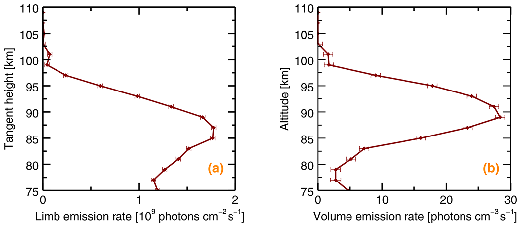
Figure 4 (a) Sample Na D-line nightglow LER profile for April 2004 determined from OSIRIS measurements. (b) Sample Na D-line nightglow VER profile that is obtained after inverting the LER profile that was obtained from OSIRIS measurements. It is assumed that there is no emission above 103 km, so the VER over 103 km is set to zero. The error bars represent the noise that is present in the spectra where no sodium signal is expected.

These LERs have to be inverted to vertical VER profiles (Fig. 4b), the first being a function of tangent height and the second being a function of the geometrical altitude. The inversion is explained in von Savigny et al. (2012) and Koch et al. (2021). The regularization parameter γ is chosen to be 1000. Additionally, the self absorption of the Na D-line emission has to be considered using the same approach as described in Langowski et al. (2016) and Koch et al. (2021).

4 Results

This study aims to compare LER, VER and sodium profiles that we have obtained from measurements with two independent (OSIRIS/Odin and SCIAMACHY/Envisat) satellite measurements. Additionally, we want to show the comparison of SCIAMACHY and OSIRIS sodium VCDs to those obtained from fitting a sodium density model to GOMOS data (Fussen et al., 2010). The comparison of the LER profiles shown in Fig. 5 of the time interval 2006 to 2011 shows that they are in good overall agreement. Here we show contour plots of SCIAMACHY (upper panel) and OSIRIS (lower panel) monthly LERs for the tangent heights between 80 and 103 km and one profile for each month. The white region in the upper panel is a result of measurements with a SNR below a certain threshold (see Sect. 2.2). The LER peaks lie between 83 and 87 km. von Savigny et al. (2016) and Unterguggenberger (2017) showed that, at low latitudes, there is a semi-annual cycle in the LERs, with peaks in the spring and fall months. Here, we see the same cycle. Looking at the VER contour plots in Fig. 6 we also see a very good agreement between the SCIAMACHY and OSIRIS VERs. The VERs are shown for altitudes between 80 and 103 km. Although there are more fluctuations than in the LERs, the VER peak is identifiable at around 91 km. Again the semi-annual cycle is clearly visible. To visualize this cycle even better we show the LERs, VERs and also sodium concentration profiles for two tangent heights/altitudes in Fig. 7. This figure shows the LERs (panels a and b) and VERs (panels c and d) at 83 and 93 km tangent height and altitude, respectively. For the sodium concentration we chose to show the altitudes of 93 and 95 km. In panels (a) and (b) the semi-annual cycle of the LERs can be seen very clearly. The panels also show that the SCIAMACHY LER peaks are slightly larger with peak magnitudes of about 2.5×10⁹ photons cm⁻² s⁻¹ than the LER peaks of OSIRIS that are only 2×10⁹ photons cm⁻² s⁻¹, i.e., 20 % lower. In Fig. 7c and d, which show the VER, we find the same semi-annual cycle as in the LERs and again SCIAMACHY shows slightly higher values than OSIRIS. While the OSIRIS peak emissions are between 20 and 30 photons cm⁻³ s⁻¹, the SCIAMACHY peak emissions lie between 35 and 40 cm⁻³ s⁻¹, i.e., around 25 % higher than those of OSIRIS. Both instruments show especially high values in the year 2011. Looking at panels (e) and (f), which show the sodium concentrations at one altitude, the semi-annual cycle is not as clearly visible. Although the reason is not fully understood we attribute it to the fact that the semi-annual oscillation of the LERs and VERs has its origin in the semi-annual oscillation of the ozone concentration. Other studies that dealt with the sodium layer in the tropics also show that seasonal variations are weaker in the tropics and stronger at high latitudes (Langowski et al., 2017; Plane et al., 2015). Since we can only retrieve OSIRIS sodium concentration profiles for every second month, we interpolated the values in between. Hereby, the green diamonds correspond to the retrieved values.

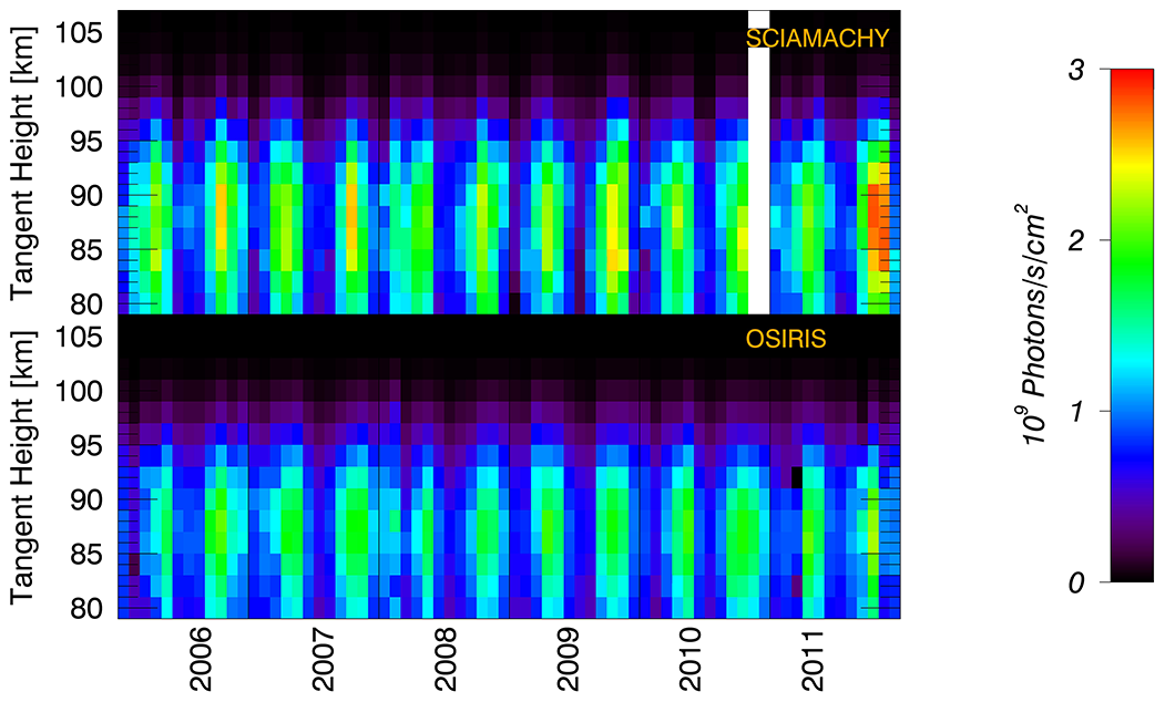
Figure 5 Time and altitude dependence of LER calculated from SCIAMACHY and OSIRIS nighttime limb measurements. We averaged over all measurements carried out in one month and in the −30 to 30^∘ latitude band. Both instruments detect a semi-annual cycle with peaks in the spring and fall months. The white regions are previously selected regions with a low SNR.

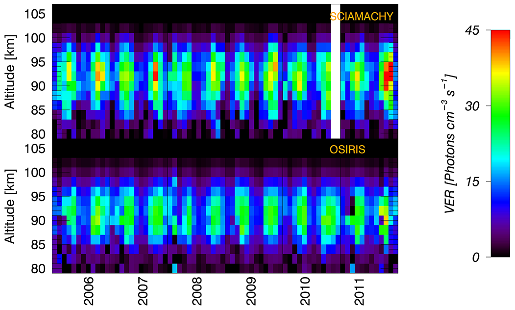
Figure 6 VER after inversion of LERs from SCIAMACHY and OSIRIS Na D-line nighttime limb measurements which are shown in shown in Fig. 5. Both instruments detect a semi-annual cycle with peaks in the spring and fall months. The white regions are previously filtered regions with a low SNR.

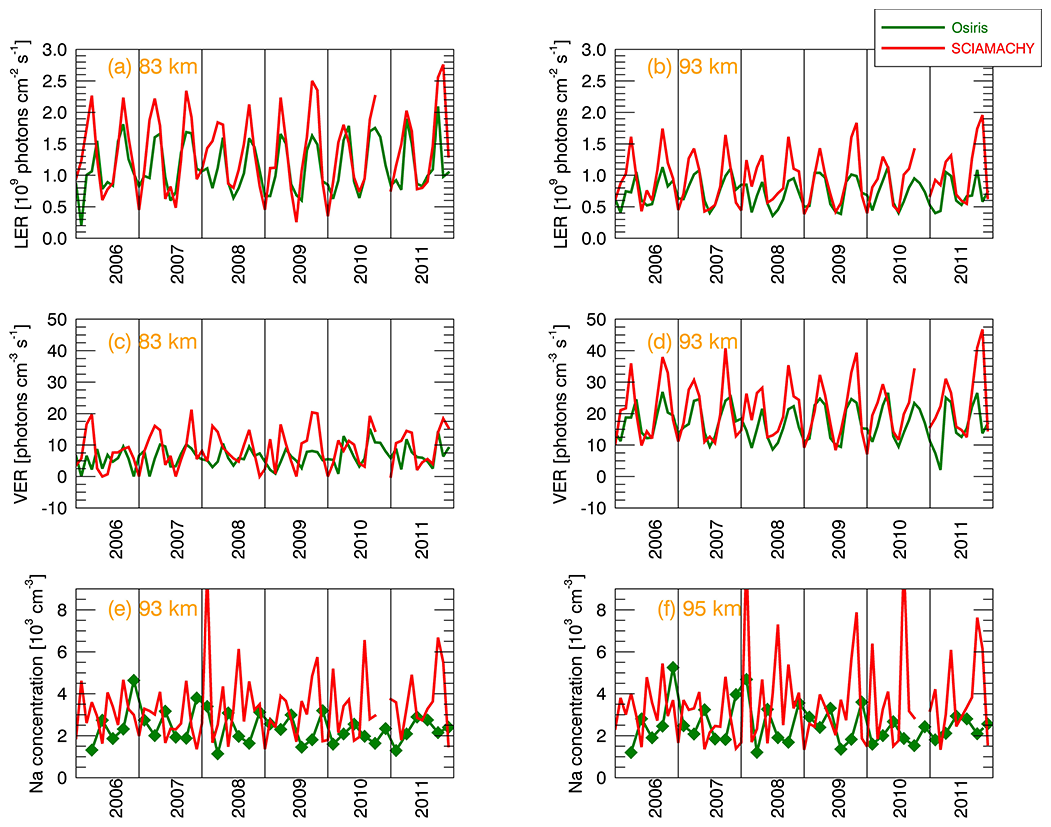
Figure 7 (a) LERs of OSIRIS and SCIAMACHY at 83 km and (b) 93 km tangent height; (c) VERs of OSIRIS and SCIAMACHY at 83 km and (d) 93 km altitude and (e) sodium concentrations of OSIRIS and SCIAMACHY at 93 km and (f) 95 km altitude. Because sodium concentrations from OSIRIS D-line nightglow measurements are only available every second month due two availability of SABER data and in order to help comparability between the two satellite measurements, we interpolated linearly between the available sodium concentrations. The actual results are marked with green diamonds, while the interpolated data points have no symbol.

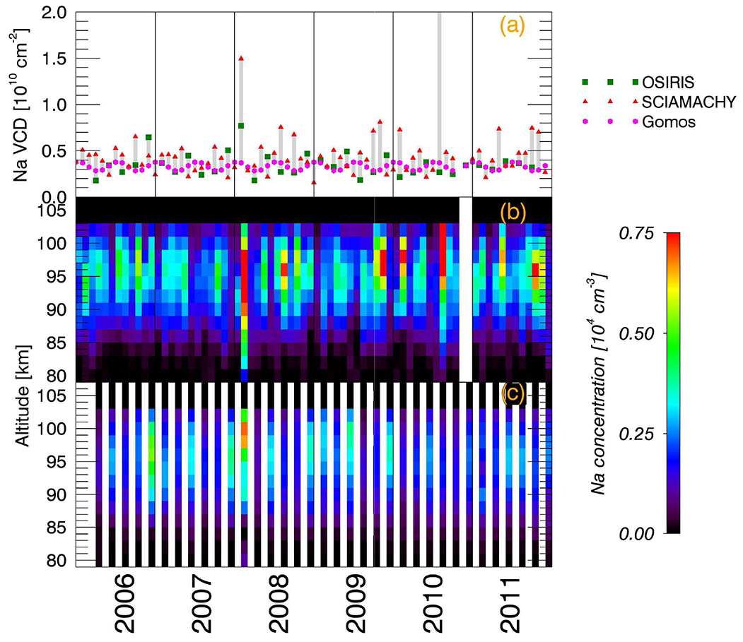
Figure 8 (a) Sodium vertical column densities obtained from OSIRIS nighttime limb measurements (green), SCIAMACHY nighttime limb measurements (red) and a sodium density model (pink) that was fitted to the GOMOS measurements (Fussen et al., 2010). (b) SCIAMACHY sodium concentration profiles. (c) OSIRIS sodium concentration profiles. All profiles and vertical columns are monthly and zonal averages.

Figure 8 shows the comparison of the sodium concentration profiles (panel b – SCIAMACHY and c – OSIRIS) as well as the VCDs (panel a). It is obvious that although the shape of the profiles can be slightly different, the values of the sodium concentrations detected by the two instruments agree well with each other. The exact reasons for the high variability, especially of the SCIAMACHY sodium profiles, are currently not fully understood. In panels (c) and (b) the sodium concentrations for the altitudes between 80 and 103 km are shown. The sodium peaks are located between 93 and 98 km and vary strongly from month to month and between the instruments. The white months in panel (c) are a result of missing co-located measurements between the SABER (ozone concentration profiles) and OSIRIS measurements. In panel (a) we show the VCDs of OSIRIS measurements (green squares), SCIAMACHY measurements (red triangles) and those obtained when fitting a sodium density model to the GOMOS data (pink circles). The latter show a very regular seasonal evolution, which is not as clearly present in the OSIRIS and SCIAMACHY VCDs. Moreover, the SCIAMACHY measurements in most months lead to higher sodium VCDs than the OSIRIS measurements. That becomes even clearer when looking at the mean values of the sodium VCDs: OSIRIS VCD $=\mathrm{3.37}\times {\mathrm{10}}^{\mathrm{9}}\pm \mathrm{1.07}\times {\mathrm{10}}^{\mathrm{9}}\mathrm{atoms}{\mathrm{cm}}^{-\mathrm{2}}$; SCIAMACHY VCD $=\mathrm{4.25}\times {\mathrm{10}}^{\mathrm{9}}\pm \mathrm{1.52}\times {\mathrm{10}}^{\mathrm{9}}\mathrm{atoms}{\mathrm{cm}}^{-\mathrm{2}}$; GOMOS VCD $=\mathrm{3.30}\times {\mathrm{10}}^{\mathrm{9}}\pm \mathrm{3.54}\times {\mathrm{10}}^{\mathrm{8}}\mathrm{atoms}{\mathrm{cm}}^{-\mathrm{2}}$. In Fig. 9 we then show the comparison of sodium profiles retrieved from OSIRIS and SCIAMACHY measurements in four different months of the year 2008 with uncertainties corresponding to each altitude. It can be seen in panels (a) and (c) that SCIAMACHY yields higher values than OSIRIS and in panel (b) the opposite is the case. Only in panel (d) the values of the sodium concentration profiles agree well with each other. We assumed the errors of N₂ and O₂ are 5 % of their concentration,; for the mesospheric temperatures we assumed an error of 10 K and for the ozone concentration we used the standard error of the mean. That we determined by dividing the standard deviation of the ozone concentrations at a certain altitude by the square root of the number of measurements which we averaged over to determine the ozone profile. For the error of the sodium nightglow emission we took the highest available tangent height and calculated the standard deviation of a part of the spectrum that has no sodium emission and the same number of pixels as the part of the spectrum with emission. We then determined the overall sodium concentration uncertainty by propagation of uncertainty. At an altitude of 95 km it lies between 2 % and 15 %. But in some months the uncertainties can go up to 25 % and above 98 km the sodium uncertainties become very large with values over 200 %. The absolute calibration uncertainty of the two instruments could also influence the retrieved sodium profiles. For OSIRIS it is estimated to lie between 5 % and 10 % while for SCIAMACHY it is between 2 % and 4 %. We tested how this could affect the sodium profiles by changing the LER profiles by ±10 %. This changes the resulting sodium profiles by around 15 %.

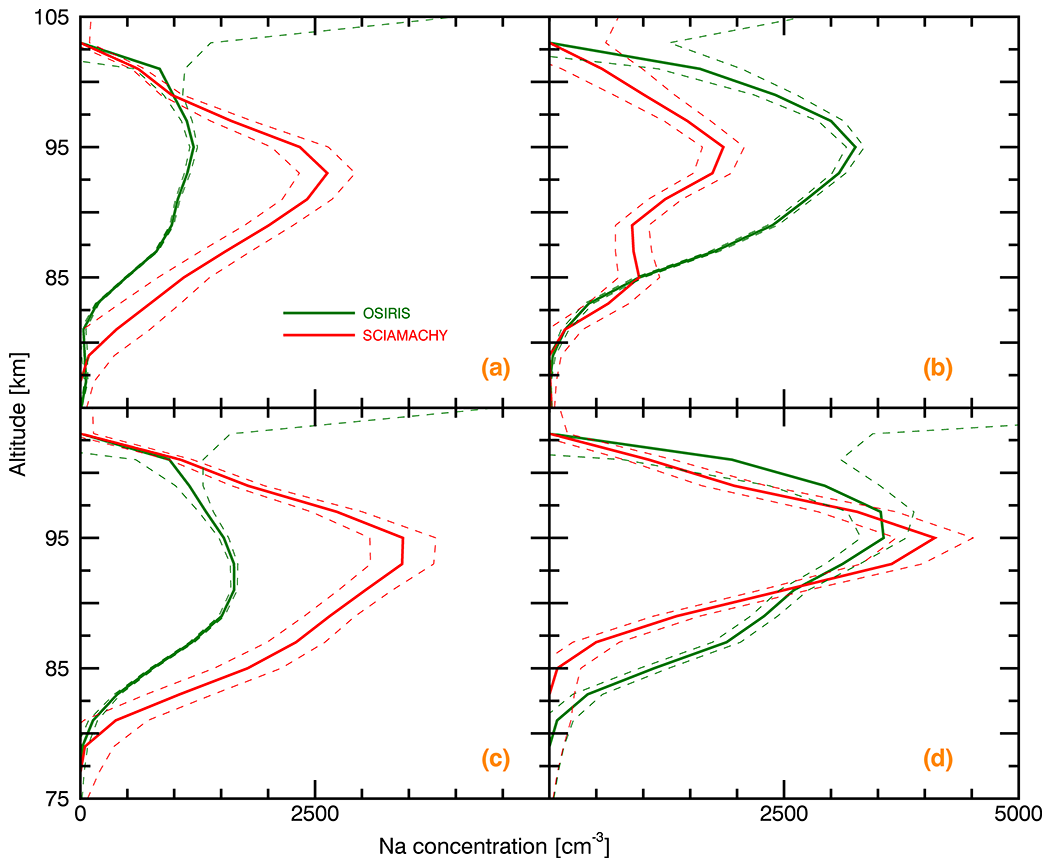
Figure 9 Sodium profiles retrieved from OSIRIS (green) and SCIAMACHY (red) mesospheric nighttime measurements for four months of the year 2008. (a) April 2008; (b) June 2008; (c) October 2008; (d) December 2008. The dashed lines show the uncertainties corresponding to each altitude.

The differences between SCIAMACHY and OSIRIS become even more obvious when looking at the mean profile of all the available profiles (Fig. 10). Here, we summed up the values of the LERs, VERs and sodium profiles at each tangent height/altitude of every available month and then divided the value by the number of months for that we could retrieve sodium concentration profiles. The mean LER, VER and sodium profiles retrieved from SCIAMACHY (red) are slightly larger than the mean profiles of OSIRIS (green). The dashed lines show the standard deviations for every corresponding tangent height/altitude. For the mean LER profiles the standard deviation is small at high tangent heights and becomes larger between 90 and 95 km. Below 90 km it stays large. This is a difference to the standard deviation of the mean VER and sodium profiles. Here the standard deviation is low above and below the peak height and only relatively high in the peak regions at around 90 and 95 km, respectively.

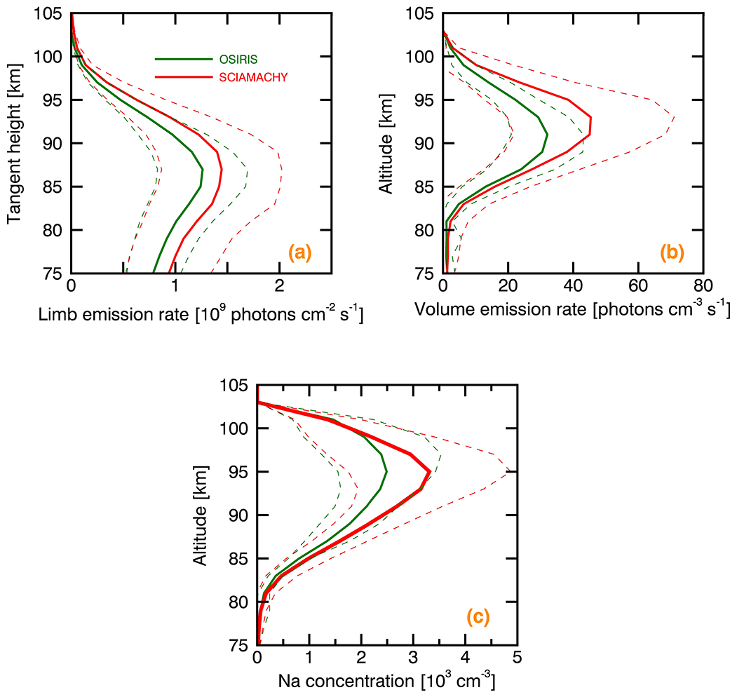
Figure 10 Comparison of mean LER profiles (a), VER profiles (b), and sodium concentration profiles (c) of SCIAMACHY (red) and OSIRIS (green) data. To obtain those profiles, we averaged over all available, i.e., 34 monthly averaged Na profiles and 67 LER profiles. The dashed lines show the standard deviation of the LER, VER and sodium concentration profiles of the corresponding altitude.

The reasons for the larger overall values of the SCIAMACHY measurements could be that OSIRIS conducts measurements with a different latitudinal and longitudinal coverage than SCIAMACHY. The first usually only conducts measurements in one hemisphere each month; the latter covers the whole −30 to 30^∘ latitude band. Although we select the profiles of the other parameters accordingly, this difference could still be the reason for the difference in the obtained sodium concentration profiles. We found out that the parameters with the largest influence are the mesospheric ozone concentration and temperature. In Fig. 11 we show how variations of the ozone concentration and mesospheric temperature influence the corresponding sodium profiles. In the left panel we increased (dashed line) and decreased (dotted line) the temperature and show how the sodium concentration changes in relation to the sodium profile obtained when using the original temperature. Here we see that changing the temperature by 10 K changes the sodium concentration by about 5 %. In the right panel we show a similar plot for the ozone concentration. Here we changed the ozone concentration by 30 %, which corresponds to 1 standard deviation, and this leads to an increase in the sodium concentration by up to 100 %. Figure 12 shows ozone concentration profiles that are used to retrieve sodium concentration profiles from SCIAMACHY (panel a) and OSIRIS (panel b) mesospheric limb nighttime measurements. The months with no data in panel (b) are a result of the differences in latitudinal and longitudinal coverage between OSIRIS and SCIAMACHY. Ozone concentrations range between 1 and 7×10⁸ cm⁻³ with a peak at 90 km. Also there is a seasonal variation with peaks in the spring and fall months and low concentrations in the northern hemispheric summer and winter. We found out that low ozone concentrations, as stated by Eq. (7), are related to high retrieved sodium concentrations, especially regarding the SCIAMACHY measurements. All ozone measurements are taken from the SABER/TIMED database. Ozone is photolyzed when the sun is present but recovers very quickly after sunset and is expected to be almost constant during the night (Vaughan, 1982; Schneider et al., 2005; Kreyling et al., 2013). The differences seen in Fig. 12 are probably mainly a result of the different latitudinal and temporal coverage of OSIRIS and SCIAMACHY. SCIAMACHY covers the whole 30^∘ S to 30^∘ N latitude band, while OSIRIS usually covers only one hemisphere and the SABER measurements are selected accordingly.

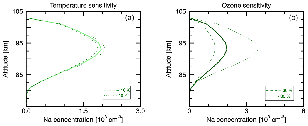
Figure 11 Sensitivity of the sodium profile to temperature changes by ±10 K (a) and ozone changes by ±30 % (b).

Figure 12 Comparison of ozone profiles from SABER measurements used to retrieve sodium concentrations from (a) SCIAMACHY and (b) OSIRIS mesospheric nighttime limb measurements.

Also the local time of the measurements could influence the sodium profiles. As OSIRIS conducts measurements around 18:50 and SCIAMACHY at 22:00, we select the ozone profiles obtained at those local times to until 30 min later and average over all profiles that fall into this time period. Although we see in Fig. 12 that the variation of ozone between the two local times is not very big, we have seen in Fig. 11 that small variations of ozone can lead to huge differences of the sodium concentration. Additionally, we tested how that non-linearity of the sodium sensitivity to variations of the ozone concentration is affected by using monthly averaged ozone profiles. To do this we retrieved sodium concentration profiles with each individual ozone profile that would be used for averaging. Then we averaged over all the resulting sodium profiles and compared this profile to the profile obtained when using one monthly averaged ozone profile. The result is, in most months, a difference of the peak sodium concentrations of around 5 %. However, in a few months the difference can be up to 20 %. In conclusion, the different latitudinal and longitudinal coverage as well as the difference of the local time of the SCIAMACHY and OSIRIS measurements together with the high variability in the mesospheric temperature and ozone profiles can have a big effect on the resulting sodium concentration profiles. And lastly, as already reported in Clemesha et al. (2011), sodium concentrations themselves are highly variable during one night. Using lidar measurements to detect the sodium layer over São José dos Campos (23^∘ S, 46^∘ W) they found variations between 2500 and 5000 atoms cm⁻³.

5 Conclusions

In this study, we compared sodium concentration profiles retrieved from Na D-line nightglow measurements from two different instruments, the Optical Spectrograph and Infrared Imager System (OSIRIS) and the Scanning Imaging Absorption Spectrometer for Atmospheric Cartography (SCIAMACHY). We were able to retrieve sodium concentration profiles with uncertainties between 2 % and 15 %, and over the period 2006 to 2011 we found 34 months that were suitable for comparison. We found out that, while SCIAMACHY detects slightly larger LERs and VERs, the overall seasonal variation of the three parameters agrees very well. To retrieve the sodium concentration we used a branching ratio of 0.064±0.024 which was determined by Koch et al. (2021). A very similar value was calculated by Unterguggenberger (2017) using ozone concentrations profiles from the SABER instrument, which is close to the value found by von Savigny et al. (2016). We were able to show that, as was expected, the LERs and VERs undergo a semi-annual cycle in the tropics. It was then concluded that the higher concentrations detected by SCIAMACHY could be primarily a consequence of the differences in the spatial and temporal coverage. While SCIAMACHY usually covers both hemispheres in the −30 to 30^∘ latitude band at 22:00 local time, the OSIRIS measurements only cover one of the hemispheres each month at around 18:50 local time. Additionally, the SCIAMACHY mesospheric nighttime limb measurements, as a result of SCIAMACHY's photodiode array, have a lower SNR than the OSIRIS measurements. We then analyzed how changing the parameters used to obtain sodium concentration profiles would affect those. We found out that the ozone concentrations have a huge influence on the value of the retrieved sodium. Changing the ozone concentration by 30 %, which corresponds to one standard deviation, changes the sodium concentration by up to 100 %. And lastly, we stated that differences in the sodium concentration could be a result of the local time difference between the measurements. While SCIAMACHY measures at a local time of 22:00, OSIRIS measurements are carried out at a local time around 18:50.