the Creative Commons Attribution 4.0 License.
the Creative Commons Attribution 4.0 License.
 | 10 Jan 2022
Quantification of CH4 emissions from waste disposal sites near the city of Madrid using ground- and space-based observations of COCCON, TROPOMI and IASI
Frank Hase
Matthias Schneider
Omaira García
Thomas Blumenstock
Tobias Borsdorff
Matthias Frey
Farahnaz Khosrawi
Alba Lorente
Carlos Alberti
Juan J. Bustos
André Butz
Virgilio Carreño
Emilio Cuevas
Roger Curcoll
Christopher J. Diekmann
Darko Dubravica
Benjamin Ertl
Carme Estruch
Sergio Fabián León-Luis
Carlos Marrero
Josep-Anton Morgui
Ramón Ramos
Christian Scharun
Carsten Schneider
Eliezer Sepúlveda
Carlos Toledano
Carlos Torres
The objective of this study is to derive methane (CH4) emissions from three landfills, which are found to be the most significant CH4 sources in the metropolitan area of Madrid in Spain. We derive CH4 emissions from the CH4 enhancements observed by spaceborne and ground-based instruments. We apply satellite-based measurements from the TROPOspheric Monitoring Instrument (TROPOMI) and the Infrared Atmospheric Sounding Interferometer (IASI) together with measurements from the ground-based COllaborative Carbon Column Observing Network (COCCON) instruments.
In 2018, a 2-week field campaign for measuring the atmospheric concentrations of greenhouse gases was performed in Madrid in the framework of Monitoring of the Greenhouse Gases Concentrations in Madrid (MEGEI-MAD) project. Five COCCON instruments were deployed at different locations around the Madrid city center, enabling the observation of total column-averaged CH4 mixing ratios (XCH4). Considering the prevalent wind regimes, we calculate the wind-assigned XCH4 anomalies for two opposite wind directions. Pronounced bipolar plumes are found when applying the method to NO2, which implies that our method of wind-assigned anomaly is suitable to estimate enhancements of trace gases at the urban level from satellite-based measurements. For quantifying the CH4 emissions, the wind-assigned plume method is applied to the TROPOMI XCH4 and to the lower tropospheric CH4 dry-air column ratio (TXCH4) of the combined TROPOMI+IASI product.
As CH4 emission strength we estimate 7.4 × 1025 ± 6.4 × 1024 molec. s−1 from the TROPOMI XCH4 data and 7.1 × 1025 ± 1.0 × 1025 molec. s−1 from the TROPOMI+IASI merged TXCH4 data. We use COCCON observations to estimate the local source strength as an independent method. COCCON observations indicate a weaker CH4 emission strength of 3.7 × 1025 molec. s−1 from a local source (the Valdemingómez waste plant) based on observations from a single day. This strength is lower than the one derived from the satellite observations, and it is a plausible result. This is because the analysis of the satellite data refers to a larger area, covering further emission sources in the study region, whereas the signal observed by COCCON is generated by a nearby local source. All emission rates estimated from the different observations are significantly larger than the emission rates provided via the official Spanish Register of Emissions and Pollutant Sources.
- Article
(11933 KB) - Full-text XML
- BibTeX
- EndNote


Methane (CH4) is the second most important anthropogenic greenhouse gas (GHG) after carbon dioxide (CO2) and contributes about 23.4 % to the radiative forcing by long-lived GHGs in the atmosphere (Etminan et al., 2016). The amount of atmospheric CH4 has increased 260 % with respect to pre-industrial levels, reaching 1877 ppb in 2019 (World Meteorological Organization, 2020). The global atmospheric CH4 emissions are approximately 40 % caused by natural sources (e.g., wetlands and termites), and about 60 % of emissions are from anthropogenic sources (Saunois et al., 2020). The anthropogenic sources of CH4 mainly originate from production and burning of fossil fuels, ruminant animals, agriculture and waste management (Bousquet et al., 2006; Chynoweth et al., 2001; Kirschke et al., 2013; Saunois et al., 2020). The waste management sector accounts for 21.5 % of the total anthropogenic CH4 emissions (Crippa et al., 2019), in which ∼ 44 % of emissions are from landfills. The global uncertainty share of landfills is about 55 % (Solazzo et al., 2021). The metropolitan cities are continuously growing due to population movements, industries, etc., and, thus, more and more cities incorporate landfills (and other potential CH4 sources) into their limits and influential areas, making landfills become one of the main CH4 sources. Since CH4 emissions from landfills can vary over several orders of magnitude due to different factors, e.g., the texture and thickness of cover soils, as well as seasonal climate, they become complex sources (Cambaliza et al., 2015). Therefore, the quantification of CH4 emission from landfills using spaceborne and ground-based observations is of importance for future climate emission scenarios and for monitoring changes in emissions.
Many studies have demonstrated the capabilities of satellite observations to estimate CH4 emissions, e.g., from oil and gas sector, including accidental leakages (e.g., Pandey et al., 2019; Varon et al., 2019; De Gouw et al., 2020; Schneising et al., 2020) and from coal mining (Varon et al., 2020). Launched in October 2017, the TROPOspheric Measuring Instrument (TROPOMI) on board the Copernicus Sentinel-5 Precursor satellite provides complete daily global coverage of CH4 with an unprecedented resolution. Compared to previous satellite instruments, TROPOMI is able to capture CH4 enhancements due to emissions on fine scales and to detect large point sources (Varon et al., 2019; De Gouw et al., 2020; Schneising et al., 2020). Satellite retrievals using thermal infrared nadir spectra as observed by IASI (Infrared Atmospheric Sounding Interferometer) or TES (Tropospheric Emission Spectrometer) are especially sensitive to CH4 concentrations between the middle troposphere and the stratosphere (e.g., Siddans et al., 2017; García et al., 2018; De Wachter et al., 2017; Kulawik et al., 2021; Schneider et al., 2021a). Schneider et al. (2021a) developed an a posteriori method for combining the TROPOMI and IASI products to detect tropospheric CH4, which has a positive bias of ∼ 1 % with respect to the reference data. The Total Carbon Column Observing Network (TCCON), a network of high-resolution Fourier-transform infrared spectroscopy (FTIR) spectrometers (Washenfelder et al., 2006), has been designed to provide accurate and long-lasting time series of column-averaged dry-air molar fractions of GHGs and other atmospheric constituents (Wunch et al., 2011). Recently, TCCON GHG observations have been extended by the COllaborative Carbon Column Observing Network (COCCON, Frey et al., 2019), which is a research infrastructure using well-calibrated low-resolution FTIR spectrometers (Bruker EM27/SUN, Gisi et al., 2012) and a common data analysis scheme. Due to the ruggedness of the portable devices used and simple operability, COCCON is well suited for implementing arrays of spectrometers in metropolitan areas for the quantification of local GHG sources (Hase et al., 2015; Luther et al., 2019; Vogel et al., 2019; Dietrich et al., 2021).
Madrid, Spain, is one of the biggest cities in Europe and has almost 3.3 million inhabitants, with a metropolitan area population of approximately 6.5 million. Thus, the waste is one of the main CH4 emission sources. To measure atmospheric concentrations of GHGs in this urban environment, a 2-week campaign was carried out in the framework of the Monitoring of the Greenhouse Gases Concentrations in Madrid (MEGEI-MAD) project (García et al., 2019) from 24 September to 7 October 2018 in Madrid.
In this study we analyze nearly 3 years of TROPOMI total column-averaged dry-air molar fraction of CH4 (XCH4) measurements, TROPOMI+IASI TXCH4 measurements together with COCCON spectrometer observations made during the MEGEI-MAD campaign, in an attempt to quantify the CH4 emissions from major emission sources – namely three landfills in Madrid, the most important metropolitan area of Spain. In Sect. 2 our methodology is described, which is as follows: we calculate the difference of the satellite data maps for two opposite wind regimes (we refer to the resulting signals as wind-assigned anomalies). A simple plume model is then applied to predict the wind-assigned anomalies for a chosen position and strength of a source. The results of our study are presented and discussed in Sect. 3, and the conclusions from these results are given in Sect. 4.
2.1 Ground-based and spaceborne instrumentations
2.1.1 COCCON XCH4 data set
The Bruker EM27/SUN is a robust and portable FTIR spectrometer, operating at a medium spectral resolution of 0.5 cm−1. The EM27/SUN FTIR spectrometer has been developed by the Karlsruhe Institute of Technology (KIT) in cooperation with Bruker Optics GmbH for measuring GHG concentrations (Gisi et al., 2012; Hase et al., 2016). An InGaAs (indium gallium arsenide) photodetector is used as the primary detector, covering a spectral range of 5500–11 000 cm−1. A decoupling mirror reflects 40 % of the incoming converging beam to an extended InGaAs photodetector element, covering the spectral range of 4000–5500 cm−1 for simultaneous carbon monoxide (CO) observations. The recording time, for a typical measurement consisting of five forward and five backward scans, is about 58 s in total.
Several successful field campaigns and long-term deployments have demonstrated that the Bruker EM27/SUN FTIR spectrometer is an excellent instrument with good quality, robustness and reliability, and its performance offers the potential to support TCCON (Frey et al., 2015, 2019; Klappenbach et al., 2015; Chen et al., 2016; Butz et al., 2017; Sha et al., 2020; Jacobs et al., 2020; Tu et al., 2020a, b; Dietrich et al., 2021). The Bruker EM27/SUN spectrometers have become commercially available from April 2014 onwards, and currently about 70 spectrometers are operated by different working groups in Germany, France, Spain, Finland, Romania, USA, Canada, UK, India, Korea, Botswana, Japan, China, Mexico, Brazil, Australia and New Zealand. The development of the COCCON (https://www.imk-asf.kit.edu/english/COCCON.php, last access: 22 December 2020) became possible by continued European Space Agency (ESA) support. COCCON intends to become a supporting infrastructure for GHG measurements based on common standards and data analysis procedures for the EM27/SUN (Frey et al., 2019).
All the Bruker EM27/SUN spectrometers used in the MEGEI-MAD project were operated in accordance with COCCON requirements. The resulting XCH4 data used in this work were generated by the central facility operated by KIT for demonstrating a centralized data retrieval for the COCCON network. For these reasons, we refer to the Bruker EM27/SUN spectrometers as COCCON spectrometers in the following. The COCCON XCH4 data product is derived from the co-observed total column amounts of CH4 and oxygen (O2), and the assumed dry-air molar fraction of O2 (0.2095) (Wunch et al., 2015):
2.1.2 TROPOMI XCH4 data set
The TROPOMI data processing deploys the RemoTeC algorithm (Butz et al., 2009, 2011; Hasekamp and Butz, 2008) to retrieve XCH4 from TROPOMI measurements of sunlight backscattered by the Earth's surface and atmosphere in the near-infrared (NIR) and shortwave-infrared (SWIR) spectral bands (Hu et al., 2016, 2018; Hasekamp et al., 2021; Landgraf et al., 2019). This algorithm has been extensively used to derive CH4 and CO2 from GOSAT (Butz et al., 2011; Guerlet et al., 2013). The TROPOMI XCH4 is calculated from the CH4 vertical sub-columns xi and the dry-air column. The dry-air column is obtained from the surface pressure from the European Centre for Medium-Range Weather Forecasts (ECMWF) and from the altitude from the Shuttle Radar Topography Mission (SRTM) (Farr et al., 2007) digital elevation map with a resolution of 15 arcsec (Lorente et al., 2021a):
This study uses the TROPOMI data set of XCH4 from Lorente et al. (2021a), for which an updated retrieval algorithm was implemented to obtain a data set with less scatter. This updated XCH4 has been demonstrated to be in good agreement with TCCON (−3.4 ± 5.6 ppb) and GOSAT ( ppb), with a bias and precision below 1 %. Here the TROPOMI XCH4 between 30 April 2018 and 30 December 2020 within the rectangular area of 39.5–41.5∘ N and 4.5–3.0∘ W (125 km × 220 km) over Madrid is analyzed. In addition, we apply strict quality control to TROPOMI XCH4 (quality value q=1.0) to exclude data of questionable quality and to assure data under clear-sky and low-cloud atmospheric conditions (Lorente et al., 2021a).
2.1.3 IASI CH4 data and their synergetic combination with TROPOMI data
The IASI sensors are currently orbiting aboard three Metop (Meteorological Operational) satellites and offer global coverage twice daily with high horizontal resolution (ground pixel diameter at nadir is 12 km). The IASI CH4 products have a particular good quality and sensitivity as documented in validation studies (e.g., Siddans et al., 2017; De Wachter et al., 2017; García et al., 2018; Schneider et al., 2021a).
Here we use the IASI CH4 product as generated by the latest MUSICA IASI processor version (Schneider et al., 2021b). Combining these IASI profile data with the TROPOMI total column data causes strong synergies. Schneider et al. (2021a) developed an a posteriori method for such a synergetic combination and documented the possibility to detect tropospheric partial column-averaged dry-air molar fractions of CH4 (TXCH4) independently from the upper tropospheric/stratospheric dry-air molar fractions of CH4 (UTSXCH4). This is not possible by either the TROPOMI or IASI product individually. In this study we use a tropospheric product averaged from ground to 7 km a.s.l. and an upper tropospheric/stratospheric product averaged from 7 to 20 km a.s.l.
2.2 COCCON Madrid campaign
Madrid is located on the Meseta Central and 60 km south of the Guadarrama mountains with a considerable altitude difference across the city, ranging from 570 to 700 m a.s.l.
This work was made in the framework of the MEGEI-MAD project (García et al., 2019), which aimed to measure atmospheric concentrations of GHGs in an urban environment combining FTIR instruments and ground-level analyzers. Another objective of MEGEI-MAD was to analyze the possible use of portable COCCON instruments to shape an operational network for Madrid in the future. The MEGEI-MAD project was initiated by the Izaña Atmospheric Research Center (AEMet), in cooperation with two German research groups (the Karlsruhe Institute of Technology and the University of Heidelberg) and two Spanish research groups (the Autonomous University of Barcelona and the University of Valladolid).
Within MEGEI-MAD, a 2-week field campaign was carried out from 24 September to 7 October 2018 in Madrid, where five COCCON instruments were located at five different places circling the metropolitan area (see Fig. 1). Table 1 summarizes the coordinates, altitudes of the COCCON locations and auxiliary meteorological data collected for data analysis of the observations. The locations have been chosen by considering the prevailing winds and the emission sources of CO2 and CH4, as well as other technical and logistic criteria (García et al., 2019, 2021).
Table 1Locations of the five COCCON instruments and meteorological records for the MEGEI-MAD field campaign during 24 September–7 October 2018.
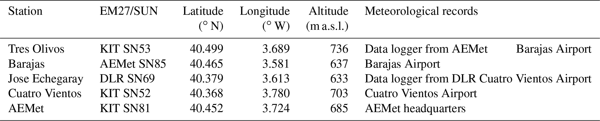
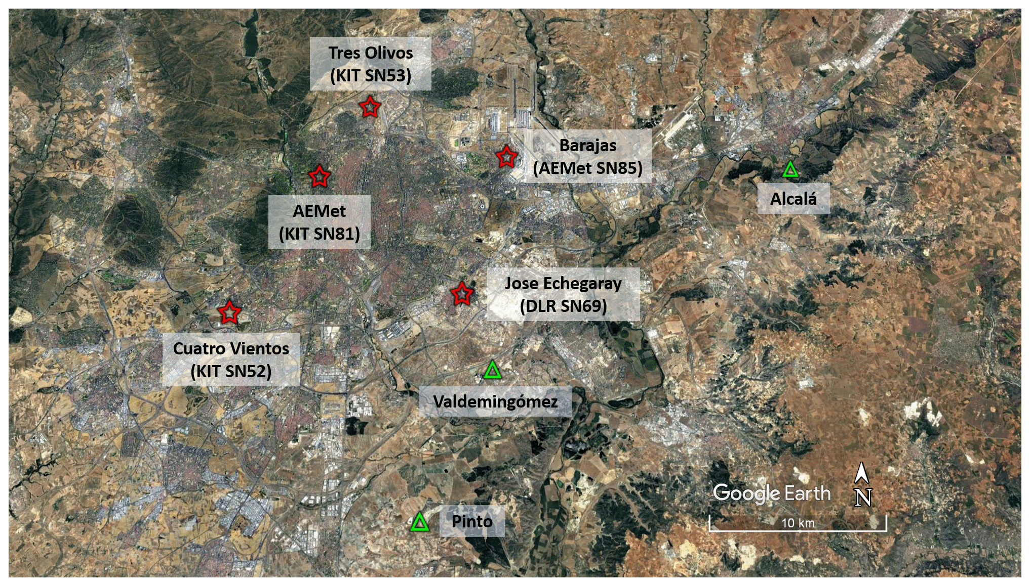
Figure 1Locations of the five COCCON instruments used in the Madrid field campaign during 24 September–7 October 2018, represented with red stars, and locations of three waste treatment and disposal plants, represented with the green triangles (image © Google Earth).
2.3 Emission strength calculation using a simple plume model
The daily plume is modeled as a function of wind direction and wind speed. The schematic dispersion model for describing emissions assumes an expanding cone-shaped plume with the tip at the plume source at location (0,0). The plume cone has an opening angle of size α, and any grid cell within the cone is affected by the emission (see Fig. 2). The angle α is a technical parameter to schematically describe a spreading of the plume and is empirically adjusted to a value of 60∘. Different opening angles are modeled and presented in Fig. A1. The modeled plume has the most similar shape compared to the TROPOMI measured NO2 plume (see Sect. 3.3) when . If the grid cell (x,y) locates inside the cone, the column enhancement for this cell can be calculated by
where ε is the emission strength at the source point in molec. s−1, v is the wind speed in m s−1, d is the distance between the downwind point and the source, and α is the opening angle of the plume in rad (here assumed to be 60∘).
The distance from a general grid cell (x,y) from the source is
The enhanced dry-air volume mixing ratio for target species (ΔXVMR) at the center of the grid cell (x,y) can then be calculated by dividing the column enhancement by the total column of dry air (columndryair):
The columndryair is computed from the surface pressure:
where Ps is the surface pressure, mdryair and are the molecular masses of dry air (∼28.96 g mol−1) and water vapor (∼18 g mol−1), respectively, columndryair and column are the total column amount of dry air and water vapor, and g(φ) is the latitude-dependent surface acceleration due to gravity.
In this study, each individual landfill is considered an individual point source. The daily plumes from the individual landfills are super-positioned to have a total daily plume. The averaged enhancement of XVMR (plume) over the study area is computed for the selected wind sector. The plume for the opposite wind regime is also constructed in the same manner. The differences between these two data sets are therefore the wind-assigned anomalies (see Sect. 3.3). By fitting the modeled wind-assigned anomalies to the anomalies as observed by the satellite, we can estimate the actual emission strength (see Sect. B2). Note that the applied calculation scheme would also be extendible to areal sources by superimposing such calculations using different locations of the origin.
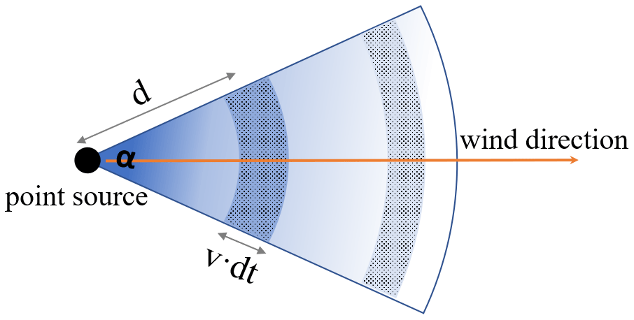
Figure 2Sketch of the simple plume model used to explain the CH4 emission estimation method. The methane at the point source is distributed along the wind direction (wind speed: v) in the cone-shaped area with an opening angle of α. The point source emits the methane at an emission rate of ε. We assumed the methane molecules are evenly distributed in the dotted area A, and the distance from area A to the point source is d. Therefore, the emitted methane in dt time period equals the amount of methane in the area A. It yields the equation .
3.1 Intercomparison of TROPOMI and COCCON XCH4 measurements
To detect whether TROPOMI is capable of measuring XCH4 precisely in the Madrid area, we perform intercomparison between TROPOMI and COCCON XCH4 measurements. Figure 3 shows the correlation between COCCON and TROPOMI measurements. The mean value of TROPOMI XCH4 is calculated by collecting observations within a radius of 5 km around each COCCON station. The coincident COCCON mean XCH4 is calculated from the measurements within 30 min before or after the TROPOMI overpass. The distance between two stations ranges between 6 and 14.2 km. The TROPOMI data within a circle with a larger radius might cover the information from other nearby stations, which brings an error in the correlation between the coincident data. Therefore, we choose a collection circle with a radius of 5 km for TROPOMI. The coincident data at each station show generally good agreement. Note that there are 1 to 2 TROPOMI measurements located within a circle of 5 km radius around each station. The mean bias in XCH4 between TROPOMI and COCCON is 2.7 ± 13.2 ppb, which is below the absolute bias between TROPOMI and TCCON (3.4 ± 5.6 ppb, Lorente et al., 2021a). The higher scatter of the validation with COCCON reflects the shorter temporal and spatial collocation, but the agreement indicates that TROPOMI data have good quality and a low bias.
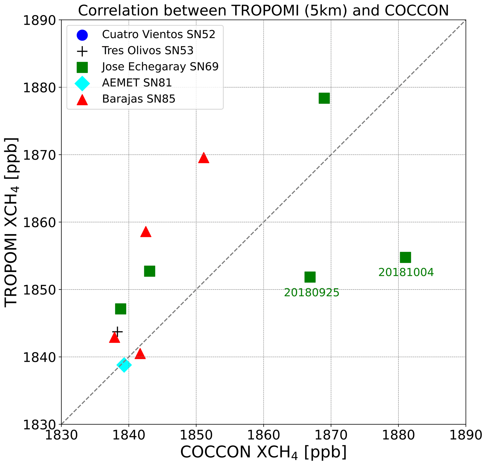
Figure 3Correlation plot between TROPOMI observations collected within 5 km radius around each COCCON station and coincident COCCON measurements (30 min before and after the TROPOMI overpass) at five stations in 2018.
The coincident data on 25 September 2018 and 4 October 2018 show large biases at Jose Echegaray station where the SN69 COCCON instrument is located. Due to its coarser spatial resolution, the TROPOMI XCH4 observations do not capture the local enhancements detected by the COCCON instrument in the vicinity of the source. Figure 4 illustrates the 2 example days of the time series of COCCON SN69 and coincident TROPOMI observations. Obvious enhancements are observed at around 13:00 UTC by the COCCON instrument in the downwind site on 25 September and at around 12:30 on 4 October 2018 (see Fig. A2 for the other days). Note that the XCH4 enhancements can also be observed by the instruments at other stations when the CH4 plume passes over Madrid. We only discuss the 2 representative days with obvious enhancements here, as we focus on the specific source near the Jose Echegaray station. The Valdemingómez and Pinto waste plants are located nearby, with a distance of 4.5 and 12 km, respectively. These five COCCON stations can serve as an independent source of information for constraining the wind speed. For example, the distance between the Jose Echegaray and Barajas is about 10 km. The highest anomalies of XCH4 arrived around 1.5 h later at Barajas station than they appeared at the Jose Echegaray station on 25 September 2018, which indicates an averaged wind speed of 1.8 m s−1. This value fits well with the wind velocity observed at the Cuatro Vientos Airport.
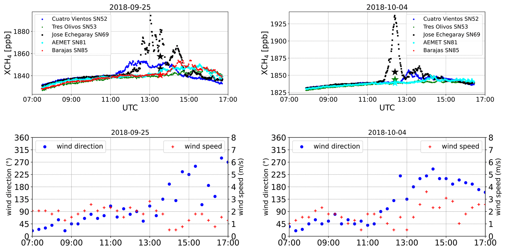
Figure 4Time series of COCCON measurements at five stations on 2 d in 2018. Star symbols represent the averaged TROPOMI observations within a radius of 5 km around each station. Lower panels show the wind direction and wind speed measured at the Cuatro Vientos Airport.
TROPOMI detected 10 ppb higher XCH4 at Jose Echegaray station than at Barajas station on 25 September 2018. However, COCCON observed a much higher amount of XCH4 (53 ppb) at Jose Echegaray station than at Barajas station (and other stations) at around 13:00 UTC. The delayed enhancements at AEMet and Barajas stations at the downwind direction are found after the wind direction changed from north more towards south direction. Another obvious enhancement of XCH4 is observed at Jose Echegaray station by the COCCON SN69 instrument at around 12:30 on 4 October 2018, with about 97 ppb higher XCH4 than COCCON measurements at the other four stations. However, TROPOMI only measured about 13 ppb higher XCH4 at Jose Echegaray station compared to the TROPOMI measurements at the other stations. These considerable enhancements at Jose Echegaray station observed by the COCCON instrument are likely due to the local source (the nearby Valdemingómez waste plant). The plume is in close vicinity to the source narrower than the pixel scale of the satellite, and therefore it is only detected as an attenuated signal by TROPOMI. The full width at the half maximum (FWHM) of the enhancement peak on 4 October 2018 roughly covers a temporal window of 30 min, with a corresponding wind direction change of 22.5∘ (∼ 0.4 rad) and an averaged wind speed of 1.0 m s−1. The distance between the COCCON SN69 to the Valdemingómez waste plant is about 4500 m. The 97 ppb enhancement measured by COCCON SN69 instrument yields an estimated emission strength of 3.7 × 1025 molec. s−1.
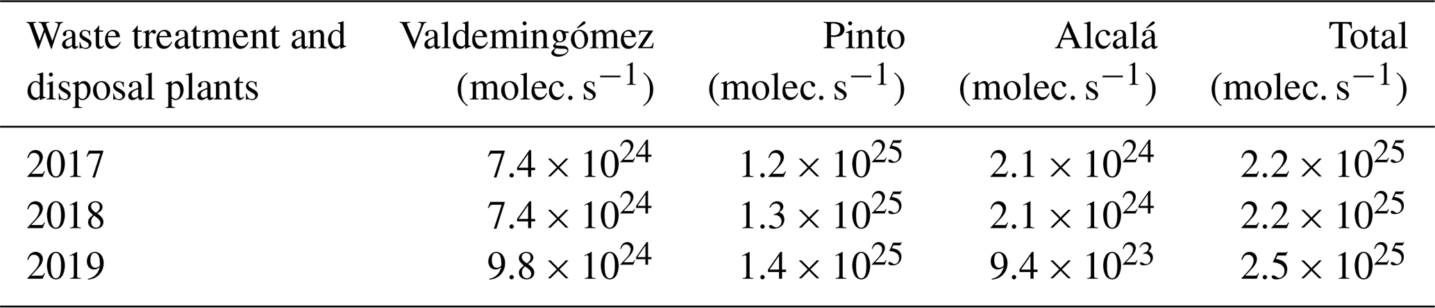
According to the Spanish Register of Emissions and Pollutant Sources (PRTR, http://www.en.prtr-es.es/, last access: 20 February 2021), more than 95 % of total CH4 emissions are from three waste treatment and disposal plants in the Madrid region (locations showed in Fig. 1). The annual CH4 emission rates from the PRTR for each plant are listed in Table 2. The total emission strength for each plant is about 2.5 × 1025 molec. s−1. This value only considers the “cells” in production, i.e., those where the waste is not yet covered with soil. The emissions from sealed cells are not included in the total emissions, but they still emit CH4 for years after sealing. So, the estimated emission rates from the inventories are expected to underestimate the true emissions, which fits reasonably with the estimated emission rate derived from COCCON measurements. The COCCON instruments show a very good ability to detect the source. Based on this evidence we investigate the potential of the TROPOMI and IASI CH4 products for detecting CH4 sources in the following.
Table 2CH4 emission rates in three waste treatment and disposal plants in Madrid from PRTR.
3.2 Predominant wind
To better represent the whole area of Madrid, the hourly ERA5 model wind at a height of 10 m around Madrid is used. ERA5 is the fifth-generation climate reanalysis produced by the European Centre for Medium-Range Weather Forecasts (ECMWF) (Copernicus Climate Change Service, 2017). The TROPOMI overpasses over Madrid cover the time range from 12:00–14:30 UTC (IASI overpasses are typically from 09:30–10:30 UTC), but the dispersion of emitted CH4 is influenced by the ground conditions (e.g., wind speed and wind direction) over a wider time range (Delkash et al., 2016; Rachor et al., 2013). Therefore, the wind information between daytime (08:00–18:00 UTC) is chosen to define the predominant wind direction for each day. Figure 5 presents the wind roses for daytime between 10 November 2017 and 10 October 2020 (the first and last day with valid TROPOMI data). The dominating wind direction was southwesterly. The Guadarrama mountains and the Jarama and Manzanares river basins are located the northwest of Madrid, and they influence the air flow. Therefore, we use a wider wind range for the specific wind area in this study to cover the dominant wind directions, i.e., SW for the range of 135–315∘ and NE for the remaining direction. If a wind direction dominates 60 % of records for 1 d, i.e., if the wind direction belongs to one specific area more than 60 % of the daytime (08:00–19:00 UTC), then this predominant wind direction is selected for that day. The SW and NE wind fields are used for constructing wind-assigned anomalies in this study, and we demonstrate this construction by using TROPOMI nitrogen dioxide (NO2) data in the next section. Table 3 summarizes the number of days and wind speed for each specific wind area. The wind direction during the TROPOMI overpasses was 61.8 % in the SW wind field and 28.4 % in the NE wind field, and their averaged wind speed is similar.
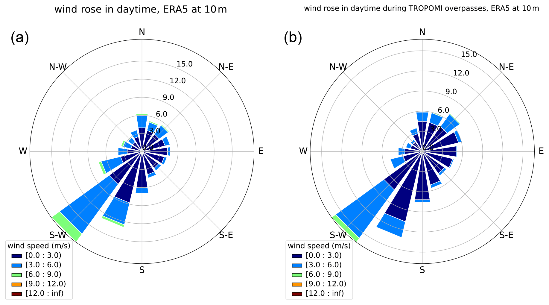
Figure 5Wind roses for daytime (08:00–19:00 UTC) from 10 November 2017 to 10 October 2020 for the ERA5 model wind. Panel (a) covers all days and panel (b) covers the days with TROPOMI overpasses.
Table 3Number of days and the averaged ERA5 wind speed (± standard deviation) per specific wind area in daytime (08:00–18:00 UTC) from 10 November 2017 to 10 October 2020. Columns 2 and 3 are for all days, and columns 4 and 5 are for days with TROPOMI overpass.

3.3 Demonstration of the wind-assigned anomaly method
When fossil fuels are burned, nitrogen monoxide (NO) is formed and emitted into the atmosphere. NO reacts with O2 to form NO2 and with ozone (O3) to produce O2 and NO2. NO2 is an extremely reactive gas with a short lifetime of a couple of hours and has lower background levels than CH4 (Kenagy et al., 2018; Shah et al., 2020). It is measured by TROPOMI with excellent quality. Therefore, it is a suitable proxy for demonstrating the method developed for the wind-assigned anomaly.
TROPOMI offers simultaneous observations of NO2 columns. The recommended quality filter value for the analysis of TROPOMI NO2 columns is qa_value > 0.75 (http://www.tropomi.eu/sites/default/files/files/publicSentinel-5P-Level-2-Product-User-Manual-Nitrogen-Dioxide.pdf, last access: 11 November 2021). Based on the predominant wind direction in Madrid (see Sect. 3.2), the averaged wind-assigned anomalies are defined here as the difference of the mean TROPOMI NO2 column under the wind direction from NE and the mean TROPOMI NO2 column under the predominant wind direction of SW in Madrid.
Figure 6a illustrates the wind-assigned anomalies of TROPOMI NO2 (ΔNO2) on a 0.1∘ × 0.135∘ latitude–longitude grid during 2018–2019. Pronounced fusiform-shaped plumes are observed along NE–SW wind direction as expected. Figure 6b shows the wind-assigned anomalies derived from the simple model introduced in Sect. 2.3, using Madrid city center as the point source with an assumed emission rate (ε) of 5.0 × 1024 molec. s−1 and using ERA5 10 m wind data. The similar symmetrical positive and negative plumes to those in Fig. 6a imply that our method of wind-assigned anomaly is working as anticipated, that the ERA5 10 m data are indeed representative for the area and that the implementation of the satellite data analysis is correct. Figure 6c shows the strong correlation between the wind-assigned anomalies derived from the TROPOMI measurements and the simple plume model (ε=5.0 × 1024 molec. s−1). Using the fitting method as described in Sect. B2, we estimate an emission rate of 3.5 × 1024 molec. s−1 ± 3.9 × 10²² molec. s−1. Here the uncertainty is due to the noise of the observations and is calculated according to Eq. (B15) (Appendix B). This estimated source strength is weaker than the strength obtained by Beirle et al. (2011), where the reported NOx emission is around 150 mol s−1 in Madrid, corresponding to a NO2 emission of 6.8 × 1025 molec. s−1. It is because our model does not consider the decay of NO2, which results in a lower emission rate.
The result of this test using NO2 also allows the angular spread parameter used in the plume model to be adjusted (see Sect. 2.3 and Eq. 3). As it can be seen from Fig. A1, assuming an angular spread of 60∘ reasonably reproduces the shape of the plume.
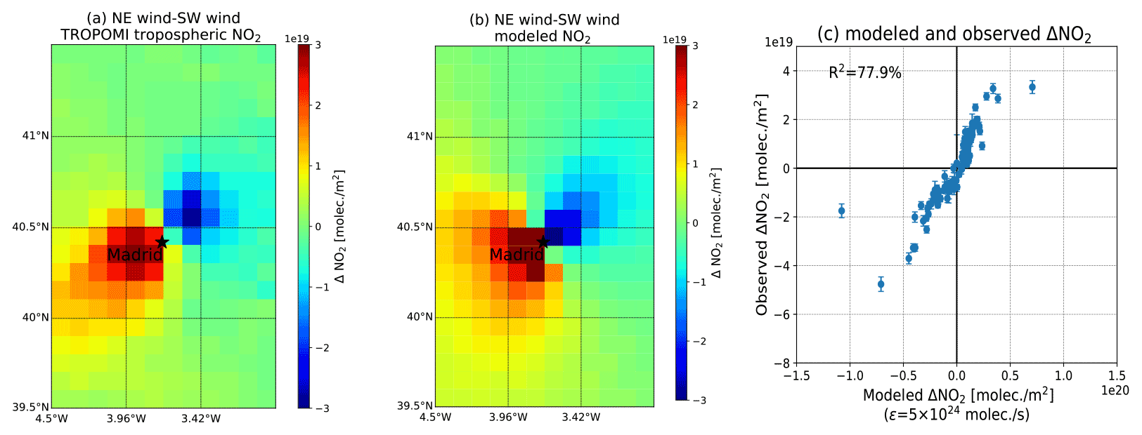
Figure 6Wind-assigned anomalies derived from (a) TROPOMI tropospheric NO2 column, (b) our simple plume model (ε=5 × 1024 molec. s−1) over Madrid in the NE–SW direction on a 0.1∘ × 0.135∘ latitude–longitude grid during 2018–2020, and (c) the correlation plot between observed ΔNO2 and modeled ΔNO2 (ε=5 × 1024 molec. s−1) during 2018–2019.
3.4 XCH4 and TXCH4 anomaly
CH4 has a relatively longer lifetime as compared to NO2, and its background in the atmosphere is high. An increasing trend with obvious seasonality and strong day-to-day signals for XCH4 is seen in Fig. 7 (upper panels). Therefore, these background signals need to be removed before simulating the wind-assigned anomalies (see Sect. B1). After removing the background, the anomalies (raw data – background) represent more or less the emission from local area (Fig. 7 lower panels).
Figure 8 illustrates the anomalies of XCH4, TXCH4 and UTSXCH4 for all measurement days, days with predominating SW wind field and days with predominating NE wind field. The distributions over the whole area for XCH4 and TXCH4 are similar, and no obvious enhancement is observed in UTSXCH4, as expected, since CH4 abundances dominate in the troposphere. The areas where the three waste plants are located show obvious high anomalies in the figures (Fig. 8a and d) when the data are averaged over all days for all wind directions and in the downwind direction (Fig. 8b, c, e and f), demonstrating that our method of removing the background works well and the satellite products can detect the local pollution sources after removing the background. Enhanced plumes of XCH4 and TXCH4 are better visible on the downwind side of SW than on the downwind side of NE wind field. This is because the SW is the most dominant wind direction, and the SW plume signal is based on a higher number of data and thus less noise.
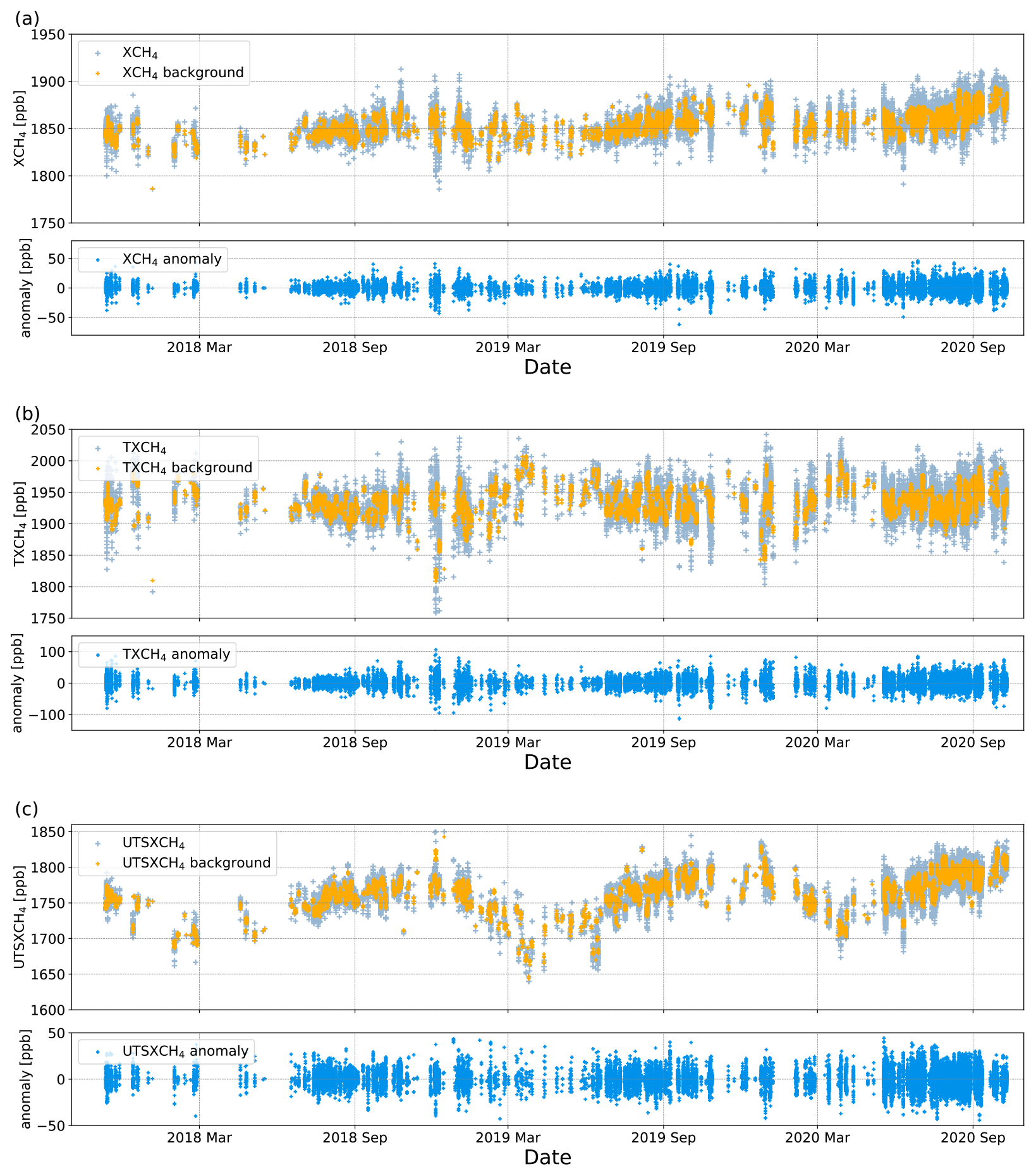
Figure 7Time series of (a) XCH4, (b) TXCH4 and (c) UTSXCH4, showing raw data and background in each upper panel and anomalies in each corresponding lower panel.
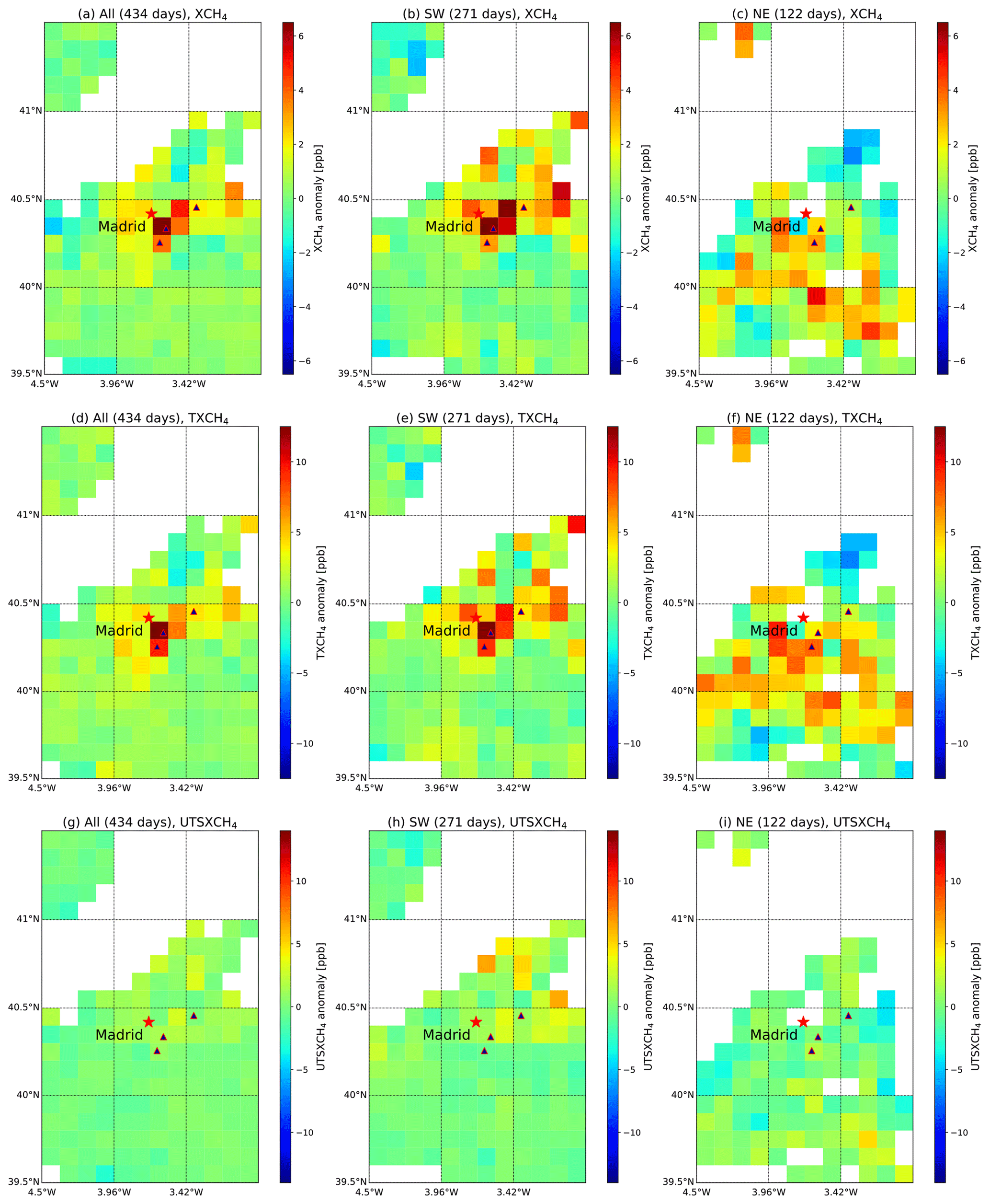
Figure 8(a–c) XCH4, (d–f) TXCH4 and (g–i) UTSXCH4 anomalies averaged for all days, days with SW wind and NE wind directions. The triangle symbols represent the location of waste plants.
3.5 Estimation of CH4 emission strengths from satellite data sets
The wind-assigned anomalies derived from XCH4 anomalies and TXCH4 anomalies on a 0.1∘ × 0.135∘ latitude–longitude grid are presented in Fig. 9. The XCH4 and TXCH4 wind-assigned anomalies show similar bipolar plumes but are more disturbed compared to those derived from NO2. This is because the CH4 signal is weak compared to the background concentration, so the noise level of the measurement and the imperfect elimination of the background are significant disturbing factors.
Based on the knowledge of the locations of the three waste plants, we choose their locations as point sources to model the enhanced XCH4 according to the wind information. The initial emission strength is 1 × 1026 molec. s−1 in total, and the emission rate at each point source is repartitioned among these three sites according to Table 2. The modeled and observed wind-assigned anomalies show a reasonable linear correlation (coefficient of determination R2 of about 49 % and 44 % for XCH4 and TXCH4, respectively) with observed ΔXCH4. Based on Eq. (B12) (Appendix B), we obtained an estimated emission rate of 7.4 × 1025 ± 6.4 × 1024 molec. s−1 for XCH4 and 7.1 × 1025 ± 1.0 × 1025 molec. s−1 for TXCH4. The uncertainty values given here are the square root sum of the uncertainty due to the background signal and the data noise, which are calculated according to Eqs. (B14) and (B15) (Appendix B). Figure 9g, h and i show the wind-assigned anomalies for UTSXCH4. For the modeled UTSXCH4 anomalies we assume here the CH4 enhancement to occur at altitudes between 7 and 20 km a.s.l. As expected, the fit of these model data to the observed UTSXCH4 data yields emission rates close to zero (1.4 × 1025 ± 7.2 × 1024 molec. s−1), revealing that there is no significant plume signal above 7 km a.s.l. The fact that for TXCH4 we obtain practically the same emission rates as for XCH4 and that in the UTSXCH4 data we see almost no plume nicely proves the quality of our careful background treatment method and the low level of cross sensitivity between the TXCH4 and UTSXCH4 data products. The applied background treatment allows detecting the near-surface emission signal consistently in the total column XCH4 data and in the tropospheric TXCH4 data.
Figure 10 illustrates the estimated emission strengths for the different products. The emission strengths derived from the satellites are higher than the ones derived from COCCON measurements, as TROPOMI covers a larger area, while COCCON measurements are only sensitive to local sources from the nearby waste plant. The PRTR inventory document gives lower values than our results. This is probably because it only lists the active landfill cells and does not include the closed ones in Madrid, which probably still emit for many years (Sánchez et al., 2019).

Figure 9Wind-assigned XCH4 plume derived from (a) TROPOMI XCH4 anomalies, (d) synergetic TXCH4 anomalies, and (g) UTSXCH4 anomalies and their corresponding modeled plume (b, e, h) over Madrid in the NE–SW direction on a 0.1∘ × 0.135∘ latitude–longitude grid. The correlation plots between observed ΔXCH4 and modeled ΔXCH4 (ε=1 × 1026 molec. s−1) for different products (c, f, i). Here we use the three waste plants as the point sources (blue triangle with red edge color). The initial emission rate in the plume model is 1 × 1026 molec. s−1. This value is proportionally distributed into three point sources based on the a priori knowledge of emission rate in each waste plant. For the modeled UTSXCH4 anomalies we assume the CH4 enhancements to occur at altitudes between 7 and 20 km a.s.l.
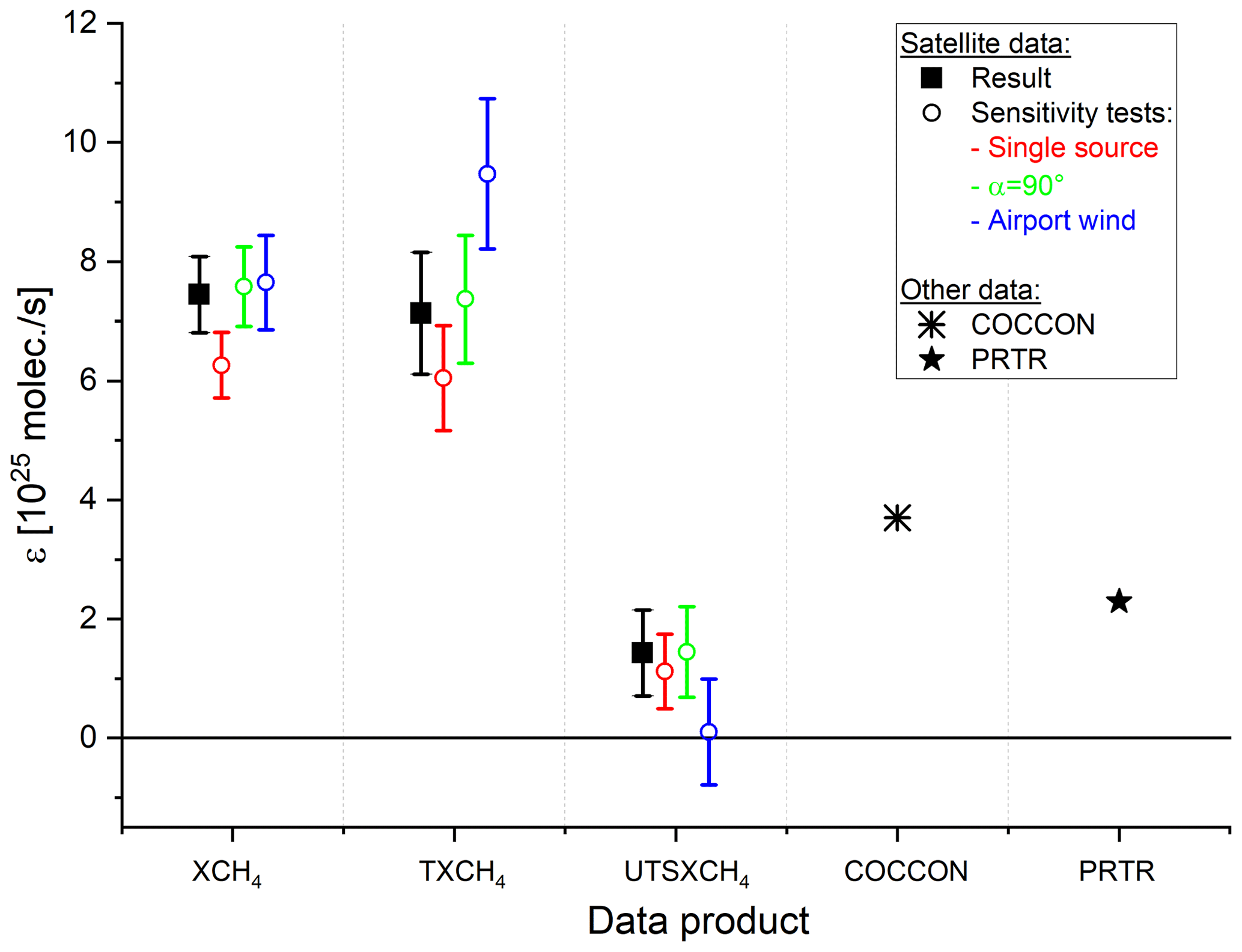
Figure 10Emission strengths for the different products and for the sensitivity tests. Also included are the COCCON observations which characterize the Valdemingómez waste plant contribution and the total of all three sources according to the PRTR inventory.
3.6 Sensitivity study for emission strength estimates
The point sources and their proportion in the total emission rate in this study are based on the a priori knowledge of three different waste plant locations. If we use a single source located at the Pinto waste disposal site only, it yields an emission rate of 6.3 × 1025 molec. s−1, ∼ 15 % lower than that of the three point sources for CH4 and 6.0 × 1025 molec. s−1 (−15 %) for tropospheric CH4 (see Fig. 10). The opening angle (α) is experimentally selected based on the comparison between the TROPOMI measured and modeled NO2 plume, which results in some uncertainties as well. Using 90∘ instead of 60∘ for α in the plume model results in an emission strength of 7.6 × 1025 molec. s−1 (+3 % change) for CH4 and of 7.4 × 1025 molec. s−1 (+4 % change) for tropospheric CH4.
The surface wind can be influenced by the topography, and the actual transport pathway from the emission source to the measurement station is difficult to know (Chen et al., 2016; Babenhauserheide et al., 2020). To study the wind sensitivity, the hourly wind information measured at the Cuatro Vientos Airport at 10 m height is used instead of the ERA5 10 m wind. There are other in situ measurements available but not used here, as the AEMet headquarter station is affected by nearby buildings and the Barajas Airport station is very close to a river (Jarama) that determines a specific wind pattern. The wind measured at the Cuatro Vientos Airport is quite different compared to the ERA5 wind, as in situ-measured NE wind becomes dominant as well, and the wind speed in SW wind field increases by ∼ 50 % compared to that of ERA5 wind (Figs. A3, A4 and Table A1). Using the wind measured at the Cuatro Vientos Airport results in an emission rate of 7.7 × 1025 molec. s−1 (+4 %) for CH4 and 9.5 × 1025 molec. s−1 (+34 %) for tropospheric CH4.
In summary, the uncertainties derived from the source location, opening angle or wind cannot be ignored, but nevertheless the emission rates estimated from the spaceborne observations are clearly larger than the values reported in Table 2 and are larger than the ones estimated from the COCCON SN69 observations in October 2018.
The present study analyzes TROPOMI XCH4 and IASI CH4 retrievals over an area around Madrid for more than 400 d within a rectangle of 39.5–41.5∘ N and 4.5–3.0∘ W (125 km × 220 km) from 10 November 2017 until 10 October 2020. During this time period, a 2-week field campaign was conducted in September 2018 in Madrid, in which five ground-based COCCON instruments were used to measure XCH4 at different locations around the city center.
First, TROPOMI XCH4 is compared with co-located COCCON data from the field campaign, showing a generally good agreement, even though the radius of the collection circle for the satellite measurements was as small as 5 km. However, there are 6 d when obvious enhancements due to local sources were observed by COCCON around noon at the most southeast station (Jose Echegaray), which were underestimated by TROPOMI. The ground-based COCCON observations indicate a local source strength of 3.7 × 1025 molec. s−1 from observations at Jose Echegaray station on 4 October 2018, which is reasonable compared to the emissions assumed for nearby waste plants. The waste plant locations are later used as the point sources to model the emission strength for CH4.
According to the ERA5 model wind at 10 m height, SW (135–315∘) winds (NE covering the remaining wind field) are dominant in the Madrid city center in the time range from November 2017 to October 2020. Based on this wind information, the wind-assigned anomalies are defined as the difference of satellite data between the conditions of the NE wind field and SW wind field. We use the simultaneously measured tropospheric NO2 column amounts from TROPOMI as a proxy to evaluate the wind-assigned anomaly approach due to its short lifetime and clear plume shape, by using ERA5 model wind. Pronounced and bipolar NO2 plumes are observed along the NE–SW wind direction, and a tropospheric NO2 emission strength of 3.5 × 1024 ± 3.9 × 10²² molec. s−1 is estimated. This implies that our method of wind-assigned anomaly is working reliably, that the ERA5 wind data used are indeed representative of the area and the implementation of the satellite data analysis is correct.
CH4 is a long-lived gas and so there are strong CH4 background signals in the atmosphere. Therefore, the background values need to be removed and the anomalies have to be determined before calculating emission strengths. In this study, the removed background values include the linear increase, seasonal cycle, daily variability and horizontal variability. The areas where the three waste plants are located show obvious high anomalies, demonstrating that satellite measurements can detect the local sources after removing the background. Enhanced plumes are more pronounced in the downwind side of SW, whereas the observed downwind plume signal for NE wind is noisier, partly due to the lower number of NE wind situations.
The wind-assigned TROPOMI XCH4 anomalies show a less clear bipolar plume than NO2. This is because CH4 has a long lifetime, and its high background is difficult to totally remove. Based on the wind-assigned anomalies, the emission strength estimated from the TROPOMI XCH4 data is 7.4 × 1025 ± 6.4 × 1024 molec. s−1. In addition, this method is applied to the tropospheric partial column-averaged (ground – 7 km a.s.l.) dry-air molar fractions of methane (TXCH4, obtained by combining TROPOMI and IASI products), yielding an emission strength of 7.1 × 1025 ± 1.0 × 1025 molec. s−1. We show that in the upper troposphere/stratosphere there is no significant plume signal (1.4 × 1025 ± 7.2 × 1024 molec. s−1). The estimation of very similar emission rates from XCH4 and TXCH4 together with the estimated negligible emission rates when using data representing the upper troposphere/stratosphere proves the robustness of our method. The emission rates derived from satellites (XCH4 and TXCH4) are higher than that derived from COCCON observations, as satellites cover larger areas with other CH4 sources and COCCON likely measures local sources.
The surface wind is easily influenced by the topography, which introduces uncertainties in the estimated emission strengths. Using in situ-measured wind at the Cuatro Vientos Airport instead of ERA5 model wind results in an estimated emission rate of 7.7 × 1025 molec. s−1 (+4 %) for CH4 and 9.5 × 1025 molec. s−1 (+34 %) for tropospheric CH4. Uncertainties can also be caused by the choice of the opening angle in the plume model. The estimated emission rates with α=90∘ are 7.6 × 1025 molec. s−1 (+3 %) for CH4 and 7.4 × 1025 molec. s−1 (+4 %) for tropospheric CH4. When using a single source located in the Madrid city center, the emission strengths are 6.3 × 1025 molec. s−1 (−15 %) for CH4 and 6.0 × 1025 molec. s−1 (−15 %) for tropospheric CH4.
In summary, in this study for the first time TROPOMI observations are used together with IASI observations and the ground-based COCCON observations to investigate CH4 emissions from landfills in an important metropolitan area like Madrid. The COCCON instruments show a promising potential for satellite validation and an excellent ability for observation of local sources. The data presented here show that TROPOMI is able to detect the tropospheric NO2 and XCH4 anomalies over metropolitan areas with support from meteorological wind analysis data. This methodology could also be applied to other source regions, space-based sensors and sources of CO2.
Table A1Number of days and the averaged wind speed (±standard deviation) per specific wind area in daytime (08:00–18:00 UTC) from 10 November 2017 to 11 September 2020 measured at the Cuatro Vientos Airport. Columns 2 and 3 are for all days, and columns 4 and 5 are for days with TROPOMI overpass.


Figure A1Examples of wind-assigned NO2 plume based on the simple plume model (ε=5.0 × 1024 molec. s−1) using Madrid as the point source in the NE–SW direction on a 0.1∘ × 0.135∘ latitude–longitude grid with a different opening angle (α) from 10 to 90∘.
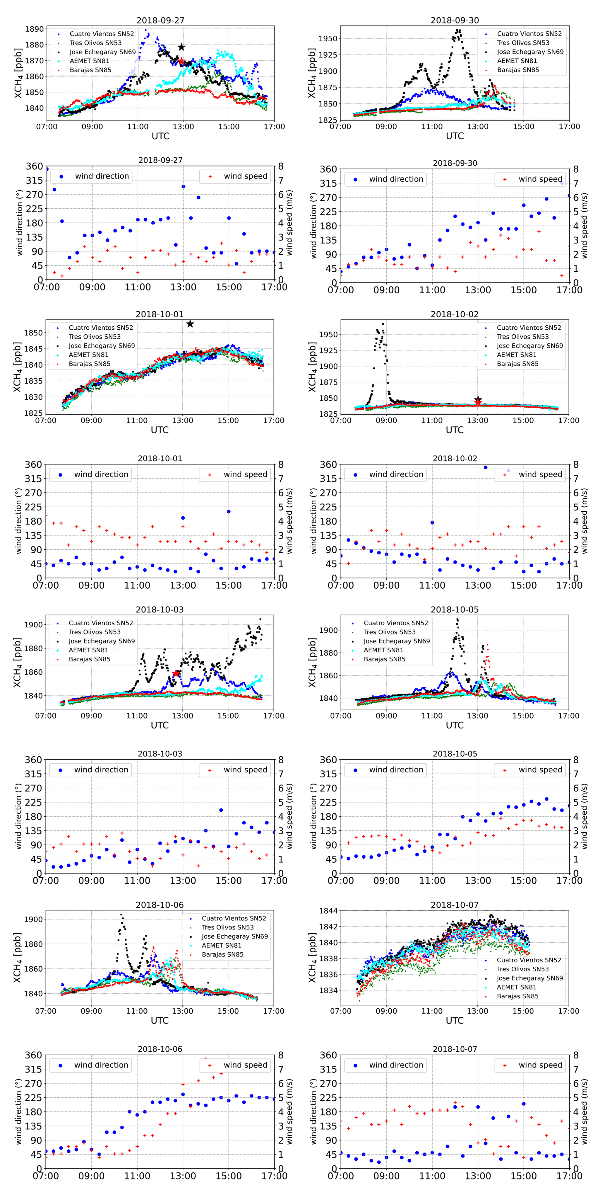
Figure A2Time series of COCCON measurements at five stations and corresponding time series of wind fields (direction and speed) measured at the Cuatro Vientos Airport on 8 d during MEGEI-MAD campaign in 2018. Star symbols represent the TROPOMI observations within a radius of 5 km around each station.
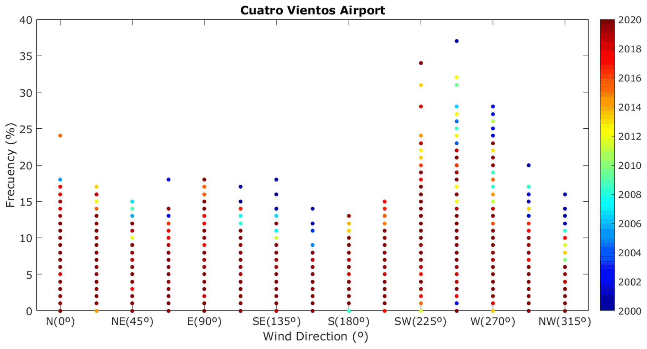
Figure A3Percentage of occurrence for wind direction measured at the Cuatro Vientos Airport between 2000 and 2020. The predominant wind direction is southwest and up to 35 % of time.
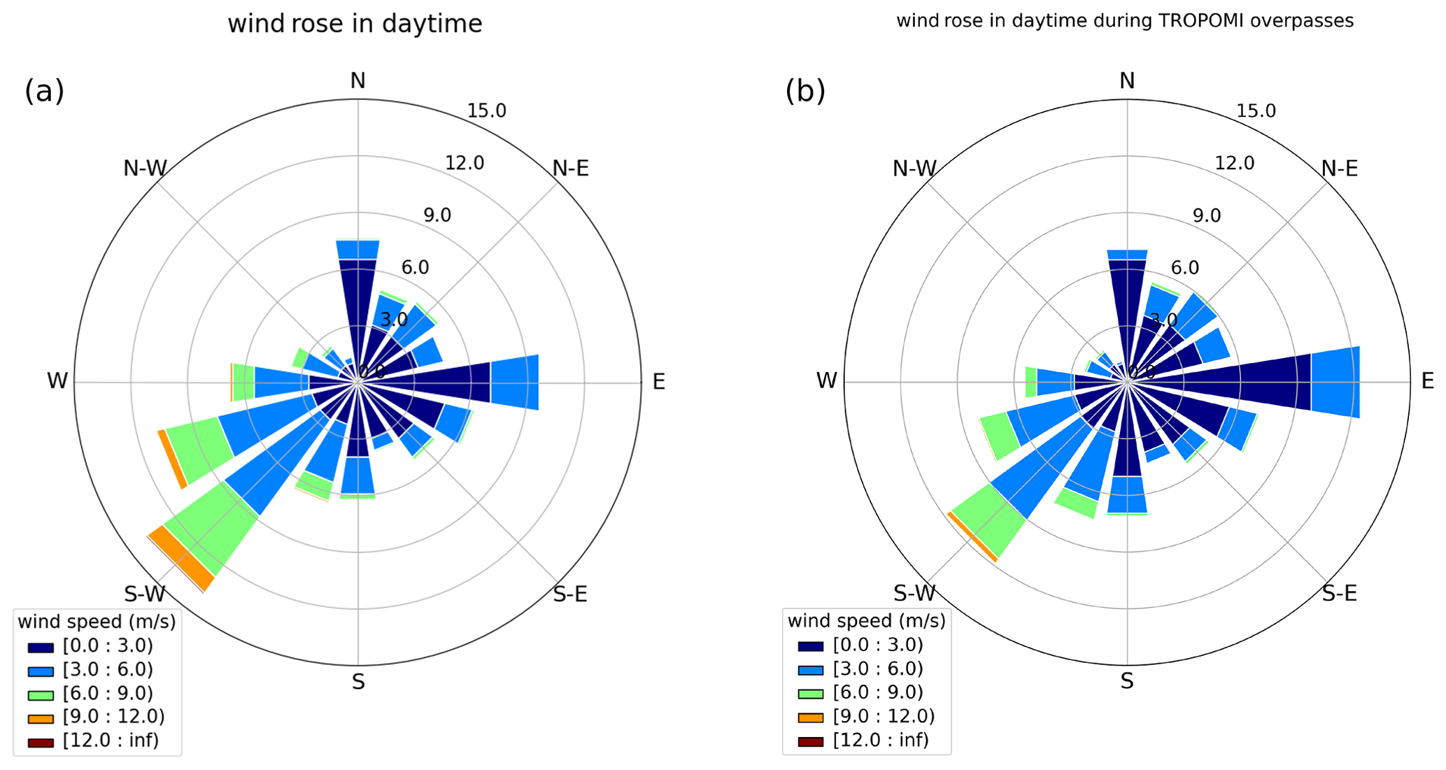
Figure A4Wind roses for daytime (08:00–19:00 UTC) from 10 November 2017 to 11 September 2020 from the wind measurements at the Cuatro Vientos Airport. Panel (a) covers all days and panel (b) covers the days with TROPOMI overpasses.
B1 CH4 background signal
The satellite data can be written as a vector y, where each element corresponds to an individual satellite data point. This signal is caused by a CH4 background signal and the CH4 plume due to the emissions from the waste disposal sites near Madrid:
It is of great importance to adequately separate both components for estimating the emission strength from the satellite data.
For determining the background signal (yBG), we set up a background model:
The matrix KBG is a Jacobian matrix that allows us to reconstruct the background according to a few background model coefficients (the elements of the vector xBG). We also create a Jacobian , which is the same as KBG but set to zero for observations where the wind data suggest a significant impact of the CH4 plume on the satellite data. The calculations of the plume CH4 signals are made according to Sect. 2.3. With the use of we make sure that the estimated background signal is not affected by the CH4 plume.
The KBG is a Jacobian matrix where each row represents an individual satellite observation and each column represents a component of the background model. The background model considers a smooth background, which is a constant CH4 value, a linear increase with time, and a seasonal cycle described by the amplitude and phase of the three frequencies 1/year, 2/year and 3/year. Furthermore, we fit a daily anomaly, which is the same for all data measured during a single day, and a horizontal anomaly, which is the same for any time but dependent on the horizontal location. For the latter we use a 0.1∘ × 0.135∘ (latitude × longitude) grid.
We invert the problem in order to estimate the background model coefficients (elements of the vector xBG):
with GBG being the so-called gain matrix,
Because (and thus GBG) is set to zero whenever yplume=0, we can use in Eq. (B3) y instead of yBG. The matrix Sy,n stands for the noise covariance of the satellite data. For constraining the problem, we use a diagonal (no constraint between different coefficients) with a very low constraint value for the coefficient determining the constant and higher constraint values for the other coefficients. For calculating the uncertainty of the background signal, we calculate the vector and then the mean square value from its elements that represent observations not affected by the plume. This mean square value is then used as the diagonal entries of the diagonal matrix Sy,BG. In this context, Sy,BG considers the deficits of the background model and the uncertainty in the background if determined from data with a certain noise level. As an alternative, we could use modeled high-resolution XCH4 fields (e.g., from CAMS high-resolution greenhouse gas forecast, Barré et al., 2021) for these calculations. We can assume that the model data have no noise and perform an exclusive estimation of the deficits of the background model calculation in form of a full Sy,BG covariance matrix. This more sophisticated uncertainty estimation can be a task for future work.
The uncertainty of the background model coefficients can be calculated as
For each day there is an uncertainty in the background coefficients and the uncertainty is correlated with the uncertainty at other days. All this information is provided in the uncertainty covariance .
With the full Jacobian KBG we can now model the background for the measurement state (also for the measurements that are assumed to be affected by the CH4 waste disposal plume),
and calculate the plume signal according to Eq. (B1) as
The uncertainty of these plume signal is the sum of the uncertainties of the satellite data Sy,n and the uncertainty of the estimated background:
It notes that Eq. (B8) is an approximation, because the two error components are not completely independent (Sy,BG and thus depend also on the noise of the observations; see description for calculating Sy,BG in the context of Eq. B5).
B2 Fitting of CH4 emission rates
Because the CH4 plume signal is rather weak compared to the CH4 background uncertainty and the noise level of the satellite data, we have to work with averages in order to reduce the data noise. The averaging is made by classifying the observation in two predominant wind categories. We calculate the average plume maps for the southwest and northeast wind situations (see Figs. 6 and 8). Then we calculate the difference between the southwest and northeast plume maps (the wind-assigned anomalies or Δ-maps). All the calculations are made by binning all observations that fall within a certain 0.135∘ × 0.1∘ (longitude × latitude) area. In order to significantly reduce the data noise, we only consider averages for the 0.135∘ × 0.1∘ areas based on at least 25 individual observations made under southwest wind conditions and 25 individual observations made under northeast wind conditions. The binning, the averaging, the wind-assigned Δ-maps calculations and the data number filtering are achieved by operator D, and we can write
and
Here Δyplume is a column vector whose elements capture the different signal of the two wind directions at the different locations, and ΔSy,plume is the corresponding uncertainty covariance.
For modeling the plume signals we use a priori knowledge of CH4 emission locations, i.e., assuming a repartition of the emissions between the three waste disposal sites according to Table 2 (see Sect. 3.1). Together with information from the wind, we then model the CH4 plume's wind-assigned anomaly signal Δyplume:
Here the Jacobian Δk (a column vector) represents the wind-assigned anomaly model as described in Sect. 2.3. It describes how an emission at the waste disposal sites according to Table 2 would be seen in the difference signal. We are interested in the coefficient x (a scalar describing how the assumed emissions from Table 2 have to be scaled by a common factor in order to achieve the best agreement with the observed plume).
Similar to Eqs. (B3) and (B4) we write
with the row vector
This fitting of the emission rate correctly considers the respective uncertainty of the difference signals at the different locations.
Because of the small plume signals, it is important to estimate the reliability of the fitted emission rate. The uncertainty of x due to the background uncertainty and the noise in the satellite data can be estimated as
and
respectively. However, as aforementioned these two error components are not completely independent.
The data are accessible by contacting the corresponding author (qiansi.tu@kit.edu). The SRON S5P-RemoTeC scientific TROPOMI CH4 data set from this study is available for download at https://doi.org/10.5281/zenodo.4447228 (Lorente et al., 2021b). The MUSICA IASI data set is available for download via https://doi.org/10.35097/408 (Schneider et al., 2021c).
QT, FH and OG developed the research question. QT wrote the manuscript and performed the data analysis with input from FH, OG, MS and FK. FH suggested the method of constructing wind-assigned anomalies for source quantification. MS suggested the method for calculating the anomalies, for fitting the emission rates and for estimating the uncertainty. OG provided the COCCON and meteorological data and helped to interpret them. TB and AL provided technical support for the TROPOMI data analysis. MS, BE and CJD provided the combined (MUSICA IASI + TROPOMI) data and provided technical support for the analysis of these data. All other coauthors participated in the field campaign and provided the data. All authors discussed the results and contributed to the final paper.
The contact author has declared that neither they nor their co-authors have any competing interests.
Publisher’s note: Copernicus Publications remains neutral with regard to jurisdictional claims in published maps and institutional affiliations.
We would like to thank three anonymous reviewers for their constructive comments and suggestions. We acknowledge ESA support through the COCCON-PROCEEDS and COCCON-PROCEEDS II projects. In addition, this research was funded by the Ministerio de Economía y Competitividad from Spain through the INMENSE project (CGL2016-80688-P). This research has largely benefited from funds of the Deutsche Forschungsgemeinschaft (provided for the two projects MOTIV and TEDDY with IDs/290612604 and 416767181, respectively). Part of this work was performed on the supercomputer ForHLR funded by the Ministry of Science, Research and the Arts Baden-Württemberg and by the German Federal Ministry of Education and Research.
We acknowledge the support by the Deutsche Forschungsgemeinschaft and the Open Access Publishing Fund of the Karlsruhe Institute of Technology.
This research has been supported by the European Space Agency (COCCON-PROCEEDS and COCCON-PROCEEDS II, grant no. ESA-IPL-POELG-cl-LE-2015-1129), the Ministerio de Economía y Competitividad (INMENSE project, grant no. CGL2016-80688-P), the Deutsche Forschungsgemeinschaft (project MOTIV, ID 290612604; and project TEDDY, ID 416767181), the Ministerium für Wissenschaft, Forschung und Kunst Baden-Württemberg (supercomputer ForHLR grant), and the Bundesministerium für Bildung und Forschung (supercomputer ForHLR grant).
The article processing charges for this open-access publication were covered by the Karlsruhe Institute of Technology (KIT).
This paper was edited by Eduardo Landulfo and reviewed by three anonymous referees.
Babenhauserheide, A., Hase, F., and Morino, I.: Net CO2 fossil fuel emissions of Tokyo estimated directly from measurements of the Tsukuba TCCON site and radiosondes, Atmos. Meas. Tech., 13, 2697–2710, https://doi.org/10.5194/amt-13-2697-2020, 2020.
Barré, J., Aben, I., Agustí-Panareda, A., Balsamo, G., Bousserez, N., Dueben, P., Engelen, R., Inness, A., Lorente, A., McNorton, J., Peuch, V.-H., Radnoti, G., and Ribas, R.: Systematic detection of local CH4 anomalies by combining satellite measurements with high-resolution forecasts, Atmos. Chem. Phys., 21, 5117–5136, https://doi.org/10.5194/acp-21-5117-2021, 2021.
Beirle, S., Boersma, K. F., Platt, U., Lawrence, M. G., and Wagner, T.: Megacity Emissions and Lifetimes of Nitrogen Oxides Probed from Space, Science, 333, 1737, https://doi.org/10.1126/science.1207824, 2011.
Bousquet, P., Ciais, P., Miller, J. B., Dlugokencky, E. J., Hauglustaine, D. A., Prigent, C., Van der Werf, G. R., Peylin, P., Brunke, E.-G., Carouge, C., Langenfelds, R. L., Lathière, J., Papa, F., Ramonet, M., Schmidt, M., Steele, L. P., Tyler, S. C., and White, J.: Contribution of anthropogenic and natural sources to atmospheric methane variability, Nature, 443, 439–443, https://doi.org/10.1038/nature05132, 2006.
Butz, A., Hasekamp, O. P., Frankenberg, C., and Aben, I.: Retrievals of atmospheric CO2 from simulated space-borne measurements of backscattered near-infrared sunlight: accounting for aerosol effects, Appl. Opt., 48, 3322–3336, 2009.
Butz, A., Guerlet, S., Hasekamp, O., Schepers, D., Galli, A., Aben, I., Frankenberg, C., Hartmann, J.-M., Tran, H., Kuze, A., Keppel-Aleks, G., Toon, G., Wunch, D., Wennberg, P., Deutscher, N., Griffith, D., Macatangay, R., Messerschmidt, J., Notholt, J., and Warneke, T.: Toward accurate CO2 and CH4 observations from GOSAT, Geophys. Res. Lett., 38, L14812, https://doi.org/10.1029/2011GL047888, 2011.
Butz, A., Dinger, A. S., Bobrowski, N., Kostinek, J., Fieber, L., Fischerkeller, C., Giuffrida, G. B., Hase, F., Klappenbach, F., Kuhn, J., Lübcke, P., Tirpitz, L., and Tu, Q.: Remote sensing of volcanic CO2, HF, HCl, SO2, and BrO in the downwind plume of Mt. Etna, Atmos. Meas. Tech., 10, 1–14, https://doi.org/10.5194/amt-10-1-2017, 2017.
Cambaliza, M. O. L., Shepson, P. B., Bogner, J., Caulton, D. R., Stirm, B., Sweeney, C., Montzka, S. A., Gurney, K. R., Spokas, K., Salmon, O. E., Lavoie, T. N., Hendricks, A., Mays, K., Turnbull, J., Miller, B. R., Lauvaux, T., Davis, K., Karion, A., Moser, B., Miller, C., Obermeyer, C., Whetstone, J., Prasad, K., Miles, N., and Richardson, S.: Quantification and source apportionment of the methane emission flux from the city of Indianapolis, Elementa: Science of the Anthropocene, 3, 000037, https://doi.org/10.12952/journal.elementa.000037, 2015.
Chen, J., Viatte, C., Hedelius, J. K., Jones, T., Franklin, J. E., Parker, H., Gottlieb, E. W., Wennberg, P. O., Dubey, M. K., and Wofsy, S. C.: Differential column measurements using compact solar-tracking spectrometers, Atmos. Chem. Phys., 16, 8479–8498, https://doi.org/10.5194/acp-16-8479-2016, 2016.
Chynoweth, D. P., Owens, J. M., and Legrand, R.: Renewable methane from anaerobic digestion of biomass, Renew. Energy, 22, 1–8, https://doi.org/10.1016/S0960-1481(00)00019-7, 2001.
Copernicus Climate Change Service (C3S): ERA5: Fifth generation of ECMWF atmospheric reanalyses of the global climate, Copernicus Climate Change Service Climate Data Store (CDS), available at: https://cds.climate.copernicus.eu/cdsapp#!/home (last access: 22 December 2021), 2017.
Crippa, M., Oreggioni, G., Guizzardi, D., Muntean, M., Schaaf, E., Lo Vullo, E., Solazzo, E., Monforti-Ferrario, F., Olivier, J. G. J., and Vignati, E.: Fossil CO2 and GHG emissions of all world countries – 2019 Report, EUR 29849 EN, Publications Office of the European Union, Luxembourg, JRC117610, https://doi.org/10.2760/687800, ISBN 978-92-76-11100-9, 2019.
De Gouw, J. A., Veefkind, J. P., Roosenbrand, E., Dix, B., Lin, J. C., Landgraf, J., and Levelt, P. F.: Daily Satellite Observations of Methane from Oil and Gas Production Regions in the United States, Scientific Reports, 10, 1379, https://doi.org/10.1038/s41598-020-57678-4, 2020.
Delkash, M, Zhou, B., Han, B., Chow, F. K., Rella, C. W., and Imhoff, P. T.: Short-term landfill methane emissions dependency on wind, Waste Manage., 55, 288–298, https://doi.org/10.1016/j.wasman.2016.02.009, 2016.
De Wachter, E., Kumps, N., Vandaele, A. C., Langerock, B., and De Mazière, M.: Retrieval and validation of MetOp/IASI methane, Atmos. Meas. Tech., 10, 4623–4638, https://doi.org/10.5194/amt-10-4623-2017, 2017.
Dietrich, F., Chen, J., Voggenreiter, B., Aigner, P., Nachtigall, N., and Reger, B.: MUCCnet: Munich Urban Carbon Column network, Atmos. Meas. Tech., 14, 1111–1126, https://doi.org/10.5194/amt-14-1111-2021, 2021.
Etminan, M., Myhre, G., Highwood, E. J., and Shine, K. P., Radiative forcing of carbon dioxide, methane, and nitrous oxide: A significant revision of the methane radiative forcing, Geophys. Res. Lett., 43, 12614–12623, https://doi.org/10.1002/2016GL071930, 2016.
Farr, T. G., Rosen, P. A., Caro, E., Crippen, R., Duren, R., Hensley, S., Kobrick, M., Paller, M., Rodriguez, E., Roth, L., Seal, D., Shaffer, S., Shimada, J., Umland, J., Werner, M., Oskin, M., Burbank, D., and Alsdorf, D.: The Shuttle Radar Topography Mission, Rev. Geophys., 45, RG2004, https://doi.org/10.1029/2005RG000183, 2007.
Frey, M., Hase, F., Blumenstock, T., Groß, J., Kiel, M., Mengistu Tsidu, G., Schäfer, K., Sha, M. K., and Orphal, J.: Calibration and instrumental line shape characterization of a set of portable FTIR spectrometers for detecting greenhouse gas emissions, Atmos. Meas. Tech., 8, 3047–3057, https://doi.org/10.5194/amt-8-3047-2015, 2015.
Frey, M., Sha, M. K., Hase, F., Kiel, M., Blumenstock, T., Harig, R., Surawicz, G., Deutscher, N. M., Shiomi, K., Franklin, J. E., Bösch, H., Chen, J., Grutter, M., Ohyama, H., Sun, Y., Butz, A., Mengistu Tsidu, G., Ene, D., Wunch, D., Cao, Z., Garcia, O., Ramonet, M., Vogel, F., and Orphal, J.: Building the COllaborative Carbon Column Observing Network (COCCON): long-term stability and ensemble performance of the EM27/SUN Fourier transform spectrometer, Atmos. Meas. Tech., 12, 1513–1530, https://doi.org/10.5194/amt-12-1513-2019, 2019.
García, O. E., Schneider, M., Ertl, B., Sepúlveda, E., Borger, C., Diekmann, C., Wiegele, A., Hase, F., Barthlott, S., Blumenstock, T., Raffalski, U., Gómez-Peláez, A., Steinbacher, M., Ries, L., and de Frutos, A. M.: The MUSICA IASI CH4 and N2O products and their comparison to HIPPO, GAW and NDACC FTIR references, Atmos. Meas. Tech., 11, 4171–4215, https://doi.org/10.5194/amt-11-4171-2018, 2018.
García, O., Morgui, J.-A., Curcoll, R., Estruch, C., Sepúlveda, E., Ramos, R., and Cuevas, E.: Characterizing methane emissions in Madrid City within the MEGEI-MAD project: the temporal and spatial ground-based mobile approach, 8th International Symposium on Non-CO2 Greenhouse Gases (NCGG8), Amsterdam (The Netherlands), 12–14 June, 2019.
García, O. E., Sepúlveda, E., León-Luis, S. F., Morgui, J.-A., Frey, M., Schneider, C., Ramos, R., Torres, C., Curcoll, R., Estruch, C., Barreto, Á., Toledano, C., Hase, F., Butz, A., Cuevas, E., Blumenstock, T., Bustos, J. J., and Marrero, C.: Monitoring of Greenhouse Gas and Aerosol Emissions in Madrid megacity (MEGEI-MAD), GAW Symposium 2021 (online), 28 June–2 July, 2021.
Gisi, M., Hase, F., Dohe, S., Blumenstock, T., Simon, A., and Keens, A.: XCO2-measurements with a tabletop FTS using solar absorption spectroscopy, Atmos. Meas. Tech., 5, 2969–2980, https://doi.org/10.5194/amt-5-2969-2012, 2012.
Guerlet, S., Butz, A., Schepers, D., Basu, S., Hasekamp, O. P., Kuze, A., Yokota, T., Blavier, J.-F., Deutscher, N. M., Griffith, D. W. T., Hase, F., Kyro, E., Morino, I., Sherlock, V., Sussmann, R., Galli, A., and Aben, I.: Impact of aerosol and thin cirrus on retrieving and validating XCO2 from GOSAT shortwave infrared measurements, J. Geophys. Res.-Atmos., 118, 4887–4905, https://doi.org/10.1002/jgrd.50332, 2013.
Hase, F., Frey, M., Blumenstock, T., Groß, J., Kiel, M., Kohlhepp, R., Mengistu Tsidu, G., Schäfer, K., Sha, M. K., and Orphal, J.: Application of portable FTIR spectrometers for detecting greenhouse gas emissions of the major city Berlin, Atmos. Meas. Tech., 8, 3059–3068, https://doi.org/10.5194/amt-8-3059-2015, 2015.
Hase, F., Frey, M., Kiel, M., Blumenstock, T., Harig, R., Keens, A., and Orphal, J.: Addition of a channel for XCO observations to a portable FTIR spectrometer for greenhouse gas measurements, Atmos. Meas. Tech., 9, 2303–2313, https://doi.org/10.5194/amt-9-2303-2016, 2016.
Hasekamp, O., Lorente, A., Hu, H., Butz, A., aan de Brugh, J., and Landgraf, J.: Algorithm Theoretical Baseline Document for Sentinel-5 Precursor methane retrieval, available at: https://sentinel.esa.int/documents/247904/2476257/Sentinel-5P-TROPOMI-ATBD-Methane-retrieval (last access: 22 December 2022), 2021.
Hasekamp, O. P. and Butz, A.: Efficient calculation of intensity and polarization spectra in vertically inhomogeneous scattering and absorbing atmospheres, J. Geophys. Res., 113, D20309, https://doi.org/10.1029/2008JD010379, 2008.
Hu, H., Hasekamp, O., Butz, A., Galli, A., Landgraf, J., Aan de Brugh, J., Borsdorff, T., Scheepmaker, R., and Aben, I.: The operational methane retrieval algorithm for TROPOMI, Atmos. Meas. Tech., 9, 5423–5440, https://doi.org/10.5194/amt-9-5423-2016, 2016.
Hu, H., Landgraf, J., Detmers, R., Borsdorff, T., Brugh, J. A. d., Aben, I., Butz, A., and Hasekamp, O.: Toward Global Mapping of Methane With TROPOMI: First Results and Intersatellite Comparison to GOSAT, Geophys. Res. Lett., 45, 3682–3689, https://doi.org/10.1002/2018GL077259, 2018.
Jacobs, N., Simpson, W. R., Wunch, D., O'Dell, C. W., Osterman, G. B., Hase, F., Blumenstock, T., Tu, Q., Frey, M., Dubey, M. K., Parker, H. A., Kivi, R., and Heikkinen, P.: Quality controls, bias, and seasonality of CO2 columns in the boreal forest with Orbiting Carbon Observatory-2, Total Carbon Column Observing Network, and EM27/SUN measurements, Atmos. Meas. Tech., 13, 5033–5063, https://doi.org/10.5194/amt-13-5033-2020, 2020.
Kenagy, H. S., Sparks, T. L., Ebben, C. J., Wooldrige, P. J., Lopez-Hilfiker, F. D., Lee, B. H., Thornton, J. A., McDuffie, E. E., Fibiger, D. L., Brown, S. S., Montzka, D. D., Weinheimer, A. J., Schroder, J. C., Campuzano-Jost, P., Day, D. A., Jimenez, J. L., Dibb, J. E., Campos, T., Shah, V., Jaeglé, L., and Cohen, R. C.: NOx Lifetime and NOy Partitioning During WINTER, J. Geophys. Res.-Atmos., 123, 9813–9827, https://doi.org/10.1029/2018JD028736, 2018.
Kirschke, S., Bousquet, P., Ciais, P., Saunois, M., Canadell, J., Dlugokencky, E., Bergamaschi, P., Bergmann, D., Blake, D., Bruhwiler, L., Cameron-Smith, P., Castaldi, S., Chevallier, F., Feng, L., Fraser, A., Heimann, M., Hodson, E., Houweling, S., Josse, B., Fraser, P., Krummel, P., Lamarque, J.-F., Langenfelds, R., Le Quere, C., Naik, V., O'Doherty, S., Palmer, P., Pison, I., Plummer, D., Poulter, B., Prinn, R., Rigby, M., Ringeval, B., Santini, M., Schmidt, M., Shindell, D., Simpson, I., Spahni, R., Steele, L., Strode, S., Sudo, K., Szopa, S., Van Der Werf, G., Voulgarakis, A., Van Weele, M., Weiss, R., Williams, J., and Zeng, G.: Three decades of global methane sources and sinks, Nat. Geosci., 6, 813–823, https://doi.org/10.1038/ngeo1955, 2013.
Klappenbach, F., Bertleff, M., Kostinek, J., Hase, F., Blumenstock, T., Agusti-Panareda, A., Razinger, M., and Butz, A.: Accurate mobile remote sensing of XCO2 and XCH4 latitudinal transects from aboard a research vessel, Atmos. Meas. Tech., 8, 5023–5038, https://doi.org/10.5194/amt-8-5023-2015, 2015.
Kulawik, S. S., Worden, J. R., Payne, V. H., Fu, D., Wofsy, S. C., McKain, K., Sweeney, C., Daube Jr., B. C., Lipton, A., Polonsky, I., He, Y., Cady-Pereira, K. E., Dlugokencky, E. J., Jacob, D. J., and Yin, Y.: Evaluation of single-footprint AIRS CH4 profile retrieval uncertainties using aircraft profile measurements, Atmos. Meas. Tech., 14, 335–354, https://doi.org/10.5194/amt-14-335-2021, 2021.
Landgraf, J., Butz, A., Hasekamp, O., Hu, H., and aan de Brugh, J.: Sentinel 5 L2 Prototype Processors, Algorithm Theoretical Baseline Document: Methane Retrieval, SRON-ESA-S5L2PPATBD-001-v3.1-20190517-CH4, SRON Netherlands Institute for Space Research, Utrecht, the Netherlands, 2019.
Lorente, A., Borsdorff, T., Butz, A., Hasekamp, O., aan de Brugh, J., Schneider, A., Wu, L., Hase, F., Kivi, R., Wunch, D., Pollard, D. F., Shiomi, K., Deutscher, N. M., Velazco, V. A., Roehl, C. M., Wennberg, P. O., Warneke, T., and Landgraf, J.: Methane retrieved from TROPOMI: improvement of the data product and validation of the first 2 years of measurements, Atmos. Meas. Tech., 14, 665–684, https://doi.org/10.5194/amt-14-665-2021, 2021a.
Lorente, A., Borsdorff, T., aan de Brugh, J., Landgraf, J., and Hasekamp, O.: SRON S5P – RemoTeC scientific TROPOMI XCH4 dataset, Zenodo [data set], https://doi.org/10.5281/zenodo.4447228, 2021b.
Luther, A., Kleinschek, R., Scheidweiler, L., Defratyka, S., Stanisavljevic, M., Forstmaier, A., Dandocsi, A., Wolff, S., Dubravica, D., Wildmann, N., Kostinek, J., Jöckel, P., Nickl, A.-L., Klausner, T., Hase, F., Frey, M., Chen, J., Dietrich, F., Nȩcki, J., Swolkień, J., Fix, A., Roiger, A., and Butz, A.: Quantifying CH4 emissions from hard coal mines using mobile sun-viewing Fourier transform spectrometry, Atmos. Meas. Tech., 12, 5217–5230, https://doi.org/10.5194/amt-12-5217-2019, 2019.
Pandey, S., Gautam, R., Houweling, S., van der Gon, H. D., Sadavarte, P., Borsdorff, T., Hasekamp, O., Landgraf, J., Tol, P., van Kempen, T., Hoogeveen, R., van Hees, R., Hamburg, S. P., Maasakkers, J. D., and Aben, I.: Satellite observations reveal extreme methane leakage from a natural gas well blowout, P. Natl. Acad. Sci. USA, 116, 26376, https://doi.org/10.1073/pnas.1908712116, 2019.
Rachor, I. M., Gebert, J., Gröngröft, A., and Pfeiffer, E.-M.: Variability of methane emissions from an old landfill over different time-scales, Eur. J. Soil Sci., 64, 16–26, https://doi.org/10.1111/ejss.12004, 2013.
Sánchez, C., de la Fuente, M. del M., Narros, A., del Peso, I., and Rodríguez, E.: Comparison of modeling with empirical calculation of diffuse and fugitive methane emissions in a Spanish landfill, J. Air Waste Manage. Assoc., 69, 362–372, https://doi.org/10.1080/10962247.2018.1541029, 2019.
Saunois, M., Stavert, A. R., Poulter, B., Bousquet, P., Canadell, J. G., Jackson, R. B., Raymond, P. A., Dlugokencky, E. J., Houweling, S., Patra, P. K., Ciais, P., Arora, V. K., Bastviken, D., Bergamaschi, P., Blake, D. R., Brailsford, G., Bruhwiler, L., Carlson, K. M., Carrol, M., Castaldi, S., Chandra, N., Crevoisier, C., Crill, P. M., Covey, K., Curry, C. L., Etiope, G., Frankenberg, C., Gedney, N., Hegglin, M. I., Höglund-Isaksson, L., Hugelius, G., Ishizawa, M., Ito, A., Janssens-Maenhout, G., Jensen, K. M., Joos, F., Kleinen, T., Krummel, P. B., Langenfelds, R. L., Laruelle, G. G., Liu, L., Machida, T., Maksyutov, S., McDonald, K. C., McNorton, J., Miller, P. A., Melton, J. R., Morino, I., Müller, J., Murguia-Flores, F., Naik, V., Niwa, Y., Noce, S., O'Doherty, S., Parker, R. J., Peng, C., Peng, S., Peters, G. P., Prigent, C., Prinn, R., Ramonet, M., Regnier, P., Riley, W. J., Rosentreter, J. A., Segers, A., Simpson, I. J., Shi, H., Smith, S. J., Steele, L. P., Thornton, B. F., Tian, H., Tohjima, Y., Tubiello, F. N., Tsuruta, A., Viovy, N., Voulgarakis, A., Weber, T. S., van Weele, M., van der Werf, G. R., Weiss, R. F., Worthy, D., Wunch, D., Yin, Y., Yoshida, Y., Zhang, W., Zhang, Z., Zhao, Y., Zheng, B., Zhu, Q., Zhu, Q., and Zhuang, Q.: The Global Methane Budget 2000–2017, Earth Syst. Sci. Data, 12, 1561–1623, https://doi.org/10.5194/essd-12-1561-2020, 2020.
Schneider, M., Ertl, B., Diekmann, C. J., Khosrawi, F., Röhling, A. N., Hase, F., Dubravica, D., García, O. E., Sepúlveda, E., Borsdorff, T., Landgraf, J., Lorente, A., Chen, H., Kivi, R., Laemmel, T., Ramonet, M., Crevoisier, C., Pernin, J., Steinbacher, M., Meinhardt, F., Deutscher, N. M., Griffith, D. W. T., Velazco, V. A., and Pollard, D. F.: Synergetic use of IASI and TROPOMI space borne sensors for generating a tropospheric methane profile product, Atmos. Meas. Tech. Discuss. [preprint], https://doi.org/10.5194/amt-2021-31, in review, 2021a.
Schneider, M., Ertl, B., Diekmann, C. J., Khosrawi, F., Weber, A., Hase, F., Höpfner, M., García, O. E., Sepúlveda, E., and Kinnison, D.: Design and description of the MUSICA IASI full retrieval product, Earth Syst. Sci. Data Discuss. [preprint], https://doi.org/10.5194/essd-2021-75, in review, 2021b.
Schneider, M., Ertl, B., and Diekmann, C.: MUSICA IASI full retrieval product standard output (processing version 3.2.1). Institute of Meteorology and Climate Reasearch, Atmospheric Trace Gases and Remote Sensing (IMK-ASF), Karlsruhe Institute of Technology (KIT), https://doi.org/10.35097/408, 2021c.
Schneising, O., Buchwitz, M., Reuter, M., Vanselow, S., Bovensmann, H., and Burrows, J. P.: Remote sensing of methane leakage from natural gas and petroleum systems revisited, Atmos. Chem. Phys., 20, 9169–9182, https://doi.org/10.5194/acp-20-9169-2020, 2020.
Sha, M. K., De Mazière, M., Notholt, J., Blumenstock, T., Chen, H., Dehn, A., Griffith, D. W. T., Hase, F., Heikkinen, P., Hermans, C., Hoffmann, A., Huebner, M., Jones, N., Kivi, R., Langerock, B., Petri, C., Scolas, F., Tu, Q., and Weidmann, D.: Intercomparison of low- and high-resolution infrared spectrometers for ground-based solar remote sensing measurements of total column concentrations of CO2, CH4, and CO, Atmos. Meas. Tech., 13, 4791–4839, https://doi.org/10.5194/amt-13-4791-2020, 2020.
Shah, V., Jacob, D. J., Li, K., Silvern, R. F., Zhai, S., Liu, M., Lin, J., and Zhang, Q.: Effect of changing NOx lifetime on the seasonality and long-term trends of satellite-observed tropospheric NO2 columns over China, Atmos. Chem. Phys., 20, 1483–1495, https://doi.org/10.5194/acp-20-1483-2020, 2020.
Siddans, R., Knappett, D., Kerridge, B., Waterfall, A., Hurley, J., Latter, B., Boesch, H., and Parker, R.: Global height-resolved methane retrievals from the Infrared Atmospheric Sounding Interferometer (IASI) on MetOp, Atmos. Meas. Tech., 10, 4135–4164, https://doi.org/10.5194/amt-10-4135-2017, 2017.
Solazzo, E., Crippa, M., Guizzardi, D., Muntean, M., Choulga, M., and Janssens-Maenhout, G.: Uncertainties in the Emissions Database for Global Atmospheric Research (EDGAR) emission inventory of greenhouse gases, Atmos. Chem. Phys., 21, 5655–5683, https://doi.org/10.5194/acp-21-5655-2021, 2021.
Tu, Q., Hase, F., Blumenstock, T., Kivi, R., Heikkinen, P., Sha, M. K., Raffalski, U., Landgraf, J., Lorente, A., Borsdorff, T., Chen, H., Dietrich, F., and Chen, J.: Intercomparison of atmospheric CO2 and CH4 abundances on regional scales in boreal areas using Copernicus Atmosphere Monitoring Service (CAMS) analysis, COllaborative Carbon Column Observing Network (COCCON) spectrometers, and Sentinel-5 Precursor satellite observations, Atmos. Meas. Tech., 13, 4751–4771, https://doi.org/10.5194/amt-13-4751-2020, 2020a.
Tu, Q., Hase, F., Blumenstock, T., Schneider, M., Schneider, A., Kivi, R., Heikkinen, P., Ertl, B., Diekmann, C., Khosrawi, F., Sommer, M., Borsdorff, T., and Raffalski, U.: Intercomparison of arctic XH2O observations from three ground-based Fourier transform infrared networks and application for satellite validation, Atmos. Meas. Tech., 14, 1993–2011, https://doi.org/10.5194/amt-14-1993-2021, 2021b.
Varon, D. J., McKeever, J., Jervis, D., Maasakkers, J. D., Pandey, S., Houweling, S., Aben, I., Scarpelli, T., and Jacob, D. J. : Satellite discovery of anomalously large methane point sources from oil/gas production, Geophys. Res. Lett., 46, 13507–13516, https://doi.org/10.1029/2019GL083798, 2019.
Varon, D. J., Jacob, D. J., Jervis, D., and McKeever, J.: Quantifying Time-Averaged Methane Emissions from Individual Coal Mine Vents with GHGSat-D Satellite Observations, Environ. Sci. Technol., 54, 10246–10253, https://doi.org/10.1021/acs.est.0c01213, 2020.
Vogel, F. R., Frey, M., Staufer, J., Hase, F., Broquet, G., Xueref-Remy, I., Chevallier, F., Ciais, P., Sha, M. K., Chelin, P., Jeseck, P., Janssen, C., Té, Y., Groß, J., Blumenstock, T., Tu, Q., and Orphal, J.: XCO2 in an emission hot-spot region: the COCCON Paris campaign 2015, Atmos. Chem. Phys., 19, 3271–3285, https://doi.org/10.5194/acp-19-3271-2019, 2019.
Washenfelder, R. A., Toon, G. C., Blavier, J.-F., Yang, Z., Allen, N. T., Wennberg, P. O., Vay, S. A., Matross, D. M., and Daube, B. C.: Carbon dioxide column abundances at the Wisconsin Tall Tower site, J. Geophys. Res., 111, D22305, https://doi.org/10.1029/2006JD007154, 2006.
World Meteorological Organization: WMO Greenhouse Gases Bulletin: The State of Greenhouse Gases in the Atmosphere Based on Global Observations through 2019. No. 16, available at: https://reliefweb.int/sites/reliefweb.int/files/resources/GHG-Bulletin-16_en.pdf (last access: 10 January 2020), 2020.
Wunch, D., Toon, G. C., Blavier, J.-F. L., Washenfelder, R. A., Notholt, J., Connor, B. J., Griffith, D. W. T., Sherlock, V., and Wennberg, P. O.: The total carbon column observing network, Philos. T. Roy. Soc. A, 369, 2087–2112, https://doi.org/10.1098/rsta.2010.0240, 2011.
Wunch, D., Toon, G. C., Sherlock, V., Deutscher, N. M., Liu, C., Feist, D. G., and Wennberg, P. O.: The Total Carbon Column Observing Network's GGG2014 Data Version, Tech. rep., California Institute of Technology, Pasadena, California, https://doi.org/10.14291/tccon.ggg2014.documentation.R0/ 1221662, 2015.