the Creative Commons Attribution 4.0 License.
the Creative Commons Attribution 4.0 License.
 | 24 Feb 2022
Plant gross primary production, plant respiration and carbonyl sulfide emissions over the globe inferred by atmospheric inverse modelling
Frédéric Chevallier
Fabienne Maignan
Sauveur Belviso
Antoine Berchet
Alexandra Parouffe
Camille Abadie
Cédric Bacour
Sinikka Lennartz
Philippe Peylin
Carbonyl sulfide (COS), a trace gas showing striking similarity to CO2 in terms of biochemical diffusion pathway into leaves, has been recognized as a promising indicator of the plant gross primary production (GPP), the amount of carbon dioxide that is absorbed through photosynthesis by terrestrial ecosystems. However, large uncertainties about the other components of its atmospheric budget prevent us from directly relating the atmospheric COS measurements to GPP. The largest uncertainty comes from the closure of its atmospheric budget, with a source component missing. Here, we explore the benefit of assimilating both COS and CO2 measurements into the LMDz atmospheric transport model to obtain consistent information on GPP, plant respiration and COS budget. To this end, we develop an analytical inverse system that optimizes biospheric fluxes for the 15 plant functional types (PFTs) defined in the ORCHIDEE global land surface model. Plant uptake of COS is parameterized as a linear function of GPP and of the leaf relative uptake (LRU), which is the ratio of COS to CO2 deposition velocities in plants. A possible scenario for the period 2008–2019 leads to a global biospheric sink of 800 GgS yr−1, with higher absorption in the high latitudes and higher oceanic emissions between 400 and 600 GgS yr−1 most of which is located in the tropics. As for the CO2 budget, the inverse system increases GPP in the high latitudes by a few GtC yr−1 without modifying the respiration compared to the ORCHIDEE fluxes used as a prior. In contrast, in the tropics the system tends to weaken both respiration and GPP. The optimized components of the COS and CO2 budgets have been evaluated against independent measurements over North America, the Pacific Ocean, at three sites in Japan and at one site in France. Overall, the posterior COS concentrations are in better agreement with the COS retrievals at 250 hPa from the MIPAS satellite and with airborne measurements made over North America and the Pacific Ocean. The system seems to have rightly corrected the underestimated GPP over the high latitudes. However, the change in seasonality of GPP in the tropics disagrees with solar-induced fluorescence (SIF) data. The decline in biospheric sink in the Amazon driven by the inversion also disagrees with MIPAS COS retrievals at 250 hPa, highlighting the lack of observational constraints in this region. Moreover, the comparison with the surface measurements in Japan and France suggests misplaced sources in the prior anthropogenic inventory, emphasizing the need for an improved inventory to better partition oceanic and continental sources in Asia and Europe.
- Article
(6332 KB) - Full-text XML
-
Supplement
(1699 KB) - BibTeX
- EndNote


Globally, the amount of carbon assimilated by plant photosynthesis, known as gross primary productivity (GPP), exceeds plant respiration by a few GtC yr−1, which allows terrestrial ecosystems to be a global sink for CO2 in the atmosphere. By absorbing a quarter of the atmospheric carbon dioxide (CO2) emitted by human activities, terrestrial ecosystems help to mitigate the increasing CO2 concentration in the atmosphere, the main driver of climate change (Friedlingstein et al., 2020). The spatial distribution of this carbon sink remains uncertain and a subject of intensive research. This is obviously also the case for its components, GPP and respiration. For these gross fluxes, the uncertainty on the seasonal variations and the overall magnitude are also very large (Anav et al., 2015).
The two most common methods for estimating ecosystem-wide GPP and respiration are based on eddy covariance measurements and land surface models (LSMs). While eddy covariance measurements, on one hand, can be used to routinely estimate GPP and respiration at the local scale, their extrapolation to a whole biome is not straightforward due to their small footprint (Jung et al., 2020). Land surface models (LSMs), on the other hand, have global coverage but represent processes that are not well described and are therefore heavily tuned (Kuppel et al., 2012). For instance, LSMs disagree on the representation of the large spatial and temporal variability of the CO2 gross and net fluxes (Anav et al., 2015). Satellite retrievals of, e.g., solar-induced fluorescence (SIF) or normalized difference vegetation index (NDVI) (Joiner et al., 2016) are also used to constrain GPP. However, remote sensing methods rely on a number of assumptions to convert satellite-measured photons to on-the-ground photosynthesis (Sun et al., 2018). Therefore, there is a need for new information about GPP or respiration to ensure a better partitioning between these components of the CO2 atmospheric budget.
Carbonyl sulfide (COS) is recognized as a promising tracer of GPP at the leaf scale (Stimler et al., 2010; Seibt et al., 2010) and at a large scale (Campbell et al., 2008; Blake et al., 2008). COS follows the same diffusion pathway from the leaf boundary layer to the plant cells where photosynthesis takes place. However, while CO2 is re-emitted into the atmosphere through respiration, COS is nearly irreversibly hydrolysed in a reaction catalysed by the enzyme carbonic anhydrase (CA) (Protoschill-Krebs et al., 1996). Therefore, the atmospheric drawdown of COS reflects the uptake of COS by the plant to a large extent. Despite this property, COS measurements cannot easily be used in inverse modelling to constrain GPP because the other terms of the COS atmospheric budget are also poorly quantified, to the point that the bottom-up COS atmospheric budget is even less closed than the bottom-up CO2 atmospheric budget. The process description of all components of the COS budget (i.e., bottom-up budget) suggests a decreasing concentration of COS, but the latter has been relatively stable around 500 parts per trillion (ppt, 1 ppt is 10−12 mol mol−1) over the past 30 years (Whelan et al., 2018). The current notion is that there is a “missing” source in the current atmospheric COS budget, likely in the tropics (Montzka et al., 2007; Glatthor et al., 2015; Berry et al., 2013a).
The terrestrial sink induced by both plants and soils has been estimated between 500–1200 GgS yr−1 consistent with the large COS deficit seen in airborne profiles in the Northern Hemisphere (Campbell et al., 2008; Suntharalingam et al., 2008; Berry et al., 2013a). Soil uptake, resulting from the presence of CA in soil microorganisms, is thought to be much smaller in magnitude than vegetation fluxes (Whelan et al., 2018). In the atmosphere, COS also has two chemical sinks: models indicate that about 100 GgS yr−1 of COS is oxidized by OH in the low troposphere while 50 ± 15 GgS yr−1 is photolysed in the stratosphere (Whelan et al., 2018). The largest sources of COS are from human activities and the ocean, with minor contributions from biomass burning (50–100 GgS yr−1, Glatthor et al., 2017; Stinecipher et al., 2019). The oceanic source has been estimated between 200 and 400 GgS yr−1 (Lennartz et al., 2017, 2020a). The missing source is unlikely to arise from direct ocean emissions since the ship cruises have recorded a sub-saturation of tropical sea waters with respect to COS (Lennartz et al., 2017). COS production from atmospheric oxidation of dimethyl sulfide (DMS) and carbon disulfide (CS2) are two other candidates that may support the missing source, as they have been reported to peak over the tropics. Recently, Lennartz et al. (2020a) developed a mechanistic model to simulate COS emissions via CS2 and estimated a global source of 70 GgS yr−1, too low to support the missing source. However, this model still relies on many assumptions and has limitations such as the lack of oceanic horizontal transport. As for the emissions through DMS, the oxidation yield is currently deduced from experiments carried out under conditions which are not representative of the atmospheric environment with high DMS concentrations and without NOx at 298 K (Barnes et al., 1996). The recent identification of novel DMS oxidation products (Berndt et al., 2019; Veres et al., 2020) could challenge our current understanding of the mechanistic links between DMS and COS formation in the atmosphere. Regarding the anthropogenic emissions, the inventory from Kettle et al. (2002) used by most top-down studies has been demonstrated to be incomplete (Blake et al., 2004; Du et al., 2016). The anthropogenic inventory has been revised upward from 200 to 400 GgS yr−1, with the largest source shifting from North America to Asia (Zumkehr et al., 2018). Yet, firn air sampled in Antarctica and Greenland suggests that anthropogenic emissions are still underestimated and are closer to 600 GgS yr−1 (Aydin et al., 2020).
As an alternative to modelling direct emissions, attempts have been made to constrain the COS budget through inverse or “top-down” approaches. With the help of a transport model and a priori information, these approaches adjust the surface fluxes to better match simulated atmospheric concentrations with observations. Previous top-down assessments of the COS budget identified the missing source as likely being from the ocean, with a total oceanic release between 500 and 1000 GgS yr−1 (Suntharalingam et al., 2008; Berry et al., 2013a; Kuai et al., 2015a; Launois et al., 2015b). This finding is consistent with the high concentrations of COS observed over tropical waters (Montzka et al., 2007; Glatthor et al., 2015; Kuai et al., 2015a) but remains preliminary due to the scarcity of observations (Ma et al., 2021). Top-down approaches have so far followed two computational strategies: the analytical strategy directly computes the closed-form solution to the inverse problem and is in principle reserved for small inverse problems, while the variational strategy can tackle larger problems by iteratively reaching the neighbourhood of the closed-form solution. The analytical inverse system used by Berry et al. (2013a) calibrated a single scaling factor for the oceanic source per latitudinal band. Launois et al. (2015b) used a similar technique but they optimized each term of the COS budget at an annual scale from COS surface measurements, applying one scaling factor per COS component. When assimilating Tropospheric Emissions Spectrometer (TES) satellite retrievals, Kuai et al. (2015a) divided the tropics into several regions and optimized one scaling coefficient of the oceanic source per region. Recently, Ma et al. (2021) used a variational inverse system to optimize the COS surface fluxes at each pixel of their model grid using COS surface measurements but still had to apply a large auto-correlation length to compensate for the sparse observation network. These systems have assimilated only COS atmospheric measurements.
Here, we present an update of the Launois et al. (2015b) analytical system that jointly assimilates COS and CO2 measurements using recent prior fluxes and many more degrees of freedom given to the inversion. The new system makes it possible to optimize each process by region and by month and, in particular, the GPP for each of the 15 plant functional types (PFTs) of the ORCHIDEE (Organising Carbon and Hydrology in Dynamic Ecosystems; Krinner et al., 2005) terrestrial model.
We assume a linear relationship between GPP and biospheric COS uptake under a leaf relative uptake (LRU) approach. We also take advantage of the additional sophistication of the inversion system to assimilate COS measurements together with CO2 measurements, in order to constrain both GPP and respiration fluxes. Our study period spans 12 years, from 2008 to 2019.
The objectives of our study are threefold:
-
evaluate the analytical inverse system applied for the first time to the joint assimilation of COS and CO2 measurements from a technical point of view,
-
provide an improved COS budget estimate, and
-
provide improved estimates of GPP and respiration based on the joint assimilation of COS and CO2 measurements.
After a description of the inverse system and its setup in Sect. 2, inverse results will be shown in Sect. 3 with an emphasis on the global budget and on the seasonal cycle of the optimized fluxes. In Sect. 4, the fluxes will be prescribed to the LMDz atmospheric transport model, and the resulting concentrations will be evaluated against independent observations over North America, the Pacific Ocean, Japan and France. We will also compare the simulated concentrations against Michelson Interferometer for Passive Atmospheric Sounding (MIPAS) (Fischer et al., 2008) retrievals over the tropics. Finally, we will discuss the potential and limitations of this inverse system to constrain the GPP with COS observations.
2.1 Atmospheric transport
We simulate the global atmospheric transport at a spatial resolution of (longitude times latitude) with 39 layers in the vertical, based on the general circulation model of the Laboratoire de Météorologie Dynamique, LMDz (Hourdin et al., 2020). LMDz6A is our reference version: it was prepared for the Climate Intercomparison Project Phase 6 (CMIP6) as part of the Institut Pierre Simon Laplace Earth system model. Remaud et al. (2018) more specifically evaluated the skill of the model to represent the transport of passive tracers. We use the offline version of the LMDz code, which was created by Hourdin and Armengaud (1999) and adapted by Chevallier et al. (2005) for atmospheric inversions. It is driven by air mass fluxes calculated by the complete general circulation model, run at the same resolution and nudged here towards winds from the fifth generation of meteorological analyses of the European Centre for Medium-Range Weather Forecasts (ERA5). The off-line model only solves the mass balance equation for tracers, which significantly reduces the computation time.
For the sake of simplicity, we refer to LMDz as the offline model in the following. LMDz is weakly non-linear with respect to the surface fluxes, following the use of slope limiters in the Van Leer (1977) advection scheme, which ensures monotonicity. Analytical versions of the LMDz tangent-linear and adjoint operators have been developed. Those codes respectively perform operations Mx and MTy∗, with M the Jacobian matrix of LMDz, x a vector of input variables of LMDz (i.e., tracer surface fluxes and initial tracer values) and y∗ a vector the size of the number of output variables (i.e., the atmospheric concentrations at observation location and time), at the machine epsilon despite conditional statements in the LMDz code.
In our study, we assimilate LMDz to one of its Jacobian matrices: we linearized LMDz beforehand around a top-down estimation of the CO2 surface fluxes from the Copernicus Atmosphere Monitoring Service (https://atmosphere.copernicus.eu/, last access: 7 February 2022). We checked that this linearization using CO2 was still valid for COS fluxes and expected COS flux increment λ patterns through a test for the tangent linear model. Specifically, we checked the alignment of the non-linear evolution of M(x0+λ) with the linear evolution M(λ) for the COS fluxes x0 (not shown). The archived Jacobian matrix was generated by the adjoint code of LMDz. This method is in principle an improvement over previous COS studies with LMDz (Launois et al., 2015b; Peylin et al., 2016), which used a rough approximation of the adjoint MTy∗, called “retro-transport”, in which the direction of time was simply reversed in LMDz without strict inversion of the order of calculations (Hourdin and Talagrand, 2006). In addition, we use a much more recent version of LMDz here (LMDz6A, Remaud et al., 2018, vs. LMDz3, Hourdin et al., 2006), and at higher resolution, in particular in the vertical (39 vs. 19 layers). The adjoint code of LMDz was initially developed for variational inversion, but we use this facility for the first time with LMDz in an analytical framework, to calculate the rows of the Jacobian matrix M that correspond to the places where, and the times when, we have observations to assimilate. By definition, each value of M is a derivative of an output tracer concentration relative to an input surface flux or initial tracer value. More specifically, we use one adjoint run MTy∗ for each observation to assimilate, with the elements of y∗ set to zero or 1. We use the Community Inversion Framework (CIF, Berchet et al., 2020) to manage these computations.
In practice, we considered 8 d average synthetic observations at each selected measurement site (see Sect. 2.2.1) between 2008 and 2019. The implication is that the atmospheric transport model can not represent the temporal variability within a week. For sites below 1000 m a.s.l., only afternoon observations were used as the models do not simulate the accumulation of the tracers in the nocturnal boundary layer well (Locatelli et al., 2015). For elevated stations, both daytime and early nighttime observations were discarded because coarse-resolution models cannot represent the advection of air masses during the day by upslope winds over sunlit mountain slopes in the afternoon (Geels et al., 2007). After corresponding forward runs that defined the tracer linearization trajectories, the adjoint model was run 9 months backward in time from measurement time for each of these synthetic observations (with appropriate y∗), giving as output the series of integrated sensitivities of the corresponding measurement with respect to the surface fluxes throughout the 9 months and to the concentrations at the initial point in time. For times prior to 9 months, we have in fact not used the exact adjoint values. Instead, we extended the databases of adjoint outputs for the surface fluxes beyond the 9-month windows with two parts: (i) monthly adjoint outputs between months 9 and 24 taken from computations for the year 2017 and (ii) beyond 24 months, a globally homogeneous value (i.e., 1 GtC emitted at the surface is translated to an average concentration of 0.38 µmol mol−1, or parts per million, ppm). We have verified that the CO2 and COS concentrations obtained by the resulting Jacobian matrix (Mx) match the one produced by the full LMDz transport model over the period well (see Fig. S3).
In total, we have computed 15 stations × 12 years × 2 weeks × 12 months adjoint computations of 8 process time hours each on a local parallel cluster. A total of 2 weeks correspond to the typical frequency of the COS measurements.
As explained below in Sect. 2.4.2, LMDz is complemented here for the modelling of COS in the atmosphere by a chemical sink, represented by a surface flux.
2.2 Observations and data sampling
2.2.1 Assimilated observations: COS and CO2 surface sites
We used the NOAA/ESRL measurements of both CO2 and COS between 2008 and 2019 at 15 sites whose location is depicted in Fig. 1: Cape Grim, Australia (CGO, 40.4∘ S, 144.6∘ W, 164 m a.s.l.); American Samoa (SMO, 14.2∘ S, 170.6∘ W, 77 m a.s.l.); Mauna Loa, United States (MLO, 19.5∘ N, 155.6∘ W, 3397 m a.s.l.); Cape Kumukahi, United States (KUM, 19.5∘ N, 154.8∘ W, 3 m a.s.l.); Niwot Ridge, United States (NWR, 40.0∘ N, 105.54∘ W, 3475 m a.s.l.); Wisconsin, United States (LEF, 45.9∘ N, 90.3∘ W, 868 m a.s.l. inlet is 396 m a.g.l. on a tall tower); Harvard Forest, United States (HFM, 42.5∘ N, 72.2∘ W, 340 m a.s.l., inlet is 29 m a.g.l.); Barrow, United States (BRW, 71.3∘ N, 155.6∘ W, 8 m a.s.l.); Alert, Canada (ALT, 82.5∘ N, 62.3∘ W, 195 m m a.s.l.); Trinidad Head, United States (THD, 41.0∘ N, 124.1∘ W, 120 m a.s.l.); Mace Head, Ireland (MHD, 53.3∘ N, 9.9∘ W, 18 m a.s.l.); Weizmann Institute of Science at the Arava Institute, Ketura, Israel (WIS, 29.96∘ N, 35.06∘ E, 151 m a.s.l.); Palmer Station, Antarctica, United States (PSA, 64.77∘ S, 64.05∘ W, 10.0 m a.s.l.); South Pole, Antarctica, United States (SPO, 89.98∘ S, 24.8∘ W, 2810.0 m a.s.l.); and since mid-2004 at Summit, Greenland (SUM, 72.6∘ N, 38.4∘ W, 3200 m a.s.l.). The COS samples have been collected as pair flasks one to five times a month since 2000 and have then been analysed with gas chromatography and mass spectrometry detection. Most measurements have been performed in the afternoon between 11 and 17 h local time when the boundary layer is well mixed. The COS measurements have been kept for this study only if the difference between the pair flasks is less than 6.3 ppt. With the exception of site WIS, most sites have at least one measurement per month for 11 months out of 12 within each year over the years 2008–2019 (see Fig. S17). These data represent an extension of the measurements first published in Montzka et al. (2007).
The Jacobian matrix M described in the previous section reveals the information content provided by these measurements in terms of tracer surface flux. In particular, it helps to identify to what extent each region of the globe is seen by the observations, and therefore, it provides an indication of the details needed or not in the flux variables to be optimized. The transport sensitivities to the sources integrated over 2 months are represented in Fig. 1 on average for the period 2016–2019. The zonal distribution of sensitivities reflects the zonal atmospheric circulation at mid-latitudes and high latitudes, with the north (south) stations seeing the entire domain above (under) 30∘ N. The tropics are not well constrained by the observations: the tropical circulation, mainly vertical, limits the extension of the footprint zone around SMO and MLO, leaving the Indo-Pacific region for the most part unconstrained. However, the tropical areas are slightly constrained by well-mixed air masses coming from remote stations (see Fig. S2). We also see that the southern and northern oceans are also more constrained by the observations than the continents, with the exception of North America, which is relatively well covered by the measurements. Figure 1 suggests the need to separate between each latitudinal band (tropics, northern and southern latitudes) and also between oceans and continents in the inversion.
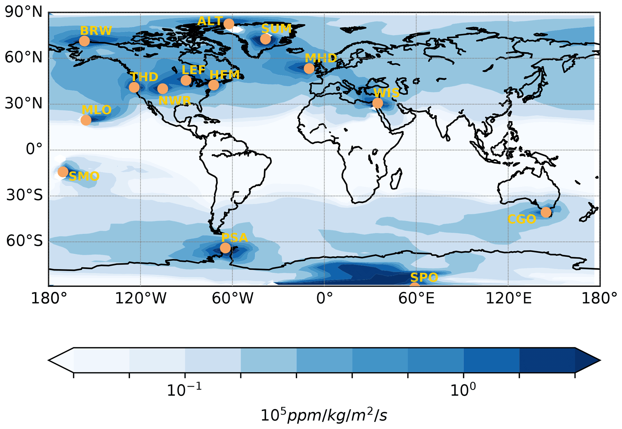
Figure 1Annual climatology of Jacobians computed by the adjoint of the LMDz model: map of the partial derivatives, in ppm kg−1 m−2 s−1, of a monthly mean concentration at all stations from the NOAA network with respect to CO2 surface fluxes in the 2 previous months. The yellow dots denote the location of the surface sites. The site KUM is not depicted as it has the same coordinates as MLO but at sea level.
Note that, if computed with respect to the COS fluxes, the annual climatology of the Jacobian shown in Fig. 1 would have the same spatial pattern but with a different unit given that the atmospheric transport is linear and there are no atmospheric chemical reactions.
2.2.2 Independent observations
An ensemble of independent observations – i.e., data that are not assimilated in LMDz – is used to evaluate the fluxes retrieved by our inverse system. We focus here on the observations used to evaluate the COS and the GPP fluxes.
The first observation programme is the HIAPER Pole-to-Pole Observations (HIPPO; Wofsy, 2011). HIPPO consisted of five aircraft transects of many trace gas measurements, including for COS and CO2, in the troposphere over the western Pacific: HIPPO 1 (January 2009), HIPPO 2 (November 2009), HIPPO 3 (March–April 2010), HIPPO 4 (June 2011) and HIPPO 5 (August 2011). The HIPPO measurements were made from flask and in situ measurements by NOAA and the University of Miami. They were rescaled to be consistent with the calibration scale used for the NOAA surface network results.
In order to assess the north–south latitudinal COS gradient over Japan, surface measurements for winter and summer 2019 at three sampling sites in Japan from Hattori et al. (2020) have been used as well: Miyakojima (24∘80′ N, 125∘27′ E), Yokohama (35∘51′ N, 139∘48′ E) and Otaru (43∘14′ N, 141∘16′ E). In winter, the Miyakojima site samples air masses strongly influenced by anthropogenic emissions from Chinese megacities including Beijing and Shanghai, while Yokohama and Otaru are only influenced by the northern periphery of China. During the summer, all sites mainly sample ocean air masses coming from southeastern Japan (Hattori et al., 2020).
The French sampling site, GIF (48∘42′ N–2∘08′ E), is located about 20 km to the southwest of Paris where ground-level COS has been monitored on a hourly basis since August 2014 (Belviso et al., 2020). According to the recent COS global gridded anthropogenic emission inventory of Zumkehr et al. (2018), the Paris region is an important source of COS (791 MgS yr−1, J. Stinecipher personal communication, November 2018) where its indirect emissions from the rayon industry largely overpass its direct emissions from the aluminium industry and traffic. These estimates have been challenged by Belviso et al. (2020). The locations of the HIPPO data, NOAA airborne profiles, and Japanese and GIF sites are depicted in Fig. 2.
The fourth observation programme is made of the satellite COS retrievals from MIPAS. The MIPAS spectrometer measured limb-emission spectra for several trace gases in the mid-infrared (Fischer et al., 2008) from the European Space Agency (ESA) Environmental Satellite (ENVISAT) between March 2002 and 2012. The IMK/IAA retrieval processor operated at KIT-IMK was used to calculate the COS profiles of data version V5R_OCS_221/222, which were used for this work (Glatthor et al., 2015, 2017). The number of vertical layers of the MIPAS retrievals is 60. Between altitudes of 7 and 25 km the accuracy of the COS profiles is around 50 ppt in the absence of clouds (in particular deep-convective ones) (Glatthor et al., 2015).
Last, the SIF satellite retrievals from the Global Ozone Monitoring Experiment-2 (GOME-2) make it possible to evaluate the seasonality of GPP inferred by inverse modelling for each PFT. SIF represents the amount of light reemitted by chlorophyll molecules as a byproduct of photosynthesis. Satellite-based SIF data are considered a proxy for the GPP of terrestrial ecosystems at large spatial–temporal scales (Frankenberg et al., 2011; Guanter et al., 2012; Zhang et al., 2016; Yang et al., 2015; Li et al., 2018). We use release number 28 of the NASA GOME-2 (Global Ozone Monitoring Experiment-2 on board the MetOp-A satellite) daily corrected SIF product (Joiner et al., 2013, 2016). The dataset is available at https://avdc.gsfc.nasa.gov/pub/data/satellite/MetOp/GOME_F/v28/ (last access: 7 February 2022). We used the monthly level 3 product gridded at a 0.5∘resolution between the years 2008 and 2019. This GOME-2 SIF product was shown to be very similar in terms of seasonality and magnitude (after spectral scaling) to the reference Orbiting Carbon Observatory (OCO-2, launched in 2014; Sun et al., 2018) data (Bacour et al., 2019). For each PFT, we average all the grid points within the LMDz grid points that have a fractional cover greater than 0.8. We lower this threshold to 0.3 for PFTs 7 (boreal broadleaved evergreen forest), 8 (boreal broadleaved summergreen forest), 9 (boreal needleleaf summergreen forest) and 15 (boreal C3 grass). The PFTs are further defined in Sect. 2.4.
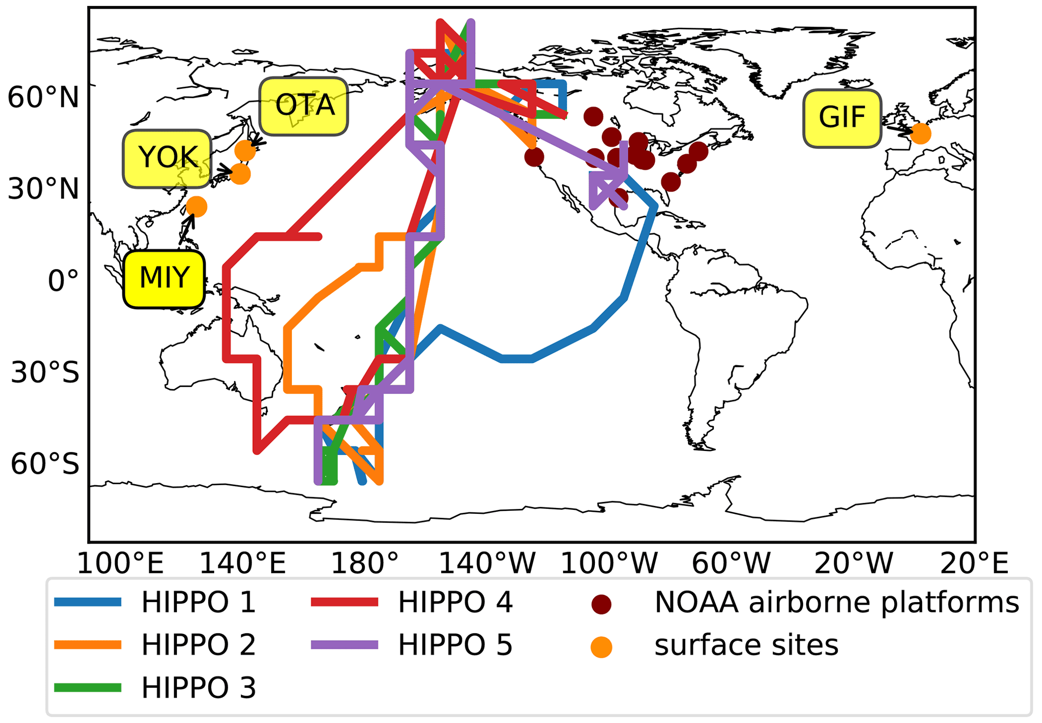
Figure 2Location of the HIPPO airborne measurements, NOAA airborne platforms and surface sites in Japan and France that are used as independent observations for evaluating the inverse results. The HIPPO measurements have been averaged into bins of 10∘ each. The NOAA airborne measurements are exploited in the Supplement.
2.2.3 Data sampling
For each species and each measurement, the simulated concentration fields were sampled at the LMDz 3D grid box closest to the observation location. As mentioned above, the observations at selected local times are assimilated as 8 d averages. For the independent observations, LMDz is sampled at the closest time from the observations. All observations are dry-air mole fractions calibrated relative to the compound World Meteorological Organization (WMO) mole fraction scale. Satellite retrievals are dry-mole fractions tuned by the data providers to the compound World Meteorological Organization (WMO) mole fraction scale. For comparison, the corresponding dry-air variables in the model simulations are used.
When comparing MIPAS data with LMDz simulations, the a priori and vertical sensitivity of the retrievals must be taken into account. For each MIPAS retrieval, the modelled COS profiles have been interpolated linearly to the MIPAS vertical resolution (60 layers) while ensuring the conservation of the column-average mixing ratio (Chevallier, 2015). They were then smoothed with the corresponding MIPAS averaging kernels.
The a priori profile for the COS retrievals is a zero profile (Glatthor et al., 2015); hence it did not need to be taken into account. As done in Glatthor et al. (2015), we focus here on the spatial distribution of the COS mixing ratio at the 250 hPa pressure level (still after convolution of the model with the averaging kernels) for the period 2008–2012. In order to dampen the random noise in the MIPAS observations, we aggregate the retrievals into latitude–longitude bins.
2.3 Inverse framework
Our inverse system seeks to estimate the amplitude of n sources or sinks of CO2 and COS gathered in a vector x by reducing the mismatch between the observed concentrations gathered in a vector yo and those simulated with the atmospheric transport model M forced by these sources and sinks. Together with an initial disaggregation operator (that converts the low-resolution control vector into gridded fluxes using gridded reference fluxes; see Sect. 2.5.1) and a sampling operator (see previous section), the linearized transport model M is part of the linear observation operator H that relates x and the model-equivalent CO2 and COS measurements y at the sites shown in Fig. 1:
In order to regularize the inverse problem corresponding to Eq. (1), we use a Bayesian framework involving an a priori control vector, xb, with its associated uncertainty statistics, summarized in covariance matrix B. Within the Gaussian assumption of the prior and observation errors, the solution of the inverse problem can be simply expressed by the following equation (see for instance Tarantola, 1989) for the posterior control vector xa and the uncertainty covariance matrix Pa:
with R the error covariance matrix of the observations, encompassing measurement errors and H errors. Within the Gaussian assumption with no bias for all errors, the above solution minimizes the cost function:
2.4 Gridded reference fluxes
In the following, we call “reference fluxes” the maps of CO2 and COS fluxes that are used in the observation operator, the control vector x being a low-resolution multiplier to these (see Sect. 2.5.1). For use at resolution , the maps of the following components of the CO2 and COS fluxes have been interpolated from their native resolution. All projections conserved mass.
2.4.1 CO2 fluxes
Our reference fluxes combine several information sources. Fossil fuel emissions are from the gridded fossil emission dataset GCP-GridFED (version 2019.1) (Jones et al., 2021). Biomass burning fluxes vary inter-annually and are described by the GFED 4.1s database (https://www.globalfiredata.org/data.html, last access: 7 February 2022). Monthly air–sea CO2 exchange is prescribed from the Copernicus Marine Environment Service database (Denvil-Sommer et al., 2019). The GPP and respiration fluxes have been simulated at a resolution of 0.5∘ in both longitude and latitude by the ORCHIDEE land surface model (Krinner et al., 2005). ORCHIDEE explicitly parameterizes the main processes influencing the water, carbon and energy balances at the interface between land surfaces and atmosphere. The vegetation is represented by 15 PFTs with a spatial distribution prescribed from the ESA Climate Change Initiative (CCI) land cover products (Poulter et al., 2015). The plant phenology is prognostic and PFT-specific. We used version 9 tuned for the CMIP6 exercise and forced by the global CRUJRA reanalysis at a global scale (https://sites.uea.ac.uk/cru/data/, last access: 7 February 2022) v1-v2, applying land-use change and realistic increase in CO2 atmospheric concentration. Emissions from the land use and wood harvest have been included beforehand in the respiration term. Biomass burning emissions are not taken into account in this respiration term from ORCHIDEE. The yearly global GPP from ORCHIDEE amounts to 126.7 GtC yr−1 during 2008–2019. This value is within the range of the GPP estimates (106–137 GtC yr−1) based on photosynthesis proxies (see Table S1) (Beer et al., 2009, 2010; Welp et al., 2011; Alemohammad et al., 2017; Jasechko, 2019; Jung et al., 2020; Ryu et al., 2011; Badgley et al., 2019; Stocker et al., 2019). The PFTs and their acronyms are defined in Appendix A. Note that GPP, respiration, COS vegetation and soil fluxes are null within PFT 1 (bare soil).
2.4.2 COS fluxes
The components of the COS budgets that are considered are biomass burning, soil emissions and uptake, anthropogenic emissions, plant uptake, oceanic emissions, and the atmospheric oxidation by the OH radical in the troposphere. Photolysis in the stratosphere, estimated at 30 GgS yr−1 in the LMDz atmospheric transport model (not shown), and volcano emissions, in the range 23–43 GgS yr−1, have been neglected (Whelan et al., 2018).
Kettle et al. (2002)Montzka et al. (2007)Suntharalingam et al. (2008)Berry et al. (2013a)Launois et al. (2015b)Ma et al. (2021)Table 1Overview of the global budget of COS. Units are GgS yr−1.
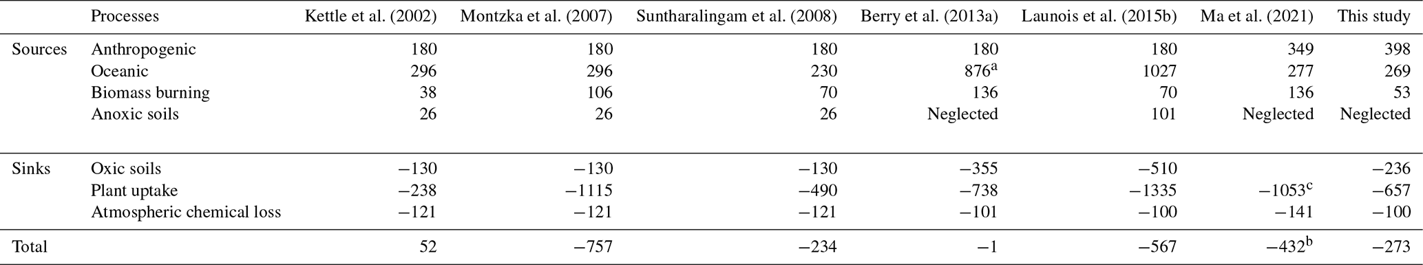
a In order to provide a balanced COS budget, the oceanic emissions from Kettle et al. (2002) have been increased by 600 GgS yr−1. b This unknown source has been optimized using a global four-dimensional variational data assimilation system. c This number corresponds to the soil and plant uptake combined.
2.4.3 Soil
Reference air–surface exchanges from oxic soils have been simulated by the steady-state analytical model of Ogée et al. (2016) implemented in the ORCHIDEE land surface model with the Zobler soil classification at 0.5∘ in both longitudes and latitudes (Abadie et al., 2021). This model is built on the assumptions that the soil–atmosphere exchanges are governed by three processes, namely diffusion through the soil column, production and irreversible uptake via hydrolysis. The COS uptake reflects, for the most part, the activity of CA, ubiquitous in soil microorganisms, which efficiently converts COS into H2S and CO2, similarly to what happens in plants. The CA activity is represented by the CA enhancement factor or fCA, which is PFT-specific and has been calibrated against measurements performed by Meredith et al. (2018) on different biomes in the laboratory. The production term simulates the COS abiotic production from soils via the Whelan et al. (2016) model. Its exponential increase with temperature decreases the net soil uptake over the tropics and in mid-latitudes in summer. The soil model has been shown to be in better agreement with measurements than the Berry et al. (2013a) model used in previous top-down studies. As for the contribution of anoxic soils (Whelan et al., 2013), we have not taken them into account in the absence of reliable emission maps (Whelan et al., 2018).
2.4.4 Plant uptake
We chose the empirical formulation of the COS uptake by leaves from Sandoval-Soto et al. (2005) given by the linear relationship
In this equation, FCOS and GPP are the COS uptake and the CO2 uptake (both in ppm m−2 s−1), respectively, and [COS] and [CO2] being the ambient air concentrations of COS and CO2. vCOS and are the COS and CO2 leaf uptake velocities. The ratio of uptake velocities of COS compared to CO2 is defined as the LRU:
We use a zero-order LRU approach (i.e., with no interaction between vegetation and COS mixing ratio), given the complexity of an order approach (i.e., a coupled atmospheric COS concentration – COS flux calculation). To address this shortcoming, we use the time-evolving hemispheric means of the COS and CO2 atmospheric concentrations, NHmean and NSmean as done in Montzka et al. (2007). They are computed from monthly means at selected stations or groups of stations weighted by the cosine of latitude of atmospheric boxes encompassing different site groupings in this way.
We have only made a distinction between C4 (LRU = 1.21) and C3 plants (LRU = 1.68) and disregarded the dependence on light and water vapour deficit that was observed at both leaf (Stimler et al., 2010) and ecosystem scales (Maseyk et al., 2014; Commane et al., 2015; Kooijmans et al., 2019). Our LRU set is derived from Whelan et al. (2018) and uses, for C3 plants, the median value of 53 LRU data and, for C4 plants, the median value of 4 LRU data. This simplification is supported by Hilton et al. (2017) and Campbell et al. (2017), who showed that the uncertainty on the LRU parameter is of a second-order importance compared to the uncertainties on the GPP and the other COS fluxes. Moreover, Maignan et al. (2020) showed that using a mechanistic model or its LRU equivalent model (i.e., with a constant LRU per PFT in ORCHIDEE LSM) for the plant uptake leads to similar results when transporting the COS fluxes with LMDz and comparing the COS concentrations at stations of the NOAA network. A physical reason making the LRU simplification acceptable is that the observation sites sample plant sink signals from multiple parts of the day. We have not taken into account the epyphites which can both emit and absorb COS depending on environmental conditions (Kuhn and Kesselmeier, 2000; Rastogi et al., 2018).
2.4.5 Anthropogenic fluxes
For anthropogenic fluxes, we use the inventory of Zumkehr et al. (2018) for the period 1980–2012 that corresponds to a global source of 398 GgS yr−1 (range of 223–586 GgS yr−1) for the period 2009–2019. Emissions after 2012 are taken from the year 2012. The inventory accounts for direct COS emissions and indirect emissions through the oxidation of CS2 into the atmosphere. The considered emissions are, in order of importance, emissions from the rayon (staple and yarn) industry, residential coal, pigments, aluminium melting, agricultural chemicals and tires. Compared to Kettle et al. (2002), the majority of the sources has shifted over time from the US to China which encompasses now 45 % of the total emissions.
2.4.6 Ocean
COS is directly emitted by the ocean in places where the sea water is saturated in COS. Emissions typically happen in summer in high latitudes. COS is also indirectly emitted through the oxidation of DMS and CS2 in the atmosphere, which are both produced in seawater. We use the indirect and direct COS emissions from Lennartz et al. (2017, 2020a), whose total emissions account for 285 GgS yr−1. In these, direct emissions via CS2, indirect emissions via CS2 and indirect emissions via DMS from the global ocean account for 130±80, 74±120 and 65–110 GgS yr−1. These emissions have all been computed using box models calibrated with ship-borne measurements made in different parts of the globe (Lennartz et al., 2017, 2020a). The DMS emissions are taken from the Lana et al. (2011) climatology. The latitudinal distributions of each of the three terms of the oceanic emissions are depicted in Fig. 3.
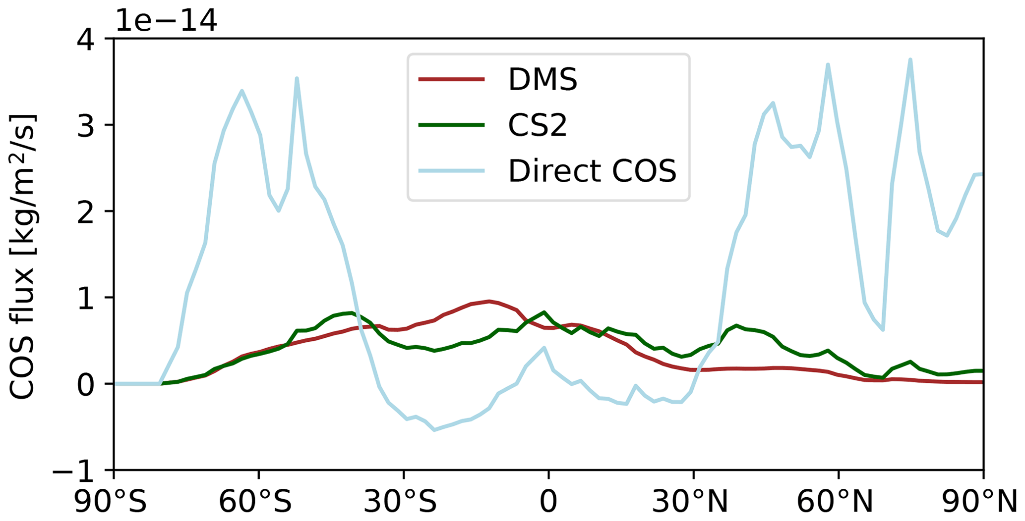
Figure 3Zonal mean distribution of the prior oceanic fluxes as a function of latitude averaged over the year 2010. The direct COS emissions are shown in blue whereas the indirect COS emissions through DMS (CS2) are depicted in brown (green).
We have not considered DMS and CS2 as separate tracers as done in Ma et al. (2021). CS2 has a lifetime estimated between 4 d (Khan et al., 2017) and 12 d (Khalil and Rasmussen, 1984), and DMS has a lifetime of 1.2 d. For the sake of simplicity, the oxidation of CS2 and DMS by OH has been assumed to happen instantly in the atmosphere.
2.4.7 Biomass burning
We use the inventory emissions from Stinecipher et al. (2019) with a global estimate of 60±37 GgS yr−1 for the period 1997–2016. These authors used CO as a reference species to compute the COS biomass burning emissions. To do that, they combined emission factors of COS to CO from the literature and applied them to the CO emissions. These CO emissions were computed beforehand from the GFED Global Fire Emissions Database (GFED version 4, https://www.globalfiredata.org/, last access: 7 February 2022). The resulting biomass emissions are classified into four categories: savanna and grassland, boreal forests, temperate forests, tropical deforestation and degradation, peatland fires, and agricultural waste burning. The savanna was shown to be the largest contributor to the global biomass burning emissions and therefore to the overall uncertainty. These new estimates are lower than the previous estimate of open burning emissions. The latter were also positively biased by a strong emission factor derived from measurements over the peatlands. Moreover, their weak inter-annual variability was shown to better reproduce the annual trend in atmospheric concentration at the Jungfraujoch station, the long-term trend being primarily driven by changes in anthropogenic activity (Zumkehr et al., 2017). It should also be noted that, compared to the Kettle et al. (2002) inventory, the inventory emissions from Stinecipher et al. (2019) do not include biomass burning sources from agriculture residues and biofuels. The latter were estimated to be about 3 times as large as open burning emissions (Campbell et al., 2015).
2.4.8 OH sink
Since the highest reaction rate is close to the surface (Kettle et al., 2002), we represent the OH sink by a surface flux. As done in Launois et al. (2015b), we take the spatial patterns of monthly maps of the OH radical concentrations, and we distribute a total annual tropospheric sink of 100 GgS yr−1 both horizontally and temporally, suggested by previous estimates (Kettle et al., 2002; Berry et al., 2013b). We use monthly maps of OH radical concentrations from an update of Hauglustaine et al. (2004).
2.5 Inversion configuration
2.5.1 Control vector
Our inversion window covers 12 years. The spatiotemporal resolution of the control vector x over this period represents a compromise between the assumed resolution of the errors of the reference fluxes, the expected resolution of the flux increments that can be inferred by the sparse site distribution (see Fig. 1) and considerations on computing time. Typically, a large control vector (i.e., many controlled regions and types of emission) may represent the complexity of reality better than a small control vector (i.e., few regions and emission processes) but also increases the inversion calculation load without always improving inversion skill, given the scarce and uneven observation network. The variables in the control vector are therefore all multipliers of the above-described gridded reference fluxes, as described as follows, rather than grid-point fluxes themselves. The choice of multipliers rather than increments implies that the initial sub-control-scale patterns are kept. The prior control vector xb is simply a vector of values of 1.
We control COS oceanic fluxes in three latitudinal bands: the tropics, the northern latitudes and the southern latitudes. This separation allows the inverse system to modify the latitudinal distribution of the reference emissions, which remains subject to large uncertainties, while preserving the prior longitudinal patterns. This amounts to saying that the coastal sites located in the Northern Hemisphere constrain the total oceanic emissions over the whole Northern Hemisphere above 30∘ N. The ocean emissions are only modified within each of the three latitudinal bands by a single specific factor. Because the role of indirect COS emissions through DMS is still a matter of debate (Von Hobe, M., personal communication, 2020), we take all ocean emissions as a whole. On the continents, for respiration, GPP and soil fluxes, we distinguish the two hemispheres for eight of the 15 PFTs which are present in both (4, 5, 6, 10, 11, 12, 13; see Appendix A) to take into account the different seasonality. For the anthropogenic COS emissions, we control a single annual emission coefficient and rely on the reference distribution of sources between Europe, Asia and America: the lack of observations in the Asia–Pacific region does not allow us to separately optimize Asian emissions. All parameters are optimized on a monthly scale with the exception of anthropogenic emissions, which are assumed to be constant throughout the year.
For the CO2, we neglect the uncertainty on the oceanic, fire and anthropogenic CO2 emissions compared to that of the sum of the respiration and GPP. The parameters of the control vector are described in Table 2.
Table 2Controlled variables for 1 year. The size of the control vector is equal to 149 630 for the inversion period 2008–2019.
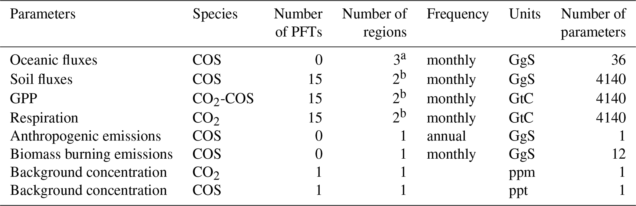
a The ocean flux is divided into three regions: 30∘ N–90∘ N, 90∘ S–30∘ S, 30∘ S–30∘ N. b GPP, respiration and soil fluxes of PFTs 4, 5, 6, 10, 11, 12 and 13 are divided into two hemispheres: 0∘ N–90∘ N, 0∘ S–90∘ S.
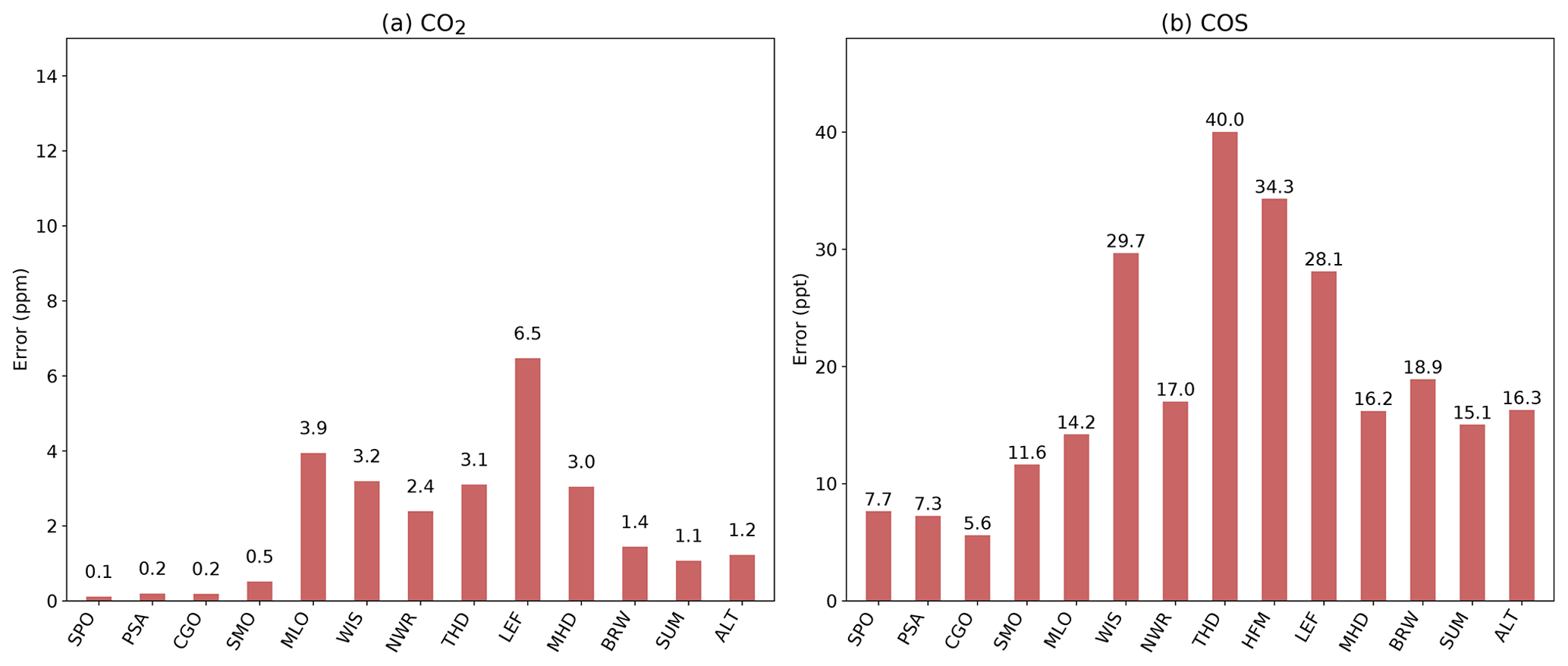
Figure 4Assigned error standard deviations for each station and for (a) CO2 and (b) COS. Stations are ordered from the South Pole (on the left) to the North Pole (on the right).
2.5.2 Prior and observation error covariance matrices
Observation errors are defined with respect to the observation operator H and are actually dominated by the errors of H. As explained in Sect. 2.3, H is made of a disaggregation operator, a transport model and a sampling operator. For the transport model error statistics, we follow the detail of the approach described by Chevallier et al. (2010), who used the statistics of the difference between the raw times series and the corresponding smooth curve as a proxy. This approach yields one error standard deviation per station. The procedure to derive the smooth curve is explained in Sect. 2.6. We doubled the resulting standard deviation at each station in order to account for the error induced by the disaggregation operator. The error is likely larger at stations NWR, LEF, HFM and WIS partly because of the larger influence of nearby fluxes, and we have applied an additional twofold factor there. For instance, LEF is located in the Midwestern states, a region contributing half of the summer carbon uptake in North America (Sweeney et al., 2015). Similarly, the standard deviation is also multiplied by 2 at the station SMO to the challenging representation of sub-grid-scale transport by deep convective clouds in the tropics. The resulting observation error standard deviation at each stations is shown in Fig. 5.
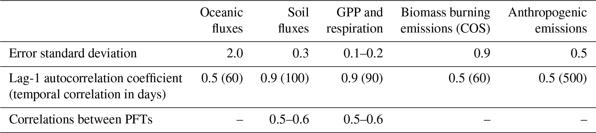
Table 3Description of the prior error covariance matrix. Since the control vector is made of low-resolution multipliers to reference maps, the standard deviations are fractions of the reference values. The lag-1 autocorrelation coefficients are the correlations assigned between two consecutive time steps for each controlled variable, the time step being defined in Table 2.
Our prior error covariance matrix B (that applies to xb, a vector of values of 1; see Sect. 2.5.1) is described in Table 3. Although the large number of parameters offers very diverse possibilities for the definition of the error covariance matrix, we present only one scenario that is optimal in terms of fit to observations among those that we find compatible with our knowledge of the errors of the reference maps.
-
GPP and respiration. The monthly-mean GPP from ORCHIDEE within each of the PFTs agrees with site-level GPP estimates from eddy covariance measurements in the range of 20 % (not shown). For PFT 2 (tropical broadleaved evergreen forests), we reduce the 1σ uncertainty to 10 %, a more realistic value given the large gross fluxes over the tropics. We introduce some non-diagonal terms in the prior error covariance matrix to represent likely error correlations between PFTs given that they share the same equations in the ORCHIDEE model for most processes. Thus, the errors in the PFTs mainly located over the high latitudes (PFTs 7, 8, 9, 15), the mid-latitudes (PFTs 4, 5, 6, 10) and the tropics (PFTs 2, 3, 11, 14; see Appendix A for a description of the PFTs) are set to be correlated with a factor of 0.6 (high latitudes), 0.5 (mid-latitudes) and 0.6 (the tropics), respectively. Thus, over the high latitudes, the PFTs 7, 8, 9 and 15 are correlated with a factor of 0.6. We further introduce temporal correlations for GPP and respiration. At the first order, we expect that the errors associated with the monthly GPP simulated by ORCHIDEE are positively correlated because (i) errors in the structure of the ORCHIDEE model likely lead to positively correlated flux errors, and (ii) parametric errors will also provide similar correlations. However, errors in the meteorological forcing may de-correlate the gross flux errors, which could justify an exponential decay as a function of time. The memory effect linked for example to soil moisture (and thus precipitation) may also induce error correlation (Stocker et al., 2019). For the annual global GPP, this set-up leads to a 1σ uncertainty of 5 GtC yr−1 for a reference value here of 125 GtC yr−1: this uncertainty may look small compared with the range of GPP estimates found in the literature (see Table S1) but is in agreement with the most recent estimation of 125±5.2 GtC yr−1 from Stocker et al. (2019). The same set-up has been chosen for plant respiration. There are error correlations between GPP and respiration, but these are neglected in this study.
-
Oceanic emissions. Our resulting 1σ uncertainty of 350 GgS yr−1 for the globe and the year, given a reference value of 271 GgS yr−1 (see Fig. 4), is consistent with Lennartz et al. (2017, 2019, 2020a), who estimated the ocean emissions between 120–600 GgS yr−1 .
-
Anthropogenic emissions. Our correlation length of 500 d damps interannual variations, consistent with Zumkehr et al. (2018), who found that they do not vary by more than 5 % from one year to the next. The resulting 1σ uncertainty of 197 GgS yr−1 for the globe and the year, given a reference value of 370 GgS yr−1 (see Fig. 4), is consistent with the estimation of 223–586 GgS yr−1 given by Zumkehr et al. (2018).
-
Soil fluxes. Our choice of a standard deviation of 30 % is rather arbitrary given the lack of measurements to evaluate the reference soil flux within each PFT. We also assign a large autocorrelation length (100 d) to damp month-to-month variations, consistent with local measurements made at Harvard and Gif-sur-Yvette (Belviso et al., 2020; Commane et al., 2015).
2.6 Post-processing of the CO2 and COS simulations and measurements
The seasonal cycle is derived from the surface data using the CCGVU curve-fitting procedure developed by Thoning et al. (1989) (http://www.esrl.noaa.gov/gmd/ccgg/mbl/crvfit/crvfit.html, last access: 7 February 2022). The procedure estimates a smooth function by fitting the time series to a first-order polynomial equation for the growth rate combined with a two-harmonic function for the annual cycle and a low-pass filter with 80 and 667 d as short-term and long-term cutoff values, respectively.
2.7 Metrics
The simulated atmospheric concentrations (for CO2 or COS here) are evaluated against measurements using the root mean square error, RMSE, defined as
where N is the number of considered observations, CObs (n) is the nth observed concentrations and CMod(n) is the nth modelled concentration. The unit of RMSE is in ppm (ppt) for CO2 (COS).
The global χ2 is equal to twice the cost function J(x) at its minimum (see Eq. 3 for the general definition of the cost function):
The variables are defined in Sect. 2.3. This metric allows us to check the consistency of the error covariance matrices. The χ2 follows the so-called chi-square law, with the number of degrees of freedom equal to the number of observations (Nobs) (as in our case the observation error covariance matrix is diagonal). The ratio (normalized χ2) should therefore be close to 1. This means that the residuals between observed and simulated concentrations should be aligned with the assigned measurement errors, and the residuals should be distributed as a Gaussian around the observed values. A value larger (smaller) than 1 may indicate that the assigned uncertainties (of the measurements and/or from the a priori fluxes) are too small (too large). However, tuning the prior and observation covariance matrices with the sole normalized χ2 may actually be misleading since the matrices involve many variables (including off-diagonal elements) that may play compensating roles in the χ2 (Chevallier, 2007).
The χ2 per station, , represents the contribution of each site to the first term of the global χ2. For a station i, the metric is defined as
with Hxi)T and being the simulated and observed concentrations at station i. This value, divided by Nobs (normalized ), should ideally be close to 1. A value larger (smaller) than 1 may indicate that the assigned uncertainties of the measurements at this station are too small (too large).
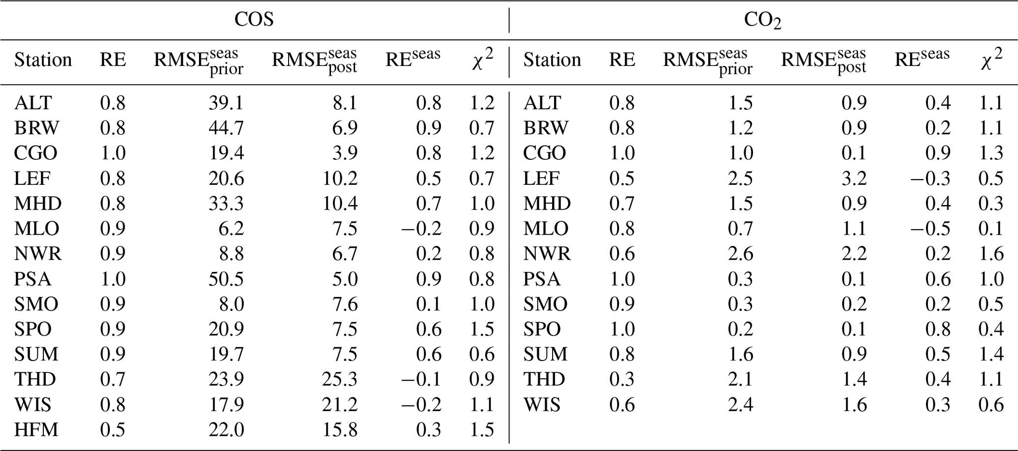
Table 4Column “RE” presents the fractional reduction of the model vs. assimilated measurement RMSE . Column “” presents the RMSE of the a priori detrended time series compared to the assimilated measurement time series. Column “” presents the RMSE of the a posteriori detrended time series. Column “REseas” presents the reduction of uncertainties using the RMSE metrics applied to the detrended time series . Column “χ2” presents the reduced chi-squared statistics (without unit) for each station. The detrended curves have been filtered to remove the synoptic variability (see Sect. 2.6). The RMSE is in ppm (ppt) for CO2 (COS). All statistics are for the period 2009–2019.
3.1 Comparison to the assimilated surface measurements
Table 4 shows the error reduction achieved by the inversion in terms of RMSE between the simulated and the observed concentrations. As expected, the inverse system has reduced the observation–model mismatch by about 85 % at most stations. Of interest in Table 4 is also the error reduction for the detrended smooth curves in which only seasonal variations are retained. It is indeed important to accurately represent the large COS and CO2 surface depletion in spring as it mainly reflects the amplitude of the GPP over the continents. The seasonal error reduction is usually smaller than the overall error reduction: the COS inversion mainly corrects the negative tendency in COS mixing ratio arisen from the unbalanced prior budget. For instance at MLO between 2008 and 2011, the tendency of the CO2 (COS) concentrations a priori is 3.9 ppm yr−1 (−57 ppt yr−1) against 2.0 ppm yr−1 (1.4 ppt yr−1) in the observations. Yet, the inversion has reduced the seasonal misfits to observations at most sites except at LEF and MLO for CO2 and MLO, THD and WIS for COS. At the northernmost sites (ALT, BRW, SUM, MHD), the error reduction exceeds 50 % for both compounds. Despite some improvements, the inversion still struggles to represent the seasonal cycle of the COS measurements at the sites WIS, HFM and THD for which the RMSE remains greater than 15 ppt. THD is a coastal station which suffers from the influence of fluxes nearby (Riley et al., 2005). For this reason, modelling the variability of its CO2 and COS mixing ratio has been shown to be particularly challenging (Ma et al., 2021). The inverse system also struggles to match CO2 measurements at the sites WIS, NWR and LEF with a seasonal RMSE greater than 1.5 ppm.
The consistency of the estimate with the measurement errors and the a priori flux errors assumed is analysed first with the global normalized chi-squared statistic (see Eq. 9). This metric should ideally be close to 1. In our case, the normalized χ2 equals 1.04, a value consistent with a fair configuration. The relative contribution of the measurement term (first term of Eq. 9) to the total χ2 (Eq. 9 or cost function at its minimum) is much larger than that of the flux term (80 % versus 20 % on average), suggesting that the a priori constraint is rather loose.
In addition to the global consistency between data errors and a priori flux errors, the validity of the relative weights (inverse of the squared data error) assumed for the individual measurement residuals (i.e., at each station) is assessed (see Eq. 10). To this end, Table 4 shows the χ2 per station. The value is less than 1 for 7 stations out of 15 for both compounds, meaning that the residuals are within the range of the assigned observation uncertainty. Among the stations with χ2 values greater than 1, HFM stands out, and likely we assigned too small uncertainties to this station.
In order to better visualize the improvement on the seasonal cycle, we compare in Fig. 5 the simulated a priori and a posteriori concentrations against observations at three sites: BRW, NWR and LEF. These time series have been detrended beforehand to retain the seasonal cycle. At BRW, the inversion has corrected the too low seasonal amplitude and the phase lag in the a priori concentrations within the range of observation uncertainties. At LEF, the a priori concentrations were already in good agreement with the observations, and the inversion has not improved the simulated concentrations much. However, at NWR, the inversion struggles to correct the advanced phase, especially in the CO2 simulations, consistent with a χ2 greater than 1. One likely explanation is that our biome-scaling approach with one coefficient per PFT is too coarse to correct the spatial distribution of the prior fluxes, especially between relatively close sites such as NWR and LEF. The latter are more prone to be influenced by local fluxes than ocean stations such as MHD for example.
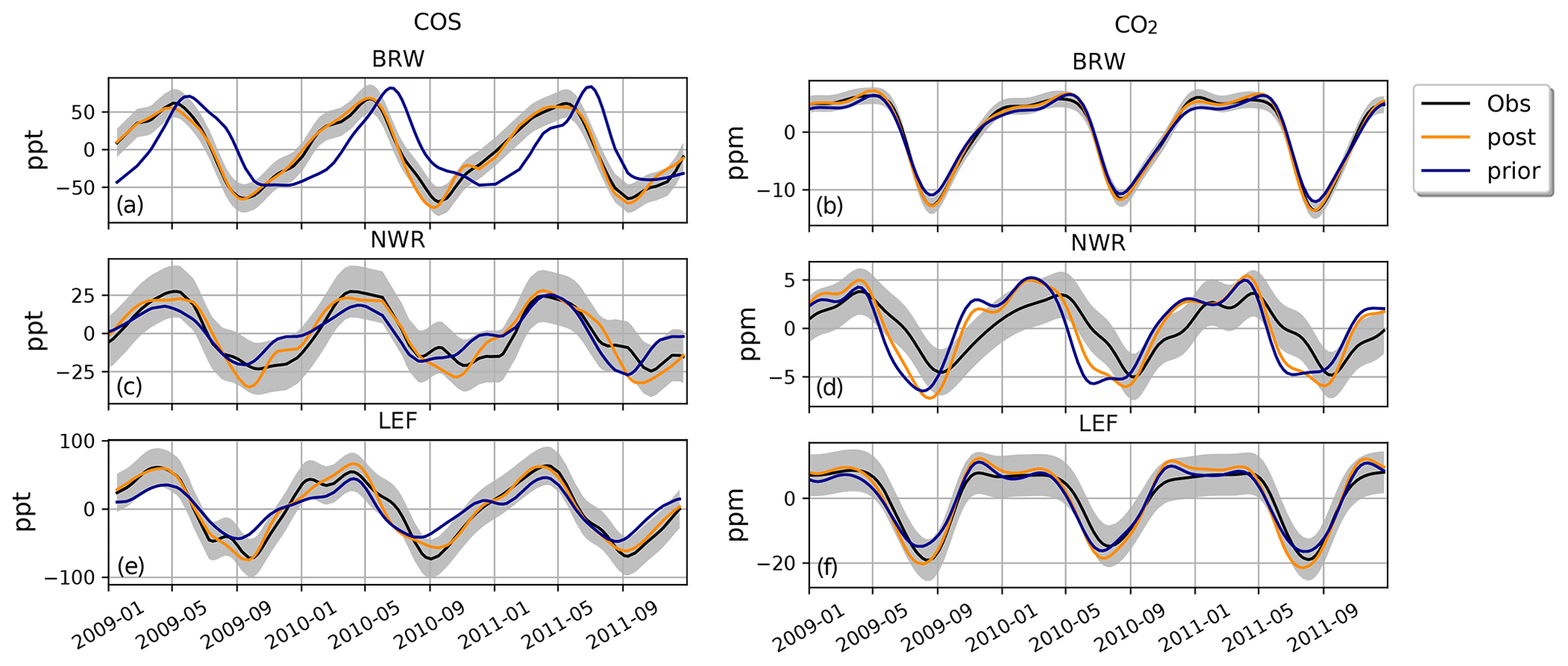
Figure 5Detrended temporal evolutions of simulated and observed CO2 and COS concentrations at three selected sites, for the a priori and a posteriori fluxes, simulated between 2009 and 2011. (a, b) Barrow station (BRW, Alaska, USA), (c, d) Niwot Ridge (NWR, USA) and (e, f) Park Falls (LEF, USA). The curves have been detrended beforehand and filtered to remove the synoptic variability (see Sect. 2.6). The grey bar represents the 1σ error bar of the observations.
3.2 Optimized fluxes
Table 5 summarizes our top-down assessment of the COS and the CO2 budgets. The inversion doubled the COS oceanic emissions to 530 GgS yr−1. Given the missing source in the reference fluxes, the ocean dominance in the measurement footprints and the efficient reduction of the global error by 90 %, the increase in oceanic emissions is an expected behaviour of the Bayesian inverse system. In contrast, the inversion marginally decreased the total soil and vegetation absorption likely due to the seasonal constraints. Following a decrease of 7 GtC yr−1 in the GPP to match the COS constraint, the respiration has decreased by 10 GtC yr−1 in order to keep a land carbon sink in agreement with the global atmospheric CO2 budget. Thus, on a global scale, the inversion seems to have corrected the overestimated prior atmospheric trend by a larger decrease in respiration than in GPP. All residuals between the total prior and the posterior fluxes are within the assumed 1σ range of the prior uncertainty, except for respiration, where the increment is twice as large as the standard deviation. The residuals are even much smaller than the prior standard deviation for the anthropogenic and the biomass burning emissions, suggesting that we could have narrowed the initial errors for those components.
The total oceanic COS emission remains lower than previous top-down studies using different configurations and observations, which instead estimated an oceanic source between 700 and 1000 GgS yr−1 (Berry et al., 2013a; Kuai et al., 2015a; Launois et al., 2015b). Several reasons could explain these differences. Firstly, the Zumkehr et al. (2018) anthropogenic emissions are much higher than the Kettle et al. (2002) one used in these previous studies. Secondly, we assimilated continental surface measurements from the NOAA network through the whole years of 2008–2019 while Kuai et al. (2015a) assimilated a single month of satellite retrievals over the tropical oceans. Finally, the prior biospheric and oceanic fluxes used, especially over the tropical domain, a region that is poorly constrained in the inversion, could explain the differences with the previous COS budgets. Launois et al. (2015b) noticed a dependence between the magnitude of the optimized ocean source and the prior vegetation uptake. The larger biospheric sink used in Launois et al. (2015b) and Berry et al. (2013a) requires a larger oceanic source over the tropics to close the COS budget. This is particularly true for Berry et al. (2013a), who used a fixed large biospheric sink of 1100 GgS yr−1.
Table 5Prior and posterior total fluxes and their associated 1σ uncertainty as part of the COS (top) and the CO2 (bottom) budgets. The mean magnitude of the different types of fluxes is given for the period 2009–2019. The vegetation sink is computed from the vegetation uptake (table on the right) using the LRU relationship described in Eq. (4). The components of the CO2 and COS budgets, as written here, have been obtained by adding all the related optimized parameters (see Table 2 for a description of the parameters). The flux convention is positive upwards (from the surface to the atmosphere). For a given component, the associated uncertainty is the root mean square of the sum of all the posterior error covariance terms related to the component divided by the number of years (11 here).
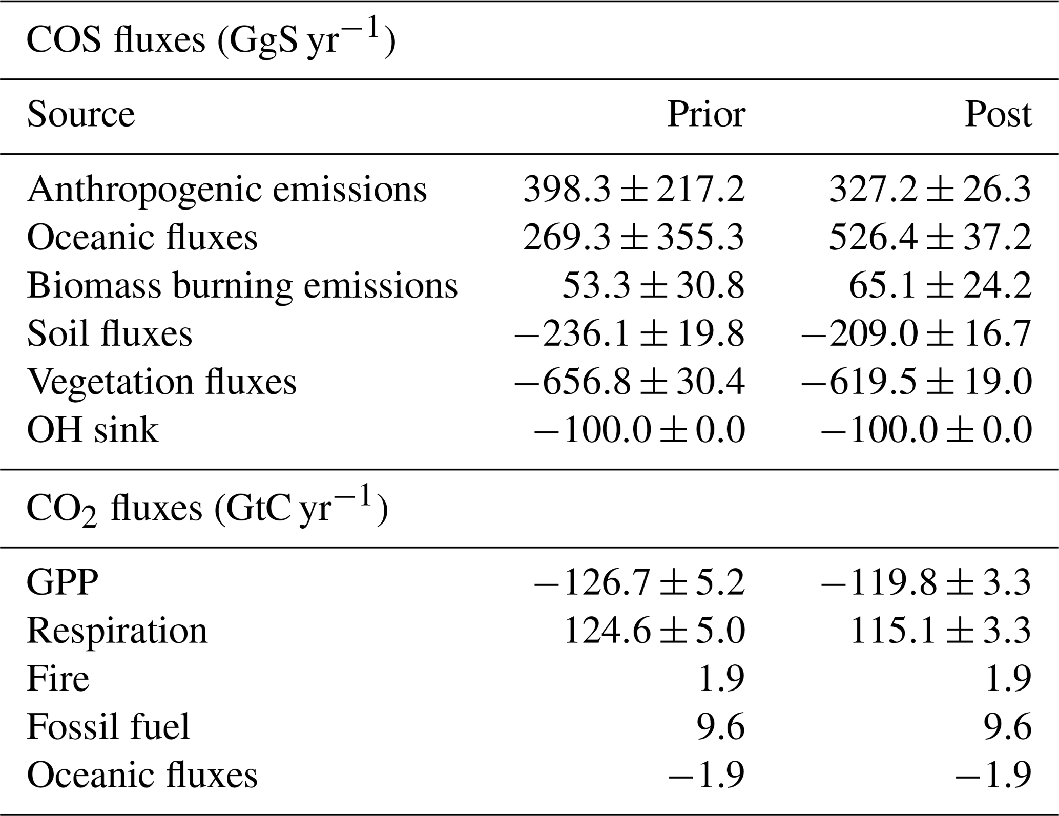
Figure 6 represents the zonal mean of the prior and posterior oceanic and continental COS fluxes as a function of latitude. The inversion increased ocean fluxes over the tropics while decreasing them in the high latitudes. This behaviour was already noticed by Berry et al. (2013a), who used a different inverse system and the Kettle et al. (2002) oceanic flux as a prior. Over the tropics, COS and CS2 measurements in sea waters do not support this increase as already mentioned in the introduction (Lennartz et al., 2017, 2020a). However, COS emissions through DMS oxidation in a pristine marine environment could play a role in sustaining this tropical source. Over the northern and southern oceans, high emissions in our reference oceanic flux from Lennartz et al. (2017) mainly arise from the direct oceanic emissions (see Fig. 3). The latter could be overestimated: the COS concentrations simulated by the ocean box model are higher than most of the measurements made in sea waters sampled over different parts of the globe (Lennartz et al., 2017). This remark supports the inversion decrease in the oceanic emissions over the mid-latitudes and high latitudes. The decrease beyond 50∘ towards the poles also reflects a seasonal cycle in COS sea water concentrations of a much lower amplitude than the one in atmospheric COS in the marine boundary layer (Lennartz et al., 2020b). This strong marine seasonal cycle is not attenuated enough by mixing processes within the boundary layer, and the inversion weakened the oceanic release to match the seasonal cycle in atmospheric COS concentrations at BRW and ALT. In particular, the emissions in the northern high latitudes have been suppressed in summer to correct the late peak in the time series at BRW in Fig. 5. While oceanic emissions decrease in the high latitudes, the terrestrial sink tends to increase. The change in terrestrial sink is mainly attributed to vegetation (see Fig. S4). The change in soil fluxes goes in the same direction as the change in COS vegetation uptake.
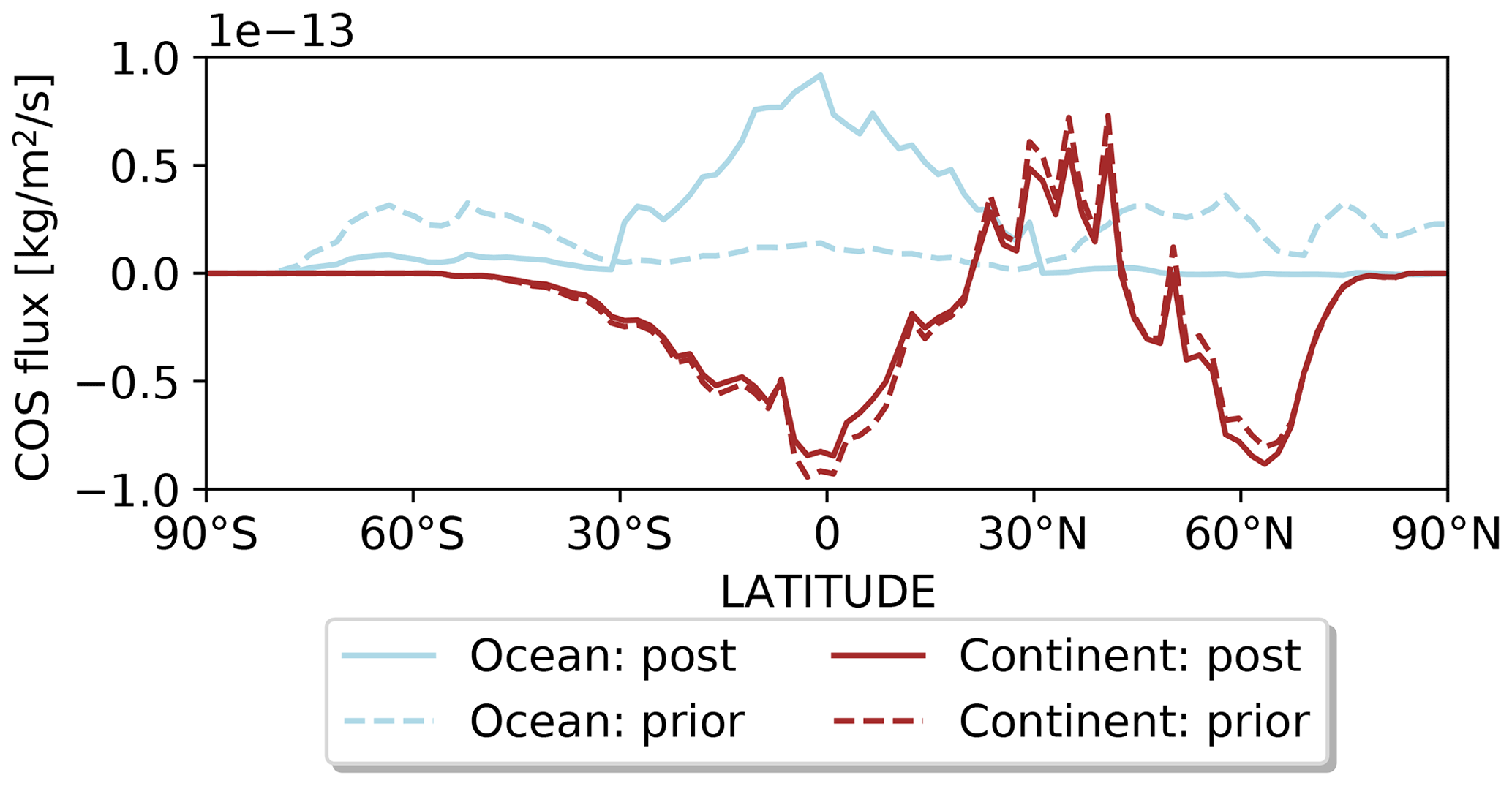
Figure 6Latitudinal distribution of the prior (dashed line) and posterior fluxes (full line) for the continental (brown) and oceanic components (blue) of the COS budget. The fluxes have been averaged over the years 2009–2019.
Regarding the impact on the CO2 budget, Fig. 7 shows the latitudinal distribution of the net CO2 vegetation fluxes defined as the sum of respiration and GPP before and after inversion. The inversion has increased the net vegetation absorption above 50∘ N almost 3-fold. This response is a common feature of the current inverse systems, which, by assimilating CO2 measurements only into an atmospheric transport model, infer a higher net vegetation sink in the high latitudes than land-surface models. Indeed, in Fig. 8 of Friedlingstein et al. (2020), the net land sink (above 30∘) calculated as the average of 17 process models is between 0.5 and 1.5 GtC yr−1 whereas the flux calculated from six inverse systems is between 1 and 2.5 GtC yr−1 averaged over the last 10 years. More specifically, Fig. 8 illustrates how the inversion changes the seasonal cycle of GPP and respiration within each of the 15 PFTs of the ORCHIDEE model. The changes in the global total per PFT are shown separately in the Supplement (see Fig. S4). In the tropics within PFTs 2 and 3 (tropical broadleaved evergreen and raingreen forests; see Appendix A), the inversion decreased GPP by about 4 GtC yr−1 whereas respiration lost 1 GtC yr−1, leading to a small source of CO2. In the mid-latitudes (PFTs 4, 5 and 10, Appendix A), the inversion weakened GPP and respiration by 5 and 2 GtC yr−1, respectively. The second salient change is an increase in CO2 absorption within the high latitudes covered by PFTs 7, 8, 9 and 10 (see Appendix A). Indeed, GPP increased by almost 2 GtC yr−1 while respiration only decreased by 0.2 GtC yr−1 in total. The increased GPP over the boreal latitudes explains the larger seasonal cycle of the a posteriori COS and CO2 concentrations at sites BRW and ALT. The comparison of GPP and respiration from ORCHIDEE against eddy covariance measurements at several sites around the globe pointed at an underestimation of these components, consistent with our inversion results (not shown). A complete validation of this ORCHIDEE version will be the topic of a future publication.
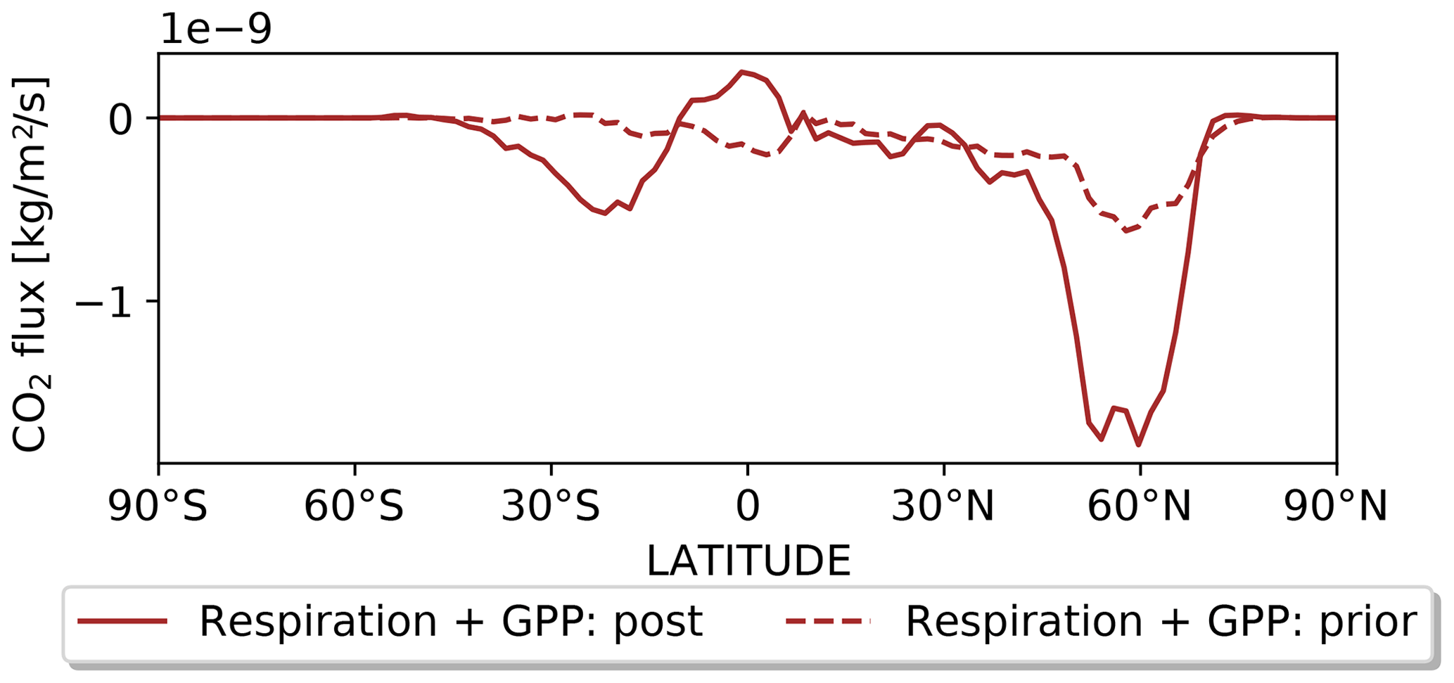
Figure 7Latitudinal distribution of the prior (dashed line) and posterior net CO2 fluxes from the terrestrial vegetation (full line). Vegetation fluxes are the sum of GPP and respiration fluxes. The fluxes have been averaged for the years 2009–2019.
3.3 Comparison with independent observations
3.3.1 Evaluating the seasonal cycle with SIF data
In order to assess the realism of the a posteriori GPP, its seasonal cycle is compared with the seasonal cycle of the GOME-2 SIF product. Although the ecosystem-dependent bias in the SIF products makes a direct comparison with GPP impossible, SIF has been recognized as a good indicator of the temporal dynamics in GPP. At the ecosystem scale, SIF is anti-correlated with the GPP: a maximum in SIF corresponds with a minimum in GPP. Figure 8 superimposed the maximum of the SIF on the GPP seasonal cycle. The normalized SIF seasonal cycle is further shown in Fig. S6. Ideally, the maximum coincides with the minimum of the GPP seasonal cycle. Overall, the inversion has not altered the timing of the COS seasonal depletion. The optimized seasonal cycle disagrees with the SIF satellite retrievals within PFT 2 (tropical broadleaved evergreen), PFT 3 (tropical boreal raingreen forest) and PFT 14 (tropical C3 grass), questioning the realism of a weaker CO2 and COS absorption over the tropics. Within PFT 2, the inversion tends to produce a seasonal signal in opposite phase with SIF. In the mid-latitudes, the seasonal phase of GPP is slightly degraded within PFT 4 (temperate needleleaved evergreen forest) while it is improved within PFT 12 (C3 agricultural land). In the high latitudes, the phase of the seasonal cycle, which was in quite good agreement with the SIF in the GPP a priori, has not been altered by the inversion. To conclude, the atmospheric inversion does not lead to a clear improvement in the representation of the GPP seasonal cycle.
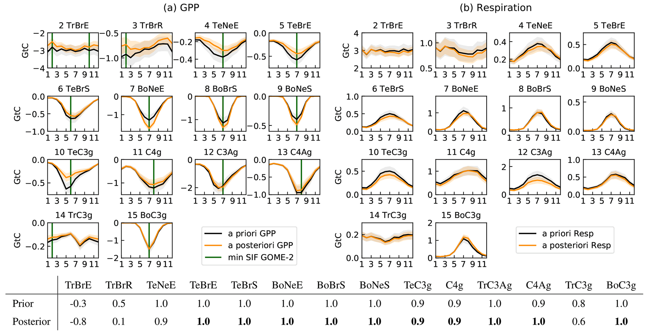
Figure 8Mean seasonal cycle of the total prior (black) and posterior (orange) GPP (a) and respiration (a) fluxes and their uncertainties within each of the 15 PFTs during the period 2009–2018. The maximum of the mean seasonal cycle of the SIF from GOME-2 has been superimposed on the GPP seasonal cycle in green. The fluxes have been averaged over 2009–2018. Below are the correlation coefficient between the monthly SIF an the GPP averaged during the period 2009–2018. The values in bold indicate the PFTs with a GPP improved or unchanged by the inversion. PFT 1, bare soil, is not shown as respiration, and GPP is null. Only the values integrated over the Northern Hemisphere are shown for PFTs 4, 5, 6, 10, 11, 12 and 13. The identifiers of the PFTs are described in Appendix A. The abbreviations Tr, Bo and Te mean tropical, boreal and temperate, respectively.
3.3.2 Comparison with independent atmospheric observations
As a second step, we assess the a posteriori concentrations using several datasets: the MIPAS satellite retrievals, the HIPPO airborne measurements, and the surface measurements over Japan and France (see Sect. 2.2). In particular, the MIPAS retrievals of COS atmospheric concentrations at 250 hPa in the tropics give insight into the magnitude of the main biospheric sink located over Brazil during the wet season, when convective air masses reach the upper troposphere (Glatthor et al., 2017). First, Fig. 9 shows the a posteriori and a priori COS seasonal concentrations at 250 hPa, convolved with the MIPAS averaging kernels and averaged over the period 2009–2012. We see that the inversion reduced the RMSE by more than one-third throughout the whole year. The inversion removed the positive bias above 50∘ N in DJF and under 50∘ N in MAM (as a result of lower oceanic emissions in the high latitudes) and the negative bias over the tropical oceans (as a result of higher tropical oceanic emissions). Such an increase is consistent with Glatthor et al. (2015), who also needed to multiply the vegetation sink and the oceanic sources from Kettle et al. (2002) by 4 to better match the MIPAS retrievals. However, there are some remaining deficiencies. In particular, the COS depletion observed between Brazil and Africa is well reproduced, but its amplitude is slightly underestimated. The simulated COS concentrations are also too small over the Pacific Ocean. The reasons could be an underestimation of the tropical emissions or a too homogeneous distribution of these emissions through the longitudes. We have to remember that we have optimized a single factor for the oceanic emissions over the whole tropical band, and thus the spatial gradients within the tropical band have not been optimized. This could explain the lack of variability over the ocean. Over the mid-latitudes, the smaller concentrations in spring point at a too weak terrestrial sink or too strong oceanic emissions. The lack of stratospheric COS loss could also be responsible for these underestimated concentrations since they are close to the tropopause near 60∘.

Figure 9Climatological seasonal COS distributions at 250 hPa measured by (a) MIPAS and simulated using the prior scenario (b) and (c) the optimized scenario. The datasets cover the years 2008–2012, and the displayed seasons are (top row) December to February, (second row) March to May, (third row) June to August and (fourth row) September to November. White areas are data gaps, and dark blue COS amounts above the Amazonian region (bottom left) are below 450 pptv. The negative bias in the prior concentrations, which results from the unbalanced COS prior budget, has been removed in (c). The RMSE (see Eq. 8) is shown above each panel. The bias in the prior concentrations has been removed before computing the RMSE.
We further assess the latitudinal distribution of the COS sources and sinks given by the inversion with the help of the HIPPO airborne measurements. For this purpose, Fig. 10 compares the inter-hemispheric gradient in the a posteriori and a priori COS and CO2 concentrations against the HIPPO airborne measurements. We have verified beforehand that the transport model performs well at sites LEF and THD (see Fig. S7), whose continental and coastal locations respectively emphasize transport errors. The representation of vertical mixing is indeed crucial for continental sites (Geels et al., 2007) such as LEF whereas coastal sites such as THD are difficult to represent in coarse-resolution models (Riley et al., 2005). Given the good agreement between modelled and observed vertical profiles at these two sites (see Fig. S7), transport errors are assumed here to be of secondary importance compared to the uncertainty in the fluxes, and differences between the concentrations a priori and a posteriori are ascribed to differences in the surface fluxes. Figure 10 shows that the a posteriori better matches the observed latitudinal distribution. In particular, the shared positive bias in the northern latitudes between COS and CO2 has been corrected as a result of higher GPP. The improvement is also noticeable in the COS and CO2 vertical profiles over North America (see Supplement). In contrast to the Ma et al. (2021) top-down study, there is no significant negative bias in the COS vertical profiles here (see Figs. S7–S11).
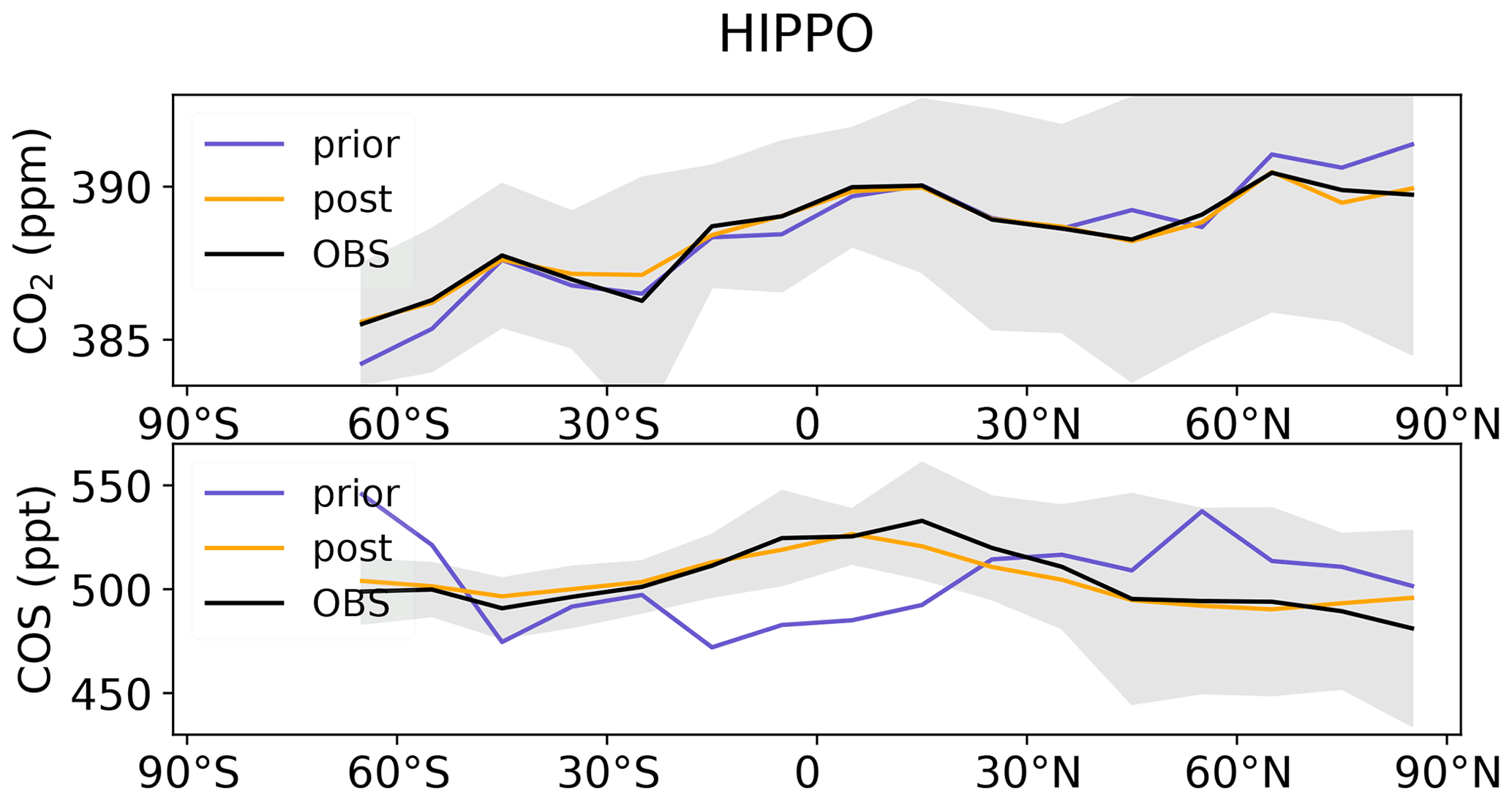
Figure 10Comparison of the latitudinal variations in the a priori and a posteriori LMDz COS abundance with the HIPPO observations. Because of the unbalanced prior, the LMDz COS abundances have been vertically shifted such that the means of the a priori are the same as the mean of the HIPPO data (521 ppt). The error bar is calculated as the standard variation in the COS concentration averaged over longitudes and heights.
The optimized COS fluxes are now assessed at three surface sites in Japan: Miyakojima (MIY; 24∘80 N, 125∘27 E), Yokohama (YOK; 35∘51 N, 139∘48 E) and Otaru (OTA; 43∘14 N, 141∘16 E). These measurements are mainly broadscale and should therefore be fairly reproduced by the LMDz ATM. In winter, the confrontation of the posterior concentrations against the measurements serves to evaluate the spatial distribution of the Zumkehr et al. (2018) anthropogenic inventory over the eastern part of China. The same comparison analysis in summer serves to evaluate the posterior oceanic fluxes as these measurements sample ocean air masses. In winter, these sites sample air masses coming from the northeastern edge of China (see Hattori et al., 2020, and the LMDz footprints in Fig. S11). In Fig. 11a and b, we show a comparison between the a posteriori and observed COS concentrations at each of the three sites for both winter and summer 2019. The averaged COS surface concentrations during February–March 2019 and July–August 2019 are also shown in Fig. 11. At the northernmost site OTA, the overestimation of the COS mixing ratios of 40 ppt points at too strong anthropogenic sources in northern China in the modified Zumkehr et al. (2018) inventory. The site located in central Japan, YOK, has a simulated concentration of almost 100 ppt higher than the observations. This implies an error in the inventory, which indicates a source above the site (see Fig. S9). As for the southern site MIY, the model underestimates the COS concentration by 100 ppt, pointing at an underestimation of the anthropogenic sources over the eastern edge of China or the Korean Peninsula.
In summer, sites YOK and OTA sample air masses coming both from continental Japan and from the Pacific Ocean to the east of Japan. The southernmost site MIY seems to be mostly affected by oceanic sources originating from the east (see the LMDz footprints in Fig. S12). The sites OTA and YOK overestimate the COS concentrations by 60 and 150 ppt and reflect the influence of the misplaced anthropogenic source in central Japan (Fig. S13). At MIY, the comparison with observations suggests that the oceanic source is too strong because the atmospheric concentrations are overestimated by 40 ppt in southern Asia and in northern Japan. However, the oceanic source may not be overestimated in southern Asia because we have assumed that CS2 is emitted as COS. Ma et al. (2021) showed that implementing the CS2 oxidation process into the atmosphere leads to a decrease in surface COS mixing ratio of 40 ppt in the vicinity of Japan. Also, there is an oceanic hotspot located in the footprint of the site (see Fig. S13), which might not be reliable.
The spatial pattern of the Zumkehr et al. (2018) inventory seems to show too strong sources over Japan and too weak sources in the eastern edge of China. The inversion system could therefore have compensated for the lack of an anthropogenic source in the eastern part of China by increasing the oceanic source. However, it is difficult to extrapolate conclusions drawn from a specific region to a larger scale. There is also no clear indication that the oceanic sources are overestimated eastward of Japan.
Finally, we perform a similar assessment of the optimized COS fluxes in winter at the station GIF in France. Measurements at the site GIF represent background values of COS in western Europe, and no COS anthropogenic sources have been detected near by Belviso et al. (2020). The footprint of the station covers central France and countries at the eastern edge such as Belgium and the eastern part of Switzerland (see Fig. S14). The confrontation of the posterior concentrations against measurements serves to evaluate the Zumkehr et al. (2018) anthropogenic inventory and, in particular, its spatial distribution over central France since the terrestrial sink is assumed to be much smaller. Station MHD provides very small constraints over France and eastern Europe as its footprint is mainly oceanic. The comparison between the posterior concentrations and atmospheric measurements in Fig. 11c indicates that the anthropogenic sources within the footprint of the station are also overestimated: the a posteriori concentrations are more than 130 ppt higher than the one observed. This confirms the study of Belviso et al. (2020), who reported a misplaced hotspot on Paris (see Fig. S14). In reality, the concentrations at GIF are 10 ppt lower than those at the background MHD, reflecting a dominant influence of the biospheric sink in this season.

Figure 11Mean COS concentration sampled at the first level of the LMDz model in (a) winter 2019 (February, March), (b) in summer 2019 (July–August) and (c) in winter (December–February) during the period 2016–2019. The values within the yellow frames correspond to the mean COS observed and modelled COS concentrations and their standard deviation at four surface sites: Miyakojima (24∘80 N, 125∘27 E), Yokohama (35∘51 N, 139∘48 E), Otaru (43∘14 N, 141∘16 E) and GIF (48∘42′ N–2∘08′ E). The station MHD has been assimilated and is shown here as a reference.
To conclude, there is a need for continuous in situ carbonyl sulfide observations. The lack of continuous in situ observations, especially over the tropics, limits our capacity to infer the COS surface fluxes by inverse modelling and therefore to optimize GPP. There is some hope that new satellite products could address this issue, but at this stage, current COS retrievals also have their limitations such as, for instance, cloud interference or the lack of sensitivity to the surface fluxes (Serio et al., 2021; Glatthor et al., 2017; Kuai et al., 2015b; Vincent and Dudhia, 2017). Setting aside this obvious lack of observations to be assimilated, we are now discussing the way forward to improve our knowledge of the COS budget.
-
Improving the anthropogenic inventory. The inverse system has weakened the global anthropogenic source by almost 20 %. It is unclear whether this decrease results from an overestimation of the global emissions or from misplaced hotspots within the footprints of the assimilated stations. For instance, the overestimated concentrations in the model at a site located in central Japan point to a misplaced hotspot near the station. If these measurements were assimilated, the inverse system would tend to produce an unrealistic negative flux increment over the area to match the observed concentrations. A similar inconsistency has been reported between measurements at the Gif-sur-Yvette background site and the hotspot to the north, over Paris, stated in the Zumkehr et al. (2018) inventory. Thus, the reported hotspot locations and magnitudes must be improved to be able to benefit from these new observations at Gif-sur-Yvette and in Japan. Further work should include a more thorough evaluation of European anthropogenic sources using COS retrievals from Fourier transform infrared spectrometry (Wang et al., 2016; Krysztofiak et al., 2015) along with a high-resolution (e.g., 0.5∘) chemical transport model in order to correct the spatial distribution of these emissions. Samples in industrial facilities could also be made to validate anthropogenic inventories. Currently, due to large uncertainties in the emission factors and the use of a proxy for spatial disaggregation, the anthropogenic inventory is more appropriate for interpreting atmospheric COS measurements from background sites like MLO than atmospheric COS measurements which have a significant influence from nearby emissions (e.g., Japan/YOK).
-
Improving the relationship between COS plant uptake and GPP. For the LRU values, we have only made a distinction between C4 and C3 plants. A complementary experiment would be to optimize a set of LRU coefficients for each PFT together with the GPP fluxes. We plan to include the PFT dependence of the LRU by using the LRU dataset of Maignan et al. (2020) derived from a mechanistic vegetation model and for which conductances will be further tuned with eddy covariance flux measurements. LRU absolute values are indeed critical. For instance, if the LRU were larger at high latitude, the inversion would not need to increase the GPP as much. However, LRUs have been estimated to be lower in the boreal ecosystems (around 1 and 1.8 for Maignan et al. (2020) and Seibt et al. (2010), respectively) than in the tropical and temperate ecosystems (around 1.3 and 3 for Maignan et al. (2020) and Seibt et al. (2010), respectively). So, using another existing LRU dataset will likely lead to a comparable GPP sink in the high latitudes. Another simplification of our study is that the current LRU approach does not take into account the feedback between COS vegetation sink and atmospheric concentrations. The atmospheric concentrations vary on seasonal and interannual timescales but have indeed been considered constant per latitudinal band. Such a feedback might have a significant impact on the total vegetation sink (see Fig. S18), in particular over the Amazon. Thus, refining our inverse system would require including the feedback between the atmospheric concentrations and the COS vegetation sink (first-order approach). This will involve representing the sharp drop of COS between the canopy and the boundary layer, which can reach 70 ppt in redwood forests (Campbell et al., 2015). However, current global models do not represent the turbulence within the canopy and the link with the atmospheric boundary layer, which does not allow us to correctly simulate the vertical gradient of concentrations between the lowest layer of an atmospheric model and the canopy. Some promising developments were made with the ORCHIDEE LSM (Naudts et al., 2015), but more research is needed before they can be used for our application.
-
Increasing the realism of the soil fluxes. The GPP estimate strongly relies on the realism of the soil fluxes. The soil fluxes need to be more constrained and their errors better defined. In particular, more attention should be paid to the seasonality of soil fluxes compared to that of the vegetation fluxes in the field measurements. For instance, this would help to know whether the 2-month lag between the soil and vegetation fluxes in the high latitudes is realistic.
-
Improving the prior COS oceanic fluxes with the help of an ocean model. Prior oceanic emissions are probably overestimated in the high latitudes and mid-latitudes as shown by Lennartz et al. (2017, 2020a) and as suggested by the inverse system. A possible reason could be the lack of horizontal transport and downward mixing within the water column in their ocean box model. Another estimation of the oceanic emissions based on an ocean general circulation and biogeochemistry model which fully represents the transport of water masses would help to better define the range of uncertainties of these emissions. In particular, the DMS emissions simulated by the NEMO PISCES ocean model (Belviso et al., 2012) are higher over most oligotrophic subtropical zones compared to the DMS emissions of Lana et al. (2011). This means that the spatial distribution of the DMS oceanic emissions is highly uncertain. In the past, direct oceanic emissions have been simulated in the Nucleus for European Modelling of the Ocean (NEMO) Pelagic Interaction Scheme for Carbon and Ecosystem Studies (PISCES) ocean model by Launois et al. (2015a), but the hydrolysis rate has later been found to be erroneous. Future work should include the correction of the rate in the NEMO-PISCES ocean model and also the implementation of the oceanic physical processes responsible for the CS2 emissions. Moreover, the single factor used to convert DMS into COS is very uncertain and may not apply to any atmospheric conditions (Von Hobe, M., personal communication, 2020). Since there is so much DMS emitted by the ocean (ca. 28 TgS yr−1), a small change in the conversion factor (e.g., from the current 0.7 % to 2.5 %) could make a large difference. When the relative contribution of indirect COS sources to total ocean emissions is better known, an extension of this work could be to optimize each oceanic process separately.
-
Implementing a complete chemistry of COS into the LMDz atmospheric transport model. For an economy of computation time, we have assumed that the DMS and CS2 oxidation into COS happens instantly in the atmosphere. However, Ma et al. (2021) showed that such simplifications could modify the average COS surface concentrations up to 80 ppt over eastern China and Japan in winter. These chemical reactions need to be implemented in the LMDz atmospheric model in order to properly evaluate the Zumkehr et al. (2018) inventory with the help of COS atmospheric measurements. The lifetime of the DMS, CS2 and, to a lesser extent, COS into the atmosphere depends on the realism of the OH fields. Therefore, the impact of their uncertainty on the inverse results also needs to be quantified. Chemical transport models disagree on the spatial distribution of the OH fields, and using other OH fields could significantly alter the COS budget as was demonstrated for the methane budget (Zhao et al., 2020a, b). In addition, we plan to introduce the stratospheric chemistry of COS into the LMDz atmospheric transport model. The implementation of a complete chemistry while keeping a multi-year inversion window requires using a variational approach: the chemical reactions are indeed more difficult to implement in an analytical inverse system using pre-computed Jacobian matrices.
-
Including potentially important missing sources. For instance, the biomass burning sources from biofuels are not included in the Stinecipher et al. (2019) inventory, although they were previously estimated to be three times as large as the sources from open burning (Campbell et al., 2015). We have also neglected the contribution of volcanic emissions on the COS budget. As the locations and time of the volcanic eruptions are well known, emissions based on existing measurements (Belviso et al., 1986; Chiodini et al., 1991; Symonds et al., 1992; Sawyer et al., 2008; Notsu and Mori, 2010) could be mapped and given as an input to the atmospheric model. Likewise, DMS emissions from vegetation, tropical forests, soil and wetlands (Yi et al., 2008; Kanda et al., 1992; Minami et al., 1993) have not been included, although their contribution to the total DMS release have been estimated in the past to be between 2 % and 15 % (Watts, 2000; Gondwe et al., 2003). Moreover, we have neglected the COS emissions from the anoxic soils that might be a part of the missing tropical source, in particular within the waterlogged soils of the rice paddies (Yi et al., 2008).
We have developed an analytical system that optimizes GPP, plant respiration CO2 flux and COS soil fluxes within the 15 PFTs defined in the ORCHIDEE terrestrial model, enabling us to take into account the ecosystem dependence of the fluxes. The LRU approach was used to link the GPP to the COS plant uptake. With this system, we have performed a joint assimilation of CO2 and COS atmospheric measurements into the LMDz atmospheric transport model for the period 2008–2019. From a technical point of view, the inverse system is able to find the components of the CO2 and COS budgets that give a good fit with assimilated measurements. Inverse results point at a large oceanic COS source between 450 and 600 GgS yr−1, most of it located in the tropics. The inversion leads to a GPP increase of a few gigatonnes of carbon in the high latitudes and a decrease on the same order of magnitude in the lower latitudes (tropics and mid-latitudes) compared to the initial prior estimates from the ORCHIDEE LSM. For COS, this means a vegetation sink of around −620 GgS yr−1, which is in the lower range of recent estimates based on top-down approaches (Launois et al., 2015b: −663–772 GgS yr−1; Ma et al., 2021: −557–1053 GgS yr−1). The soil sink and the anthropogenic sources have both decreased and amount to −210 and 335 GgS yr−1, respectively. Biomass burning emissions have been slightly revised upward to 65 GgS yr−1. Compared to GPP, plant respiration has almost not been affected in the high latitudes whereas its total value has decreased by only one-quarter of the change in GPP in lower latitudes. The resulting CO2 biospheric fluxes, defined here as the sum of the respiration and GPP, have lost 2 GtC yr−1 above 30∘ N compared to the prior fluxes simulated by the ORCHIDEE LSM. This behaviour is shared by current inverse systems which infer the net CO2 fluxes from atmospheric CO2 measurements (Friedlingstein et al., 2020).
Several aspects of the inferred COS fluxes, such as the inter-hemispheric gradient, the tropical spatial distribution, and the anthropogenic emissions over Japan, China and France, were evaluated with independent atmospheric measurements over different parts of the globe. In the tropics, independent observations of the upper-troposphere COS partial column and the SIF weaken our confidence in the change in tropical GPP; the inverse system actually lacks measurements in this area to ensure a robust partitioning between the oceanic and the continental components of the COS budget. Indeed, the footprint map of the assimilated measurements indicates that the tropical areas, in particular the continents, are poorly constrained by the inverse system. The inverse system partly relies on the terrestrial reference fluxes and adjusts the tropical source to match the surface measurements over the tropics. If the tropical oceanic release is indeed underestimated in the reference fluxes, its magnitude remains highly uncertain. In contrast, in the high latitudes, independent measurements suggest that the inversion has rightly corrected an underestimation of the GPP in the ORCHIDEE land surface model. Concerning the COS anthropogenic sources, Japanese measurements suggest that these are underestimated in eastern China, highlighting the need for an improved anthropogenic inventory.
| PFT | Abbreviation |
| Bare soil | BaS |
| Tropical broadleaved evergreen forest | TrBrE |
| Tropical broadleaved raingreen forest | TrBrR |
| Temperate needleleaf evergreen forest | TeNeE |
| Temperate broadleaved evergreen forest | TeBrE |
| Temperate broadleaved summergreen forest | TrBrS |
| Boreal needleleaf evergreen forest | BoNeE |
| Boreal broadleaved summergreen forest | BoBrS |
| Boreal needleleaf summergreen forest | BoNeS |
| Temperate C3 grass | TeC3g |
| C4 grass | C4g |
| C3 agriculture | C3Ag |
| C4 agriculture | C4Ag |
| Tropical C3 grass | TrC3g |
| Boreal C3 grass | BoC3g |
The COS MIPAS retrievals are available from http://www.imk-asf.kit.edu/english/308.php (last access: 7 February 2022). The LMDz model is available from http://svn.lmd.jussieu.fr/LMDZ/LMDZ6/ under the CeCILL v2 free software license. The COS time series at station GIF from 2014 to 2019 are provided by Sauveur Belviso and can be downloaded from https://sharebox.lsce.ipsl.fr/index.php/s/Yxbj6dZsrc6nsOZ?path=2FGIF-observations (last access: 22 February 2022).
The supplement related to this article is available online at: https://doi.org/10.5194/acp-22-2525-2022-supplement.
MR, FC and PP conceived the research with contributions from SB. MR built the analytical inverse system and conducted the analysis. AP helped in the analysis of the simulation outputs. CA and FM conducted the ORCHIDEE simulations. SL provided the oceanic fluxes of COS and CS2. SB provided the observations at the GIF site. AB developed the facility used to compute the observation footprints. CB and FM were consulted on their expertise of the SIF data. All coauthors reviewed the paper.
The contact author has declared that neither they nor their co-authors have any competing interests.
Publisher’s note: Copernicus Publications remains neutral with regard to jurisdictional claims in published maps and institutional affiliations.
This study was funded by the CO2 Human Emissions (CHE) project, which received funding from the European Union's Horizon 2020 research and innovation programme under grant agreement no. 776186. The authors kindly thank the scientists who provided the measurements used in this study. In particular, the MIPAS averaging kernels were provided by Michael Kiefer. The surface measurements from the NOAA network have been performed by scientists affiliated with NOAA (Stephen Montzka, Carolina Siso, John B. Miller, Fred Moore). The airborne measurements from HIPPO have been made with the help of Eliott L. Atlas at the University of Miami (for the HIPPO campaign). Dan Yakir facilitates the collection of flask samples at WIS. Shohei Hattori facilitates the collection of flask samples over Japan.
This research has been supported by the H2020 Innovation In SMEs (grant no. 776186).
This paper was edited by Anita Ganesan and reviewed by J. Elliott Campbell and one anonymous referee.
Abadie, C., Maignan, F., Remaud, M., Ogée, J., Campbell, J. E., Whelan, M. E., Kitz, F., Spielmann, F. M., Wohlfahrt, G., Wehr, R., Sun, W., Raoult, N., Seibt, U., Hauglustaine, D., Lennartz, S. T., Belviso, S., Montagne, D., and Peylin, P.: Global modelling of soil carbonyl sulfide exchange, Biogeosciences Discuss. [preprint], https://doi.org/10.5194/bg-2021-281, in review, 2021. a
Alemohammad, S. H., Fang, B., Konings, A. G., Aires, F., Green, J. K., Kolassa, J., Miralles, D., Prigent, C., and Gentine, P.: Water, Energy, and Carbon with Artificial Neural Networks (WECANN): a statistically based estimate of global surface turbulent fluxes and gross primary productivity using solar-induced fluorescence, Biogeosciences, 14, 4101–4124, https://doi.org/10.5194/bg-14-4101-2017, 2017. a
Anav, A., Friedlingstein, P., Beer, C., Ciais, P., Harper, A., Jones, C., Murray‐Tortarolo, G., Papale, D., Parazoo, N. C., Peylin, P., Piao, S., Sitch, S., Viovy, N., Wiltshire, A., and Zhao, M.: Spatiotemporal patterns of terrestrial gross primary production: A review, Rev. Geophys., 53, 785–818, https://doi.org/10.1002/2015RG000483, 2015. a, b
Aydin, M., Britten, G. L., Montzka, S. A., Buizert, C., Primeau, F., Petrenko, V., Battle, M. B., Nicewonger, M. R., Patterson, J., Hmiel, B., and Saltzman, E. S.: Anthropogenic Impacts on Atmospheric Carbonyl Sulfide Since the 19th Century Inferred From Polar Firn Air and Ice Core Measurements, J. Geophys. Res.-Atmos., 125, e2020JD033074, https://doi.org/10.1029/2020JD033074, 2020. a
Bacour, C., Maignan, F., Peylin, P., MacBean, N., Bastrikov, V., Joiner, J., Köhler, P., Guanter, L., and Frankenberg, C.: Differences Between OCO-2 and GOME-2 SIF Products From a Model-Data Fusion Perspective, J. Geophys. Res.-Biogeo., 124, 3143–3157, https://doi.org/10.1029/2018JG004938, 2019. a
Badgley, G., Anderegg, L. D. L., Berry, J. A., and Field, C. B.: Terrestrial gross primary production: Using NIRV to scale from site to globe, Global Change Biol., 25, 3731–3740, https://doi.org/10.1111/gcb.14729, 2019. a
Barnes, I., Becker, K. H., and Patroescu, I.: FTIR product study of the OH initiated oxidation of dimethyl sulphide: Observation of carbonyl sulphide and dimethyl sulphoxide, Atmos. Environ., 30, 1805–1814, https://doi.org/10.1016/1352-2310(95)00389-4, 1996. a
Beer, C., Ciais, P., Reichstein, M., Baldocchi, D., Law, B. E., Papale, D., Soussana, J.-F., Ammann, C., Buchmann, N., Frank, D., Gianelle, D., Janssens, I. A., Knohl, A., Köstner, B., Moors, E., Roupsard, O., Verbeeck, H., Vesala, T., Williams, C. A., and Wohlfahrt, G.: Temporal and among-site variability of inherent water use efficiency at the ecosystem level, Global Biogeochem. Cy., 23, https://doi.org/10.1029/2008GB003233, 2009. a
Beer, C., Reichstein, M., Tomelleri, E., Ciais, P., Jung, M., Carvalhais, N., Rödenbeck, C., Arain, M. A., Baldocchi, D., Bonan, G. B., Bondeau, A., Cescatti, A., Lasslop, G., Lindroth, A., Lomas, M., Luyssaert, S., Margolis, H., Oleson, K. W., Roupsard, O., Veenendaal, E., Viovy, N., Williams, C., Woodward, F. I., and Papale, D.: Terrestrial gross carbon dioxide uptake: global distribution and covariation with climate, Science, 329, 834–838, https://doi.org/10.1126/science.1184984, 2010. a
Belviso, S., Nguyen, B. C., and Allard, P.: Estimate of carbonyl sulfide (OCS) volcanic source strength deduced from OCS/CO2 ratios in volcanic gases, Geophys. Res. Lett., 13, 133–136, https://doi.org/10.1029/GL013i002p00133, 1986. a
Belviso, S., Masotti, I., Tagliabue, A., Bopp, L., Brockmann, P., Fichot, C., Caniaux, G., Prieur, L., Ras, J., Uitz, J., Loisel, H., Dessailly, D., Alvain, S., Kasamatsu, N., and Fukuchi, M.: DMS dynamics in the most oligotrophic subtropical zones of the global ocean, Biogeochemistry, 110, 215–241, https://doi.org/10.1007/s10533-011-9648-1, 2012. a
Belviso, S., Lebegue, B., Ramonet, M., Kazan, V., Pison, I., Berchet, A., Delmotte, M., Yver-Kwok, C., Montagne, D., and Ciais, P.: A top-down approach of sources and non-photosynthetic sinks of carbonyl sulfide from atmospheric measurements over multiple years in the Paris region (France), PLOS ONE, 15, e0228419, https://doi.org/10.1371/journal.pone.0228419, 2020. a, b, c, d, e
Berchet, A., Sollum, E., Thompson, R. L., Pison, I., Thanwerdas, J., Broquet, G., Chevallier, F., Aalto, T., Berchet, A., Bergamaschi, P., Brunner, D., Engelen, R., Fortems-Cheiney, A., Gerbig, C., Groot Zwaaftink, C. D., Haussaire, J.-M., Henne, S., Houweling, S., Karstens, U., Kutsch, W. L., Luijkx, I. T., Monteil, G., Palmer, P. I., van Peet, J. C. A., Peters, W., Peylin, P., Potier, E., Rödenbeck, C., Saunois, M., Scholze, M., Tsuruta, A., and Zhao, Y.: The Community Inversion Framework v1.0: a unified system for atmospheric inversion studies, Geosci. Model Dev., 14, 5331–5354, https://doi.org/10.5194/gmd-14-5331-2021, 2021. a
Berndt, T., Scholz, W., Mentler, B., Fischer, L., Hoffmann, E. H., Tilgner, A., Hyttinen, N., Prisle, N. L., Hansel, A., and Herrmann, H.: Fast Peroxy Radical Isomerization and OH Recycling in the Reaction of OH Radicals with Dimethyl Sulfide, J. Phys. Chem. Lett., 10, 6478–6483, https://doi.org/10.1021/acs.jpclett.9b02567, 2019. a
Berry, J., Wolf, A., Campbell, J. E., Baker, I., Blake, N., Blake, D., Denning, A. S., Kawa, S. R., Montzka, S. A., Seibt, U., Stimler, K., Yakir, D., and Zhu, Z.: A coupled model of the global cycles of carbonyl sulfide and CO2: A possible new window on the carbon cycle, J. Geophys. Res.-Biogeo., 118, 842–852, https://doi.org/10.1002/jgrg.20068, 2013a. a, b, c, d, e, f, g, h, i, j
Berry, J., Wolf, A., Campbell, J. E., Baker, I., Blake, N., Blake, D., Denning, A. S., Kawa, S. R., Montzka, S. A., Seibt, U., Stimler, K., Yakir, D., and Zhu, Z.: A coupled model of the global cycles of carbonyl sulfide and CO2: A possible new window on the carbon cycle, Geophys. Res.-Biogeo., 118, 842–852, https://doi.org/10.1002/jgrg.20068, 2013b. a
Blake, N. J., Streets, D. G., Woo, J.-H., Simpson, I. J., Green, J., Meinardi, S., Kita, K., Atlas, E., Fuelberg, H. E., Sachse, G., Avery, M. A., Vay, S. A., Talbot, R. W., Dibb, J. E., Bandy, A. R., Thornton, D. C., Rowland, F. S., and Blake, D. R.: Carbonyl sulfide and carbon disulfide: Large-scale distributions over the western Pacific and emissions from Asia during TRACE-P, J. Geophys. Res.-Atmos., 109, D15S05, https://doi.org/10.1029/2003JD004259, 2004. a
Blake, N. J., Campbell, J. E., Vay, S. A., Fuelberg, H. E., Huey, L. G., Sachse, G., Meinardi, S., Beyersdorf, A., Baker, A., Barletta, B., Midyett, J., Doezema, L., Kamboures, M., McAdams, J., Novak, B., Rowland, F. S., and Blake, D. R.: Carbonyl sulfide (OCS): Large-scale distributions over North America during INTEX-NA and relationship to CO2, J. Geophys. Res.-Atmos., 113, D09S90, https://doi.org/10.1029/2007JD009163, 2008. a
Campbell, J. E., Carmichael, G. R., Chai, T., Mena-Carrasco, M., Tang, Y., Blake, D. R., Blake, N. J., Vay, S. A., Collatz, G. J., Baker, I., Berry, J. A., Montzka, S. A., Sweeney, C., Schnoor, J. L., and Stanier, C. O.: Photosynthetic Control of Atmospheric Carbonyl Sulfide During the Growing Season, Science, 322, 1085–1088, https://doi.org/10.1126/science.1164015, 2008. a, b
Campbell, J. E., Whelan, M. E., Seibt, U., Smith, S. J., Berry, J. A., and Hilton, T. W.: Atmospheric carbonyl sulfide sources from anthropogenic activity: Implications for carbon cycle constraints, Geophys. Res. Lett., 42, 3004–3010, https://doi.org/10.1002/2015GL063445, 2015. a, b, c
Campbell, J. E., Berry, J. A., Seibt, U., Smith, S. J., Montzka, S. A., Launois, T., Belviso, S., Bopp, L., and Laine, M.: Large historical growth in global terrestrial gross primary production, Nature, 544, 84–87, https://doi.org/10.1038/nature22030, 2017. a
Chevallier, F.: Impact of correlated observation errors on inverted CO2 surface fluxes from OCO measurements, Geophys. Res. Lett., 34, L24804, https://doi.org/10.1029/2007GL030463, 2007. a
Chevallier, F.: On the statistical optimality of CO2 atmospheric inversions assimilating CO2 column retrievals, Atmos. Chem. Phys., 15, 11133–11145, https://doi.org/10.5194/acp-15-11133-2015, 2015. a
Chevallier, F., Engelen, R. J., and Peylin, P.: The contribution of AIRS data to the estimation of CO2 sources and sinks, Geophys. Res. Lett., 32, L23801, https://doi.org/10.1029/2005GL024229, 2005. a
Chevallier, F., Ciais, P., Conway, T. J., Aalto, T., Anderson, B. E., Bousquet, P., Brunke, E. G., Ciattaglia, L., Esaki, Y., Fröhlich, M., Gomez, A., Gomez‐Pelaez, A. J., Haszpra, L., Krummel, P. B., Langenfelds, R. L., Leuenberger, M., Machida, T., Maignan, F., Matsueda, H., Morguí, J. A., Mukai, H., Nakazawa, T., Peylin, P., Ramonet, M., Rivier, L., Sawa, Y., Schmidt, M., Steele, L. P., Vay, S. A., Vermeulen, A. T., Wofsy, S., and Worthy, D.: CO2 surface fluxes at grid point scale estimated from a global 21 year reanalysis of atmospheric measurements, J. Geophys. Res.-Atmos., 115, D21307, https://doi.org/10.1029/2010JD013887, 2010. a
Chiodini, G., Cioni, R., Raco, B., and Scandiffio, G.: Carbonyl sulphide (cos) in geothermal fluids: an example from the Larderello field (Italy), Geothermics, 20, 319–327, https://doi.org/10.1016/0375-6505(91)90023-O, 1991. a
Commane, R., Meredith, L. K., Baker, I. T., Berry, J. A., Munger, J. W., Montzka, S. A., Templer, P. H., Juice, S. M., Zahniser, M. S., and Wofsy, S. C.: Seasonal fluxes of carbonyl sulfide in a midlatitude forest, P. Natl. Acad. Sci. USA, 112, 14162–14167, https://doi.org/10.1073/pnas.1504131112, 2015. a, b
Denvil-Sommer, A., Gehlen, M., Vrac, M., and Mejia, C.: LSCE-FFNN-v1: a two-step neural network model for the reconstruction of surface ocean pCO2 over the global ocean, Geosci. Model Dev., 12, 2091–2105, https://doi.org/10.5194/gmd-12-2091-2019, 2019. a
Du, Q., Zhang, C., Mu, Y., Cheng, Y., Zhang, Y., Liu, C., Song, M., Tian, D., Liu, P., Liu, J., Xue, C., and Ye, C.: An important missing source of atmospheric carbonyl sulfide: Domestic coal combustion, Geophys. Res. Lett., 43, 8720–8727, https://doi.org/10.1002/2016GL070075, 2016. a
Fischer, H., Birk, M., Blom, C., Carli, B., Carlotti, M., von Clarmann, T., Delbouille, L., Dudhia, A., Ehhalt, D., Endemann, M., Flaud, J. M., Gessner, R., Kleinert, A., Koopman, R., Langen, J., López-Puertas, M., Mosner, P., Nett, H., Oelhaf, H., Perron, G., Remedios, J., Ridolfi, M., Stiller, G., and Zander, R.: MIPAS: an instrument for atmospheric and climate research, Atmos. Chem. Phys., 8, 2151–2188, https://doi.org/10.5194/acp-8-2151-2008, 2008. a, b
Frankenberg, C., Fisher, J. B., Worden, J., Badgley, G., Saatchi, S. S., Lee, J.-E., Toon, G. C., Butz, A., Jung, M., Kuze, A., and Yokota, T.: New global observations of the terrestrial carbon cycle from GOSAT: Patterns of plant fluorescence with gross primary productivity, Geophys. Res. Lett., 38, L17706, https://doi.org/10.1029/2011GL048738, 2011. a
Friedlingstein, P., O'Sullivan, M., Jones, M. W., Andrew, R. M., Hauck, J., Olsen, A., Peters, G. P., Peters, W., Pongratz, J., Sitch, S., Le Quéré, C., Canadell, J. G., Ciais, P., Jackson, R. B., Alin, S., Aragão, L. E. O. C., Arneth, A., Arora, V., Bates, N. R., Becker, M., Benoit-Cattin, A., Bittig, H. C., Bopp, L., Bultan, S., Chandra, N., Chevallier, F., Chini, L. P., Evans, W., Florentie, L., Forster, P. M., Gasser, T., Gehlen, M., Gilfillan, D., Gkritzalis, T., Gregor, L., Gruber, N., Harris, I., Hartung, K., Haverd, V., Houghton, R. A., Ilyina, T., Jain, A. K., Joetzjer, E., Kadono, K., Kato, E., Kitidis, V., Korsbakken, J. I., Landschützer, P., Lefèvre, N., Lenton, A., Lienert, S., Liu, Z., Lombardozzi, D., Marland, G., Metzl, N., Munro, D. R., Nabel, J. E. M. S., Nakaoka, S.-I., Niwa, Y., O'Brien, K., Ono, T., Palmer, P. I., Pierrot, D., Poulter, B., Resplandy, L., Robertson, E., Rödenbeck, C., Schwinger, J., Séférian, R., Skjelvan, I., Smith, A. J. P., Sutton, A. J., Tanhua, T., Tans, P. P., Tian, H., Tilbrook, B., van der Werf, G., Vuichard, N., Walker, A. P., Wanninkhof, R., Watson, A. J., Willis, D., Wiltshire, A. J., Yuan, W., Yue, X., and Zaehle, S.: Global Carbon Budget 2020, Earth Syst. Sci. Data, 12, 3269–3340, https://doi.org/10.5194/essd-12-3269-2020, 2020. a, b, c
Geels, C., Gloor, M., Ciais, P., Bousquet, P., Peylin, P., Vermeulen, A. T., Dargaville, R., Aalto, T., Brandt, J., Christensen, J. H., Frohn, L. M., Haszpra, L., Karstens, U., Rödenbeck, C., Ramonet, M., Carboni, G., and Santaguida, R.: Comparing atmospheric transport models for future regional inversions over Europe – Part 1: mapping the atmospheric CO2 signals, Atmos. Chem. Phys., 7, 3461–3479, https://doi.org/10.5194/acp-7-3461-2007, 2007. a, b
Glatthor, N., Höpfner, M., Baker, I. T., Berry, J., Campbell, J. E., Kawa, S. R., Krysztofiak, G., Leyser, A., Sinnhuber, B.-M., Stiller, G. P., Stinecipher, J., and Clarmann, T. V.: Tropical sources and sinks of carbonyl sulfide observed from space, Geophys. Res. Lett., 42, 10082–10090, https://doi.org/10.1002/2015GL066293, 2015. a, b, c, d, e, f, g
Glatthor, N., Höpfner, M., Leyser, A., Stiller, G. P., von Clarmann, T., Grabowski, U., Kellmann, S., Linden, A., Sinnhuber, B.-M., Krysztofiak, G., and Walker, K. A.: Global carbonyl sulfide (OCS) measured by MIPAS/Envisat during 2002–2012, Atmos. Chem. Phys., 17, 2631–2652, https://doi.org/10.5194/acp-17-2631-2017, 2017. a, b, c, d
Gondwe, M., Krol, M., Gieskes, W., Klaassen, W., and Baar, H. D.: The contribution of ocean-leaving DMS to the global atmospheric burdens of DMS, MSA, SO2, and NSS SO4, Global Biogeochem. Cy., 17, 1056, https://doi.org/10.1029/2002GB001937, 2003. a
Guanter, L., Frankenberg, C., Dudhia, A., Lewis, P. E., Gómez-Dans, J., Kuze, A., Suto, H., and Grainger, R. G.: Retrieval and global assessment of terrestrial chlorophyll fluorescence from GOSAT space measurements, Remote Sens. Environ., 121, 236–251, https://doi.org/10.1016/j.rse.2012.02.006, 2012. a
Hattori, S., Kamezaki, K., and Yoshida, N.: Constraining the atmospheric OCS budget from sulfur isotopes, P. Natl. Acad. Sci. USA, 117, 20447–20452, https://doi.org/10.1073/pnas.2007260117, 2020. a, b, c
Hauglustaine, D. A., Hourdin, F., Jourdain, L., Filiberti, M.-A., Walters, S., Lamarque, J.-F., and Holland, E. A.: Interactive chemistry in the Laboratoire de Météorologie Dynamique general circulation model: Description and background tropospheric chemistry evaluation, J. Geophys. Res.-Atmos., 109, D04314, https://doi.org/10.1029/2003JD003957, 2004. a
Hilton, T. W., Whelan, M. E., Zumkehr, A., Kulkarni, S., Berry, J. A., Baker, I. T., Montzka, S. A., Sweeney, C., Miller, B. R., and Elliott Campbell, J.: Peak growing season gross uptake of carbon in North America is largest in the Midwest USA, Nat. Clim. Change, 7, 450–454, https://doi.org/10.1038/nclimate3272, 2017. a
Hourdin, F. and Armengaud, A.: The Use of Finite-Volume Methods for Atmospheric Advection of Trace Species. Part I: Test of Various Formulations in a General Circulation Model, Mon. Weather Rev., 127, 822–837, https://doi.org/10.1175/1520-0493(1999)127<0822:TUOFVM>2.0.CO;2, 1999. a
Hourdin, F. and Talagrand, O.: Eulerian backtracking of atmospheric tracers, I: Adjoint derivation and parametrization of subgrid-scale transport, Q. J. Roy. Meteor. Soc., 132, 567–583, https://doi.org/10.1256/qj.03.198.A, 2006. a
Hourdin, F., Musat, I., Bony, S., Braconnot, P., Codron, F., Dufresne, J.-L., Fairhead, L., Filiberti, M.-A., Friedlingstein, P., Grandpeix, J.-Y., Krinner, G., LeVan, P., Li, Z.-X., and Lott, F.: The LMDZ4 general circulation model: climate performance and sensitivity to parametrized physics with emphasis on tropical convection, Clim. Dynam., 27, 787–813, https://doi.org/10.1007/s00382-006-0158-0, 2006. a
Hourdin, F., Rio, C., Grandpeix, J.-Y., Madeleine, J.-B., Cheruy, F., Rochetin, N., Jam, A., Musat, I., Idelkadi, A., Fairhead, L., Foujols, M.-A., Mellul, L., Traore, A.-K., Dufresne, J.-L., Boucher, O., Lefebvre, M.-P., Millour, E., Vignon, E., Jouhaud, J., Diallo, F. B., Lott, F., Gastineau, G., Caubel, A., Meurdesoif, Y., and Ghattas, J.: LMDZ6A: the atmospheric component of the IPSL climate model with improved and better tuned physics, J. Adv. Model. Earth Sy., 12, e2019MS001892, https://doi.org/10.1029/2019MS001892, 2020. a
Jasechko, S.: Global Isotope Hydrogeology―Review, Rev. Geophys., 57, 835–965, https://doi.org/10.1029/2018RG000627, 2019. a
Joiner, J., Guanter, L., Lindstrot, R., Voigt, M., Vasilkov, A. P., Middleton, E. M., Huemmrich, K. F., Yoshida, Y., and Frankenberg, C.: Global monitoring of terrestrial chlorophyll fluorescence from moderate-spectral-resolution near-infrared satellite measurements: methodology, simulations, and application to GOME-2, Atmos. Meas. Tech., 6, 2803–2823, https://doi.org/10.5194/amt-6-2803-2013, 2013. a
Joiner, J., Yoshida, Y., Guanter, L., and Middleton, E. M.: New methods for the retrieval of chlorophyll red fluorescence from hyperspectral satellite instruments: simulations and application to GOME-2 and SCIAMACHY, Atmos. Meas. Tech., 9, 3939–3967, https://doi.org/10.5194/amt-9-3939-2016, 2016. a, b
Jones, M. W., Andrew, R. M., Peters, G. P., Janssens-Maenhout, G., De-Gol, A. J., Ciais, P., Patra, P. K., Chevallier, F., and Le Quéré, C.: Gridded fossil CO 2 emissions and related O 2 combustion consistent with national inventories 1959–2018, Sci. Data, 8, https://doi.org/10.1038/s41597-020-00779-6, 2021. a
Jung, M., Schwalm, C., Migliavacca, M., Walther, S., Camps-Valls, G., Koirala, S., Anthoni, P., Besnard, S., Bodesheim, P., Carvalhais, N., Chevallier, F., Gans, F., Goll, D. S., Haverd, V., Köhler, P., Ichii, K., Jain, A. K., Liu, J., Lombardozzi, D., Nabel, J. E. M. S., Nelson, J. A., O'Sullivan, M., Pallandt, M., Papale, D., Peters, W., Pongratz, J., Rödenbeck, C., Sitch, S., Tramontana, G., Walker, A., Weber, U., and Reichstein, M.: Scaling carbon fluxes from eddy covariance sites to globe: synthesis and evaluation of the FLUXCOM approach, Biogeosciences, 17, 1343–1365, https://doi.org/10.5194/bg-17-1343-2020, 2020. a, b
Kanda, K.-I., Tsuruta, H., and Minami, K.: Emission of dimethyl sulfide, carbonyl sulfide, and carbon bisulfide from paddy fields, Soil Sci. Plant, 38, 709–716, https://doi.org/10.1080/00380768.1992.10416701, 1992. a
Kettle, A. J., Kuhn, U., Hobe, M. V., Kesselmeier, J., and Andreae, M. O.: Global budget of atmospheric carbonyl sulfide: Temporal and spatial variations of the dominant sources and sinks, J. Geophys. Res.-Atmos., 107, 1–16, https://doi.org/10.1029/2002JD002187, 2002. a, b, c, d, e, f, g, h, i, j
Khalil, M. A. K. and Rasmussen, R. A.: Global sources, lifetimes and mass balances of carbonyl sulfide (OCS) and carbon disulfide (CS2) in the earth's atmosphere, Atmos. Environ., 18, 1805–1813, https://doi.org/10.1016/0004-6981(84)90356-1, 1984. a
Khan, A., Razis, B., Gillespie, S., Percival, C., and Shallcross, D.: Global analysis of carbon disulfide (CS2) using the 3-D chemistry transport model STOCHEM, AIMS Environ. Sci., 4, 484, https://doi.org/10.3934/environsci.2017.3.484 2017. a
Kooijmans, L. M. J., Sun, W., Aalto, J., Erkkilä, K.-M., Maseyk, K., Seibt, U., Vesala, T., Mammarella, I., and Chen, H.: Influences of light and humidity on carbonyl sulfide-based estimates of photosynthesis, P. Natl. Acad. Sci. USA, 116, 2470–2475, https://doi.org/10.1073/pnas.1807600116, 2019. a
Krinner, G., Viovy, N., Noblet-Ducoudré, N. D., Ogée, J., Polcher, J., Friedlingstein, P., Ciais, P., Sitch, S., and Prentice, I. C.: A dynamic global vegetation model for studies of the coupled atmosphere-biosphere system, Global Biogeochem. Cy., 19, GB1015, https://doi.org/10.1029/2003GB002199, 2005. a, b
Krysztofiak, G., Té, Y. V., Catoire, V., Berthet, G., Toon, G. C., Jégou, F., Jeseck, P., and Robert, C.: Carbonyl Sulphide (OCS) Variability with Latitude in the Atmosphere, Atmos. Ocean, 53, 89–101, https://doi.org/10.1080/07055900.2013.876609, 2015. a
Kuai, L., Worden, J. R., Campbell, J. E., Kulawik, S. S., Li, K.-F., Lee, M., Weidner, R. J., Montzka, S. A., Moore, F. L., Berry, J. A., Baker, I., Denning, A. S., Bian, H., Bowman, K. W., Liu, J., and Yung, Y. L.: Estimate of carbonyl sulfide tropical oceanic surface fluxes using Aura Tropospheric Emission Spectrometer observations, J. Geophys. Res.-Atmos., 120, 11012–11023, https://doi.org/10.1002/2015JD023493, 2015a. a, b, c, d, e
Kuai, L., Worden, J. R., Campbell, J. E., Kulawik, S. S., Li, K.-F., Lee, M., Weidner, R. J., Montzka, S. A., Moore, F. L., Berry, J. A., Baker, I., Denning, A. S., Bian, H., Bowman, K. W., Liu, J., and Yung, Y. L.: Estimate of carbonyl sulfide tropical oceanic surface fluxes using Aura Tropospheric Emission Spectrometer observations, J. Geophys. Res.-Atmos., 120, 1012–1023, https://doi.org/10.1002/2015JD023493, 2015b. a
Kuhn, U. and Kesselmeier, J.: Environmental variables controlling the uptake of carbonyl sulfide by lichens, J. Geophys. Res.-Atmos., 105, 26783–26792, https://doi.org/10.1029/2000JD900436, 2000. a
Kuppel, S., Peylin, P., Chevallier, F., Bacour, C., Maignan, F., and Richardson, A. D.: Constraining a global ecosystem model with multi-site eddy-covariance data, Biogeosciences, 9, 3757–3776, https://doi.org/10.5194/bg-9-3757-2012, 2012. a
Lana, A., Bell, T. G., Simó, R., Vallina, S. M., Ballabrera‐Poy, J., Kettle, A. J., Dachs, J., Bopp, L., Saltzman, E. S., Stefels, J., Johnson, J. E., and Liss, P. S.: An updated climatology of surface dimethlysulfide concentrations and emission fluxes in the global ocean, Global Biogeochem. Cy., 25, GB1004, https://doi.org/10.1029/2010GB003850, 2011. a, b
Launois, T., Belviso, S., Bopp, L., Fichot, C. G., and Peylin, P.: A new model for the global biogeochemical cycle of carbonyl sulfide – Part 1: Assessment of direct marine emissions with an oceanic general circulation and biogeochemistry model, Atmos. Chem. Phys., 15, 2295–2312, https://doi.org/10.5194/acp-15-2295-2015, 2015a. a
Launois, T., Peylin, P., Belviso, S., and Poulter, B.: A new model of the global biogeochemical cycle of carbonyl sulfide – Part 2: Use of carbonyl sulfide to constrain gross primary productivity in current vegetation models, Atmos. Chem. Phys., 15, 9285–9312, https://doi.org/10.5194/acp-15-9285-2015, 2015b. a, b, c, d, e, f, g, h, i, j
Lennartz, S. T., Marandino, C. A., von Hobe, M., Cortes, P., Quack, B., Simo, R., Booge, D., Pozzer, A., Steinhoff, T., Arevalo-Martinez, D. L., Kloss, C., Bracher, A., Röttgers, R., Atlas, E., and Krüger, K.: Direct oceanic emissions unlikely to account for the missing source of atmospheric carbonyl sulfide, Atmos. Chem. Phys., 17, 385–402, https://doi.org/10.5194/acp-17-385-2017, 2017. a, b, c, d, e, f, g, h, i
Lennartz, S. T., von Hobe, M., Booge, D., Bittig, H. C., Fischer, T., Gonçalves-Araujo, R., Ksionzek, K. B., Koch, B. P., Bracher, A., Röttgers, R., Quack, B., and Marandino, C. A.: The influence of dissolved organic matter on the marine production of carbonyl sulfide (OCS) and carbon disulfide (CS2) in the Peruvian upwelling, Ocean Sci., 15, 1071–1090, https://doi.org/10.5194/os-15-1071-2019, 2019. a
Lennartz, S. T., Gauss, M., von Hobe, M., and Marandino, C. A.: Monthly resolved modelled oceanic emissions of carbonyl sulphide and carbon disulphide for the period 2000–2019, Earth Syst. Sci. Data, 13, 2095–2110, https://doi.org/10.5194/essd-13-2095-2021, 2021a. a, b, c, d, e, f, g
Lennartz, S. T., Marandino, C. A., von Hobe, M., Andreae, M. O., Aranami, K., Atlas, E., Berkelhammer, M., Bingemer, H., Booge, D., Cutter, G., Cortes, P., Kremser, S., Law, C. S., Marriner, A., Simó, R., Quack, B., Uher, G., Xie, H., and Xu, X.: Marine carbonyl sulfide (OCS) and carbon disulfide (CS2): a compilation of measurements in seawater and the marine boundary layer, Earth Syst. Sci. Data, 12, 591–609, https://doi.org/10.5194/essd-12-591-2020, 2020b. a
Li, X., Xiao, J., and He, B.: Chlorophyll fluorescence observed by OCO-2 is strongly related to gross primary productivity estimated from flux towers in temperate forests, Remote Sens. Environ., 204, 659–671, https://doi.org/10.1016/j.rse.2017.09.034, 2018. a
Locatelli, R., Bousquet, P., Hourdin, F., Saunois, M., Cozic, A., Couvreux, F., Grandpeix, J.-Y., Lefebvre, M.-P., Rio, C., Bergamaschi, P., Chambers, S. D., Karstens, U., Kazan, V., van der Laan, S., Meijer, H. A. J., Moncrieff, J., Ramonet, M., Scheeren, H. A., Schlosser, C., Schmidt, M., Vermeulen, A., and Williams, A. G.: Atmospheric transport and chemistry of trace gases in LMDz5B: evaluation and implications for inverse modelling, Geosci. Model Dev., 8, 129–150, https://doi.org/10.5194/gmd-8-129-2015, 2015. a
Ma, J., Kooijmans, L. M. J., Cho, A., Montzka, S. A., Glatthor, N., Worden, J. R., Kuai, L., Atlas, E. L., and Krol, M. C.: Inverse modelling of carbonyl sulfide: implementation, evaluation and implications for the global budget, Atmos. Chem. Phys., 21, 3507–3529, https://doi.org/10.5194/acp-21-3507-2021, 2021. a, b, c, d, e, f, g, h, i
Maignan, F., Abadie, C., Remaud, M., Kooijmans, L. M. J., Kohonen, K.-M., Commane, R., Wehr, R., Campbell, J. E., Belviso, S., Montzka, S. A., Raoult, N., Seibt, U., Shiga, Y. P., Vuichard, N., Whelan, M. E., and Peylin, P.: Carbonyl sulfide: comparing a mechanistic representation of the vegetation uptake in a land surface model and the leaf relative uptake approach, Biogeosciences, 18, 2917–2955, https://doi.org/10.5194/bg-18-2917-2021, 2021. a, b, c, d
Maseyk, K., Berry, J. A., Billesbach, D., Campbell, J. E., Torn, M. S., Zahniser, M., and Seibt, U.: Sources and sinks of carbonyl sulfide in an agricultural field in the Southern Great Plains, P. Natl. Acad. Sci. USA, 01319132, https://doi.org/10.1073/pnas.1319132111, 2014. a
Meredith, L. K., Boye, K., Youngerman, C., Whelan, M., Ogée, J., Sauze, J., and Wingate, L.: Coupled Biological and Abiotic Mechanisms Driving Carbonyl Sulfide Production in Soils, Soil Syst., 2, 37, https://doi.org/10.3390/soilsystems2030037, 2018. a
Minami, K., Kanda, K.-I., and Tsuruta, H.: Emission of Biogenic Sulfur Gases from Rice Paddies in Japan, in: Biogeochemistry of Global Change: Radiatively Active Trace Gases Selected Papers from the Tenth International Symposium on Environmental Biogeochemistry, San Francisco, 19–24 August 1991, edited by: Oremland, R. S., Springer US, Boston, MA, 405–418, https://doi.org/10.1007/978-1-4615-2812-8_22, 1993. a
Montzka, S. A., Calvert, P., Hall, B. D., Elkins, J. W., Conway, T. J., Tans, P. P., and Sweeney, C.: On the global distribution, seasonality, and budget of atmospheric carbonyl sulfide (COS) and some similarities to CO2, J. Geophys. Res.-Atmos., 112, D09302, https://doi.org/10.1029/2006JD007665, 2007. a, b, c, d, e
Naudts, K., Ryder, J., McGrath, M. J., Otto, J., Chen, Y., Valade, A., Bellasen, V., Berhongaray, G., Bönisch, G., Campioli, M., Ghattas, J., De Groote, T., Haverd, V., Kattge, J., MacBean, N., Maignan, F., Merilä, P., Penuelas, J., Peylin, P., Pinty, B., Pretzsch, H., Schulze, E. D., Solyga, D., Vuichard, N., Yan, Y., and Luyssaert, S.: A vertically discretised canopy description for ORCHIDEE (SVN r2290) and the modifications to the energy, water and carbon fluxes, Geosci. Model Dev., 8, 2035–2065, https://doi.org/10.5194/gmd-8-2035-2015, 2015. a
Notsu, K. and Mori, T.: Chemical monitoring of volcanic gas using remote FT-IR spectroscopy at several active volcanoes in Japan, Appl. Geochem., 25, 505–512, https://doi.org/10.1016/j.apgeochem.2010.01.008, 2010. a
Ogée, J., Sauze, J., Kesselmeier, J., Genty, B., Van Diest, H., Launois, T., and Wingate, L.: A new mechanistic framework to predict OCS fluxes from soils, Biogeosciences, 13, 2221–2240, https://doi.org/10.5194/bg-13-2221-2016, 2016. a
Peylin, P., Bacour, C., MacBean, N., Leonard, S., Rayner, P., Kuppel, S., Koffi, E., Kane, A., Maignan, F., Chevallier, F., Ciais, P., and Prunet, P.: A new stepwise carbon cycle data assimilation system using multiple data streams to constrain the simulated land surface carbon cycle, Geosci. Model Dev., 9, 3321–3346, https://doi.org/10.5194/gmd-9-3321-2016, 2016. a
Poulter, B., MacBean, N., Hartley, A., Khlystova, I., Arino, O., Betts, R., Bontemps, S., Boettcher, M., Brockmann, C., Defourny, P., Hagemann, S., Herold, M., Kirches, G., Lamarche, C., Lederer, D., Ottlé, C., Peters, M., and Peylin, P.: Plant functional type classification for earth system models: results from the European Space Agency's Land Cover Climate Change Initiative, Geosci. Model Dev., 8, 2315–2328, https://doi.org/10.5194/gmd-8-2315-2015, 2015. a
Protoschill-Krebs, G., Wilhelm, C., and Kesselmeier, J.: Consumption of carbonyl sulphide (COS) by higher plant carbonic anhydrase (CA), Atmos. Environ., 30, 3151–3156, https://doi.org/10.1016/1352-2310(96)00026-X, 1996. a
Rastogi, B., Berkelhammer, M., Wharton, S., Whelan, M. E., Itter, M. S., Leen, J. B., Gupta, M. X., Noone, D., and Still, C. J.: Large Uptake of Atmospheric OCS Observed at a Moist Old Growth Forest: Controls and Implications for Carbon Cycle Applications, J. Geophys. Res.-Biogeo., 123, 3424–3438, https://doi.org/10.1029/2018JG004430, 2018. a
Remaud, M., Chevallier, F., Cozic, A., Lin, X., and Bousquet, P.: On the impact of recent developments of the LMDz atmospheric general circulation model on the simulation of CO2 transport, Geosci. Model Dev., 11, 4489–4513, https://doi.org/10.5194/gmd-11-4489-2018, 2018. a, b
Riley, W. J., Randerson, J. T., Foster, P. N., and Lueker, T. J.: Influence of terrestrial ecosystems and topography on coastal CO2 measurements: A case study at Trinidad Head, California, J. Geophys. Res.-Biogeo., 110, G01005, https://doi.org/10.1029/2004JG000007, 2005. a, b
Ryu, Y., Baldocchi, D. D., Kobayashi, H., Ingen, C. V., Li, J., Black, T. A., Beringer, J., Gorsel, E. V., Knohl, A., Law, B. E., and Roupsard, O.: Integration of MODIS land and atmosphere products with a coupled-process model to estimate gross primary productivity and evapotranspiration from 1 km to global scales, Global Biogeochem. Cy., 25, GB4017, https://doi.org/10.1029/2011GB004053, 2011. a
Sandoval-Soto, L., Stanimirov, M., von Hobe, M., Schmitt, V., Valdes, J., Wild, A., and Kesselmeier, J.: Global uptake of carbonyl sulfide (COS) by terrestrial vegetation: Estimates corrected by deposition velocities normalized to the uptake of carbon dioxide (CO2), Biogeosciences, 2, 125–132, https://doi.org/10.5194/bg-2-125-2005, 2005. a
Sawyer, G. M., Carn, S. A., Tsanev, V. I., Oppenheimer, C., and Burton, M.: Investigation into magma degassing at Nyiragongo volcano, Democratic Republic of the Congo, Geochem. Geophys. Geosyst., 9, Q02017, https://doi.org/10.1029/2007GC001829, 2008. a
Seibt, U., Kesselmeier, J., Sandoval-Soto, L., Kuhn, U., and Berry, J. A.: A kinetic analysis of leaf uptake of COS and its relation to transpiration, photosynthesis and carbon isotope fractionation, Biogeosciences, 7, 333–341, https://doi.org/10.5194/bg-7-333-2010, 2010. a, b, c
Serio, C., Masiello, G., Mastro, P., Belviso, S., and Remaud, M.: Seasonal variability of degrees of freedom and its effect over time series and spatial patterns of atmospheric gases from satellite: application to carbonyl sulfide (OCS), Remote Sensing of Clouds and the Atmosphere XXVI, 11859, 11–23, https://doi.org/10.1117/12.2599761, 2021. a
Stimler, K., Montzka, S. A., Berry, J. A., Rudich, Y., and Yakir, D.: Relationships between carbonyl sulfide (COS) and CO2 during leaf gas exchange, New Phytol., 186, 869–878, https://doi.org/10.1111/j.1469-8137.2010.03218.x, 2010. a, b
Stinecipher, J. R., Cameron‐Smith, P. J., Blake, N. J., Kuai, L., Lejeune, B., Mahieu, E., Simpson, I. J., and Campbell, J. E.: Biomass Burning Unlikely to Account for Missing Source of Carbonyl Sulfide, Geophys. Res. Lett., 46, 14912–14920, https://doi.org/10.1029/2019GL085567, 2019. a, b, c, d
Stocker, B. D., Zscheischler, J., Keenan, T. F., Prentice, I. C., Seneviratne, S. I., and Peñuelas, J.: Drought impacts on terrestrial primary production underestimated by satellite monitoring, Nat. Geosci., 12, 264–270, https://doi.org/10.1038/s41561-019-0318-6, 2019. a, b, c
Sun, Y., Frankenberg, C., Jung, M., Joiner, J., Guanter, L., Köhler, P., and Magney, T.: Overview of Solar-Induced chlorophyll Fluorescence (SIF) from the Orbiting Carbon Observatory-2: Retrieval, cross-mission comparison, and global monitoring for GPP, Remote Sens. Environ., 209, 808–823, https://doi.org/10.1016/j.rse.2018.02.016, 2018. a, b
Suntharalingam, P., Kettle, A. J., Montzka, S. M., and Jacob, D. J.: Global 3-D model analysis of the seasonal cycle of atmospheric carbonyl sulfide: Implications for terrestrial vegetation uptake, Geophys. Res. Lett., 35, L19801, https://doi.org/10.1029/2008GL034332, 2008. a, b, c
Sweeney, C., Karion, A., Wolter, S., Newberger, T., Guenther, D., Higgs, J. A., Andrews, A. E., Lang, P. M., Neff, D., Dlugokencky, E., Miller, J. B., Montzka, S. A., Miller, B. R., Masarie, K. A., Biraud, S. C., Novelli, P. C., Crotwell, M., Crotwell, A. M., Thoning, K., and Tans, P. P.: Seasonal climatology of CO2 across North America from aircraft measurements in the NOAA/ESRL Global Greenhouse Gas Reference Network, J. Geophys. Res.-Atmos., 120, 5155–5190, https://doi.org/10.1002/2014JD022591, 2015. a
Symonds, R. B., Reed, M. H., and Rose, W. I.: Origin, speciation, and fluxes of trace-element gases at Augustine volcano, Alaska: Insights into magma degassing and fumarolic processes, Geochim. Cosmochim. Ac., 56, 633–657, https://doi.org/10.1016/0016-7037(92)90087-Y, 1992. a
Tarantola, A.: Inverse problems theory, Methods for Data Fitting and Model Parameter Estimation, Elsevier, Southampton, ISBN 9780444599674, 1989. a
Thoning, K. W., Tans, P. P., and Komhyr, W. D.: Atmospheric carbon dioxide at Mauna Loa Observatory: 2. Analysis of the NOAA GMCC data, 1974–1985, J. Geophys. Res.-Atmos., 94, 8549–8565, https://doi.org/10.1029/JD094iD06p08549, 1989. a
Van Leer, B.: Towards the ultimate conservative difference scheme, IV. A new approach to numerical convection, J. Comput. Phys., 23, 276–299, https://doi.org/10.1016/0021-9991(77)90095-X, 1977. a
Veres, P. R., Neuman, J. A., Bertram, T. H., Assaf, E., Wolfe, G. M., Williamson, C. J., Weinzierl, B., Tilmes, S., Thompson, C. R., Thames, A. B., Schroder, J. C., Saiz-Lopez, A., Rollins, A. W., Roberts, J. M., Price, D., Peischl, J., Nault, B. A., Møller, K. H., Miller, D. O., Meinardi, S., Li, Q., Lamarque, J.-F., Kupc, A., Kjaergaard, H. G., Kinnison, D., Jimenez, J. L., Jernigan, C. M., Hornbrook, R. S., Hills, A., Dollner, M., Day, D. A., Cuevas, C. A., Campuzano-Jost, P., Burkholder, J., Bui, T. P., Brune, W. H., Brown, S. S., Brock, C. A., Bourgeois, I., Blake, D. R., Apel, E. C., and Ryerson, T. B.: Global airborne sampling reveals a previously unobserved dimethyl sulfide oxidation mechanism in the marine atmosphere, P. Natl. Acad. Sci. USA, 117, 4505–4510, https://doi.org/10.1073/pnas.1919344117, 2020. a
Vincent, R. A. and Dudhia, A.: Fast retrievals of tropospheric carbonyl sulfide with IASI, Atmos. Chem. Phys., 17, 2981–3000, https://doi.org/10.5194/acp-17-2981-2017, 2017. a
Wang, Y., Deutscher, N. M., Palm, M., Warneke, T., Notholt, J., Baker, I., Berry, J., Suntharalingam, P., Jones, N., Mahieu, E., Lejeune, B., Hannigan, J., Conway, S., Mendonca, J., Strong, K., Campbell, J. E., Wolf, A., and Kremser, S.: Towards understanding the variability in biospheric CO2 fluxes: using FTIR spectrometry and a chemical transport model to investigate the sources and sinks of carbonyl sulfide and its link to CO2, Atmos. Chem. Phys., 16, 2123–2138, https://doi.org/10.5194/acp-16-2123-2016, 2016. a
Watts, S. F.: The mass budgets of carbonyl sulfide, dimethyl sulfide, carbon disulfide and hydrogen sulfide, Atmos. Environ., 34, 761–779, https://doi.org/10.1016/S1352-2310(99)00342-8, 2000. a
Welp, L. R., Keeling, R. F., Meijer, H. A. J., Bollenbacher, A. F., Piper, S. C., Yoshimura, K., Francey, R. J., Allison, C. E., and Wahlen, M.: Interannual variability in the oxygen isotopes of atmospheric CO2 driven by El Niño, Nature, 477, 579–582, https://doi.org/10.1038/nature10421, 2011. a
Whelan, M. E., Min, D.-H., and Rhew, R. C.: Salt marsh vegetation as a carbonyl sulfide (COS) source to the atmosphere, Atmos. Environ., 73, 131–137, https://doi.org/10.1016/j.atmosenv.2013.02.048, 2013. a
Whelan, M. E., Hilton, T. W., Berry, J. A., Berkelhammer, M., Desai, A. R., and Campbell, J. E.: Carbonyl sulfide exchange in soils for better estimates of ecosystem carbon uptake, Atmos. Chem. Phys., 16, 3711–3726, https://doi.org/10.5194/acp-16-3711-2016, 2016. a
Whelan, M. E., Lennartz, S. T., Gimeno, T. E., Wehr, R., Wohlfahrt, G., Wang, Y., Kooijmans, L. M. J., Hilton, T. W., Belviso, S., Peylin, P., Commane, R., Sun, W., Chen, H., Kuai, L., Mammarella, I., Maseyk, K., Berkelhammer, M., Li, K.-F., Yakir, D., Zumkehr, A., Katayama, Y., Ogée, J., Spielmann, F. M., Kitz, F., Rastogi, B., Kesselmeier, J., Marshall, J., Erkkilä, K.-M., Wingate, L., Meredith, L. K., He, W., Bunk, R., Launois, T., Vesala, T., Schmidt, J. A., Fichot, C. G., Seibt, U., Saleska, S., Saltzman, E. S., Montzka, S. A., Berry, J. A., and Campbell, J. E.: Reviews and syntheses: Carbonyl sulfide as a multi-scale tracer for carbon and water cycles, Biogeosciences, 15, 3625–3657, https://doi.org/10.5194/bg-15-3625-2018, 2018. a, b, c, d, e, f
Wofsy, S. C.: HIAPER Pole-to-Pole Observations (HIPPO): fine-grained, global-scale measurements of climatically important atmospheric gases and aerosols, Philos. T. Roy. Soc. A, 369, 2073–2086, https://doi.org/10.1098/rsta.2010.0313, 2011. a
Yang, X., Tang, J., Mustard, J. F., Lee, J.-E., Rossini, M., Joiner, J., Munger, J. W., Kornfeld, A., and Richardson, A. D.: Solar-induced chlorophyll fluorescence that correlates with canopy photosynthesis on diurnal and seasonal scales in a temperate deciduous forest, Geophys. Res. Lett., 42, 2977–2987, https://doi.org/10.1002/2015GL063201, 2015. a
Yi, Z., Wang, X., Sheng, G., and Fu, J.: Exchange of carbonyl sulfide (OCS) and dimethyl sulfide (DMS) between rice paddy fields and the atmosphere in subtropical China, Agr. Ecosyst. Environ., 123, 116–124, https://doi.org/10.1016/j.agee.2007.05.011, 2008. a, b
Zhang, Y., Guanter, L., Berry, J. A., van der Tol, C., Yang, X., Tang, J., and Zhang, F.: Model-based analysis of the relationship between sun-induced chlorophyll fluorescence and gross primary production for remote sensing applications, Remote Sens. Environ., 187, 145–155, https://doi.org/10.1016/j.rse.2016.10.016, 2016. a
Zhao, Y., Saunois, M., Bousquet, P., Lin, X., Berchet, A., Hegglin, M. I., Canadell, J. G., Jackson, R. B., Deushi, M., Jöckel, P., Kinnison, D., Kirner, O., Strode, S., Tilmes, S., Dlugokencky, E. J., and Zheng, B.: On the role of trend and variability in the hydroxyl radical (OH) in the global methane budget, Atmos. Chem. Phys., 20, 13011–13022, https://doi.org/10.5194/acp-20-13011-2020, 2020a. a
Zhao, Y., Saunois, M., Bousquet, P., Lin, X., Berchet, A., Hegglin, M. I., Canadell, J. G., Jackson, R. B., Dlugokencky, E. J., Langenfelds, R. L., Ramonet, M., Worthy, D., and Zheng, B.: Influences of hydroxyl radicals (OH) on top-down estimates of the global and regional methane budgets, Atmos. Chem. Phys., 20, 9525–9546, https://doi.org/10.5194/acp-20-9525-2020, 2020b. a
Zumkehr, A., Hilton, T. W., Whelan, M., Smith, S., and Campbell, J. E.: Gridded anthropogenic emissions inventory and atmospheric transport of carbonyl sulfide in the U.S., J. Geophys. Res.-Atmos., 122, 2169–2178, https://doi.org/10.1002/2016JD025550, 2017. a
Zumkehr, A., Hilton, T. W., Whelan, M., Smith, S., Kuai, L., Worden, J., and Campbell, J. E.: Global gridded anthropogenic emissions inventory of carbonyl sulfide, Atmos. Environ., 183, 11–19, https://doi.org/10.1016/j.atmosenv.2018.03.063, 2018. a, b, c, d, e, f, g, h, i, j, k, l
- Abstract
- Introduction
- Data and method
- Inverse results
- Discussion and perspectives
- Conclusions
- Appendix A: List of the PFTs as defined in the ORCHIDEE LSM
- Code and data availability
- Author contributions
- Competing interests
- Disclaimer
- Acknowledgements
- Financial support
- Review statement
- References
- Supplement