the Creative Commons Attribution 4.0 License.
the Creative Commons Attribution 4.0 License.
 | 17 Feb 2022
Development and application of a street-level meteorology and pollutant tracking system (S-TRACK)
Huan Zhang
Sunling Gong
Lei Zhang
Jingwei Ni
Jianjun He
Yaqiang Wang
Xu Wang
Lixin Shi
Jingyue Mo
Huabing Ke
Shuhua Lu
A multi-model simulation system for street-level circulation and pollutant tracking (S-TRACK) has been developed by integrating the Weather Research and Forecasting (WRF), the STAR-CCM+ (computational fluid dynamics model – CFD), and the Flexible Particle (FLEXPART) models. The winter wind environmental characteristics and the potential contribution of traffic sources to nearby receptor sites in a city district of China are analysed with the system for January 2019. It is found that complex building layouts change the structure of the wind field and thus have an impact on the transport of pollutants. The wind speed inside the building block is lower than the background wind speed due to the dragging effect of dense buildings. Ventilation is better when the dominant airflow is in the same direction as the building layout. Influenced by the building layout, the local circulations show that the windward side of the building is mostly the divergence zone, and the leeward side is mostly the convergence zone, which is more obvious for high buildings. With the hypothesis that the traffic sources are uniformly distributed on each road and with identical traffic intensity, the potential contribution ratios (PCRs) of four traffic sources to certain specific sites under the influence of the street-level circulations are estimated with the method of residence time analysis. It is found that the contribution ratio varies with the height of the receptor site. As a result of the generally upward motion in the airflow, the position with the greatest PCR from the four road traffic sources is located at a certain height which is commonly influenced by the distance of this location from the traffic source and the background wind field (about 15 m in this study). The potential contribution of a road to one of the receptor sites is also investigated under different wind directions. The established system and the results can be used to understand the characteristics of urban wind environment and to help the air pollution control planning in urban areas.
- Article
(14479 KB) - Full-text XML
- BibTeX
- EndNote


In recent decades, with the continuous development of urban construction in China, urban environmental problems have become increasingly serious and attracted widespread attention. According to the 2019 China Ecological Environment Status Bulletin, 180 of 337 cities at the prefecture level exceeded ambient air quality standards. The complex building layouts and differences in thermal structures within cities lead to extremely complicated meteorological characteristics and pollutant transport in urban areas (Aynsley, 1989; Fernando et al., 2010; Lei et al., 2012). Though the transport of atmospheric pollution in urban areas is widely studied, tracking the sources of pollutants at the street level is still lacking due to limitations in research methods.
Research on the street-level atmospheric environment is mainly divided into three methods: field measurements (Macdonald et al., 1997), laboratory simulation research (Mavroidis et al., 2003), and model simulations (Hendricks et al., 2007; Kochanski et al., 2015; Miao et al., 2014). Model simulation has become one of the main methods for studying environmental problems at the street level due to the easy control of simulation conditions and simple processing steps. Computational fluid dynamics (CFD) is a numerical simulation method to study fluid thermal-dynamic problems and is now widely used in studies related to microscale problems within the urban canopy (Gosman, 1999). The core of the CFD simulation method is to solve the Navier–Stokes equations. Depending on the turbulence closure scheme, CFD models can be divided into three types: direct numerical simulation (DNS), Reynolds-averaged Navier–Stokes (RANS) equations (Liu et al., 2018; Milliez and Carissimo, 2008; Zheng et al., 2015), and large-eddy simulation (LES) (Kurppa et al., 2018; Li et al., 2008; Sada and Sato, 2002). The choice among the three methods depends on the costs and objectives. One of the most important issues using CFD simulation for environment problems at the street level is to obtain accurate initial and boundary conditions (Ehrhard et al., 2000). To solve this problem, the multi-scale coupling method is revealed as a good solution, which uses meteorological information from mesoscale models as the initial and boundary conditions to drive CFD (Nelson et al., 2016). Tewari et al. (2010) proved that CFD simulation was improved significantly when the results of the Weather Research and Forecasting (WRF) model were used as the initial and boundary conditions. With the WRF model, the community multiscale air quality (CMAQ) model, and the CFD (RANS) approach, Kwak et al. (2015) built an urban air quality modelling system, which presented a better performance than the WRF-CMAQ model in simulating nitrogen dioxide (NO2) and ozone (O3) concentrations.
Nevertheless, street-level air pollutant transport resulting from nearby sources was still not fully investigated. The Flexible Particle (FLEXPART) model (Stohl, 2003; Stohl et al., 2005) is a Lagrangian particle dispersion model. The FLEXPART model can track the transport of tracers via forward or backward simulation. Different from an Eulerian model, the Lagrangian model is not restricted by the Courant–Friedrichs–Lewy (CFL) condition (Stam, 1999), and thus, the integration process in the Lagrangian model can be maintained with high spatial resolution with acceptable computation efficiency. Initially, the FLEXPART model was driven by global meteorological reanalysis data from the European Centre for Medium-Range Weather Forecasts (ECMWF) or National Centers for Environmental Prediction (NCEP). Fast and Easter (2006) developed a FLEXPART version that used the WRF model output and was optimized with technical level and output results. Today, the WRF-FLEXPART model has been widely used to research the regional transport of air pollutants (Brioude et al., 2013; De Foy et al., 2011; Gao et al., 2020; J. He et al., 2017; He et al., 2020; Yu et al., 2020). Cécé et al. (2016) first applied the FLEXPART model at a small-scale resolution to analyse potential sources of nitrogen oxide (NOx) in urban areas, with the WRF model results as the driving field. Though FLEXPART has been extensively applied in medium- and long-range transport cases (Heo et al., 2015; Liu et al., 2013; Madala et al., 2015; Sandeepan et al., 2013), it has been rarely tested for street-level transport and small-scale resolution grids.
The objective of the present work is to investigate the flow field characteristics and potential contribution of traffic sources to receptor sites, under real building scenarios and meteorological conditions. To this end, a multi-model simulation system for street-level circulation and pollutant tracking (S-TRACK) was developed by integrating the WRF mesoscale, the STAR-CCM+ street scale, and the FLEXPART particle dispersion models and applying them to the Jinshui District of Zhengzhou City, Henan Province. Zhengzhou is located in central China with four distinct seasons. According to the Oceanic Niño Index (ONI), an El Niño event occurred in January 2019. The occurrence of El Niño generally favours a warm winter and weak winter winds in China that are conducive to the occurrence of air pollution. Therefore, the period of January 2019 was selected and simulated for this study. This paper is organized as follows. Section 2 presents the model details and the observed data for the model validation. Section 3 provides the details of the model validation results, the wind environment characteristics, and the potential contribution of traffic sources to receptor sites in the region. Section 4 provides the conclusions of the study.
2.1 S-TRACK description
The S-TRACK system consists of three major components (Fig. 1). The WRF model is used to obtain the mesoscale three-dimensional (3D) meteorological fields, with the initial and boundary conditions provided by NCEP FNL reanalysis data. STAR-CCM+, driven by the meteorological data from WRF, is used to compute the refined 3D street-level meteorological fields with a resolution of 1 to 100 m in the simulation area. With the refined 3D meteorology, the FLEXPART model is run to analyse the transport of traffic sources at street level and their potential contribution to specific sites. One should note that some meteorological variables needed by FLEXPART that STAR-CCM+ cannot provide (Table 1) are obtained from WRF simulations. The specific coupling scheme of the S-TRACK system is detailed as follows.
- I.
Run the WRF model (refer to Sect. 2.2 for specific settings) to obtain meteorological data with a spatial resolution of 1 km×1 km, including temperature, pressure, humidity, wind, etc.
- II.
Extract the value of temperature (T) and wind (U, V, and W) from the WRF simulation, as the initial and boundary conditions of the STAR-CCM+ simulation. Run STAR-CCM+ (refer to Sect. 2.3 for specific settings) to obtain values of meteorological variables with a spatial resolution of 1–100 m, including wind field, surface pressure, and surface sensible heat flux. The 3D street-level grid for STAR-CCM+ is detailed in Sect. 2.3.1.
- III.
Match the STAR-CCM+ grids to the WRF grids. As the FLEXPART-WRF (version 3.3.2) was used here, the grid structure of meteorological input data to FLEXPART should match the grid structure of the WRF model. To this end, a regular fine grid with a horizontal resolution of 10 m×10 m was constructed based on the pre-processing system of the WRF model (WPS). The urban building height data obtained based on drone aerial photography were taken as part of the terrain height data in the WPS. Once the refined grid was established, the meteorological variables of the STAR-CCM+ and WRF models were interpolated into the grid by a nearest-neighbour interpolation method.
- IV.
Run the backward FLEXPART model (refer to Sect. 2.4 for specific settings) to obtain the 3D spatial location data of released particles, which were used to analyse the features of pollutant transport at street level and the potential contribution of traffic sources to specific sites.
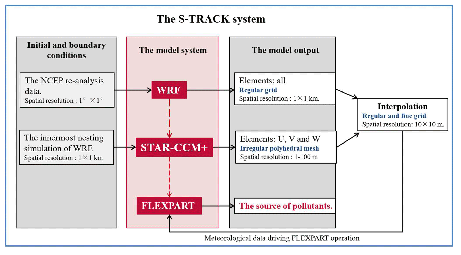
Figure 1The S-TRACK system: the role of WRF, STAR-CCM+, and FLEXPART in the S-TRACK system and the process of gradual refinement of resolution.
Table 1The list of variables required to run FLEXPART and the sources of variables.

2.2 WRF model configuration
In this study, the WRF model is configured with four nested domains (Fig. 2a), with the resolution of 27 km×27 km (85×85 grid cells), 9 km×9 km (82×82 grid cells), 3 km×3 km (82×82 grid cells), and 1 km×1 km (61×61 grid cells). Vertically, there are 45 full eta levels from the surface to 100 hPa, with 11 levels below 2 km, the meteorological fields of which are used to drive STAR-CCM+. The innermost nested region is shown in Fig. 2b, where the area focused in this study is marked with a black box. The initial and boundary conditions of the WRF model are obtained from the NCEP re-analysis data (https://rda.ucar.edu/datasets/ds083.2/, last access: 18 May 2021). The boundary conditions are updated every 6 h. Table 2 lists the selected physical parameterization schemes. The time from 12:00 Beijing time (BJT) on 30 December 2018 to 23:00 BJT on 31 January 2019 is chosen as the modelling period, with the simulation results recorded every hour.
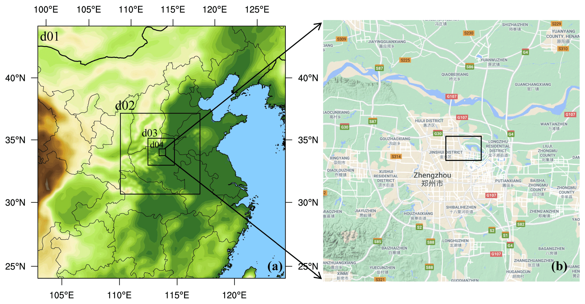
Figure 2Domain configuration of the WRF model: (a) the range of the four nested domains (d1–d4); (b) the innermost nested domain (d4), within which the black box represents the STAR-CCM+ simulation domain (extracted from © Google Maps 2021).
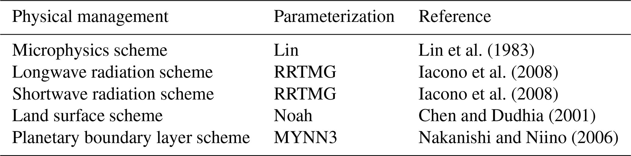
Table 2Parameterization scheme for the physical processes set up in the WRF model.
2.3 STAR-CCM+ configuration
STAR-CCM+, one of the most commonly used commercial CFD softwares, was selected for the street-level simulation. Previous studies had found an excellent correlation between STAR-CCM+ simulated and measured values in simulating environmental and meteorological problems at street level (Borge et al., 2018; Santiago et al., 2020; Santiago et al., 2017). The model has functions such as geometric modelling, model pre-processing, the calculation execution, and post-processing of results. More details on STAR-CCM+ can be found at https://www.plm.automation.siemens.com/global/zh/products/simcenter/STAR-CCM.html (last access: 25 June 2021).
2.3.1 3D street-level grid generation
The establishment of a 3D geometric model is based on the actual terrain and building height data for the simulated area obtained through drone aerial photography technology. Basic data such as the geometric shape of urban buildings, roof height, and vector data of the top of buildings with high resolution, high timeliness, and accuracy are used to construct a realistic 3D geometric model for driving the STAR-CCM+ simulation. In the process of model construction, the same shape as the actual building was maintained to reduce the influence of model errors on the calculation results (Fig. 3a). The length, width, and height of the STAR-CCM+ calculation domain are 13, 11, and 2 km, respectively, among which nearly two-thirds of the buildings are distributed in the range of 10–40 m, with the average height of the buildings being 32 m. The highest building in the area is 390 m, and the lowest building is 6 m.
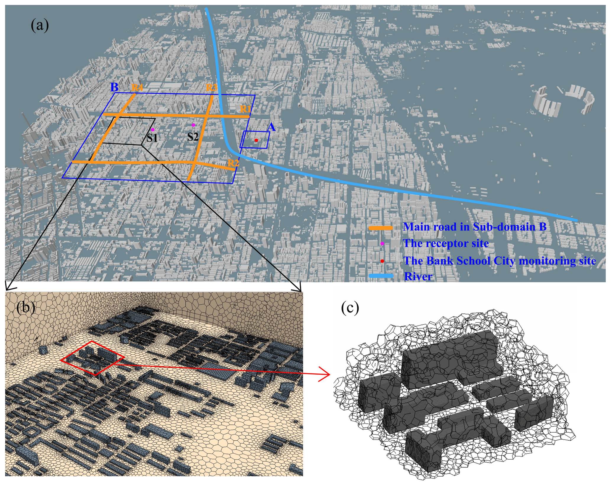
Figure 3The computational domain of STAR-CCM+ is shown in (a). The sub-domain A is used for detailed analysis of the wind environment, and the Bank School City (BSC) monitoring site is marked with the red dot. Sub-domain B is used to analyse the potential contribution of traffic sources to receptor sites in the region, with magenta dots (S1 and S2) indicating the receptor sites and orange lines indicating the main roads. The polyhedral mesh is used to divide the STAR-CCM+ simulation area. The mesh details of the vertical cross section and building surface are shown in (b), and the 3D meshes are shown in (c).
The geometric model domain is divided by polyhedral meshes (Fig. 3c). The polyhedral mesh has much fewer cells than the traditional tetrahedral mesh, but with a similar accuracy of calculation. Under the same number of grid cells, the numerical simulation results of polyhedral grid cells are more consistent with experimental data than tetrahedral grid cells (Zhang et al., 2020). The grid cells on the ground and near the buildings are much denser (Fig. 3b) (the minimum resolution is about 1 m), so that the influence of the building on the flow patterns can be described more accurately. In the end, the number of unit grid cells generated is 382 181, and the number of nodes is 1 990 224.
2.3.2 Physical model and boundary conditions
STAR-CCM+ solves the RANS equations with the realizable k-ε turbulence closure scheme in this study (Lei et al., 2004; L. Li et al., 2006; S. Li et al., 2019). The ground and building surfaces are set to be no-slip, and the distribution of fluid velocity and pressure near the ground and the building surface is described by the blended wall function. For the coupling of the WRF model to STAR-CCM+, the values of temperature and wind from the WRF simulation are extracted to establish the initial and boundary conditions for STAR-CCM+. Since the variables obtained by the WRF simulation have a relatively coarse resolution of 1 km, the velocity components (U, V, and W) and the temperature are interpolated to the boundary of the STAR-CCM+ domain using the spline interpolation method and the linear interpolation method, respectively. For the turbulence intensity and turbulence viscosity ratio, the lateral and upper boundaries are set as constants with values of 0.1 and 10, respectively.
2.4 FLEXPART configuration
The simulation area is set to sub-domain B in Fig. 3, with a horizontal grid resolution of 10 m×10 m. The simulation time is from 01:00 BJT 1 January 2019 to 23:00 BJT 30 January 2019. The time step of FLEXPART is 1 s, and the output time interval is 120 s. Through backward trajectory simulation, the impact of traffic source on the receptor sites in the region can be effectively analysed. Due to the high number of grid cells in the region and the fact that increasing the number of released particles leads to consuming more computational resources, the particle residence time is set as 2 h, five tracer particles are released per hour, and the total number of particles released was 3590.
2.5 Meteorological observation data
Hourly near-surface meteorological observations from the Bank School City monitoring site (hereinafter referred to as the BSC monitoring site), including 2 m temperature (T), 2 m relative humidity (RH), surface pressure (P), 10 m wind direction (WD), and 10 m wind speed (WS) in January 2019, are used to evaluate the WRF and STAR-CCM+ simulation results, with the statistical indexes including Pearson's correlation coefficient (R), root mean square error (RMSE), mean bias (MB), and mean error (ME). The location of the BSC monitoring site (latitude: 34.802375, longitude: 113.675237) is shown in Fig. 3.
3.1 Model evaluation
The performance of the WRF model to simulate meteorological elements is an important basis for the STAR-CCM+ and FLEXPART simulations. The hourly meteorological data for January 2019 obtained from the innermost nested simulation of the WRF model are selected to compare with observation data to verify the WRF model. Table 3 lists the statistical results of T, RH, P, and WS. T and RH are slightly underestimated, with MB values of −1.86 K and −5.95 %, respectively, and P and WS are overestimated by the WRF model, with MB values of 3.66 hPa and 1.44 m s−1, respectively. The R values for T, RH, and P are 0.80, 0.70, and 0.98, respectively, passing the 99 % significance test (see Appendix A2) and indicating that the variation characteristics of T, RH, and P are well reproduced by the WRF model. WS is generally overestimated by the WRF model (He et al., 2014; Temimi et al., 2020), which is also found in the present study with the RMSE of 1.97 m s−1. The performance of the near-surface meteorology obtained by the WRF simulation is equivalent to previous studies (Carvalho et al., 2012; J. J. He et al., 2017).
Table 3Statistical performances of the hourly near-surface meteorology simulated by the WRF model.

Since the time-varying boundary conditions in the calculation domain of STAR-CCM+ are obtained from the WRF model, the simulation performance of the WRF model has an important influence on the STAR-CCM+ simulation results. The wind has an important influence on the transport of air pollutants in the area (Zhang et al., 2015). Figure 4 shows the hourly wind observations and simulations at the BSC monitoring site in January 2019. Both WRF and STAR-CCM+ overestimate the wind speed to certain degrees (Fig. 4a). The average of observed wind speed is 0.92 m s−1, and the average of simulated value by WRF and STAR-CCM+ is 2.37 and 2.00 m s−1, respectively. The R values of WRF and STAR-CCM+ are 0.45 and 0.67, respectively, passing the 99 % significance test and demonstrating the refined STAR-CCM+ wind simulations are superior to that of the WRF. This might be due to the fact that the resolution of the WRF simulation is not fine enough, and the underlying surface is processed in a parameterized way that cannot accurately describe the urban surface roughness. For STAR-CCM+, the geometric model is used for the underlying surface, which could better reflect the urban surface conditions compared to parametric methods. Figure 4b shows the comparison results of the observed and simulated wind directions. It can be seen that the change of the wind direction is captured by STAR-CCM+ well. The wind direction is verified by hit rates (HRs) (Schlünzen and Sokhi, 2008), which are a reliable overall measure for describing model performance (see Appendix A4). With desired accuracy between ±45∘, the HRs are calculated at 63 % and 51 % for STAR-CCM+ and WRF, respectively, indicating that variations in wind direction have been basically captured with a better performance for STAR-CCM+ simulations.
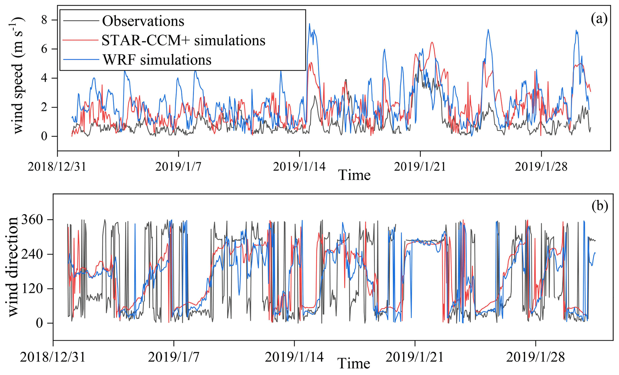
Figure 4Evaluation of the wind simulation results at the BSC monitoring site (see in Fig. 3a): the simulated (by the WRF (blue line) and STAR-CCM+ (red line) models) and the observed (grey line) hourly near-surface wind speeds (a) and wind directions (b).
3.2 The characteristics of the street-level wind fields
In urban areas, the complex spatial structure and layout of buildings have a great influence on the street-level wind field (Liu et al., 2018; Park et al., 2015), which is a crucial meteorological factor that controls the transport of air pollutants. The street-level wind field characteristics were simulated by the S-TRACK and discussed comprehensively in this paper for the overall average in January as well as for different background wind directions, i.e. north, south, west and east.
3.2.1 The average wind field characteristics
Figure 5a and b illustrate the distribution of the average wind streamlines in January at the height of 5 and 40 m, respectively. At the height of 5 m, the wind field structure is more complicated (Fig. 5a) than that at 40 m (Fig. 5b). The wind speed is relatively more intense in the areas where the buildings are sparse and smaller. In addition, the flow fields diverge or converge due to the layout of buildings and streets, causing the wind direction inside blocks to differ from the background wind direction greatly. As the density of buildings gradually decreases with the increases in height, this phenomenon diminishes, reflected by the relatively more consistent wind fields at 40 m (Fig. 5b). The phenomenon was also found in a previous study (Sui et al., 2016).
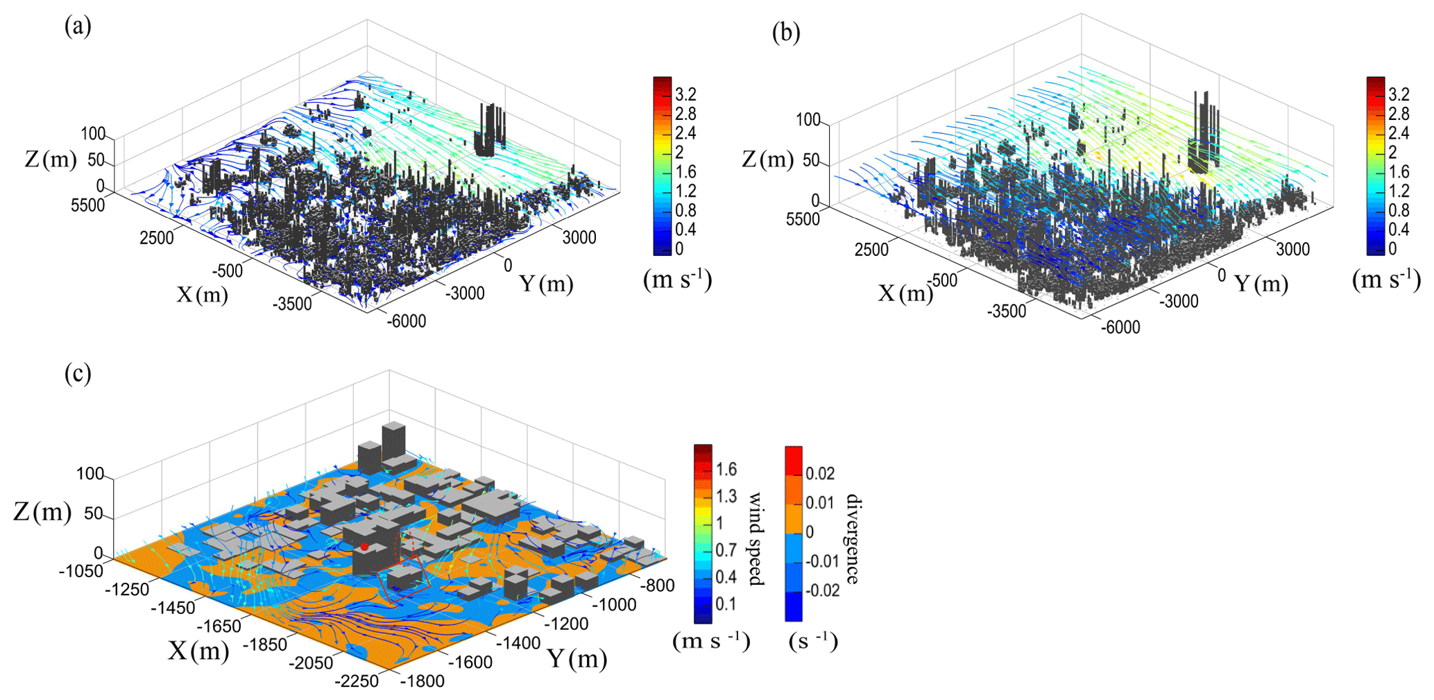
Figure 5The simulated wind streamlines at the height of 5 (a) and 40 m (b) averaged in January 2019 in the whole S-TRACK simulation domain; the simulated wind streamlines and divergence (c) at the near surface averaged in January 2019 in the sub-domain A (see in Fig. 3a). The BSC monitoring site is marked with red dot.
To clearly show the details of the wind field, sub-domain A (Fig. 3a) with complex building structures is selected from the entire computational domain. The near-surface winds disperse or converge horizontally and rise or subside vertically with the building (Fig. 5c). During the climb or fall with the building, downwash winds with high wind speeds occur (as shown in the red dashed circles). Due to the complexity of the building layout, local circulation is formed on the west side of the BSC monitoring site, making the airflow around the building on the south side of the station accumulate and form an obvious convergence area (Fig. 5c), which is not conducive to the air circulation and pollution transport (as shown in the red box).
3.2.2 The wind field characteristics under different background wind directions
Figure 6 shows the distributions of near-surface wind and its divergence under four different background wind directions. In general, the overall wind direction in the area is consistent with the background wind direction, but the airflow near the surface is significantly affected by the building layout, thus forming local circulations with divergence or convergence zones. The wind speeds in the areas with dense buildings are significantly smaller than those in open areas (Fig. 6a-1, b-1, c-1, and d-1), which is attributed to the obvious frictional dragging effect of the dense buildings. The overall wind direction in the area is generally the same as the background wind direction, but the airflow is diverged or converged by the influence of the building layout, resulting in a great difference in wind direction inside the block from the background. When the background wind direction is north or west (Fig. 6b and c), the overall wind speed in the area is relatively large. This is mainly due to the temperate monsoon climate in Zhengzhou, where northwest and west winds prevail in winter and wind speeds are relatively high.
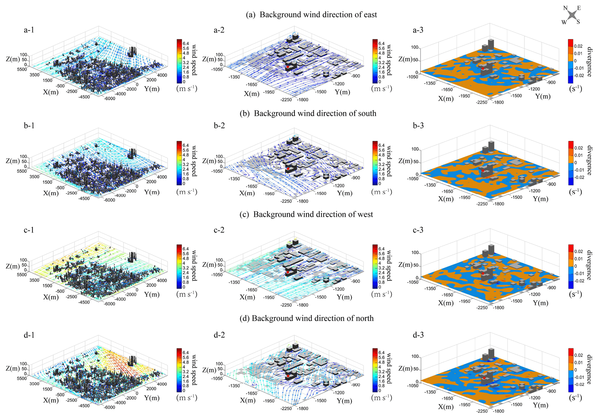
Figure 6The wind field streamlines and divergences under the background wind directions of east (a), south (b), west (c), and north (d). The BSC monitoring site is marked with a red dot.
It is found that the windward side of the building is mostly a divergence zone, and the leeward side is mainly a convergence zone, which is more obvious for higher buildings. When the airflow meets the building, the airflow on the windward side of the building is blocked and thus spreads outward, forming a divergence zone. The airflow on the leeward side of the building converges and generates a vortex with lower wind speed, forming a convergence zone. For example, at the BSC monitoring site, when the background wind direction is west, the wind speed on the windward side of the building is higher and diffused outward by the building blockage (Fig. 6c-2), resulting in a significant divergence zone (Fig. 6c-3). High-rise buildings have a greater impact on the wind field and cause a strong degree of convergence and divergence. It can be seen that the degree of divergence or convergence around the high-rise building is more significant than those around low buildings in the area (Fig. 6b-3, c-3, and d-3). In addition, the ventilation is better when the dominant airflow is in the same direction as building layout (Fig. 6c). In the process of urban construction, the influence of prevailing wind direction on the layout of buildings should be considered, which could effectively improve the efficiency of urban ventilation.
3.3 Potential contribution of traffic sources
In this section, the S-TRACK system is used to analyse the potential contribution of main traffic roads (R1–R4) in sub-domain B (Fig. 3a) to several receptor sites nearby with different heights and locations with a number of schools and residential areas. The widths of roads R1–R4 are about 45, 33, 20, and 18 m, respectively. Since detailed information on road traffic emissions was not available, the road traffic emissions were assumed to be uniformly distributed and with identical intensity in this study. During the backward-trajectory simulation, as long as the particles passed within 5 m in height above the road, they are considered to be a potential contribution from the road emissions to the receptor site. Additionally, the potential contribution of traffic source under different background wind directions was also explored. The residence-time analysis (RTA), which has been previously used to identify the accounted for contribution of emission sources to air quality of receptors (Ashbaugh et al., 1985; Hopke et al., 2005; Poirot et al., 2001; Salvador et al., 2008; Yu, 2017), was selected in this study to assess the potential contribution ratio (PCR) of the traffic source for receptors. The RTA is expressed as
where Ri,j indicates the contribution ratio of the grid (i,j) to receptor, τi,j means the residence time in the grid (i,j), and t means the total residence time in all grid cells.
3.3.1 Potential contribution of traffic sources at different sites in winter
In order to analyse the potential contribution of the traffic source to different locations, the receptor sites were selected at different locations and heights, and the overall PCR of all wind directions for January 2019 was calculated by RTA (Table 4). Receptor sites S2–S8, with an identical horizontal location but different heights, are selected to investigate contributions of traffic sources to receptor sites at different heights. The PCR of all four roads are 4.05 %, 4.25 %, 4.33 %, and 4.67 % for receptor sites S2 to S5, with heights of 2, 5, 10, and 15 m, respectively. However, as the receptor height continues to rise, namely from S5 to S8, the PCR of the roads gradually decreases from 4.67 % to 3.55 % (Table 4). It is noteworthy that the contributions from R1 and R3 are primary, especially R1, which may be due to the closer distance to the site and the generally northeast wind field. The potential contribution of the traffic source is the greatest when the receptor site is located at a height of 15 m, suggesting the air quality at that height is most susceptible to traffic emissions under the northeast wind field. In addition, according to density distribution (refers to the number of particles that have stayed in the space of 10 m×10 m in the horizontal direction and 5 m from the surface to above in the vertical direction) of all trajectory points that have passed through the traffic roads (Fig. 7), it can be seen that the road section with a large potential contribution to the receptor sites is generally located to their northeast, which might be a result of the combination effect of the background wind field and the building layout. For more details, the vertical structure of winds along the direction of the wind field at the receptor site S2 (Fig. 8b) is also presented. It can be seen that there is a general upward motion in the airflow, showing the position with the greatest PCR from traffic sources is located at a certain height, which is about 15 m over the receptor site S2 in this case.
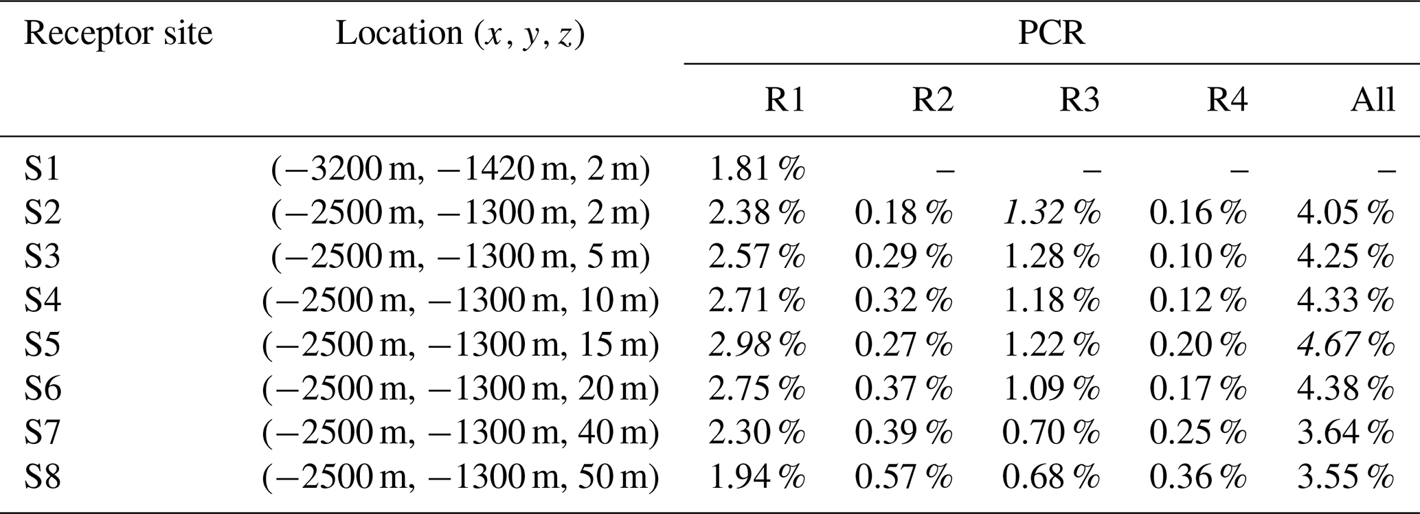
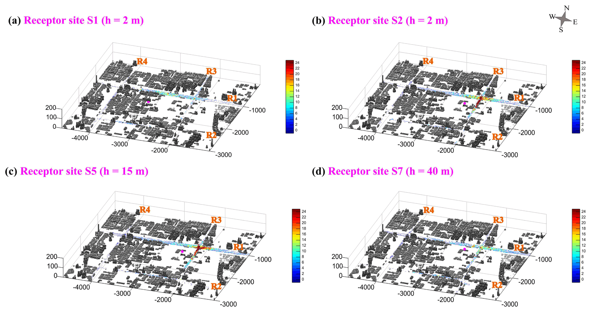
Figure 7Density distribution on the road of backward trajectory particles released from different receptor sites (S1, S2, S5, and S7; see details in Table 4). The four receptor sites are all marked with magenta dots.
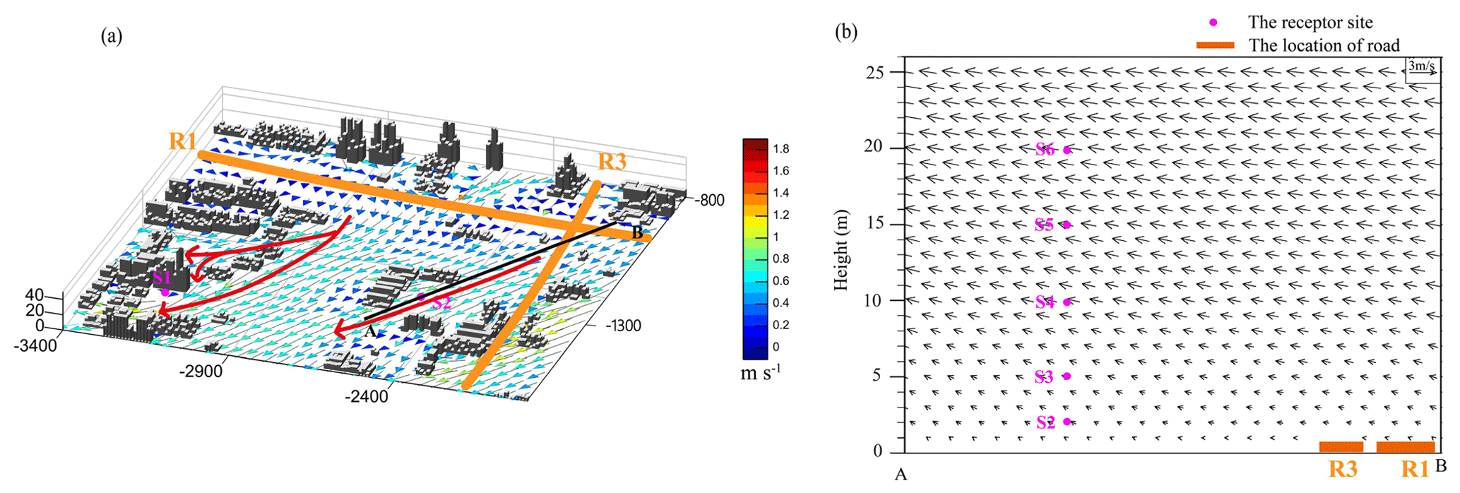
Figure 8The (a) average surface wind and (b) vertical structure of average winds along the wind direction around the receptor site S2 (line AB) in January 2019. The road R1 is marked with an orange line, the location of the vertical profile is shown as a black line, and the receptor sites S1 to S6 are all marked with magenta dots.
It can be seen from Table 4 that R1 is the road with the greatest potential contribution to the receptor sites. The horizontal distance between road R1 and the receptor sites is about 300 m, and the peak of the PCR occurs at a height of about 15 m (corresponding to the site S5). However, for the road R3, which is closest to the receptor sites in the horizontal (about 200 m), the contribution ratios are lower than those of the road R1. Figure 8a shows that the near-ground winds are generally northeast, resulting in the probability of traffic contributions from R1 and R3 road sections upwind of the site S2 being roughly the same. Nonetheless, as mentioned in Sect. 3.3, the width for the road R1 is about twice that of the road R3. Therefore, even though R1 was a little farther from the receptor sites than R3, the contribution ratios of R1 to the sites were calculated to be larger than those of R3. For R2 and R4, the distance from the receptor sites is about 1200 and 1500 m, respectively, farther away than those of R1 and R3. In addition, under northeast winds, the traffic source was hardly transported to the receptor sites, rendering the contribution ratios quite small below 50 m (Table 4). It can also be seen, from Table 4, that the corresponding PCR of R2 and R4 may peak at a height over 50 m.
Since the road R1 had the largest potential contribution to the receptor sites, the contribution of R1 to different positions is focused in the subsequent discussion. For the receptor site S1, which is about 400 m from R1, located in a dense building area with the building height at 30 to 40 m, the PCR of the traffic source to the receptor site is calculated to be 1.81 %. For the receptor site S2, which is about 300 m from the traffic road, located in an open area and surrounded by low buildings, the PCR of the traffic source is determined to be 2.38 %. It might be inferred that the wind field difference partially resulted from the influence of building layout and led to the higher contribution ratio to S2. From the average wind field in January 2019 (Fig. 8a), it can be seen that the winds were influenced by high-rise buildings around S1, resulting in a change in transport path of pollutants and thus making it difficult for pollutants to reach the S1 site. However, for the S2 site, the winds were less influenced by the buildings, and pollutants were more easily transported there.
3.3.2 Potential contribution of traffic sources under different background wind directions
In order to investigate the potential contribution of traffic sources under different background wind directions, the receptor site S2 influenced by R1 under the east, the south, the west, and the north wind directions was classified from the simulation period. The PCRs of the traffic source were estimated to be 2.45 %, 0.07 %, 1.98 %, and 2.97 % for the east, the south, the west, and the north wind directions, respectively, revealing that the difference in potential contribution was largest between the south and north wind directions. When the background wind direction was south, the receptor site was located upwind of the road, and the road traffic source contributed very little to the receptor site. On the contrary, when the receptor site was downwind of the road with northern winds, the contribution ratio of road traffic source to the receptor site was the greatest. When the background wind direction was east and west, the contribution ratio to the receptor point was similar, ranging between the ratios under the south and north wind directions. The lower contribution ratio during westerly winds relative to that under easterly winds might partially be due to the denser distribution of buildings upwind of the receptor site. Complex building layouts changed the structure of the wind field and thus had an impact on the transport of pollutants. The slow air circulation in dense building areas made it unfavourable for pollutants to be transported. In the windward side of the dense building area, the wind was blocked and diverted to both sides of the building. Pollutants were difficult to transport to the leeward side of the building, where the receptor site was located. The results of the potential contribution of traffic sources under different background wind conditions are helpful to understand the street-level pollution transport characteristics and provide effective suggestions for the traffic pollution control strategies.
A street-level pollutant tracking system has been developed to simulate micro-scale meteorology and used to analyse the characteristics of wind environment and the potential traffic source contribution of air pollution to receptors through backward simulations in a city district. In general, the S-TRACK system is effective in simulating street-level meteorological and pollution problems. The presence of buildings has a significant effect on the wind environment; i.e. the dragging effect of dense buildings renders the wind speed inside the block smaller than the background wind speed. The ventilation is better when the dominant airflow is consistent with the direction of building layout. Influenced by the building layout, the airflow near the surface is formed with divergence and convergence zones. The windward side of the building is mostly a divergence zone, and the leeward side is mostly a convergence zone, which is more obvious for higher buildings.
As a test case, the S-TRACK system has been used to investigate the potential contribution of traffic sources to receptor sites with different locations, heights, and background wind directions in a city district. For a specific location of this case study, the potential traffic contribution ratios also varied with height at about 4.05 %, 4.25 %, 4.33 %, 4.67 %, 4.38 %, 3.64 %, and 3.55 % for 2, 5, 10, 15, 20, 40, and 50 m, respectively, manifesting a significant trend of increasing and then decreasing with height. In addition, the height of position with the greatest PCR from the traffic source varies jointly, influenced by the distance between the position and traffic source, as well as the background wind field. The potential contribution of traffic sources to a specific receptor site varies under different background wind directions, which are estimated to be 2.45 %, 0.07 %, 1.98 %, and 2.97 % for the east, the south, the west, and the north wind directions, respectively. The difference in potential contribution under east and west wind directions might partially be due to the density of buildings upwind of the receptor site.
In the future, in-depth simulation experiments with different building layouts, wind field environments, and distances between traffic source and receptor are required to quantify the potential contribution of street-level pollution sources and to establish the relationship between meteorological conditions, buildings, and various emissions (point, area, and line sources) in the street level for an effective management of regional pollution in a city.
A1 Some settings to improve the calculation efficiency of CFD
It is true that using a CFD model for the atmospheric numerical simulation has the problem of high computational cost. In this study, RANS equations are chosen as the CFD model, which requires a relatively small amount of computational resources. The time step of STAR-CCM+ is set to 60 s, with a maximum of 20 internal iterations in each time step, and a parallel computing with 32 CPUs is done on a supercomputer. The simulation error increases with the simulation time. In order to ensure the efficiency and accuracy of the simulation, the month was divided into four time periods to simulate, as shown in Table A1.
Table A1The division of each simulation time period and the physical time spent on the simulation.
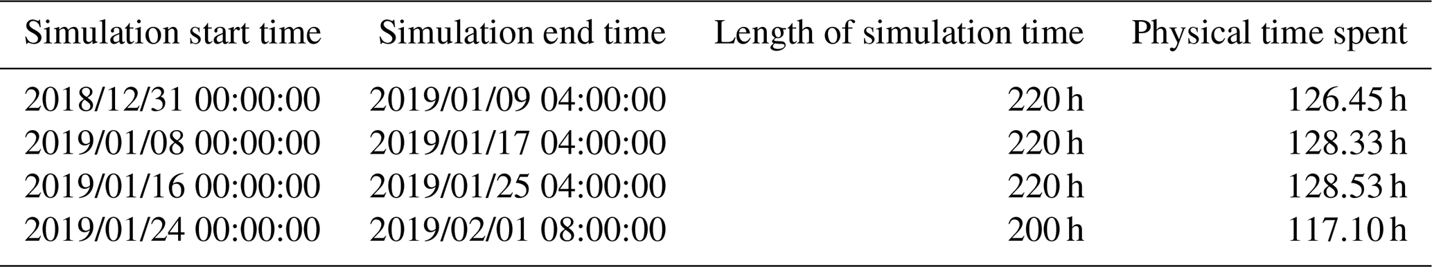
Table A2The location of each meteorological station and the average wind speed.
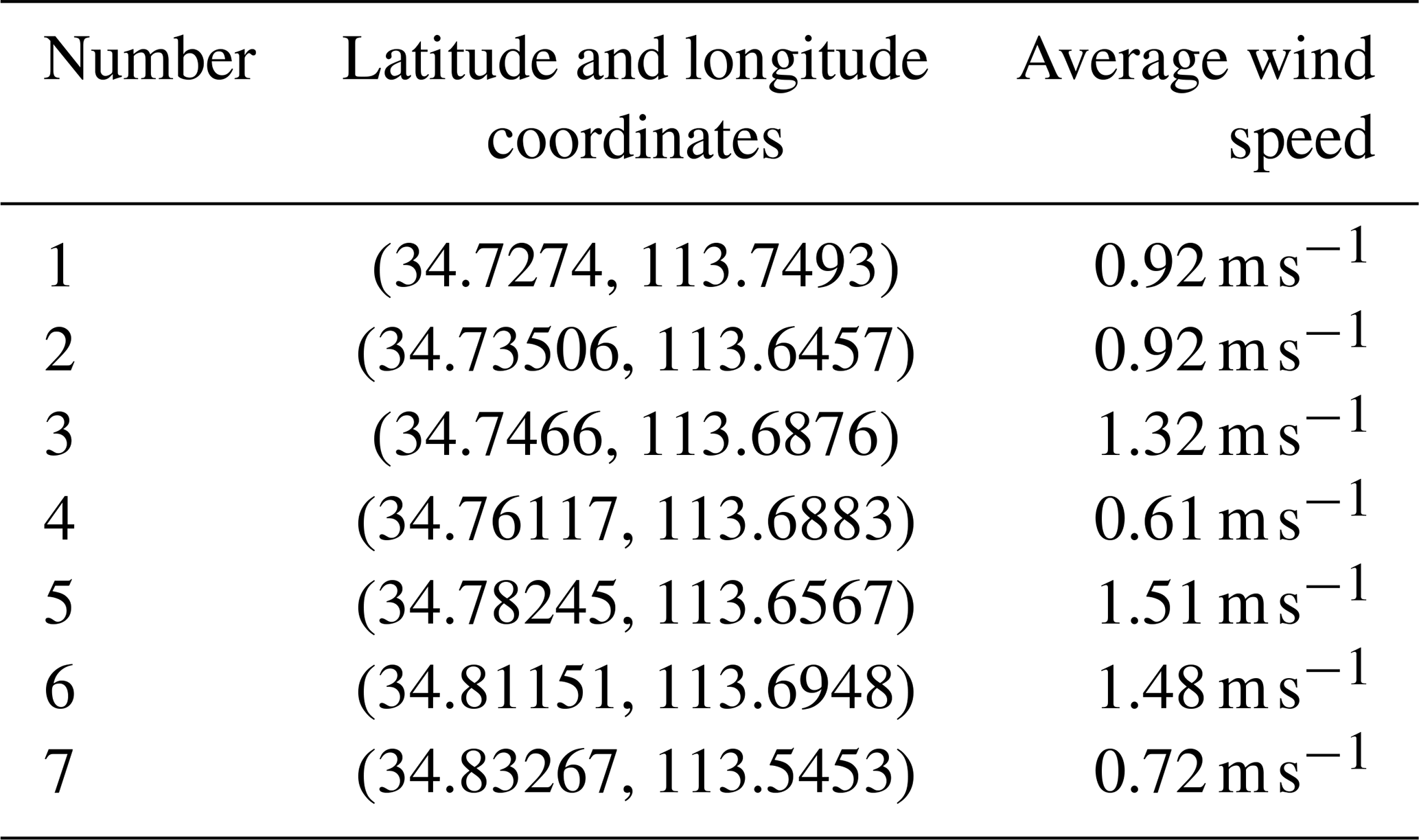
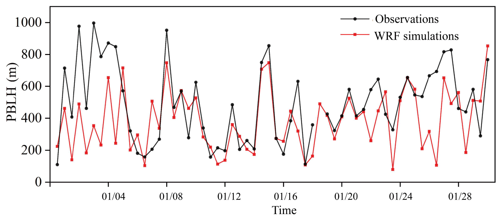
Figure A1Time series of the observed (black) and simulated (red) PBLH at 08:00 and 20:00 Beijing time (BJT) at the Zhengzhou sounding site.
A2 Significance test
A significance test is used to determine the significance of the results in relation to the null hypothesis, with a p value, or probability value, describing how likely the data would have occurred by random chance (i.e. that the null hypothesis is true). A p value less than 0.05 (typically ≤0.05) is statistically significant. It indicates strong evidence against the null hypothesis, as there is less than a 5 % probability the null is correct.
A3 The observed data for January 2019 at various meteorological stations in Zhengzhou city
A4 Hit rates
The hit rate is a reliable overall measure for describing model performance.
where m is the number of comparison data, and A is to consider the desired model accuracy. The single hit rate is calculated ranging from 100 % if all model results are within A of the observations to 0 % if none are.
A5 Divergence
The divergence is a quantity that describes the degree to which air converges from its surroundings to a point or flows away from a point. It is used to describe the intensity of divergence and convergence at locations in space. The formula is as follows.
where u, v, and w are the components of the wind in the x, y, and z directions, respectively. When the divv<0, the location is convergence; when the divv>0, the location is divergence.
A6 PBLH validation
The bulk Richardson number (Ri) method was taken to estimate the PBLH based on the sounding data of Zhengzhou. Ri is expressed as
where z is the height above ground, s the surface, g the acceleration of gravity, θv the virtual potential temperature, u and v the components of wind speed, and u∗ the surface friction velocity. u∗ can be ignored here due to it being small relative to the wind shear (Vogelezang and Holtslag, 1996). Previous theoretical and laboratory studies suggested that when Ri is smaller than a critical value (∼0.25), the laminar flow becomes unstable (Stull, 1988). Therefore, the lowest level z at which the interpolated Ri exceeds the critical value of 0.25 is referred to as PBLH in this study, which is referred to as the criterion used by Seidel et al. (2012). The R value is 0.57, passing the 99 % significance test. It can be seen from Fig. A1 that the variation in boundary layer height is generally captured.
All source code and data can be accessed by contacting the corresponding authors Sunling Gong (gongsl@cma.gov.cn) and Lei Zhang (leiz09@cma.gov.cn).
SG and LZ designed the research. HZ performed the simulations and wrote the manuscript with suggestions from all authors. JM, HK, XW, and SL assisted with data processing. JH, YW, JN, and LS participated in the scientific interpretation and discussion. All authors contributed to the discussion and improvement of the paper.
The contact author has declared that neither they nor their co-authors have any competing interests.
Publisher's note: Copernicus Publications remains neutral with regard to jurisdictional claims in published maps and institutional affiliations.
This article is part of the special issue “Air quality research at street level (ACP/GMD inter-journal SI)”. It is not associated with a conference.
The authors would like to acknowledge Bin Cui and Lin Zhang from the Peking University and Liangfu Chen from Chinese Academy of Sciences for their valuable suggestions to improve the article.
This research has been supported by the National Natural Science Foundation of China (grant nos. 91744209, 41975131, and 41705080), the CAMS Basis Research Project (grant no. 2019Z009), CAMS Science and Technology Development Fund (grant no. 2018KJ020), and the Atmospheric special integration project (grant no. 2019YFC0214801).
This paper was edited by Yang Zhang and reviewed by Sergio Ibarra and one anonymous referee.
Ashbaugh, L., Malm, W., and Sadeh, W.: A residence time probability analysis of sulfur concentrations at grand Canyon national park, Atmos. Environ., 19, 1263–1270, https://doi.org/10.1016/0004-6981(85)90256-2, 1985.
Aynsley, R.: Politics of pedestrian level urban wind control, Build. Environ., 24, 291–295, https://doi.org/10.1016/0360-1323(89)90022-X, 1989.
Borge, R., Santiago, J. L., de la Paz, D., Martín, F., Domingo, J., Valdés, C., Sánchez, B., Rivas, E., Rozas, M. T., Olaechea Lázaro, S., Pérez, J., and Fernández, Á.: Application of a short term air quality action plan in Madrid (Spain) under a high-pollution episode – Part II: Assessment from multi-scale modelling, Sci. Total Environ., 635, 1574–1584, https://doi.org/10.1016/j.scitotenv.2018.04.323, 2018.
Brioude, J., Arnold, D., Stohl, A., Cassiani, M., Morton, D., Seibert, P., Angevine, W., Evan, S., Dingwell, A., Fast, J. D., Easter, R. C., Pisso, I., Burkhart, J., and Wotawa, G.: The Lagrangian particle dispersion model FLEXPART-WRF version 3.1, Geosci. Model Dev., 6, 1889–1904, https://doi.org/10.5194/gmd-6-1889-2013, 2013.
Carvalho, D., Rocha, A., Gómez-Gesteira, M., and Santos, C.: A sensitivity study of the WRF model in wind simulation for an area of high wind energy, Environ. Modell. Softw., 33, 23–34, https://doi.org/10.1016/j.envsoft.2012.01.019, 2012.
Cécé, R., Bernard, D., Brioude, J., and Zahibo, N.: Microscale anthropogenic pollution modelling in a small tropical island during weak trade winds: Lagrangian particle dispersion simulations using real nested LES meteorological fields, Atmos. Environ., 139, 98–112, https://doi.org/10.1016/j.atmosenv.2016.05.028, 2016.
Chen, F. and Dudhia, J.: Coupling an Advanced Land Surface–Hydrology Model with the Penn State–NCAR MM5 Modeling System. Part I: Model Implementation and Sensitivity, Mon. Weather Rev., 129, 569–585, https://doi.org/10.1175/1520-0493(2001)129<0569:CAALSH>2.0.CO;2, 2001.
de Foy, B., Burton, S. P., Ferrare, R. A., Hostetler, C. A., Hair, J. W., Wiedinmyer, C., and Molina, L. T.: Aerosol plume transport and transformation in high spectral resolution lidar measurements and WRF-Flexpart simulations during the MILAGRO Field Campaign, Atmos. Chem. Phys., 11, 3543–3563, https://doi.org/10.5194/acp-11-3543-2011, 2011.
Ehrhard, J., Khatib, I., Winkler, C., Kunz, R., Moussiopoulos, N., and Ernst, G.: The microscale model MIMO: development and assessment, J. Wind Eng. Ind. Aerod., 85, 163–176, https://doi.org/10.1016/S0167-6105(99)00137-3, 2000.
Fast, J. D. and Easter, R. C.: A Lagrangian Particle Disper-sion Model Compatible with WRF, in 7th Annual WRFUser's Workshop, 19–22 June 2006, Boulder, CO, USA, P6.2, http://www2.mmm.ucar.edu/wrf/users/workshops/WS2006/abstracts/PSession06/P6_02_Fast.pdf (last access: 29 July 2021), 2006.
Fernando, H., Zajic, D., Sabatino, S. D., Dimitrova, R., and Dallman, A.: Flow, turbulence, and pollutant dispersion in urban atmosphere, Phys. Fluids, 22, 051301, https://doi.org/10.1063/1.3407662, 2010.
Gao, Y., Shan, H., Zhang, S., Sheng, L., Li, J., Zhang, J., Ma, M., Meng, H., Luo, K., Gao, H., and Yao, X.: Characteristics and sources of PM2.5 with focus on two severe pollution events in a coastal city of Qingdao, China, Chemosphere, 247, 125861, https://doi.org/10.1016/j.chemosphere.2020.125861, 2020.
Gosman, A. D.: Developments in CFD for industrial and environmental applications in wind engineering, J. Wind Eng. Ind. Aerod., 81, 21–39, https://doi.org/10.1016/S0167-6105(99)00007-0, 1999.
He, J., Mao, H., Gong, S., Yu, Y., and Zou, C.: Investigation of particulate matter regional transport in Beijing based on numerical simulation, Aerosol Air Qual. Res., 17, 1181–1189, https://doi.org/10.4209/AAQR.2016.03.0110, 2017.
He, J., Zhang, L., Yao, Z., Che, H., Gong, S., Wang, M., Zhao, M., and Jing, B.: Source apportionment of particulate matter based on numerical simulation during a severe pollution period in Tangshan, North China, Environ. Pollut., 266, 115133, https://doi.org/10.1016/j.envpol.2020.115133, 2020.
He, J. J., Yu, Y., Liu, N., Zhao, S. P., and Chen, J. B.: Impact of land surface information on WRFs performance in complex terrain area, Chin. J. Atmos. Sci., 38, 484–498, https://doi.org/10.3878/j.issn.1006-9895.2013.13186, 2014.
He, J. J., Yu, Y., Yu, L. J., Liu, N., and Zhao, S. P.: Impacts of uncertainty in land surface information on simulated surface temperature and precipitation over China, Int. J. Climatol., 37, 829–847, https://doi.org/10.1002/joc.5041, 2017.
Hendricks, E. A., Diehl, S. R., Burrows, D. A., and Keith, R.: Evaluation of a Fast-Running Urban Dispersion Modeling System Using Joint Urban 2003 Field Data, J. Appl. Meteorol. Clim., 46, 2165–2179, https://doi.org/10.1175/2006JAMC1289.1, 2007.
Heo, J., Foy, B. D., Olson, M. R., Pakbin, P., Sioutas, C., and Schauer, J.: Impact of regional transport on the anthropogenic and biogenic secondary organic aerosols in the Los Angeles Basin, Atmos. Environ., 103, 171–179, https://doi.org/10.1016/J.ATMOSENV.2014.12.041, 2015.
Hopke, P., Zhou, L., and Poirot, R.: Reconciling trajectory ensemble receptor model results with emissions, Environ. Sci. Technol., 39, 7980–7983, https://doi.org/10.1021/es049816g, 2005.
Iacono, M. J., Delamere, J. S., Mlawer, E. J., Shephard, M. W., and Collins, W. D.: Radiative Forcing by Long-Lived Greenhouse Gases: Calculations with the AER Radiative Transfer Models, J. Geophys. Res.-Atmos., 113, D13103, https://doi.org/10.1029/2008JD009944, 2008.
Kochanski, A. K., Pardyjak, E. R., Stoll, R., Gowardhan, A., Brown, M. J., and Steenburgh, W. J.: One-Way Coupling of the WRF-QUIC Urban Dispersion Modeling System, J. Appl. Meteorol. Clim., 54, 2119–2139, https://doi.org/10.1175/JAMC-D-15-0020.1, 2015.
Kurppa, M., Hellsten, A., Auvinen, M., Raasch, S., Vesala, T., and Järvi, L.: Ventilation and Air Quality in City Blocks Using Large-Eddy Simulation – Urban Planning Perspective, Atmosphere, 9, 65, https://doi.org/10.3390/ATMOS9020065, 2018.
Kwak, K.-H., Baik, J.-J., Ryu, Y.-H., and Lee, S.-H.: Urban air quality simulation in a high-rise building area using a CFD model coupled with mesoscale meteorological and chemistry-transport models, Atmos. Environ., 100, 167–177, https://doi.org/10.1016/j.atmosenv.2014.10.059, 2015.
Lei, L., Fei, H., Cheng, X. L., and Han, H. Y.: The application of computational fluid dynamics to pedestrian level wind safety problem induced by high-rise buildings, Chin. Phys. B, 13, 1070–1075, https://doi.org/10.1088/1009-1963/13/7/018, 2004.
Lei, L. I., Yang, L., Zhang, L. J., and Jiang, Y.: Numerical Study on the Impact of Ground Heating and Ambient Wind Speed on Flow Fields in Street Canyons, Adv. Atmos. Sci., 29, 1227–1237, https://doi.org/10.1007/s00376-012-1066-3, 2012.
Li, L., Hu, F., Cheng, X. L., Jiang, J. H., and Ma, X. G.: Numerical simulation of the flow within and over an intersection model with Reynolds-averaged Navier-Stokes method, Chin. Phys. B, 15, 149–155, https://doi.org/10.1088/1009-1963/15/1/024, 2006.
Li, S., Sun, X., Zhang, S., Zhao, S., and Zhang, R.: A Study on Microscale Wind Simulations with a Coupled WRF–CFD Model in the Chongli Mountain Region of Hebei Province, China, Atmosphere, 10, 731, https://doi.org/10.3390/atmos10120731, 2019.
Li, X.-X., Liu, C.-H., and Leung, D. Y. C.: Large-Eddy Simulation of Flow and Pollutant Dispersion in High-Aspect-Ratio Urban Street Canyons with Wall Model, Bound.-Lay. Meteorol., 129, 249–268, https://doi.org/10.1007/s10546-008-9313-y, 2008.
Lin, Y. L., Farley, R. D., and Orville, H. D.: Bulk Parameterization of the Snow Field in a Cloud Model, J. Appl. Meteorol., 22, 1065–1092, https://doi.org/10.1175/1520-0450(1983)022<1065:BPOTSF>2.0.CO;2, 1983.
Liu, N., Yu, Y., He, J., and Zhao, S.: Integrated modeling of urban-scale pollutant transport: application in a semi-arid urban valley, Northwestern China (SCI), Atmos. Pollut. Res., 4, 306–314, https://doi.org/10.5094/APR.2013.034, 2013.
Liu, S., Pan, W., Zhao, X., Zhang, H., Cheng, X., Long, Z., and Chen, Q.: Influence of surrounding buildings on wind flow around a building predicted by CFD simulations, Build. Environ., 140, 1–10, https://doi.org/10.1016/j.buildenv.2018.05.011, 2018.
Macdonald, R. W., Griffiths, R. F., and Cheah, S. C.: Field experiments of dispersion through regular arrays of cubic structures, Atmos. Environ., 31, 783–795, https://doi.org/10.1016/S1352-2310(96)00263-4, 1997.
Madala, S., Satyanarayana, A. N., Srinivas, C., and Kumar, M.: Mesoscale atmospheric flow-field simulations for air quality modeling over complex terrain region of Ranchi in eastern India using WRF, Atmos. Environ., 107, 315–328, https://doi.org/10.1016/J.ATMOSENV.2015.02.059, 2015.
Mavroidis, I., Griffiths, R. F., and Hall, D. J.: Field and wind tunnel investigations of plume dispersion around single surface obstacles, Atmos. Environ., 37, 2903–2918, https://doi.org/10.1016/S1352-2310(03)00300-5, 2003.
Miao, Y. C., Liu, S. H., Zheng, H., Zheng, Y. J., Chen, B. C., and Wang, S.: A multi-scale urban atmospheric dispersion model for emergency management, Adv. Atmos. Sci., 31, 13, https://doi.org/10.1007/s00376-014-3254-9, 2014.
Milliez, M. and Carissimo, B.: Computational Fluid Dynamical Modelling of Concentration Fluctuations in an Idealized Urban Area, Bound.-Lay. Meteorol., 127, 241–259, https://doi.org/10.1007/s10546-008-9266-1, 2008.
Nakanishi, M. and Niino, H.: An Improved Mellor–Yamada Level-3 Model: Its Numerical Stability and Application to a Regional Prediction of Advection Fog, Bound.-Lay. Meteorol., 119, 397–407, https://doi.org/10.1007/S10546-005-9030-8, 2006.
Nelson, M. A., Brown, M. J., Halverson, S. A., Bieringer, P. E., Annunzio, A., Bieberbach, G., and Meech, S.: A Case Study of the Weather Research and Forecasting Model Applied to the Joint Urban 2003 Tracer Field Experiment. Part 2: Gas Tracer Dispersion, Bound.-Lay. Meteorol., 161, 461–490, https://doi.org/10.1007/s10546-016-0188-z, 2016.
Park, S. B., Baik, J. J., and Han, B. S.: Large-eddy simulation of turbulent flow in a densely built-up urban area, Environ. Fluid Mech., 15, 235–250, https://doi.org/10.1007/s10652-013-9306-3, 2015.
Poirot, R., Wishinski, P., Hopke, P., and Polissar, A.: Comparative application of multiple receptor methods to identify aerosol sources in northern Vermont, Environ. Sci. Technol., 35, 4622–4636, https://doi.org/10.1021/es011442t, 2001.
Sada, K. and Sato, A.: Numerical calculation of flow and stack-gas concentration fluctuation around a cubical building, Atmos. Environ., 36, 5527–5534, https://doi.org/10.1016/S1352-2310(02)00668-4, 2002.
Salvador, P., Artíñano, B., Querol, X., and Alastuey, A.: A combined analysis of backward trajectories and aerosol chemistry to characterise long-range transport episodes of particulate matter: the madrid air basin, a case study, Sci. Total Environ., 390, 495–506, https://doi.org/10.1016/j.scitotenv.2007.10.052, 2008.
Sandeepan, B., Rakesh, P. T., and Venkatesan, R.: Numerical simulation of observed submesoscale plume meandering under nocturnal drainage flow, Atmos. Environ., 69, 29–36, https://doi.org/10.1016/J.ATMOSENV.2012.12.007, 2013.
Santiago, J. L., Borge, R., Martín, F., de la Paz, D., Martilli, A., Lumbreras, J., and Sanchez, B.: Evaluation of a CFD-based approach to estimate pollutant distribution within a real urban canopy by means of passive samplers, Sci. Total Environ., 576, 46–58, https://doi.org/10.1016/j.scitotenv.2016.09.234, 2017.
Santiago, J. L., Sanchez, B., Quaassdorff, C., de la Paz, D., Martilli, A., Martín, F., Borge, R., Rivas, E., Gómez-Moreno, F. J., Díaz, E., Artiñano, B., Yagüe, C., Vardoulakis, S.: Performance evaluation of a multiscale modelling system applied to particulate matter dispersion in a real traffic hot spot in Madrid (Spain) – ScienceDirect, Atmos. Pollut. Res., 11, 141–155, https://doi.org/10.1016/j.apr.2019.10.001, 2020.
Schlünzen, K. H. and Sokhi, R. S.: Overview of Tools and Methods for Meteorological and Air Pollution Mesoscale Model Evaluation and User Training, Joint report by WMO and COST 728, WMO/TD-No. 1457, Geneva, Switzerland, ISBN 978-1-905313-59-4, 2008.
Seidel, D. J., Zhang, Y., Beljaars, A., Golaz, J. C., Jacobson, A. R., and Medeiros, B.: Climatology of the planetary boundary layer over the continental United States and Europe, J. Geophys. Res.-Atmos., 117, D17106, https://doi.org/10.1029/2012JD018143, 2012.
Stam, J.: Stable fluids. In Proceedings of the 26th annual conference on Computer graphics and interactive techniques (SIGGRAPH '99), ACM Press/Addison-Wesley Publishing Co., USA, 121–128, https://doi.org/10.1145/311535.311548, 1999.
Stohl, A.: A backward modeling study of intercontinental pollution transport using aircraft measurements, J. Geophys. Res., 108, 4370, https://doi.org/10.1029/2002jd002862, 2003.
Stohl, A., Forster, C., Frank, A., Seibert, P., and Wotawa, G.: Technical note: The Lagrangian particle dispersion model FLEXPART version 6.2, Atmos. Chem. Phys., 5, 2461–2474, https://doi.org/10.5194/acp-5-2461-2005, 2005.
Stull, R. B.: An Introduction to Boundary Layer Meteorology, Springer Netherlands, Dordrecht, ISBN 978-94-009-3027-8, 1988.
Sui, L., Jiang, M., Li, Z., and Zhou, S.: Diffusion effect analysis of pollution gas under the impact of urban three-dimensional pattern, in: 5th International Conference on Energy and Environmental Protection, Shengzhen, China, 17–18 September 2016, 903–909, https://doi.org/10.2991/iceep-16.2016.158, 2016.
Temimi, M., Fonseca, R., Reddy, N. N., Weston, M., and Naqbi, H. A.: Assessing The Impact of Changes in Land Surface Conditions on WRF Predictions in Arid Regions, J. Hydrometeorol., 21, 2829–2853, https://doi.org/10.1175/JHM-D-20-0083.1, 2020.
Tewari, M., Kusaka, H., Chen, F., Coirier, W. J., Kim, S., Wyszogrodzki, A. A., and Warner, T. T.: Impact of coupling a microscale computational fluid dynamics model with a mesoscale model on urban scale contaminant transport and dispersion, Atmos. Res., 96, 656–664, https://doi.org/10.1016/j.atmosres.2010.01.006, 2010.
Vogelezang, D. and Holtslag, A.: Evaluation and model impacts of alternative boundary-layer height formulations, Bound.-Lay. Meteorol., 81, 245–269, https://doi.org/10.1007/BF02430331, 1996.
Yu, C., Zhao, T., Bai, Y., Zhang, L., Kong, S., Yu, X., He, J., Cui, C., Yang, J., You, Y., Ma, G., Wu, M., and Chang, J.: Heavy air pollution with a unique “non-stagnant” atmospheric boundary layer in the Yangtze River middle basin aggravated by regional transport of PM2.5 over China, Atmos. Chem. Phys., 20, 7217–7230, https://doi.org/10.5194/acp-20-7217-2020, 2020.
Yu, T. Y.: Source identification of emission sources for hydrocarbon with backward trajectory model and statistical methods, Pol. J. Environ. Stud., 26, 893–902, https://doi.org/10.15244/pjoes/65744, 2017.
Zhang, H., Xu, T., Zong, Y., Tang, H., Liu, X., and Wang, Y.: Influence of Meteorological Conditions on Pollutant Dispersion in Street Canyon, Procedia Engineer., 121, 899–905, https://doi.org/10.1016/J.PROENG.2015.09.047, 2015.
Zhang, H., Tang, S., Yue, H., Wu, K., Zhu, Y., Liu, C.-J., Liang, B., and Li, C.: Comparison of Computational Fluid Dynamic Simulation of a Stirred Tank with Polyhedral and Tetrahedral Meshes, Iran. J. Chem. Chem. Eng., 39, 311–319, https://doi.org/10.30492/IJCCE.2019.34950, 2020.
Zheng, Y., Miao, Y., Liu, S., Chen, B., Zheng, H., and Wang, S.: Simulating Flow and Dispersion by Using WRF-CFD Coupled Model in a Built-Up Area of Shenyang, China, Adv. Meteorol., 2015, 1–15, https://doi.org/10.1155/2015/528618, 2015.