the Creative Commons Attribution 4.0 License.
the Creative Commons Attribution 4.0 License.
 | 15 Feb 2022
A climatology of open and closed mesoscale cellular convection over the Southern Ocean derived from Himawari-8 observations
Luis Ackermann
Son C. H. Truong
Steven T. Siems
Michael J. Manton
Marine atmospheric boundary layer clouds cover vast areas of the Southern Ocean (SO), where they are commonly organized into mesoscale cellular convection (MCC). Using 3 years of Himawari-8 geostationary satellite observations, open and closed MCC structures are identified using a hybrid convolutional neural network. The results of the climatology show that open MCC clouds are roughly uniformly distributed over the SO storm track across midlatitudes, while closed MCC clouds are most predominant in the southeast Indian Ocean, with a second maximum along the storm track. The ocean polar front, derived from ECMWF-ERA5 sea surface temperature gradients, is found to be aligned with the southern boundaries for both MCC types. Along the storm track, both closed and open MCCs are commonly located in post-frontal, cold air masses. The hourly classification of closed MCC reveals a pronounced daily cycle, with a peak occurring late night/early morning. Seasonally, the diurnal cycle of closed MCC is most intense during the summer months (December–February; DJF). Conversely, almost no diurnal cycle is evident for open MCC.
- Article
(12335 KB) - Full-text XML
- Companion paper
- BibTeX
- EndNote


Marine atmospheric boundary layer (MABL) clouds play a primary role in defining the regional radiation budget over the Southern Ocean (SO) (Haynes et al., 2011) as they cover vast areas of the ocean surface (Trenberth and Fasullo, 2010) and exert strong shortwave and longwave radiative effects (Hartmann and Short, 1980). Despite the importance of MABL clouds, general circulation models (GCMs) and reanalysis products struggle to correctly simulate their complex microphysics and dynamics over the SO (Bodas-Salcedo et al., 2016; Kay et al., 2016). These biases commonly lead to the underestimation of shortwave radiation, in part because models produce less supercooled liquid water and lower cloud amount than observed, particularly in the cold sector of extra-tropical cyclones and in marine cold air outbreaks (Bodas-Salcedo et al., 2012, 2016; Field et al., 2014; Naud et al., 2014; Williams et al., 2013). While the shortwave bias over the SO has been mitigated in the Coupled Model Intercomparison Project phase 6 (CMIP-6) models (Zelinka et al., 2020), it is unclear as to how physical the individual approaches used by the individual models are and whether this is a result of compensating error.
Satellite observations reveal that MABL clouds commonly exhibit different mesoscale morphology types, which are characterized by unique patterns of cloud organization. Based on the level of cellularity and mesoscale organization, Wood and Hartmann (2006) classified these clouds into open mesoscale cellular convection (MCC), closed MCC, no MCC, and cellular but disorganized clouds. More recently, Yuan et al. (2020) extended this classification by subdividing no MCC into stratus clustered cumulus and suppressed cumulus, defining in total six types of organization. MCC morphology types are not only phenological classifications but also an indication of underlying physical processes (Wang and Feingold, 2009b; Wood and Hartmann, 2006; Wood, 2012). These physical processes modulate fundamental features, such as the overall cloud fraction and albedo, and microphysical properties, such as precipitation rate, cloud droplet number concentrations, and effective radius, affecting the radiation balance and precipitation efficiency of these clouds (Wood and Hartmann, 2006; Wood et al., 2011).
Ideal closed MCC clouds are stratocumulus clouds driven by longwave radiative cloud-top cooling and surface fluxes and are organized into distinctive patterns of hexagonally shaped cells with clear and descending edges. During the summer months, shortwave heating at the cloud top has been observed to induce a diurnal cycle in stratocumulus clouds in the North Atlantic and Pacific Oceans (e.g. Minnis and Harrison, 1984; Nicholls, 1984; Rozendaal et al., 1995; Vial et al., 2019, 2021). The solar heating negates the longwave cooling at the cloud top and can thin the cloud deck, even to the point of cloud break-up (e.g. Lang et al., 2020; Nicholls, 1984; Minnis and Harrison, 1984). Overnight, the boundary layer can once again become well mixed due to the absence of solar forcing, and the moisture fluxes from the surface will help rebuild the cloud deck (Nicholls, 1984).
Open MCC are cumulus clouds arranged in hexagonal rings with a clear descending region in the centre and particularly driven by surface forcing that creates and maintains this mesoscale morphology type (Atkinson and Zhang, 1996; McCoy et al., 2017; Wang and Feingold, 2009b). Open MCC clouds are commonly associated with a heavier drizzle, less shortwave reflectance, and more transmissivity compared to closed MCC clouds (e.g. Ahn et al., 2017; Muhlbauer et al., 2014; Stevens et al., 2005; Wang and Feingold, 2009b, a). Closed and open MCC types dominate the midlatitudes and subtropical stratocumulus decks (Muhlbauer et al., 2014), particularly across the Southern Ocean. In the midlatitudes, a transition is observed to occur from closed to open MCC, associated with the passage of extra-tropical cyclones and marine cold air outbreaks (Fletcher et al., 2016b; McCoy et al., 2017). The most studied mechanisms for this transition are cloud–aerosol–precipitation interactions and cold air advection over warmer water. The former can be thought of as microphysically driven, while the latter can be thought of as large-scale, meteorologically driven (Yamaguchi and Feingold, 2015).
In situ observations have revealed that open MCC cloud fields over the SO are commonly characterized by mixed-phase clouds (e.g. Lang et al., 2021), the frequent presence of drizzle/light precipitation (e.g. Ahn et al., 2017), and active secondary ice production (e.g. Huang et al., 2017). Lang et al. (2021) used shipborne observations to further demonstrate that, at near-surface level, precipitation from open MCC is commonly associated with reduced temperatures or cold pools, which are driven by the evaporation of precipitation in the subcloud layer. Over the SO, closed MCC have been linked to non-drizzle conditions, and aircraft observations showed that they are commonly found when a high-pressure ridge is the dominant meteorological feature (Ahn et al., 2017).
To analyse morphology types and associated cloud properties of open and closed MCC, numerous previous studies have developed cloud classification algorithms, commonly employing artificial neural networks (ANN). Wood and Hartmann (2006) trained a three-layer neural network on the power spectra and probability density functions (PDFs) of the liquid water path. The ANN analysed subscenes of retrievals from the National Aeronautics and Space Administration (NASA) Moderate Resolution Imaging Spectroradiometer (MODIS) Aqua satellite to determine cloud morphologies (Platnick et al., 2003). However, their data were limited to only warm clouds for 2 months and did not include the SO. Muhlbauer et al. (2014) and McCoy et al. (2017) applied the same ANN classification method to a much more extensive data set (global scale for 1 year) to analyse morphology types and associated cloud properties. McCoy et al. (2017) specifically explored relationships between the air–sea temperature difference, estimated inversion strength (EIS), and marine cold air outbreaks for open and closed MCC clouds. They found a strong correlation between the marine cold air outbreaks and the occurrence of both open and closed MCC in the midlatitudes. More recently, Watson-Parris et al. (2021) employed a convolutional neural network (CNN) to detect open MCC clouds from MODIS Terra observations and estimate their radiative impact. Rampal and Davies (2020) also employed a CNN using Multi-angle Imaging SpectroRadiometer (MISR) satellite observations (Diner et al., 1999) to investigate the relationships between MCC types and the MABL cloud albedo over the Pacific, Indian, and SO regions. In particular, they established a relationship between cloud albedo and cloud heterogeneity as a direct function of the MCC type. Furthermore, they found significantly lower frequency of occurrence of closed MCC (below 5 %) at high latitudes compared to McCoy et al. (2017) and Muhlbauer et al. (2014). Their domain, however, did not include the portion of the SO between Australia and the Antarctica.
The main objective of this study is to develop a new classification algorithm employing a CNN to determine the climatological distribution of open and closed MCC clouds over the SO. We use Himawari-8 high-frequency geostationary satellite observations to examine the characteristics of open and closed MCC clouds within the context of the synoptic meteorology, specifically in relation to extra-tropical cyclone and cold fronts. The most important advantage of using Himawari-8 images is the high temporal resolution compared to MODIS and MISR. This temporal resolution allows us to have the ability to look at the diurnal cycle of the MCC clouds over the SO, which has never been undertaken over this region for any type of MABL. The focus is to understand the mesoscale organization under post-cold-frontal conditions and mechanisms that might explain the distribution and seasonality of these MCC cloud types, given that the largest model bias has been linked to this sector (e.g. Bodas-Salcedo et al., 2012; Williams et al., 2013).
2.1 Data source and domain
The observational data for this study are from the Advanced Himawari Imager (AHI) on board the Himawari-8 geostationary meteorological satellite (Bessho et al., 2016). Launched by the Japanese Meteorological Agency and becoming operational in July 2015, this satellite covers the Asia–Oceania region, including a large portion of the SO. Himawari-8 products are available on the Japan Aerospace Exploration Agency (JAXA) P-Tree System. Himawari-8 provides a spatial resolution of 1–5 km and temporal resolution of 10 min. Reflectance from channels 1 (0.47 µm), 2 (0.51 µm), and 3 (0.64 µm), and the brightness temperature from channel 10 (7.3 µm) and the cloud effective radius, cloud optical thickness, and cloud-top height from the Himawari-8 cloud product are used as control, filtering, and contextual information for building up the manually labelled training data set. Different infrared channels were tested as inputs to the neural network, with channel 11 (8.6 µm) having the best performance. Only 5 km resolution brightness temperature from channel 11 in an orthogonal gridded projection was used for the model training and subsequent MCC climatology classification. The domain selected for the study is between 80∘ E and 160∘ W and between 20 and 60∘ S, which covers portions of the Pacific, Indian, and SO regions, as illustrated in Fig. 1. This domain encompasses the area of the SO storm tracks in the midlatitude that directly affects Australia and New Zealand's weather. It is part of the largest international multi-agency effort called the Southern Ocean Clouds, Radiation, Aerosol Transport Experimental Study (SOCRATES; McFarquhar et al., 2021) and is characterized by a high density of extra-tropical cyclones and cold fronts (e.g. Hoskins and Hodges, 2005; Simmonds and Keay, 2000).
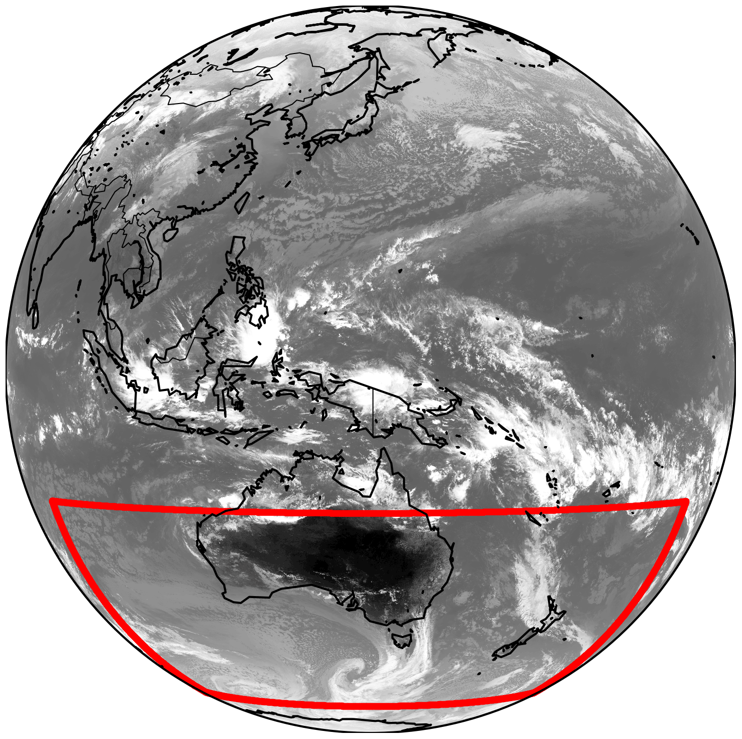
Figure 1A full disc image of Himawari-8 channel 11 on 15 February 2017 and the domain extent over the Southern Ocean outlined by the red line.
2.2 MCC cloud classification
Following McCoy et al. (2017), we focus on exploring the influence of the synoptic meteorology on open and closed MCC morphologies over the SO. The first step is to develop an algorithm to classify MCC clouds over the SO. As mentioned above, Wood and Hartmann (2006) first implemented an ANN for MCC morphology identification. More recently, several studies have applied a more advanced neural network model based on convolution tensor operations in a convolution neural network (CNN) for the identification and classification of MCC clouds (e.g. Rampal and Davies, 2020; Watson-Parris et al., 2021; Yuan et al., 2020). In deep learning, CNN models have been able to separate complex patterns into different categories. As Rampal and Davies (2020) pointed out, a deep-learning method based on spatial patterns is likely more advantageous because it can use a direct satellite channel for model training rather than an inferred product such as liquid water path (Wood and Hartmann, 2006).
For the classification, we settle on three categories. These are open MCC, closed MCC, and others. The category of others is used for other cloud types (e.g. mid- and high-level clouds, stratus, and disorganized MCC), ocean, and land. In contrast to other studies, we did not perform a separation into more cloud categories due to the limited capacity of hourly data processing. The brightness temperature from channel 11 (8.6 µm) is used as the main input for neural network model training, while the other Himawari-8 observations and products are used as filtering and contextual information for building up the manually labelled training data set. Figure 2 shows an example scene used to identify the three categories. For the category others, Fig. 2 shows a subscene consisting of stratus and nimbostratus, according to JAXA clouds product (not shown).
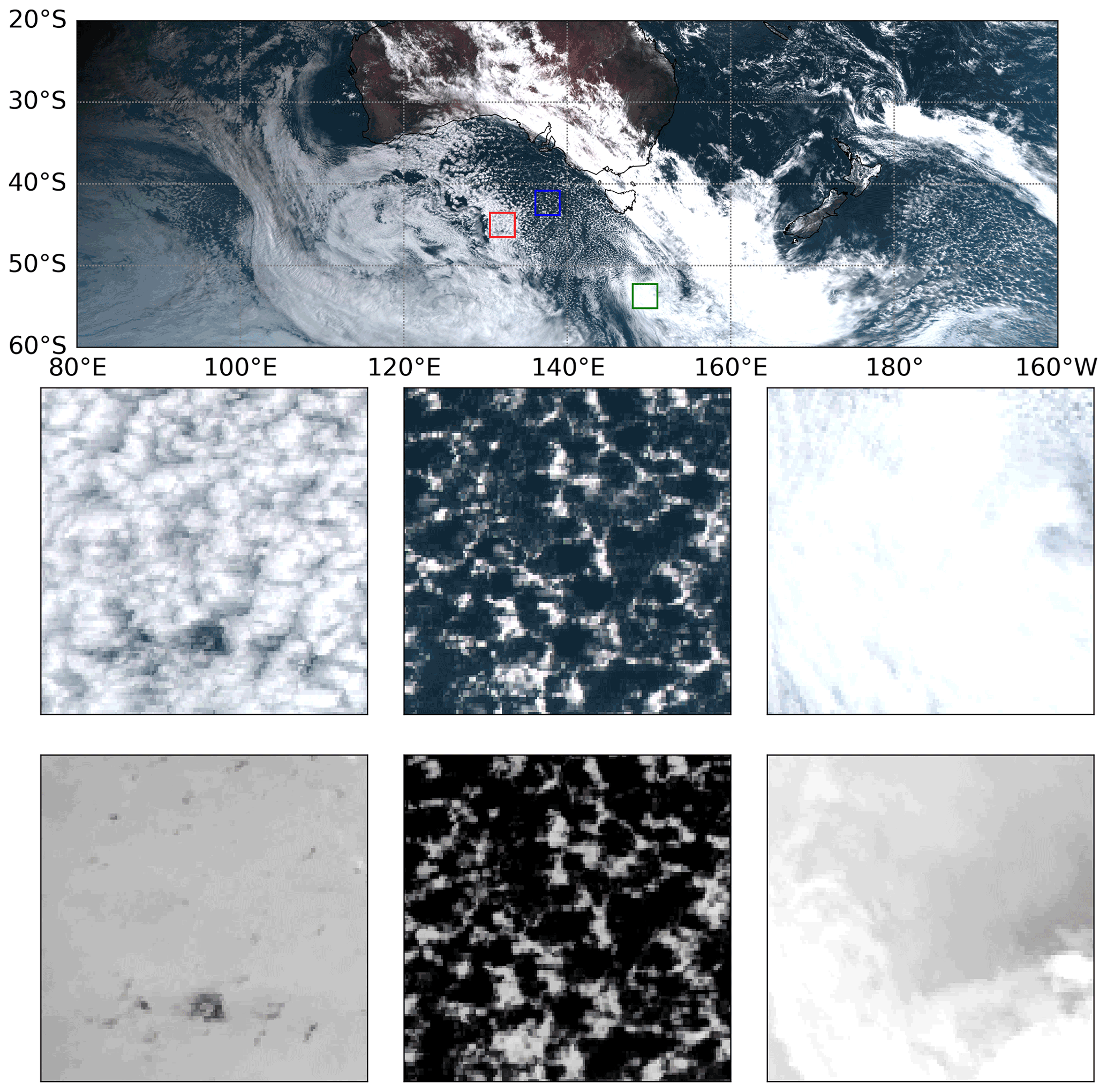
Figure 2An example scene of AHI Himawari-8 on 14 January 2016 at 00:00 UTC used as training. The full domain is shown in the top row, and the second and third rows show the visible and channel 11 views, respectively. The closed MCC structures (red square and first column), open MCC structures (blue square and second column), and others (green square and third column) are also shown.
2.2.1 CNN model structure
Our classification scheme of MABL clouds is based on a hybrid CNN model built using the TensorFlow Python package, which uses observations from the Himawari-8 geostationary satellite to classify the observed domain as open MCC, closed MCC, or others. The inputs to the CNN model consist of hourly data from 2016 to 2018 of brightness temperature from AHI Himawari-8 at 5 km resolution. At this resolution, the domain size is 801 × 2401 grid points. Different infrared channels and combinations of them were tested as inputs to the neural network, with channel 11 having the best performance. The hybrid nature of the model comes from having both scalar and spatial input layers, where the spatial input is a window of the brightness temperature, while the scalar inputs are the solar and satellite zenith and azimuth angles. The window of the brightness temperature is meant to provide enough morphological information about the cloud configuration, while the angles provide the model with information regarding distortions in the viewing and irradiation angle. Adding this information to the model showed improved accuracy. From the AHI domain, each grid point is classified by providing the hybrid model with a 2D array of the normalized brightness temperature (channel 11) centred at the point to be classified and the corresponding satellite and solar angles for that grid point. After a sensitivity analysis, a window of 16 × 16 points (∼ 80 km × 80 km) was used for the brightness temperature array, which provided the highest accuracy with the lowest computational cost. In effect, each grid point is classified using the information of that grid point, the 255 surrounding points, the satellite viewing angle, and the solar angle. The model structure is composed of three convolutional layers that process the spatial input (brightness temperature array), two layers that process the angles, and two layers applied after the output from the convolutional layers and the angle layers are concatenated. The output of the model is a three-element vector whose elements sum up to 1 and are interpreted as the probability of the tested point to correspond to one of the three classes. The point is assigned the category corresponding to the element with the highest probability.
2.2.2 Training data set
The model was trained in a supervised fashion, using a data set created by manually identifying areas where only open MCC, closed MCC, or neither were exclusively present in a similar methodological manner used in previous studies (Rampal and Davies, 2020; Watson-Parris et al., 2021; Wood and Hartmann, 2006; Yuan et al., 2020). In order to ensure that the labelling of the open and closed MCC was consistent, the structure of the MCC clouds must follow the conservative criterion that open MCC must be an open cell cloud, which looks stringy and forms a group of open rings, while the closed MCC must be a closed cell cloud, which looks`bubbly (Watson-Parris et al., 2021). Figure 2 shows a scene with examples for open and closed MCC. The transitions from open to closed MCC clouds were, by default, classified as other. Although, an infrared channel might entail less contrast compared to a visible channel, which is particularly important in the identification of closed MCCs, our sample selection criteria is very conservative and only uses samples where it is clearly possible to observe closed MCC clouds, as can be seen in the example in Fig. 2.
Based on these criteria, a training data set of approximately 400 independent scenes was built for each category, for the period between January 2016 and December 2018, and carefully chosen such that a relatively equal number of samples are taken from all seasons, allowing for a wide range of synoptic meteorology, solar zenith angles, and diurnal variation. All MCC areas selected are predominantly low-level clouds, defined as cloud-top height less than 3.5 km, while the areas representing the others class were selected from all other scenes, including areas with no clouds and land. These labelled areas accounted for ∼ 2.7×10⁶ individual pixels in total, where ∼ 1.2×10⁶ are under the open MCC category, ∼ 0.6×10⁶ are under the closed MCC category, and the remainder (∼ 0.9×10⁶) are under the others category. In total, 80 % of these data were used to train the model, while the other 20 % were used to validate it.
2.2.3 Training performance
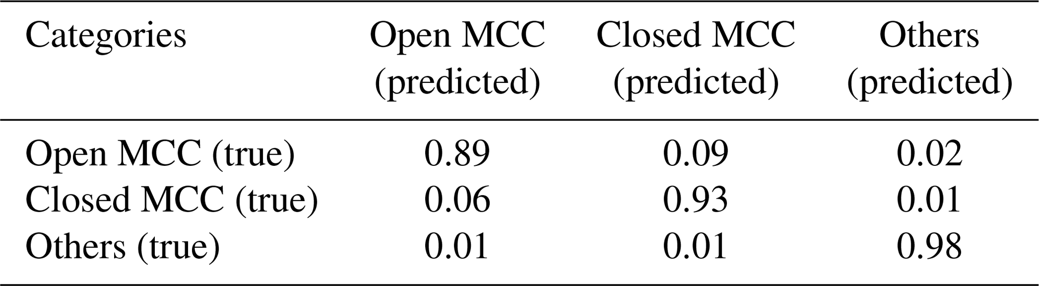
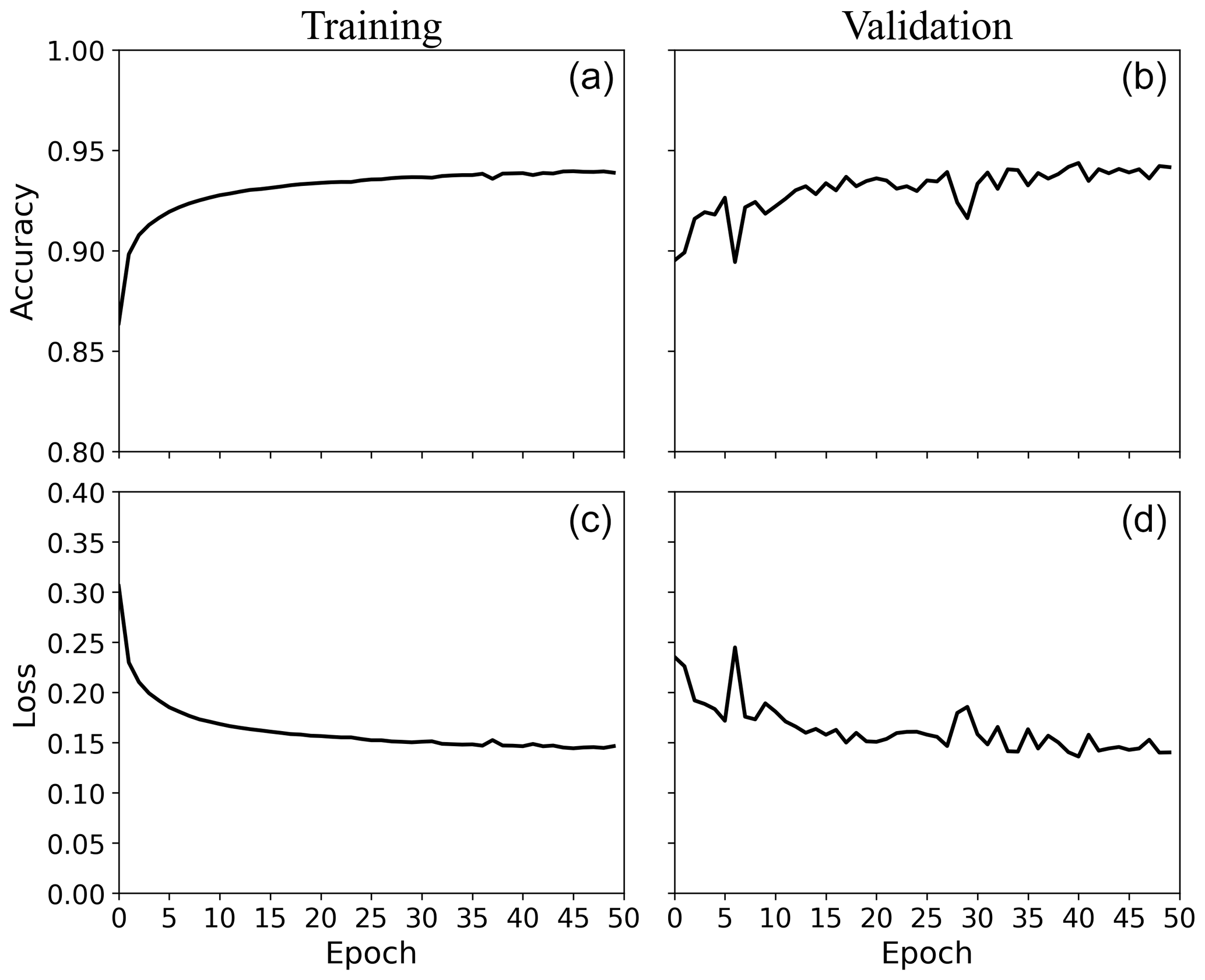
In terms of accuracy, the model's training reaches a plateau fairly quickly, i.e. within about 45 iterations through the whole data set (epochs), with maximum training and validation accuracies around 93.7 % and 4.1 %, respectively (Fig. 3). The confusion matrix of the validation data set is shown in Table 1. This matrix displays a summary of the prediction results averaged individually for each category. The trained model shows an average precision of about 89 % across the different types, with the open MCC category exhibiting the lowest accuracy, mainly due to having the lowest training sample size.
Table 1Confusion matrix of the model predictions on test data.
2.3 The SO meteorology and polar front
The SO meteorology is strongly influenced by the storm track, which is characterized by frequent and deep midlatitude cyclones that drive persistently strong zonal winds (Mace et al., 2009; Mace and Zhang, 2014). MABL clouds are commonly present in the cold sector of extra-tropical cyclones and in marine cold air outbreaks (Field et al., 2011; Kay et al., 2016; Naud et al., 2014; Williams et al., 2013). Figure 4a shows the frequency of 10 m winds exceeding 15 m s−1 from the European Centre for Medium-Range Weather Forecasts (ECMWF) ERA5 reanalysis across our domain (Hersbach et al., 2020), where midlatitudes and high latitudes are characterized by frequent high wind speeds. The cold sector located northwest of the cyclone centre is a region of large-scale subsidence dominated by MABL clouds, where the inversion strength and cloud fraction are related because the inversion controls the mixing at the cloud top (Klein and Hartmann, 1993). Over the post-cold-frontal SO regions, a strong inversion has been observed (more stable conditions), which is favourable for the generation of shallow convection (Lang et al., 2018). About 80 % of the marine cold air outbreaks occur in association with the passage of cyclones, and they are characterized by a large air–sea temperature difference, where the cold air masses impinge on warmer midlatitude air (Papritz et al., 2015). The warm water/cool air contrast increases the flux of energy and moisture from the surface into the boundary layer, which influences the development of MABL clouds (Abel et al., 2017; Fletcher et al., 2016a). The strength of the SO turbulent heat flux is strongly controlled by marine cold air outbreaks (Papritz et al., 2015). In the high latitudes and midlatitudes, a transition between closed MCC clouds and open MCC clouds occurs with the passage of cyclones and cold air outbreaks (McCoy et al., 2017).
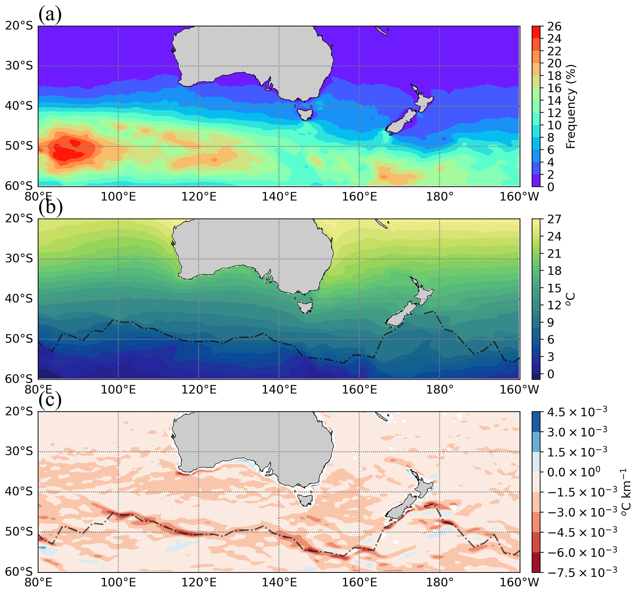
Figure 4(a) Frequency (%) of 10 m winds exceeding 15 m s−1 from ERA5, (b) mean SST from ERA5 reanalysis, and the corresponding (c) SST gradient. The period between 2016 and 2018 is shown. Black lines indicate the position of the polar front derived from ERA5 SST gradients.
Inatsu and Hoskins (2004) used global circulation models to demonstrate that the major determinant of the lower troposphere storm track intensity over the SO was the enhanced midlatitude sea surface temperature (SST) gradients or polar front (Dong et al., 2006; Moore et al., 1999). Dong et al. (2006) defined the polar front as the strong SST gradient, where a strong gradient is determined to be the southernmost location at which the SST gradient exceeds 1.5 × 10⁻² ∘C km−1. Figure 4b and c show the mean SST and the SST meridional gradient from ERA5 reanalysis products between 2016 and 2018. In our case, we define the polar front as the southernmost maximum in the SST gradient. The maximum SST gradient varies spatially in its mean position (Fig. 4c). The mean SST gradient path is further north in the Indian Ocean sector at ∼ 43∘ S and moves poleward until it reaches ∼ 57∘ S at 150∘ E. This north–south range of the mean SST gradient path is about 15∘. Although the definition of the polar front in Dong et al. (2006) differs from our estimates in Fig. 4b, the mean polar path is consistent with the SST gradients from ERA5 and within the variability that corresponds to different observations and reanalysis products, as shown in Dong et al. (2006).
2.3.1 Synoptic data
The relationships between MCC clouds and two synoptic features common to the SO storm track, namely cold fronts and extra-tropical cyclones, were explicitly studied. These features were calculated using ERA5. Extra-tropical cyclones were identified using the cyclone detecting and tracking algorithm developed by Pezza et al. (2008) and Murray and Simmonds (1991). This identification is based on the 3 h mean sea level pressure (MSLP). The algorithm transforms the MSLP latitude–longitude grid to a polar stereographic grid and then searches for the local maximum in the Laplacian of the MSLP field. Each cyclone identified is assigned as either open or closed, based on whether it has an open or closed isobar around the minimum. To select only meteorologically significant systems, the pressure minimum had to satisfy a strength criterion, where those between 0.2 and 0.7 hPa (∘ lat)−2 were classified as weak and those with the strength greater than 0.7 hPa (∘ lat)−2 were classified as strong (see Lim and Simmonds, 2007, for complete details). Here, we use the term cyclone to refer to a specific feature at a specific time, rather than a complete life cycle. Over our domain and for the study period, a total of 22 690 strong cyclone centres were identified.
The objective identification of cold fronts is based on the method developed by Hewson (1998) and improved by Berry et al. (2011). This algorithm identifies frontal points along the maximum of the horizontal gradient of the wet‐bulb potential temperature at 850 hPa. The diagnosed fronts are then categorized into cold, warm, and quasi‐stationary fronts, according to different speed ranges. The analysis by Berry et al. (2011) with the ECMWF ERA-Interim reanalysis found the highest front frequency in the midlatitude storm tracks over the SO.
2.3.2 MCC cloud composites
For each cyclone centre identified, we extracted the MCC classification for each grid point in a 3000 × 3000 km square centred on the cyclone core to construct the composite structure. This cyclone centre composite allowed us to define a frame of reference, where the cold air side of the cyclone is commonly located in the northwestern and southwestern quadrants (e.g. Bodas-Salcedo et al., 2014; Lang et al., 2018; Truong et al., 2020).
The distance from a given grid point to the nearest cold front is defined as the distance along a line between the two that is aligned along the wind vector at the grid point. Considering that MCC clouds are mostly located in the cold sector, cold fronts have to be eastward of the MCC systems within a distance of 20∘, where a MCC system is defined as a continuous group of grid points classified as either closed or open MCCs. We use the term system to refer to an event at a specific time rather than a complete life cycle. For the wind direction, we use ERA5 wind components at 850 hPa. The frequency of the open and closed MCC cloud is estimated by distance into 100 km bins to produce a composite across the cold sector. A total of 25 654 open MCC systems and 15 722 closed MCC systems were associated with a cold front between the 2016 and 2018 period, which is composed of approximately 26 280 satellite images.

Figure 5Example scenes of AHI Himawari-8 (brightness temperature; channel 11) and MCC structures identified by the CNN. (a, b) Summertime on 17 February 2018 at 02:00 UTC and (c, d) wintertime on 10 June 2016 at 21:00 UTC. The red squares delimit the magnified area in subscenes.
2.4 Examples of the classification
There are two examples of classified brightness temperature images under a post-frontal environment for the winter and summer seasons in the midlatitude shown in Fig. 5. The summertime scene (Fig. 5a) shows a cloud field of MCC clouds in the cold sector of an extra-tropical cyclone located at ∼ 59∘ S. The cloud field shown in this example is midway through a transition from a closed to an open MCC cloud, where closed MCC are moving from high latitudes advected over a warmer ocean. Similarly, Fig. 5c shows an example for wintertime, where a large high-pressure system is present over Australia, according to the mean sea level pressure from the Australian Bureau of Meteorology (not shown). Located in the southern edges, the MCC cloud field displays a transition from a closed to an open MCC cloud followed by frontal clouds. The classification results are overlain on two subscenes of the channel 11 brightness temperature image (Fig. 5b, d), where low-cloud-dominated areas show the presence of the two morphology types. The areas not classified correspond to others; for example, Fig. 5b shows a group of clouds to the south and southeast that are mostly altostratus clouds. For these two examples, one can visually confirm that the CNN performs reasonably well in selecting the open and closed MCC morphologies and their transitions.
The CNN model was run on all the hourly brightness temperature images over the domain in Fig. 1 between 2016 and 2018. For this period, 25 494 images were processed and classified into the categories of open MCC, closed MCC, and others.
3.1 MCC climatology
The geographical distribution of the annual relative frequency of occurrence of open and closed MCC clouds is illustrated in Fig. 6a and b, respectively. The frequency of occurrence of MCC clouds is defined as the number of times a cloud type (e.g. open MCC cloud) is observed in a grid point and time period divided by the total time. First, it is noted that the spatial distribution of MCC clouds features a ∼ 15∘ broad band across the domain. This band is located further south, compared to the southeastern Indian Ocean, which is perhaps due to the influence of the Australian and New Zealand land masses. This is consistent with the distribution of low-level clouds from CloudSat/CALIPSO data in Muhlbauer et al. (2014), which showed low-cloud fraction peaks south of Australia and lower frequencies towards high latitudes.
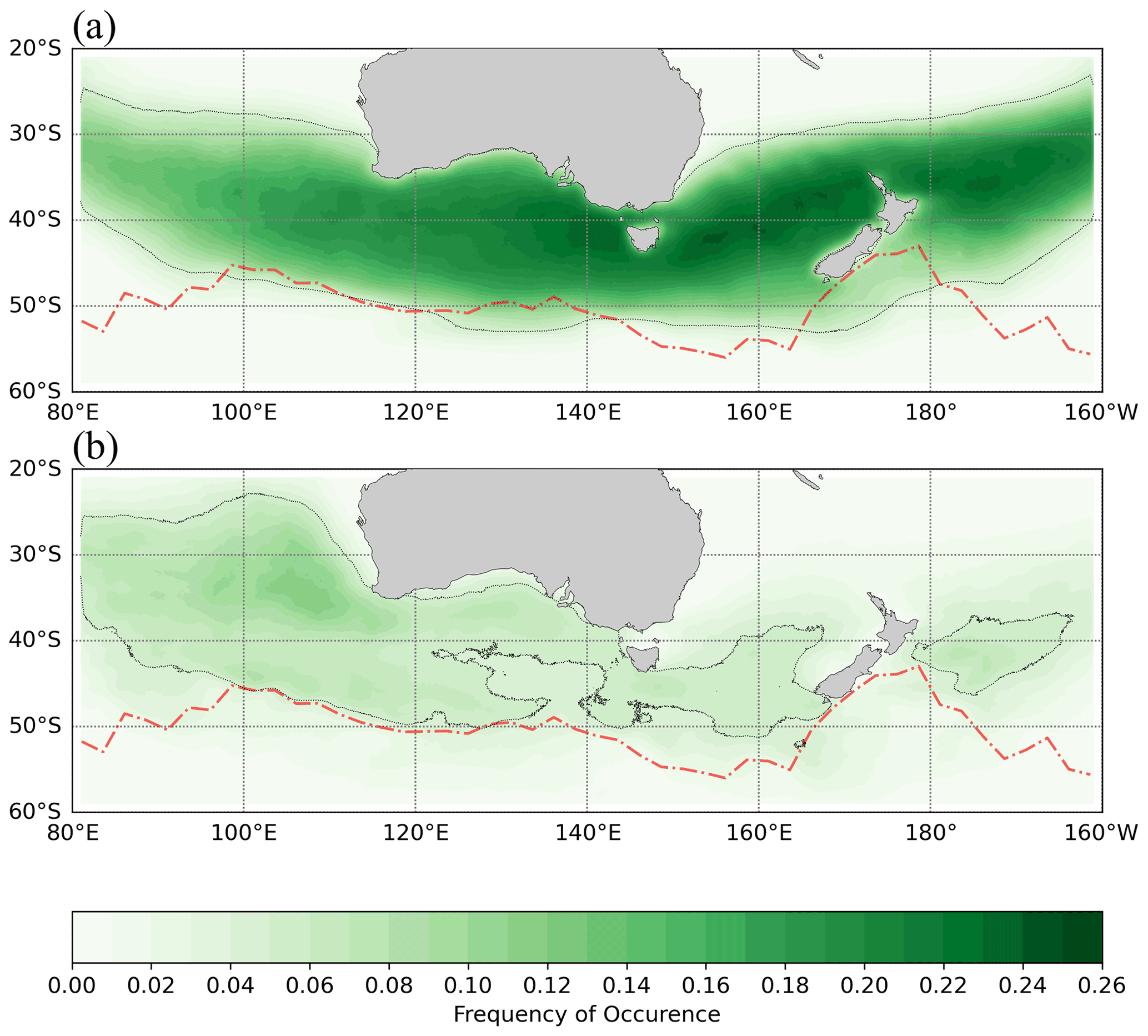
Figure 6Distribution of the frequency of occurrence of the MCC structures for the period 2016–2018. (a) Open MCC and (b) closed MCC structures. Red lines indicate the position of the polar front derived from ERA5 SST gradients. The dotted black lines show the contour level of 0.05 %.
Figure 6a shows that open MCC clouds exhibit a relatively uniform distribution across midlatitudes. They peak in the area of the storm track between 40 and 50∘ S and have two local maxima over the surrounding ocean west of Tasmania (23 %) and the Tasman Sea (25 %). The presence of open MCC over the storm track is likely associated with marine cold air outbreaks and frontal passages. While the closed MCC clouds are less frequent than the open MCC, they are most predominant (12 %) over the southeastern Indian Ocean (Fig. 6b) where persistent stratocumulus decks have been observed by previous studies (e.g. Atkinson and Zhang, 1996; Klein and Hartmann, 1993; Muhlbauer et al., 2014). This region is located in the large-scale subsidence region west of Australia, commonly influenced by strong high-pressure systems and the upwelling of cold oceanic waters (Atkinson and Zhang, 1996). As with open MCCs, closed MCC clouds are likely associated with marine cold air outbreaks in these regions. Overall, the contributions of closed MCC are considerably lower, with the frequency of occurrence ranging from about 5 % to 12 %. A shift from closed to open MCCs clouds is seen from the southeastern Indian Ocean into the SO immediately south of Australia, likely indicating that the stratocumulus clouds moving from the west break up into shallow cumulus clouds. Further poleward, the occurrence of both MCC types tends to decrease with a slightly higher presence of closed MCC.
A blocking effect of New Zealand is observed eastward of ∼ 170∘ E, as shown by a considerable decrease in the frequencies for both MCC types. Similarly, the area eastward of Tasmania presents lower frequencies due to a land effect from the island. A strong relationship between the MCC classifications and the SST gradients over the SO is seen in Figs. 4c and 6. The location of the southern boundaries for both classifications clearly shows an alignment with the maximum SST gradients over the domain. We also notice that low frequencies for closed MCC are associated with low SST gradients; for instance, a band between 40–50∘ S and 100–140∘ E shows a local minimum for both closed MCC occurrences and SST gradients. This relationship emphasizes the temperature contrast between the cold air moving from high latitudes above relatively warmer water, creating a dynamically favourable condition for MABL cloud development. At high latitudes, the occurrence of both morphologies tends to decrease with a slightly higher presence of closed MCC. We note that, at the high latitudes, poleward of the polar ocean front, mid-level clouds are commonly present (Mace et al., 2009; Truong et al., 2020), which obscures the observation of any boundary layer clouds from passive satellite instruments. This reduction in the MCC frequencies may also be related to the higher wind speeds at surface level, as shown in Fig. 4a. The highest wind speed frequencies of winds exceeding 20 m s−1 are at the western portion of our domain, from ∼ 80 to 100∘ E, and southward of New Zealand, from ∼ 160∘ E to 170∘ W. These two regions correlate well with a reduced fractional MCC cloud cover (Fig. 6). A local maximum is observed northeast of New Zealand; this region coincides with a local maximum of cold fronts associated with the South Pacific convergence zone (Berry et al., 2011). However, the MCC classification by Rampal and Davies (2020) primarily shows the occurrence of disorganized MCC in this area. We believe that our model is struggling to separate open from disorganized MCC over this area. This discrepancy also seems to be present in Fig. 5b, where clouds in the southeastern corner of the domain are classified as open MCCs. Uncertainties in the separation of disorganized and open MCC using a CNN was also reported by Yuan et al. (2020).
The seasonal cycle of the frequency of occurrence for MCC classifications is shown in Fig. 7. A considerable seasonal cycle is found for open MCC. The maximum frequency of occurrence of open MCC is found during the spring season (September–November; SON) over the Tasman Sea between 35 and 40∘ S (28 %). Similarly, west of Tasmania and the southern Pacific Ocean, between about 30 and 40∘ S, open MCC have higher frequencies above 25 % of the time. During summer (December–February; DJF), open MCC frequencies are lower, with a considerable reduction in the frequency of occurrence in sectors such as the southern Pacific Ocean and the southeastern Indian Ocean (∼ 15 % during summer). Similar to McCoy et al. (2017), open MCC frequency has the largest seasonal cycle; however, they found the maximum frequency for open MCC occurrence during winter. A shift of the maximum further poleward is also observed during the summer season, likely due to the influence of the Hadley cell extending further poleward (as does the storm track). The strong seasonality in the open MCC frequency might be linked to the lower frequency of occurrence of cold air outbreaks and the associated advection of cold air over warmer ocean surfaces, both reaching the minimum during summer months.

Figure 7Seasonal cycle of the frequency of occurrence of MCC structures for the period 2016–2018. Shown are open MCC (left) and closed MCC (right) structures. Seasonal means are shown for summer (DJF), autumn (MAM), winter (JJA), and spring (SON).
Compared to open MCC, the occurrence frequency of closed MCC shows less interseasonal variability. Closed MCC maxima are present over the southeastern Indian Ocean with a peak of 13 % during summer. For the region west of Tasmania, the Tasman Sea, and the southern Pacific Ocean, summer shows a narrower band of closed MCC frequencies compared to the other seasons. Similarly, to open MCC clouds, the frequency peak moves poleward during summer (along with the storm track).
3.1.1 Diurnal cycle
Figure 8 shows the diurnal cycle of the frequency of occurrence for the annual mean and is sorted by season for a latitudinal band between 40 and 50∘ S. Looking at the annual mean (Fig. 8a), the diurnal cycle of closed MCC exhibits a pronounced daily cycle with a distinct 24 h phasing. A maximum is found during night and/or early morning, with a peak of 14 % before sunrise at 04:00 local standard time (LST) and a minimum at 14:00 LST (9.9 %). At approximately sunset, the mean observed occurrence reaches its lowest point below 10 % and increases through the night until approximately sunrise, with a range of the cycle of ∼ 4 %. The standard deviation shows that the variability is approximately constant around 5 % throughout the day. While a diurnal cycle was identifiable in all seasons for closed MCC, it was most intense during the warmer months, the austral summer (December– February; DJF), and spring (SON), as would be expected. For the winter (JJA) and autumn (March–May; MAM) seasons, the diurnal cycle is relatively flat through much of the day. The standard deviation also shows a low and constant variability at approximately around 5 % throughout the day for all the seasons.
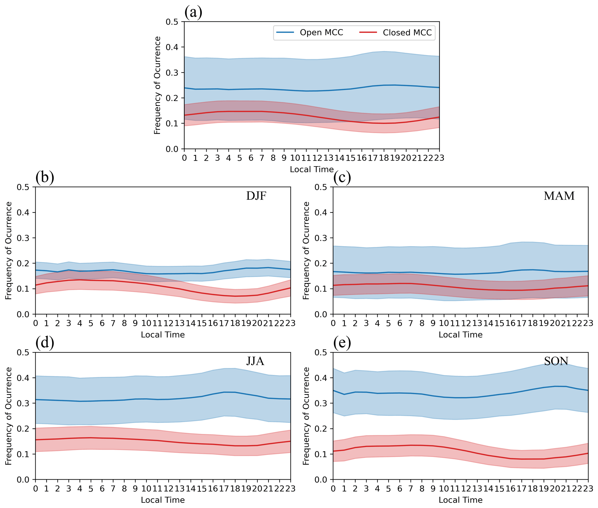
Figure 8Diurnal cycle of the frequency of occurrence of MCC structures for the period 2016–2018. Shown are open MCC (blue) and closed MCC (red) structures. Seasonal means are shown for summer (DJF), autumn (MAM), winter (JJA), and spring (SON). Shadings represent 1 standard deviation. Frequencies are calculated for the latitudinal band between 40 and 50∘.
In contrast, the diurnal cycle of open MCC is less distinct, with a maximum of 25 % in the afternoon at 18:00 LST. Compared to the closed MCC, the standard deviation for open MCC shows more variability throughout the day (∼ 10 %). The open MCC occurrence shows higher afternoon peaks for the austral winter and spring, with a frequency of occurrence higher than 30 % throughout the day, while summer and autumn are relatively flat through much of the day and at frequencies lower than 20 %. The seasonal standard deviation shows larger differences between summer and the other seasons, with a low variability during the summer season (∼ 2 %) and much higher for winter, spring, and autumn (∼ 10 %).
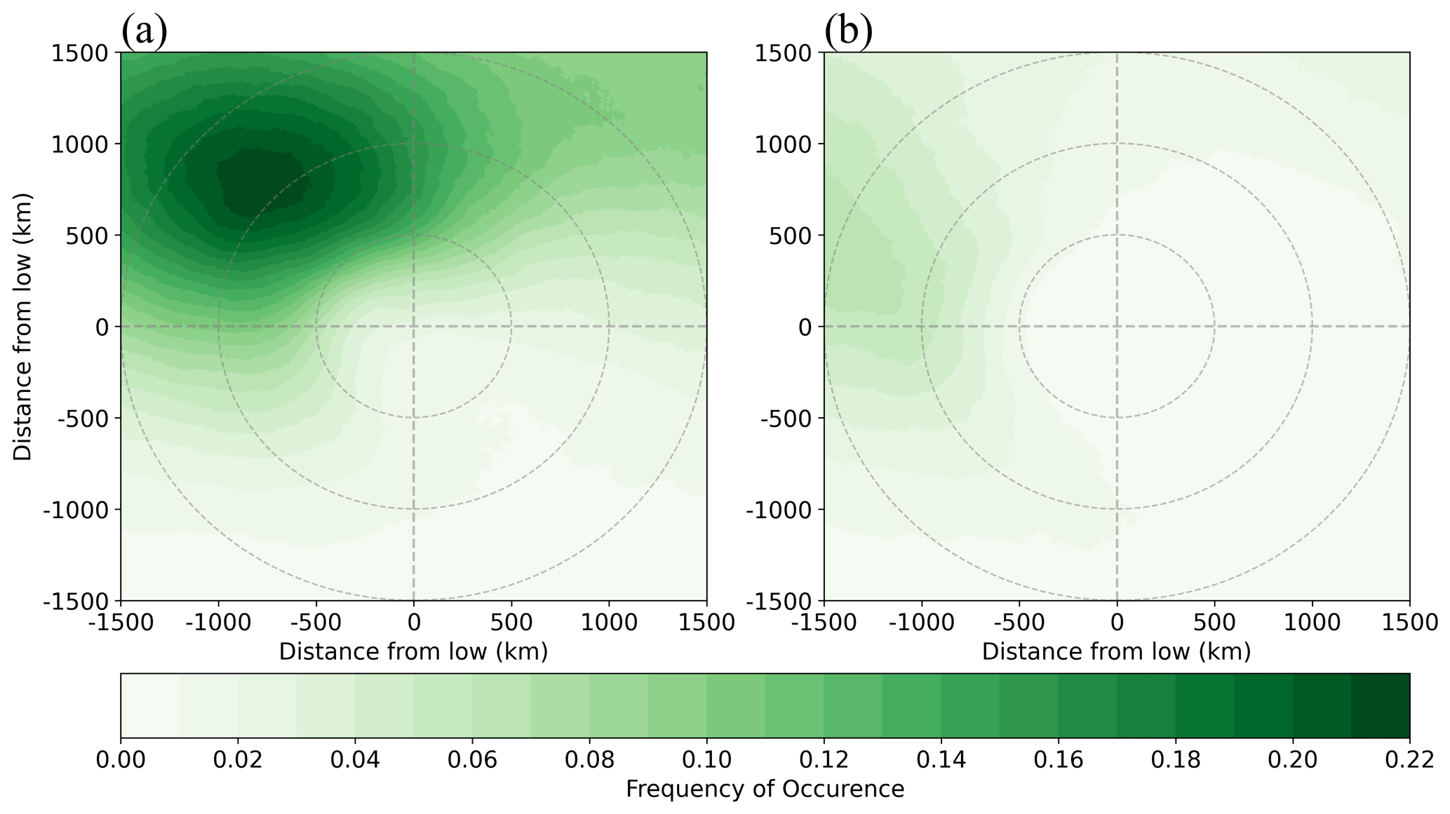
Figure 9Distribution of open and closed MCC structures in the context of the composite extra-tropical cyclones. Concentric circles indicate distances of 500, 1000, and 1500 km from the cyclone centre.
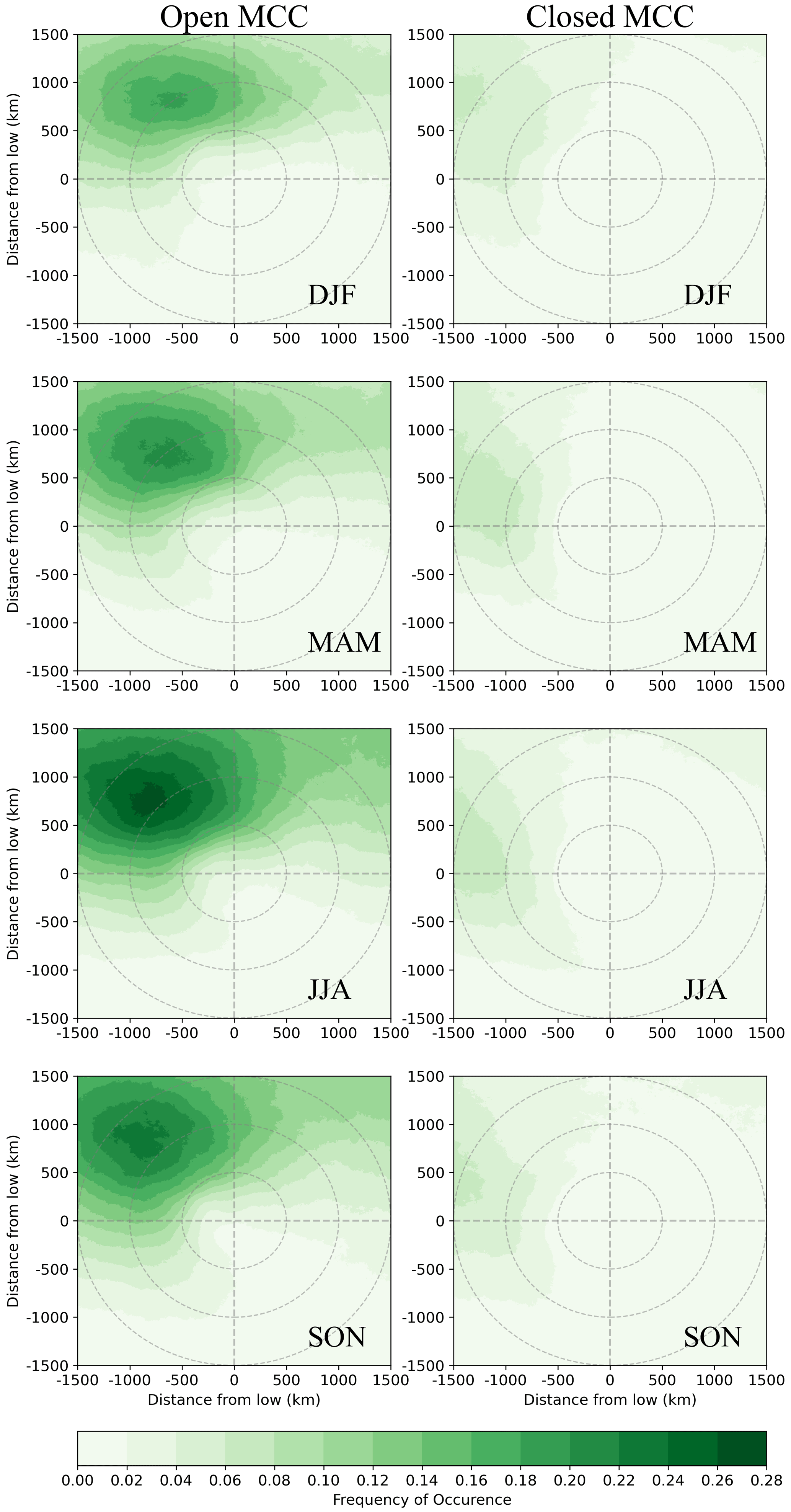
Figure 10Seasonal distribution of open and closed MCC structures in the context of the composite extra-tropical cyclones. Shown are open MCC (left) and closed MCC (right) types. Seasonal means are shown for summer (DJF), autumn (MAM), winter (JJA), and spring (SON). Concentric circles indicate distances of 500, 1000, and 1500 km from the cyclone centre.
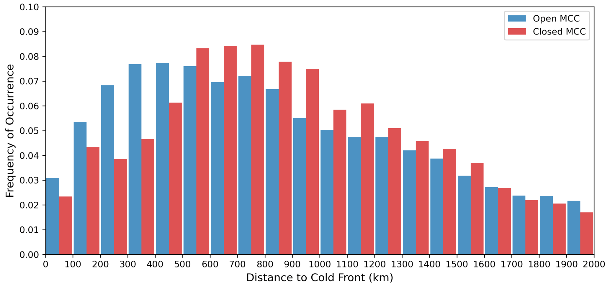
Figure 11Histogram of the relative frequencies of open and closed MCC in the post-cold-front sector. Graphs are sorted by distance with 100 km bins.
3.2 MCC relationship to extra-tropical cyclones and cold fronts
In this section, we investigate the main characteristics of the MCC clouds relative to the extra-tropical cyclones and cold fronts. The role of both cyclones and cold fronts is analysed to find a relationship between these synoptic conditions and MCC clouds that can explain the annual variability in the spatial pattern frequency and MCC cloudiness.
First, we look at the relationship between extra-tropical cyclones and MCC clouds using cyclone centre composites. The frequency of open MCC (Fig. 9a) has a maximum movement equatorward of a low pressure centre and westward of the cold frontal zone and lower frequencies poleward. This maximum reaches 22 % about ∼ 900 to 1300 km from the cyclone centre. This sector on the western side of the cyclone is, on average, a region of colder temperatures, lower moisture amounts, and lower precipitation than east of the low pressure centre (e.g. Bauer and Del Genio, 2006; Lang et al., 2018; Naud et al., 2014; Truong et al., 2020). A lower frequency of occurrence for open MCC is observed across the warm frontal zone, and open MCC extends into the warm sector on the eastward side of the low pressure centre, with frequencies between 2 % and 10 %. We examine the seasonal cycle to help determine the synoptic factors in open MCC cloud development (Fig. 10). The peak concentration of open MCC is found to be 27 % during the winter season, with the peak being at ∼ 1200 km from the cyclone core. The lowest frequencies are found during the summer season with a peak of 19 %. The distance of the peaks from the cyclone centre shows a small seasonal shift, moving further away, from 1000 km during the winter and spring seasons to closer distances between 800 and 1000 km during the summer and autumn seasons. This shift in the location of the peak is likely to be related to the larger extension and intensity of the wintertime extra-tropical cyclones (Simmonds and Keay, 2000), with more open MCC generated further away from the low centres.
The closed MCC cloud maximum tends to occur on the western side of the low centres and in the wraparound sector at the southwest of the open MCC but with a much lower frequencies that peak at 7 %. The peak frequency is located between ∼ 1300 and 1500 km from the cyclone core (Fig. 9b), which is further away than that of the open MCC. Winds over this area are primarily cold air from the southwest, indicating that closed MCC clouds move behind the open MCC clouds. According to Naud et al. (2014), the western side of the low centre is characterized by low-level clouds, where the average cloud-top height, using the Multi-angle Imaging SpectroRadiometer (MISR) observations, is found to be below 3 km. The frequency of the closed MCC type shows a much weaker interseasonal variability (Fig. 10) compared to that of the open MCC. Slightly higher frequencies are found during the winter season, with a peak of 8.1 %, while the minimum peak is observed during the summer season (6.7 %). Note that it is likely that the occurrence of closed MCC is higher outside of the 1500 × 1500 km window of the figures. The timing and location of the open MCC cloud seasonality around the cyclone centres is consistent with the connection to marine cold air outbreaks. Over the high latitudes and midlatitudes, the marine cold air outbreak frequencies peak in hemisphere winters (Fletcher et al., 2016b).
To explore the distribution of the MCC morphologies under a post-cold-frontal environment, we focus our analysis in the cold sector, using the distance from cold fronts as a reference. We only consider MCC systems that are located west of the cold front; in total, 25 654 open MCC systems and 15 722 closed MCC systems were associated with a cold front. Figure 11 shows the frequency of occurrence sorted by distance into 100 km bins for open and closed MCC. The histogram for open MCC shows the highest frequencies within 300 to 600 km from the cold front line, reaching a maximum between 400 and 500 km (7.7 %). Beyond a 700 km distance, the frequency of open MCC decreases with distance from the cold front. The maximum for the closed MCC histogram is located approximately at a distance between 500 and 800 km, with a peak of 8.5 % between 700 and 800 km. The results show a clear difference in the location of the maximum for each MCC type. This difference in the location of the maximum is consistent with cyclone centre composites and the examples in Fig. 3, where open MCC clouds are moving ahead of the closed MCC, along with the mean flow, which is consistent with McCoy et al. (2017). For both morphologies, the histograms show low frequencies immediately behind the frontal line. A clear band behind the cold fronts was first observed during the Aerosol Characterization Experiment 1 (ACE-1) campaign in the 1990s (Bates et al., 1998; Suhre et al., 1998). More recently, Lang et al. (2021) described the same clear band during the Clouds Aerosols Precipitation Radiation and atmospheric Composition over the Southern Ocean (CAPRICORN) I research voyage. Significant changes in the distribution of open and closed MCC between the seasons are not observed (not shown).
High-frequency geostationary satellite observations over the Southern Ocean (SO) are used to explore how marine atmospheric boundary layer (MABL) clouds are organized in mesoscale cellular convection (MCC) morphologies. We first focus on developing a convolution neural network (CNN) model to identify and classify open and closed MCC clouds based on 3 years of Himawari-8 satellite data from 2016 to 2018 and then to study their relationship to synoptic systems over the SO. The climatology showed that open MCC clouds are roughly uniformly distributed over the storm track across midlatitudes and have local maxima over the surrounding ocean west of Tasmania and New Zealand, 23 % and 25 % of the time, respectively, while closed MCC clouds are most predominant in the southeastern Indian Ocean (12 % of the time), which is an area characterized by persistent stratocumulus decks (Klein and Hartmann, 1993). Our results find that closed MCC clouds are less prevalent at high latitudes than found in previous studies using MODIS (McCoy et al., 2017; Muhlbauer et al., 2014). The algorithm used in Muhlbauer et al. (2014) and McCoy et al. (2017), however, is limited in that it only used liquid water path retrievals to classify the MCC cloud type (Wood and Hartmann, 2006). Over mid- and high-latitude oceans, the common presence of ice particles in clouds (e.g. Huang et al., 2017) and precipitation poses a significant challenge to this method. More recent studies have used CNN models to also show a weak presence of closed MCC at high latitudes (e.g. Mohrmann et al., 2021; Rampal and Davies, 2020). For example, Rampal and Davies (2020) found that closed MCC has a considerably lower frequency of occurrence (below 5 %) at high latitudes, while stratus clouds are the dominant MABL cloud type, with frequencies of occurrence ranging from about 20 % to 35 %. These differences from the work of McCoy et al. (2017) and Muhlbauer et al. (2014) can be attributed to a number of factors, such as differences in instrumentation, spatial resolution, and sampling periods. Nonetheless, our classification had the advantages that we used a more advanced neural network technique with samples located exclusively over our domain and from the fields of brightness temperature, which are less prone to retrieval errors at high solar zenith angles.
The climatological frequency of occurrence of open and closed MCC clouds showed a strong relationship to the sea surface temperature (SST) gradients. In regions of enhanced surface forcing due to the warmer ocean/colder air temperature contrast, the SST has been established as a driver mechanism for open MCC cloud development (McCoy et al., 2017). The maximum gradients of SST from ERA5 are aligned to the location of the southern boundaries, longitudinally, for both MCC types. When cold air from Antarctica moves equatorward over the polar front (i.e. marine cold air outbreaks), the strong SST gradient increases the flux of energy and moisture from the surface into the boundary layer and facilitates the development of MABL clouds (Abel et al., 2017; Brümmer, 1996; Fletcher et al., 2016b). McCoy et al. (2017) point out that these stronger fluxes denote a transition between closed MCC clouds from high latitudes to open MCC clouds. However, as mentioned above, our results showed lower frequencies at high latitudes, consistent with Rampal and Davies (2020) and Yuan et al. (2020). The lower frequencies of MCC morphologies at high latitudes are also consistent with the common presence of multilayer cloud structures within and above the MABL (Mace et al., 2009; Truong et al., 2020), which represents a challenge for the identification of MCC clouds using only cloud-top observations. In addition, we noted that MCC cloud cover in this region might be influenced by the frequent high wind speeds. The frequency of winds exceeding 25 m s−1, using ERA5, showed that the highest wind speed frequencies are in the western portion of our domain, from ∼ 80 to 100∘ E, and southward of New Zealand, from ∼ 160∘ E to 170∘ W. These two regions correlate well with a reduced fractional MCC cloud cover (Fig. 7). An open question related to this is whether frequent and strong winds disrupt the formation (or maintenance) of ideal open and closed MCC clouds, which is worthy of future research and explanation.
The hourly classification from AHI Himawari-8 channel 11 brightness temperature allowed the study of the diurnal cycle of both MCC morphologies (Fig. 8). The diurnal cycle of MABL clouds has been documented for decades, where a strong diurnal cycle has been identified (e.g. Nicholls, 1984; Minnis and Harrison, 1984). Our results showed that the frequency of occurrence of closed MCC exhibits a pronounced daily cycle, with a maximum during the night and/or early morning. On the other hand, the diurnal cycle of open MCC is almost absent. The difference between the two morphologies might occur because open MCC clouds are particularly influenced by large-scale surface forcing, while closed MCC clouds are more affected by longwave cloud-top cooling outside the subtropics (Kazil et al., 2014; Wood, 2012). In this sense, the diurnal cycle of closed MCC clouds is strongly influence by the incoming solar radiation. At night, in the absence of solar forcing, the MABL can become well mixed, and the cloud deck commonly thickens with the renewed access to moisture from the ocean surface (e.g. Lang et al., 2020; Nicholls, 1984; Minnis and Harrison, 1984). This diurnal cycle and its seasonality are consistent with a diurnal cycle of precipitation observed over the oceans between 35 and 50∘ S (e.g. Dai, 2001; Dai et al., 2007) and at Macquarie Island Station (54.62∘S, 158.85∘E; Lang et al., 2018), where precipitation is significantly more frequent at night and during summer. Previous studies suggest that precipitation arising from MABL is probably making a greater contribution than previously thought (Lang et al., 2018, 2020), so understanding its daily cycle is fundamental to understanding the source of uncertainties in the water budget over the SO (Behrangi et al., 2012, 2014).
An investigation of the distribution of MCC clouds around cyclones and cold fronts showed that, in the cold sector of extra-tropical cyclones, closed MCCs move along with the mean flow following open MCC clouds. This is consistent with the results found in McCoy et al. (2017) for composites of open and closed MCC around marine cold air outbreaks in the Southern Hemisphere. They found that, for the cloud evolution along sea level pressure contours, the closed MCC has the highest frequency at the start of the flow, while open MCC clouds are most frequent to the east.
It appears that the relationship between MCC clouds and SST gradients is stronger than previously reported. While McCoy et al. (2017) show that the relationship of the extreme temperature contrast between the cold polar air and warmer water favours the development of MABL, our results show that the gradients themselves delimit the distribution of open and closed MCC over the SO. This suggests that the closed MCC cloud is possibly more influenced by surface forcing over this region than previously thought.
The current methodology works well overall, yet the distribution over the northeastern sector of New Zealand presents uncertainties in the classification. With a further increase in training samples in the future over this region, and the inclusion of more categories such as disorganized MCC, it is expected that our CNN model can be further improved. Future work using this CNN model will focus on the role of large-scale environmental conditions. In particular, we are interested in studying how the spatial organization of MCC clouds contributes to the daily cycle of shallow cumulus clouds and precipitation.
All Himawari-8 data can be accessed using the following public website: https://www.eorc.jaxa.jp/ptree/index.html (Japan Meteorological Agency, 2021).
FL prepared the paper and performed most of the data analysis. FL and LA implemented the method to train the network model. FL prepared the training data. LA compiled the training data set. All co-authors provided editorial feedback on the paper.
The contact author has declared that neither they nor their co-authors have any competing interests.
Publisher’s note: Copernicus Publications remains neutral with regard to jurisdictional claims in published maps and institutional affiliations.
We thank Daniel Robbins, for his help with the artificial neural network.
This research has been supported by the Australian Research Council Discovery Projects (grant no. DP190101362).
This paper was edited by Zhanqing Li and reviewed by Robert Wood and two anonymous referees.
Abel, S. J., Boutle, I. A., Waite, K., Fox, S., Brown, P. R., Cotton, R., Lloyd, G., Choularton, T. W., and Bower, K. N.: The role of precipitation in controlling the transition from stratocumulus to cumulus clouds in a Northern Hemisphere cold-air outbreak, J. Atmos. Sci., 74, 2293–2314, https://doi.org/10.1175/JAS-D-16-0362.1, 2017. a, b
Ahn, E., Huang, Y., Chubb, T. H., Baumgardner, D., Isaac, P., de Hoog, M., Siems, S. T., and Manton, M. J.: In situ observations of wintertime low-altitude clouds over the Southern Ocean, Q. J. Roy. Meteorol. Soc., 143, 1381–1394, https://doi.org/10.1002/qj.3011, 2017. a, b, c
Atkinson, B. W. and Zhang, J. W.: Mesoscale shallow convection in the atmosphere, Rev. Geophys., 34, 403–431, https://doi.org/10.1029/96RG02623, 1996. a, b, c
Bauer, M. and Del Genio, A. D.: Composite analysis of winter cyclones in a GCM: Influence on climatological humidity, J. Clim., 19, 1652–1672, https://doi.org/10.1175/JCLI3690.1, 2006. a
Bates, T. S., Huebert, B. J., Gras, J. L., Griffiths, F. B., and Durkee, P. A.: International Global Atmospheric Chemistry (IGAC) project's first aerosol characterization experiment (ACE 1): Overview, J. Geophys. Res.-Atmos., 103, 16297–16318, https://doi.org/10.1029/97JD03741, 1998. a
Behrangi, A., Lebsock, M., Wong, S., and Lambrigtsen, B.: On the quantification of oceanic rainfall using spaceborne sensors, J. Geophys. Res.-Atmos., 117, D20105, https://doi.org/10.1029/2012JD017979, 2012. a
Behrangi, A., Stephens, G., Adler, R. F., Huffman, G. J., Lambrigtsen, B., and Lebsock, M.: An update on the oceanic precipitation rate and its zonal distribution in light of advanced observations from space, J. Clim., 27, 3957–3965, https://doi.org/10.1175/JCLI-D-13-00679.1, 2014. a
Berry, G., Reeder, M. J., and Jakob, C.: A global climatology of atmospheric fronts, Geophys. Res. Lett., 38, L04809, https://doi.org/10.1029/2010GL046451, 2011. a, b, c
Bessho, K., Date, K., Hayashi, M., Ikeda, A., Imai, T., Inoue, H., Kumagai, Y., Miyakawa, T., Murata, H., Ohno, T., Okuyama, A., Oyama, R., Sasaki, Y., Shimazu, Y., Shimoji, K., Sumida, Y., Suzuki, M., Taniguchi, H., Tsuchiyama, H., Uesawa, D., Yokota, H., and Yoshida, R.: An introduction to Himawari-8/9 – Japan's new-generation geostationary meteorological satellites, J. Meteorol. Soc. Japn.. Ser. II, 94, 151–183, https://doi.org/10.2151/jmsj.2016-009, 2016. a
Bodas-Salcedo, A., Williams, K., Field, P., and Lock, A.: The surface downwelling solar radiation surplus over the Southern Ocean in the Met Office model: The role of midlatitude cyclone clouds, J. Clim., 25, 7467–7486, https://doi.org/10.1175/JCLI-D-11-00702.1, 2012. a, b
Bodas-Salcedo, A., Williams, K. D., Ringer, M. A., Beau, I., Cole, J. N., Dufresne, J.-L., Koshiro, T., Stevens, B., Wang, Z., and Yokohata, T.: Origins of the solar radiation biases over the Southern Ocean in CFMIP2 models, J. Clim., 27, 41–56, https://doi.org/10.1175/JCLI-D-13-00169.1, 2014. a
Bodas-Salcedo, A., Hill, P., Furtado, K., Williams, K., Field, P., Manners, J., Hyder, P., and Kato, S.: Large contribution of supercooled liquid clouds to the solar radiation budget of the Southern Ocean, J. Clim., 29, 4213–4228, https://doi.org/10.1175/JCLI-D-15-0564.1, 2016. a, b
Brümmer, B.: Boundary-layer modification in wintertime cold-air outbreaks from the Arctic sea ice, Bound.-Lay. Meteorol., 80, 109–125, https://doi.org/10.1007/BF00119014, 1996. a
Dai, A.: Global precipitation and thunderstorm frequencies. Part II: Diurnal variations, J. Clim., 14, 1112–1128, 2001. a
Dai, A., Lin, X., and Hsu, K.-L.: The frequency, intensity, and diurnal cycle of precipitation in surface and satellite observations over low-and mid-latitudes, Clim. Dynam., 29, 727–744, https://doi.org/10.1007/s00382-007-0260-y, 2007. a
Diner, D. J., Asner, G. P., Davies, R., Knyazikhin, Y., Muller, J.-P., Nolin, A. W., Pinty, B., Schaaf, C. B., and Stroeve, J.: New directions in earth observing: Scientific applications of multiangle remote sensing, Bull. Am. Meteorol. Soc., 80, 2209–2228, https://doi.org/10.1175/1520-0477(1999)080<2209:NDIEOS>2.0.CO;2, 1999. a
Dong, S., Sprintall, J., and Gille, S. T.: Location of the Antarctic polar front from AMSR-E satellite sea surface temperature measurements, J. Phys. Oceanogr., 36, 2075–2089, https://doi.org/10.1175/JPO2973.1, 2006. a, b, c, d
Field, P., Bodas-Salcedo, A., and Brooks, M.: Using model analysis and satellite data to assess cloud and precipitation in midlatitude cyclones, Q. J. Roy. Meteorol. Soc., 137, 1501–1515, https://doi.org/10.1002/qj.858, 2011. a
Field, P. R., Cotton, R. J., Mcbeath, K., Lock, A. P., Webster, S., and Allan, R. P.: Improving a convection-permitting model simulation of a cold air outbreak, Q. J. Roy. Meteorol. Soc., 140, 124–138, https://doi.org/10.1002/qj.2116, 2014. a
Fletcher, J., Mason, S., and Jakob, C.: The climatology, meteorology, and boundary layer structure of marine cold air outbreaks in both hemispheres, J. Clim., 29, 1999–2014, https://doi.org/10.1175/JCLI-D-15-0268.1, 2016a. a
Fletcher, J. K., Mason, S., and Jakob, C.: A climatology of clouds in marine cold air outbreaks in both hemispheres, J. Clim., 29, 6677–6692, https://doi.org/10.1175/JCLI-D-15-0783.1, 2016b. a, b, c
Hartmann, D. L. and Short, D. A.: On the use of earth radiation budget statistics for studies of clouds and climate, J. Atmos. Sci., 37, 1233–1250, https://doi.org/10.1175/1520-0469(1980)037<1233:OTUOER>2.0.CO;2, 1980. a
Haynes, J. M., Jakob, C., Rossow, W. B., Tselioudis, G., and Brown, J.: Major characteristics of Southern Ocean cloud regimes and their effects on the energy budget, J. Clim., 24, 5061–5080, https://doi.org/10.1175/2011JCLI4052.1, 2011. a
Hersbach, H., Bell, B., Berrisford, P., et al.: The ERA5 global reanalysis, Q. J. Roy. Meteorol. Soc., 146, 1999–2049, https://doi.org/10.1002/qj.3803, 2020. a
Hewson, T. D.: Objective fronts, Meteorol. Appl., 5, 37–65, https://doi.org/10.1017/S1350482798000553, 1998. a
Hoskins, B. J. and Hodges, K. I.: A new perspective on Southern Hemisphere storm tracks, J. Clim., 18, 4108–4129, https://doi.org/10.1175/JCLI3570.1, 2005. a
Huang, Y., Chubb, T., Baumgardner, D., deHoog, M., Siems, S. T., and Manton, M. J.: Evidence for secondary ice production in Southern Ocean open cellular convection, Q. J. Roy. Meteorol. Soc., 143, 1685–1703, https://doi.org/10.1002/qj.3041, 2017. a, b
Inatsu, M. and Hoskins, B. J.: The zonal asymmetry of the Southern Hemisphere winter storm track, J. Clim., 17, 4882–4892, https://doi.org/10.1175/JCLI-3232.1, 2004. a
Japan Meteorological Agency (JMA): Himawari L1 Gridded data, EORC [data set], https://www.eorc.jaxa.jp/ptree/index.html, last access: 25 January 2021. a
Kay, J. E., Wall, C., Yettella, V., Medeiros, B., Hannay, C., Caldwell, P., and Bitz, C.: Global climate impacts of fixing the Southern Ocean shortwave radiation bias in the Community Earth System Model (CESM), J. Clim., 29, 4617–4636, https://doi.org/10.1175/JCLI-D-15-0358.1, 2016. a, b
Kazil, J., Feingold, G., Wang, H., and Yamaguchi, T.: On the interaction between marine boundary layer cellular cloudiness and surface heat fluxes, Atmos. Chem. Phys., 14, 61–79, https://doi.org/10.5194/acp-14-61-2014, 2014. a
Klein, S. A. and Hartmann, D. L.: The seasonal cycle of low stratiform clouds, J. Clim., 6, 1587–1606, https://doi.org/10.1175/1520-0442(1993)006<1587:TSCOLS>2.0.CO;2, 1993. a, b, c
Lang, F., Huang, Y., Siems, S., and Manton, M.: Characteristics of the Marine Atmospheric Boundary Layer Over the Southern Ocean in Response to the Synoptic Forcing, J. Geophys. Res.-Atmos., 123, 7799–7820, https://doi.org/10.1029/2018JD028700, 2018. a, b, c, d, e
Lang, F., Huang, Y., Siems, S. T., and Manton, M. J.: Evidence of a Diurnal Cycle in Precipitation over the Southern Ocean as Observed at Macquarie Island, Atmosphere, 11, 181, https://doi.org/10.3390/atmos11020181, 2020. a, b, c
Lang, F., Huang, Y., Protat, A., Truong, S., Siems, S., and Manton, M.: Shallow Convection and Precipitation Over the Southern Ocean: A Case Study During the CAPRICORN 2016 Field Campaign, J. Geophys. Res.-Atmos., 126, e2020JD034088, https://doi.org/10.1029/2020JD034088, 2021. a, b, c
Lim, E.-P. and Simmonds, I.: Southern Hemisphere winter extratropical cyclone characteristics and vertical organization observed with the ERA-40 data in 1979–2001, J. Clim., 20, 2675–2690, https://doi.org/10.1175/JCLI4135.1, 2007. a
Mace, G. G. and Zhang, Q.: The CloudSat radar-lidar geometrical profile product (RL-GeoProf): Updates, improvements, and selected results, J. Geophys. Res.-Atmos., 119, 9441–9462, https://doi.org/10.1002/2013JD021374, 2014. a
Mace, G. G., Zhang, Q., Vaughan, M., Marchand, R., Stephens, G., Trepte, C., and Winker, D.: A description of hydrometeor layer occurrence statistics derived from the first year of merged Cloudsat and CALIPSO data, J. Geophys. Res.-Atmos., 114, D00A26, https://doi.org/10.1029/2007JD009755, 2009. a, b, c
McCoy, I. L., Wood, R., and Fletcher, J. K.: Identifying Meteorological Controls on Open and Closed Mesoscale Cellular Convection Associated with Marine Cold Air Outbreaks, J. Geophys. Res.-Atmos., 122, 11678–11702, https://doi.org/10.1002/2017JD027031, 2017. a, b, c, d, e, f, g, h, i, j, k, l, m, n, o, p
McFarquhar, G. M., Bretherton, C. S., Marchand, R., et al.: Observations of clouds, aerosols, precipitation, and surface radiation over the southern ocean: An overview of CAPRICORN, MARCUS, MICRE, and SOCRATES, Bull. Am. Meteorol. Soc., 102, E894–E928, https://doi.org/10.1175/BAMS-D-20-0132.1, 2021. a
Minnis, P. and Harrison, E. F.: Diurnal variability of regional cloud and clear-sky radiative parameters derived from GOES data, Part I: Analysis method, J. Appl. Meteorol., 23, 993–1011, 1984. a, b, c, d
Mohrmann, J., Wood, R., Yuan, T., Song, H., Eastman, R., and Oreopoulos, L.: Identifying meteorological influences on marine low-cloud mesoscale morphology using satellite classifications, Atmos. Chem. Phys., 21, 9629–9642, https://doi.org/10.5194/acp-21-9629-2021, 2021. a
Moore, J. K., Abbott, M. R., and Richman, J. G.: Location and dynamics of the Antarctic Polar Front from satellite sea surface temperature data, J. Geophys. Res.-Ocean., 104, 3059–3073, https://doi.org/10.1029/1998JC900032, 1999. a
Muhlbauer, A., McCoy, I. L., and Wood, R.: Climatology of stratocumulus cloud morphologies: microphysical properties and radiative effects, Atmos. Chem. Phys., 14, 6695–6716, https://doi.org/10.5194/acp-14-6695-2014, 2014. a, b, c, d, e, f, g, h, i
Murray, R. J. and Simmonds, I.: A numerical scheme for tracking cyclone centres from digital data, Part I: Development and operation of the scheme, Austr. Meteorol. Mag., 39, 155–166, 1991. a
Naud, C. M., Booth, J. F., and Del Genio, A. D.: Evaluation of ERA-Interim and MERRA cloudiness in the Southern Ocean, J. Clim., 27, 2109–2124, https://doi.org/10.1175/JCLI-D-13-00432.1, 2014. a, b, c, d
Nicholls, S.: The dynamics of stratocumulus: Aircraft observations and comparisons with a mixed layer model, Q. J. Roy. Meteorol. Soc., 110, 783–820, https://doi.org/10.1002/qj.49711046603, 1984. a, b, c, d, e
Papritz, L., Pfahl, S., Sodemann, H., and Wernli, H.: A climatology of cold air outbreaks and their impact on air–sea heat fluxes in the high-latitude South Pacific, J. Clim., 28, 342–364, https://doi.org/10.1175/JCLI-D-14-00482.1, 2015. a, b
Pezza, A. B., Durrant, T., Simmonds, I., and Smith, I.: Southern Hemisphere synoptic behavior in extreme phases of SAM, ENSO, sea ice extent, and southern Australia rainfall, J. Clim., 21, 5566–5584, https://doi.org/10.1175/2008JCLI2128.1, 2008. a
Platnick, S., King, M. D., Ackerman, S. A., Menzel, W. P., Baum, B. A., Riédi, J. C., and Frey, R. A.: The MODIS cloud products: Algorithms and examples from Terra, IEEE T. Geosci. Remote Sens., 41, 459–473, https://doi.org/10.1109/TGRS.2002.808301, 2003. a
Rampal, N. and Davies, R.: On the Factors That Determine Boundary Layer Albedo, J. Geophys. Res.-Atmos., 125, e2019JD032244, https://doi.org/10.1029/2019JD032244, 2020. a, b, c, d, e, f, g, h
Rozendaal, M. A., Leovy, C. B., and Klein, S. A.: An observational study of diurnal variations of marine stratiform cloud, J. Clim., 8, 1795–1809, https://doi.org/10.1175/1520-0442(1995)008<1795:AOSODV>2.0.CO;2, 1995. a
Simmonds, I. and Keay, K.: Mean Southern Hemisphere extratropical cyclone behavior in the 40-year NCEP–NCAR reanalysis, J. Clim., 13, 873–885, https://doi.org/10.1175/1520-0442(2000)013<0873:MSHECB>2.0.CO;2, 2000. a, b
Stevens, B., Vali, G., Comstock, K., Wood, R., Van Zanten, M. C., Austin, P. H., Bretherton, C. S., and Lenschow, D. H.: Pockets of open cells and drizzle in marine stratocumulus, Bull. Am. Meteorol. Soc., 86, 51–58, https://doi.org/10.1175/BAMS-86-1-51, 2005. a
Suhre, K., Mari, C., Bates, T. S., Johnson, J. E., Rosset, R., Wang, Q., Bandy, A. R., Blake, D. R., Businger, S., Eisele, F. L., Huebert, B. J., Kok, G. L., Mauldin III, R. L., Prévôt, A. S. H., Schillawski, R. D., Tanner, D. J., and Thornton, D. C.: Physico-chemical modeling of the First Aerosol Characterization Experiment (ACE 1) Lagrangian B: 1. A moving column approach, J. Geophys. Res.-Atmos., 103, 16433–16455, 1998. a
Trenberth, K. E. and Fasullo, J. T.: Simulation of present-day and twenty-first-century energy budgets of the southern oceans, J. Clim., 23, 440–454, https://doi.org/10.1175/2009JCLI3152.1, 2010. a
Truong, S., Huang, Y., Lang, F., Messmer, M., Simmonds, I., Siems, S., and Manton, M.: A climatology of the marine atmospheric boundary layer over the Southern Ocean from four field campaigns during 2016–2018, J. Geophys. Res.- Atmos., 125, e2020JD033214, https://doi.org/10.1029/2020JD033214, 2020. a, b, c, d
Vial, J., Vogel, R., Bony, S., Stevens, B., Winker, D. M., Cai, X., Hohenegger, C., Naumann, A. K., and Brogniez, H.: A new look at the daily cycle of trade wind cumuli, J. Adv. Model. Earth Syst., 11, 3148–3166, https://doi.org/10.1029/2019MS001746, 2019. a
Vial, J., Vogel, R., and Schulz, H.: On the daily cycle of mesoscale cloud organization in the winter trades, Q. J. Roy. Meteorol. Soc., 47, 2850–2873, https://doi.org/10.1002/qj.4103, 2021. a
Wang, H. and Feingold, G.: Modeling mesoscale cellular structures and drizzle in marine stratocumulus, Part II: The microphysics and dynamics of the boundary region between open and closed cells, J. Atmos. Sci., 66, 3257–3275, https://doi.org/10.1175/2009JAS3120.1, 2009a. a
Wang, H. and Feingold, G.: Modeling mesoscale cellular structures and drizzle in marine stratocumulus, Part I: Impact of drizzle on the formation and evolution of open cells, J. Atmos. Sci., 66, 3237–3256, https://doi.org/10.1175/2009JAS3022.1, 2009b. a, b, c
Watson-Parris, D., Sutherland, S., Christensen, M., Eastman, R., and Stier, P.: A Large-Scale Analysis of Pockets of Open Cells and Their Radiative Impact, Geophys. Res. Lett., 48, e2020GL092213, https://doi.org/10.1029/2020GL092213, 2021. a, b, c, d
Williams, K. D., Bodas-Salcedo, A., Déqué, M., Fermepin, S., Medeiros, B., Watanabe, M., Jakob, C., Klein, S. A., Senior, C. A., and Williamson, D. L.: The Transpose-AMIP II experiment and its application to the understanding of Southern Ocean cloud biases in climate models, J. Clim., 26, 3258–3274, https://doi.org/10.1175/JCLI-D-12-00429.1, 2013. a, b, c
Wood, R.: Stratocumulus clouds, Month. Weather Rev., 140, 2373–2423, https://doi.org/10.1175/MWR-D-11-00121.1, 2012. a, b
Wood, R. and Hartmann, D. L.: Spatial variability of liquid water path in marine low cloud: The importance of mesoscale cellular convection, J. Clim., 19, 1748–1764, https://doi.org/10.1175/JCLI3702.1, 2006. a, b, c, d, e, f, g, h
Wood, R., Bretherton, C. S., Leon, D., Clarke, A. D., Zuidema, P., Allen, G., and Coe, H.: An aircraft case study of the spatial transition from closed to open mesoscale cellular convection over the Southeast Pacific, Atmos. Chem. Phys., 11, 2341–2370, https://doi.org/10.5194/acp-11-2341-2011, 2011. a
Yamaguchi, T. and Feingold, G.: On the relationship between open cellular convective cloud patterns and the spatial distribution of precipitation, Atmos. Chem. Phys., 15, 1237–1251, https://doi.org/10.5194/acp-15-1237-2015, 2015. a
Yuan, T., Song, H., Wood, R., Mohrmann, J., Meyer, K., Oreopoulos, L., and Platnick, S.: Applying deep learning to NASA MODIS data to create a community record of marine low-cloud mesoscale morphology, Atmos. Meas. Tech., 13, 6989–6997, https://doi.org/10.5194/amt-13-6989-2020, 2020. a, b, c, d, e
Zelinka, M. D., Myers, T. A., McCoy, D. T., Po-Chedley, S., Caldwell, P. M., Ceppi, P., Klein, S. A., and Taylor, K. E.: Causes of higher climate sensitivity in CMIP6 models, Geophys. Res. Lett., 47, e2019GL085782, https://doi.org/10.1029/2019GL085782, 2020. a