the Creative Commons Attribution 4.0 License.
the Creative Commons Attribution 4.0 License.
 | 08 Feb 2022
Input-adaptive linear mixed-effects model for estimating alveolar lung-deposited surface area (LDSA) using multipollutant datasets
Martha A. Zaidan
Jarkko V. Niemi
Erkka Saukko
Hilkka Timonen
Anu Kousa
Joel Kuula
Topi Rönkkö
Ari Karppinen
Sasu Tarkoma
Markku Kulmala
Tuukka Petäjä
Tareq Hussein
Lung-deposited surface area (LDSA) has been considered to be a better metric to explain nanoparticle toxicity instead of the commonly used particulate mass concentration. LDSA concentrations can be obtained either by direct measurements or by calculation based on the empirical lung deposition model and measurements of particle size distribution. However, the LDSA or size distribution measurements are neither compulsory nor regulated by the government. As a result, LDSA data are often scarce spatially and temporally. In light of this, we developed a novel statistical model, named the input-adaptive mixed-effects (IAME) model, to estimate LDSA based on other already existing measurements of air pollutant variables and meteorological conditions. During the measurement period in 2017–2018, we retrieved LDSA data measured by Pegasor AQ Urban and other variables at a street canyon (SC, average LDSA = 19.7 ± 11.3 µm2 cm−3) site and an urban background (UB, average LDSA = 11.2 ± 7.1 µm2 cm−3) site in Helsinki, Finland. For the continuous estimation of LDSA, the IAME model was automatised to select the best combination of input variables, including a maximum of three fixed effect variables and three time indictors as random effect variables. Altogether, 696 submodels were generated and ranked by the coefficient of determination (R2), mean absolute error (MAE) and centred root-mean-square difference (cRMSD) in order. At the SC site, the LDSA concentrations were best estimated by mass concentration of particle of diameters smaller than 2.5 µm (PM2.5), total particle number concentration (PNC) and black carbon (BC), all of which are closely connected with the vehicular emissions. At the UB site, the LDSA concentrations were found to be correlated with PM2.5, BC and carbon monoxide (CO). The accuracy of the overall model was better at the SC site (R2=0.80, MAE = 3.7 µm2 cm−3) than at the UB site (R2=0.77, MAE = 2.3 µm2 cm−3), plausibly because the LDSA source was more tightly controlled by the close-by vehicular emission source. The results also demonstrated that the additional adjustment by taking random effects into account improved the sensitivity and the accuracy of the fixed effect model. Due to its adaptive input selection and inclusion of random effects, IAME could fill up missing data or even serve as a network of virtual sensors to complement the measurements at reference stations.
- Article
(3057 KB) - Full-text XML
-
Supplement
(1892 KB) - BibTeX
- EndNote


Particulate matter is one of the key components determining urban air pollution. Particulate matter can be described by a combination of varying concentration (number, surface area and mass) and chemical composition. The mass concentrations of particulate matter are dominated by large particles, whereas the number concentrations are governed by submicron particles (particle diameter (dp) < 1 µm), particularly ultrafine particles (UFPs, dp < 0.1 µm) (e.g. Petäjä et al., 2007; Rönkkö et al., 2017; Zhou et al., 2020). Particulate matter of varying sizes, carrying various harmful substances, has been known for having a major contribution to adverse health effects (Dockery et al., 1993; Oberdörster, 2012; Shiraiwa et al., 2017), in particular for respiratory systems. A particle could be deposited in lung airways upon inhalation (Oberdörster et al., 2005) through three main mechanisms: inertial impaction, gravitational sedimentation and Brownian diffusion. An airborne particle might be inhaled either through nasal or oral passage and enter the respiratory tract. Coarser particles are usually partly deposited in the head airway by the inertial impaction mechanism because they cannot follow the air streamline. Some finer particles are deposited in the tracheobronchial region, mainly through gravitational sedimentation while some are removed by mucociliary clearance (Gupta and Xie, 2018). The remaining submicron particles diffuse by Brownian motion and penetrate deeply into the alveolar region, which is considered to be the most vulnerable section in lungs because removal mechanisms might be insufficient (Gupta and Xie, 2018). The surface area of inhaled particulate matter could also act as a transport vector for many bacteria and viruses (Liu et al., 2018a), and therefore, besides commonly monitored particulate matter number concentration and mass concentration, the surface area of a particle is also an important factor when considering the harmfulness of particulate matter (Duffin et al., 2002). In particular, the total surface area of particles which are deposited in alveolar section of human lungs, known as lung-deposited surface area (LDSA), is of the greatest concern because in vitro nanoparticle toxicity has been demonstrated to be better explained when the lung burden was expressed as total particle surface area instead of atmospheric particulate matter mass (e.g. Brown et al., 2001; Oberdörster, 2012; Schmid and Stoeger, 2016).
LDSA can be considered as an intermediary parameter between particle mass and particle number concentration as it cannot be simply inferred from either of those parameters. Moreover, due to the various deposition efficiency with respect to particle sizes, the quantification of LDSA is not simple. Conventionally, LDSA concentrations can be retrieved by (1) derivation from particle size distribution with a deposition model or (2) direct measurements.
By fitting experimental lung deposition data on human beings, empirical deposition models are developed with the use of the lung deposition model modified by Yeh and Schum (1980). Examples include the International Commission on Radiological Protection (ICRP) Human Respiratory Tract Model (ICRP, 1994), the National Council on Radiation Protection and Measurements (NCRP) model (NCRP, 1997) and multiple path particle dosimetry (MPPD) model (Anjilvel and Asgharian, 1995). Different conceptual particle deposition models vary primarily with respect to lung morphometry and mathematical modelling techniques rather than by using different deposition equations. The three whole-lung deposition models define regions of the human lungs (head airway, tracheobronchial and alveolar) for any combination of particle size and breathing pattern (Hofmann, 2009). Among all models, single-path models, such as ICRP model, are often used over multi-path models due to their simplicity and their applicability to an average path without requiring detailed knowledge of the branching structure of lungs. Due to a higher potential health risk, LDSA in the alveolar region is often of greatest concern and it can be calculated by summing up the products of the surface concentration across particle size spectrum and their corresponding deposition efficiency based on the selected deposition model.
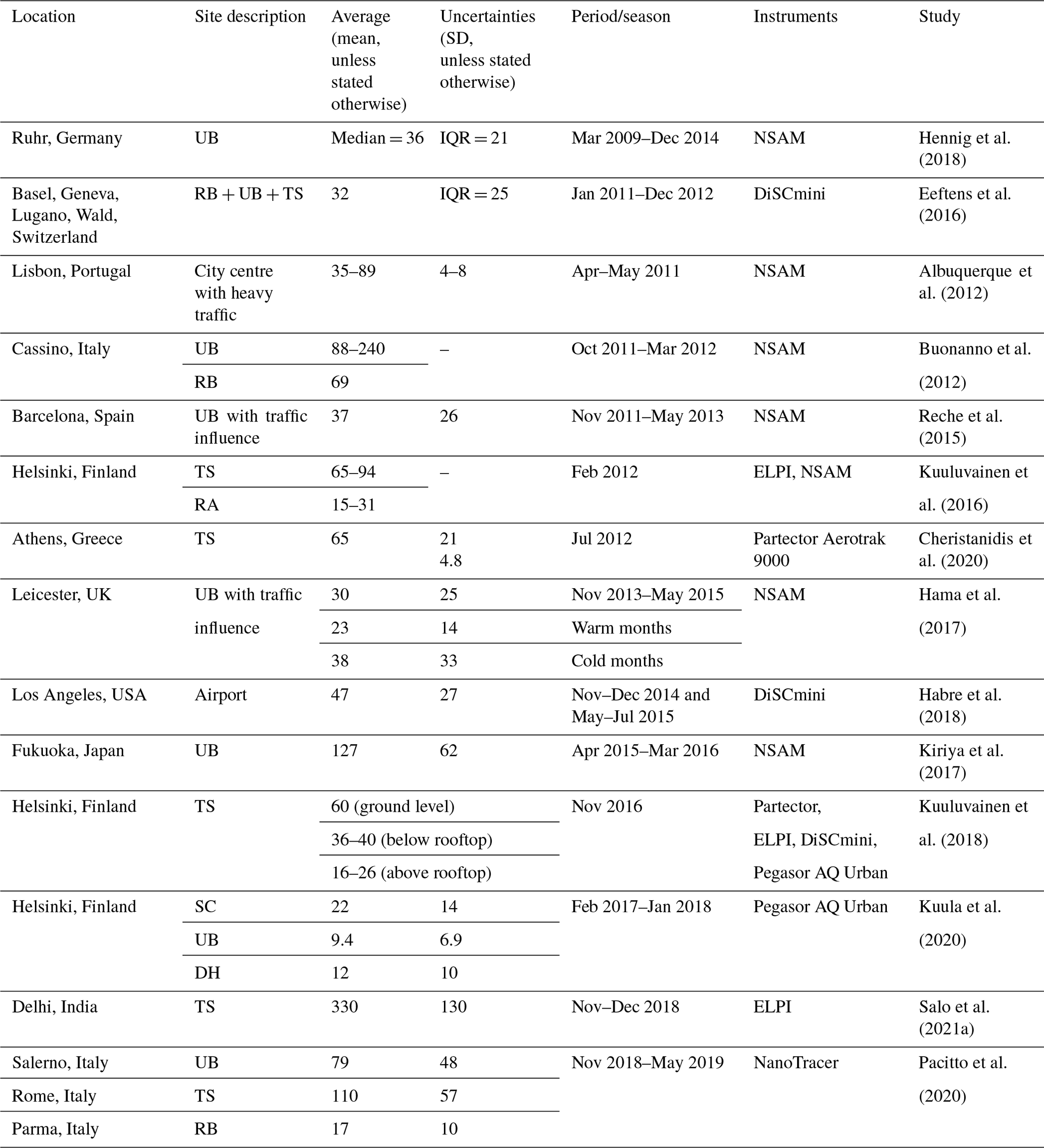
Apart from numerical computation method, LDSA could also be measured by accredited instruments. Diffusion charging based technique is a common approach where particles are charged with a unipolar corona charger (Fissan et al., 2006). This method enables measurement of ultrafine particles and, more specifically, the LDSA concentration with good accuracy (Todea et al., 2015) and stable performance in long-term measurements (Rostedt et al., 2014). A nanoparticle surface area monitor (NSAM) has been used for decades (e.g. Asbach et al., 2009; Hama et al., 2017; Kiriya et al., 2017; Hennig et al., 2018), and several other instruments and sensors, including DiSCmini, Testo Inc. (e.g. Eeftens et al., 2016; Habre et al., 2018) and Partector, Naneos Ltd. (e.g. Cheristanidis et al., 2020), and Pegasor AQ Urban, Pegasor Oy (e.g. Kuuluvainen et al., 2018; Kuula et al., 2020), using similar measuring techniques, were developed later on. Using these instruments in campaigns and continuous measurements, LDSA concentrations in the alveolar region and size distribution measurements in various environments have been reported across the globe in the past decade (Table 1). When comparing LDSA concentrations measured by different instruments, the instruments' limitations should be considered in experimental LDSA studies, which will be further discussed in Sect. 2.2.
Table 1Ambient LDSA of the alveolar region (in µm2 cm−3, corrected to two significant figures) reported in the last decade in chronological order of the measurement start. TS and RA represent traffic sites and residential areas, respectively. For the other acronyms, please see the methods section.
Although each of these methods is capable of measuring aerosol surface area concentrations, the corresponding uncertainties and cost hinder the widespread use in monitoring networks (Asbach et al., 2017). Even though the instruments are available, data can often be missing due to instruments maintenance and data corruption. Kuula et al. (2020) demonstrated high correlations of measured LDSA concentrations with black carbon (BC) and nitrogen oxide (NOx) in traffic environments. Traffic activities have been observed to be significant source contribution to the LDSA concentrations (Järvinen et al., 2015). A clear correlation was also found between the emission factors of exhaust plume BC and LDSA in on-road studies for city buses (e.g. Järvinen et al., 2019). These highly correlated relationships provide good grounds for estimating LDSA concentrations and short-term trends by the other pollutants measured at the same site with the use of a data-mining-based approach as statistical models. These statistical models can eventually turn into virtual sensors of LDSA after being validated even under the circumstances of no actual instrumental LDSA measurements. Due to the health effects LDSA has demonstrated, it is of great importance to researchers that continuous measurements of LDSA are available with the help of these virtual sensors via statistical models. A similar approach for sensor virtualisation of BC measurement has been studied in Fung et al. (2020).
A data-mining-based approach exploits statistical or machine learning techniques to detect patterns between predictors and dependent variables in the time series data. They do not demand in-depth understanding of air pollutant dynamics, but evaluation by experts is still required to determine whether the models work properly. Simple yet apprehensible models, such as multiple linear regression (MLR, e.g. Fernández-Guisuraga et al., 2016) and generalised additive models (GAMs, e.g. Chen et al., 2019), are commonly utilised as white-box models in air pollutant proxy studies. Furthermore, more sophisticated machine learning black-box models, such as artificial neural networks (ANNs, e.g. Cabaneros et al., 2019; Zaidan et al., 2019; Fung et al., 2021a), nonlinear autoregressive network with exogenous inputs (NARX, e.g. Zaidan et al., 2020) and support vector regression (SVR, e.g. Fung et al., 2021b), have been intensively investigated in recent years. They work better in terms of accuracy; however, they provide limited transparency and accountability regarding the outcomes (Rudin, 2019; Fung et al., 2021b).
Apart from model structures, the criteria of selecting variables in multipollutant datasets for model development have received considerable attention over the years, and a large number of methods have been proposed (Miller, 2002). Traditional methods, like stepwise procedures, which are a combination of forward selection and backward elimination (e.g. Liu et al., 2018b; Chen et al., 2019), can be unstable because they use a restricted search through the space of potential models, which eventually causes the inherent problem of multiple hypothesis testing (Breiman, 1996; Faraway, 2014). Another approach named regularisation has emerged as a successful method to reduce the data dimension in an automated way, yet it deals poorly with multi-collinear variables, for example, least absolute shrinkage and selection operator (LASSO, e.g. Fung et al., 2021b; Šimić et al., 2020), ridge regression (e.g. Chen et al., 2019) and ELASTINET (e.g. Chen et al., 2019). Criterion-based procedures, which choose the best predictor variables according to some criteria (coefficient of determination, residual, etc.), are sensitive to outliers and influential points but involve a wider search and compare models in a preferable manner. Examples are best subset regression (e.g. Chen et al., 2019), input-adaptive proxy (IAP, e.g. Fung et al., 2020, 2021b), etc. Hastie et al. (2020) compared some of the models using the three approaches and concluded that no single feature selection method uniformly outweighs the others. Despite the extensive research of feature selection methods, the inclusion of random effects together with the fixed effects as a linear mixed-effects (LME) model has received relatively little attention (e.g. Mikkonen et al., 2020; Tong et al., 2020) in air pollution research, let alone LDSA study in particular. This inclusion of random effects could acknowledge a possible effect coming from a factor where specific and fixed values are not of interest.
In this study, we combine the use of criterion-based feature selection method and the inclusion of random effects, and develop a novel input-adaptive mixed-effects (IAME) model to estimate alveolar LDSA concentrations, which is the first study of this context to our best knowledge. The description of LDSA measurements and the techniques of IAME model are outlined in Sects. 2 and 3, respectively. Section 4 presents the characteristics of alveolar LDSA, including its seasonal variability, weekend effect and diurnal pattern, in four types of environments. We also aim to investigate the correlation with other air pollutants. In Sect. 5, we evaluate the performance of the IAME proxy (LDSAIAME) with the measured alveolar LDSA by Pegasor AQ Urban (LDSAPegasor), ICRP lung-deposition-model-derived LDSA (LDSAICRP) and another modelled alveolar LDSA by IAP (LDSAIAP) as well as the benefits and implication of this alveolar LDSA model as virtual sensors. It should be noted that this study discusses LDSA in the alveolar region unless stated otherwise.
2.1 Measurement sites
We retrieved aerosol, gaseous and meteorological data from two types of measurement sites, i.e. street canyon (SC, 2017–2018) and urban background (UB, 2017–May 2018), in the Helsinki metropolitan area (HMA) described in more detail below. Data from detached housing (DH, 2017) and regional background (RB, 2017) sites were also included in the study to provide comparison and data from the background concentrations. Situated on a relatively flat land at the coast of Gulf of Finland, HMA has a land area of 715 km2 and population of about 1.13 million inhabitants. Helsinki can be classified as having a continental or marine climate depending on the air flows and the pressure system. Figure S1 and Table S1 in the Supplement show the detailed site description.
Street canyon (SC) site. The Mäkelänkatu urban supersite is operated by the Helsinki Region Environmental Services Authority (HSY, Kuuluvainen et al., 2018). The station is located 3 km from the city centre in a street canyon in the immediate vicinity of one of the main roads leading to downtown Helsinki. The street, with a speed limit of 50 km h−1, consists of six lanes and two tramlines. The annual mean traffic volume in 2018 per workday was 28 100 vehicles, 11 % of which were recorded as the heavy-duty vehicles. The traffic loads are especially high during rush hours at 08:00 and 17:00 LT (Fig. S2). The street canyon of width of 42 m is surrounded by rows of buildings 17 m high, which weaken the dispersion process of the direct vehicular emissions. All the inlets for the measuring devices are positioned approximately at a height of 4 m from the ground level.
Urban background (UB) site. The Station for Measuring Ecosystem-Atmosphere Relations III (SMEAR III, Järvi et al., 2009) in Kumpula, situated on a rocky hill 26 m above sea level, is about 4 km northeast of the centre of Helsinki. The surroundings of this urban background station are heterogeneous, constituting of residential buildings, small roads, parking lots, patchy forest and low vegetation from different directions. One main road (45 000 vehicles per workday) is located at a distance of 150 m east of the site. Trace gases and meteorological conditions are measured at heights of 4 and 32 m, respectively, at a triangular lattice tower, while aerosol measurements are conducted inside a container approximately 4 m above the ground. The site is co-operated by Finnish Meteorological Institute (FMI) and the University of Helsinki (UHEL).
Detached housing (DH) site. Three measurement stations, Rekola (DH1), Itä-Hakkila (DH2) and Hiekkaharju (DH3), were chosen since they represent a suburban residential area surrounded by detached houses. These sites are mainly affected by the wood combustion emissions from residential activities, especially in cold weather conditions. Emissions from traffic sources also account for a small portion of the whole pollution. It is estimated that 90 % of the households burn wood to warm up houses and saunas, less than 2 % of which use wood burning as the main heating source in detached houses in HMA (Hellén et al., 2017).
Regional background (RB) site. The RB site is located about 23 km away from the Helsinki city centre in Luukki, surrounded by a wooded outdoor recreational area right at the edge of the greater Helsinki golf course. The measuring station is in an open place away from busy traffic routes and large point sources. As a result, this site can represent background concentration levels outside the urban area without any main local sources.
2.2 Instruments
LDSA measurements. The sensor unit and the core of the Pegasor AQ Urban are practically another instrument called a Pegasor Particle Sensor M (PPS-M) sensor (Pegasor Oy, Finland), originally designed for automotive exhaust emission measurements (e.g. Maricq, 2013; Amanatidis et al., 2017). The operation of the sensor is based on diffusion charging of particles and the measurement of electric current without the collection of particles. The diffusion charging of particles is carried out by a corona-ionised flow that is mixed with the ambient sample air in an ejector diluter inside the sensor. The performance of the Pegasor PPS-M sensors for long-term ambient measurements has been improved after they were tested in Helsinki (Järvinen et al., 2015) and Beijing (Dal Maso et al., 2016). The suggestions have been considered for the design of the current form of the Pegasor AQ Urban in this study.
The Pegasor AQ Urban (dimensions: 320 mm × 250 mm × 1000 mm), which consists of a weatherproof cover, clean air supply and the above-mentioned Pegasor PPS-M sensor, has been designed such that its response to LDSA is not to be subjected to meteorological fluctuation for outdoor operation. The sampling lines and the sensor unit are heated to 40 ∘C above the ambient temperature to (1) dry the aerosol sample, (2) prevent interference from humidity and (3) prevent any water condensation inside the sensor. Kuuluvainen et al. (2016) used two Pegasor AQ Urban devices during a 2-week period at an urban street canyon and an urban background measurement station in Helsinki, Finland, whereas Kuula et al. (2019) later used the instruments in a 3-month campaign at the same urban street canyon station. These studies demonstrated that the output signal of the Pegasor AQ Urban correlated well with other devices measuring LDSA concentrations such as the Partector and DiSCmini. Kuula et al. (2020) further validated the accuracy and stability of Pegasor AQ Urban at the street canyon station by comparing the measured values of 1 full year with differential mobility particle sizer (DMPS) reference instruments (R2=0.90, RMSE = 4.1 µm2 cm−3). The internal precision of Pegasor AQ Urban is ±3 %, but this was not tested prior the campaign. The instrument is optimised to measure the alveolar LDSA concentrations of particles in the ∼ 10–400 nm size range. Pegasor AQ Urban tends to underestimate LDSA of particles larger than about 400 nm. In typical urban environments, most of the particles from local combustion sources are in the size below the threshold (Asbach et al., 2009; Kuuluvainen et al., 2016; Pirjola et al., 2017), generated vastly by anthropogenic sources such as vehicular exhaust emissions (Karjalainen et al., 2016) and residential wood combustion (Tissari, 2008), which typically produce large amounts of small particles. However, the impact of larger particles (>400 nm) on alveolar LDSA might be significant, for example, in HMA during PM2.5 long-range-transport episodes or when there are many particles from very low-quality residential burning in detached housing areas (Pirjola et al., 2017). The regional background source in very polluted regions (e.g. Delhi, Salo et al., 2021a; mining environments, Salo et al., 2021b) could be another reason for the significant impact of larger particles. This limitation of Pegasor AQ Urban should be considered when it comes to data analysis in Sects. 4 and 5.
Aerosol measurements. A DMPS in combination of a differential mobility analyser (DMA) and a condensation particle counter (CPC) measure aerosol size distribution (Kulkarni et al., 2011). A Vienna DMA and Airmodus A20 CPC (measurements of particle size range 6–800 nm) were used at the SC site, while a twin DMPS (Hauke-type DMA and TSI model 3025 CPC and Hauke-type DMA, and TSI Model 3010 CPC, merged particle size range of 3–1000 nm) was used at the UB site. Both instruments make use of the bipolar charging of aerosol particles, followed by classification of particles into size classes according to their electrical equivalent mobility. In addition to particle size distribution, total particle number concentration (PNC, in cm−3) was calculated by summation. Particle mass concentrations with a diameter less than 2.5 µm (PM2.5, in µg m−3) and less than 10 µm (PM10, in µg m−3) were measured continuously with the ambient particulate monitor TEOM 1405 at the SC site and TEOM 1405-D at the UB site. Black carbon (BC, in µg m−3) mass concentration was measured by a multi-angle absorption photometer (MAAP) Thermo Scientific 5012 with a PM1 inlet. The measured absorbance was converted to BC mass concentration by using a fixed 6.6 m2 g−1 mass absorption coefficient at a wavelength of 637 nm. PM2.5, PM10 and BC were recorded in µg m−3.
Ancillary measurements. Trace gas concentrations (in ppb), including nitric oxide (NO), nitrogen dioxide (NO2), their combined nitrogen oxide (NOx), ozone (O3) and carbon monoxide (CO), were determined with a suite of gas analysers. In addition, supporting meteorological variables, including air temperature (Temp), relative humidity (RH), air pressure (P), wind speed (WS), wind direction (WD) and photosynthetically active radiation (PAR), were measured at SC and UB. Figure S3 shows the meteorological conditions during the measurement period. A list of collected variables is shown in Table S2.
3.1 Data pre-processing
The collected data were quality checked by the corresponding operating organisation (HSY, FMI and UHEL). No additional pre-processing was done for general analysis. For proxy development, outliers due to potential measurement errors were detected (SC: 0.73 %; UB: 0.99 % overall) by using the interquartile range (IQR) rule, which is applicable for non-Gaussian distribution sample. We calculated the cutoff for outliers as 2 times the IQR, subtracted this cutoff from the 25th percentile and added it to the 75th percentile to give the actual limits on the data. We applied a natural logarithm transformation to all the skewed-distributed aerosol and trace gas measurements in order to keep the distribution of each parameter following a normal distribution. Since wind direction is a circular variable, it is resolved into north–south (WD–N) and east–west (WD–E) vector components by trigonometric functions.
3.2 Size-fractionated lung-deposited surface area (LDSAICRP)
Alveolar deposition fraction (DFAL) as a function of particle size with the unit density is determined with the ICRP Human Respiratory Tract Model by the following equation (ICRP, 1994):
where dp is the aerodynamic diameter (µm) of spherical particles with the unit density (1 g cm−3). The equation is determined in two parts with respect to the two different peaks in the deposition curve in Fig. 1. The peak near the size of 20 nm can be approximated to represent the Brownian deposition, whereas the peak between 1 and 2 µm represents the inertial deposition. From the particle number size distribution, we calculated the particle surface area distribution assuming each particle is monodisperse sphere of standard density at standard conditions. By Eq. (1), a deposition factor for each particle size bin (26 size bins at SC and 49 at UB) were calculated. Size-fractionated LDSA was then computed by multiplying the surface area concentration with DFAL in the corresponding size class. Total LDSA calculated by the ICRP lung model (LDSAICRP) can be obtained by summing up the all the size-fractionated LDSA values (Hinds, 1999). In this study, the alveolar LDSAICRP was calculated based on DMPS measurements in SC and UB. Thus, while the alveolar LDSA measured by Pegasor (LDSAPegasor) represents the ∼ 10–400 nm size range, the alveolar LDSAICRP represents the 6–800 and 3–1000 nm size ranges in SC and UB, respectively.
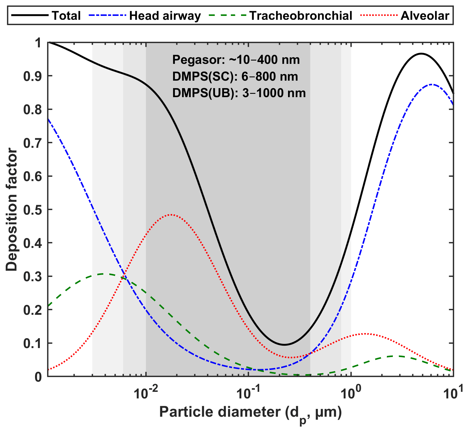
Figure 1Lung deposition factor of a spectrum of particle size distribution based on the equation (ICRP, 1994). The solid black line represents the total deposition factor, while the dotted blue, green and red lines refer to deposition factor in head airway, tracheobronchial and alveolar regions, respectively. Pegasor AQ Urban measured the alveolar LDSA concentration of particles in the ∼ 10–400 nm size range (dark grey). DMPS at SC and UB were used to calculate alveolar LDSA in selected size fractions in the 6–800 and 3–1000 nm size ranges, respectively
3.3 Novel IAME model
The IAME model is a combination of IAP and LME models. IAP was first introduced by Fung et al. (2020) and has been demonstrated to be reliable and flexible for filling up missing values by taking input variables adaptively with robust ordinary least-square regression models. IAP has been able to estimate BC concentration by other air quality indicators with a satisfactory performance in two different categorised urban environments: street canyon (adjusted R2 = 0.86–0.94) and urban background (adjusted R2 = 0.74–0.91). Some models outperformed IAP in accuracy performance, but its transparent model structure and ability to impute missing values still make it a preferred option as a virtual sensor (Fung et al., 2021b).
In this study, we primarily stuck to the strength to select input variables adaptively with the introduction of mixed effects. The mixed-effects approach is a generalisation of the linear model that can incorporate both fixed (i.e. causing a main effect and/or interaction) and random effects (i.e. causing variance and/or variability in responses), allowing the account of several sources of variations (Chudnovsky et al., 2012). As seen in Fig. 2, we picked the direct air pollutant measurement from the station (variables of high correlation: PM2.5, BC and NO2 and other supporting variables: PM10, O3, NOx, NO, CO and PNC) and meteorological data of higher correlation (Temp, RH, P, PAR, WS, WD–N, WD–E) as the fixed variables because the air pollutants can indicate the sources of LDSA which largely come from combustion and meteorological data could influence the dispersion and dilution of LDSA. They are the most direct factors to the fluctuation of LDSA concentrations. Due to the strong seasonal variation, weekend effects and diurnal pattern in urban air pollutant concentrations (Fung et al., 2020), the variance in responses might depend on the time indicators that are not the primary cause of the concentration variability, but they indirectly alter human-induced activities, such as traffic amounts. To take them into account, we created three hierarchical time subgroups (12 months of the year, 7 d of the week and 24 h of the day) as the inputs of random effect variables.
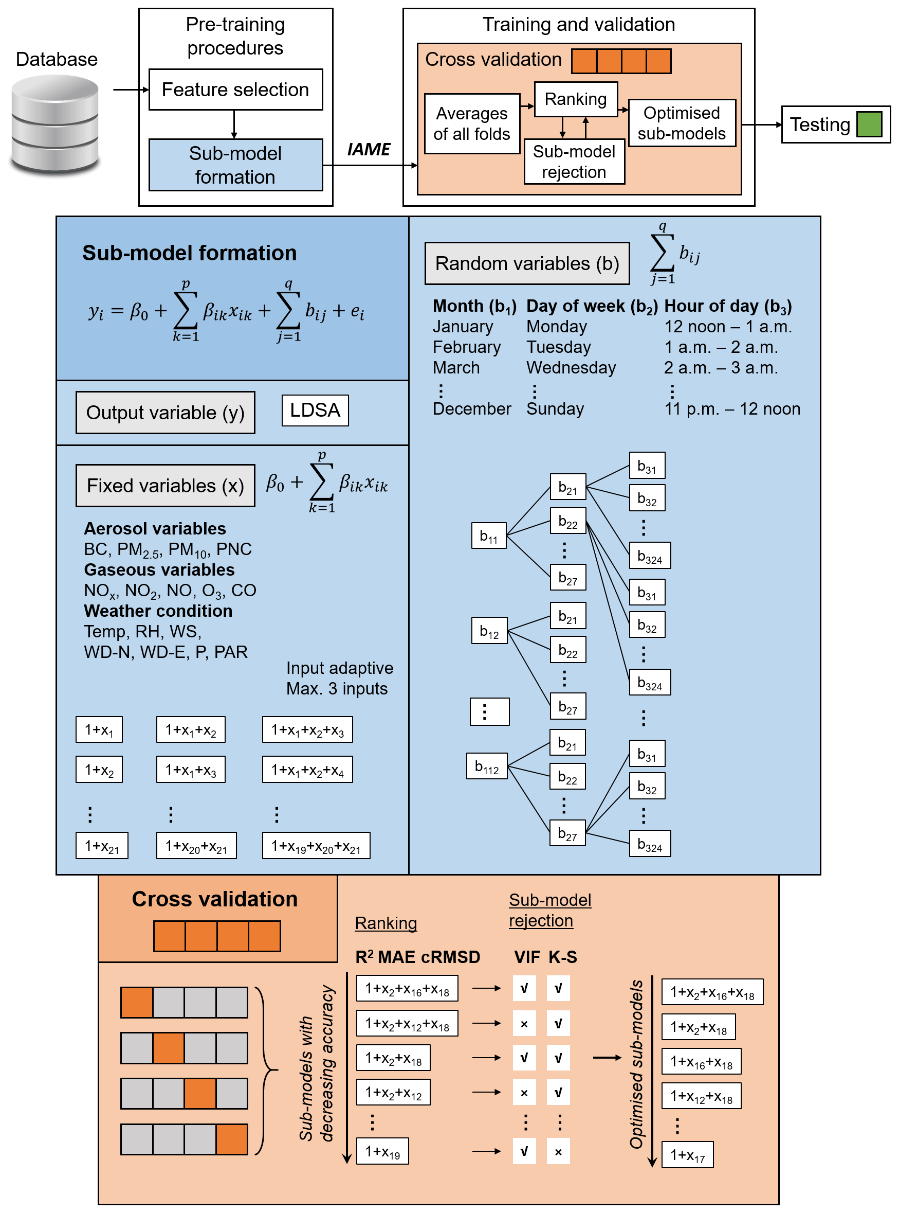
Figure 2The block diagram of the proxy procedures (top). The blue and orange blocks are explanatory notes to the sections of submodel formation and cross validation, respectively.
The regression equation of IAME is similar to the equation of IAP, except that IAME includes additional intercepts term for random effects as below:
where yi is the ith estimated LDSA concentration. The first term on the right β0 indicates the fixed intercept of the equation. The second term represents the total contribution by the direct measurement of variable x as fixed effects with a slope β at each data point i. A maximum of three inputs from the total 16 fixed variables are selected to from 696 submodels (Fig. 2). The inputs for random effects are indicated by b as intercepts of the corresponding three hierarchical subgroups. A Gaussian error term is indicated by e. The explanation of Eq. (2) is visualised in Fig. 2.
One of the assumptions of LME models is that the random effects, together with the error term, have the following prior distribution:
where D is a q-by-q symmetric and positive semi-definite matrix, parameterised by a variance component vector θ, q is the number of variables in the random-effects term, and σ2 is the observation error variance. We use an optimiser, restricted maximum likelihood, commonly known as ReML, with the value as the relative tolerance on gradient of objective function and as absolute tolerance on step size. The use of ReML over the conventional ML could produce unbiased estimates of variance and covariance parameters (Lindstrom and Bates, 1988).
After the submodel formation, the dataset was randomly divided into five portions. In total, 80 % of the data were allocated for 4-fold cross validation to remove variance of accuracy. The results of all the folds were averaged and the submodels were ranked by several evaluation metrics, which were further demonstrated in Fig. 2 and described in Sect. 3.4. Some of the submodels were subject to rejection under two conditions: (1) strong multi-collinearity among the fixed parameters (variance inflation factor (VIF) > 5) and (2) violation of the normality assumption of residuals also known as heteroscedasticity (fail in Kolmogorov–Smirnov (K–S) test, p<0.05). Based on the situation of missing data, the automatised IAME model would search for the best submodel option from the ranking chart. Hence, each data point might be estimated differently depending on the available data. The number of data points being estimated by each submodel was reported to show their frequency of usage.
3.4 Evaluation metrics
In order to evaluate the model performance quantitatively, we used the following metrics:
where yi and are ith measured data point and estimated variable by the model, respectively. and are the expected value of the measured and modelled dataset, respectively. N is the number of complete data input to the model. The coefficient of determination (R2) is a measure of how close the data lie to the fitted regression line. It, however, does not consider the biases in the estimation. Therefore, we further validated the models with mean absolute error (MAE) and centred root-mean-square difference (cRMSD), where MAE measures the arithmetic mean of the absolute differences between the members of each pair, whilst cRMSD calculates the square root of the average squared difference between the forecast and the observation pairs. cRMSD is more sensitive to larger errors than MAE. Furthermore, together with cRMSD, Pearson correlation coefficient (r) and normalised standard deviation (NSD) of the modelled dataset are also studied. r describes the correlation between the measured and modelled data, whereas NSD measures the relative spread of the data. Due to their unique mathematical relationship, the three metrics can be portrayed on Taylor's diagram, which has been used for submodel selection purpose. We ranked our submodels first by R2, followed by MAE and cRMSD. r and NSD serve as additional evidence when we explain the model performance.
3.5 Two-sample t tests
We assessed the temporal and spatial impact on the IAME model by comparing the means of absolute differences between the hourly measured and modelled LDSA in different time windows at both stations. Two-sample t tests were performed on the two populations of absolute differences above-mentioned to determine whether the difference between these was statistically significant. A significance level α of 5 % was chosen as the probability of rejecting the null hypothesis when it is true, denoted as p.
4.1 General characteristics of LDSAPegasor in the Helsinki metropolitan area
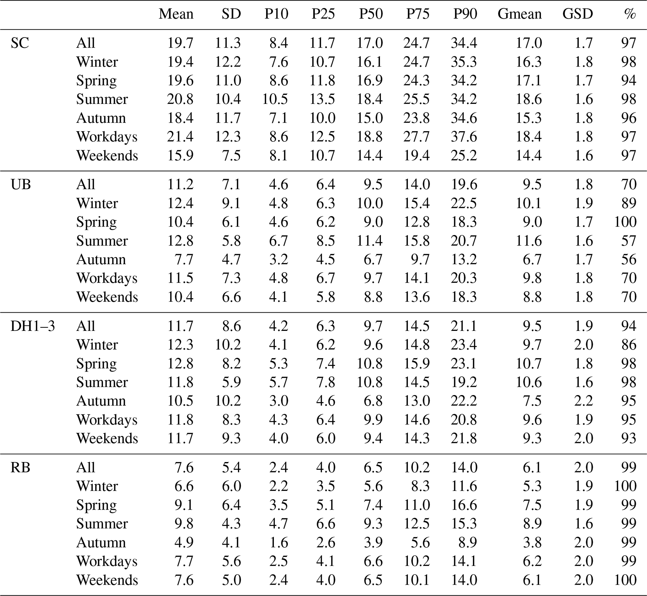
The annual mean alveolar LDSA concentrations at four station types, SC (2017–2018), UB (2017–May 2018), DH (2018) and RB (2018), were 19.7 ± 11.3, 11.2 ± 7.1, 11.7 ± 8.6 and 7.6 ± 5.4 µm2 cm−3, respectively (Table 2). The DH and RB site were included to give more substantial interpretation of data because the LDSA concentrations at RB can be viewed as background measurements and the local LDSA increments in HMA can be represented by the LDSA at the hotspot measurement site subtracted by the LDSA at the RB site. The time series of LDSA concentrations at the SC and the UB site were presented in Figs. 3 and S4, where the missing data of LDSA for the whole measurement period were 3 % and 30 %, respectively. When comparing with the same site type in other cities around the globe, LDSA concentrations detected in HMA were the lowest among the European cities with reported values. While some literature also reported LDSA at tracheobronchial region, most just considered LDSA at alveolar, which is considered to bring the most harm to human lungs, as shown in Table 1.

Figure 3Time series of the selected air pollutant parameters (first to end row: LDSA (µm2 cm−3), BC (µg m−3), NOx (ppb), PM2.5 (µg m−3) and PNC (cm−3)) at the Mäkelänkatu SC site during the measurement period from 1 January 2017 and 31 December 2018. Each bar represents a period of 2 weeks where the shaded diamond marker is the median and the vertical error bars are the 25th and 75th percentiles. Seasons are thermally separated.
Table 2Descriptive statistics of alveolar LDSA concentrations (µm2 cm−3) at SC (2017–2018), UB (2017–May 2018), DH1–3 (2018) and RB (2018) sites. The mean (column 3), standard deviation (SD, column 4), 10th, 25th, 50th, 75th and 90th percentiles (P10, P25, P50, P75 and P90, columns 5–9), geometric mean (Gmean, column 10) and geometric standard deviation (GSD, column 11) of the concentrations are corrected to one decimal place. The percentage of valid data in the reported measurement period is shown in column 12.
The diurnal pattern of LDSA at RB was not observable on workdays or over weekends (Fig. 4, upper panel). The relatively low variability can be explained by the scarcity of human activities. We can then regard the LDSA at RB as the background concentrations mainly influenced by the regionally and long-range-transported aerosol and meteorological variation (see Luoma et al., 2021; Jafar and Harrison, 2021). The concentration at RB was stable throughout the different hours of day; therefore, the diurnal pattern of LDSA concentration was apparently indistinguishable between the measured concentration and the local increments. At the UB and DH sites, the magnitudes and the patterns of the average hourly LDSA concentrations during workdays were comparable, and both showed bimodal curves: one peak at 06:00–09:00 LT, the other at 21:00–23:00 LT. The former had a larger peak during the morning peak hour because of the vehicular emissions (Timonen et al., 2013; Teinilä et al., 2019), while the latter had a larger peak in the evening attributed mainly to the residential burning (Hellén et al., 2017; Helin et al., 2018; Luoma et al., 2021). Over weekends, the peaks in the morning were not identifiable and the evening peaks were amplified due to enhanced human activities. A similar diurnal variation in residential areas was observed for BC emitted by residential combustion by Helin et al. (2018). At the SC site, the morning peak on weekends was not obvious because of the lack of work-related traffic. It appears that a similar bimodal curve can be seen during workdays, but the evening peak was seen during the evening traffic rush hour around 16:00–18:00 LT. The reason was that the main contributor of LDSA at the SC site was traffic and combustion processes and the diurnal variability mainly depended on the citizen's movement by vehicles in the city. During weekends, the average hourly LDSA concentrations were the minimum at 05:00 LT and they increased and remained at a high level at 17:00 LT until late at night. The level of LDSA concentrations at DH was comparable with that at the UB site. However, the amplitude of the evening peak was higher than that of the morning peak both on workdays and weekends due to elevated residential combustion.
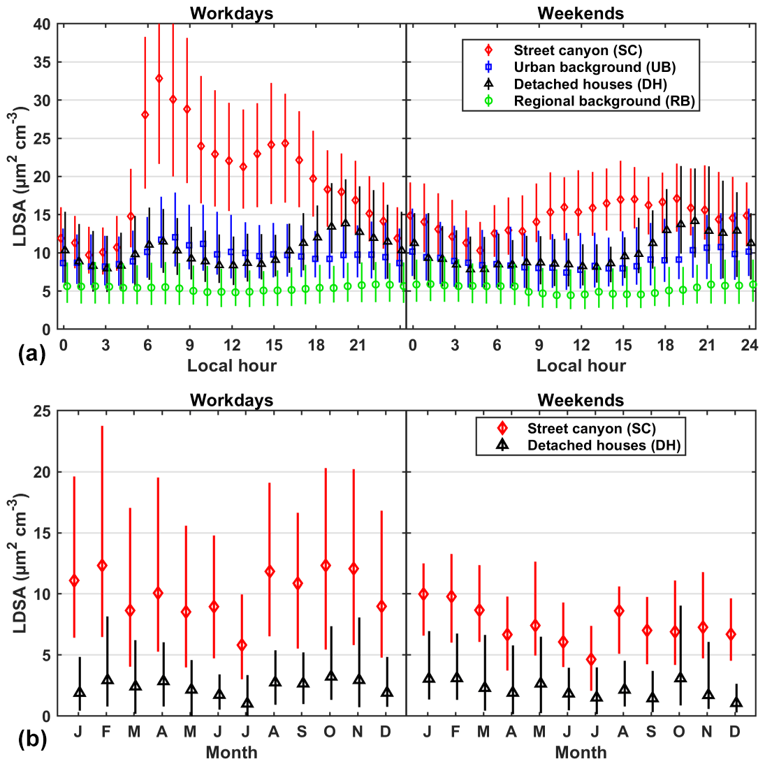
Figure 4(a) Diurnal cycles of LDSA concentrations (µm2 cm−3) at the SC (red diamond, 2017–2018), UB (blue square, 2017–May 2018), DH1–3 (black triangle, 2018) and RB sites (green circle, 2018) on workdays and weekends with error bars of 25th and 75th percentiles. (b) Monthly averages in the year 2018 of local LDSA increments at the SC (red diamond) and DH1–3 (black triangle) sites (LDSA concentration at the hotspot site minus LDSA at the RB site) on workdays and weekends with error bars of 25th and 75th percentiles.
However, the monthly variability of background measurements at the RB site was stronger compared to the diurnal pattern, and the calculation of local increment was necessary (e.g. Jafar and Harrison, 2021). With no intense point sources, the variations at RB were probably due to horizontal dispersion and advection of aerosol particles and vertical dilution controlled by the boundary layer dynamics. Based on the monthly frequencies of backward trajectory by the NOAA Hybrid Single-Particle Lagrangian Integrated Trajectory (HYSPLIT) model (Rolph et al., 2017, Fig. S5), pollutants could be originating 600 km away from Helsinki within 24 h in the winter. In the summer, when solar radiation was persistently stronger, the boundary layer became elevated due to surface heating and associated thermal turbulence. This turbulence would dilute the concentration of pollutants at the surface. Another plausible reason could be the higher regional and long-range-transported LDSA in the summer, as demonstrated by Kuula et al. (2020) and Barreira et al. (2021). The lower panel in Fig. 4 shows the LDSA local increments after subtraction of the LDSA concentrations at the RB site. For instance, the local LDSA increments at DH are the highest in the winter probably due to local small-scale wood combustion (and traffic). However, without subtracting the background concentrations, the LDSA concentrations at DH were higher in the summer than in the winter (due to high regional background concentrations in summer), as was observed also by Kuula et al. (2020). This piece of evidence can help in the source apportionment. The variations of diurnal and seasonal LDSA for all sites are visualised in Fig. S6.
4.2 The connection between LDSA and other parameters
Alveolar LDSA concentration, as a single number, comprises particles across the whole particle size spectrum measured (e.g. Pegasor AQ Urban ∼ 10–400 nm). In HMA, the two local main sources of particles contributing to LDSA are vehicular combustion and residential wood combustion emissions. Upon the two combustion processes, particles of different sizes and different gaseous pollutants are emitted. A study by Lamberg et al. (2011) has shown that the geometric mean diameter of residential wood combustion is typically 70–150 nm, whereas Barreira et al. (2021) presented that the typical particle size for vehicular combustion can be smaller than 50 nm. By calculating the proportion of LDSA with respect to different pollutant parameters such as BC, NOx, PNC (dominated by UFP) and PM2.5, we could identify the relative contribution of LDSA across the hour of the day (Fig. S7 for workdays and Fig. S8 for weekends). Whereas the ratios could partly tell the relative contribution of LDSA in that certain hour, they are also dependent on various factors that include the different properties of each parameter (e.g. the lung deposition factor for LDSA) and the time-dependent increase in particle size (e.g. new particle formation) which are not the focus of this paper. Since vehicular combustion emits smaller particles which elevate the LDSA concentration but meanwhile do not substantially influence the value of PM2.5 (e.g. Salo et al., 2021a), LDSA PM2.5 had a diurnal pattern similar to the LDSA concentrations which peaked in the morning rush hour during workdays. Conversely, LDSA BC, LDSA PNC and LDSA NOx had a low ratio value in the morning rush hour. This can be explained by the fact that vehicular combustion caused high concentrations of BC, PNC and NOx (Reche et al., 2015) compared to its contribution to LDSA concentration. In other words, the role of regional background was higher for LDSA compared to those of NOx, BC and PNC. At the UB site, the average LDSA BC at all hours remained at a constant level in the winter, while the variability of the ratio was much higher in the summer. The general LDSA PNC ratio at UB was steadily 2–3 times higher than that at all hours in all seasons because the proportion of larger particles at UB was usually higher than SC. This large variability again validated the heterogeneity of source of LDSA at UB.
The integrated alveolar LDSA with a various size ranges was calculated to explore the correlation of size-fractionated LDSA and other parameters in our multipollutant dataset. No single fractionated LDSA correlated well with meteorological parameters at both sites (Fig. 5). Out of all fractions, alveolar LDSA of the whole spectrum (LDSA6–800) and LDSA250–400, which explained majority of LDSA, correlated best with other air pollutants. In general, alveolar LDSA had a high correlation with BC. BC correlated the best with LDSA100–250 (r=0.84), which was in alignment with the reported values from previous literature (Gramsch et al., 2014; Ding et al., 2016). As expected, PM2.5 showed better correlation with the LDSA of larger particles (r = 0.68–0.76) because larger particles contribute more to PM2.5 mass concentration values. In the meantime, PM10 had a fair correlation with all selected size bins. NO2 correlated highly with LDSA of smaller particles (r = 0.69–0.77), indicating the dominant role of local traffic exhausts. CO had a higher correlation with LDSA of 400–800 nm (r=0.64) since CO concentrations were more affected by regionally transported pollutants. O3 had a fair correlation with LDSA of all sections (r = 0.30–0.43) because the formation of O3 is mostly secondary and the chemical interactions with pollutants are more complicated than the other compounds. In general, the correlations of LDSA with other air pollutant parameters were higher at the SC site than that at the UB site (Fig. S9). The high correlations of LDSA with BC, PM2.5 and NO2, which agreed with the results by Kuula et al. (2020), proved the possibility of developing a model to estimate LDSA concentrations.
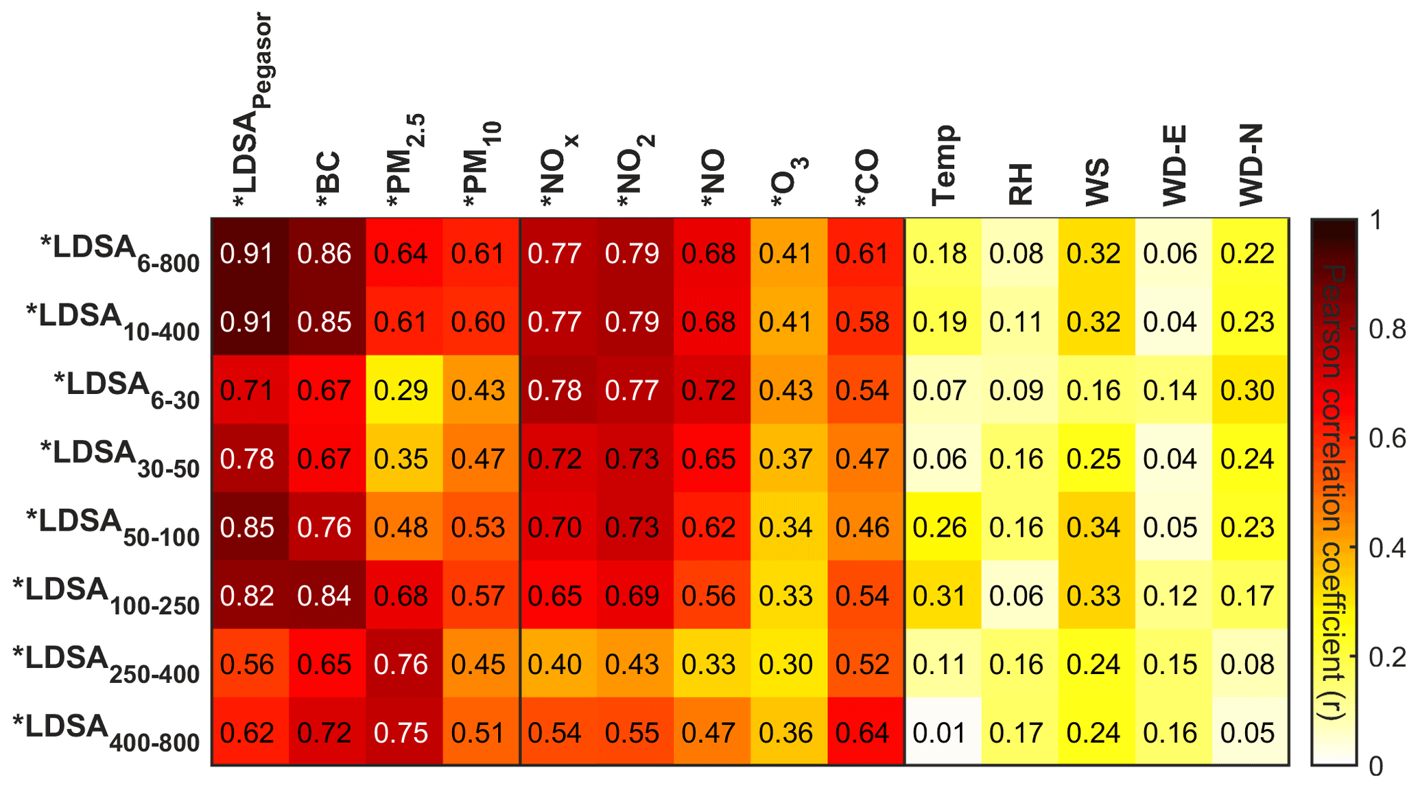
Figure 5Heatmap showing Pearson correlation coefficient (r, corrected to two significant figures) of LDSA of different particle size sections (in nm) by ICRP lung deposition model and the other air pollutant parameters at the Mäkelänkatu SC site. Dark red indicates a high correlation, while pale yellow indicates a low correlation. Parameters with an asterisk represent a natural logarithm. LDSAPegasor represents the measured LDSA concentrations.
5.1 Submodel diagnostics
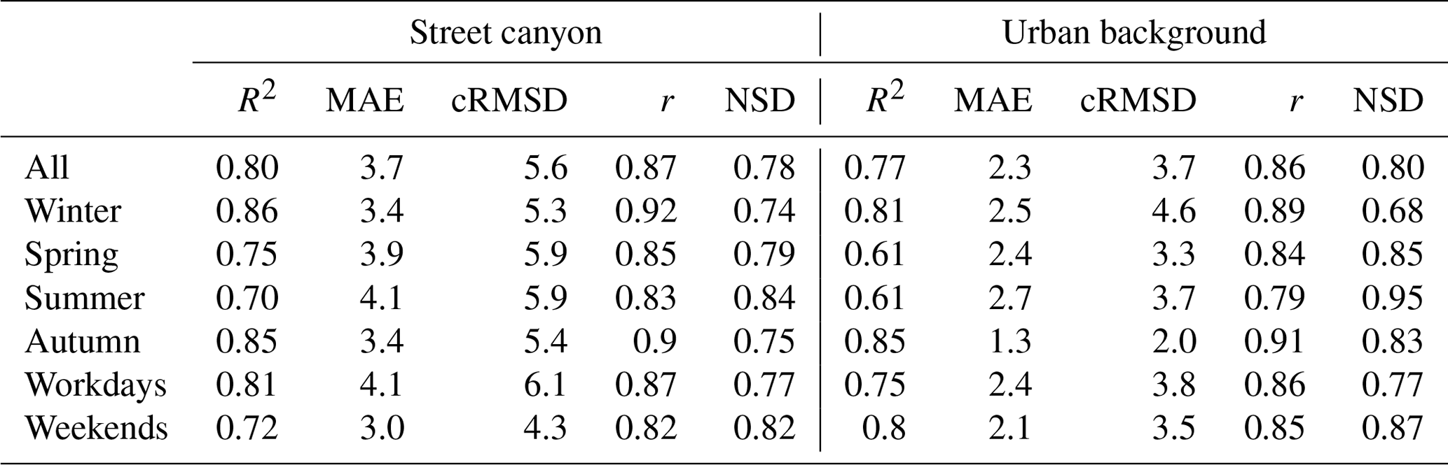
Following the evaluation attributes described in Sect. 3.4, Table 3 depicts the descriptive statistics of the overall model evaluation on its testing set. The overall model at the SC site was able to explain 80 % of the variability of the testing set of the measured data. The R2 in the winter was 0.86, being the highest, while the worst R2 was shown in the summer, i.e. 0.70. The MAE and cRMSD were the smallest during weekends with R2 not particularly high (R2=0.72) probably because the LDSA concentration itself was relatively low in that period. The overall performance was generally worse in UB in terms of R2, except during weekends that R2 is 10 % higher.
Table 3The evaluation attributes by IAME model at the SC and UB sites, corrected to two significant figures.
For individual submodels, their performance could be seen on the Taylor diagram in Fig. 6 (Taylor, 2001). Each marker represents one submodel, the contribution of which to the outcome of the final model is displayed in various colours. The submodel performance can be evaluated by the distance of the submodel marker and the red point, which represents the reference station, i.e. the perfect model. The location of each marker indicates its individual performance in terms of r (blue contours), cRMSD (green contour) and NSD (black axis). At the SC site, the narrow distribution of the submodels on the Taylor diagram gives a clue that they were very similar in terms of model performance of LDSA estimation. The five mostly used submodels were concentrated within the region where r was 0.85–0.87, cRMSD was 5.67–5.77 µm2 cm−3 and NSD was 0.75–0.79 (Table 4). The values of their evaluation metrics were close to each other where R2 and MAE differed in the narrow range of 10 % (R2 = 0.72–0.74, MAE = 3.8 µm2 cm−3). It infers that if one metric was prioritised over another, the rank of the submodels can be greatly different. Although no individual submodels showed r greater than 0.9, the overall model comprising the outcomes by all the submodels remained high (R2=0.80, MAE = 3.8 µm2 cm−3). The best submodel was also the most used one, which accounted for 81 % of the total data points, while the two succeeding submodels constituted another 16 %. This also indicates that the input adaptivity function of the suggested method supplemented 19 % of the estimates, which would be a missing estimate if a single model with fixed predictor variables was used. Four out of the five most used submodels contain BC as an input predictor with the combination of the other two air pollutants or meteorological parameters. This was in line with the high correlation of LDSA with BC (r=0.84, Fig. S9). In the event that BC is missing at a certain time stamp, the submodel without BC as an input could be used. It further supports the input-adaptive function.
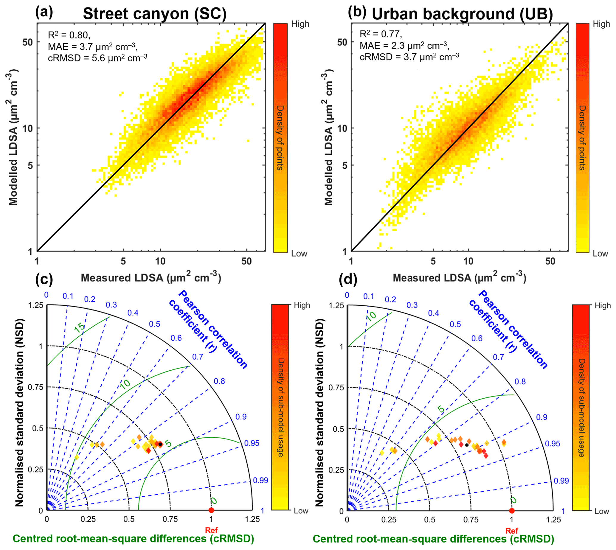
Figure 6Panels (a) and (b) show the scatter plots of modelled LDSA against the measured LDSA at the (a) Mäkelänkatu SC site and (b) Kumpula UB site. Hues of colours represent the density of points on the figure. Panels (c) and (d) show the Taylor diagrams (Taylor, 2001) at the (c) Mäkelänkatu SC site and (d) Kumpula UB site. Each diamond marker in the Taylor diagrams represents each submodel used in the final estimation by IAME (solid black dot), compared with the reference data (solid red dot). Hues of colours represent how frequently the submodel was used.
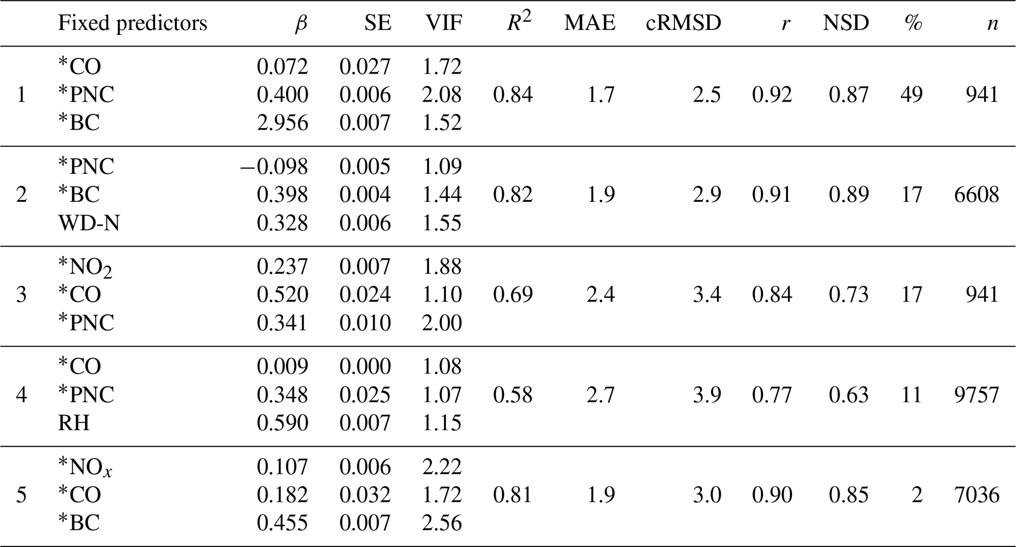
Table 4The five most successful submodels at the SC site. The table shows only the fixed predictors with their coefficient (β, all p<0.05) and corresponding standard error (SE). The variance inflation factor (VIF) among the fixed predictors is also shown for the five submodels. The evaluation attributes of the submodels are shown in columns 6–10. The percentage of the submodel usage and the number of data points (n) are shown in columns 11 and 12. The natural logarithm is taken for parameters with an asterisk (*).

At the UB site, the submodel performance was more scattered on the Taylor diagram (Fig. 6). The five most used submodels had varying metrics (r = 0.77–0.92, cRMSD = 2.5–3.9 µm2 cm−3 and NSD = 0.63–0.89; see Table 5). Although some showed exceptionally good performance, the overall model had a slightly worse performance than that in street canyon. The best submodel estimated 49 % of the total measurement, followed by 17 %. The third and fourth most used submodels, which formed up to 30 % of the estimates, had rather moderate performance (R2=0.58 and 0.69). Considering all possible outcomes, the overall model was still able to explain 77 % of the total variance. Despite the fair linear correlation with LDSA, CO (r=0.26) and PNC (r=0.71) dominated in the top five used submodels. This could be explained by the fact that the source of CO can well cover the missing piece that PNC was unable to account for LDSA. BC, NOx and meteorological parameters, like RH and WD–N, were also involved in the final LDSA estimation.
By checking the variance inflation factor (VIF) of all 696 submodels, 4.6 % and 2.2 % were rejected respectively. The higher rejection rate at SC can be explained by the fact that some of the predictor variables were highly correlated to each other and the inclusion of them would result in an inflation of multi-collinearity of the submodel, from which biases arose. At UB, since the source of LDSA was more varied and the correlation of LDSA with other pollutants was generally lower, the probability of the VIF of the individual submodels exceeding the threshold was lower.
Table 5The five most successful submodels at the UB site. The table shows only the fixed predictors with their coefficient (β, all p<0.05) and corresponding SE. The VIF among the fixed predictors is also shown for the five submodels. The evaluation attributes of the submodels are shown in columns 6–10, corrected to two significant figures. The percentage of the submodel usage and the number of data points (n) are shown in columns 11 and 12. The natural logarithm is taken for parameters with an asterisk (*).
5.2 Temporal difference in comparison with other models
Figure 7 presents the comparison of measured LDSA (LDSAPegasor), deposition-model-derived LDSA (LDSAICRP) and the LDSA modelled by IAP and IAME (LDSAIAP and LDSAIAME) as a time series plot between 14 and 28 February 2017. This particular time window was selected because it had the least data gaps for all the respective instruments at both sites. This figure during this period can also showcase the difference in magnitudes of the diurnal shape over workdays and weekends (shaded regions in Fig. 7). At both sites, both IAP and IAME underestimated the peaks when the change of the measured LDSA concentration was sudden and relatively large. However, this limitation did not diminish much of the usefulness of the models as virtual sensors as the models were still able to generally catch up with the diurnal cycle of the measured data. Despite the small difference observed in the figure, the dotted blue line representing LDSAIAME often stays closer to the measured LDSA concentration (black line). When we smoothed out all the estimates at each hour, the ability of IAME to catch the morning peak on workdays was much better.
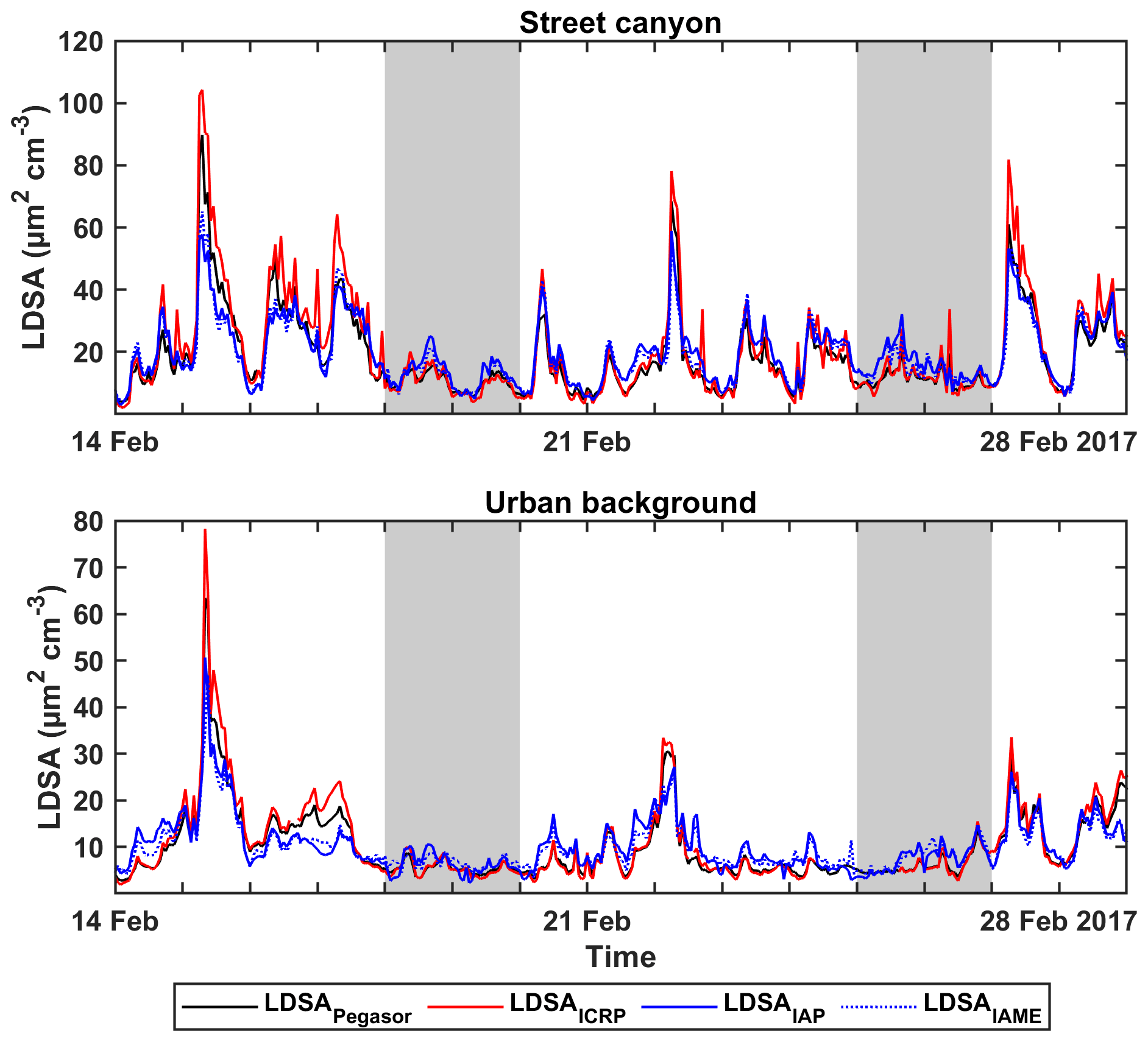
Figure 7Time series of measured LDSA (LDSAPegasor, black), deposition-model-derived LDSA by ICRP (LDSAICRP, red), modelled LDSA by IAP (LDSAIAP, solid blue line) and modelled LDSA by IAME (LDSAIAME, dotted blue line) during a selected measurement window between 14 and 28 February 2017. Shaded regions represent weekends and otherwise workdays.
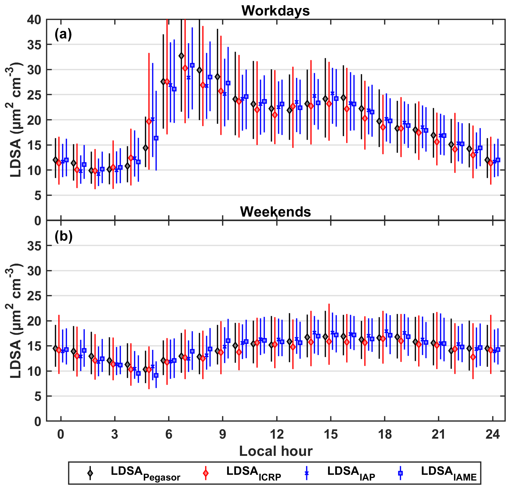
Figure 8Diurnal cycles of measured (LDSAPegasor, black), deposition-model-derived (LDSAICRP, red) and modelled (LDSAIAP and LDSAIAME, blue) LDSA concentrations with error bars of 25th and 75th percentiles on (a) workdays and (b) weekends. LDSAIAP and LDSAIAME can be differentiated by their markers, with crosses for the former and squares for the latter.
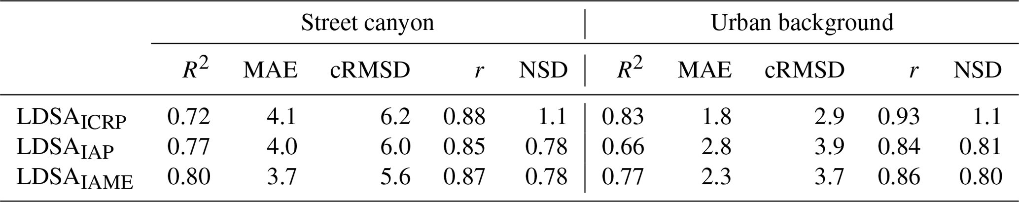
A more generalised diurnal cycle can be found in Fig. 8. The error bars of the modelled LDSAIAP and LDSAIAME were consistently smaller than those of LDSAPegasor and LDSAICRP. This might be due to the model failing to catch the extreme values, although it managed to catch the general diurnal cycle. Since outliers were removed in the pre-processing stage and the model penalised the extreme values, the model tended to give a more centralised estimate. It was a trade-off between the option with better coefficients of determination but stronger extreme errors and that with better estimations at tails but derivation of averaged estimation. This circumstance was more apparent on workdays than weekends. Furthermore, LDSAIAME could follow the diurnal cycle of LDSAPegasor much better than LDSAIAP, especially during the start of the peak hours over workdays at the SC site where the LDSA concentrations jumped to a high level. LDSAIAME can explain 80 % and 77 % of the variability of the reference measurements at SC and UB, respectively (Table 6), and compared to LDSAIAP's 77 % and 66 %, LDSAIAME performed better in terms of accuracy. In addition, the slightly smaller MAE and the proximity to 1 NSD of the LDSAIAME suggested that the mean absolute error was improved and the spread of the estimation distribution was closer to the reference measurement by taking random effects into account.
Table 6Model evaluation comparison of deposition-model-derived LDSA (LDSAICRP), modelled LDSA by IAP (LDSAIAP) and modelled LDSA by IAME (LDSAIAME) against reference measurements LDSAPegasor at the SC and UB sites. Parameters with an asterisk represent the natural logarithm. The evaluation attributes of the three methods are corrected to two significant figures.
Furthermore, we assessed the temporal and spatial impact on the IAME model by comparing the means of absolute differences between the hourly LDSAPegasor and LDSAIAME in different time windows at both stations. A descriptive statistic is presented in Table 7. We used two-sample t tests to assess whether the distributions of absolute differences were statistically significant. At SC, the p values of the t tests at all selected windows were below 0.05, which demonstrated that the performance during different seasons, days of week and hours of day of absolute differences between the measured and modelled LDSA was significantly different at the confidence level of 95 %. At the UB site, the difference between the two selected hour periods was not statistically significant. The same applied to the difference between winter and spring. There was no statistically sufficient evidence to validate the difference among the rest of the selected time period. In other words, with the use of random effects of time constraint, the overall models still performed differently at different time windows most of the time. This indicates that IAME still needs improvement in minimising temporal differences.
Table 7Statistics to show temporal difference. The number of data (n), mean and standard deviation (SD) of absolute error and the corresponding p values of t tests at the selected time windows at both sites.
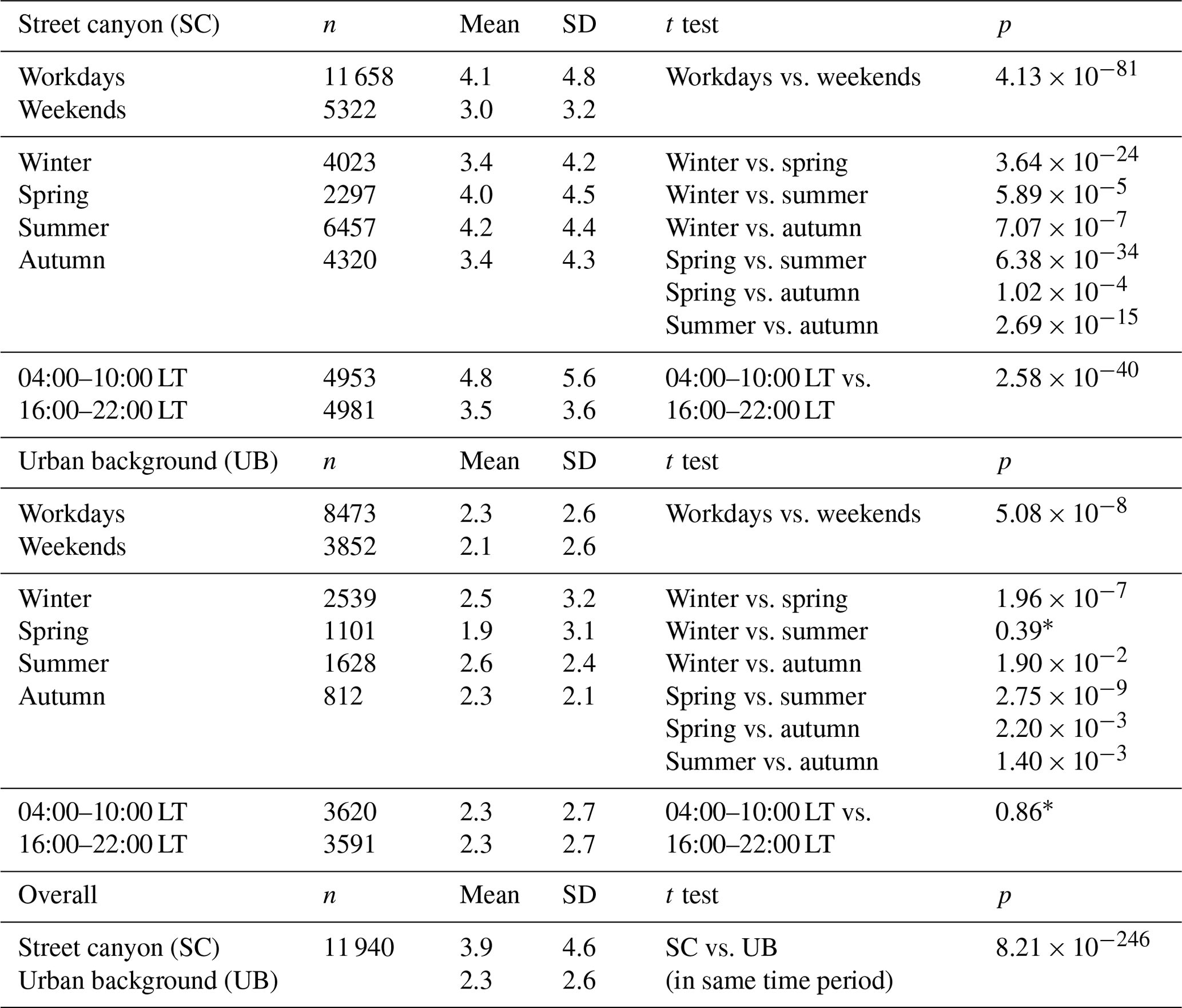
* p>0.05; the null hypothesis of different distribution is rejected.
In this study, we developed a novel input-adaptive mixed-effects (IAME) proxy to estimate alveolar LDSA by other already existing air pollutant variables and meteorological conditions in Helsinki metropolitan area. During the measurement period in 2017–2018, we retrieved LDSA measurements measured by Pegasor AQ Urban (alveolar LDSA in the ∼ 10–400 nm size range) and other variables in a street canyon (SC, average LDSA = 19.7 ± 11.3 µm2 cm−3) site and an urban background (UB, average LDSA = 11.2 ± 7.1 µm2 cm−3) site in Helsinki, Finland. Furthermore, three detached housing sites (DH, average LDSA = 11.7 ± 8.6 µm2 cm−3) and a regional background site (RB, average LDSA = 7.6 ± 5.4 µm2 cm−3) were also included as reference and background source estimation, respectively. At the SC site, LDSA concentrations were closely correlated with traffic emission. The ratio to black carbon (LDSA BC), to particle number concentration (LDSA PNC) and to nitrogen oxide (LDSA NOx) had a higher value before the morning peak and it reached its minimum during the morning peak since the role of regional background was higher for LDSA compared to those of NOx, BC and PNC. However, the ratio of LDSA to mass concentration of particles of diameter smaller than 2.5 µm (LDSA PM2.5) performed differently since the freshly emitted vehicular particles were smaller than 50 nm, which did not contribute much to PM2.5 mass concentration.
For the continuous estimation of LDSA, IAME was automatised to select the best combination of input variables, including a maximum of three fixed effect variables and three time indictors as random effect variables. Altogether, 696 submodels were generated and ranked by the coefficient of determination (R2), mean absolute error (MAE) and centred root-mean-square differences (cRMSD) in order. At the SC site, LDSA concentrations can be best estimated by PM2.5, PNC and BC, all of which were closely connected with the vehicular emissions, while they were found correlating with PM2.5, BC and carbon monoxide (CO) the best at the UB site. At both sites, PM2.5 also indicated the regionally and long-range-transported pollutants, which were a significant source of LDSA concentrations. The accuracy of the overall model was higher at the SC site (R2=0.80, MAE = 3.7 µm2 cm−3) than at the UB site (R2=0.77, MAE = 2.3 µm2 cm−3) plausibly because the LDSA source was more tightly controlled by the close-by vehicular emission source. This model could catch the temporal pattern of LDSA; however, the two-sample t tests of the residuals at all selected time windows showed that their distributions were different. This indicated that the model still performed differently at different time windows. Despite this, the novel IAME model worked better in explaining the variability of the measurements than the previously suggested IAP model as indicted by a higher R2 and lower MAE at both sites. This adjustment, by taking random effects into account, improved the sensitivity and the accuracy of the fixed effect model IAP.
The models alone cannot replace the need for reference measurements (Hagler et al., 2018). However, the IAME proxy could serve as virtual sensors to complement the measurements at reference stations in the event of missing data. The two measurement sites in this study served as a pilot of the proxy development, and the next step is to extend the work to the existing network of several measurement stations within the Helsinki metropolitan region. With similar configurations, we could fill up the voids with the information from the other stations after conscientious calibration. For example, in this paper, the two measurement sites were characterised as a street canyon and urban background. In a different setup, we may assume the similarity of the same type of environment and utilise the measurements as a replacement. Furthermore, this continuous LDSA estimation could be useful in updating some of the current air quality applications, for instance, the ENFUSER air quality model, which provides accurate spatiotemporal estimation for air pollutants in Helsinki (Johansson et al., 2015).
The air quality data and meteorological data are available from the HSY website (https://www.hsy.fi/avoindata, University of Helsinki, 2022) and through the SmartSMEAR online tool (https://smear.avaa.csc.fi/, Helsinki Region Environmental Services HSY, 2022).
The supplement related to this article is available online at: https://doi.org/10.5194/acp-22-1861-2022-supplement.
PLF performed formal analysis and writing of the original draft of the manuscript. PLF, MAZ, TP and TH conceptualised and designed the methodology of this work. MAZ, ST, MK, TP and TH provided supervision in this research activity. ES (Pegasor Oy), JVN and AKo (HSY), and HT, JK and AKa (FMI) provided instruments and data for the campaign. All the co-authors (MAZ, JVN, ES, HT, AKo, JK, TR, AKa, ST, MK, TP and TH) reviewed and commented on the manuscript.
Erkka Saukko works at Pegasor Oy, which is the manufacturer of Pegasor AQ Urban. At least one of the (co-)authors is a member of the editorial board of Atmospheric Chemistry and Physics.
Publisher’s note: Copernicus Publications remains neutral with regard to jurisdictional claims in published maps and institutional affiliations.
The authors acknowledge the City of Helsinki for providing traffic count data.
This work is supported by the European Regional Development Fund through the
Urban Innovative Action (project HOPE; Healthy Outdoor Premises for
Everyone, project no. UIA03-240) and Regional Innovations and
Experimentations Fund AIKO, governed by the Helsinki Regional Council
(project HAQT; Helsinki Air Quality Testbed, project no. AIKO014). Grants
are also received from the European Research Council through the European
Union's Horizon 2020 Research and Innovation Framework Program (grant
agreement no. 742206), and ERA-PLANET (http://www.era-planet.eu, last access: 1 February 2022) and its
transnational project SMURBS (https://www.smurbs.eu, last access: 1 February 2022) funded under the same programme
(grant agreement no. 689443). The authors wish to express their gratitude to Academy of
Finland for the funding via the Atmosphere and Climate Competence Center (ACCC) Flagship (project nos. 337549 and 337552) and NanoBioMass (project no. 1307537).
Open-access funding was provided by the Helsinki University Library.
This paper was edited by Manabu Shiraiwa and reviewed by two anonymous referees.
Albuquerque, P. C., Gomes, J. F., and Bordado, J. C.: Assessment of exposure to airborne ultrafine particles in the urban environment of Lisbon, Portugal, J. Air Waste Manage., 62, 373–380, https://doi.org/10.1080/10962247.2012.658957, 2012.
Amanatidis, S., Maricq, M. M., Ntziachristos, L., and Samaras, Z.: Application of the dual Pegasor Particle Sensor to real-time measurement of motor vehicle exhaust PM, J. Aerosol Sci., 103, 93–104, https://doi.org/10.1016/j.jaerosci.2016.10.005, 2017.
Anjilvel, S. and Asgharian, B.: A multiple-path model of particle deposition in the rat lung, Fund. Appl. Toxicol., 28, 41–50, https://doi.org/10.1006/faat.1995.1144, 1995.
Asbach, C., Fissan, H., Stahlmecke, B., Kuhlbusch, T., and Pui, D.: Conceptual limitations and extensions of lung-deposited Nanoparticle Surface Area Monitor (NSAM), J. Nanopart. Res., 11, 101–109, https://doi.org/10.1007/s11051-008-9479-8, 2009.
Asbach, C., Alexander, C., Clavaguera, S., Dahmann, D., Dozol, H., Faure, B., Fierz, M., Fontana, L., Iavicoli, I., Kaminski, H., MacCalman, L., Meyer-Plath, A., Simonow, B., van Tongeren, M., and Todea, A. M.: Review of measurement techniques and methods for assessing personal exposure to airborne nanomaterials in workplaces, Sci. Total Environ., 603, 793–806, https://doi.org/10.1016/j.scitotenv.2017.03.049, 2017.
Barreira, L. M. F., Helin, A., Aurela, M., Teinilä, K., Friman, M., Kangas, L., Niemi, J. V., Portin, H., Kousa, A., Pirjola, L., Rönkkö, T., Saarikoski, S., and Timonen, H.: In-depth characterization of submicron particulate matter inter-annual variations at a street canyon site in northern Europe, Atmos. Chem. Phys., 21, 6297–6314, https://doi.org/10.5194/acp-21-6297-2021, 2021.
Breiman, L.: Heuristics of instability and stabilization in model selection, Ann. Stat., 24, 2350–2383, https://doi.org/10.1214/aos/1032181158, 1996.
Brown, D. M., Wilson, M. R., MacNee, W., Stone, V., and Donaldson, K.: Size-dependent proinflammatory effects of ultrafine polystyrene particles: a role for surface area and oxidative stress in the enhanced activity of ultrafines, Toxicol. Appl. Pharm., 175, 191–199, https://doi.org/10.1006/taap.2001.9240, 2001.
Buonanno, G., Marini, S., Morawska, L., and Fuoco, F. C.: Individual dose and exposure of Italian children to ultrafine particles, Sci. Total Environ., 438, 271–277, https://doi.org/10.1016/j.scitotenv.2012.08.074, 2012.
Cabaneros, S. M., Calautit, J. K., and Hughes, B. R.: A review of artificial neural network models for ambient air pollution prediction, Environ. Modell. Softw., 119, 285–304, https://doi.org/10.1016/j.envsoft.2019.06.014, 2019.
Chen, J., de Hoogh, K., Gulliver, J., Hoffmann, B., Hertel, O., Ketzel, M., Bauwelinck, M., van Donkelaar, A., Hvidtfeldt, U. A., Katsouyanni, K., Janssen, N. A. H., Martin, R. V., Samoli, E., Schwartz, P. E., Stafoggia, M., Bellander, T., Strak, M., Wolf, K., Vienneau, D., Vermeulen, R., Brunekreef, B., and Hoek, G.: A comparison of linear regression, regularization, and machine learning algorithms to develop Europe-wide spatial models of fine particles and nitrogen dioxide, Environ. Int., 130, 104934, https://doi.org/10.1016/j.envint.2019.104934, 2019.
Cheristanidis, S., Grivas, G., and Chaloulakou, A.: Determination of total and lung-deposited particle surface area concentrations, in central Athens, Greece, Environ. Monit. Assess., 192, 627, https://doi.org/10.1007/s10661-020-08569-8, 2020.
Chudnovsky, A. A., Lee, H. J., Kostinski, A., Kotlov, T., and Koutrakis, P.: Prediction of daily fine particulate matter concentrations using aerosol optical depth retrievals from the Geostationary Operational Environmental Satellite (GOES), J. Air Waste Manage., 62, 1022–1031, https://doi.org/10.1080/10962247.2012.695321, 2012.
Dal Maso, M., Gao, J., Järvinen, A., Li, H., Luo, D., Janka, K., and Rönkkö, T.: Improving urban air quality measurements by a diffusion charger based electrical particle sensors-A field study in Beijing, China, Aerosol Air Qual. Res., 16, 3001–3011, https://doi.org/10.4209/aaqr.2015.09.0546, 2016.
Ding, A., Huang, X., Nie, W., Sun, J., Kerminen, V. M., Petäjä, T., Su, H., Cheng, Y., Yang, X. Q., and Wang, M.: Enhanced haze pollution by black carbon in megacities in China, Geophys. Res. Lett., 43, 2873–2879, https://doi.org/10.1002/2016GL067745, 2016.
Dockery, D. W., Pope, C. A., Xu, X., Spengler, J. D., Ware, J. H., Fay, M. E., Ferris Jr., B. G., and Speizer, F. E.: An association between air pollution and mortality in six US cities, New Engl. J. Med., 329, 1753–1759, https://doi.org/10.1056/NEJM199312093292401, 1993.
Duffin, R., Tran, C., Clouter, A., Brown, D., MacNee, W., Stone, V., and Donaldson, K.: The importance of surface area and specific reactivity in the acute pulmonary inflammatory response to particles, Ann. Occup. Hyg., 46, 242–245, https://doi.org/10.1093/annhyg/46.suppl_1.242, 2002.
Eeftens, M., Meier, R., Schindler, C., Aguilera, I., Phuleria, H., Ineichen, A., Davey, M., Ducret-Stich, R., Keidel, D., Probst-Hensch, N., Kunzli, N., and Tsai, M. Y.: Development of land use regression models for nitrogen dioxide, ultrafine particles, lung deposited surface area, and four other markers of particulate matter pollution in the Swiss SAPALDIA regions, Environ. Health, 15, 53, https://doi.org/10.1186/s12940-016-0137-9, 2016.
Faraway, J. J.: Linear models with R, edited by: Chatfield, C., Tanner, M., and Zidek, J., CRC press, ISBN 0-203-50727-4, 2014.
Fernández-Guisuraga, J. M., Castro, A., Alves, C., Calvo, A., Alonso-Blanco, E., Blanco-Alegre, C., Rocha, A., and Fraile, R.: Nitrogen oxides and ozone in Portugal: trends and ozone estimation in an urban and a rural site, Environ. Sci. Pollut. R., 23, 17171–17182, https://doi.org/10.1007/s11356-016-6888-6, 2016.
Fissan, H., Neumann, S., Trampe, A., Pui, D., and Shin, W.: Rationale and principle of an instrument measuring lung deposited nanoparticle surface area, J. Nanopart. Res., 9, 53–59, https://doi.org/10.1007/s11051-006-9156-8, 2006.
Fung, P. L., Zaidan, M. A., Sillanpaa, S., Kousa, A., Niemi, J. V., Timonen, H., Kuula, J., Saukko, E., Luoma, K., Petaja, T., Tarkoma, S., Kulmala, M., and Hussein, T.: Input-Adaptive Proxy for Black Carbon as a Virtual Sensor, Sensors (Basel), 20, 182, https://doi.org/10.3390/s20010182, 2020.
Fung, P. L., Zaidan, M. A., Surakhi, O., Tarkoma, S., Petäjä, T., and Hussein, T.: Data imputation in in situ-measured particle size distributions by means of neural networks, Atmos. Meas. Tech., 14, 5535–5554, https://doi.org/10.5194/amt-14-5535-2021, 2021a.
Fung, P. L., Zaidan, M. A., Timonen, H., Niemi, J. V., Kousa, A., Kuula, J., Luoma, K., Tarkoma, S., Petäjä, T., Kulmala, M., and Hussein, T.: Evaluation of white-box versus black-box machine learning models in estimating ambient black carbon concentration, J. Aerosol Sci., 152, 105694, https://doi.org/10.1016/j.jaerosci.2020.105694, 2021b.
Gramsch, E., Reyes, F., Oyola, P., Rubio, M., López, G., Pérez, P., and Martínez, R.: Particle size distribution and its relationship to black carbon in two urban and one rural site in Santiago de Chile, J. Air Waste Manage., 64, 785–796, https://doi.org/10.1080/10962247.2014.890141, 2014.
Gupta, R. and Xie, H.: Nanoparticles in daily life: applications, toxicity and regulations, J. Environ. Pathol. Tox., 37, 209–230, https://doi.org/10.1615/JEnvironPatholToxicolOncol.2018026009, 2018.
Habre, R., Zhou, H., Eckel, S. P., Enebish, T., Fruin, S., Bastain, T., Rappaport, E., and Gilliland, F.: Short-term effects of airport-associated ultrafine particle exposure on lung function and inflammation in adults with asthma, Environ. Int., 118, 48–59, https://doi.org/10.1016/j.envint.2018.05.031, 2018.
Hagler, G. S. W., Williams, R., Papapostolou, V., and Polidori, A.: Air Quality Sensors and Data Adjustment Algorithms: When Is It No Longer a Measurement?, Environ. Sci. Technol., 52, 5530–5531, https://doi.org/10.1021/acs.est.8b01826, 2018.
Hama, S. M. L., Ma, N., Cordell, R. L., Kos, G. P. A., Wiedensohler, A., and Monks, P. S.: Lung deposited surface area in Leicester urban background site/UK: Sources and contribution of new particle formation, Atmos. Envrion., 151, 94–107, https://doi.org/10.1016/j.atmosenv.2016.12.002, 2017.
Hastie, T., Tibshirani, R., and Tibshirani, R.: Best Subset, Forward Stepwise or Lasso? Analysis and Recommendations Based on Extensive Comparisons, Stat. Sci., 35, 579–592, https://doi.org/10.1214/19-STS733, 2020.
Helin, A., Niemi, J. V., Virkkula, A., Pirjola, L., Teinilä, K., Backman, J., Aurela, M., Saarikoski, S., Rönkkö, T., Asmi, E., and Timonen, H.: Characteristics and source apportionment of black carbon in the Helsinki metropolitan area, Finland, Atmos. Envrion., 190, 87–98, https://doi.org/10.1016/j.atmosenv.2018.07.022, 2018.
Hellén, H., Kangas, L., Kousa, A., Vestenius, M., Teinilä, K., Karppinen, A., Kukkonen, J., and Niemi, J. V.: Evaluation of the impact of wood combustion on benzo[a]pyrene (BaP) concentrations; ambient measurements and dispersion modeling in Helsinki, Finland, Atmos. Chem. Phys., 17, 3475–3487, https://doi.org/10.5194/acp-17-3475-2017, 2017.
Helsinki Region Environmental Services HSY: Open data, https://smear.avaa.csc.fi/, last access: 1 February 2022.
Hennig, F., Quass, U., Hellack, B., Kupper, M., Kuhlbusch, T. A. J., Stafoggia, M., and Hoffmann, B.: Ultrafine and Fine Particle Number and Surface Area Concentrations and Daily Cause-Specific Mortality in the Ruhr Area, Germany, 2009–2014, Environ. Health Persp., 126, 027008, https://doi.org/10.1289/EHP2054, 2018.
Hinds, W. C.: Aerosol technology: properties, behavior, and measurement of airborne particles, John Wiley & Sons, ISBN 0-471-19410-7, 1999.
Hofmann, W.: Modelling particle deposition in human lungs: modelling concepts and comparison with experimental data, Biomarkers, 14, 59–62, https://doi.org/10.1080/13547500902965120, 2009.
ICRP: PUBLICATION 66: Human Respiratory Tract Model for Radiological Protection, Pergamon Press, New York, ISSN 0146-6453, 1994.
Jafar, H. A. and Harrison, R. M.: Spatial and temporal trends in carbonaceous aerosols in the United Kingdom, Atmos. Pollut. Res., 12, 295–305, https://doi.org/10.1016/j.apr.2020.09.009, 2021.
Järvi, L., Hannuniemi, H., Hussein, T., Junninen, H., Aalto, P. P., Hillamo, R., Mäkelä, T., Keronen, P., Siivola, E., and Vesala, T.: The urban measurement station SMEAR III: Continuous monitoring of air pollution and surface–atmosphere interactions in Helsinki, Finland, Boreal Environ. Res., 19, 86–109, 2009.
Järvinen, A., Kuuluvainen, H., Niemi, J. V., Saari, S., Dal Maso, M., Pirjola, L., Hillamo, R., Janka, K., Keskinen, J., and Rönkkö, T.: Monitoring urban air quality with a diffusion charger based electrical particle sensor, Urban Clim., 14, 441–456, https://doi.org/10.1016/j.uclim.2014.10.002, 2015.
Järvinen, A., Timonen, H., Karjalainen, P., Bloss, M., Simonen, P., Saarikoski, S., Kuuluvainen, H., Kalliokoski, J., Dal Maso, M., Niemi, J. V., Keskinen, J., and Rönkkö, T.: Particle emissions of Euro VI, EEV and retrofitted EEV city buses in real traffic, Environ. Pollut., 250, 708–716, https://doi.org/10.1016/j.envpol.2019.04.033, 2019.
Johansson, L., Epitropou, V., Karatzas, K., Karppinen, A., Wanner, L., Vrochidis, S., Bassoukos, A., Kukkonen, J., and Kompatsiaris, I.: Fusion of meteorological and air quality data extracted from the web for personalized environmental information services, Environ. Modell. Softw., 64, 143–155, https://doi.org/10.1016/j.envsoft.2014.11.021, 2015.
Karjalainen, P., Timonen, H., Saukko, E., Kuuluvainen, H., Saarikoski, S., Aakko-Saksa, P., Murtonen, T., Bloss, M., Dal Maso, M., Simonen, P., Ahlberg, E., Svenningsson, B., Brune, W. H., Hillamo, R., Keskinen, J., and Rönkkö, T.: Time-resolved characterization of primary particle emissions and secondary particle formation from a modern gasoline passenger car, Atmos. Chem. Phys., 16, 8559–8570, https://doi.org/10.5194/acp-16-8559-2016, 2016.
Kiriya, M., Okuda, T., Yamazaki, H., Hatoya, K., Kaneyasu, N., Uno, I., Nishita, C., Hara, K., Hayashi, M., Funato, K., Inoue, K., Yamamoto, S., Yoshino, A., and Takami, A.: Monthly and Diurnal Variation of the Concentrations of Aerosol Surface Area in Fukuoka, Japan, Measured by Diffusion Charging Method, Atmosphere (Basel), 8, 114, https://doi.org/10.3390/atmos8070114, 2017.
Kulkarni, P., Baron, P. A., and Willeke, K. (Eds.): Aerosol measurement: principles, techniques, and applications, John Wiley & Sons, https://doi.org/10.1002/9781118001684, 2011.
Kuula, J., Kuuluvainen, H., Rönkkö, T., Niemi, J. V., Saukko, E., Portin, H., Aurela, M., Saarikoski, S., Rostedt, A., Hillamo, R., and Timonen, H.: Applicability of Optical and Diffusion Charging-Based Particulate Matter Sensors to Urban Air Quality Measurements, Aerosol Air Qual. Res., 19, 1024–1039, https://doi.org/10.4209/aaqr.2018.04.0143, 2019.
Kuula, J., Kuuluvainen, H., Niemi, J. V., Saukko, E., Portin, H., Kousa, A., Aurela, M., Rönkkö, T., and Timonen, H.: Long-term sensor measurements of lung deposited surface area of particulate matter emitted from local vehicular and residential wood combustion sources, Aerosol Sci. Tech., 54, 190–202, https://doi.org/10.1080/02786826.2019.1668909, 2020.
Kuuluvainen, H., Rönkkö, T., Järvinen, A., Saari, S., Karjalainen, P., Lähde, T., Pirjola, L., Niemi, J. V., Hillamo, R., and Keskinen, J.: Lung deposited surface area size distributions of particulate matter in different urban areas, Atmos. Envrion., 136, 105–113, https://doi.org/10.1016/j.atmosenv.2016.04.019, 2016.
Kuuluvainen, H., Poikkimaki, M., Jarvinen, A., Kuula, J., Irjala, M., Dal Maso, M., Keskinen, J., Timonen, H., Niemi, J. V., and Ronkko, T.: Vertical profiles of lung deposited surface area concentration of particulate matter measured with a drone in a street canyon, Environ. Pollut., 241, 96–105, https://doi.org/10.1016/j.envpol.2018.04.100, 2018.
Lamberg, H., Nuutinen, K., Tissari, J., Ruusunen, J., Yli-Pirilä, P., Sippula, O., Tapanainen, M., Jalava, P., Makkonen, U., Teinilä, K., Saarnio, K., Hillamo, R., Hirvonen, M.-R., and Jokiniemi, J.: Physicochemical characterization of fine particles from small-scale wood combustion, Atmos. Envrion., 45, 7635–7643, https://doi.org/10.1016/j.atmosenv.2011.02.072, 2011.
Lindstrom, M. J. and Bates, D. M.: Newton–Raphson and EM algorithms for linear mixed-effects models for repeated-measures data, J. Am. Stat. Assoc., 83, 1014–1022, https://doi.org/10.2307/2290128, 1988.
Liu, H., Zhang, X., Zhang, H., Yao, X., Zhou, M., Wang, J., He, Z., Zhang, H., Lou, L., Mao, W., Zheng, P., and Hu, B.: Effect of air pollution on the total bacteria and pathogenic bacteria in different sizes of particulate matter, Environ. Pollut., 233, 483–493, https://doi.org/10.1016/j.envpol.2017.10.070, 2018a.
Liu, Y., Wu, J., Yu, D., and Hao, R.: Understanding the patterns and drivers of air pollution on multiple time scales: the case of northern China, Environ. Manage., 61, 1048–1061, https://doi.org/10.1007/s00267-018-1026-5, 2018b.
Luoma, K., Niemi, J. V., Aurela, M., Fung, P. L., Helin, A., Hussein, T., Kangas, L., Kousa, A., Rönkkö, T., Timonen, H., Virkkula, A., and Petäjä, T.: Spatiotemporal variation and trends in equivalent black carbon in the Helsinki metropolitan area in Finland, Atmos. Chem. Phys., 21, 1173–1189, https://doi.org/10.5194/acp-21-1173-2021, 2021.
Maricq, M. M.: Monitoring Motor Vehicle PM Emissions: An Evaluation of Three Portable Low-Cost Aerosol Instruments, Aerosol Sci. Tech., 47, 564–573, https://doi.org/10.1080/02786826.2013.773394, 2013.
Mikkonen, S., Németh, Z., Varga, V., Weidinger, T., Leinonen, V., Yli-Juuti, T., and Salma, I.: Decennial time trends and diurnal patterns of particle number concentrations in a central European city between 2008 and 2018, Atmos. Chem. Phys., 20, 12247–12263, https://doi.org/10.5194/acp-20-12247-2020, 2020.
Miller, A.: Subset selection in regression, CRC Press, https://doi.org/10.1201/9781420035933, 2002.
NCRP: Report No. 125: Deposition, Retention and Dosimetry of Inhaled Radioactive Substances, National Council on Radiation Protection and Measurements, ISBN 0-929600-54-1, 1997.
Oberdörster, G.: Nanotoxicology: in vitro-in vivo dosimetry, Environ. Health Persp., 120, A13, https://doi.org/10.1289/ehp.1104320, 2012.
Oberdörster, G., Maynard, A., Donaldson, K., Castranova, V., Fitzpatrick, J., Ausman, K., Carter, J., Karn, B., Kreyling, W., Lai, D., Olin, S., Monteiro-Riviere, N., Warheit, D., Yang, H., and A report from the ILSI Research Foundation/Risk Science Institute Nanomaterial Toxicity Screening Working Group: Principles for characterizing the potential human health effects from exposure to nanomaterials: elements of a screening strategy, Part. Fibre Toxicol., 2, 1–35, https://doi.org/10.1186/1743-8977-2-8, 2005.
Pacitto, A., Stabile, L., Russo, S., and Buonanno, G.: Exposure to Submicron Particles and Estimation of the Dose Received by Children in School and Non-School Environments, Atmosphere (Basel), 11, 485, https://doi.org/10.3390/atmos11050485, 2020.
Petäjä, T., Kerminen, V.-M., Dal Maso, M., Junninen, H., Koponen, I. K., Hussein, T., Aalto, P. P., Andronopoulos, S., Robin, D., Hämeri, K., Bartzis, J. G., and Kulmala, M.: Sub-micron atmospheric aerosols in the surroundings of Marseille and Athens: physical characterization and new particle formation, Atmos. Chem. Phys., 7, 2705–2720, https://doi.org/10.5194/acp-7-2705-2007, 2007.
Pirjola, L., Niemi, J. V., Saarikoski, S., Aurela, M., Enroth, J., Carbone, S., Saarnio, K., Kuuluvainen, H., Kousa, A., Rönkkö, T., and Hillamo, R.: Physical and chemical characterization of urban winter-time aerosols by mobile measurements in Helsinki, Finland, Atmos. Environ., 158, 60–75, https://doi.org/10.1016/j.atmosenv.2017.03.028, 2017.
Reche, C., Viana, M., Brines, M., Perez, N., Beddows, D., Alastuey, A., and Querol, X.: Determinants of aerosol lung-deposited surface area variation in an urban environment, Sci. Total Environ., 517, 38–47, https://doi.org/10.1016/j.scitotenv.2015.02.049, 2015.
Rolph, G., Stein, A., and Stunder, B.: Real-time Environmental Applications and Display sYstem: READY, Environ. Model. Softw., 95, 210–228, https://doi.org/10.1016/j.envsoft.2017.06.025, 2017.
Rönkkö, T., Kuuluvainen, H., Karjalainen, P., Keskinen, J., Hillamo, R., Niemi, J. V., Pirjola, L., Timonen, H. J., Saarikoski, S., Saukko, E., Järvinen, A., Silvennoinen, H., Rostedt, A., Olin, M., Yli-Ojanperä, J., Nousiainen, P., Kousa, A., and Dal Maso, M.: Traffic is a major source of atmospheric nanocluster aerosol, P. Natl. Acad. Sci. USA, 114, 7549–7554, https://doi.org/10.1073/pnas.1700830114, 2017.
Rostedt, A., Arffman, A., Janka, K., Yli-Ojanperä, J., and Keskinen, J.: Characterization and Response Model of the PPS-M Aerosol Sensor, Aerosol Sci. Tech., 48, 1022–1030, https://doi.org/10.1080/02786826.2014.951023, 2014.
Rudin, C.: Stop explaining black box machine learning models for high stakes decisions and use interpretable models instead, Nat. Mach. Intell., 1, 206–215, https://doi.org/10.1038/s42256-019-0048-x, 2019.
Salo, L., Hyvärinen, A., Jalava, P., Teinilä, K., Hooda, R. K., Datta, A., Saarikoski, S., Lintusaari, H., Lepistö, T., Martikainen, S., Rostedt, A., Sharma, V. P., Rahman, M. H., Subudhi, S., Asmi, E., Niemi, J. V., Lihavainen, H., Lal, B., Keskinen, J., Kuuluvainen, H., Timonen, H., and Rönkkö, T.: The characteristics and size of lung-depositing particles vary significantly between high and low pollution traffic environments, Atmos. Environ., 255, 118421, https://doi.org/10.1016/j.atmosenv.2021.118421, 2021a.
Salo, L., Rönkkö, T., Saarikoski, S., Teinilä, K., Kuula, J., Alanen, J., Arffman, A., Timonen, H., and Keskinen, J.: Concentrations and Size Distributions of Particle Lung-deposited Surface Area (LDSA) in an Underground Mine, Aerosol Air Qual. Res., 21, 200660, https://doi.org/10.4209/aaqr.200660, 2021b.
Schmid, O. and Stoeger, T.: Surface area is the biologically most effective dose metric for acute nanoparticle toxicity in the lung, J. Aerosol Sci., 99, 133–143, https://doi.org/10.1016/j.jaerosci.2015.12.006, 2016.
Shiraiwa, M., Ueda, K., Pozzer, A., Lammel, G., Kampf, C. J., Fushimi, A., Enami, S., Arangio, A. M., Fröhlich-Nowoisky, J., Fujitani, Y., Furuyama, A., Lakey, P. S. J., Lelieveld, J., Lucas, K., Morino, Y., Pöschl, U., Takahama, S., Takami, A., Tong, H., Weber, B., Yoshino, A., and Sato, K.: Aerosol health effects from molecular to global scales, Environ. Sci. Technol., 51, 13545–13567, https://doi.org/10.1021/acs.est.7b04417, 2017.
Šimić, I., Lovrić, M., Godec, R., Kröll, M., and Bešlić, I.: Applying machine learning methods to better understand, model and estimate mass concentrations of traffic-related pollutants at a typical street canyon, Environ. Pollut., 263, 114587, https://doi.org/10.1016/j.envpol.2020.114587, 2020.
Taylor, K. E.: Summarizing multiple aspects of model performance in a single diagram, J. Geophys. Res.-Atmos., 106, 7183–7192, https://doi.org/10.1029/2000JD900719, 2001.
Teinilä, K., Aurela, M., Niemi, J. V., Kousa, A., Petäjä, T., Järvi, L., Hillamo, R., Kangas, L., Saarikoski, S., and Timonen, H.: Concentration variation of gaseous and particulate pollutants in the Helsinki city centre – Observations from a two-year campaign from 2013–2015, Boreal Environ. Res., 24, 115–136, 2019.
Timonen, H., Carbone, S., Aurela, M., Saarnio, K., Saarikoski, S., Ng, N. L., Canagaratna, M. R., Kulmala, M., Kerminen, V.-M., Worsnop, D. R., and Hillamo, R.: Characteristics, sources and water-solubility of ambient submicron organic aerosol in springtime in Helsinki, Finland, J. Aerosol Sci., 56, 61–77, https://doi.org/10.1016/j.jaerosci.2012.06.005, 2013.
Tissari, J.: Fine particle emissions from residential wood combustion (Puun pienpolton pienhiukkaspäästöt), Doctoral dissertation, University of Kuopio, Finland, 63 pp., ISBN 978-951-27-0975-5, 2008.
Todea, A. M., Beckmann, S., Kaminski, H., and Asbach, C.: Accuracy of electrical aerosol sensors measuring lung deposited surface area concentrations, J. Aerosol Sci., 89, 96–109, https://doi.org/10.1016/j.jaerosci.2015.07.003, 2015.
Tong, X., Ho, J. M. W., Li, Z., Lui, K.-H., Kwok, T. C., Tsoi, K. K., and Ho, K.: Prediction model for air particulate matter levels in the households of elderly individuals in Hong Kong, Sci. Total Environ., 717, 135323, https://doi.org/10.1016/j.scitotenv.2019.135323, 2020.
University of Helsinki: SmartSMEAR – About, https://www.hsy.fi/avoindata, last access: 1 February 2022.
Yeh, H.-C. and Schum, G.: Models of human lung airways and their application to inhaled particle deposition, B. Math. Biol., 42, 461–480, https://doi.org/10.1016/S0092-8240(80)80060-7, 1980.
Zaidan, M. A., Wraith, D., Boor, B. E., and Hussein, T.: Bayesian proxy modelling for estimating black carbon concentrations using white-box and black-box models, Appl. Sci., 9, 4976, https://doi.org/10.3390/app9224976, 2019.
Zaidan, M. A., Motlagh, N. H., Fung, P. L., Lu, D., Timonen, H., Kuula, J., Niemi, J. V., Tarkoma, S., Petäjä, T., Kulmala, M., and Hussein, T.: Intelligent calibration and virtual sensing for integrated low-cost air quality sensors, IEEE Sens. J., 20, 13638–13652, 2020.
Zhou, Y., Dada, L., Liu, Y., Fu, Y., Kangasluoma, J., Chan, T., Yan, C., Chu, B., Daellenbach, K. R., Bianchi, F., Kokkonen, T. V., Liu, Y., Kujansuu, J., Kerminen, V.-M., Petäjä, T., Wang, L., Jiang, J., and Kulmala, M.: Variation of size-segregated particle number concentrations in wintertime Beijing, Atmos. Chem. Phys., 20, 1201–1216, https://doi.org/10.5194/acp-20-1201-2020, 2020.