Optimizing 4 years of CO₂ biospheric fluxes from OCO-2 and in situ data in TM5: fire emissions from GFED and inferred from MOPITT CO data

Column mixing ratio of carbon dioxide (CO₂) data alone do not provide enough information for source attribution. Carbon monoxide (CO) is a product of inefficient combustion often co-emitted with CO₂. CO data can then provide a powerful constraint on fire emissions, supporting more accurate estimation of biospheric CO₂ fluxes. In this framework and using the chemistry transport model TM5, a CO inversion using Measurements of Pollution in The Troposphere (MOPITT) v8 data is performed to estimate fire emissions which are then converted into CO₂ fire emissions (called FIREMo) through the use of the emission ratio. These optimized CO₂ fire emissions are used to rebalance the CO₂ net ecosystem exchange (NEEMo) and respiration (RhMo) with the global CO₂ growth rate. Subsequently, in a second step, these rebalanced fluxes are used as priors for a CO₂ inversion to derive the NEE and ocean fluxes constrained either by the Orbiting Carbon Observatory 2 (OCO-2) v9 or by in situ (IS) CO₂ data. For comparison purpose, we also balanced the respiration using fire emissions from the Global Fire Emissions Database (GFED) version 3 (GFED3) and version 4.1s (GFED4.1s). We hence study the impact of CO fire emissions in our CO₂ inversions at global, latitudinal, and regional scales over the period 2015–2018 and compare our results to the two other similar approaches using GFED3 (FIRE3) and GFED4.1s (FIRE4) fires, as well as with an inversion using both Carnegie–Ames–Stanford Approach (CASA)-GFED3 NEE and GFED3 fire priors (priorCMS). After comparison at the different scales, the inversions are evaluated against Total Carbon Column Observing Network (TCCON) data. Comparison of the flux estimates shows that at the global scale posterior net flux estimates are more robust than the different prior flux estimates. However, at the regional scale, we can observe differences in fire emissions among the priors, resulting in differences among the NEE prior emissions. The derived NEE prior emissions are rebalanced in concert with the fires. Consequently, the differences observed in the NEE posterior emissions are a result of the balancing with fires and the constraints provided by CO₂ observations. Tropical net flux estimates from in situ inversions are highly sensitive to the prior flux assumed, of which fires are a significant component. Slightly larger net CO₂ sources are derived with posterior fire emissions using either FIRE4 or FIREMo in the OCO-2 inversion, in particular for most tropical regions during the 2015 El Niño year. Similarly, larger net CO₂ sources are also derived with posterior fire emissions in the in situ data inversion for Tropical Asia. Evaluation with CO₂ TCCON data shows lower biases with the three rebalanced priors than with the prior using CASA-GFED3. However, posteriors have average bias and scatter very close each other, making it difficult to conclude which simulation performs better than the other. We observe that the assimilated CO₂ data have a strong influence on the global net fluxes among the different inversions. Inversions using OCO-2 (or IS) data have similar emissions, mostly as a result of the observational constraints and to a lesser extent because of the fire prior used. But results in the tropical regions suggest net flux sensitivity to the fire prior for both the IS and OCO-2 inversions. Further work is needed to improve prior fluxes in tropical regions where fires are a significant component. Finally, even if the inversions using the FIREMo prior did enhance the biases over some TCCON sites, it is not the case for the majority of TCCON sites. This study consequently pushes forward the development of a CO–CO₂ joint inversion with multi-observations for a possible stronger constraint on posterior CO₂ fire and biospheric emissions.

1 Introduction

Carbon dioxide (CO₂) is the most important greenhouse gas contributing to global climate change (IPCC, 2014). Gaps in our understanding of the processes that control land–sea–atmosphere exchange of CO₂ are a leading source of uncertainty in future projections of the global climate (Friedlingstein et al., 2014). The global net flux and hence the airborne fraction can be deduced from the atmospheric growth rate (Ballantyne et al., 2012). Historically, different efforts such as the Global Carbon Project (Le Quéré et al., 2009) have divided the total global net flux into its constituent components, consisting of fluxes from the ocean, terrestrial biosphere, fossil fuel combustion and other anthropogenic activities, and biomass burning.

CO₂ emissions from fires are well characterized at the largest spatial and temporal scales, but the uncertainties increase rapidly as we look to finer spatial and temporal scales. Two approaches are currently employed to estimate global emissions from fires. The first approach uses burned-area products. The Global Fire Emissions Database (GFED) products (van der Werf et al., 2010) and the Fire INventory from NCAR (FINN) (Wiedinmyer et al., 2011), for instance, use this approach. GFED was developed for understanding the monthly contribution of fires to global carbon cycling (van der Werf et al., 2004), while FINN was developed for near-real-time estimation (Wiedinmyer et al., 2011). The second technique deduces fuel consumption from fire radiative power (FRP) determined from infrared thermal measurements. Two examples of emission inventories that use this approach are the Global Fire Assimilation System (GFAS) (Kaiser et al., 2012) and the Quick Fire Emissions Database (QFED) (Darmenov and Silva, 2015). Several studies used and compared these fire emission inventories and found several differences in capturing wildfire activity over different areas as well as sources of uncertainties from the cloud gap adjustments, small fires estimations, and land use and land cover estimation (Liu et al., 2020). While these fire emission inventories all use the MODIS thermal anomalies (Giglio et al., 2006), they use different methods of translating emission factors and land cover to estimate fire emissions. Although the quantification of emissions from biomass burning from space-based instruments has increased significantly, uncertainties regarding input data and methodologies can still lead to errors up to an order of magnitude for the total trace gas emissions (Vermote et al., 2009; Baldassarre et al., 2015).

Moving from global annual fluxes to finer scales in space and time greatly complicates the emission estimation. Interpreting atmospheric measurements of CO₂ at these scales requires the use of an atmospheric chemistry transport model (CTM) and assimilation system, frequently referred to in the literature as “atmospheric inversions” or “top-down inversions”. However, even using the same set of observations such as the Orbiting Carbon Observatory 2 (OCO-2) data in different inverse modeling systems can induce a large range of CO₂ flux estimation at regional scales (Crowell et al., 2019; Peiro et al., 2022). Flux estimates from top-down inversions have been shown to be sensitive to the choice of transport model (Schuh et al., 2019) and observational coverage (Byrne et al., 2017). Even more importantly, atmospheric measurements of CO₂ dry-air mole fractions represent the combined influence of all upstream emissions and transport, and so individual tracer measurements cannot be used to differentiate between different source or sink processes without more information. Additionally, prior estimate of the fluxes and their associated uncertainties can impact posterior CO₂ estimations (Lauvaux et al., 2012b, a; Byrne et al., 2017; Gurney et al., 2003; Wang et al., 2018; Chevallier et al., 2005; Baker et al., 2006, 2010). A few studies (Liu et al., 2017a; Palmer et al., 2019; Crowell et al., 2019; Peiro et al., 2022) utilized XCO₂ from OCO-2 to constrain top-down surface fluxes of CO₂. All of the mentioned studies found the tropics to be a large source region for 2015–2016, though the explanations varied. Crowell et al. (2019) showed that an ensemble of inversion models delivered robust results for tropical regions when OCO-2 data were assimilated. The ensemble employed included different atmospheric transport models, prior ocean and terrestrial biosphere and fire fluxes, and assimilation techniques. None of the participating models optimized fire and fossil fuel emissions. As such, only the non-fossil land (net biosphere exchange, NBE) and ocean flux at regional scales were examined in the study, with no attempt to attribute ensemble spread to different sources of uncertainty, such as the assumed fire emissions, which neglected to include some of the global inventories, such as FINN, QFED, and GFED4.1s (earlier versions of GFED were included).

Most inversion models do not explicitly constrain fire emissions with CO₂ observations. Rather, it is assumed that fire emissions have much lower uncertainty (generally believed to be less than 10 %; Le Quéré et al., 2018; Quilcaille et al., 2018) than the ocean and terrestrial biosphere fluxes (Le Quéré et al., 2018; Khatiwala et al., 2009, 2013) and so are held fixed, with the net ecosystem exchange (NEE) assumed to be the residual between the posterior total net land flux and the assumed fire and fossil fuel emissions. This assumption is problematic, not least due to the aforementioned fire emission uncertainties in time and space, which could alias into inferred biospheric fluxes at continental or regional scales (Wiedinmyer and Neff, 2007; Peylin et al., 2013). To reduce the uncertainties associated with fires and consequently with CO₂ biospheric emissions, we can examine gas species that are co-emitted with CO₂ from fires, such as carbon monoxide (CO).

CO is an air pollutant that affects the oxidation capacity of the atmosphere through its reaction with the hydroxyl radical (OH), leading to a relatively short atmospheric lifetime of 1 to 3 months because of its fast oxidation with OH. Reactions between CO and OH impact atmospheric composition on hemispheric (mainly in the tropics) or even global scales (Logan et al., 1981). CO also leads to the formation of tropospheric ozone (O₃), an important short-lived greenhouse gas, and CO₂. CO is produced by incomplete combustion, i.e., when there is not enough oxygen to make CO₂ (van der Werf et al., 2010), such as in the case of smoldering fires. In this way, CO₂ is strongly co-emitted with CO in the presence of combustion (Bakwin et al., 1997; Potosnak et al., 1999; Turnbull et al., 2006). Previous studies used trace gases such as CO to improve the CO₂ flux estimation or to separate CO₂ emission sources. Wang et al. (2010) used the CO₂ $/$ CO correlation slope to differentiate the source signature of CO₂ and separate the different characteristics of CO₂ emissions between rural and urban sites in China. Basu et al. (2014) estimated CO₂ emissions with Greenhouse gases Observing SATellite (GOSAT) data and the Comprehensive Observation Network for TRace gases by AIrLiner (CONTRAIL) project and studied seasonal variations of CO₂ fluxes during the 2009 and 2011 period over Tropical Asia. By using the Infrared Atmospheric Sounding Interferometer (IASI) CO measurements, their study showed an increased source of CO₂ in 2010 that was not caused by increased biomass burning emissions but by biosphere response to above-average temperatures. In addition to CO, some studies worked on the correlation between additional species and CO₂ to constrain CO₂ emission from biomass burning. Konovalov et al. (2014) used satellite CO and aerosol optical depth data to constrain CO₂ emissions from wildfires in Siberia by estimating FRP to biomass burning rate conversion factors. Using this approach, they found that global emission inventories underestimated CO₂ emissions from Siberia from 2007 to 2011.

As biomass burning emission estimates are necessary for constraining top-down CO₂ emissions, we want to provide our CO₂ inversion model with fire emissions that contain as much realism as possible. Fires that incorporate information from both traditional bottom-up estimation techniques and atmospheric CO data may provide a better estimate than the global inventories alone. The corresponding top-down CO₂ fluxes imposing these optimized fire emissions should have more fidelity, particularly in the tropics, where fires and the biosphere strongly interact with one another, and especially during severe drought conditions associated with the 2015–2016 El Niño. The objective of this paper is to assess the improvement in CO₂ biogenic emission estimates when CO-informed fire emissions are imposed, particularly during the 2015–2016 El Niño event and the subsequent years (2017 and 2018). First, we constrain CO emissions using data from the Measurements of Pollution in The Troposphere (MOPITT). We use these optimized CO emissions together with key vegetation parameters from GFED to create an updated estimate of fire CO₂ emissions that incorporates both sets of information. Finally, these updated fire emissions and appropriately rebalanced prior biogenic fluxes are imposed in an atmospheric CO₂ inversion to constrain the net land and ocean CO₂ fluxes using either OCO-2 XCO₂ retrievals or in situ data. To evaluate these new emissions, an alternative set of fire emissions and rebalanced prior biogenic fluxes have also been used in this CO₂ inversion framework.

This paper is ordered as follows. The assimilation and evaluation data sets and the inversion modeling framework are described in Sect. 2. The results for CO and CO₂ flux estimates and evaluation against independent data are presented in Sect. 3. The importance of these inversion results are discussed in Sect. 4. Conclusions and proposed future work are presented in Sect. 5. Description of the different GFED versions are presented in Appendix A.

2 Data and methodology

Our experiments focus on estimation of top-down fluxes using the TM5–4D-Var system (e.g., Meirink et al., 2008; Basu et al., 2013; Crowell et al., 2018). Our inversions are performed in sequence: (1) we assimilate total column CO retrievals from the MOPITT v8 products to produce optimized CO fluxes, which are used to update the assumed CO₂ fire emissions, and then (2) we assimilate either total column CO₂ from OCO-2 version 9 retrievals or CO₂ in situ data to produce optimized CO₂ NEE and ocean fluxes. We introduce hereafter the observations used in the inversions, the inversion system, and the observations used for validation.

2.1 Data sets

2.1.1 MOPITT data

Space-based CO data are available from a large variety of instruments: IASI (Infrared Atmospheric Sounding Interferometer, Turquety et al., 2004; Clerbaux et al., 2009) aboard the Metop satellite, MOPITT (Measurements of Pollution in the Troposphere, Drummond et al., 2010, 2016) aboard the Terra satellite, the Tropospheric Emission Spectrometer (TES, Beer et al., 2001) aboard EOS-Aura and the Atmospheric InfraRed Sounder (AIRS, Aumann et al., 2003) aboard EOS-Aqua. These satellite data can be used to monitor fire emissions from an atmospheric point of view. So far, MOPITT has been the only space-based instrument deriving CO from near-infrared (NIR), thermal infrared (TIR), and multispectral radiances (TIR + NIR). Recently, the TROPOspheric Monitoring Instrument (TROPOMI, Landgraf et al., 2016) and GOSAT-2 TANSO-FTS-2 (http://www.gosat-2.nies.go.jp/, last access: 12 December 2022) are also retrieving CO from NIR radiances. However, MOPITT products have been consistently validated against airborne vertical profiles and ground-based measurements, allowing a well-understood product (Worden et al., 2010; Deeter et al., 2019).

MOPITT (Drummond, 1993) was launched in 1999 on board the Terra satellite. Terra flies in a sun-synchronous polar orbit at an altitude of 705 km, crossing the Equator at approximately 10:30 LT (local time) each morning and evening. It has a nadir view with spatial resolution of 22×22 km. Its swath is 650 km wide, with 116 cross-track footprints. MOPITT achieves a global coverage in about 4 d.

MOPITT uses gas filter correlation radiometry to retrieve CO mixing ratios from radiances in the 4.7 µm (TIR) and 2.3 µm (NIR) spectral bands. TIR-only retrievals of MOPITT have been shown to be mostly sensitive to CO in the mid-upper troposphere (excluding regions with strong thermal gradients such as deserts, Deeter et al., 2007). NIR-only retrievals depend on reflected solar radiation and are also used for retrievals of CO total column, though the vertical sensitivity is stronger near the surface than the TIR-only retrievals (Deeter et al., 2009; Worden et al., 2010). MOPITT TIR + NIR retrievals can provide improved estimates of CO near source locations and have enhanced land surface sensitivity compared to the TIR-only product (Deeter et al., 2015). In this study, we consequently use the level 2 TIR–NIR profiles product in order to have better sensitivity of CO on the total column with greatest sensitivity in the lower troposphere (Deeter et al., 2013). With the observing limitations of NIR data, this product is limited to daytime observations over land. In addition, because retrievals with surface pressures less than 900 hPa might be of lower quality, they are removed for the assimilation (Fortems-Cheiney et al., 2011; Yin et al., 2015). MOPITT retrieval products are generated with an optimal estimation-based retrieval algorithm and a fast radiative transfer model involving both MOPITT calibrated radiances and a priori knowledge of CO variability (Deeter et al., 2003). The MOPITT operational fast forward model (MOPFAS) is a radiative transfer model based on the HITRAN2012 (Rothman et al., 2013) database with CO parameters in log(VMR) used to simulate the MOPITT measured radiances (Edwards et al., 1999). For this retrieval method, cloud-free observations are required. The MOPITT v8 products consist of CO profile with 10 pressure levels. In our assimilation system, simulated values of logXCO using the MOPITT v8 averaging kernel are compared to the retrievals, and the difference is then propagated into flux adjustments using the TM5 adjoint.

Several studies have used inverse modeling with MOPITT data to estimate CO emissions (Huijnen et al., 2016; Yin et al., 2016; Nechita-Banda et al., 2018), and they showed that MOPITT v7 data have poor performance at detecting extreme events. However, MOPITT v8 implemented a bias correction in the radiance which demonstrated improved retrievals relative to v7 (Deeter et al., 2019). In particular, MOPITT v8 does not exhibit a latitudinal dependence in partial CO column biases observed in v7 (Deeter et al., 2019). MOPITT v8 TIR–NIR product biases are within 5 % at all levels when compared to NOAA aircraft profiles. In addition, apparent long-term trends in v7 biases have been decreased to 0.1 % yr⁻¹ or less at all retrieval levels for v8 products (Deeter et al., 2019). We thus expect to have better performance in the detection of extreme events by assimilating MOPITT v8 and less bias in the inferred CO emissions overall.

2.1.2 OCO-2 data

The OCO-2 (Crisp et al., 2017; Eldering et al., 2017) satellite was launched in July 2014 as the first NASA mission dedicated to observing CO₂ from space. The satellite flies in a sun-synchronous orbit with an altitude of 705 km and a 16 d revisit time. OCO-2 passes each location at approximately 13:30 LT (Crisp and Johnson, 2005). OCO-2 observes eight footprints across a 10 km ground track, each of which is less than 1.29 km by 2.25 km (Eldering et al., 2017). Smaller spatial footprints increase the number of cloud-free scenes, allowing for more successful retrievals with lower errors (O'Dell et al., 2018), e.g., relative to the Greenhouse gases Observing SATellite (GOSAT; Kuze et al., 2009).

OCO-2 measures the absorption of solar reflectance spectra within CO₂ (1.6 and 2.0 µm) and molecular oxygen (O₂) bands (0.76 µm). Retrievals from OCO-2 have sensitivity throughout the entire troposphere with the highest sensitivity close to the surface (Eldering et al., 2017). As with CO, retrievals of CO₂ from TIR observations such as those from TES or AIRS typically have lower sensitivity in the atmospheric boundary layer (Eldering et al., 2017).

CO₂ retrieval products come from the Atmospheric Carbon Observations from Space (ACOS) retrieval algorithm (O'Dell et al., 2012; Crisp et al., 2012; O'Dell et al., 2018; Kiel et al., 2019). OCO-2 radiance measurements are analyzed with remote sensing retrieval algorithms to spatially estimate column-averaged CO₂ dry-air mole fraction, XCO₂. This quantity represents the average concentration of CO₂ in a column of dry air from the surface to the top of the atmosphere. ACOS XCO₂ product have been largely validated against ground-based observations from the Total Carbon Column Observing Network (TCCON; Wunch et al., 2017). Our study uses the OCO-2 version 9 data product, as it contains all of the improvements as well as a bug fix that was found after the release of version 8 (v8). Being a nonlinear optimal estimation product, retrievals contain residual errors that must be removed through the use of a bias correction (O'Dell et al., 2018; Kiel et al., 2019). Residual biases in XCO₂ were reduced especially over rough topography and were found to be caused by relative pointing offsets between the three bands. Even after the bias correction is applied, errors on regional scales likely remain (O'Dell et al., 2018). Despite these shortcomings, data coverage from satellites is dense in the tropics relative to the global in situ network, which has very few sites there. Despite the known shortcomings (biases) of satellite data, several studies have preferred to use satellite data over the tropics to take full advantage of the improved spatial coverage. For instance, Liu et al. (2017a) and Palmer et al. (2019) have discussed the impacts of the 2015–2016 El Niño event on the carbon cycle, particularly in the tropics using OCO-2 v7. In addition, OCO-2 retrievals have been used in several inversion models. For example, Crowell et al. (2019) showed that with different assumptions (such as a large ensemble of atmospheric inversions using different CTM, data assimilation algorithms, and prior flux), OCO-2 posterior inferred fluxes globally agree with in situ data, but that this agreement breaks down quickly at smaller spatial and temporal scales.

To finish regarding the data we are using in our study, Huijnen et al. (2016) and Patra et al. (2017) have shown that pyrogenic CO₂ emission estimates from CO MOPITT data (through the use of emission factors) are consistent with OCO-2 measurements using a forward simulation with a CTM. With this in mind and also that OCO-2 and MOPITT have similar vertical sensitivity for their retrievals of CO₂ and CO, we use these two data sets to constrain surface fluxes for these two tracers. Using CO₂ and CO together in this way is an important proof of concept for upcoming missions such as GeoCarb (Moore et al., 2018), which will measure both tracers from geostationary orbit over the Americas.

2.1.3 In situ data

The in situ CO₂ data used for assimilation come from five collections in ObsPack format (Masarie et al., 2014). These collections include

• the obspack_co2_1_GLOBALVIEWplus_v5.0_2019-08-12 (Cooperative Global Atmospheric Data Integration Project, 2019), which contributes to 93 % of all data;

• obspack_co2_1_NRT_v5.0_2019-08-13 (NOAA Carbon Cycle Group ObsPack Team, 2019), which provides near-real-time provisional observation, and so the data did not get final quality control;

• obspack_co2_1_AirCore_v2.0_2018-11-13, which is provided by the balloon-borne AirCore instrument; this data set includes almost the entire atmospheric column;

• obspack_co2_1_INPE_RESTRICTED_v2.0_2018-11-13 (NOAA Carbon Cycle Group ObsPack Team, 2018); this collection of data only comes from aircraft profiles at fives sites in Brazil;

• obspack_co2_1_NIES_Shipboard_v2.1_2019-06-12; the data come from nine volunteer ships of opportunity operated by the Japanese National Institute for Environmental Studies (Tohjima et al., 2005; Nara et al., 2017).

These five collections provide around 540 assimilable observations per day. These CO₂ measurements are collected in flasks or by continuous analyzers at surface, tower, and aircraft sites (see Fig. S1 in the Supplement) and are an important anchor for this exercise because their error characteristics are generally well known, being directly established via calibration traceable to World Meteorological Organization standards. Additionally, these measurements provide traceability to a long history of flux estimates derived from these data as an atmospheric constraint.

2.1.4 Observations for validation: TCCON data

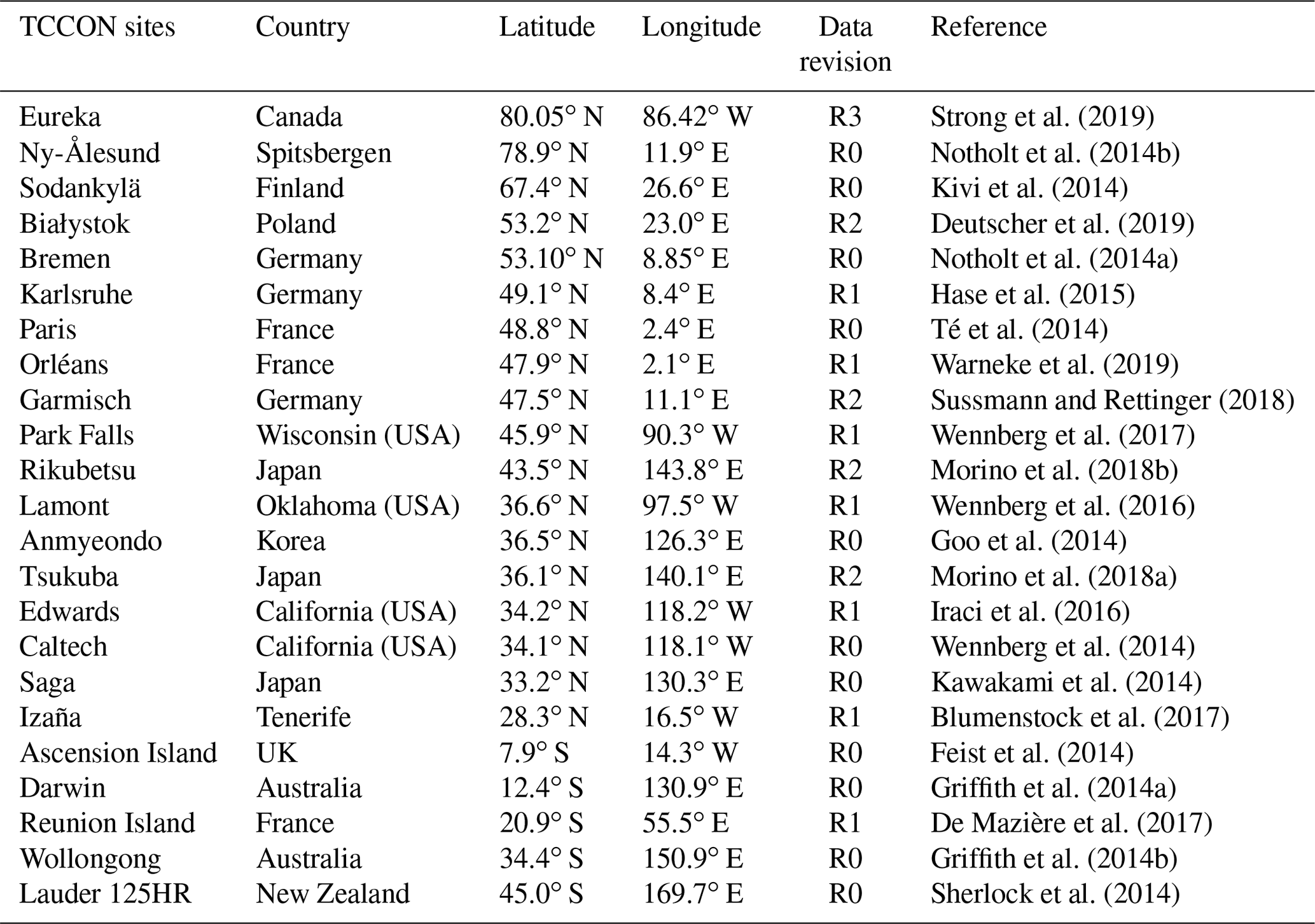
We evaluate our posterior model mole fractions against retrievals from TCCON, which is a ground-based network of Fourier transform spectrometers established in 2004 and designed to retrieve atmospheric gases from NIR spectra (Wunch et al., 2011). The global monthly means of the total column CO₂ measurements have accuracy and precision better than 0.25 % (less than 1 ppm) relative to validation with aircraft measurements (Wunch et al., 2010, 2011). TCCON measurements have been used in several papers for validation of satellite measurements (e.g., Kulawik et al., 2016; Wunch et al., 2017; O'Dell et al., 2018; Kiel et al., 2019). Our evaluation uses data from 23 operational instruments of TCCON globally. Table 1 lists all TCCON sites used for the evaluation, and Fig. S2 shows the site locations over the globe.

Strong et al. (2019)Notholt et al. (2014b)Kivi et al. (2014)Deutscher et al. (2019)Notholt et al. (2014a)Hase et al. (2015)Té et al. (2014)Warneke et al. (2019)Sussmann and Rettinger (2018)Wennberg et al. (2017)Morino et al. (2018b)Wennberg et al. (2016)Goo et al. (2014)Morino et al. (2018a)Iraci et al. (2016)Wennberg et al. (2014)Kawakami et al. (2014)Blumenstock et al. (2017)Feist et al. (2014)Griffith et al. (2014a)De Mazière et al. (2017)Griffith et al. (2014b)Sherlock et al. (2014)

Table 1 Geolocation and reference of each TCCON station used for the evaluation section.

2.2 Chemistry transport model TM5

We employ TM5 (Krol et al., 2005) and the four-dimensional variational (4D-Var, Meirink et al., 2008) framework to link trace gas emissions to atmospheric tracer mixing ratios. Several inverse modeling studies have estimated CO emissions or CO₂ emissions using TM5–4D-Var (Hooghiemstra et al., 2011; Van Leeuwen et al., 2013; van der Laan-Luijkx et al., 2015; Nechita-Banda et al., 2018; Basu et al., 2018; Crowell et al., 2018, 2019). TM5 is driven by 3-hourly offline meteorological fields from the ERA-Interim (Dee et al., 2011) reanalysis of the European Centre for Medium-Range Weather Forecasts (ECMWF). We run TM5 on a $\mathrm{3}{}^{\circ }\times \mathrm{2}{}^{\circ }$ horizontal resolution grid for the CO inversion and on a $\mathrm{6}{}^{\circ }\times \mathrm{4}{}^{\circ }$ horizontal resolution grid for the CO₂ inversions with 25 vertical hybrid sigma-pressure levels. The initial condition for CO is globally constant to 80 ppb, which is then combined with a 6-month spin-up to account for discrepancies from the real atmospheric distribution of CO. The initial global distribution of CO₂ is taken from the CarbonTracker (Peters et al., 2007 version CT2017, with updates documented at http://carbontracker.noaa.gov, last access: 12 December 2022) posterior mole fractions. The CT2017 fields are constrained over the period 2000–2016 with data from the global in situ network. Both inversions are run from 1 July 2014 until 1 March 2019, i.e., with 6 months of spin-up and 2 months of spin-down to avoid so-called “edge effects””affecting the period of interest from 2015–2018.

The CO sink from OH is represented in TM5 by a monthly OH climatology from Spivakovsky et al. (2000). This OH climatology is scaled by a factor 0.92 based on methyl chloroform simulations (Huijnen et al., 2010).

2.3 Inversion system and analyses

We use TM5–4D-Var to infer fluxes as the long window ensures a long-term spatiotemporal distribution of the trace gas in the atmosphere that is consistent with multi-year flux distributions. The TM5–4D-Var model is used in this study to estimate CO and CO₂ emissions with the corresponding satellite and in situ. TM5–4D-Var utilizes optimal estimation to minimize a Bayesian cost function (Rodgers, 2000) in order to find the state vector corresponding to surface emissions of CO or CO₂ that best match the observations within their relative uncertainties. The a posteriori flux is found by minimizing the mismatch between the forward model and the observations weighted by the inverse of the observation error covariance matrix R while staying close to a set of a priori fluxes weighted by the inverse of the a priori error covariance matrix B. These matrices are discussed in more detail in Sect. 2.3.1. If TM5 cannot represent the synoptic variability accurately, then the resulting errors when comparing the model with observations will prevent these observations from being used effectively in the 4D-Var. The mismatch between the model and the observation due to the differences in the resolution of the tracer transport model (including both the resolution of the meteorological ERA-Interim fields and the resolution of the fluxes on the model grid) and the resolution of the observation footprint is also known as the representativeness error (observational error). If the observational error in data assimilation is not correctly accounted for, there will be errors in the optimized parameters (surface fluxes). For more information on the calculation of observational error in TM5, see Bergamaschi et al. (2010). However, it has been shown in previous studies that going from coarse resolution of the global tracer transport models to higher resolution does not provide improvement with respect to observations (Lin et al., 2018; Remaud et al., 2018).

Fluxes and measured concentrations are linked through the transport and the observation operator. The observations are not aggregated at the model resolution. Although the CTM is quasi-linear, the observation operator for CO is not. Since we use log(VMR) for the MOPITT retrievals as the CO observable, the nonlinear optimizer M1QN3 from Gilbert and Lemaréchal (1989) is employed. Both the transport and observation operators for CO₂ are linear, and so we employ the conjugate gradient method to estimate the optimal CO₂ emissions, the implementation of which is described in great detail in Basu et al. (2013). Due to some information gaps in the observational coverage, there is not enough information for the state vector. Therefore, the prior fluxes are used as the foundation to which we make corrections with information from the observations. These corrections are determined by the prior uncertainty and the model–data mismatch statistics.

2.3.1 A priori information

(a) CO parameterizations

Injection heights, in the CO inversion, are computed using IS4FIRES (Integrated System for Wild-Land Fires, http://is4fires.fmi.fi/, last access: 12 December 2022, Sofiev et al., 2013). This emission database is driven by reanalysis FRP obtained from the MODIS (Giglio et al., 2006) instrument on board Aqua and Terra satellites.

Three emission categories are used for the CO inversion: anthropogenic (which represents the combustion of fossil fuels and biofuels), natural sources (direct CO emissions from vegetation and oceans), and biomass burning (vegetation fires). In our configuration, we only optimize biomass burning emissions.

Anthropogenic emissions come from the MACCity inventory (Granier et al., 2011). This inventory provides projected inter-annual trends in the anthropogenic CO emissions.

The oxidation of CH₄ and non-methane volatile organic compounds (NMVOCs) such as isoprene (C₅H₈) and monoterpene (C₁₀H₁₆) leads through photolysis and reaction with OH to the formation of formaldehyde, the major chemical source of CO (Atkinson, 2000). Isoprene is a member of the group of hydrocarbons known as terpenes. It is explicitly taken into account in TM5 as it represents the dominant biogenic NMVOC emission (Guenther et al., 2012). Isoprene and monoterpene oxidation schemes are based on the mechanisms developed by Yarwood et al. (2005). Isoprene contributes to 9 %–16 % of the global CO burden (Pfister et al., 2008). They account for 68 % in TM5 of the biogenic NMVOC emissions that react to produce CO. By contrast, monoterpene accounts for 15 % (Tsigaridis et al., 2014). The chemical production of CO coming from the oxidation of methane and NMVOCs requires monthly 3-D CO fields produced by oxidation of biogenic and anthropogenic hydrocarbons including CH₄. We use chemical production of CO from the oxidation of CH₄ and from NMVOCs by using a 2010 simulation with the full chemistry version of TM5 (Huijnen et al., 2010).

A priori biomass burning CO emissions are taken from the GFED4.1s inventory (van der Werf et al., 2010) and incorporate a daily cycle. Further description of the GFED versions can be found in Appendix A. GFED4.1s has a spatial resolution of $\mathrm{0.25}{}^{\circ }\times \mathrm{0.25}{}^{\circ }$ and includes estimates of burned area, carbon emissions, monthly biospheric carbon fluxes based on the Carnegie–Ames–Stanford Approach (CASA)-GFED4s framework, and the information from the small-fire fraction. Additionally, monthly carbon emissions of GFED4.1s distinguish between different vegetation types such as boreal forest, agricultural waste, temperate forest, deforestation, peatland, and savanna.

The prior uncertainty covariance matrix B is described by a product of uncertainty variance and correlations in space and time. Spatially, a Gaussian correlation length scale of 1000 km is used, as justified in Meirink et al. (2008), while we assume the prior errors have a temporal correlation scale of 4 d. As in Hooghiemstra et al. (2011, 2012) and Nechita-Banda et al. (2018), an uncertainty standard deviation of 250 % has been applied for the grid-scale prior of biomass burning emission. This large uncertainty is assumed since these inventories support large uncertainties. As mentioned by Hooghiemstra et al. (2011), this yields between 40 %–100 % of prior continental emission uncertainty, depending on the region. The observation covariance matrix R includes two errors: instrument errors and transport model errors. In this matrix R, we only assume uncorrelated errors, meaning we only have errors along the diagonal. This can be assumed since observation error is in general easily quantifiable by careful calibration of instruments.

(b) Computation of an optimized CO₂ fire prior

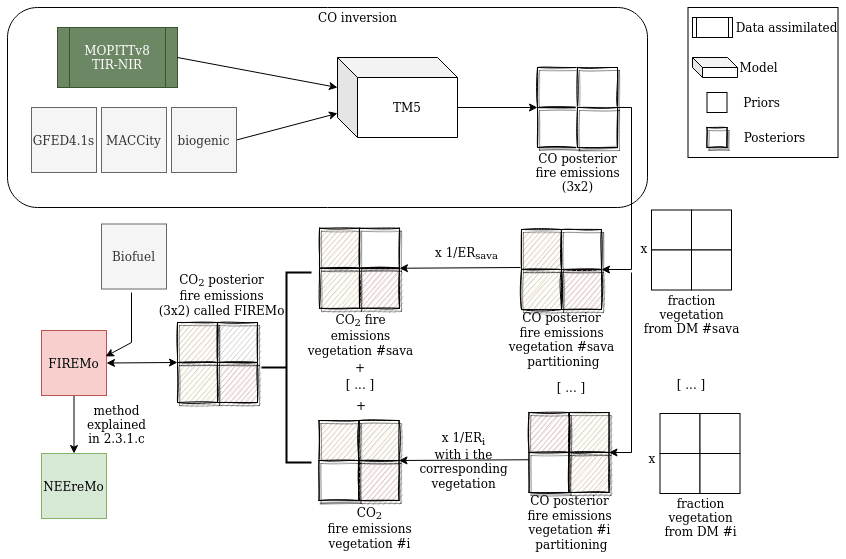
In this section, we describe the computation of our optimized prior fire emission (FIREMo), which we use to observe the impact of CO fire emissions in posterior CO₂ biospheric fluxes. The steps of FIREMo calculation are shown in Fig. 1. For each pixel ($\mathrm{3}{}^{\circ }\times \mathrm{2}{}^{\circ }$ resolution) of CO posterior fire emissions, we applied a vegetation fraction based on the dry matter product (DM) of GFED4.1s. We obtained fire emissions for each monthly vegetation type (savanna, boreal forests, peat, temperate forests, deforestation, and agriculture waste). Figure S3 shows GFED DM vegetation type for each year over land, where each pixel represents one or more vegetation types.

Figure 1 Flowchart of the FIREMo calculation.

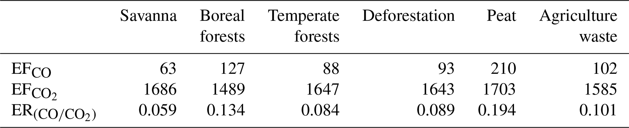
We first calculated the emission ratios ER${}_{\left(\mathrm{CO}/{\mathrm{CO}}_{\mathrm{2}}\right)}$, which allowed us to convert CO fire emissions to CO₂ fire emissions. The emission ratios are computed using GFED emission factor for each vegetation type (annotated i in the Eq. 1). Following the equation of Andreae and Merlet (2001):

$$\begin{array}{}\text{(1)}& {\mathrm{ER}}_{{\left(\mathrm{CO}/{\mathrm{CO}}_{\mathrm{2}}\right)}_i}={\displaystyle \frac{{\mathrm{EF}}_{{\mathrm{CO}}_i}}{{\mathrm{EF}}_{{{\mathrm{CO}}_{\mathrm{2}}}_i}}}\cdot {\displaystyle \frac{M_{{\mathrm{CO}}_{\mathrm{2}}}}{M_{\mathrm{CO}}}},\end{array}$$

with M_CO=28 g mol⁻¹ and $M_{{\mathrm{CO}}_{\mathrm{2}}}=\mathrm{44}$ g mol⁻¹ the molecular weights of CO and CO₂; EF represents the emission factors for each vegetation type described in Table 2. Emission factors allow us to estimate trace gas emissions from carbon losses during fires (Andreae and Merlet, 2001). For better comparison we applied the same emission factors used by the OCOCMS product (based on Andreae and Merlet, 2001, and Akagi et al., 2011) and not the more recent emission factors provided by Andreae (2019).

Table 2 Emission factors (in grams per kilogram of dry matter burned) for CO and CO₂, and emission ratios ER${}_{\left(\mathrm{CO}/{\mathrm{CO}}_{\mathrm{2}}\right)}$ available from GFED4.1s by vegetation types based on van der Werf et al. (2017).

We then aggregated the $\mathrm{0.25}{}^{\circ }\times \mathrm{0.25}{}^{\circ }$ vegetation fraction partitioning of GFED to create the vegetation fraction product at a $\mathrm{3}{}^{\circ }\times \mathrm{2}{}^{\circ }$ grid (see Fig. 1). We applied this aggregated fraction to the posterior simulated CO fires, which partitioned the posterior CO fires by vegetation types. Finally, the emission ratio for each vegetation type was divided into the posterior CO fire partitioned for each vegetation type (Basu et al., 2014). This results in monthly CO₂ emission per vegetation type at a $\mathrm{3}{}^{\circ }\times \mathrm{2}{}^{\circ }$ resolution. Finally, we sum up these emissions across all surface types and also include CO₂ biofuel emissions (see Table 3) in order to get monthly total optimized prior CO₂ biomass burning emissions that we called “FIREMo” (see Fig. 1). We used FIREMo as fire prior emissions in CO₂ inversions along with a rebalanced respiration and NEE (in balance with fire estimate), using the parameterization described in “(c) CO₂ parameterizations”.

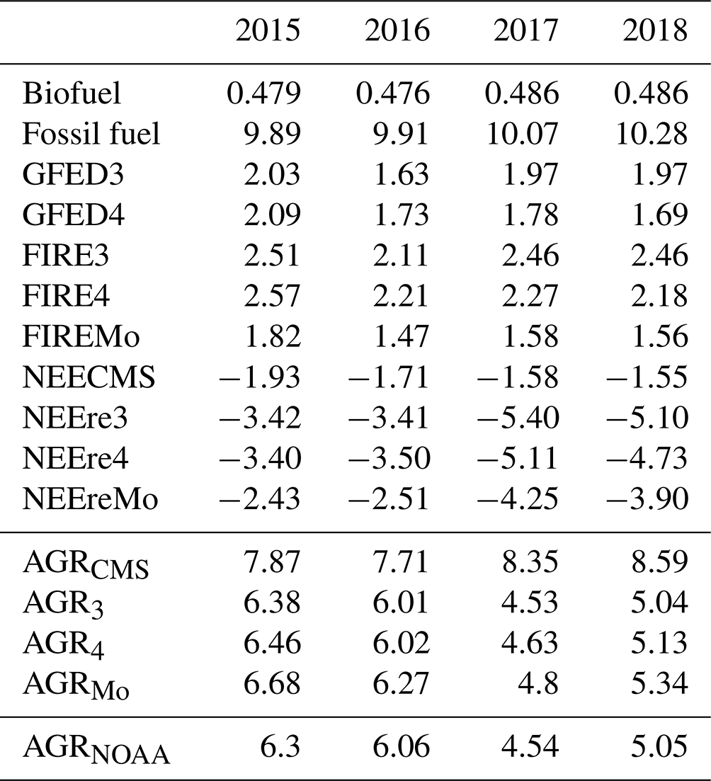
Table 3 Global total fossil fuel emissions, fire from GFED3 and GFED4.1s, FIRE (fire + biofuel), biofuel emissions, and AGR from NOAA in Pg C yr⁻¹.

(c) CO₂ parameterizations

CO₂ emissions are separated into four categories: anthropogenic sources, ocean fluxes, terrestrial biosphere fluxes (meaning the sum of the photosynthesis and respiration), and fires.

The anthropogenic emissions are taken from the Open-source Data Inventory for Anthropogenic CO₂ 2018 (ODIAC2018; Oda and Maksyutov, 2011). A diurnal cycle is imposed by the Temporal Improvements for Modeling Emissions by Scaling (TIMES) product with weekly scaling as suggested by Nassar et al. (2013). Fossil fuel emissions are not optimized in the CO₂ inversions, as is typical of global tracer transport inversions (e.g., Peylin et al., 2013; Crowell et al., 2019). Ocean fluxes are taken from Takahashi et al. (2009). They are assumed to have an uncertainty variance of 50 %. Both biospheric and oceanic emissions are optimized in the CO₂ inversions. The uncertainties in the prior fluxes are derived from different climatological fluxes with exponential spatiotemporal correlation assumed. For the oceanic component, the horizontal correlation is 1000 km and the timescales is 3 weeks, while for the terrestrial component, the length and timescale are 250 km and 1 week. These uncertainties are applied similarly to all experiments.

Terrestrial biosphere fluxes and fire emissions are difficult to disentangle from CO₂ data alone, and some inverse modeling studies (e.g., Crowell et al., 2019) choose instead to report the net land fluxes. Likewise, some global land flux estimates such as the GEOS-Carb CASA-GFED3 project (Ott, 2020) use fire estimates with ecosystem respiration to revise the terrestrial biosphere flux estimates. We take a similar (but not identical) approach, using emissions of fire and respiration to estimate the terrestrial biosphere flux. We start with the gross primary production and respiration estimates from the CASA-GFED3 3-hourly $\mathrm{0.5}{}^{\circ }\times \mathrm{0.625}{}^{\circ }$ resolution (Ott, 2020). We then modify the net flux in concert with each fire emission estimated as follows.

Net ecosystem exchange (NEE) in the CASA-GFED3 product is expressed as the sum of heterotrophic respiration (Rh) and gross ecosystem exchange (GEE):

$$\begin{array}{}\text{(2)}& \mathrm{NEE}\mathrm{3}=\mathrm{Rh}\mathrm{3}+\mathrm{GEE}\mathrm{3}.\end{array}$$

We modified the respiration from CASA-GFED3 (Rh3, respiration linked to FIRE3) to create respiration estimates for GFED4.1s (Rh4, respiration linked to FIRE4) and FIREMo (RhMo, respiration in balance with the updated CO₂ fire estimate FIREMo), so that estimated respiration increases (decreases) in the places where each fire estimate is smaller (larger) than FIRE3 (GFED3):

$$\begin{array}{}\text{(3)}& \mathrm{Rh}x=\mathrm{Rh}\mathrm{3}+\max (\mathrm{FIRE}\mathrm{3}-\mathrm{FIRE}x,\mathrm{0}),\end{array}$$

where x is either “4” or “Mo”. This equation means that the difference between FIRE3 and FIREx is cut off at 0 when the difference is negative. With this equation we only consider the positive difference (when we have lower FIREx emissions than FIRE3). The resulting net ecosystem exchange, i.e., NEE4 or NEEMo, is then computed using Eq. (2), with GEE3 used for both NEE4 or NEEMo equations. We then apply a simple rebalancing scheme to match the yearly NOAA global mean growth rate (AGR_NOAA) for 2015–2018 (see Table 3), since

$$\begin{array}{}\text{(4)}& \mathrm{AGR}=\stackrel{\mathrm{‾}}{\mathrm{NEE}}+\stackrel{\mathrm{‾}}{\mathrm{fire}}+\stackrel{\mathrm{‾}}{\mathrm{fossil}}+\stackrel{\mathrm{‾}}{\mathrm{biofuel}}+\stackrel{\mathrm{‾}}{\mathrm{ocean}},\end{array}$$

where $\stackrel{\mathrm{‾}}{X}$ represents the global total annual flux for category X. We use ODIACv2018 (with 2018 repeated for 2019) to compute the global fossil fuel totals (values in the Table 3), biofuel from the CASA land biosphere model (van der Werf et al., 2004), and a fixed annual value of −2.6 Pg C yr⁻¹ for the oceans for simplicity, and we use FIRE from each source described above.

Any mismatch between the AGR derived from our prior flux estimates (AGR_x) and AGR_NOAA is assumed to be due to an incorrect estimate of global NEE. We adjust NEE at each grid point with a simple scaling on global total respiration (i.e., Rhx) and GEE:

$$\begin{array}{}\text{(5)}& {\mathrm{AGR}}_{\mathrm{NOAA}}-{\mathrm{AGR}}_x=(\mathrm{1}+k)\stackrel{\mathrm{‾}}{\mathrm{Rh}x}+(\mathrm{1}-k)\stackrel{\mathrm{‾}}{\mathrm{GEE}},\end{array}$$

where x is either 3, 4, or Mo, depending on whether we use FIRE3 (GFED3), FIRE4 (GFED4.1s), or FIREMo. This equation is easily solved for k using each annual global total, and the resulting corrections are applied to each 3-hourly gridded value of GEE and respiration for each choice of fire emissions. In this way, the a priori global CO₂ emissions are ensured to match the annual global growth rate as measured by NOAA regardless of the fire emissions assumed, as well as a spatial pattern and seasonality that aligns with bottom-up models' GEE and Rh estimates as closely as possible.

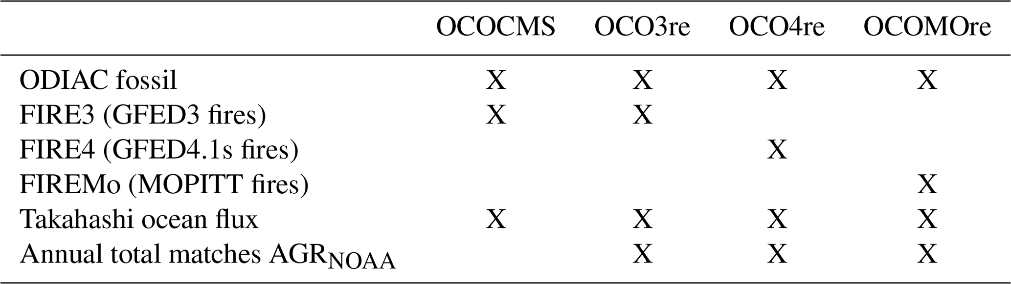
We run the CO₂ inversions with the rebalanced terrestrial biosphere net flux NEErex corresponding to either FIRE3, FIRE4, or FIREMo priors. In order to assess the impacts of the rebalancing procedure, we perform a fourth experiment that assumes the GEOS-Carb CASA-GFED3 NEE as the prior biosphere flux with GFED3 fires, and the results are labeled in the following as OCOCMS. All CO₂ FIRE priors include both biomass and biofuel burning. The details of each of the four priors and the experimental configurations are detailed in Table 4.

Table 4 Experimental configurations.

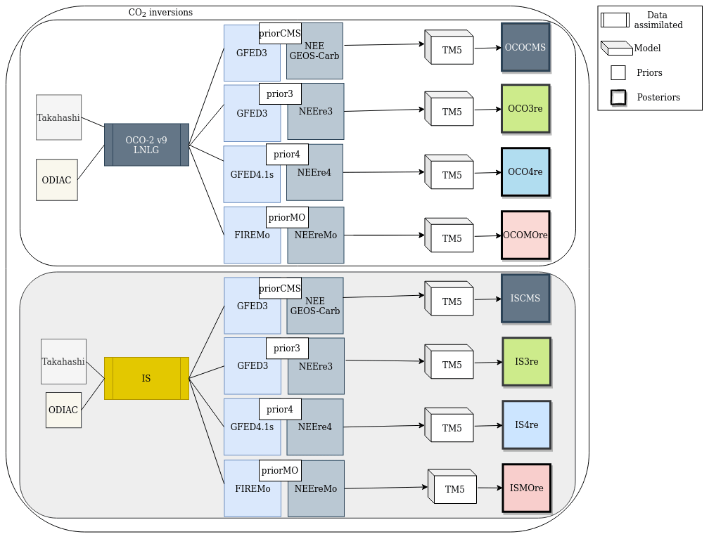
In this study, several inversions were performed with the TM5–4D-Var inversion framework. MOPITT v8 L2 CO data were assimilated to constrain fire emissions of CO. Separately, OCO-2 v9 XCO₂ and in situ CO₂ are used to constrain net fluxes of CO₂ (see Fig. 2).

Figure 2 Flowchart of the six different CO₂ inversions performed.

We optimized CO biomass burning emissions and CO₂ biospheric and oceanic emissions on a weekly basis.

3 Results

In Sect. 3.1, we examine the impacts of assimilating MOPITT v8 XCO observations on inferred fire CO emissions after vegetation partition and the comparison with the prior GFED4.1s CO emissions categorized by vegetation type.

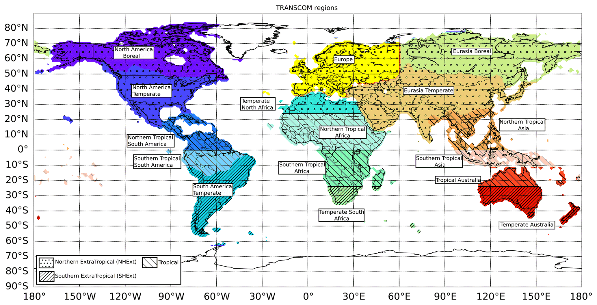
Figure 3 OCO-2 MIP (Model Intercomparison Project) regions for which prior and posterior gridded fluxes are aggregated for comparison.

In Sect. 3.2, we focus on the CO₂ inversions. As fire emissions are not optimized in CO₂ inversions, we examine how posterior NEE varies according to observation constraint and the imposed fire fluxes. We first compare (in Sect. 3.2.1) the variability and magnitude between the fire and biospheric priors used in the CO₂ inversions over the globe and zonal bands. Comparisons are also done over the same regions as in Crowell et al. (2019), which are TransCom (Gurney et al., 2002) regions that are further subdivided at the Equator (which we call OCO-2 MIP regions, where MIP stands for Model Intercomparison Project). The regions are defined in Fig. 3 and are composed of 16 land regions and 11 ocean regions. We focus on regions over land, as we are mostly interested in the interplay between assumed fire emissions and inferred NEE. We then investigate the covariation of imposed CO₂ fire emissions and optimized NEE with OCO-2 data and in situ data (Sect. 3.2.2). Finally, posterior simulated CO₂ mixing ratios are validated against TCCON data over the globe in Sect. 3.2.3.

3.1 Fire CO emissions partitioned by vegetation type: MOPITT optimized emissions versus GFED4.1s emissions

Figure 4 shows the annual CO posterior and prior fire emissions split by vegetation combustion across the globe and by OCO-2 MIP regions. Overall, it can be seen that, depending on the region, the assimilation of MOPITT data yields less or more CO emissions compared to the prior GFED4.1s.

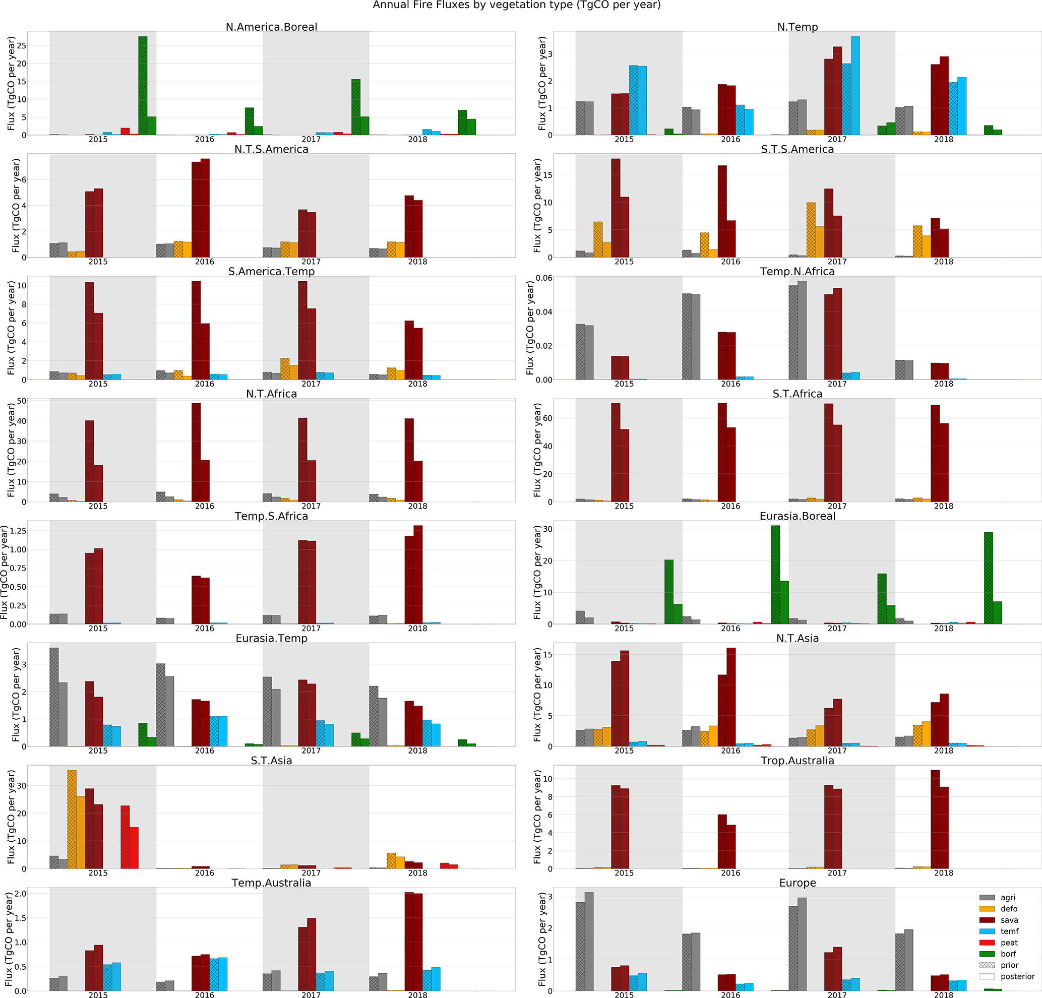
Figure 4 Annual CO fire emissions by vegetation type over the OCO-2 MIP regions between fire priors (hatch bars) and fire posterior from 2015 through 2018. Vegetation types are representing by colors: agriculture in gray, deforestation in yellow, savanna in dark red, temperate forest in blue, peatland in red, and boreal forests in green. Emissions are annually in Tg CO yr⁻¹.

For North America Temperate, posterior emissions remain close to the prior estimates, suggesting that the inferred emissions are consistent with GFED4.1s. Comparable results are also observed for Temperate North Africa. However, this region is known to have a lot of Saharan dust transported across the Atlantic Ocean and towards Europe most of the year, which could explain the posterior emissions being close to the prior as those MOPITT soundings have largely been removed by prescreeners. Northern Tropical Africa is not only affected by dust, but it is also largely affected by clouds during the wet season of the African monsoon (from May to August), which could lead to errors in retrievals that pass the prescreeners. The combination of clouds and dust could explain the MOPITT posterior fires having lower emissions than the prior GFED4.1s estimate. But further investigation into Northern Tropical Africa is needed. Even though the prior is higher than the posterior for Tropical Africa, in opposition to the previous multi-species study of Zheng et al. (2018a), the posterior emissions better fit MOPITT measurement than the prior (Fig. S4). Tropical South America (including Northern Tropical South America and Southern Tropical South America) is also known to have cloud coverage limiting satellite observations. We, however, observe similar emissions between the prior and the posterior for the northern region, with slightly higher emissions for MOPITT. For the southern region, differences between the prior and the posterior are large. The cloud coverage might explain this behavior, but further investigation is needed for these two regions.

The discrepancies observed for Eurasia Temperate between MOPITT and GFED4.1s could be that the vegetation type is not well represented for these regions. As mentioned in Pechony et al. (2013), agriculture and savanna vegetation types might not be the dominant burning vegetation type over North Africa and the Middle East, as these regions have seen an increase in croplands, controlled by human activities, and therefore rarely burn. However, Kazakhstan is a region of temperate forest often dominated by fires (Venevsky et al., 2019), a characteristic that is shared between the MOPITT constrained fire emissions and GFED4.1s.

We can also observe that over Northern Tropical Asia, MOPITT fire emissions are higher than GFED4.1s (see Figs. 4 and S6). This is observed for all years, where MOPITT emissions are almost 5 Tg CO yr⁻¹ (2 Tg CO yr⁻¹) for savanna (for the other vegetation types), which is higher than from GFED4.1s. As mentioned in Pétron et al. (2002) and Arellano et al. (2004), CO emissions in Northern Tropical Asia are significantly underestimated in current inventories. Previous studies have shown that the parameterization of peat (surface area and layer thickness) resulted in significant uncertainties in emission inventories. This is especially true for Indonesia (Lohberger et al., 2017; Hooijer and Vernimmen, 2013), where combustion of peat can produce a significant amount of carbon (Nechita-Banda et al., 2018). Our posterior fire emissions are lower than the prior fire emissions for Southern Tropical Asia, in contradiction to what Nechita-Banda et al. (2018) observed. However, Nechita-Banda et al. (2018) assimilated MOPITT and NOAA observations and used GFAS as a prior for fire emissions. Also, their inversion setup was different to what we used. Additionally, no evaluation against independent data have been performed in their study, so there is no reason to believe their results are more trustworthy than ours.

Moreover, our posterior can capture the seasonality of peat fires over Indonesia in comparison to GFED4.1s. Figure S5 shows for Southern Tropical Asia (mainly visible in 2015 due to the large emissions) that GFED4.1s have a fire peak earlier than MOPITT. van der Laan-Luijkx et al. (2015) and Nechita-Banda et al. (2018) hypothesized that GFED4.1s might not capture the timing of emissions over the area with peat fires due to the use of the burned area, which may be more sensitive to the initial stages of the fire than to the continued burning.

3.2 OCO-2 and in situ CO₂ inversions with different fire and NEE priors

We performed inversions with different CO₂ fire and NEE priors assimilating: (i) OCO-2 XCO₂ retrievals and (ii) CO₂ in situ data. See Fig. 2 for details of the eight CO₂ inversions.

To investigate the uncertainty in inferred CO₂ emissions arising from the selection of fires, we perform CO₂ inversions with three different global gridded fire estimates. The first one is taken from the GEOS-Carb CASA-GFED3 product (Ott, 2020), which we label “FIRE3”; for the second we use GFED4.1s, denoted “FIRE4”. The third set, denoted “FIREMo”, is described in “(b) Computation of an optimized CO₂ fire prior”. The methodological differences between FIRE3 and FIRE4 are described in Appendix A.

3.2.1 Prior NEE and fires CO₂ fluxes

Figure 5 shows annual CO₂ emissions for the prior estimates at a global scale and by latitude bands from 2015 through 2018. The prior categories shown are fire, NEE, and net fluxes for prior4 (FIRE4, NEEre4), prior3 (FIRE3, NEEre3), priorMO (FIREMo, NEEreMo), and priorCMS (FIRE3, GEOS-Carb). At the global scale, the three non-CMS priors (prior3, prior4, and priorMO) give the same net sink of carbon for the whole period (matching the AGR_NOAA with the same assumed fossil and ocean fluxes), increasing from 2015 through 2018. The priorCMS gives net sources of carbon increasing in time. Global fire emissions and net carbon fluxes, of the non-CMS priors, are within the spread of estimation of the Global Carbon Budget estimated by Le Quéré et al. (2018) and Bastos et al. (2018). The decrease (increase) in NEE sinks (net sources) for priorCMS during the period of study is driven by the fact that the product imposes a long-term balance between fire and NEE and is not constrained to match the measured growth rate of CO₂ in the atmosphere. The discrepancy shows up particularly in the Northern Hemisphere extratropics (NH Ext) and Southern Hemisphere extratropics (SH Ext), where sinks of priorCMS are generally smaller than the others.

Figure 5 Annual prior CO₂ emissions (Pg C yr⁻¹), at a global scale and by latitude bands, used later in top-down inversions. Annual net flux (lines), NEE (bars with hatches), and FIRE (bars with darker colors) prior emissions are shown from 2015 through 2018 (left to right) between prior4 (blue), prior3 (green), priorMO (red), and priorCMS (black).

We can observe that prior4 and priorMO have deeper Northern Hemisphere sinks than prior3 (particularly observed for Europe and northern Asia, Figs. 5 and 6), which is balanced by stronger net sources over the tropics (coming mainly from Southern Tropical Africa and Southern Tropical Asia respectively, Fig. 6). The scaling of GFED3 GEE and respiration to match the global AGR yields deeper biogenic sinks over the tropics than with all the other priors. We can also observe for Southern Tropical Africa that FIRE4 has larger fires than FIREMo.

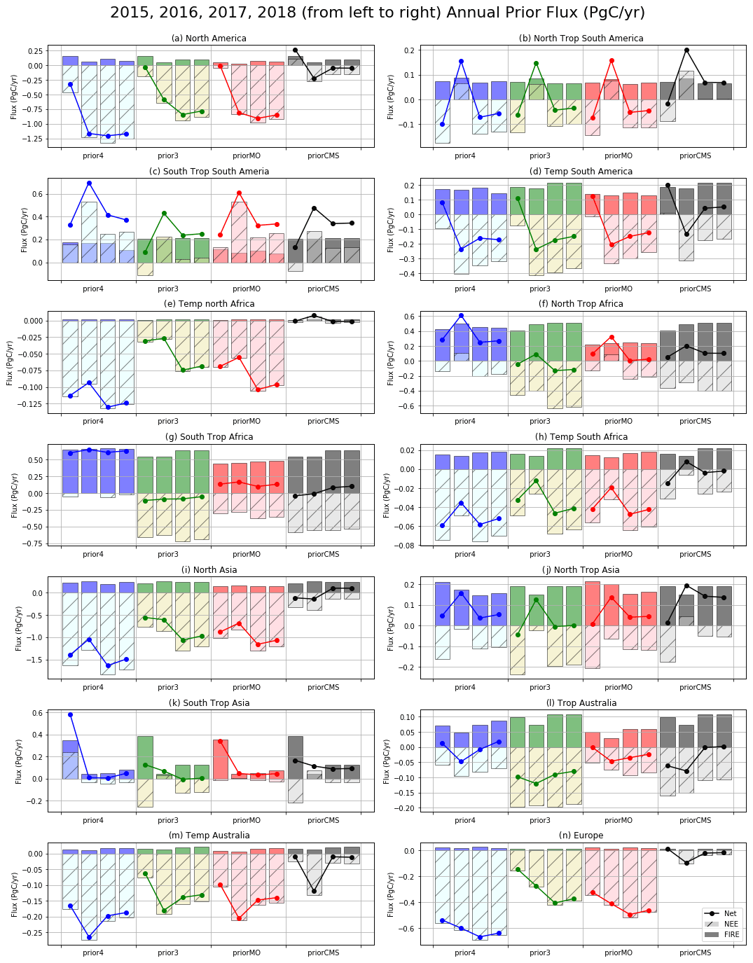
Figure 6 Same as Fig. 5 but for all OCO-2 MIP regions (from left to right, top to bottom): North America, Northern Tropical South America, Southern Tropical South America, South America Temperate, Temperate North Africa, Northern Tropical Africa, Southern Tropical Africa, Temperate South Africa, North Asia, Northern Tropical Asia, Southern Tropical Asia, Tropical Australia, Temperate Australia, and Europe.

The global fire emissions indicate that FIREMo yields fewer emissions compared to all other priors – a difference coming from tropical regions. These lower fire emissions estimated by FIREMo in the tropics come mainly from Tropical Australia (with values in 2015 of ∼0.05 Pg C yr⁻¹), Tropical Africa (∼0.35 Pg C yr⁻¹) and Southern Tropical South America (∼0.1 Pg C yr⁻¹). But larger fire emissions are observed with FIREMo in Southern and Northern Tropical Asia compared to FIRE4. The larger emissions with FIREMo compared to FIRE4 over Tropical Asia come mainly from savanna (the main vegetation type in this region; see Fig. S7).

As already observed with the CO emissions (Fig. S5) and discussed in van der Laan-Luijkx et al. (2015) and Nechita-Banda et al. (2018), the seasonality of fires over Tropical Asia seems to be better captured with MOPITT than with the CO emission inventories for peatlands. However, this is not only true for peat but also for other vegetation types and can also be observed for CO₂ emissions. For savanna, agriculture, and peatlands, FIREMo has a peak in fire seasonality after the peaks observed with both FIRE3 and FIRE4 (Fig. S8). This is particularly true for the 2015 El Niño fires but less for the fires that occurred in 2017 and 2018. In this period, FIREMo does not observe as much fire emissions as FIRE3 and FIRE4 with a similar seasonality. The large difference in seasonality for 2015 could be particularly marked due to the large and intense fires of the El Niño event burning larger regions and releasing more smoke. However, it is important to acknowledge the existence of data gaps due to clouds and smoke in both MODIS burned-area products (used in GFED3 and GFED4.1s inventories) and probably MOPITT retrievals. Further investigations are therefore needed for this region to make more conclusive remarks.

3.2.2 Posterior NEE and fire CO₂ fluxes

We assimilated OCO-2 and in situ data separately in order to assess the impact of these data in conjunction with different fire emissions and corresponding land flux priors. In all inversions, only NEE and ocean fluxes have been optimized.

(a) Global and latitudinal flux

Figure 7 shows global and latitudinal annual net fluxes, as well as FIRE and NEE fluxes for both OCO-2 and in situ (IS) inversions. We can see that, globally, net fluxes for OCO-2 posterior emissions across the different inversions are consistent. The sinks seem to adjust the different fire contributions. This is also observed for the IS inversions.

Figure 7 Global and latitudinal CO₂ posterior emissions for OCO-2 inversions as OCO4re (in blue), OCO3re (in green), OCOCMS (in black), and OCOMOre (in red) and in situ inversions (gray background). Annual fluxes are displayed from 2015 (a, c) through 2018 (b, d). FIRE emissions are the darker-colored bars, NEE fluxes are the hatched bars, and lines depict the net land fluxes.

The range of net flux observed with all OCO-2 inversions is consistent with other studies (Palmer et al., 2019; Crowell et al., 2019; Peiro et al., 2022). Global sinks are larger with IS inversions than with OCO-2 ones. These sinks observed with IS inversions are driven by larger sinks in the tropics (Fig. 7). OCOCMS and ISCMS posterior emissions seem to have slightly weaker sinks than the other posteriors. The imposed AGR seems to then have an impact at latitudinal scales.

The Northern Hemisphere extratropics (NH Ext) posterior fluxes are consistent across the different inversions for both observation constraints, which is not surprising given the good coverage of the in situ observations in this region. The consistency across the inversions for the northern latitude bands is also observed in the simulation study of Philip et al. (2019), where they used different NEE priors to observe the impact on the OCO-2 posteriors. For OCO-2 inversions, we can see small variations from year to year (going to −2.5 Pg C yr⁻¹ in 2015 through −2.75 Pg C yr⁻¹ in 2016) except for 2018 where the net sink drops to −2 Pg C yr⁻¹.

SH Ext shows similar fluxes across the inversions for each data constraint. However, the 2016 sink is larger for the OCO-2 fluxes (between −0.4 and −0.6 Pg C yr⁻¹) than the in situ fluxes (between −0.2 and 0.1 Pg C yr⁻¹), balanced with stronger sources over the tropics. This result suggests a transport connection between the tropics and SH Ext fluxes with the OCO-2 inversions, where land coverage is limited and hence retrievals are sparser than in the other regions. On the other hand, this does not seem to be the case in the in situ results, but we know that there are a few in situ sites present in the SH Ext, resulting in a limited constrain on emissions as well.

For the tropics, we can again observe a consistency in OCO-2 across the inversions. The intense fires and CO₂ sources related to the 2015 El Niño–Southern Oscillation over the tropics and mainly Indonesia might not be seen with in situ data due to their weak coverage in these regions. This could then explain the larger sinks with in situ observations. Even though we observe a consistency across the inversions, OCOMOre and ISMOre have a smaller sink in 2015 (with sources for OCO-2 inversion) compared to the other inversions in order to balance the 0.5 Pg C yr⁻¹ smaller fires that FIREMo gives. This balance was also observed for the priors (see Fig. 6). For the tropical regions, ISMOre and IS4re net fluxes look similar. Similarly, the inversions constrained with FIRE3 look alike, such as IS3re and ISCMS. This suggests the sensitivity of inversions to the fire prior in these regions.

(b) Regional fluxes

When we compare the posterior regional fluxes, we observe consistent differences in posterior NEE between IS and OCO-2 inversions. Some of these differences are caused by differences in data coverage and cloud fraction. If we look the northern extratropical regions, we can see that the IS inversions have deeper net sinks than OCO-2 (see Fig. 7). The in situ data place almost all of the NH Ext sink over northern Asia but place sources of carbon over North America for 2015 (Fig. 8). In situ data do not have a homogenized coverage over the NH Ext band: large number of observations are situated over North America Temperate and Europe but are very sparse over the boreal regions and Eurasia Temperate (see Fig. S1). The large differences in net sinks then occur over the regions where data are sparse (North Asia regions).

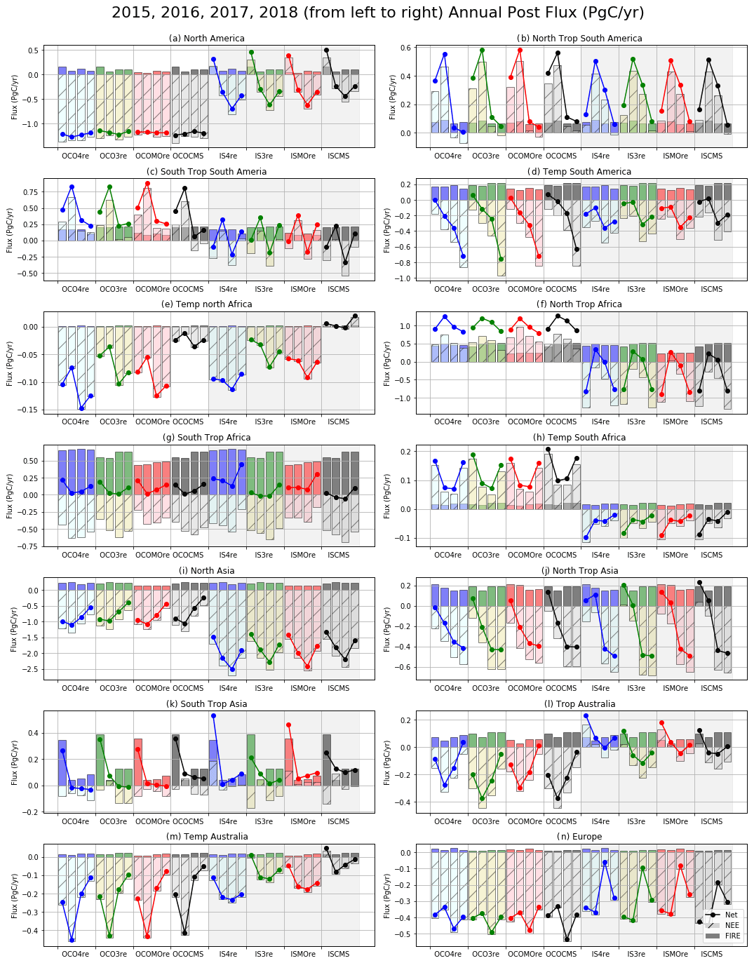
Figure 8 Same as Fig. 7 but for all OCO-2 MIP regions (from left to right, top to bottom): North America, Northern Tropical South America, Southern Tropical South America, South America Temperate, Temperate North Africa, Northern Tropical Africa, Southern Tropical Africa, Temperate South Africa, North Asia, Northern Tropical Asia, Southern Tropical Asia, Tropical Australia, Temperate Australia, and Europe.

Focusing on the tropical regions, OCO-2 fluxes are consistent for each inversions. For Northern Tropical South America (Fig. 8), OCO-2 fluxes have around 0.5 Pg C yr⁻¹ efflux during the El Niño period (2015–2016) and neutral emissions during the 2017–2018 period. IS fluxes are also strong during the El Niño period but remain moderately high in 2017. As observed in the Fig. 1 of the paper of Peiro et al. (2022), which used the same set of IS data, the number of IS data does not decrease significantly, meaning that changing observational coverage is not the cause of this behavior. The number of in situ observations is particularly low in the tropics compared to the extratropical Southern Hemisphere and Northern Hemisphere (Fig. 2 of Peiro et al., 2022). One possible explanation is the lag between flux in the tropics and observation coverage by the in situ network, which could be aliasing flux signals in time, though this hypothesis is difficult to test.

Very large differences between the IS and OCO-2 inversions appears for Southern Tropical South America (Fig. 8). The OCO-2 posterior emissions seem to be closer to the priors than the IS posterior emissions are. One explanation for that has been mentioned previously in Peiro et al. (2022). The cloud coverage above the moist Amazon decreases the amount of OCO-2 retrievals, while IS data are located more inside the moist Amazon.

For Northern Tropical Africa, net fluxes derived with OCO-2 are strong, with large sources of carbon between 0.5 and 1.5 Pg C yr⁻¹. We can see also some fire-dependent differences: posterior net sinks derived with FIREMo and FIRE4 emissions decrease for 2017; however, the posterior net sinks derived with FIRE3 do not. This difference in 2017 is particularly observed with OCO-2. IS inversions, on the contrary, give strong sinks in this region, with the strongest one for all tropical regions. Examining Fig. 6, we note the known prior dependency of the IS posterior emissions. Northern Tropical Africa is known to have very few IS data compared to the other tropical regions (Fig. S1).

Northern Tropical Asia (Fig. 8) shows agreements between OCO-2 and IS inversions but shows significant differences in 2016. The sparse coverage of in situ data over this region could explain the difference with OCO-2 but not specifically for 2016 alone, and hence further investigations are needed for this region.

It is also interesting to see the balance between the regions in the Northern Hemisphere and Southern Hemisphere. For instance, it seems that the sink reduction for 2018 (starting in 2017) observed with both IS and OCO-2 inversions over North Asia is balanced by net sinks in Tropical Asia (north and south). The deeper sinks observed with OCO-2 in Europe are also anti-correlated with the net sources observed in Northern Tropical Africa (Fig. 8). Reuter et al. (2014) found, using GOSAT data, a similar mass balance between Europe and northern Africa, with an uptake of around 1 Pg C yr⁻¹ in Europe, which was 0.5 Pg C yr⁻¹ higher than expected from in situ inversions. However, as mentioned in Reuter et al. (2017), there is a lack of carbon budget information over Europe, and there is hence no reliable benchmark for comparison. The balance observed here between IS and OCO-2 inversions was also observed in the study of Peiro et al. (2022). However, for Europe, we can see that the variability in our inversions is different than the ones used in Peiro et al. (2022). A major difference between this study and Peiro et al. (2022) is that the rebalanced priors and posterior fluxes provide the largest sink in 2017, as opposed to 2016 (see Figs. 6 and 8). This is likely a consequence of the larger fires and the subsequent rebalanced respiration that was derived in our study.

For all data constraints, we can observe a smaller sinks in the tropics during El Niño, while larger net sinks are observed in the NH Ext. In opposition to the other southern tropical regions, the El Niño–Southern Oscillation (ENSO) signal appears for Southern Tropical South America in 2016 instead of 2015 with OCO-2 inversions. This region follows the inter-seasonal variations of the northern tropical regions, which also see highest emissions in 2016. Moreover, larger sinks are observed with OCO-2 in North America and Europe, while larger sinks are observed with IS inversions in Asia.

Finally, the net fluxes using FIREMo look like those using FIRE4 for the southern tropical regions, while net fluxes using FIRE3 look alike, suggesting the sensitivity in these regions to the fire prior not only for IS data but also for OCO-2 data constraint. Across the different fire emissions, we observe a split: ISMOre and IS4re inversions provide similar results (both based on either optimized GFED4.1s and default GFED4.1s emissions), while the same is true for IS3re and ISCMS inversions (both based on GFED3 emissions). The same is true for OCO-2 inversions as well, where OCOMOre and OCO4re have similar results while OCO3re and OCOCMS are similar. That means fires have a larger impact on the posterior solution than the rebalancing of prior NEE to match the global AGR. We can observe that for almost all regions, the sinks with NEE4re and NEEreMo are deeper than with NEE3re and Geos-Carb CMS but are balanced with larger sources in other regions, mainly over the tropics (Fig. 7).

For Southern Tropical Asia, a smaller sink was derived with OCOMOre and OCO4re than with OCO3re and OCOCMS, to balance the smaller fires derived with FIREMo and FIRE4. This is not observed, however, for the IS inversions, which just show NEE sources for both ISMOre and IS4re. The impact of the fires over this region seems to have a strong impact with both data constraints. If we compare the posteriors with the priors, we can in fact see that the IS inversions tend to be closer to the priors than the OCO-2 inversions. This suggest that for this region as well, the few number of IS data might explain this result, and the larger number of OCO-2 data seem to better constrain the posterior fluxes.

For Southern Tropical Africa, we can see the large balance between the fires and the NEE emissions (indirectly the balance between the fires and the respiration), which are anti-correlated in their variability. Additionally, OCO-2 inversions derived with FIREMo and FIRE4 emissions (OCOMOre and OCO4re) have larger sources than inversions derived with FIRE3 (OCOCMS and OCO3re). With the IS inversions, there is large variation across the inversions where IS4re and ISMOre both constrain a source of carbon for the whole period, while ISCMS and IS3re have smaller source of carbon and even a sink in 2016 and 2017. These differences between inversions derived with FIREMo, FIRE4, or FIRE3 seem to suggest that fires (and thus NEE rebalanced with fires) are especially important when observational coverage is limited.

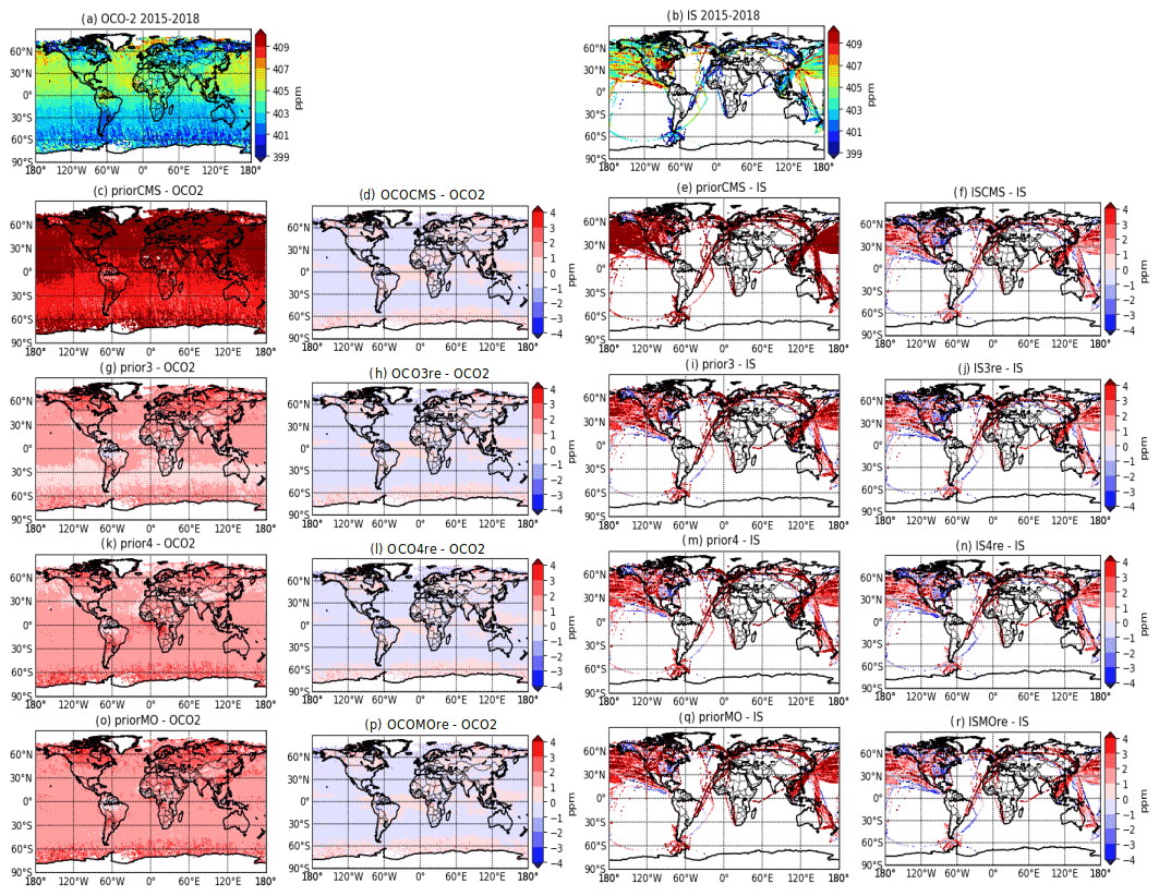
Figure 9 Spatial distributions of the CO₂ total column (XCO₂). Mean distribution of OCO-2 retrieval (a) and in situ data (b) over the 2015–2018 period. Each simulation are displayed by row (priorCMS, c–f; prior3, g–j; prior4, k–n; and priorMO, o–r). Annual difference between the prior of each simulation minus OCO-2 data (in panels c, g, k, and o) and minus IS (in panels e, i, m, and q). Annual difference between the posterior simulation of each simulation minus OCO-2 (in panels d, h, l, and p) and minus IS (in panels f, j, n, and r). Results are in parts per million (ppm).

3.2.3 Evaluation of the simulations

3.2.4 (a) Evaluation of the inversions to fit the OCO-2 retrievals and IS data

The global distributions of OCO-2 retrievals over the 2015–2018 period (Fig. 9a) show latitudinal gradients from north to south, with higher XCO₂ concentrations in the tropics and the Northern Hemisphere. High concentrations over land (no higher than 409 ppm) are observed over East Asia, northwest Africa, and Northern Tropical South America. Figure 9b shows the global distributions of IS data with a higher number of observations in the Northern Hemisphere than the tropics or the Southern Hemisphere. High XCO₂ concentrations (higher than 409 ppm) can be observed for North America Temperate and near the coast of East Asia. The regional mean differences between the prior or posterior with either the OCO-2 retrievals or IS data are summarized in Table S1 in the Supplement.

The priors have larger differences with the OCO-2 retrievals than the posteriors. The prior3 (using both FIRE3 and NEEre3; see Fig. 2) better fits the OCO-2 measurements than the other priors for the Southern Hemisphere and the tropics (Fig. 9 and Table S1). The priorCMS, however, does not fit the OCO-2 measurements with high bias between 3 and 4 ppm. The large difference is also observed with the IS measurements. For the IS inversions, the differences between priors and posteriors are very similar, suggesting that the inversion does not change much from the prior. The small number of observations available in these regions could explain this result. While the optimized concentrations fit the OCO-2 retrievals quite well compared to the priors, suggesting the inversion’s ability to fit the data. Among the different simulations, in particular, the posterior concentrations vary little in comparison to OCO-2 and IS data.

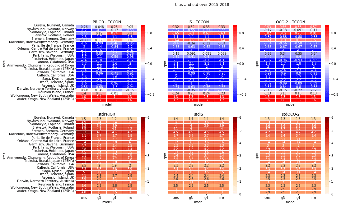
Figure 10 Comparison between TCCON data and the prior (left column), IS simulations (center column), and the OCO-2 simulations (right column). Top panels show experiments biases, and bottom panels show standard deviation compared to TCCON sites. Biases and standard deviation are expressed in ppm CO₂. The left column from left to right shows the priors priorCMS, prior3, prior4, and priorMO. The center column from left to right shows the simulations ISCMS, IS3re, IS4re, and ISMOre. The right column from left to right shows the simulations OCOCMS, OCO3re, OCO4re, and OCOMOre.

3.2.5 (b) Validation against TCCON data

As mentioned previously, most of the differences observed between in situ and OCO-2 inversions could be due to their respective coverage. In situ measurements have fewer data over the tropics and Southern Hemisphere than OCO-2 retrievals. However, besides the spatial coverage, satellite retrievals might be affected, particularly over the tropics, by the consistently cloudy region known as the Intertropical Convergence Zone (ITCZ) as well as aerosols from biomass burning or dust (such as over and near the Sahara). It is then important to validate the OCO-2 and in situ posterior simulated mixing ratios against independent data. In this section, in order to explore the accuracy in the posterior fluxes, we evaluated the posterior fluxes by sampling the resultant concentrations for comparison with TCCON measurements. All posterior mixing ratios have been sampled around TCCON retrieval locations and times using the appropriate averaging kernels.

In comparison to TCCON, for the 2015–2018 period, the CO posterior biases were underestimated by 7 ppb, while the CO priors were overestimated by 13 ppb (Fig. S9). Even if the posterior biases are lower than the prior biases, the underestimation observed in Fig. S9 against TCCON could explain the low fluxes observed of the FIREMo compared to the other fire estimates over some regions. We can observe an underestimation of the posterior CO mixing ratio of $\sim -\mathrm{12}$ ppb in 2015 at the Ascension Island site, while the a priori CO mixing ratio has an overestimation of 5 ppb in 2015. However, the biases at the Darwin TCCON site give −3 ppb for 2015–2016 (−0.5 ppb for 2017–2018) with the posterior and 20 ppb for 2015–2016 (22 ppb for 2017–2018) with the prior. This gives the impression that our inversion is not getting the best fluxes for Ascension Island, but we can see that this is not the case for other tropical locations. Ascension Island is known to be impacted with Saharan dust, and therefore the posterior simulated concentration could be biased due to aerosols.

Figure 10 shows biases between the prior and posterior simulated mixing ratio (XCO₂) of the different CO₂ inversions against each TCCON sites. While the priorCMS has the largest biases with TCCON and standard deviation, the other priors used (prior3, prior4, and priorMO) have biases and standard deviation very close each other for most of the sites. Improvements of biases and standard deviation with the prior3 compared to priorCMS, which also use FIRE3 as fire prior, are likely due to the rebalanced respiration that matches the NOAA growth rate. This rebalanced respiration and growth rate have also been used for prior4 and priorMO. While the rebalanced prior mixing ratio is relatively similar, prior4 and priorMO have lower biases than prior3. Additionally, depending on the TCCON site, priorMO biases are slightly smaller than prior4. It is then not straightforward to conclude which rebalanced prior is doing better than the others. The XCO₂ posteriors are in better agreement with TCCON measurements than the priors. Biases observed with OCOCMS and ISCMS have been greatly reduced by the inversion, compared to priorCMS, with biases of the same order as compared to the other inversions. For the posterior simulated mixing ratio with IS data, we can see that all biases are very similar among the simulations, and it is here again difficult to conclude which posterior does best. On average, IS4re seems to do better, but, looking site by site, ISMOre provides a better match at some tropical sites than the other simulations (such as for Ascension Island and Reunion Island). The same applies for the posterior simulated mixing ratio with OCO-2 data, where there is not one simulation doing better than the others on average. Additionally, all standard deviations are similar between all inversions, with a slightly larger standard deviation for the IS inversions than for the OCO-2 inversions.

We observed in the results section that posterior fluxes had similarity across the inversions used for each data constraints for SH Ext (see Fig. 7), but 2016 is adjusted downward significantly in the OCO-2 fluxes. Evaluation against the two TCCON sites in the SH Ext shows similarity using either IS or OCO-2 constraint (1.3 ppm biases) for Wollongong, but biases are slightly lower with OCO-2 fluxes for Lauder (1.6 ppm with OCO-2 fluxes against 1.7 ppm for IS fluxes). For NH Ext, we observed previously (see Fig. 7 for North America and Europe mainly) a strong sink for OCO-2 over the period compared to IS inversions, which observed stronger year-to-year variability. The evaluation with TCCON data at European sites shows smaller biases using IS data than OCO-2 data for all simulations. For instance, at the Garmisch site, biases are around −0.1 and −0.34 ppm with IS fluxes and OCO-2 fluxes respectively, showing a larger underestimation with OCO-2 than IS fluxes. But for the North American sites, biases are lower with OCO-2 fluxes than IS fluxes (see the Lamont site for instance in Fig. 10).

4 Discussion

In this study, we have presented an optimized CO₂ fire prior flux based on the emission ratio between CO₂ and CO that comes from optimized CO fire emissions using MOPITT CO retrievals. In addition, as fire emissions and plant respiration (terms included in the net fluxes) are difficult to disentangle, we rebalanced the respiration with each fire emission estimate and with the annual NOAA growth rate. We then explored a range of NEE emissions based on different fire emissions including a CO₂ fire estimate calculated from CO fire emission information in order to better constrain biospheric emissions. We focused our study for the period 2015–2018 to observe the impact of the El Niño event in 2015 and the recovery period that followed.

Globally and for most regions, we find that the inversion results have a greater dependence on data constraint than on prior emissions. The variations in posterior flux are much smaller across different prior mean fluxes (and the different uncertainties that come from scaling the prior mean flux) as compared with differences resulting from assimilating OCO-2 versus in situ data. There are exceptions, most notably in the northern and southern tropics, where the in situ constraint is especially limited and the corresponding posterior annual fluxes vary by as much as 0.5 Pg C, which is a large fraction of the expected total El Niño signal. This suggests that in situ constrained flux estimates in the tropics are more sensitive to the assumed prior flux, of which fires are a significant component, and should be assigned the appropriate amount of uncertainty in accordance with this finding. It also implies that while residual biases in satellite retrievals remain a key focus of the top-down inversion community, further work is needed to improve prior fluxes in tropical regions as well as deploy more in situ measurements. Current efforts by multiple organizations should assist in that effort on a short-term basis, but more investments in long-term monitoring are needed (Kathryn McKain, personal communication, 2021). OCO-2 inversions are also sensitive to the prior assumption in northern Africa, though to a lesser extent, as well as in Tropical Asia. Tropical Asia has been particularly well studied in the past, where Nechita-Banda et al. (2018) and van der Werf et al. (2017) have shown the underestimation of GFED inventories of peat fires compared to space-based instruments such as IASI and MOPITT. This reinforces the need for better measurements and bottom-up estimates of biospheric and fire fluxes in these tropical regions. Nechita-Banda et al. (2018) converted their CO fire emissions in CO₂ emissions using emission factors and estimated that a range of 0.35–0.60 Pg C was emitted in Indonesia and Papua from the 2015 fires. We calculated our fire CO₂ emissions over the same region and found 0.41, 0.37, and 0.39 Pg C for FIRE3, FIRE4, and FIREMo respectively. Our fire CO₂ estimates are hence in agreement with those found by Nechita-Banda et al. (2018). As mentioned previously, we know that GFED4.1s has information of small fires compared to GFED3 which allow better accuracy particularly over the tropics where peat fires are important. However, we can see lower FIRE4 emissions than FIRE3 for Southern Tropical Asia, similarly to what Shi et al. (2015) found for the 2002–2012 period. A possible explanation could be that the CASA biogeochemical model of GFED3 predicts higher biomass densities than with the new version used in GFED4. Validation against fuel loads measured in savanna and grassland fields was found to be higher with GFED3 than with GFED4.1s (Randerson et al., 2012; Giglio et al., 2013). In 2015, during the onset of the El Niño event which caused intense fires over Indonesia, FIREMo emissions are stronger than with FIRE4 emissions but lower than with FIRE3 emissions. Fires over peatlands spread more during the El Niño event due to intense drought conditions (Nechita-Banda et al., 2018). Consequently, they emit 2 to 4 times more CO than forest fires (Akagi et al., 2011) and contribute significantly to the exchange between terrestrial carbon stocks and the atmosphere by decreasing the uptake of atmospheric CO₂ by the biosphere. This is particularly shown for the IS inversions where IS4re and ISMOre provide higher net carbon sources compared to the IS inversion constrained with GFED3 fires. Moreover, FIREMo was able to catch the seasonality of fires over Southern Tropical Asia during the El Niño event, compared to the other priors using GFED inventory. As discussed in Nechita-Banda et al. (2018) and van der Laan-Luijkx et al. (2015) for equatorial Asia and Tropical South America, GFED4 does not capture fire seasonality due to the use of burned area, compared to GFAS. In both the GFED and GFAS method (and similarly for MOPITT), the detection of fires underneath clouds and below the canopy is difficult. But FIREMo, compared to FIRE3 and FIRE4, has the advantage of combining optimized fire emissions with local observations. It is thus important to use CO observations to constrain estimates of CO₂ fire emissions and subsequently constrain NEE with OCO-2 and IS observations. But uncertainty in our emission ratio remains when converting CO to CO₂ emissions in our prior. GFED vegetation partition only accounts for six different types of vegetation which might not be fine enough to represent all different types of fuels. Additionally, the emission factors, used in the emission ratio, lack spatial and temporal variability to account for the full dynamic range of combustion characteristics. We know, for instance, that African savanna fires can go from flaming to smoldering, changing the combustion efficiency (Zheng et al., 2018b) and hence the $\mathrm{CO}/{\mathrm{CO}}_{\mathrm{2}}$ emission ratio. This could explain the differences observed over some regions of the tropics between FIREMo and the other prior fire CO₂ emissions. The estimation of EF and consequently the emission ratio $\mathrm{CO}/{\mathrm{CO}}_{\mathrm{2}}$ cannot be determined accurately in the field and can introduce systematic errors in the EF(CO₂) values that may well exceed 10 %. One challenge is the separation of the information between small-fire inputs of CO₂ (and hence their detection) from large biospheric variability. Other difficulties come from the issue of variable background concentrations and from smoldering emissions that are not projected into the smoke plumes (Guyon et al., 2005; Burling et al., 2011; Yokelson et al., 2013). More work is required to improve emission ratios and particularly emission factors over different spatial and temporal scales. A recent study has shown that MODIS products most likely underestimate burned area for Africa (Ramo et al., 2021). The higher fire posterior emissions estimated in previous studies using GFAS as a prior compared to GFED4 (Nechita-Banda et al., 2018) and the results of Ramo et al. (2021) seem to suggest, for future work, the careful selection of the CO fire prior for the inversions. Some of our future works will focus on comparing different CO posterior emissions.

The data used to constrain inversions is very important. We could see up to 0.4 Pg C yr⁻¹ differences between OCO-2 and IS inversions in tropical regions. This bring us to the importance of the data assimilated in the inversions but also about the priors used in the inversions concerning the different sectors (fire and terrestrial emissions).

The difference in partitioning of fluxes in latitude and longitude for the different data constraints is not a new observation and fits the findings of the v7 OCO-2 MIP (Crowell et al., 2019) and previous studies comparing GOSAT and in situ data (Reuter et al., 2014; Houweling et al., 2015)) as well as of the v9 OCO-2 MIP, an extension of the v7 OCO-2 MIP (Peiro et al., 2022). More specifically, the OCO-2 data constrain a stronger northern extratropical sink in concert with a strong tropical source, while the in situ data generally constrain a weaker northern sink and neutral tropical flux, or even a sink. While the northern extratropics are relatively densely sampled by the in situ network, Schuh et al. (2019) found a strong sensitivity of flux estimates to model transport, particularly in the vertical and meridional transport of CO₂. Though we utilized only TM5 in these experiments, the findings here are consistent with those found in their study.

Regarding the question of the importance of the prior and the question of which prior could do better than the others, we have seen through the results and the evaluation that no simulation is better than the other on average. Even if the biases seem to have been reduced with priorMO for certain sites (such as Ascension Island for instance), they are in the same order as the other a priori biases for other site. On average and overall, the added value of optimizing fire emissions before optimizing NEE is not very apparent. Our results seem, overall, to be very insensitive to optimized fire emissions. Philip et al. (2019) performed simulation experiments with different NEE priors and concluded that posterior NEE estimates are insensitive to prior flux values. But they found large spread among posterior NEE estimates in regions with limited OCO-2 observations. Our results suggesting that OCO-2 inversions are relatively insensitive to the prior in most regions are consistent with Philip et al. (2019) and not only for OCO-2 inversions but also for IS inversions.

A generally accepted (though not documented) assertion is that a minimal number of data are required to constrain the global growth rate, and yet we see here that OCO-2 and the global in situ network do not see the same global annual flux, even assuming the same transport and prior flux that matches the AGR_NOAA. Part of this discrepancy is certainly due to the following: (i) most of the in situ measurements assimilated here are taken in the atmospheric boundary layer, while OCO-2 represents a column density; and (ii) most of the in situ measurements are in the northern extratropics, whereas OCO-2 measurements are globally distributed, but with seasonally varying coverage. Persistent transport biases as well as satellite retrieval errors likely play a factor in this global offset, though further investigation is necessary to assess the relative importance of each.

5 Conclusions

In this study, we have explored the potential of using the $\mathrm{CO}/{\mathrm{CO}}_{\mathrm{2}}$ emission ratio to add CO fire information in CO₂ inversions in order to better estimate and constrain CO₂ biospheric emissions. Fires have the potential to influence inter-annual variability and long-term trends in atmospheric CO₂ concentrations and particularly alter the seasonal cycle of net biome production. CO measurements are available with high precision from space and bring more accuracy in CO fire emission estimates. Including more accurate fire emissions in CO₂ inversions could improve the estimates of CO₂ land fluxes relative to a CO₂ inversion without the added information of CO. In this paper, we showed how we added on a global scale the $\mathrm{CO}/{\mathrm{CO}}_{\mathrm{2}}$ emission ratio and its respective rebalanced respiration with fire and NEE with annual NOAA growth rate, as well as its value for CO₂ inversions.

We performed several CO₂ transport inversions assimilating separately OCO-2 data and in situ measurements from 2015 through 2018. We found that OCO-2 and in situ net fluxes have a better agreement at the global scale as observations are dense enough to constrain the fluxes than at latitudinal and regional scales. Differences in net fluxes are particularly important over the tropics not only between OCO-2 and in situ inversions but also between the different priors used. Discrepancies occurred over Northern Tropical Africa where OCO-2 inversions derived net sources while in situ inversions derived sinks. However, over southern tropical regions, discrepancies appear between the different priors, with larger net sources derived with the OCO-2 inversion using the optimized fire emissions (OCOMOre) over Southern Tropical South America and with IS inversion over Southern Tropical Asia. For Tropical Asia, the priors seem to be more important than the data assimilated. Additionally, over this region, seasonality from CO₂ inversions using MOPITT fires seems to better represent the large Indonesian fires that occurred during the 2015 El Niño event.

TCCON evaluation suggested that the prior using FIREMo (CO₂ fire prior emissions computing using the $\mathrm{CO}/{\mathrm{CO}}_{\mathrm{2}}$ emission ratio) gives an accuracy in the CO₂ mixing ratio comparable to GFED4 but with slightly larger biases over the Northern Hemisphere. Biases of the priors with the rebalanced respiration are smaller than the CMS prior. Evaluation against TCCON shows smaller biases for all the rebalanced posterior simulated mixing ratios in comparison to the CMS posterior simulated mixing ratio. Additionally, the variability of all the rebalanced mixing ratios better matches that of TCCON. This suggests the importance of the accuracy in fire priors and the rebalanced of terrestrial emission with fires for the estimation of CO₂ posteriors emissions. However, the added value of CO fire emissions for NEE optimization is not significant in terms of bias reduction on average.

We illustrated the potential of using the $\mathrm{CO}/{\mathrm{CO}}_{\mathrm{2}}$ emission ratio and the rebalanced respiration with fire in order to match the atmospheric growth rate in CO₂ inversions. This was performed for better constraint and accuracy in the CO₂ fire prior emissions and biospheric emission estimates. We found that CO₂ fluxes are more robust if the NEE and fire emissions are rebalanced in order to match the AGR_NOAA. However, a more reliable NEE is obtained with the assimilated data, using either in situ or satellite-based CO₂ constraints. This opens new avenues for future research for the development of a joint CO–CO₂ inversion framework that uses multiple streams of data to improve the fire and biosphere emissions. Besides, the multi-species approach employing CO and CO₂ for instance is important for the interpretation of upcoming satellite data such as data from the upcoming NASA Earth Venture Mission, GeoCarb.

Appendix A: GFED versions descriptions

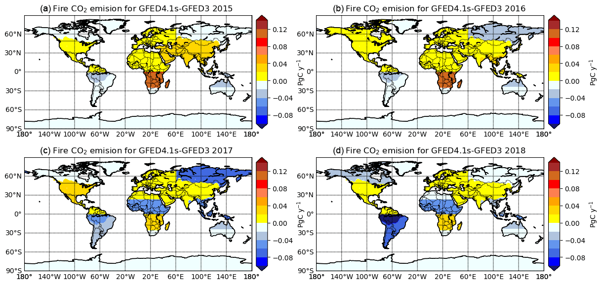
Figure A1 Annual differences between FIRE4 and FIRE3 in Pg C yr⁻¹ over the regions of Fig. 3 for (a) 2015, (b) 2016, (c) 2017, and (d) 2018.

The first version of GFED was released in 2004. Since then, several improvements have been incorporated into GFED. Improvement on the mapping of burned area from active fire data in GFED2 (Giglio et al., 2006) was no longer necessary when the MODIS product became available for GFED3 (Giglio et al., 2010). Burned area particularly affects the spatiotemporal variability of carbon emissions during fires. This spatiotemporal impact has been implemented in GFED with the biogeochemical modeling framework providing estimation of biomass combustion over different vegetation types (Giglio et al., 2013). All GFED versions are then based on the Carnegie–Ames–Stanford Approach (CASA) model adjusted to account for fires (see van der Werf et al., 2004, and van der Werf et al., 2017, for more details). The most recent versions (GFED4 and GFED4.1s, which includes the small-fire burned area) modified the burned-area-to-burned-fraction conversion, which has been shown to increase burned-area and fire carbon emissions by 11 % in GFED4.1s compared to GFED3 (van der Werf et al., 2017) at the global scale. Liu et al. (2017b) found that with the omission of small fires in GFED3, global fire emissions are underestimated. Accounting for small fires increased global burned-area and carbon emissions by 35 % (Randerson et al., 2012) and improved the agreement of spatial distribution between active fires and burned area over regions with large fires such as savanna fires and boreal forests. Including small fires in GFED amplifies emissions over regions where drought stress and burned area varied considerably from year to year in response to, for instance, the El Niño–Southern Oscillation (ENSO). The GFED4.1s version has encountered some changes since 2017 because the MODIS burned-area algorithm has been updated from Collection 5 to Collection 6. Consequently, GFED4s fluxes are no longer based on the burned-area product directly but on the relationship between climatological GFED4s emissions between 2003–2016 and active fire detection and the MODIS FRP product. The active fire data come from Tropical Rainfall Measuring Mission (TRMM), the Visible and Infrared Scanner (VIS), and the Along-Track Scanning Radiometer (ATSR), three other instruments on board with MODIS. MODIS has a 500 m horizontal resolution.

Figure A1 shows annual differences between FIRE3 and FIRE4 from 2015 through 2018 over the OCO-2 MIP regions. We note that regional differences are as large as 0.14 Pg C yr⁻¹, or roughly ∼10 % of the annual global fire emissions budget, which has been estimated to be 1.6±0.7 Pg C yr⁻¹ (Friedlingstein et al., 2020). Additionally, the size and sign of the differences vary by year and by region. For instance, FIRE3 generally predicts higher CO₂ emissions over the boreal regions, while FIRE4 (GFED4.1s) largely predicts more fire emissions from the northern midlatitudes. This is consistent with differences between the two models; i.e., GFED4.1s uses a different set of emission factors separating trace gas emissions and aerosol from boreal forest to temperate forests (Akagi et al., 2011; van der Werf et al., 2017). van der Werf et al. (2017) have shown that GFED3 does not capture the different patterns of fire severity between the boreal regions of North America and Eurasia and the differences between boreal and temperate forests fires (which could explain the large difference between FIRE4 and FIRE3 in Fig. A1). In addition, van der Werf et al. (2017) found that including the small-fire burned area in GFED4 doubled the burned area in North America Temperate and Europe compared to GFED3. Interestingly, the differences in the tropics have a pronounced zonal structure, where GFED4.1s predicts smaller emissions in South America, Tropical Asia, and North Africa (after 2016) and larger emissions in Southern Tropical Africa. The addition of the small-fire burned area included in GFED4.1s has a strong impact in the Southern Tropical Africa regions where agricultural waste burning and shifting cultivation are important drivers of fire activity. van der Werf et al. (2017) have shown that the increase of burned area in these regions was associated with the small-fire burned area from the last GFED version. Small fires linked with deforestation and agricultural waste are also important over Indonesia; however, deforestation activity decreased by almost 50 % in 2017 and 2018 thanks to several Indonesian policies in order to prevent forest fires and land clearing, with the new law in particular preventing the clearing of forest for oil palm plantations (Global Forest Watch, 2020). This might explain the decrease in fire emissions over Southern Tropical Asia in 2017 and 2018 with GFED4.1s, as well as the fact that 2017 and 2018 were not impacted by the 2015 El Niño event where large fires burned in Indonesia.