Combining short-range dispersion simulations with fine-scale meteorological ensembles: probabilistic indicators and evaluation during a ⁸⁵Kr field campaign

Numerical atmospheric dispersion models (ADMs) are used for predicting the health and environmental consequences of nuclear accidents in order to anticipate countermeasures necessary to protect the populations. However, these simulations suffer from significant uncertainties, arising in particular from input data: weather conditions and source term. Meteorological ensembles are already used operationally to characterize uncertainties in weather predictions. Combined with dispersion models, these ensembles produce different scenarios of radionuclide dispersion, called “members”, representative of the variety of possible forecasts. In this study, the fine-scale operational weather ensemble AROME-EPS (Applications of Research to Operations at Mesoscale-Ensemble Prediction System) from Météo-France is coupled with the Gaussian puff model pX developed by the IRSN (French Institute for Radiation Protection and Nuclear Safety). The source term data are provided at 10 min resolution by the Orano La Hague reprocessing plant (RP) that regularly discharges ⁸⁵Kr during the spent nuclear fuel reprocessing process. In addition, a continuous measurement campaign of ⁸⁵Kr air concentration was recently conducted by the Laboratory of Radioecology in Cherbourg (LRC) of the IRSN, within 20 km of the RP in the North-Cotentin peninsula, and is used for model evaluation.

This paper presents a probabilistic approach to study the meteorological uncertainties in dispersion simulations at local and medium distances (2–20 km). First, the quality of AROME-EPS forecasts is confirmed by comparison with observations from both Météo-France and the IRSN. Then, the probabilistic performance of the atmospheric dispersion simulations was evaluated by comparison to the ⁸⁵Kr measurements carried out during a period of 2 months, using two probabilistic scores: relative operating characteristic (ROC) curves and Peirce skill score (PSS). The sensitivity of dispersion results to the method used for the calculation of atmospheric stability and associated Gaussian dispersion standard deviations is also discussed.

A desirable feature for a model used in emergency response is the ability to correctly predict exceedance of a given value (for instance, a dose guide level). When using an ensemble of simulations, the “decision threshold” is the number of members predicting an event above which this event should be considered probable. In the case of the 16-member dispersion ensemble used here, the optimal decision threshold was found to be 3 members, above which the ensemble better predicts the observed peaks than the deterministic simulation. These results highlight the added value of ensemble forecasts compared to a single deterministic one and their potential interest in the decision process during crisis situations.

1 Introduction

Accidental releases of radioactive pollutants into the atmosphere can have a serious impact on human health and environment (Aliyu et al., 2015; Nie et al., 2021). The dispersion of radionuclides released into the atmosphere depends on the physicochemical properties of the released substances, the emission parameters (e.g., source elevation, timing, and duration of the release), and meteorological conditions at the accident site (e.g., wind speed and direction) (Girard et al., 2014). In order to forecast the dispersion of radionuclides during the early phase of nuclear accidents and to support decisions and warnings, atmospheric dispersion models (ADMs) are commonly used to predict the transport of radioactive pollutants through the atmosphere as well as the quantities of radioactive material deposited on the ground (Korsakissok et al., 2013). This information is essential for decision makers in order to anticipate the countermeasures necessary to protect the population against contamination.

1.1 Uncertainties and ensemble simulations

The outputs from ADM simulations suffer from significant uncertainties that limit the confidence in them when they are used in an operational context (Korsakissok et al., 2020; Leadbetter et al., 2020). The three main sources of these uncertainties have been discussed by Rao (2005) and by Mallet and Sportisse (2008). The first one is related to the source term, which is an essential input data. For a prognosis of potential releases, it may be defined from a priori assumptions (pre-defined source term), modeling of physical processes at stake within the reactor, along with knowledge of the damaged installation status. In case of an ongoing or past release, when observations are available in the environment, the source term can be reconstructed by inverse methods. For this purpose, IRSN (French Institute for Radiation Protection and Nuclear Safety) has developed inverse modeling methods, which are methods based on mathematics that aim to minimize the difference between ADM outputs and in situ measurements (Saunier et al., 2013, 2020).

The second main source of uncertainty is related to the meteorological forecasts that are given as input to ADMs. Weather information used for dispersion prediction is, frequently, provided by numerical weather predictions (NWPs) as 3D or 4D physical fields. To take into account the meteorological uncertainties on dispersion simulations, two methods have commonly been used. The first method is the addition of random perturbations to weather inputs (Girard et al., 2014, 2020). The second one is the use of meteorological ensembles (Straume et al., 1998).

Some studies have used operational ensemble prediction systems (EPS) as input for dispersion models in the case of the Fukushima accident (Sørensen et al., 2016; Kajino et al., 2019; Le et al., 2021), while others used EPS for hypothetical nuclear accident scenarios (Sørensen et al., 2019, 2020; Korsakissok et al., 2020; Leadbetter et al., 2022). These studies include either meteorological uncertainties only, or sometimes both meteorological and source term uncertainties. All these studies were carried out at long distance and the ensembles used to represent weather uncertainties had coarse spatial and temporal resolutions, except Leadbetter et al. (2022), who also used fine-scale weather ensembles with a horizontal resolution of about 2.5 × 2.5 km and 70 vertical levels. For example, De Meutter et al. (2016) studied the use of meteorological ensembles at hemispheric scale to predict radioxenon peaks coming from radiopharmaceutical facilities, and De Meutter and Delcloo (2022) studied it at continental scale for the same application, using the ECMWF-ERA5 ensemble at a horizontal resolution of 63 km. In the case of the Fukushima disaster in Japan, Le et al. (2021) investigated the dispersion of radionuclides using the operational ECMWF-ENS (Leutbecher and Lang, 2014) with a spatial resolution of approximately 25 × 25 km and 3 h time steps, using several source terms from literature. In Le et al. (2021) and De Meutter and Delcloo (2022), an evaluation of the dispersion ensembles was performed by comparison to radiological observations in the environment and the results illustrate the added value of the use of weather ensembles for dispersion simulations. In a hypothetical case study, Leadbetter et al. (2022) explored the uncertainties coming only from weather conditions at synoptic scale, by using the operational Met Office's EPS named MOGREPS-G (Tennant and Beare, 2014) with a spatial resolution of approximately 20 × 20 km and 3 h time steps. Although this approach allowed the demonstration of the ability of meteorological ensembles to perform atmospheric dispersion results more skillfully than results produced with deterministic meteorology, it did not evaluate the performance of the ensemble dispersion simulations in the case of a realistic release. While most applications of meteorological ensembles cited above were focused on hemispheric or continental scale, the impact of meteorological uncertainty on dispersion forecasts at local scale (in the range of 2 to 20 km) has received less attention. With the development of kilometer-scale EPS (Bouttier et al., 2012), the feasibility and interest for such studies are rising. High-resolution meteorological ensembles were used in the case of a fictitious nuclear release (Sørensen et al., 2017, 2020; Korsakissok et al., 2020), but no comparison to observations was made. The realistic performance of ADM outputs can be assessed only by using well-known real source terms combined with reliable tracer measurements appropriate for the studied scale, as discussed in Sect. 1.2.

The third source of uncertainty arises from approximations for resolving atmospheric processes in the ADM, such as, for instance, turbulent diffusion and deposition (Leadbetter et al., 2015; Girard et al., 2016). A possible approach to include these model-related uncertainties is to use a multi-model ensemble. This approach was extensively investigated in Galmarini et al. (2004b, a) by using a set of different ADMs to construct an ensemble of simulations, either with identical or different input data, to represent the modeling uncertainties and the results showing that the ensemble simulations allows the reduction of the uncertainty related to the deterministic simulation. This approach has been used for various applications, including the Fukushima accident (Draxler et al., 2015; Sato et al., 2018). However, this multi-model approach differs from the more systematic method based on meteorological ensembles in the sense that the latter are built for each member to have the same probability. In this paper, we use a single ADM, but the influence of model-related variables such as atmospheric turbulent parameters is discussed.

1.2 Dispersion datasets at local scale

There is a large panel of atmospheric dispersion tracer experiments for model validation at local scale (Olesen, 1998), both for rural and urban areas. However, most of the experiments were conducted within a few kilometers of the source. There is a lack of tracer measurement experiment studies ranging from the short to medium distances (2–20 km). At such scales, the ⁸⁵Kr can be a good tracer since it is an inert gas with a long half-life (${\mathit{\tau }}_{\mathrm{1}/\mathrm{2}}=\mathrm{10.7}$ years) and its radioactive decay is negligible at these distances. The main sources of the ⁸⁵Kr in the atmosphere are reprocessing plants (RPs) of spent nuclear fuel, from which the ⁸⁵Kr release can be known with a good accuracy (described in Sect. 2.2).

As an example, the work conducted in the Laboratory of Radioecology in Cherbourg (LRC) of IRSN, presented by Connan et al. (2013), is one of the rare studies that explored the dispersion of radionuclides at distances between 5 and 50 km. In this previous paper, continuous ⁸⁵Kr measurements at a 1 min time period were carried out at three stations and combined with well-known discharge data which were provided by the nuclear fuel reprocessing plant of Orano La Hague (later called RP), located in the North-Cotentin peninsula (northwestern France). These data were then used to perform dispersion simulations, but, with only three stations, the dataset was not large enough to capture the spatial spread of released radioactive material. From these previous studies arose the need for a campaign using more observation stations, spatially representative of the area, along with a longer time-period to make the conclusions more statistically robust. These previous studies also showed that the assumption of homogeneous meteorological data, using a single meteorological observation as input, were responsible for a large part of simulation errors (Korsakissok et al., 2016), thus highlighting the need to account for meteorological uncertainties.

1.3 Objectives of the paper

The main purpose of the present article is to investigate the impact of the meteorological uncertainties on local-scale dispersion. The operational high-resolution meteorological ensembles AROME-EPS (Applications of Research to Operations at Mesoscale-Ensemble Prediction System) (Bouttier et al., 2012) and AROME-deterministic NWP (Seity et al., 2011) of Météo-France are used as input of the IRSN short-range Gaussian puff model pX (Soulhac and Didier, 2008; Mathieu et al., 2012; Korsakissok et al., 2013) around the RP facility at local scales (less than 20 km). In this area, there is a dense weather observation network (from both IRSN and Météo-France) that has been used to validate AROME-EPS ensembles before combining them with the dispersion model. Measurements of ⁸⁵Kr air concentration at eight fixed points located at various distances, from 2 to 20 km, and at various orientations from the RP facility were carried out by IRSN in the framework of the DISKRYNOC project (DISpersion of KRYpton in the NOrth-Cotentin). This dataset is presented for the first time in this paper, and is used to evaluate the probabilistic performance of ensemble dispersion simulations. Thus, the originality of this work can be summarized in three points: (i) the use of a unique and original dataset of continuous data of ⁸⁵Kr air concentration measurements (every 1 min or 10 min) over a relatively long period, (ii) the evaluation of an ensemble of dispersion simulations using a fine-scale meteorological ensemble with in situ observations, and (iii) an innovative method developed to assess the probabilistic performance of the dispersion ensembles.

The outline of the article is as follows: in Sect. 2, the source term, the observations, and the models used in the study are described. Section 3 presents the verification of AROME-EPS against wind measurements, and then the ensemble dispersion simulations are presented and discussed in Sect. 4. Conclusion and perspectives are provided in Sect. 5.

2 Case study, data and models

2.1 Case study

The present study focuses on the dispersion of ⁸⁵Kr at short and medium distances (less than 20 km), in the North-Cotentin peninsula located in the northwest of French territory (Fig. 1). This geographical area is where the nuclear fuel reprocessing plant of Orano La Hague (later called RP) is located (Fig. 1). ⁸⁵Kr is a β⁻ and γ emitting radioactive noble gas that is naturally present in the environment, but mainly released into the atmosphere during the reprocessing of spent nuclear fuel. Background levels of ⁸⁵Kr in the atmosphere, excluding an industrial plume, are currently below 2 Bq m⁻³ (Bollhöfer et al., 2019). Within 2 km of the La Hague RP, air activity concentrations of ⁸⁵Kr can reach 100 000 Bq m⁻³ (Connan et al., 2014). At distances in the order of 20 km, the maximum measurable activity concentrations are generally less than 10 000 Bq m⁻³ and beyond a few tens of kilometers of RP; the activities in ⁸⁵Kr are too low to be measurable in real time (Connan et al., 2013).

The potential interest of the La Hague area is that the release rate of ⁸⁵Kr emitted by the RP into the atmosphere is known with a good accuracy. In addition, there is a sufficient density of meteorological measurements combined with ⁸⁵Kr radiological air concentration measurements. Meteorological measurements are carried out by Météo-France on a regular basis. The IRSN's Laboratory of Radioecology in Cherbourg (LRC) regularly performs meteorological and radiological measurements in the framework of measurement campaigns. Additional meteorological and air concentration measurements are carried out by Orano for the environmental monitoring of the RP. For these reasons, the La Hague experimental site is an ideal environment for the study and validation of atmospheric dispersion simulations.

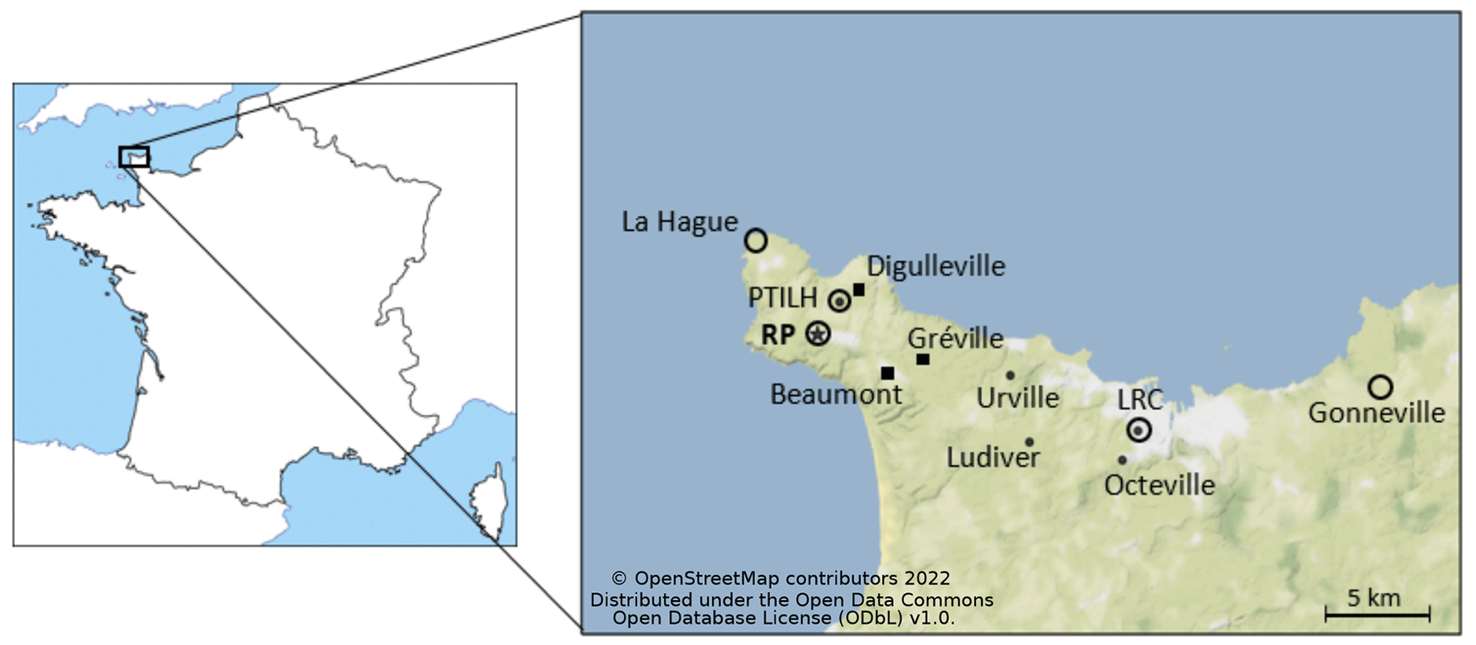
Figure 1 Location of North-Cotentin peninsula (left panel) and map of the monitoring sites (right panel). The dots and squares indicate the locations of the ⁸⁵Kr measurement stations carried out by IRSN and RP, respectively, as part of the DISKRYNOC campaign. The RP facility location is marked with a star. The circles indicate the locations of the 3D-wind measurement sites (from IRSN or Météo-France).

Past validation studies conducted in this framework have shown that dispersion simulation results are quite sensitive to the meteorological data used as input (Connan et al., 2013). The North-Cotentin peninsula of La Hague is a rocky area of approximately 15 km located at 190 m a.s.l. above cliffs, surrounded by the sea less than 5 km in most directions (Fig. 1). Such a complex terrain leads to spatially heterogeneous wind fields that may be difficult to accurately forecast. Therefore, this case study should provide good insights to examine the influence of meteorological uncertainties on atmospheric dispersion simulations.

2.2 Source term of ⁸⁵Kr

The La Hague RP has two production units called UP2-800 (1.87941^∘ W, 49.67705^∘ N) and UP3 (1.87606^∘ W, 49.67705^∘ N). Each of the two units has a stack for the discharge of ⁸⁵Kr with a height of 100 m and the two stacks are 200 m apart (Leroy et al., 2010).

During the reprocessing process of spent nuclear fuel, ⁸⁵Kr is intermittently released into the atmosphere from stacks of the plant during 30–45 min, separated by approximately 10 min intervals without releases. Depending on the industrial activity, long periods (a few hours to a few days or weeks) without releases are frequent. Both plants can operate separately and the release can come from one or both stacks. Release fluxes of ⁸⁵Kr (measured at a frequency of 10 min) were provided by the Orano RP for the study period. The radioactive concentration of the released ⁸⁵Kr depends on the burn-up of the reprocessed spent fuel and the processing rate of the plant (Connan et al., 2013).

The activity in ⁸⁵Kr released from the factory by the stacks (confidential data) is known with a time step of 10 min and an uncertainty of measurement in the order of 10 % in period of release (two channels of measurements for each stack). The discharge being intermittent, this 10 min time step ensures a precision that is indispensable for atmospheric dispersion studies. From 2019 to 2021, annual releases of the ⁸⁵Kr varied from 294 to 379 PBq yr⁻¹ (Orano, 2021).

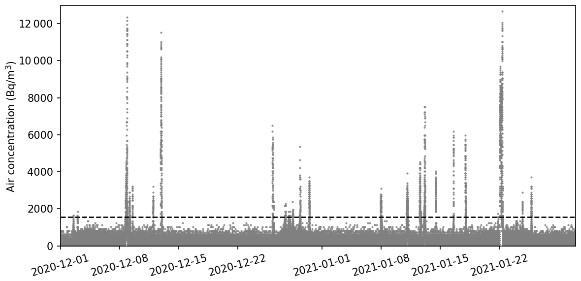
In this paper, the atmospheric dispersion of ⁸⁵Kr is studied along the continuous period of 2 months ranging from 1 December 2020 to 31 January 2021. This period comprises the detection of an important number of ⁸⁵Kr events at all measurement sites (Fig. 2) due to favorable wind direction.

Figure 2 ⁸⁵Kr air concentration measurements carried out at the LRC (Fig. 1) from 1 December 2020 to 31 January 2021. The horizontal dashed line shows the air concentration threshold (1545 Bq m⁻³) above which peaks are considered.

2.3 Measurements campaign of ⁸⁵Kr in the North-Cotentin province

The IRSN routinely monitors ⁸⁵Kr air concentrations close to the RP to not only study the transfer of radionuclides in the environment, but also validate the ADMs and improve the understanding of radionuclide dispersion in various atmospheric conditions (Maro et al., 2002, 2007; Leroy et al., 2010; Connan et al., 2014). Krypton-85 (⁸⁵Kr) is a very good tracer of atmospheric dispersion in short and medium distances since it is an inert gas (noble gas), it is not chemically or physically reactive, so it does not get depleted by rain (wet scavenging) or by dry deposition processes. In addition, ⁸⁵Kr has a sufficiently long half-life (${\mathit{\tau }}_{\mathrm{1}/\mathrm{2}}=\mathrm{10.7}$ years) for its radioactive decay to be negligible at short and medium distances.

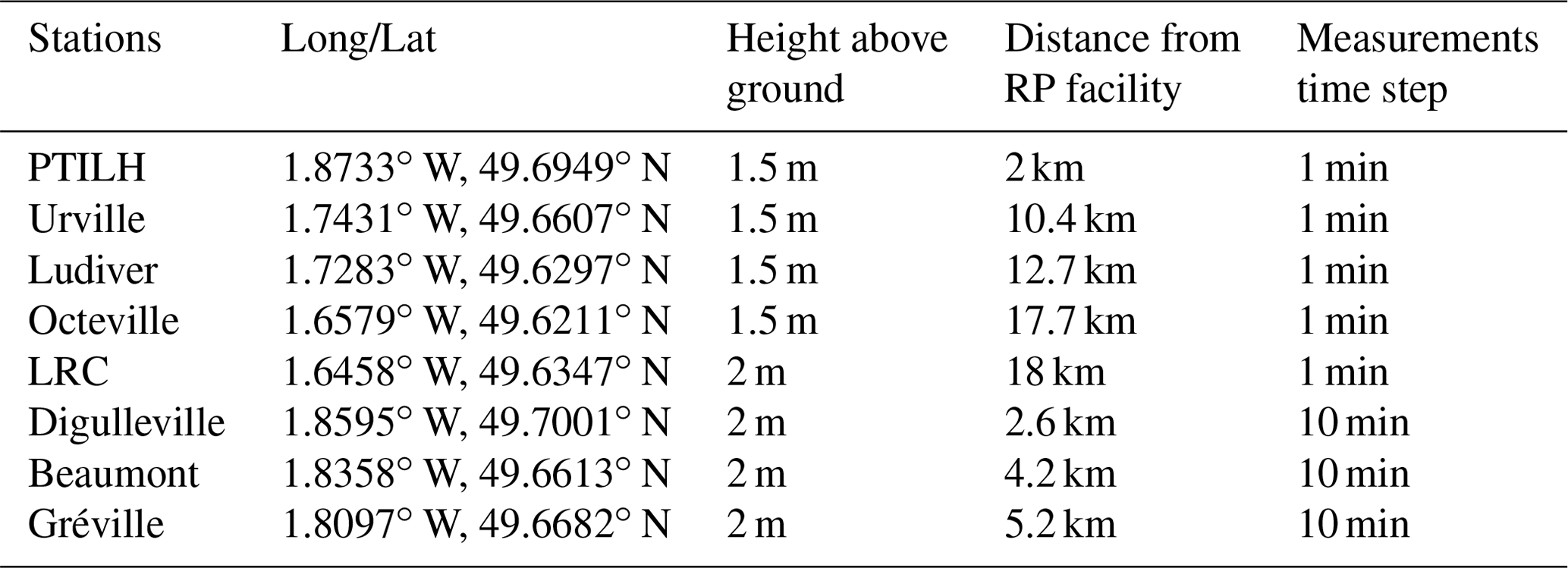
Since November 2020, IRSN has been carrying out a continuous ⁸⁵Kr air measurement campaign in several locations chosen at different distances and directions from the RP, as part of the DISKRYNOC project. This project aims to provide a comprehensive new observational dataset for model validation purposes. In this study, this dataset is used to acquire feedback on the use of meteorological ensembles to quantify the associated uncertainties. The eight closest air sampling locations from the RP used in this article, described in Table 1 and shown in Fig. 1, are as follows: PTILH (Instrumented Technical Platform of La Hague), Urville, Ludiver, Octeville, LRC, Digulleville, Beaumont, and Gréville. The IRSN is the owner of the first five stations, while the last three are Orano stations. The measurements have been carried out since mid-November 2020 and are expected to extend over approximately 18 months. This extended time period should provide a significant number of observations at all measurement sites. It should compensate for periods without reprocessing activity or with a wind direction towards the sea. Typical values of ⁸⁵Kr air concentrations in these stations range from tens to thousands Bq m⁻³ (depending on the distance from the RP, wind direction, plant reprocessing activities and atmospheric conditions). Continuous measurements are being performed every minute in the IRSN stations and every 10 min in the RP stations.

Table 1 Description of the 8 localizations of ⁸⁵Kr air concentration measurement stations used in this article.

The activity concentration in the air is determined by β counting in a Berthold LB123 or LB134 gas-filled proportional counter calibrated with a specially fabricated common ⁸⁵Kr source (Gurriaran et al., 2001). This method is only useful in near fields (less than 30 km) where the ⁸⁵Kr air concentration is sufficiently high. The same method has been used by Connan et al. (2014) and it has been documented by Gurriaran et al. (2004).

2.4 3D wind observations

Evidence from past studies has shown that (in the absence of deposition) 3D wind field is one of the most sensitive meteorological parameters for ADMs (Girard et al., 2014). For this reason, the performance of the AROME-EPS forecasts in terms of wind speed and direction should be assessed before they may be used for atmospheric dispersion. For this purpose, four kinds of observation data of wind have been used:

• The real-time ground observation acquisition network of Météo-France called RADOME, which has about 550 automatic ground observation stations spread over the whole French territory, among which two stations are located in the study area and are shown in Fig. 1: La Hague (1.9398^∘ W, 49.7251^∘  N) located ∼ 2.5 km from the RP plant, and Gonneville (1.4635^∘ W, 49.6526^∘ N) located ∼ 31 km from the RP plant. These stations provide continuous hourly measurement data of 10 m wind, temperature, humidity, rainfall, and surface solar radiation fields.

• Vertical wind profile measured by Doppler lidars (LIght Detection And Ranging). Atmospheric lidars are currently used for atmospheric measurements of aerosols and wind, and thus allow for climate monitoring, air quality, or cloud monitoring (Werner, 2005; Wu et al., 2022). A Doppler lidar (version Leosphere Windcube 2) was recently installed by the IRSN's LRC, on the PTILH measurement site, located ∼ 2 km from the RP plant (Table 1). This lidar provides wind data (speed and direction) at 10 min intervals on 13 vertical levels: 40, 60, 80, 100, 120, 140, 160, 180, 200, 220, 240, 260, and 280 m.

• Ultrasonic measurements acquired by Sodar (Sonic Detection And Ranging), which is a remote-sensing instrument often used in meteorology for the 3D acquisition of wind fields (speed and direction) on several vertical levels, using the Doppler effect on sound-wave levels (Tamura et al., 2001).
  The Sodar measurements used in this work come from the instrument located ∼ 200 m west (1.8901^∘ W, 49.6800^∘ N) of the RP facility, which provides measurements on 6 vertical levels: 0, 10, 50, 100, 150, and 200 m.

• Ultrasonic measurements by the LRC's anemometer (1.6458^∘ W, 49.6347^∘ N) installed at a height of 13 m above the ground. This instrument provides 10 min wind measurements.

Thus, five wind measurement points are available and used to evaluate the AROME-EPS meteorological ensemble over the two-month period of this work. This validation process has been done near the surface and on several vertical levels of the atmospheric boundary layer (ABL) since the knowledge of the evolution of the meteorological fields throughout the lower atmosphere with a good accuracy is beneficial for a short-distance ADM to describe the physical processes (e.g., turbulence) occurring in the ABL.

2.5 Description of AROME and AROME-EPS

The Météo-France NWP model, AROME, used in this study is summarized in Table 2 and extensively documented in Seity et al. (2011). AROME is a non-hydrostatic kilometer-scale NWP-limited area model. This model covers a geographical domain of about 1000 × 1000 km, centered over the French territory with 90 vertical levels and a horizontal resolution of 1.3 km. The lateral and upper boundary conditions are provided by the operational global NWP model ARPEGE (Courtier et al., 1991) of Météo-France. AROME runs 4 times per day, up to at least a 42 h range, starting from the initial times 00:00, 06:00, 12:00, and 18:00 UTC. Its 3D-Var data-assimilation scheme (Brousseau et al., 2011) is a state-of-the-art assimilation algorithm that produces analyses at 1.3 km resolution by correcting the model state at hourly time steps using different kinds of meteorological observations (in situ ground-based measurements, radar reflectivities and winds, satellite radiances, among others).

Table 2 Description of AROME and AROME-EPS.

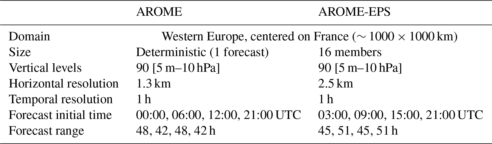
The AROME-EPS (Bouttier et al., 2016) model used in this article is a 16-member ensemble based on the AROME model at 2.5 km (Table 2). The ensemble runs 4 time per day, up to at least a 45 h range, at 03:00, 09:00, 15:00, and 21:00 UTC. The 16 AROME-EPS perturbed initial conditions are built from the AROME 3D-Var analyses on which perturbations from the ensemble data assimilation (EDA) at 3.25 km resolution are added (Raynaud and Bouttier, 2016). The AROME-EDA comprises 25 members that are obtained by perturbing the observations and the model state during the assimilation process. The outputs from both are combined and interpolated to 2.5 km to produce the initial conditions of the AROME-EPS. The lateral and upper boundary conditions (Bouttier and Raynaud, 2018) are provided by the Météo-France ARPEGE-EPS operational global EPS (Descamps et al., 2015).

Besides the initial errors, forecast uncertainty also arises from the dynamic part of the model (e.g., spatial and temporal discretization of the equations that represent phenomena whose characteristic scale is larger than the mesh size), or from the physical part of the model (e.g., corrective terms added to the dynamic equations to take into account the effect of phenomena whose scale is smaller than the mesh size). To account for model uncertainties in the AROME-EPS forecasts, the stochastically perturbed parametrization tendencies (SPPT) scheme is used (Palmer et al., 2009; Bouttier et al., 2012). This method consists of adding random perturbations to the physics tendencies in models.

2.6 Description of the pX model

The IRSN's Gaussian puff model, pX, used in this work is part of the operational platform C3X (Tombette et al., 2014), which is used by IRSN Emergency Response Center in case of an accidental radioactive release. The pX model is used to simulate the atmospheric dispersion of radionuclides on short and medium distances (500 m–50 km) (Korsakissok et al., 2013; Mathieu et al., 2012). The principle of such a dispersion model is based on the following assumptions:

• The release comes from a point source.

• A continuous release can be discretized into a series of puffs transporting a given amount of pollutants.

• Within each puff, the meteorological variables can be considered homogeneous.

• The concentration of pollutant in the puff can be represented by a Gaussian law in each of the three directions (Appendix B).

For an instantaneous release of a mass Q of a given radionuclide, the concentration c at a given point $(x,y,z)$ and a time t is given by the following:

$$\begin{array}{}\text{(1)}& \begin{array}{rl}& c(x,y,z,t)={\displaystyle \frac{Q}{{\left(\mathrm{2}\mathit{\pi }\right)}^{\mathrm{2}/\mathrm{3}}{\mathit{\sigma }}_x{\mathit{\sigma }}_y{\mathit{\sigma }}_z}}\times \\ & \exp \left[-{\displaystyle \frac{\mathrm{1}}{\mathrm{2}}}\left({\displaystyle \frac{(x-x_{\mathrm{0}}{)}^{\mathrm{2}}}{{\mathit{\sigma }}_x^{\mathrm{2}}}}+{\displaystyle \frac{(y-y_{\mathrm{0}}{)}^{\mathrm{2}}}{{\mathit{\sigma }}_y^{\mathrm{2}}}}+{\displaystyle \frac{(z-z_{\mathrm{0}}{)}^{\mathrm{2}}}{{\mathit{\sigma }}_z^{\mathrm{2}}}}\right)\right],\end{array}\end{array}$$

where σ_x, σ_y, and σ_z are the Gaussian standard deviations of the diffusion of the puffs over time in the three directions of space and $(x_{\mathrm{0}},y_{\mathrm{0}},z_{\mathrm{0}})$ is the position of the mass center of the puff, which is transported by the mean wind flow. If x is the mean wind direction, and U is the mean wind speed in the x direction, then the position of the center of the puff at each time t+dt from its position at time t is

$$\begin{array}{}\text{(2)}& {\mathit{x}}_{\mathbf{0}}(t+\mathrm{\Delta }t)={\mathit{x}}_{\mathbf{0}}\left(t\right)+\mathit{U}\left(t\right)\mathrm{\Delta }t.\end{array}$$

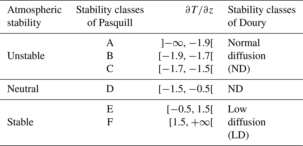
This advection scheme allows the transportation of the puffs' mass centers through a non-stationary and heterogeneous wind field. In addition, the puffs are growing over time to represent the plume's mixing by atmospheric turbulence. This is represented in Eq. (1) by the standard deviation σ_x, σ_y, and σ_z that increase over time. This increase of plume spread depends on the atmospheric stability and is described by empirical standard deviation laws. In the pX model, the laws of Doury (Doury, 1976) or Pasquill (Pasquill, 1961) can be used. In this work, Pasquill stability was determined using two methods: (i) Pasquill–Turner (Turner, 1969) and (ii) the temperature gradient between 10 and 100 m in the meteorological forecasts (Seinfeld and Pandis, 1998), i.e., three stability diagnoses which are compared in this work (Appendix A1).

For a continuous emission of release rate q_s (in Bq s⁻¹) that is discretized into a series of N puffs, each puff i containing a mass Q_i=q_sΔt, the concentration c at a given point is computed as the sum of the contribution of all puffs:

$$\begin{array}{}\text{(3)}& c(x,y,z,t)=\sum _{i=\mathrm{1}}^N{c}_i(x,y,z,t),\end{array}$$

where c_i is given by Eq. (1).

Finally, the mass of the material transported by the puff is depleted by wet and dry deposition as well as by radioactive decay. In our case, the transported mass will be assumed to remain constant over time, since ⁸⁵Kr is an inert gas (no deposition) with a long half-life (no radioactive decay at short distance) as shown previously. Equation (1) is also modified to take into account reflections on the ground and ABL height under certain conditions. Specifically, reflections on the ABL height are considered in unstable situations (when a capping inversion is assumed).

3 AROME-EPS verification

3.1 Scores for AROME-EPS verification

Before coupling the NWPs from AROME-EPS to the pX model, it is necessary to evaluate them in order to have an exhaustive overview of their quality and to take it into account in the interpretation of atmospheric dispersion simulations. For this purpose, two common scores, among others, used by the meteorological community for the evaluation of ensemble skill, have been calculated based on the observations of 3D-wind speed and direction described in Sect. 2.4:

•  

  Bias. In order to identify the systematic deviations of AROME-EPS meteorological ensemble forecasts from the observations, the bias over all days of the period of interest for a variable X is calculated at each forecast range t by the following equation:

  $$\begin{array}{}\text{(4)}& \mathrm{Bias}\left(t\right)={\displaystyle \frac{\mathrm{1}}{N_{\mathrm{day}}}}\sum _{d=\mathrm{1}}^{N_{\mathrm{day}}}\left(\langle X_{\mathrm{mod}}^{(t,d)}\rangle -X_{\mathrm{obs}}^{(t,d)}\right),\end{array}$$

  where N_day is the number of days of the interest period; $\langle X_{\mathrm{mod}}^{(t,d)}\rangle$ is the AROME-EPS ensemble mean at forecast range t on day d and $X_{\mathrm{obs}}^{(t,d)}$ is the observed value at the same instant.

•  

  Spread-skill. As shown by Fortin et al. (2014), the ability of an ensemble to represent simulation errors can be evaluated by comparing, at each forecast range, the skill (or root mean square error, RMSE) of the ensemble mean and its spread (Spd), the latter calculated relative to the ensemble mean (Raynaud et al., 2012; Charrois et al., 2016). For a variable X, the ensemble Spd and RMSE terms are defined, at each forecast range t, as follows:

  $$\begin{array}{}\text{(5)}& {\displaystyle }\mathrm{Spd}\left(t\right)=\sqrt{{\displaystyle \frac{\mathrm{1}}{N_{\mathrm{day}}}}\sum _{d=\mathrm{1}}^{N_{\mathrm{day}}}{\displaystyle \frac{\mathrm{1}}{N_{\mathrm{ens}}-\mathrm{1}}}\sum _{n=\mathrm{1}}^{N_{\mathrm{ens}}}{\left(X_{\mathrm{mod},n}^{(t,d)}-\langle X_{\mathrm{mod}}^{(t,d)}\rangle \right)}^{\mathrm{2}}},\text{(6)}& {\displaystyle }\mathrm{RMSE}\left(t\right)=\sqrt{{\displaystyle \frac{\mathrm{1}}{N_{\mathrm{day}}}}\sum _{d=\mathrm{1}}^{N_{\mathrm{day}}}{\left(\langle X_{\mathrm{mod}}^{(t,d)}\rangle -X_{\mathrm{obs}}^{(t,d)}\right)}^{\mathrm{2}}},\end{array}$$

  where N_ens represents the ensemble size (N_ens=16 in the case of AROME-EPS). The value of variable X given by the ensemble member n at the forecast range t is $X_{\mathrm{mod},n}^{(t,d)}$. This diagnostic can be summarized by calculating the spread–skill ratio, which should be as close to 1 as possible. Values less than 1 (respectively greater than 1) indicate that the ensemble is underdispersive (respectively overdispersive).

3.2 Model-to-data comparison of AROME-EPS

The evaluation of the quality of AROME-EPS predictions was carried out over the two-month period considered in this study (December 2020–January 2021). This evaluation process is done independently for each of the 03:00, 09:00, 15:00, and 21:00 UTC forecasts for all stations described in Sect. 2.4. The results for all forecasts and stations are similar. Therefore, only the results of the 15:00 UTC forecast are shown here for two configurations: (i) at 10 m height (two RADOME stations: La Hague and Gonneville) and (ii) at several levels of ABL for stations where vertical wind profile measurements are available (lidar at PTILH and Sodar at the RP site).

Figure 3 shows the ensemble biases in terms of 10 m wind speed and direction aggregated from La Hague and Gonneville stations. In the case of wind speed, the ensemble mean is above the observation for most of the forecast ranges, resulting in a slight systematic bias which varies between 0.71 and 1.45 m s⁻¹. The evolution of both the forecasts and observations (and eventually the resulting bias) shows a marked diurnal cycle. The maximum bias is around 15:00 UTC, corresponding to the forecast range of 25 h, with approximately no bias in the first forecast range. For the wind direction, there is a good average performance of the model as shown by the good agreement between the averages of the forecasts and observations. The mean bias of the model oscillates around zero, with maximum and minimum values of +7.8 and −13.3^∘, respectively.

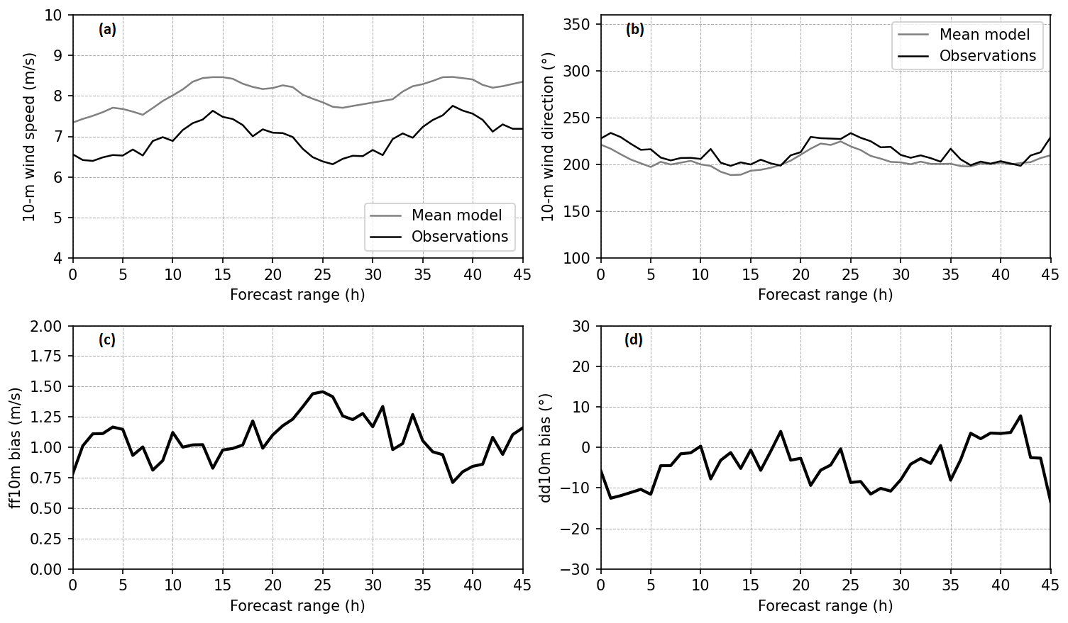
Figure 3 Ensemble mean and observations (a, b) as a function of forecast range, and the resulting bias (c, d) for both 10 m wind speed (referred to as ff10m) and direction (referred to as dd10m), aggregated from the two ground measurement stations: La Hague and Gonneville.

Figure 4 shows the ensemble spread and skill evolution over the forecast range. For wind speed, the spread of the ensemble is consistent with the RMSE with respect to the observations, with a slight underdispersion, while for wind direction, the ensemble spread is above the RMSE at all forecast ranges. This overdispersion in terms of wind direction should be kept in mind when interpreting the ensemble atmospheric dispersion simulations.

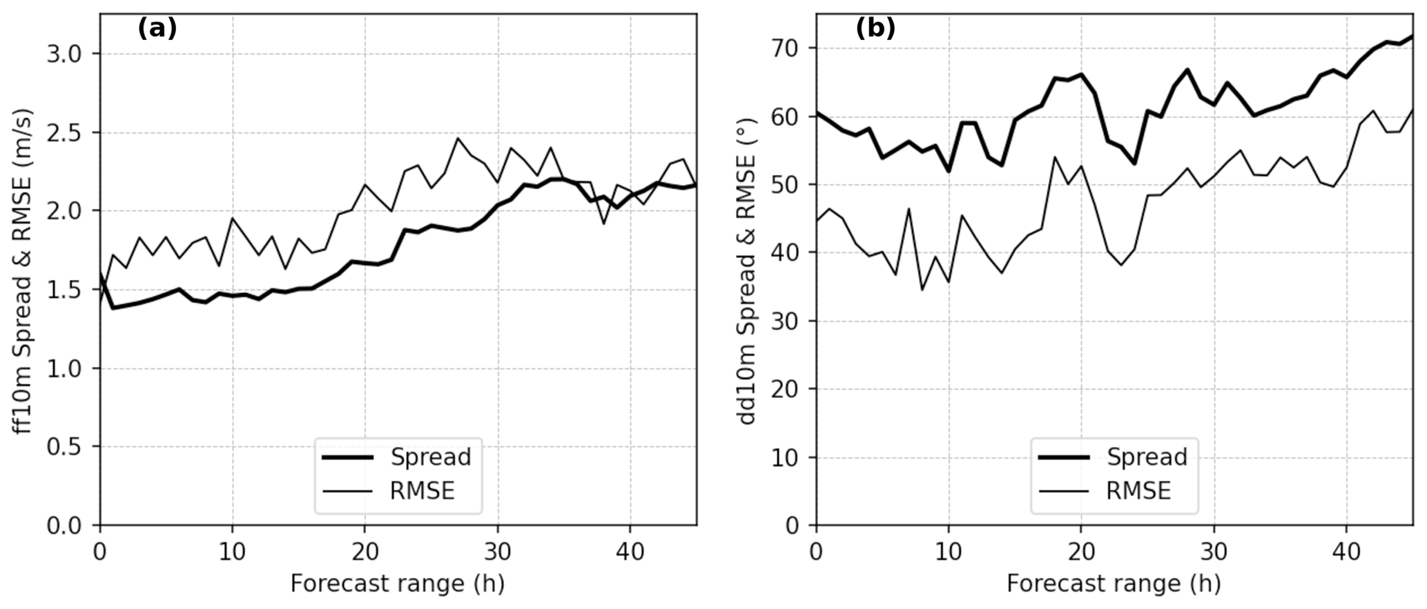
Figure 4 Ensemble spread and RMSE of the ensemble mean forecast for both 10 m wind speed (referred to as ff10m) (a) and direction (referred to as dd10m) (b) aggregated from the two ground measurement stations: La Hague and Gonneville, as a function of the forecast range.

To complement this evaluation at 10 m height, it is worth examining the quality of the AROME-EPS meteorological ensembles at different vertical levels in the lower atmosphere. To do so, the bias and the spread–skill ratio have been calculated at several vertical levels above ground. The results at the PTILH station are presented in Fig. 5 and summarized in Table 3. The wind speed forecasts are slightly less biased and overdispersive at higher altitudes than at lower ones, with an overdispersion more pronounced in the earlier forecast ranges. The latter is probably due to an imperfect accounting of modeling and/or initial condition uncertainties in the perturbation process. However, the bias at 40 m (lidar measurements) and 10 m (in situ measurements) are consistent, which means that the high bias in the lower layers is probably not due to lidar measurement errors. It may be due to the representation of surface processes in AROME in this area which is characterized by a complex orography and heterogeneous surfaces (sea and land). For the wind direction, there is no significant dependency of biases and spread of the ensembles with respect to the altitudes.

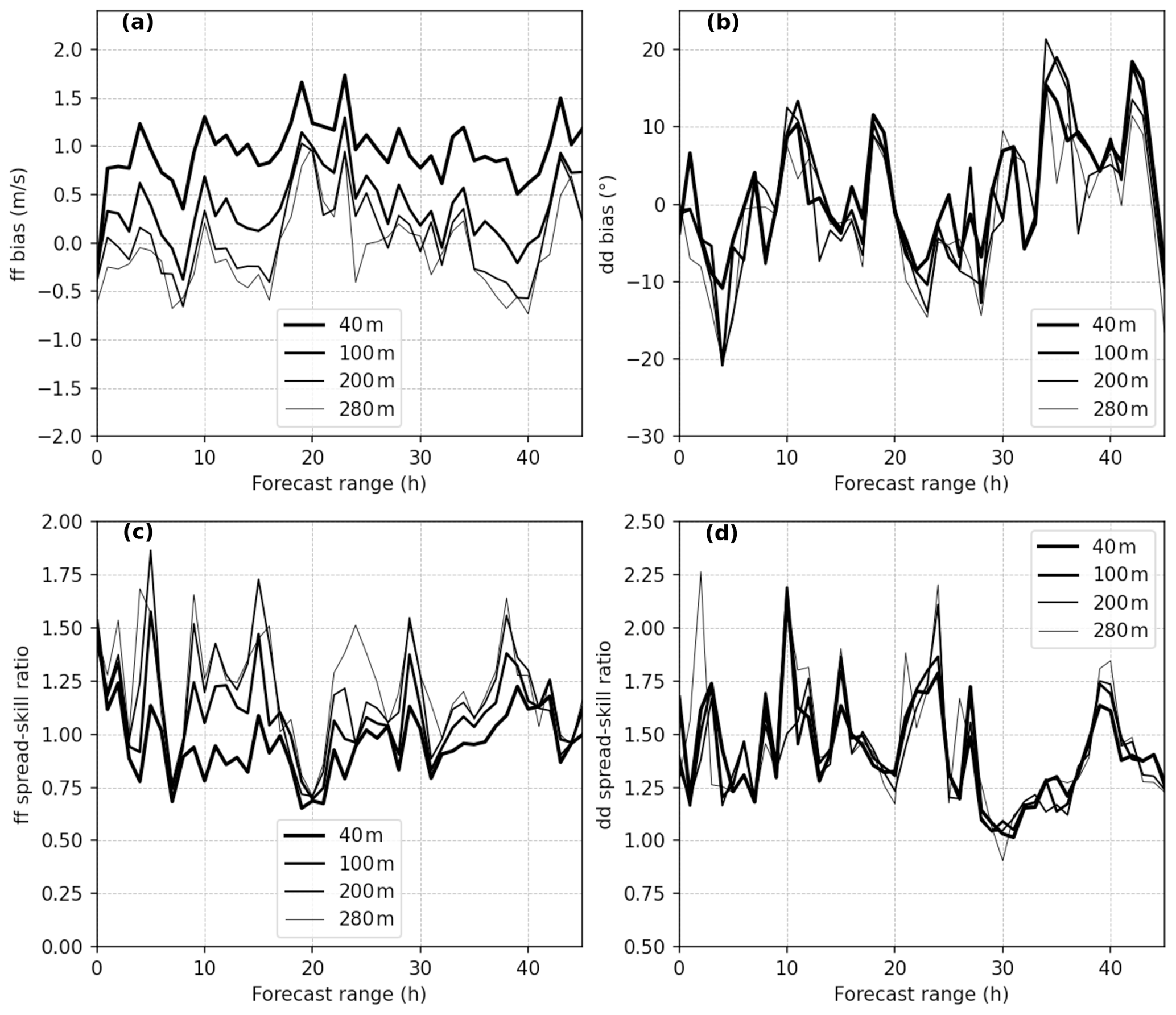
Figure 5 Bias (a, b) and spread–skill ratio (c, d) of the ensemble between 40 and 280 m above ground, for both wind speed (referred to as ff) (a, c) and direction (referred to as dd) (b, d) measured by lidar at the PTILH station, as a function of forecast range.

To summarize, the assessment of the consistency of AROME-EPS forecasts showed that they perform well by comparison to wind speed and direction measurements in the North-Cotentin area for the selected period, despite slight errors in the wind speed forecast. The same conclusion was reached for deterministic AROME forecasts (not shown here), by calculating the bias from wind observations.

4 Analysis of the ensemble dispersion simulations

4.1 Coupling AROME-EPS and pX model

Once meteorological forecasts from AROME-EPS have been qualified as shown in Sect. 3, they are coupled to the Gaussian dispersion model pX (Sect. 2.6). This process consists of running several simulations in parallel with the pX model, each using a different member of the AROME-EPS ensemble as input, along with the source term data provided by the RP La Hague. This allows the generation of an ensemble of dispersion simulations composed of 16 members (hereafter called the pX ensemble). Furthermore, in order to quantify the benefit of using ensembles instead of deterministic simulations, an additional pX simulation was performed using the deterministic weather forecast from AROME as input of the model. This simulation is called deterministic pX in the following section.

4.1.1 Temporal continuity of AROME-EPS members

In the case of accidental releases that span a long time period, it is important to properly build continuous time series from several forecasts made at different initial times, without causing brutal jumps in spread between forecasts from 2 consecutive days. Besides, fine-scale weather forecasts are, usually, not available until a few hours after their start. To deal with this issue, this study proposes using the closest available forecast at the beginning of a day. In other words, to simulate a release occurring from 00:00 to 23:00 h of a day D, the AROME-EPS forecasts starting from 15:00 UTC of the day before (D−1) are used. Thus, the first 8 forecast hours are skipped and the next 24 h [09:00–32:00 h] are used to cover the entire day. In the same way, the forecast starting from 15:00 UTC of day D is used to cover the day D+1. Figure 6 illustrates this cycle. Then, these intervals are combined to cover the three simulation periods detailed in Table 5, by connecting each member i of day D with member i of day D+1.

Note that to perform pX deterministic simulations, the deterministic weather forecasts from AROME are built in the same way, by using the forecast starting from 12:00 UTC. In this case, the first 11 forecast hours were skipped and the next 24 h were used [12:00–35:00 h].

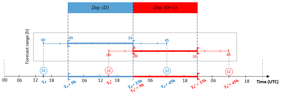
Figure 6 Illustration of meteorological forecasts used from AROME-EPS (in bold) as input to pX: the forecast starting from 15:00 UTC on a day D is used to cover the next day D+1.

4.1.2 pX simulation setup

The calculation domain of pX is defined by the grid of meteorological forecasts, and the puffs that leave this domain no longer participate in the concentration calculations. Moreover, the concentration calculated on a point located on the border of the meteorological domain will only account for the contribution of the puffs inside. It is, therefore, necessary to define a simulation domain whose borders are sufficiently far from the calculation points (i.e., ⁸⁵Kr measurements sites in Fig. 1). Thus, a 60 × 60 km domain centered on the source (i.e., RP) was defined, where the meteorological forecasts were interpolated on a Cartesian grid with 2.5 km of horizontal resolution, leading to a horizontal mesh of 24 × 24 cells. This process was accomplished by a weather pre-processor that was developed as part of this study.

Considering the objectives of this work, only the first 25 vertical levels outputs from AROME (10–3000 m) are used here to cover the entire ABL. The ABL height is diagnosed from AROME forecasts as the lowest altitude where the turbulent kinetic energy is below 0.01 m² s⁻². As a result, it may happen that this diagnostic reaches unrealistically low values, as low as 10 m. In order to avoid such low values and to ensure that the source emission does not occur above the ABL, a minimum value of 200 m is imposed to the ABL height before being applied to the pX simulations.

Table 3 The AROME-EPS ensemble bias and spread–skill ratio averaged over forecast range in the vertical levels observed by lidar located in the PTILH site.

Even though the NWP forecasts are given with an hourly frequency, the pX simulations were performed in this study with a time step of 10 min in order to better capture the temporal variations of the plume. Sensitivity tests showed that the pX simulations with the two Pasquill-based stability diagnoses (Pasquill–Turner and temperature gradient) gave very similar results with a slightly better performance of the diagnosis of temperature gradient. In the following section, simulations with Pasquill (called pX–Pasquill) standard deviations will thus be computed with the latter stability diagnosis and will be compared with simulations using Doury standard deviations (called pX–Doury).

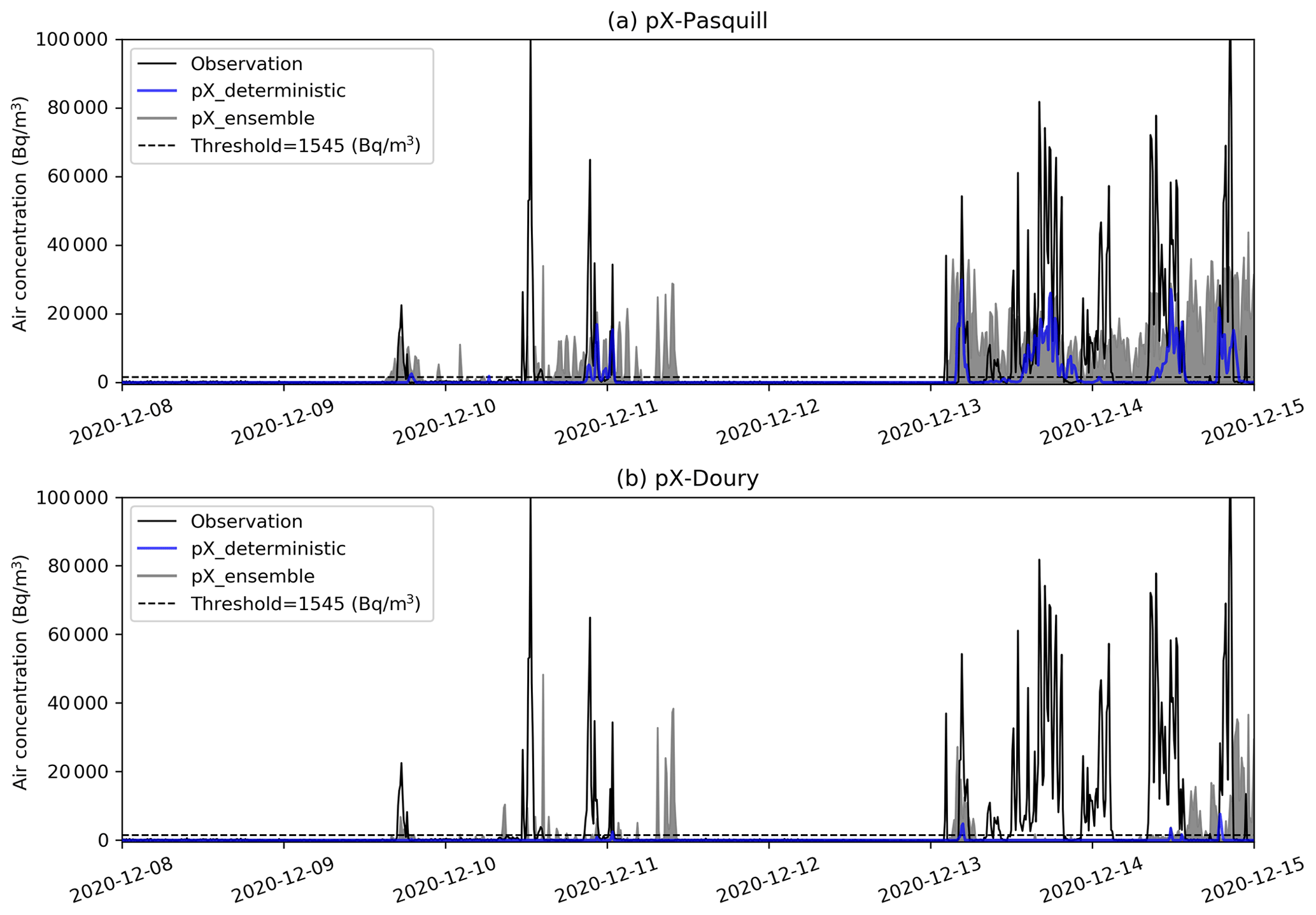
Figure 7 pX–Pasquill (a) and pX–Doury (b) ensemble and deterministic simulations of ⁸⁵Kr air concentration compared to the observation in the first aggregated period (Table 5), at the PTILH station. The horizontal dashed line shows the air concentration threshold (1545 Bq m⁻³) above which peaks are considered.

Figure 8 The same as in Fig. 7, but at the LRC station.

Finally, the effects of the complex topography (coastline, rocky terrain) and buildings on the plume dispersion may lead to downwash effects that are not explicitly taken into account by the Gaussian puff model. To compensate for this limitation, an effective height that differs from the physical stack height may be used as input. In this case, five values of effective height have been tested: 20, 50, 100, 150, and 200 m, and the most optimum simulations were obtained by using the physical stack height of 100 m.

4.2 Qualitative results and discussion

In this section, we illustrate the behavior of the dispersion simulations at two stations located at short and medium distances from the source. For this purpose, a short time period was selected where a few marked events occurred.

4.2.1 Comparison of ensemble and deterministic dispersion results

Figures 7 and 8 show an example of dispersion results at the PTILH (2 km from the source) and LRC stations (18 km from the source), respectively. There are observed peaks that the deterministic simulation does not reproduce while some ensemble members simulate them with acceptable accuracy. This highlights the potential interest of the ensemble approach compared to the deterministic one. In addition, a visual analysis of the results shows that the pX–Pasquill simulations correctly predict most peaks at the PTILH station (Fig. 7), although with a tendency to underestimate their maximum value. At the same station, pX–Doury simulations show a strong underestimation of concentrations, resulting in a failure to forecast most observed peaks. As the PTILH station is located only 2 km from the source, the release conditions (initial buoyancy and building downwash effects) largely influence the concentrations at this short distance.

In our simulations, the use of the stack height (100 m) as release height does not allow the accurate prediction of significant ground concentrations at this distance due to approximations made in the Gaussian model that does not include building downwash effects. This is especially the case when using Doury standard deviations, which simulate a very narrow plume on the vertical, resulting in an underestimation of ground concentrations in the case of elevated release. This phenomenon, that characterizes pX–Doury simulations in stable situations, was specifically shown in the case of the La Hague RP (Connan et al., 2014; Korsakissok et al., 2016). At the LRC station (Fig. 8), located farther from the source, this underestimation is much less visible and peaks are better reproduced. There are still, however, peaks that are missed by the deterministic simulations and forecast by some members of the ensemble. This can be explained by the meteorological uncertainties, as detailed in the following section.

4.2.2 Sensitivity to wind and atmospheric stability

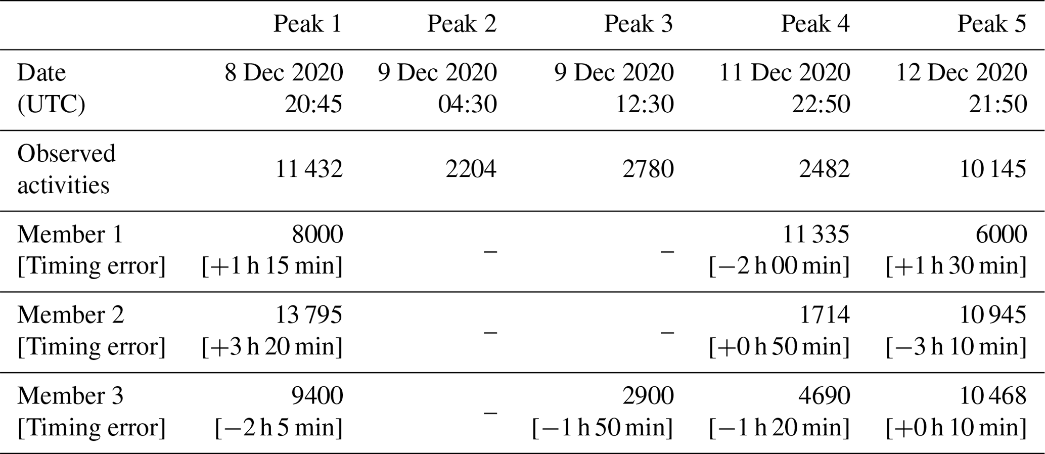
In this section, the sensitivity to meteorological variables such as wind and stability is detailed. The aim is to illustrate how small variations in these parameters affect the outputs of atmospheric dispersion simulations. For this purpose, three members of the pX–Pasquill ensemble which have different behaviors are shown. The study is carried out at the LRC station, where both air concentration and wind measurements are available. This station is representative of the model behavior at medium distance, where release conditions are of relatively less importance than meteorological uncertainties. Table 4 summarizes the five observed peaks (with peaks 2, 3, and 4 being much smaller than peaks 1 and 5) from 8 December 2020 to 12 December 2020, when the ensemble behavior is studied.

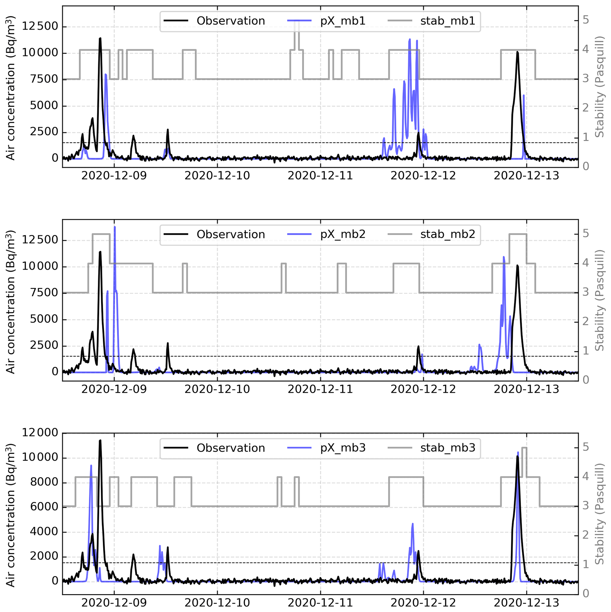
Figure 9 The three selected pX ensemble members (referred to as pX_mb1, pX_mb2, and pX_mb3) of ⁸⁵Kr activities, at the LRC site, from 8 December 2020 at 12:00 UTC to 13 December 2020 at 12:00 UTC. The gray curves represents the hourly Pasquill stability classes (referred to as stab_mb1, stab_mb2, and stab_mb3) used to generate each of the three pX members. The horizontal dashed line shows the air concentration threshold (1545 Bq m⁻³) above which peaks are considered.

Table 4 The five observed peaks of ⁸⁵Kr at the LRC station (Fig. 9) from 8 to 12 December 2020, and the simulated peaks in the three selected members (in Bq m⁻³), for pX–Pasquill configuration.

Although the wind forecasts used to generate the three pX simulations in Fig. 9 are sufficiently close to the observation at the LRC station around the time of peak occurrences (as shown in Fig. 10), some events are reproduced either with small errors in timing (i.e., delay/advance of 2–3 h) or with errors in intensity (i.e., underestimation/overestimation). This can be a result of local effects on the dispersion simulations. In other words, when one is interested in calculating the activity concentration at a point in space, a small error in the wind speed and/or direction can have a significant impact on the estimation of the peaks timing and intensity, due to the sharp concentration gradient. Figure 11 illustrates this issue in the case of peak 3 of member 1 in Fig. 9 and Table 4. This peak underestimates the air concentration because it is located close to the edge of the plume where the concentration gradients are expected to be high.

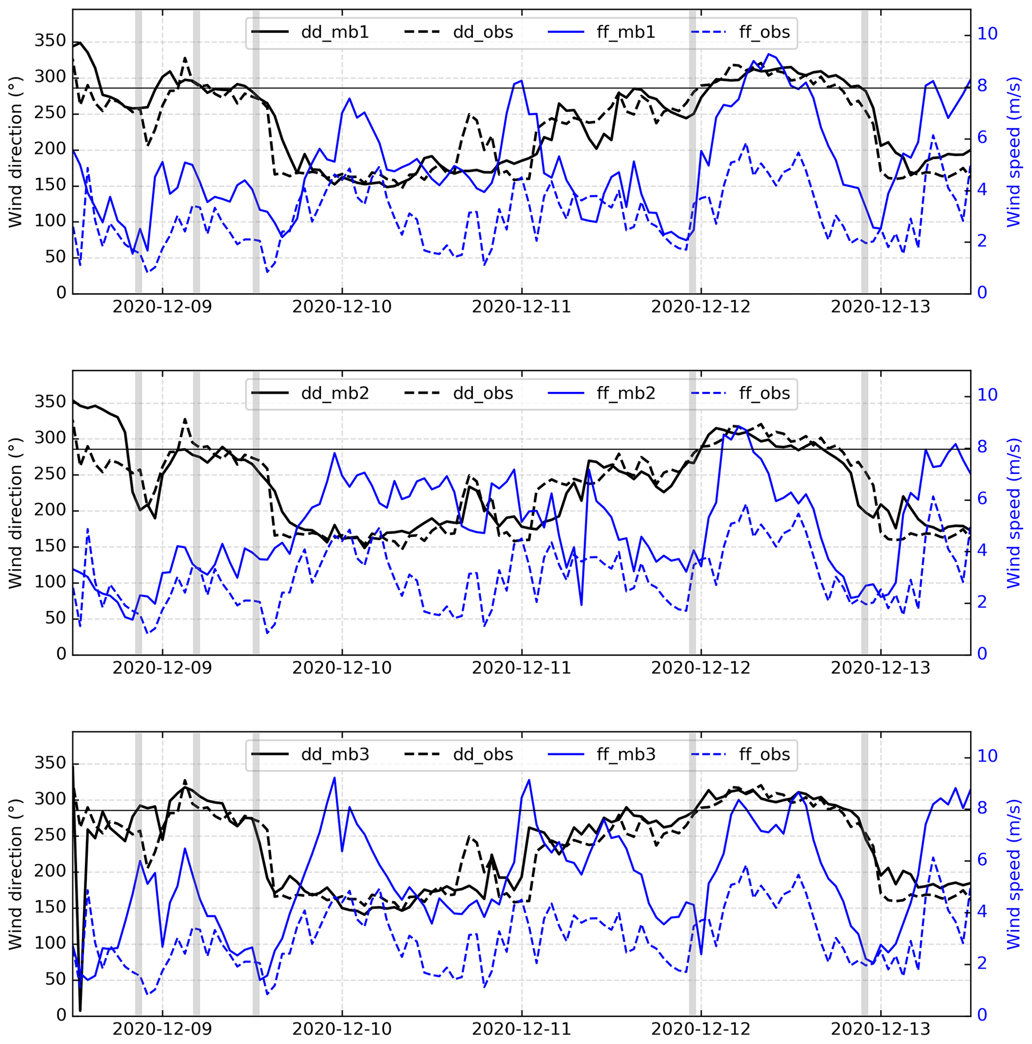
Figure 10 The three wind forecasts from AROME-EPS (solid curves) used to generate the pX simulations presented in Fig. 9, compared to wind observations stored at LRC (dashed curves); ff and dd denote, respectively, wind speed and direction, while mb1, mb2, and mb3 denote each of the three AROME-EPS members. The vertical gray lines shows the occurrence time of the five peaks presented in Table 4. The horizontal line shows the angle of the LRC station with respect to the source (286^∘), which corresponds to the wind direction that transports the plume from the source to LRC.

Figure 11 Simulation of the dispersion of the ⁸⁵Kr exceeding 1545 Bq m⁻³ in the case of member 1 presented in Fig. 9 and Table 4, surrounding the moment of the observed peak 3 at the LRC station.

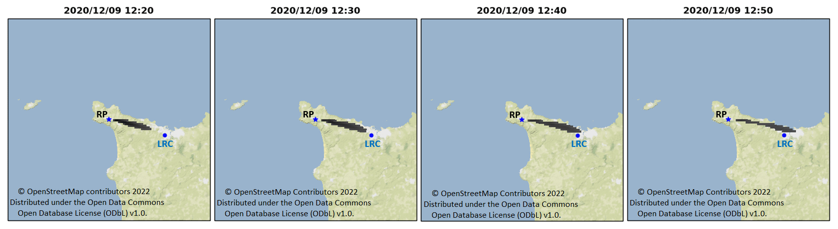
Figure 9 also shows the effect of the diagnosed stability classes on the dispersion simulations. Almost all the simulated peaks are associated with stable conditions of the atmosphere (4th or 5th Pasquill stability class, corresponding to classes E and F, respectively, in Appendix A1). This may explain the failure of members 1 and 2 to reproduce the observed peak 3 which is associated with neutral stability conditions (3rd stability class, corresponding to class D of Pasquill).

In order to better understand the effect of the stability conditions on the pX simulations, a test was carried out by using stationary stability classes in the simulations, each time using one of the three classes obtained by the temperature gradient diagnosis in the period shown in Fig. 9. The result, shown in Fig. 12, confirms that the diagnosed stability classes have a significant effect, mainly on the simulated intensity. It allows an explanation of some model failures, such as the peak 3 for the member 1, but not others. In most cases, the 4th stability class gives the highest ⁸⁵Kr concentration.

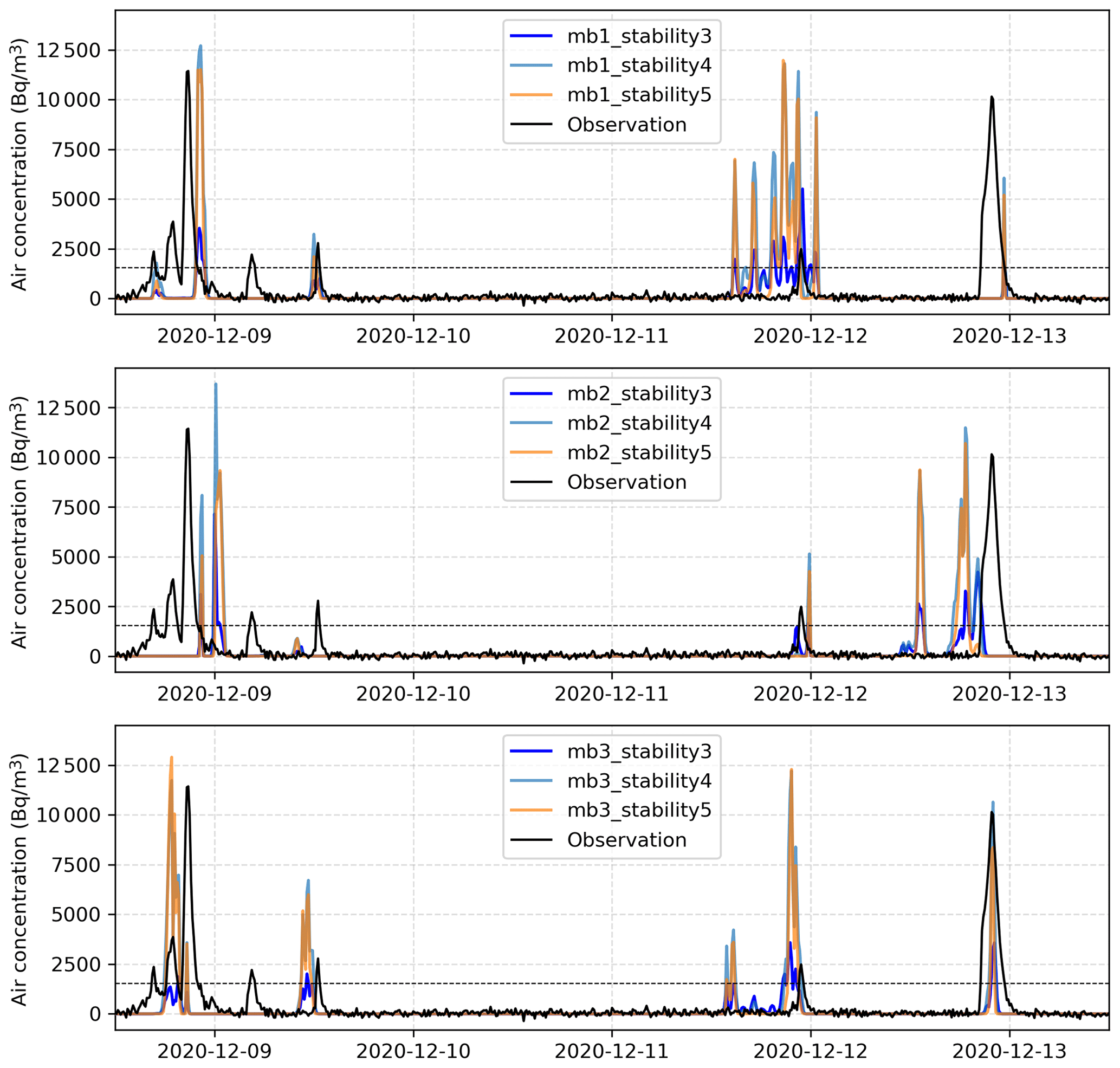
Figure 12 The same experiments as in Fig. 9, but with three stationary stability classes of Pasquill: 3rd, 4th, and 5th class; mb1, mb2, and mb3 denote, respectively, each of the three members of pX ensemble simulations.

In summary, while some detections/non-detections can be easily explained by examining wind speed and direction time series, other features are less predictable on this sole basis, due to the interaction between the variables and the possible accumulation of small direction errors over the plume trajectory.

4.3 Statistical evaluation of the dispersion ensemble

4.3.1 Evaluation procedures

It is often a desirable feature for a dispersion model to be able to correctly predict a threshold exceedance. It is particularly useful for decision-making purposes, when protective actions for the population are based on the prediction of zones where a given dose threshold could be exceeded. Evaluating the model performance for this kind of purpose is often based on contingency tables (Wilks, 2019) that allow the comparison of the series of observations and simulations by counting four features: (i) true positive (TP) – when a peak is observed and well simulated, (ii) false negative (FN) – when a peak is observed but not simulated, (iii) false positive (FP) – when there is no observed but simulated peak, and (iv) true negative (TN) – when there is no observed and no simulated peak.

The method used by Quérel et al. (2022) is based on this principle and used to evaluate a series of peaks from deterministic simulation against observations. This method consists of evaluating the success/failure of the model for each observed or simulated peak, including a defined temporal tolerance. However, in the case of an ensemble, the same procedure cannot apply because there are multiple simulations and so unobserved events cannot be well-defined. In addition, it often occurs that the FPs from different members constitute a series that exceeds the correlation timescale between peaks (i.e., the temporal offset between two peaks at which they no longer correspond to the same event). Hence, one cannot decide whether all these TPs correspond to the same event or several. To deal with this problem, the method used in this work comprises the discretization of the time series by sliding intervals of length Δt and moving time τ (Fig. 13). For the kth discretization step, the evaluation interval is (t^′, $t^{\prime }+\mathrm{\Delta }t$), such that

$$\begin{array}{}\text{(7)}& t^{\prime }=t_{\mathrm{0}}+(k-\mathrm{1})\mathit{\tau },\end{array}$$

where t₀ is the initial time of the time series.

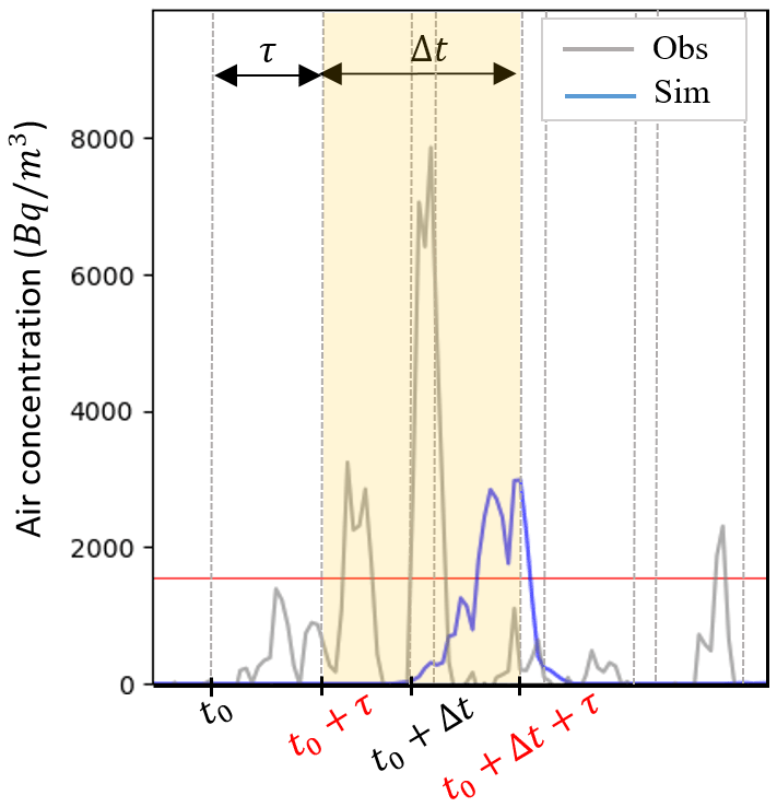
Figure 13 Illustration of the temporal discretization method by sliding intervals used in this study. This figure shows the case of the second time interval of length Δt: ($t_{\mathrm{0}}+\mathit{\tau },t_{\mathrm{0}}+\mathrm{\Delta }t+\mathit{\tau }$).

Then, the maximum values from each ensemble simulation are compared to the maximum observed value in each discretization interval. Thus, considering a threshold of 1545 Bq m⁻³ (corresponding to the detection threshold for air concentration of ⁸⁵Kr) and a given decision threshold x (i.e., the number of members at which the success/failure of the ensemble is considered), the four features of the contingency tables are defined in this case as follows:

• TP: when a peak is observed and well simulated by at least x members,

• FN: when a peak is observed but simulated by a number of members less than x,

• FP: when there is no observed peak but simulated by at least x members,

• TN: when there is no observed peak but simulated by a number of members less than x.

This method also allows a decrease in the number of TN without having a statistically significant impact on the scores thanks to the normalization in the contingency tables. This advantage gives the possibility of using scores that integrate the number of TN, contrary to the classical method which is not adapted to the case of rare events (i.e., the case of non-continuous events in time).

Then, the performance of the ensemble is measured using hit rate (H) and false alarm rate (F) metrics (Quérel et al., 2022; Wilks, 2019). The hit rate (also called recall) is the fraction of the observed events that are successfully reproduced (Eq. 8). The false alarm rate is the fraction of the simulated peaks that are not observed (Eq. 9).

$$\begin{array}{}\text{(8)}& {\displaystyle }H={\displaystyle \frac{\mathrm{TP}}{\mathrm{TP}+\mathrm{FN}}},\text{(9)}& {\displaystyle }F={\displaystyle \frac{\mathrm{FP}}{\mathrm{FP}+\mathrm{TN}}}.\end{array}$$

To choose the most representative combination (Δt,τ), we consider that two events are independent if they are more than 3 h apart. Thus, six combinations (Δt,τ) are tested by the statistical scores below: $(\mathrm{\Delta }t=\mathrm{1}h,\mathit{\tau }=\mathrm{1}h)$, $(\mathrm{\Delta }t=\mathrm{2}h,\mathit{\tau }=\mathrm{1}h)$, $(\mathrm{\Delta }t=\mathrm{2}h,\mathit{\tau }=\mathrm{2}h)$, $(\mathrm{\Delta }t=\mathrm{3}h,\mathit{\tau }=\mathrm{1}h)$, $(\mathrm{\Delta }t=\mathrm{3}h,\mathit{\tau }=\mathrm{2}h)$, and $(\mathrm{\Delta }t=\mathrm{3}h,\mathit{\tau }=\mathrm{3}h)$.

In the case of the AROME-EPS-pX ensemble, there are 16 possible decision thresholds ($x=\mathrm{1},\mathrm{2},\mathrm{\dots },\mathrm{16}$). In order to identify the most optimal ones, the ROC (relative operating characteristic) curves are commonly used as a graphical summary of the decision-making skill of an ensemble, by connecting all points [F(x),H(x)] for each decision threshold x (Swets, 1973; Wilks, 2019; Raynaud and Bouttier, 2016). In addition, to better capture the internal variation of the performance of the model according to the decision thresholds, the Peirce skill score (PSS) (Peirce, 1884; Wilks, 2019) was calculated for each x, as follows:

$$\begin{array}{}\text{(10)}& \mathrm{PSS}\left(x\right)=H\left(x\right)-F\left(x\right)={\displaystyle \frac{\mathrm{TP}\times \mathrm{TN}-\mathrm{FP}\times \mathrm{FN}}{(\mathrm{TP}+\mathrm{FN})\times (\mathrm{FP}+\mathrm{TN})}}.\end{array}$$

Note that the PSS(x) corresponds to the vertical distance between the point [F(x),H(x)] of the ROC curve and the no-skill line (i.e., the bisector line, H=F). This means that the threshold that presents a better compromise between the probability of detection and the probability of false detection of events corresponds to the one that maximizes the PSS (the closest point to $[F=\mathrm{0},H=\mathrm{1}]$ in the ROC) (Manzato, 2005, 2007).

Finally, the verification process was performed by aggregating the measurements and simulations of all stations in three periods where a high density of events was recorded (Table 5). This gives a total number of observed threshold exceedance events of 408 over 30 d which is sufficient for the metrics to be statistically robust.

Table 5 Aggregated time periods for calculating the probabilistic scores of evaluation of pX ensemble and deterministic simulations.

4.3.2 Statistical results

Simulations and observations at all stations were aggregated in order to investigate the probabilistic performance of the ensembles, using ROC curves and PSS. Figure 14 shows the results for three combinations (Δt,τ) (the three other cases that were not shown are similar to $(\mathrm{\Delta }t=\mathrm{1}h,\mathit{\tau }=\mathrm{1}h)$, and $(\mathrm{\Delta }t=\mathrm{2}h,\mathit{\tau }=\mathrm{1}h)$). For the deterministic simulations, all the discretization configurations give almost the same false alarm rate (around 6 %) but with large differences for hit rates, with a difference of about 20 % between the best and the worst configuration. The best scores were obtained with the discretization parameters $(\mathrm{\Delta }t=\mathrm{3}h,\mathit{\tau }=\mathrm{2}h)$ for both pX–Doury and pX–Pasquill simulations. This configuration also gave the closest results to the scores obtained with the method of Quérel et al. (2022) for the deterministic simulation (not shown here). In the following discussion, only the results with the Pasquill standard deviations will be shown.

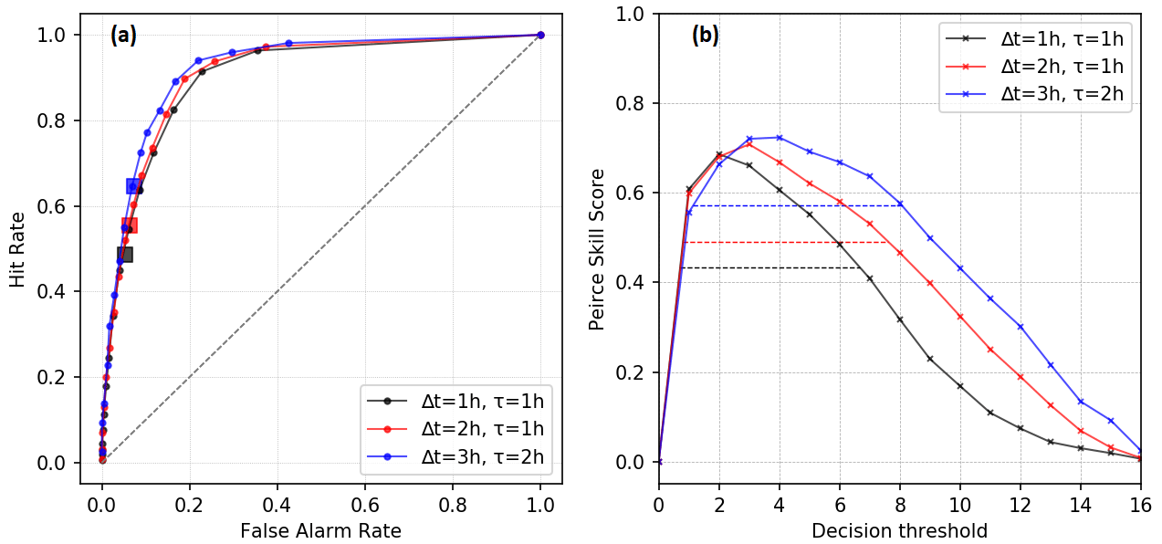
Figure 14 ROC curves(a) and the PSS as a function of decision thresholds (b) of the pX ensemble simulations performed with Pasquill stability classes by aggregating simulations and observations at all stations. There is one curve for each (Δt,τ): $(\mathrm{\Delta }t=\mathrm{1}h,\mathit{\tau }=\mathrm{1}h)$, $(\mathrm{\Delta }t=\mathrm{2}h,\mathit{\tau }=\mathrm{1}h)$, $(\mathrm{\Delta }t=\mathrm{3}h,\mathit{\tau }=\mathrm{2}h)$. The values of the scores for the deterministic pX simulation are indicated by squares in the ROC curves and by horizontal dashed lines in the PSS curves. The diagonal dashed lines are the no-skill lines (H=F).

The pX–Pasquill ensembles have a maximum value of PSS (PSS_max=0.72) corresponding to an optimal decision threshold of three and four members. The ensemble performs better than the deterministic simulation in a range of seven decision thresholds, which represents almost 50 % of the possible values of the decision thresholds. In addition, the ensemble simulations allow the optimization of the decision threshold (Richardson, 2001). These results highlight the robustness of the probabilistic simulations compared to the deterministic simulation in the process of the prediction of threshold exceedances.

To go further into the analysis of the probabilistic performance of the ensembles, the effect of the distance from the source is investigated in Fig. 15. The most representative discretization parameters $(\mathrm{\Delta }t=\mathrm{3}h,\mathit{\tau }=\mathrm{2}h)$ were used to generate dispersion simulations by aggregating data for two groups of stations. The first is a −10 km group which contains stations at distances less than 10 km: PTILH (2 km), Digulleville (2.6 km), Beaumont (4.2 km), and Gréville (5.2 km). The second is a +10 km group which contains stations beyond 10 km: Urville (10.4 km), Ludiver (12.7 km), Octeville (17.7 km), and LRC (18 km).

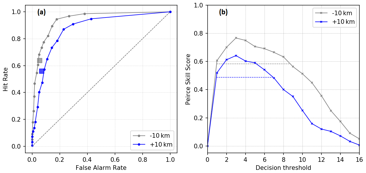
Figure 15 ROC curves (a) and the PSS as a function of decision thresholds (b) of the pX ensemble simulations performed with Pasquill stability classes by aggregating data in the two groups of stations: −10 km (Beaumont, Digulleville, Gréville, and PTILH) and +10 km (LRC, Ludiver, Octeville, and Urville). There is one curve for each group of stations. The scores are calculated using the most optimal discretization configuration $(\mathrm{\Delta }t=\mathrm{3}h,\mathit{\tau }=\mathrm{2}h)$.

The model performs better in the near-field stations. In this case, the ensemble is more efficient than the deterministic simulation in 50 % (8 members) of the decision thresholds, against 37.5 % (6 members) for stations located beyond 10 km. In both cases, the optimal threshold is three members. This better performance in the near-field area may be related to the accumulation of small errors along the plume trajectory that could make the far-range forecast of the peaks more accurate. In addition, peaks at distances farther than 10 km are closest to the background noise, and some errors in the detection of the peaks may be linked to the difficulty in discriminating a peak from the background noise.

With the diffusion laws of Doury (not shown here), the best scores are obtained also for the group of nearest stations to the source in the case of deterministic simulation. However, for the ensembles, there is no significant dependency of the probabilistic scores with respect to the distance from the source.

Taking both meteorological and model uncertainties into account would imply generating an ensemble by also perturbing model parameters (Pasquill/Doury, source elevation, stability). In this perspective, a 32-member super ensemble was generated by combining pX–Pasquill and pX–Doury ensembles. The result (not shown here) is very similar to the pX–Pasquill ensemble, without any notable added value.

5 Conclusions and perspectives

In this study, we explored the potential value of using fine-scale spatial and temporal meteorological ensembles to represent the inherent meteorological uncertainties in ADM outputs. To do so, the high-resolution operational forecasts, AROME-EPS of Météo-France, have been coupled to the Gaussian puff short-range dispersion model, pX of IRSN, to generate a 16-member dispersion ensemble, which accounts for meteorological uncertainties. This paper also proposes an original method to evaluate the ability of a dispersion ensemble to forecast threshold exceedances, using probabilistic scores. For this purpose, we used an original dataset of continuous ⁸⁵Kr air concentration measurements (DISKRYNOC campaign recently conducted by IRSN), along with a well-known source term (every 10 min, provided by the Orano La Hague RP) and meteorological data (NWP from Météo-France and continuous observations from Météo-France/IRSN).

As a first step, the assessment of the quality of the AROME-EPS forecasts, in the North-Cotentin peninsula (northwestern France), was carried out, using meteorological observations over the two-month period of interest (December 2020–January 2021). Wind speed and direction are the most influential variables on the transport of a plume through the atmosphere. For this reason, the meteorological ensembles were evaluated in terms of these 2 meteorological variables in 25 vertical levels within the ABL. The results of this evaluation showed that the AROME-EPS ensembles represent the wind in the ABL with a very acceptable accuracy, despite the slight systematic errors present in the lower layers. Then, an ensemble dispersion modeling chain was implemented using the AROME-EPS forecasts as inputs to the pX model. At this stage, it was necessary to set up a way to combine several 45 h forecasts from different initialization times, and that could be used in the early phase of a nuclear accident. The method proposed in this paper is to use the newest forecast available at the beginning of a day (at 00:00 UTC). This approach can be used to span long periods, in the case of an emergency, by juxtaposing 24 h successive forecasts. Then, two configurations of dispersion simulations were run, with Pasquill and Doury Gaussian standard deviations. A qualitative assessment of the simulations was first presented, to illustrate the ability of some members of the ensemble to forecast peaks while the deterministic simulations failed. The sensitivity of the results to atmospheric stability diagnosis was also highlighted. The probabilistic consistency of the resulting dispersion ensembles was then compared using an innovative method of temporal discretization by sliding intervals, and by calculating two probabilistic scores: ROC curves and PSS. This evaluation process was performed in two parts. First, by comparing the overall performance of the ensemble by aggregating the data from all the measurement stations. Secondly, by comparing the performance of the two configurations in the near fields (stations located less than 10 km from the source) and far fields (stations beyond 10 km from the source). In all cases studied, the best decision threshold was found to be three members, and the ensembles performed better than the deterministic simulations. For operational purposes during emergency situations, this result would imply that when three or more members of the ensemble forecast a threshold exceedance, protective actions should be recommended.

One of the limitations of this study is that it evaluates the performance of the dispersion ensembles by only considering its ability to forecast a value above a given threshold, with a temporal tolerance between the simulated and observed peaks. To complete this evaluation, it would be interesting to develop complementary indicators that evaluate the consistency of dispersion ensembles in term of intensity between the simulated and observed peaks. In addition, since ⁸⁵Kr is a noble gas, this work does not investigate the deposition of radionuclides on the ground, a parameter that would be sensitive to uncertainties in rain forecasts. Thus, it will be interesting to apply the approaches developed in this study to the case of another atmospheric tracer that is not an inert gas, such as radon-222 (Quérel et al., 2022).

Appendix A: Atmospheric stability by classes

A1 Stability classes of Doury (Doury, 1976)

This diagnosis consists in the discretization of the atmospheric stability in two classes: normal diffusion (ND) and low diffusion (LD). While ND corresponds to unstable and neutral situations, LD corresponds to stable situations. In addition, this method is based only on the vertical temperature gradient, which means that it does not take into account the turbulence of mechanical origin:

$$\begin{array}{}\text{(A1)}& {\displaystyle \frac{\partial T}{\partial z}}\left\{\begin{array}{ll}\le -\mathrm{0.5}({}^{\circ }\mathrm{C}/\mathrm{100}\mathrm{m})& :\text{ND},\\ >-\mathrm{0.5}({}^{\circ }\mathrm{C}/\mathrm{100}\mathrm{m})& :\text{LD}.\end{array}\right.\end{array}$$

A2 Stability classes of Pasquill (Pasquill, 1961)

The Pasquill classes allow the discretization of the atmospheric stability in six classes from A (very unstable, coded by 0) to F (very stable, coded by 5). In this article, we have used two diagnostics of calculating of the Pasquill classes:

• Method of Turner (Turner, 1969). Based on the 10 m wind speed and the surface solar radiation downwards (during daytime) or total cloud cover (at night) (Table A1), this diagnostic has the advantage of taking into account the two origins of turbulence: mechanical (wind) and thermal (solar radiation).

• Method of temperature gradient (Seinfeld and Pandis, 1998). Based on the temperature difference over 100 m (Table A2), this diagnosis does not take into account the turbulence of mechanical origin, but it captures variations in stability conditions better than the Doury diagnosis.

Table A1 Pasquill classes according to the method of Turner.

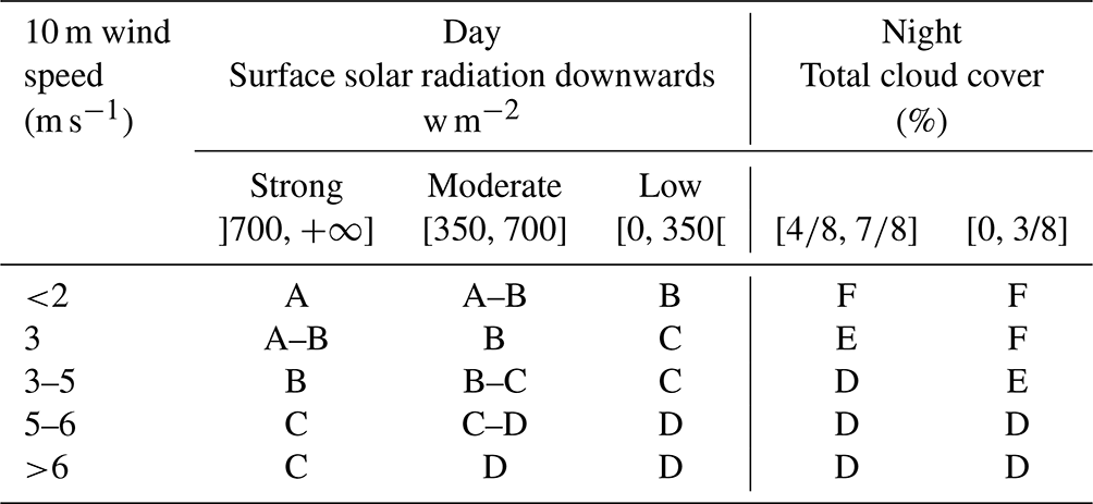
Table A2 Pasquill classes according to method of temperature gradient, and correspondence with the classes of Doury.

Appendix B: Formulas for Gaussian standard deviations

The aim is to calculate the evolution of standard deviations of the concentration distribution which is given by

$$\begin{array}{}\text{(B1)}& \mathit{\sigma }(t+\mathrm{d}t)=\mathit{\sigma }\left(t\right)+{\displaystyle \frac{\mathrm{d}\mathit{\sigma }}{\mathrm{d}t}}\mathrm{d}t=\mathit{\sigma }\left(t\right)+{\displaystyle \frac{\mathrm{d}\mathit{\sigma }}{\mathrm{d}x}}U\mathrm{d}t,\end{array}$$

where t and x are time and distance since the emission of the puff, respectively; U is the speed of advection of the puff.

Thus, the problem is deferred to the determination of $\frac{\mathrm{d}\mathit{\sigma }}{\mathrm{d}x}$ (or $\frac{\mathrm{d}\mathit{\sigma }}{\mathrm{d}t}$) in each time step t. For a given standard deviation law, we have $\mathit{\sigma }\left(x\right)=f(x,{\mathit{\alpha }}_{\mathrm{1}},{\mathit{\alpha }}_{\mathrm{2}},\mathrm{\dots },{\mathit{\alpha }}_n)$, where α_i are parameters that depend on the atmospheric stability, and are determined empirically. Then, $\frac{\mathrm{d}\mathit{\sigma }}{\mathrm{d}x}$ can be expressed as follows:

$$\begin{array}{}\text{(B2)}& \begin{array}{rl}& \left\{\begin{array}{l}\frac{\mathrm{d}\mathit{\sigma }}{\mathrm{d}x}=\frac{\partial f}{\partial x}(x,{\mathit{\alpha }}_{\mathrm{1}},{\mathit{\alpha }}_{\mathrm{2}},\mathrm{\dots },{\mathit{\alpha }}_n)\\ x=f^{-\mathrm{1}}\left(\mathit{\sigma }\right)\end{array}\right.\\ & \iff {\displaystyle \frac{\mathrm{d}\mathit{\sigma }}{\mathrm{d}x}}={\displaystyle \frac{\partial f}{\partial x}}\left(f^{-\mathrm{1}}\right(\mathit{\sigma }),{\mathit{\alpha }}_{\mathrm{1}},{\mathit{\alpha }}_{\mathrm{2}},\mathrm{\dots },{\mathit{\alpha }}_n).\end{array}\end{array}$$

A similar reasoning is possible for $\frac{\mathrm{d}\mathit{\sigma }}{\mathrm{d}t}$. Depending on the complexity of the function f, it will be more or less easy to express the function $\frac{\mathrm{d}\mathit{\sigma }}{\mathrm{d}x}$.

• Pasquill laws.

  $$\begin{array}{}\text{(B3)}& \mathit{\sigma }=a{x}^b+c\Rightarrow {\displaystyle \frac{\mathrm{d}\mathit{\sigma }}{\mathrm{d}x}}=ab{\left({\displaystyle \frac{\mathit{\sigma }}{a}}\right)}^{\frac{b-\mathrm{1}}{b}},\end{array}$$

  where the parameters a, b, and c are determined according to the Pasquill stability classes.

• Doury laws.

  $$\begin{array}{}\text{(B4)}& \mathit{\sigma }=A{t}^k{t}^{k-\mathrm{1}}\Rightarrow {\displaystyle \frac{\mathrm{d}\mathit{\sigma }}{\mathrm{d}x}}=kA{\mathit{\sigma }}^{\frac{k-\mathrm{1}}{k}},\end{array}$$

  where the parameters A and k are determined according to the Doury stability classes and depend on transfer time since release time.