the Creative Commons Attribution 4.0 License.
the Creative Commons Attribution 4.0 License.
 | 08 Dec 2022
How do Cl concentrations matter for the simulation of CH4 and δ13C(CH4) and estimation of the CH4 budget through atmospheric inversions?
Joël Thanwerdas
Marielle Saunois
Isabelle Pison
Didier Hauglustaine
Antoine Berchet
Bianca Baier
Colm Sweeney
Philippe Bousquet
Atmospheric methane (CH4) concentrations have been rising since 2007 due to an imbalance between CH4 sources and sinks. The CH4 budget is generally estimated through top-down approaches using chemistry transport models (CTMs) and CH4 observations as constraints. The atmospheric isotopic CH4 composition, δ13C(CH4), can also provide additional constraints and helps to discriminate between emission categories. Nevertheless, to be able to use the information contained in these observations, the models must correctly account for processes influencing δ13C(CH4). The oxidation by chlorine (Cl) likely contributes less than 5 % to the total oxidation of atmospheric CH4. However, the large kinetic isotope effect of the Cl sink produces a large fractionation of 13C, compared with 12C in atmospheric CH4, and thus may strongly influence δ13C(CH4). When integrating the Cl sink in their setup to constrain the CH4 budget, which is not yet standard, atmospheric inversions prescribe different Cl fields, therefore leading to discrepancies between flux estimates. To quantify the influence of the Cl concentrations on CH4, δ13C(CH4), and CH4 budget estimates, we perform sensitivity simulations using four different Cl fields. We also test removing the tropospheric and the entire Cl sink. We find that the Cl fields tested here are responsible for between 0.3 % and 8.5 % of the total chemical CH4 sink in the troposphere and between 1.0 % and 1.6 % in the stratosphere. Prescribing these different Cl amounts in atmospheric inversions can lead to differences of up to 53.8 Tg CH4 yr−1 in global CH4 emissions and of up to 4.7 ‰ in the globally averaged isotopic signature of the CH4 source δ13C(CH4)source), although these differences are much smaller if only recent Cl fields are used. More specifically, each increase by 1000 in the mean tropospheric Cl concentration would result in an adjustment by +11.7 Tg CH4 yr−1, for global CH4 emissions, and −1.0 ‰, for the globally averaged δ13C(CH4)source. Our study also shows that the CH4 seasonal cycle amplitude is modified by less than 1 %–2 %, but the δ13C(CH4) seasonal cycle amplitude can be significantly modified by up to 10 %–20 %, depending on the latitude. In an atmospheric inversion performed with isotopic constraints, this influence can result in significant differences in the posterior source mixture. For example, the contribution from wetland emissions to the total emissions can be modified by about 0.8 % to adjust the globally averaged δ13C(CH4)source, corresponding to a 15 Tg CH4 yr−1 change. This adjustment is small compared to the current wetland source uncertainty, albeit far from negligible. Finally, tested Cl concentrations have a large influence on the simulated δ13C(CH4) vertical profiles above 30 km and a very small impact on the simulated CH4 vertical profiles. Overall, our model captures the observed CH4 and δ13C(CH4) vertical profiles well, especially in the troposphere, and it is difficult to prefer one Cl field over another based uniquely on the available observations of the vertical profiles.
- Article
(5362 KB) - Full-text XML
-
Supplement
(2922 KB) - BibTeX
- EndNote


Methane (CH4) is a very important species for both atmospheric chemistry and climate. Its atmospheric mole fractions have reached an average of 1896 ppb (parts per billion) at the surface in 2021 (Dlugokencky, 2022), which is almost 3 times higher than the preindustrial mole fractions (Etheridge et al., 1998). After a plateau between 1999 and 2006, CH4 mole fractions resumed their increase in 2007, without showing any sign of stabilization since then. The increase has even reached an unprecedented value of +16.9 ppb for the year 2021 (Dlugokencky, 2022). The accumulation of CH4 (∼8 ppb yr−1, on average, since 2007) in the atmosphere is the result of an imbalance of about 20 Tg CH4 yr−1 (Saunois et al., 2020) between sources that release CH4 into the atmosphere and sinks that remove it. Sinks are mostly due to oxidation reactions in the atmosphere between CH4 and three radicals, i.e., hydroxyl (OH), atomic oxygen (O1D), and chlorine (Cl). These chemical reactions account for about 93 % of the CH4 sink, with the remainder being removed by methanotrophic bacteria in the soil (Saunois et al., 2020). On the other hand, CH4 sources are varied and result from radically different processes (biogenic, thermogenic, and pyrogenic).
Estimating global CH4 sources with accuracy is a mandatory, yet challenging, step towards implementing efficient emission mitigation policies. Top-down atmospheric inversions are known to be efficient approaches for estimating CH4 sources at different scales and have become increasingly relevant over the years as observational networks have developed (Houweling et al., 2017, and references therein). However, inversions that assimilate only CH4 observations can only rely on variations in seasonal cycles to differentiate co-located emissions. To better separate these sources, assimilating observations of the isotope ratio in atmospheric CH4, or δ13C(CH4), can be relevant. This value is based on the ratio between the isotopologue 12CH4, which represents about 99 % of the CH4 in the atmosphere (Stolper et al., 2014) and its counterpart 13CH4. δ13C(CH4) is commonly defined using a deviation of the sample atomic isotopic ratio relative to a specific standard ratio as follows:
R represents the abundance of 13C relative to 12C in all CH4 molecules. Rstd=0.0112372 is here the standard ratio of Vienna Pee Dee Belemnite (VPDB; Craig, 1957).
CH4 sources exhibit specific isotopic signatures that are mainly controlled by the process involved in the production of CH4. Broadly summarized, most biogenic sources have an isotopic signature between −65 ‰ and −55 ‰, thermogenic sources between −50 ‰ and −30 ‰, and pyrogenic sources between −25 ‰ and −15 ‰ (Sherwood et al., 2017), although the full distributions of these signatures are very large, with overlapping values. The post-2007 CH4 increase is notably associated with a decrease in the atmospheric isotopic composition δ13C(CH4) (Nisbet et al., 2019) that could help to better explain the renewed CH4 growth and, more specifically, the contribution from the different CH4 sources to it.
The sinks also have an influence on δ13C(CH4), as they remove 12CH4 faster than 13CH4. This effect, called the kinetic isotope effect (KIE), hereinafter also referred to as isotopic fractionation, is quantified using the ratio of the reaction rate constants X+12CH4 and X+13CH4 with X the species of interest (X = OH, O(1D) or Cl). KIE, with and being the oxidation reaction rate constants. As a result, δ13C(CH4) depends on both sources and sinks, like CH4, but also on the isotopic fractionation and the isotopic signatures of the sources.
Among all CH4 sinks, the Cl sink accounts for a small part of the total CH4 oxidation. Following the discovery of the dramatic impact of Cl on ozone in the stratosphere, many studies have focused on the impact of stratospheric Cl on CH4 and δ13C(CH4) using box or 2-D models (e.g., Röckmann et al., 2004; McCarthy et al., 2003; Wang et al., 2002; McCarthy et al., 2001; Saueressig et al., 2001; Gupta et al., 1996; Müller et al., 1996). McCarthy et al. (2003) estimated that Cl was responsible for 20 %–35 % of CH4 removal in the stratosphere. Saunois et al. (2020) suggested a range of values for the total stratospheric sink between 12 and 37 Tg CH4 yr−1, leading to a plausible stratospheric Cl sink of 2–13 Tg CH4 yr−1 or about only 0.4 %–2.4 % of the total CH4 oxidation in the atmosphere. Although this contribution is very small, the Cl sink is particularly important because of its large fractionation effect (KIE = 1.066 for the Cl sink against 1.0039 for the OH sink; see Sect. 2.1). The aforementioned studies showed that stratospheric Cl has a strong impact on δ13C(CH4), not only in the stratosphere but also closer to the surface. In particular, Wang et al. (2002) estimated that stratospheric Cl was responsible for a δ13C(CH4) enhancement of 0.23 ‰ at the surface between 1970 and 1992 due to stratosphere–troposphere exchanges (STEs).
In the troposphere, the Cl sink likely accounts for less than 5 % of CH4 oxidation (Wang et al., 2019, 2021; Hossaini et al., 2016; Sherwen et al., 2016b; Gromov et al., 2018; Allan et al., 2007). Several studies have estimated Cl concentrations in the troposphere and in the marine boundary layer (MBL) and discussed the Cl sink. Allan et al. (2007) estimated the Cl sink in the troposphere to be 25 Tg CH4 yr−1, representing about 5 % of the total CH4 chemical sink. More recently, Hossaini et al. (2016), Sherwen et al. (2016b), Wang et al. (2019), and Wang et al. (2021) have made important developments in tropospheric chemistry modeling (see Sect 2.2) and obtained oxidation contributions of 2.6 %, 2 %, 1 %, and 0.8 %, respectively, with mean tropospheric Cl concentrations between 620 and 1300 . However, Gromov et al. (2018) concluded that variations in Cl concentrations above 900 in the extratropical part of the Southern Hemisphere are very unlikely, thus suggesting that the high estimates from Allan et al. (2007) and Hossaini et al. (2016) are likely overestimated. This estimated range of oxidation contributions may appear small, but Strode et al. (2020) recently showed a high sensitivity of the tropospheric δ13C(CH4) distribution to the variation in Cl fields by testing, among others, those of Allan et al. (2007), Sherwen et al. (2016b), and Hossaini et al. (2016), indicating that each percent increase in how much CH4 is oxidized by Cl leads to a 0.5 ‰ increase in δ13C(CH4), which is, therefore, larger than the global downward shift that has been observed since 2007 (Nisbet et al., 2019).
Forward and inverse 3-D modeling studies focusing on CH4 and δ13C(CH4) consider the Cl sink at a different level of detail. Most studies consider only the Cl sink in the stratosphere (e.g., Fujita et al., 2020; Rigby et al., 2012; Monteil et al., 2011; Fletcher et al., 2004) and very few account for tropospheric Cl only (e.g., Thompson et al., 2018). In single-box models, sinks are combined, and an overall fractionation coefficient is used (e.g., Schaefer et al., 2016; Schwietzke et al., 2016). In recent studies, Cl is often prescribed in both the troposphere and stratosphere (e.g., McNorton et al., 2018; Rice et al., 2016; Warwick et al., 2016; Neef et al., 2010), although most studies use the Cl distribution suggested by Allan et al. (2007), which is likely to be overestimated, as mentioned above.
In the atmospheric inversions performed with the model LMDz (Laboratoire de Méteorologie Dynamique-Zoom) coupled to the Simplified Atmospheric Chemistry System (SACS), the Cl sink was omitted, even in the stratosphere, the Cl sink was omitted, even in the stratosphere (Saunois et al., 2020; Locatelli et al., 2015; Pison et al., 2009; Bousquet et al., 2006). For these studies assimilating only CH4 mixing ratio observations, the impact of the Cl sink on the estimated CH4 emissions was considered negligible. However, the number and quality of isotopic observations have considerably increased since the 2000s, and developments in the Community Inversion Framework (CIF; Berchert et al., 2021) have been made in order to use the isotopic constraint with the CIF-LMDz-SACS inversion system (Thanwerdas et al., 2022). Joint assimilation (CH4 and δ13C(CH4)) is proving to be relevant and necessary in order to reconcile the estimated CH4 budgets with the observed atmospheric isotope composition. Considering the large impact of the Cl sink on δ13C(CH4), it is necessary to include and evaluate the Cl sink and its impact on the simulation of CH4 and δ13C(CH4) with our model.
Here, we detail the influence of tropospheric and stratospheric Cl on the modeling of CH4 and δ13C(CH4) in LMDz-SACS by using several Cl fields. The ultimate aim is to assimilate the isotopic composition observations to perform multi-constraint inversions with the LMDz-SACS model. Therefore, the developments performed and the results obtained are analyzed through the prism of atmospheric inversion. In Sect. 2, we present the characteristics of the available Cl fields, model inputs, and observations used for evaluation. In Sect. 3, we analyze the influence of the different Cl fields on CH4 and δ13C(CH4) at the surface, on the global CH4 flux and δ13C(CH4) source signature adjustment obtained with inversion methods, and on the CH4 and δ13C(CH4) vertical profiles.
2.1 The chemistry transport model (CTM)
The general circulation model (GCM) LMDz is the atmospheric component of the coupled model of the Institut Pierre-Simon Laplace (IPSL-CM) developed at the Laboratoire de Météorologie Dynamique (LMD; Hourdin et al., 2006). The version of LMDz used here is an offline version dedicated to the inversion framework created by Chevallier et al. (2005); the precalculated meteorological fields provided by the online version of LMDz are given as input to the model, which considerably reduces the computation time. The model is built at a horizontal resolution of 3.8∘ × 1.9∘ (96 grid cells in longitude and latitude), with 39 hybrid sigma pressure levels reaching an altitude of about 75 km. About 20 levels are located in the stratosphere and above. The time step of the model is 30 min, and the output values have a resolution of 3 h. Horizontal winds have been nudged towards the ECMWF meteorological analyses (ERA-Interim) in the online version of the model. Vertical diffusion is parameterized by a local approach of Louis (1979), and deep convection processes are parameterized by the scheme of Tiedtke (1989). The offline model LMDz, coupled with the Simplified Atmospheric Chemistry System (SACS) module (Pison et al., 2009), was previously used to simulate atmospheric mole fractions of trace gases such as CH4, carbon monoxide (CO), methyl chloroform (MCF), formaldehyde (CH2O), or hydrogen (H2). This system has been recently converted into a chemistry parsing system (Thanwerdas et al., 2022). It follows the principle of the chemical parsing system of the regional model CHIMERE (Mailler et al., 2017; Menut et al., 2013) and allows the user to prescribe the set of chemical reactions to consider. Consequently, it generalizes the SACS module to any set of possible reactions. The concentration fields of the different species are either prescribed or simulated. Prescribed species (here OH, O(1D), and Cl) are not transported in LMDz, and their mole fractions are not updated by chemical production or destruction. These species are only used to calculate reaction rates and update the mole fractions of transported species at each iteration of the model. In this study, the 12CH4 and 13CH4 isotopologues are simulated as separate tracers and CH4 mole fractions are defined as the sum of the mole fractions of the two isotopologues. Oxidation by Cl was added to complete the chemical removal of CH4, which only considered OH + CH4 and O(1D) + CH4 reactions in the original SACS chemical scheme. The photolysis of CH4 is not included in SACS, as it is considered negligible. None of the inversion studies mentioned above, in particular those of Saunois et al. (2020), accounted for this sink.
Reactions between 12CH4 and OH, O(1D), and Cl are represented by the chemical equations below, and similar equations apply to 13CH4, as follows:
Three-dimensional and time-dependent oxidant concentration fields (OH, O(1D), and Cl) were simulated by the GCM LMDz coupled to the INteraction with Chemistry and Aerosols (INCA) model (Hauglustaine et al., 2021; Folberth et al., 2006; Hauglustaine et al., 2004). A total of 17 ozone-depleting substances consisting of chlorofluorocarbons (CFCs; CFC-12, CFC-11, and CFC-113), three hydrochlorofluorocarbons (HCFCs; HCFC-22, HCFC-141b, and HCFC-142b), two halons (halon-1211 and halon-1301), methyl chloroform (CH3CCl3 or MCF), carbon tetrachloride (CCl4), methyl chloride (CH3Cl), methylene chloride (CH2Cl2), chloroform (CHCl3), methyl bromide (CH3Br), and HFC-134a, and their associated photochemical reactions, were included in the INCA chemical scheme to produce Cl radicals (Terrenoire et al., 2022). In the coupled LMDz-INCA simulations, surface concentrations of these long-lived Cl precursors were prescribed based on historical data sets prepared by Meinshausen et al. (2017). The model was run for the 1850–2018 period (Hauglustaine et al., 2021).
Saueressig et al. (2001)Saueressig et al. (1995)Saueressig et al. (2001)Saueressig et al. (2001)Table 1Reaction rate constants and KIEs of CH4 chemical sinks. The reaction rate constants are taken from Burkholder et al. (2015).
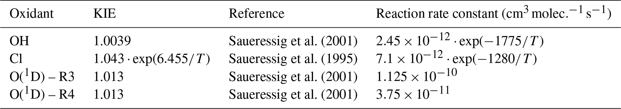
All reaction rate constants and associated values used in LMDz-SACS are given in Table 1. The reaction rate constants with 13CH4 are modified based on the definition of the KIE. Few studies have evaluated the KIEs associated with CH4 chemical sinks (particularly for O(1D) and Cl) over a wide range of temperatures, and thus large uncertainties remain. For CH4 + OH, we adopted the value of Saueressig et al. (2001), as it indicates that these data are of considerably higher experimental precision and reproducibility than previous studies, in particular Cantrell et al. (1990), who suggested a value of 1.0054.
2.2 Description of Cl fields
Four fields of Cl are compared in this study. Two fields were generously provided by the respective authors of Sherwen et al. (2016b) and Wang et al. (2021). They will be referred to as the Cl-Sherwen and Cl-Wang fields. Sherwen et al. (2016b) obtained the associated Cl field using version 10 of the GEOS-Chem CTM (https://geos-chem.seas.harvard.edu/, last access: 11 November 2022) running at a 4∘ × 5∘ spatial resolution. Previously, Sherwen et al. (2016a) extended the stratospheric chlorine scheme to the troposphere. Sherwen et al. (2016b) improved the coupling of halogens (Br, Cl, and I) chemistry and further updated the chlorine chemistry scheme. Subsequently, Wang et al. (2019) focused principally on the modeling of tropospheric reactive chlorine by developing the treatment of sea salt aerosol (SSA) chloride and chlorine gases, in addition to SSA acid displacement thermodynamics, starting from version 11-02d of GEOS-Chem. Chloride mobilization from SSA by the acid displacement of HCl represents a significant source of reactive chlorine in the troposphere. The authors also mentioned a better accounting of other chlorine sources (combustion, organochlorines, transport from the stratosphere, and anthropogenic HCl) compared to previous versions. Wang et al. (2020, 2021) made some additional developments that appear to have a relatively small impact on the atomic Cl spatial distribution and mean concentration in the troposphere. They did not include continental anthropogenic emissions of inorganic Cl (coal combustion, waste incineration, and industrial activities) because existing estimates are likely outdated and carry too high uncertainties. Consequently, the Cl concentrations from Wang et al. (2021) may be underestimated over regions where relatively high anthropogenic chlorine sources have been reported (e.g., China).
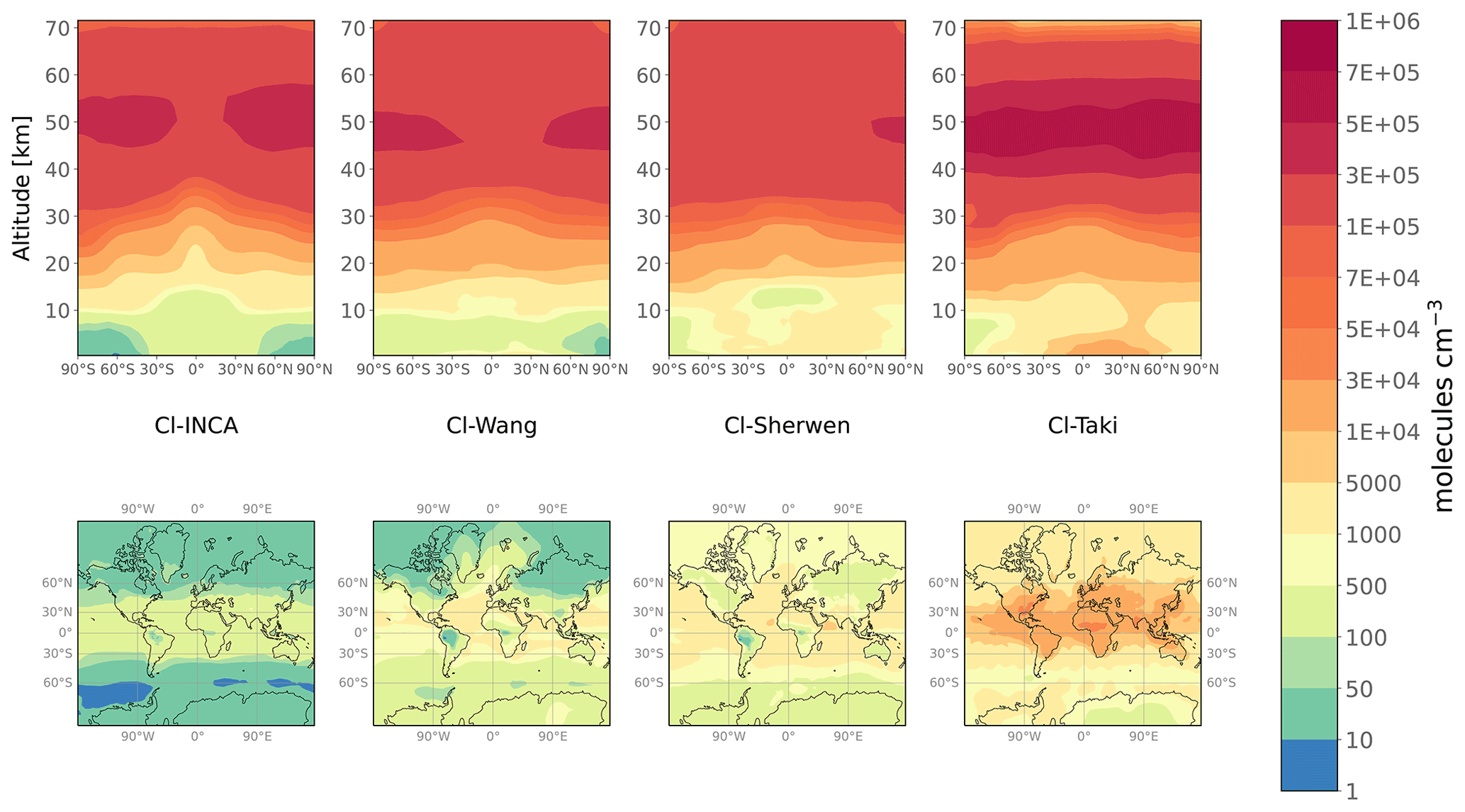
Figure 1Annual mean meridional cross section (upper panels) and tropospheric Cl concentrations (lower panels) for the four 3-D fields Cl-INCA, Cl-Wang, Cl-Sherwen, and Cl-Taki.
Another field was simulated by the LMDz-INCA model, as mentioned in Sect. 2.1. This field will be referred to as the Cl-INCA field. At present, simulations performed with the LMDz-INCA model do not fully represent the chemical interactions between Cl and other species in the troposphere. In particular, developments are currently being made to improve the treatment of SSA and chloride mobilization from SSA. Cl-INCA did not benefit from such enhancements, resulting in significant discrepancies compared to Cl-Wang and Cl-Sherwen. The mean tropospheric Cl concentration (330 ) in the Cl-INCA field is about half of the tropospheric mean (630 ) of Wang et al. (2021) but is in agreement with the upper limits inferred by Gromov et al. (2018).
The last field was simulated by version 5.7b of the CCSR/NIES/FRCGC (Center for Climate System Research/National Institute for Environmental Studies/Frontier Research Center for Global Change) atmospheric GCM (Takigawa et al., 1999). This was provided by the GCP-GMB (Global Carbon Project–Global Methane Budget) team to run the inversions used in Saunois et al. (2020), although some inversions did not prescribe it. The model did not include any treatment of SSA and chloride mobilization from SSA. More generally, it did not include any representation of tropospheric reactive chlorine chemistry. We could not have access to additional information regarding this field. It is referred to as the Cl-Taki field.
The four fields are shown in Fig. 1. We use the lapse rate (2 K km−1) definition from the World Meteorological Organization (WMO) and the meteorological fields from the online LMDz model to define the tropopause. Global mean tropospheric Cl concentrations range from 330 (Cl-INCA) to 4730 (Cl-Taki). The zonal relative changes in tropospheric concentrations are similar, although Cl-Wang, Cl-Sherwen, and Cl-Taki have a greater spatial variability around their mean value than Cl-INCA, especially in the mid-latitudes (75 %, 66 %, and 63 % against 36 %, respectively). Cl-Wang, Cl-Sherwen and Cl-INCA exhibit similar concentrations in the stratosphere ( ). The increase in concentrations with altitude between the surface and 30 km is similar between all fields, with a 0–30 km vertical gradient of . Stratospheric concentrations are, however, larger in Cl-Taki, reaching a mean value of 2.1×10⁵ .
In this study, we do not test the Cl fields from Hossaini et al. (2016) and Allan et al. (2007) because the fields presented above cover a range of tropospheric and stratospheric Cl concentrations wide enough to carry out a robust analysis.
2.3 Description of simulations
The time period adopted for all simulations here is 1998–2018. Mole fractions of 12CH4 and 13CH4 are simulated over this period of time in multiple simulations, either forward or inverse.
First, a set of optimized fluxes and source signatures are obtained by running atmospheric variational inversions over 1998–2018 based on a joint assimilation of CH4 and δ13C(CH4) in the CIF-LMDz-SACS system designed by Thanwerdas et al. (2022). A variational inversion consists of performing alternate runs of the CTM's forward and adjoint codes to calculate the cost function and its gradient. A global minimum of this cost function is then sought using an adequate minimization algorithm. With our method, multiple iterations of this process are performed until a satisfactory convergence criterion is reached. At the end of the minimization process, we obtain posterior fluxes and source signatures that reduce the discrepancies between observed and simulated CH4 and δ13C(CH4), compared with prior estimates. This system runs a last forward simulation with optimized inputs at the end of the inversion process.
One variational inversion is run for each Cl field presented in Sect. 2.2. The Cl-Wang, Cl-Sherwen, Cl-Taki, and Cl-INCA fields are used in the INV-Wang, INV-Sherwen, INV-Taki, and INV-INCA inversions, respectively. In Saunois et al. (2020), the majority of the inversions were performed without a tropospheric Cl sink; thus, we perform one inversion using the Cl-Wang field but without a tropospheric Cl (INV-NoTropo). Finally, as LMDz-SACS completely omitted the Cl sink in previous studies, we estimate the errors generated by this omission by running a last inversion without a Cl sink (INV-NoCl). More information about the variational inversion method, the inversion system used here, and the setup of these inversions is provided in the Supplement (Sect. S1). Apart from the prescribed Cl field, all these inversions share the same configuration. Consequently, for each inversion, we obtain a different set of fluxes and source signatures, and the differences between them result only from the influence of Cl concentrations. These differences are analyzed in Sect. 3.3 and 3.4.
As mentioned above, the last forward simulation of a variational inversion is performed with optimized inputs. Hereinafter, INV-* outputs (simulated values) refer to the results of the last forward simulation performed with the optimized fluxes and source signatures derived from the corresponding inversion, which are prescribed as monthly fields at the horizontal resolution of the model. As expected, CH4 and δ13C(CH4) simulated with the posterior fluxes and source signatures are all consistent with the assimilated observations (see Fig. S1). Emissions and source isotopic signatures obtained with INV-Wang are given in Table 2. They both vary over time and space.
A set of simple forward simulations (FWD-*) with identical prescribed fluxes and source signatures are also run to quantify the biases in CH4 and δ13C(CH4) that arise from differences in prescribed Cl field, hence leading to differences in atmospheric sink. The posterior fluxes and source signatures from INV-Wang are used for all FWD-* simulations because the Cl-Wang field is taken from the most comprehensive and recent study to date. A different Cl field is prescribed for each simulation, resulting in six forward simulations, i.e., FWD-Wang, FWD-Sherwen, FWD-Taki, FWD-INCA, FWD-NoTropo, and FWD-NoCl. Apart from the prescribed Cl field, all these simulations adopt the same configuration. Consequently, note that the FWD-Wang and INV-Wang inputs and outputs are identical.
To summarize, our simulations are as follows:
-
INV-* outputs are consistent with observed CH4 and δ13C(CH4) because they use optimized fluxes and source signatures derived from a variational inversion.
-
Apart from FWD-Wang, FWD-* outputs are not consistent with observed values because they all adopt the same fluxes and source signatures.
Table 2Global CH4 emissions and associated flux-weighted isotopic signatures by source category obtained with INV-Wang. The given values are averages over 1998–2018. Values in parentheses are the minimum and maximum over this period of time (min/max).
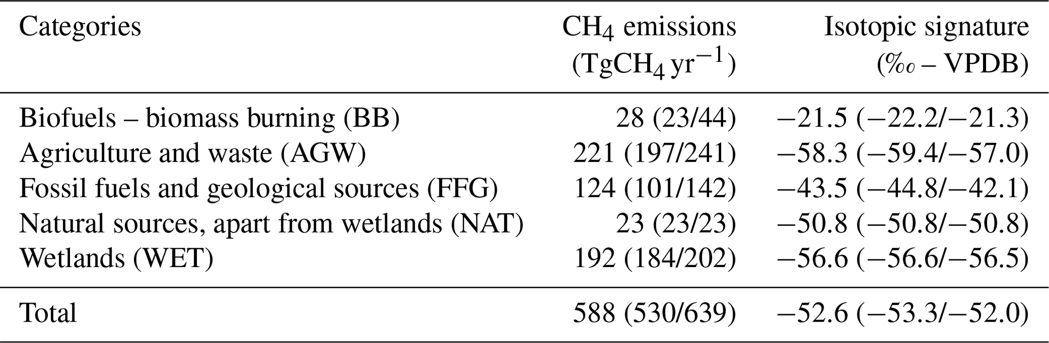
Table 3Nomenclature and description of the sensitivity tests performed in this study. The INV-* simulations refer to both the variational inversion performed with the system of Thanwerdas et al. (2022) and to the final forward simulation of this inversion process with the associated optimized fluxes and source signatures. For each test, the model used to simulate Cl concentrations is given. Forward sensitivity tests (FWD-*) have also been run with identical optimized fluxes and source signatures based on the INV-Wang outputs. Note that INV-Wang and FWD-Wang are identical.

2.4 Observations
Different data sets of observations are either assimilated in our inversions or used to evaluate our simulations and to estimate the impact of the Cl field. These observations are of several types, namely surface measurements of CH4 and δ13C(CH4), in situ vertical profiles of CH4, and in situ vertical profiles of δ13C(CH4).
CH4 observations taken at 79 surface stations of the Global Greenhouse Gas Reference Network (GGGRN), part of the NOAA-ESRL's Global Monitoring Laboratory (NOAA GML), are assimilated in the inversions introduced in Sect. 2.3. Reported uncertainties are generally below 5 ppb. δ13C(CH4) measurements provided by the Institute of Arctic and Alpine Research (INSTAAR) by analyzing air samples collected at 22 stations on an approximately weekly basis are also assimilated (White et al., 2021). Reported uncertainties are generally below 0.15 ‰. The station locations and additional information can be found in Fig. S3 and Tables S6 and S7.
The analysis of the impact of Cl on CH4 vertical profiles is conducted using a set of 115 AirCore profiles recovered from 11 different sites over the 2012–2018 period. A total of 80 profiles are provided by the NOAA GML aircraft program (Baier et al., 2021; Karion et al., 2010) and 35 other profiles by the French AirCore program (Membrive et al., 2017). The balloon-borne AirCore technique (Karion et al., 2010) allows air samples to be taken from the stratosphere (up to approximately 30 km) to the ground, upon a parachute-based descent. Figure S4 and Table S4 in the Supplement provide information about the provider, location, and number of profiles collected. Reported uncertainties generally increase with altitude due to end-member mixing within the AirCore samples. They are below 2 ppb in the troposphere and can reach 10 ppb in the lower stratosphere.
We also use air samples from stratospheric balloon flights analyzed in Röckmann et al. (2011) to compare simulated vertical profiles of δ13C(CH4) to observations. Figure S5 and Table S5 in the Supplement provide information about the time, location, and number of profiles collected. The samples were retrieved at four different locations, from subtropical to high latitudes, above an altitude of 10 km and up to 35 km. Uncertainties are generally below 0.2 ‰.
2.5 Estimating global CH4 flux and δ13C(CH4) source signature adjustments
Three methods are employed to quantify the influence of the Cl sink on inversions adjusting both CH4 fluxes and isotopic signatures of sources, here denoted by δ13C(CH4)source. Simple descriptions of the three methods are provided here, whereas comprehensive descriptions are given in the Supplement (Sects. S1, S2, and S3).
The first approach (M1) is based on the INV-* inversions presented in Sect. 2.3 and the 3-D variational inversion system from Thanwerdas et al. (2022). Although this approach is the most robust among the three methods used here, the associated computational burden is also the largest. At present, approximately 4 months (wall clock time on LSCE computational clusters consisting of Intel® Xeon® Gold 5317 central processing units (CPUs) with a frequency of 3.00 GHz) are necessary to reach a satisfactory convergence criterion with this system for a 20-year assimilation window, which is highly excessive if one must use this method every time the influence of two Cl fields are to be compared. Only a maximum of 8–10 CPUs can be used in parallel to run the CIF-LMDz-SACS code. Additional CPUs do not reduce the wall clock computational time due to input/output (I/O) limits. Here, we employ this method to (1) take advantage of the high spatial resolution of the CIF-LMDz-SACS system and thus perform the analysis at smaller spatial scales and (2) demonstrate that the simpler methods presented below provide good results at the global scale. Optimized CH4 fluxes and source signatures are directly taken from the INV-* results. More information is provided in Sect. S1.
The second approach (M2) employs a box model analytical inversion system assimilating both CH4 and δ13C(CH4) observations. This system has been specifically designed for the purpose of this study. The 12CH4 and 13CH4 mole fractions in the troposphere are simulated with this box model, converted to CH4 mole fractions and δ13C(CH4) values, and compared to globally averaged observations provided by the NOAA GML. An analytical nonlinear method is then applied to find the optimal solution of the inversion problem. This method is extremely simple to use and very fast (∼1 min of wall clock time with a regular laptop) but requires the input parameters of the box model (global lifetime, KIE, and conversion factor between CH4 mass and mole fractions) to be computed prior to the inversion. Here, these input parameters are derived from the forward simulations described in Sect. 2.3. More information is provided in Sect. S2.
The third approach (M3) is not an inversion in its strictest definition. It is only based on an analysis of the time series of the bias in CH4, 12CH4, and 13CH4 total atmospheric masses between two forward simulations (FWD-*) described in Sect. 2.3. This bias increases over time but stabilizes after several decades. We derive a simple theoretical framework to predict the adjustment value that an inversion system would have to apply to the prior global CH4 flux and the globally averaged δ13C(CH4)source in order to offset this bias. More information is provided in Sect. S3. This method is less robust than the other ones but does not require performing an inversion. In Sect. 3.3 and 3.4, we show that M3 provides results that are very consistent with M1 and M2.
3.1 Quantification of the Cl sink
The simulated chemical sink of CH4 due to Cl oxidation varies depending on the prescribed Cl field. Table 4 summarizes the multiple estimates averaged over the 1998–2018 period in both the troposphere and stratosphere. Also included in the comparison are the tropospheric Cl sink estimates from Hossaini et al. (2016) and Allan et al. (2007), and the stratospheric Cl sink estimate from Patra et al. (2011). All of them are used in many CH4 inversions. The Cl sink used in Patra et al. (2011), which is exclusively stratospheric, is the sum of O(1D) and Cl sinks. Contributions of O(1D) and Cl sinks to the stratospheric sink were previously estimated to be 20 %–40 % and 20 %–35 %, respectively (McCarthy et al., 2003; Rice et al., 2003). Using these estimates, the Cl sink from Patra et al. (2011) should contribute between 1.3 % and 2.6 % of the total sink. Using our estimates of O(1D) concentrations obtained with LMDz-INCA (see Sect. 2.1), we obtain a Cl contribution of 2.6 %.
Based on our simulations, contributions from the tropospheric Cl sink with Cl-Wang (0.6 %) and Cl-Sherwen (1.8 %) are slightly lower than those given in the associated papers (i.e., 0.8 % and 2 %, respectively). This discrepancy is likely due to a slight difference in the definition of the tropopause height or/and in the prescribed OH sink that is used to calculate the total chemical sink.
The tropospheric sink provided by Allan et al. (2007) is well above the other recent values. The tropospheric sink estimated by Hossaini et al. (2016), used in recent studies (Saunois et al., 2020; McNorton et al., 2018), is also slightly above that inferred with Cl-Sherwen (Table 4; 1.4 times higher) but well above those inferred with Cl-Wang and Cl-INCA (4 and 8.5 times higher). In the troposphere, the sink inferred with Cl-Taki is much larger than the other sinks (up to 28 times larger) and therefore even larger than the value suggested by Allan et al. (2007), which is already very likely to be overestimated (Gromov et al., 2018). In the stratosphere, this Cl-Taki sink is also slightly larger than the others (1.3 times that of Cl-Sherwen).
Apart from the Cl-Taki field, all the fields provide a range of tropospheric concentrations that are roughly in line with the conclusions of Gromov et al. (2018). In the stratosphere, all tested fields provide an oxidation between 1.1 and 1.6 %, which is in agreement with Saunois et al. (2020) and McCarthy et al. (2003, 0.4 %–2.4 %).
Table 4Fraction of the Cl sink to the total (FOT) chemical sink (Cl, O(1D), and OH), Cl sink intensity (Sink), and mean Cl concentration (Cl conc.). Values are given for the tropospheric, stratospheric, and total (tropospheric + stratospheric) Cl sinks for several fields, either used in the simulations or in other studies.
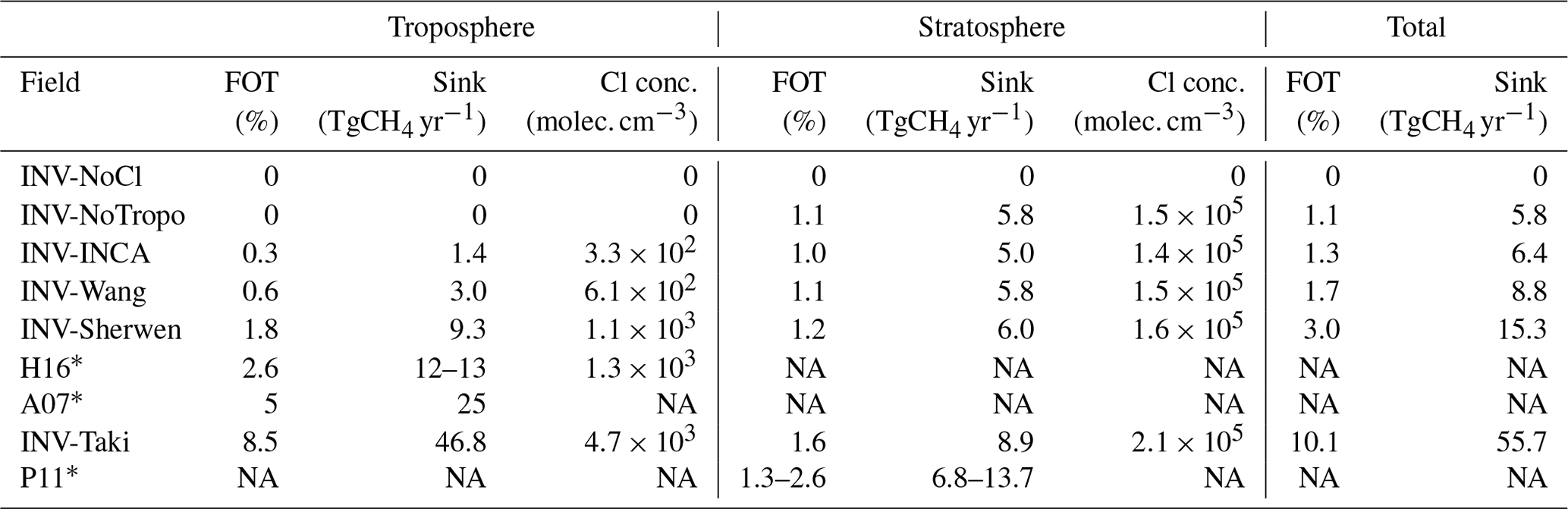
Note: NA is for not available. * Values taken from the literature, where H16 is from Hossaini et al. (2016), A07 is from Allan et al. (2007), and P11 is from Patra et al. (2011)
3.2 Spatial distributions of biases
Figure 2 shows the CH4 and δ13C(CH4) surface absolute biases between the simulations and the FWD-Wang averaged over the period 2010–2018. For CH4, globally averaged biases range from −18 to 123 ppb because prescribed Cl sinks are distinct. However, the spatial variations in biases around their mean value are similar for FWD-Taki, FWD-INCA, and FWD-Sherwen, since all the fields exhibit similar spatial patterns. For all biases, the minimum–maximum relative difference is below 5 %. Some biases are low enough for us to see the influence of surface fluxes (local CH4 enhancements) on biases in Fig. 2 (blue tropical regions in FWD-INCA and FWD-NoTropo panels). This is not visible in the bias corresponding to FWD-Sherwen and FWD-Taki, as the minimum–maximum difference is larger. Tropospheric Cl concentrations are generally larger in the tropics, and therefore, the bias between FWD-NoTropo and FWD-Wang is also larger in this latitudinal band. However, further removing the stratospheric Cl (FWD-NoCl) inverts the spatial distribution of the bias, hence leading to higher values in the polar regions. Following the Brewer–Dobson circulation, stratospheric air descends into the troposphere and mainly in polar regions (Butchart, 2014). The influence of stratospheric Cl on tropospheric CH4 mole fractions is therefore enhanced in these regions. To summarize, although spatial variations exist and can be slightly different from one field to another, they generally remain below 1 ppb and can be neglected.

Figure 2Surface absolute bias between FWD-* and FWD-Wang simulations averaged over 2010–2018. Temporal averaging is performed before substraction. The left column displays the biases between the CH4 mole fractions. The right column shows the biases between the δ13C(CH4) values. Note that the scales are different for each panel.
As for δ13C(CH4), globally averaged biases are larger than the recent global decline in δ13C(CH4) that has been observed since 2007 (Nisbet et al., 2019). Although mean values highly differ from one simulation to another, spatial variations are very similar, and we find the lowest values where the sources with the most depleted isotopic source signatures are located, e.g., in boreal regions (wetlands) and in Asia (agriculture and waste). These spatial discrepancies are likely caused by the nonlinear effects associated with isotopes. In a very simple framework, we can demonstrate that the steady-state bias Δδa between two simulations prescribing the same CH4 source and the same source signature δs is given by the following formula:
Δϵ denotes the difference in the prescribed fractionation between the two simulations due to differences in Cl concentrations. Note that the bias is dependent on the product of Δϵ and δs. More information and a comprehensive demonstration are provided in Sect. S4. Consequently, the bias will be lower if the source is more depleted in 13C. Figure 2 confirms that these nonlinear effects have a larger influence on the spatial patterns of the bias than stratospheric air intrusions, spatial differences between Cl concentrations, or even horizontal transport. In addition, the bias between FWD-NoTropo and FWD-NoCl is a good proxy for quantifying the influence of stratospheric Cl on δ13C(CH4) at the surface. At the end of the period, STEs cause a globally averaged increase in δ13C(CH4) at the surface of 0.30±0.01 ‰ (depending on the region) when the stratospheric Cl concentrations from Wang et al. (2021) are adopted. Although this value could change with another field, our range of stratospheric Cl concentrations is small, and the Cl-Wang field is taken from the most comprehensive and recent study to date. Therefore, we think that this value is a good estimate of the contemporary influence of stratospheric Cl on δ13C(CH4) at the surface. It is larger than the estimate of Wang et al. (2002) inferred between 1970 and 1992 (0.23 ‰). Both of our estimates were obtained after running a model for about the same number of years; therefore, these values are comparable. In addition, Wang et al. (2002) experimented with multiple configurations. In particular, one of the runs tested an enhanced STE, resulting in a value of 0.38 ‰. Another test, with stratospheric Cl concentrations increased by a factor 2, provided a value of 0.32 ‰. However, the latter study does not provide an estimate of the mean stratospheric Cl concentration. It is therefore difficult to know whether the discrepancy between both estimates is due to Cl stratospheric concentrations, the rate of STEs, or something else. Our value, however, lies within the full range obtained by Wang et al. (2002).
3.3 Global CH4 flux adjustment
The global CH4 flux adjustments resulting from a change in the Cl sink have been derived using the three methods introduced in Sect. 2.5 and are shown in Fig. 3. The INV-Wang simulation has been chosen as a reference. Global CH4 flux adjustments range from −7.0 Tg CH4 yr−1 (no Cl sink) to +46.8 Tg CH4 yr−1 (Cl-Taki) with M1. Small differences between M1 and the other methods exist (up to 10 %). However, the strong similarity between these results confirms that M2 and M3 can be employed to investigate the influence of the Cl sink on inversion-based adjustments for the global scale without significantly impacting the magnitude or sign of the results. This result, corresponding to Cl influence, may not be valid for larger changes such as those resulting from an OH sink modification. With the M1 method, more information about the spatial characteristics of the flux adjustment can be provided. About 70 % of the adjustment is made in the tropics (30∘ S–30∘ N) and the rest in the northern mid-latitudes (30–60∘ N). The other regions of the world contribute only to a few percent of the global adjustment. This is consistent with the spatial distribution of the biases presented in Sect. 3.2. Also, changing the reference scenario does not modify this distribution.

Figure 3Global CH4 flux and δ13C(CH4)source source signature adjustment due to a change in the prescribed Cl field. Panels (a) and (c) show the adjustments for the global CH4 flux (a) and δ13C(CH4)source source signature (c) with the multiple methods (M1, M2, and M3) presented in Sect. 2.5 and Sects. S1, S2 and S3. Simulations with Cl-Wang are taken as a reference. For M1 and M2, the error bars correspond to the interannual variations (1 standard deviation) of adjustments. Panels (b) and (d) display the linear model derived from the relationship between the adjustments (estimated with M1) and the mean tropospheric concentration of the prescribed Cl fields. For the linear regression only, simulations without the Cl sink (NoCl) are taken as a reference to calculate the adjustments.
Using this sample of results, we have also built a linear regression model in order to easily predict the influence of changing the Cl field on the global CH4 flux adjustment. By performing a linear regression between the adjustment values inferred with M1 and the mean tropospheric Cl concentrations, we obtain a coefficient of determination R2 very close to 1. It indicates that a linear relationship is a very good approximation of the relationship between the two variables. Consequently, one can affirm that each increase by 1000 in the mean tropospheric Cl concentration would require an adjustment of +11.7 Tg CH4 yr−1. It represents a change of about 2 % in the CH4 atmospheric oxidation, which is very small compared to the current uncertainties in OH sink intensity and their influences on top-down estimates (Zhao et al., 2020, 2019). Furthermore, the discrepancies between the mean tropospheric Cl concentrations estimated by recent studies are generally smaller than 1000 . Therefore, the uncertainty in CH4 emission estimates arising from the choice of Cl sink should not be larger than 11.7 Tg CH4 yr−1. However, inverse modelers should be extremely cautious before using Cl fields that exhibit much larger Cl concentrations than recent estimates. As shown here, it can cause the flux adjustment to reach 53.8 Tg CH4 yr−1.
As the inversion compensates for the sink difference induced by a change from one field (Cl-1) to another (Cl-2), the numerical value of the global flux adjustment is very close (less than a 10 % difference) to the difference between estimated tropospheric sink intensities for Cl-1 and Cl-2 (see Table 4). The stratospheric sink appears to have also a small influence on the results. For instance, between INV-NoCl and INV-NoTropo, there is a global flux adjustment of 3.8 Tg CH4 yr−1, resulting only from the difference in stratospheric Cl sink. It is significantly smaller than the stratospheric sink itself because a fraction of CH4 does not return to the troposphere from the stratosphere. In addition, stratospheric influence is not always the only cause of discrepancies. For instance, the global flux adjustment obtained with INV-Taki is 48.8±5.8 Tg CH4 yr−1, and the difference between the estimated total (tropospheric and stratospheric) sinks is 47.0±0.8 Tg CH4 yr−1. Therefore, differences between the estimated sinks alone cannot explain the global flux adjustment. It is very likely that if the spatial distributions of two tropospheric Cl sinks are different, then it can cause such discrepancies. Cl-Taki infers a larger proportion of its total sink in the tropics compared to Cl-Wang. However, the total chemical lifetime of CH4 is smaller in the tropics than in the high latitudes. Therefore, the inversion system must increase even more the CH4 flux in this region to compensate for these spatial distribution discrepancies. This effect remains, nevertheless, extremely small. For the other simulations, it is very difficult to separate the influence of the stratospheric sink from the influence of discrepancies arising from spatial distribution.
As the stratospheric Cl concentrations estimated by the models presented here suffer from much fewer uncertainties than the tropospheric Cl concentrations, we did not investigate the influence of the variations in stratospheric Cl. However, note that M2 and M3 have difficulties reproducing the M1 value when we remove the Cl sink entirely (NoCl bars in Fig. 3). It confirms that the stratospheric influence of Cl cannot be well captured by a box model framework.
3.4 Global δ13C(CH4)source source signature adjustment
Our methods are also designed to derive the global δ13C(CH4)source source signature adjustment resulting from a change in the prescribed Cl field. Figure 3 provides a comparison of the results with the three different methods. Global δ13C(CH4)source adjustments range from −4.1 ‰ (Cl-Taki) to +0.6 ‰ (no Cl sink) with M1. M2 and M3 results are highly consistent with M1 results, showing that simpler methods can also capture the δ13C(CH4)source adjustment. A linear regression model has also been built to quantify the relationship between the δ13C(CH4)source adjustment and the mean tropospheric Cl concentration. We obtain a coefficient of determination R2 very close to 1 and estimate that a δ13C(CH4)source adjustment of −1.0 ‰ would result from each increase by 1000 in the mean tropospheric Cl concentration to compensate for the enhanced atmospheric isotopic fractionation. Based on the Cl fields analyzed here, the globally averaged δ13C(CH4)source should very likely lie in the range of [−56.7, −51.9] ‰. If one excludes outliers, such as Cl-Taki or no Cl at all, then we deduce a likely range of [−53.1, −52.2] ‰ for the period 1998–2018. This range does not account for other uncertainties, e.g., uncertainties in the numerical value of the KIE associated with the OH sink.
We find a difference of 0.30 ‰ between the global δ13C(CH4)source inferred with INV-NoCl and INV-NoTropo, confirming the influence of stratospheric Cl on δ13C(CH4) at the surface first estimated in Sect. 3.2. This effect must be rigorously accounted for when using one-box modeling to estimate global CH4 emissions and dealing with isotopic constraints because it is comparable to the recent global decline in δ13C(CH4) that has been observed since 2007 (Nisbet et al., 2019). These results highlight that preferring one Cl field over another can highly influence the posterior globally averaged δ13C(CH4)source of an inversion performed with isotopic constraints. As the globally averaged δ13C(CH4)source mainly depends on the source mixture, contributions from emission categories to total emissions can be highly affected by a modification of the prescribed Cl field. In our inversions, WET, BB, FFG, and AGW emissions contribute between [32.5, 33.3] %, [4.9, 5.2] %, [21.0, 21.5] %, and [37.3, 37.6] %, respectively. For wetlands, such a variation roughly corresponds to a 15 Tg CH4 yr−1 change which results only from uncertainties in Cl concentrations. This adjustment is small compared to the wetland source uncertainty estimate of 41 Tg CH4 yr−1 for 2008–2017 derived by Saunois et al. (2020), albeit far from negligible. Furthermore, our inversions optimize the source signatures prescribed for each category and account for a relatively large uncertainty in prior estimates. Consequently, it releases part of the constraint that could be applied on the source mixture in an inversion not optimizing source signatures. Our results are therefore a lower-bound estimate of the influence of the Cl sink on top-down estimates with isotopic constraints. It emphasizes how careful one must be when selecting a prescribed Cl field for running such inversions.
3.5 CH4 and δ13C(CH4) seasonal cycles
The peak-to-peak amplitude of the CH4 seasonal cycle simulated by FWD-Wang at the surface typically ranges between 5 and 120 ppb, depending on the region (see Fig. S6 in the Supplement). It is larger where wetlands and biomass burning emissions are located because both sources exhibit a very strong seasonal dependence. Apart from the Cl-Taki field, changing the prescribed Cl field does not substantially modify the amplitude and the spatial variability in the CH4 seasonal cycle. Compared to FWD-Wang, the variation is below 3 % in both hemispheres for FWD-Sherwen, FWD-INCA, FWD-NoTropo, and FWD-NoCl. However, it can reach 10 % in the Northern Hemisphere when applying Cl-Taki instead of Cl-Wang.
As for δ13C(CH4), the seasonal cycle amplitude simulated by FWD-Wang typically ranges between 0.05 ‰ and 0.65 ‰. Again, changing the prescribed Cl field has more influence on δ13C(CH4) than on CH4. For instance, in the Southern Hemisphere, the variation in amplitude when switching from Cl-Wang to Cl-Sherwen is about 0.02 ‰, which represents 20 % of the total seasonal cycle amplitude. In the Northern Hemisphere, the variation can exceed 0.03 ‰, but it represents only 10 % of the seasonal cycle amplitude. Adopting the Cl-Taki field drastically increases this variation in the amplitude of the seasonal cycle, as variations can go up to 99 % in the Southern Hemisphere and 58 % in the Northern Hemisphere, with large spatial disparities. Also, differences in amplitudes for δ13C(CH4) between INV-NoTropo and INV-NoCl reach 10 % in the tropics and are negligible in other regions. It indicates that STE tends to slightly increase the seasonal cycle around the Equator when stratospheric Cl is included.
The influence of Cl on the simulated δ13C(CH4) seasonal cycle must be considered, as it impacts the results of an inversion with isotopic constraints. A misrepresentation of the seasonal cycle forces the system to adjust the intensity of sources that exert a large influence on the seasonal cycle, such as wetlands or biomass burning. Using the M1 method presented above, one can analyze the influence of prescribed Cl sink on optimized emissions for all categories. Apart from INV-Taki, the variation in the peak-to-peak amplitude of the seasonal cycle for global emissions and for each category is small between INV-Wang and all the other inverse configurations. It is below 5 % for WET, AGW, NAT, and FFG but can reach 10 % for BB. On the contrary, INV-Taki infers much larger-amplitude changes. The BB, WET, AGW, NAT, and FFG seasonal cycle amplitudes are increased by 3.1, 2.0, 0.1, 0.1, and 0.2 Tg CH4 yr−1 (134 %, 14 %, 9 %, 1 %, and 21 %), respectively.
3.6 CH4 vertical profiles
At present, vertical profile measurements of CH4 are too scarce to be considered to be a standalone constraint in inversion systems and so are rather used as evaluation data. Nevertheless, as their accuracy, spatial coverage, and number increase, their assimilation will become increasingly relevant. It is, however, necessary to increase the model–observation agreement, especially in the stratosphere, before considering their assimilation. We analyze here the influence of the Cl distribution on the simulated profiles. We also compare the simulated vertical profiles to observations to investigate whether modifying the Cl distribution can help to reduce the model-*observation discrepancies.
Simulated vertical profiles are sampled at the same locations and times as the available observations. Simulations with optimized fluxes (INV-*) are used to reduce the influence of a potential tropospheric bias resulting from a poor estimation of the CH4 fluxes and to analyze to what extent a station-based inversion can help to reduce both the tropospheric and stratospheric biases.
The bias bp between observed (obs) and simulated (sim) values for a specific profile p and for X= CH4 is given by the following:
We define the mean bias for a specific layer y (troposphere, or stratosphere) and a specific region of interest r as the root mean square difference (RMSD) over all the values of the bias in this layer and in this region.
Table 5RMSD between simulated and observed CH4 vertical profiles in the troposphere and stratosphere for different regions of the world.
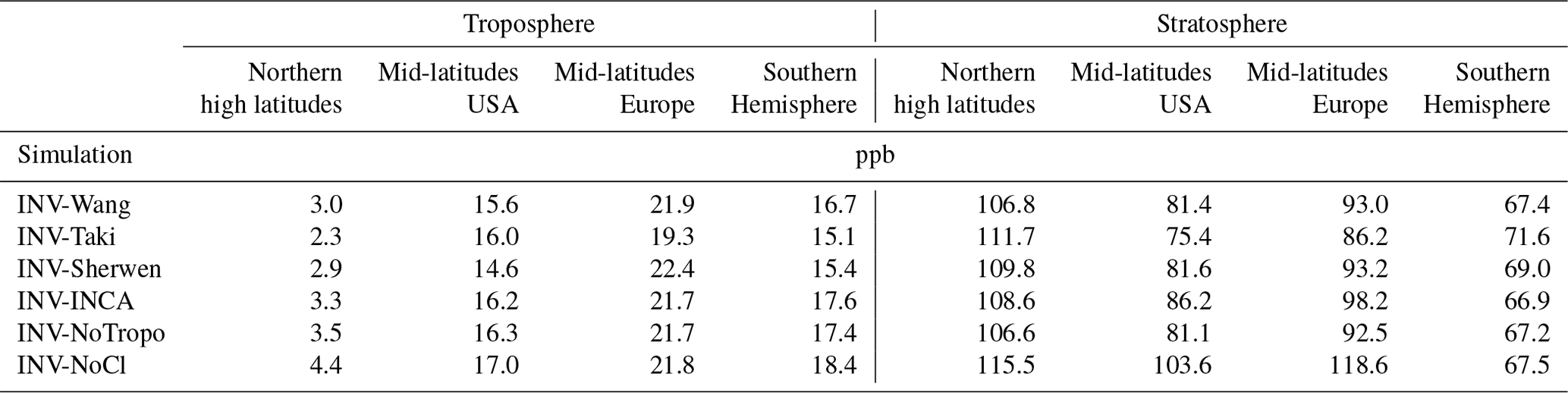
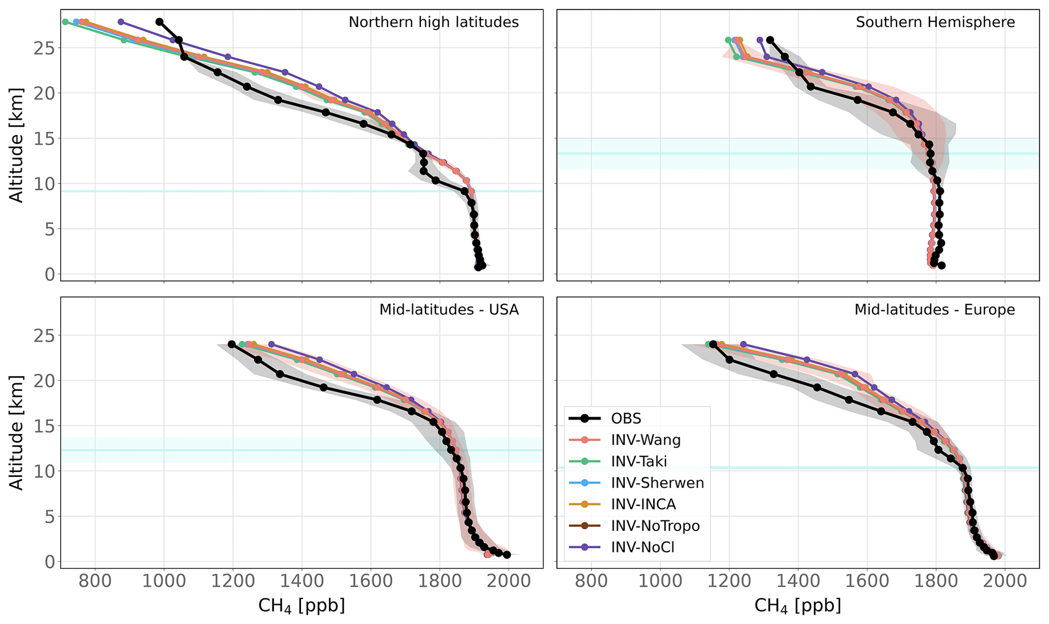
Figure 4Observed and simulated CH4 vertical profiles for four regions. All available vertical profiles in each region have been averaged. Shaded areas indicate the standard deviations of this average. The blue line and its associated shaded area show the mean altitude of the tropopause and its standard deviation over the vertical profiles in the region.
Table 5 shows the mean bias for four regions of the world where vertical profiles have been observed, i.e., the northern high latitudes in Europe, mid-latitudes in Europe, and mid-latitudes in the USA and Southern Hemisphere (Oceania). After inversion adjustments, tropospheric CH4 is well captured by the model. Biases are particularly low in the northern high latitudes, albeit the number of profiles (four) is much lower in this region, and additional data should be used to confirm this result. In the other regions, values are larger mainly because models have difficulties reproducing observed values very close to the surface. It is likely due to a problem of the representation of transport in the boundary layer in LMDz-SACS and/or a problem of the spatial representativity of sources that can be resolved only by increasing spatial resolution. Simulated profiles are generally slightly overestimated in Europe and underestimated in the USA in the troposphere, albeit by less than 10 ppb. Overall, the prescribed Cl field has very little impact on the tropospheric mean biases. Discrepancies between Cl fields for a given region are too small to validate one Cl field over another.
Mean biases are much larger in the stratosphere, ranging from about 67 ppb in the southern high latitudes to 115 ppb in the northern high latitudes. Outside the northern high latitudes, simulated values are generally larger than observed values for all simulations and all regions, showing that the model tends to overestimate CH4 mole fractions, even with optimized fluxes. Influences of the Cl sink are larger in the stratosphere for the four regions. INV-NoCl has more difficulties reproducing the simulated mole fractions above the tropopause, mainly in the Northern Hemisphere, with a mean bias that is 1.0 to 1.4 times larger than the other simulations. INV-Taki shows the lowest biases in the mid-latitudes, indicating that the stratospheric Cl concentrations could be underestimated in most of the tested fields in this region. However, this overestimation of CH4 mole fractions in the stratosphere could be also caused by an underestimation of the stratospheric OH or O(1D) concentrations or a weak transport between the troposphere and stratosphere, preventing the tropospheric CH4 from reaching higher altitudes. Such a misrepresentation may result in an overestimation of the column-weighted average mixing ratio (XCH4) simulated by LMDz-SACS (Ostler et al., 2016). An analysis of XCH4 is, however, beyond the scope of this study. Overall, modifying the Cl field has a very limited impact on simulated CH4 vertical profiles, as long as its stratospheric concentrations remain in the range analyzed here.
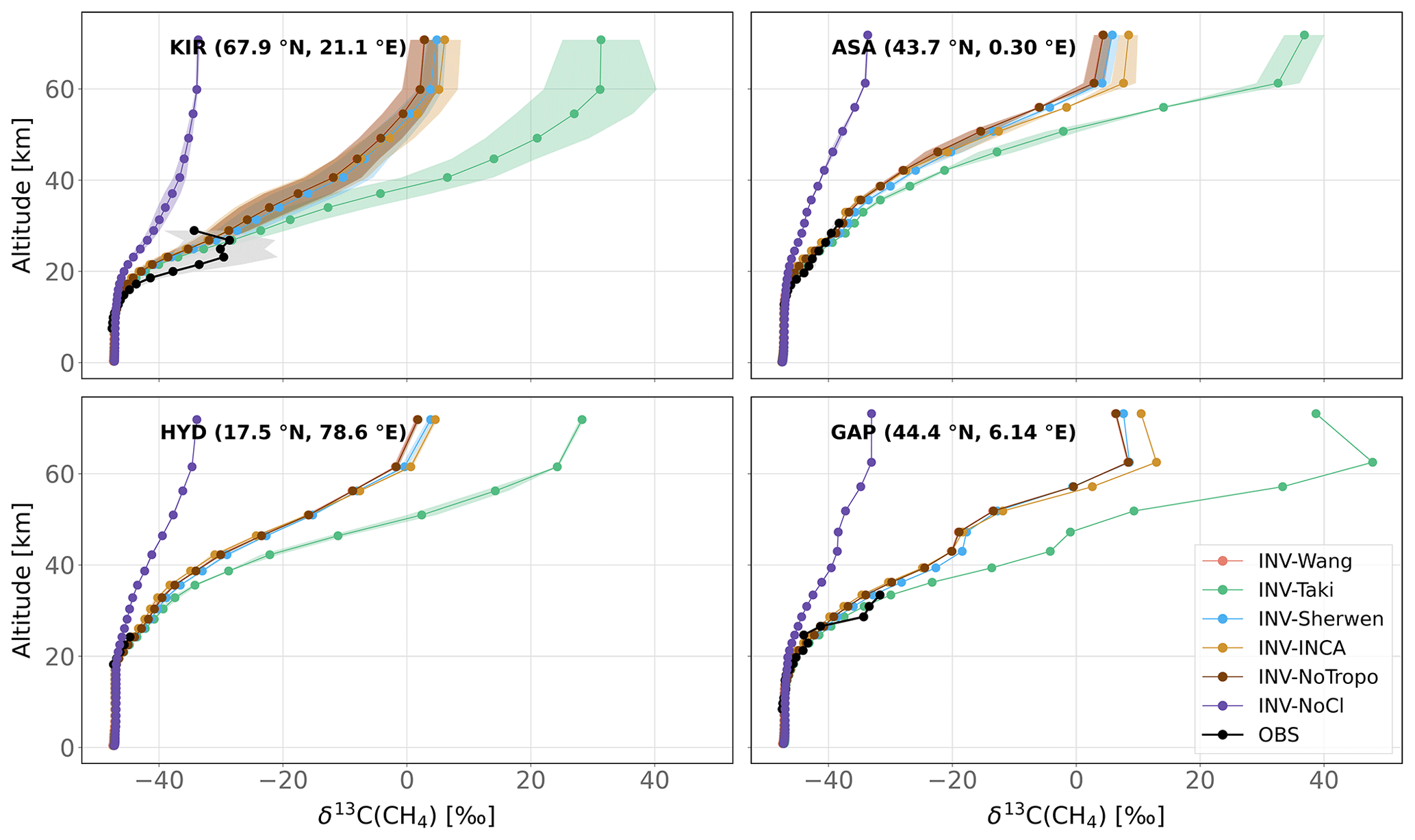
Figure 5Observed and simulated δ13C(CH4) vertical profiles for four locations. All available vertical profiles in each region have been averaged. Shaded areas indicate the standard deviations of this average. Note that measurement uncertainties (around 0.2 ‰) are much lower than the x axis range. KIR is Kiruna, Sweden (67.9∘ N, 21.10∘ E), ASA is Aire-sur-l'Adour, France (43.70∘ N, 0.30∘ E), HYD is Hyderabad, India (17.5∘ N, 78.60∘ E), and GAP is Gap, France (44.44∘ N, 6.14∘ E).
3.7 δ13C(CH4) vertical profiles
Figure 5 displays the comparison between observed vertical profiles of δ13C(CH4) from Röckmann et al. (2011) and those simulated by the INV-* runs. As most of the observed profiles were retrieved before the beginning of our simulations, we selected the year 2005 for the comparison. Although our inversions did optimize initial conditions, constraints from surface stations do not carry enough information to efficiently optimize the stratospheric δ13C(CH4). Therefore, a stabilization period in response to the prescribed Cl sink is necessary. However, in the stratosphere, this stabilization is somehow very fast (about 2–3 years), and the year selected for comparison has a negligible influence on the analysis. Selecting 1998 or 1999 slightly influences the comparison but does not affect the conclusions.
Apart from INV-NoCl, our simulations capture the observed profiles well. Vertical profiles of δ13C(CH4) that are simulated without any Cl sink are the most inconsistent with available observations. RMSDs of INV-NoCl over KIR (Kiruna, Sweden), ASA (Aire-sur-l'Adour, France), and GAP (Gap, France) are, respectively, 1.5, 2.2, and 2.5 times higher than the mean RMSD over the other simulations and over the same locations. Furthermore, the differences between Cl-INCA, Cl-Sherwen, and Cl-Wang have little influence on the vertical profiles of δ13C(CH4) due to the fact that the stratospheric Cl concentrations are relatively close (1.4–1.6×10⁵ ). Vertical profiles are well captured up to 30–35 km for ASA, HYD (Hyderabad, India), and GAP, confirming that the prescribed Cl concentrations in the lower stratosphere are realistic (average RMSDs of 1.0 ‰, 0.5 ‰, and 1.5 ‰). Cl-Taki stratospheric concentrations are slightly larger than the others, and therefore, simulated δ13C(CH4) is higher above 30–35 km for all regions.
Above KIR, in the polar regions, the simulated values are less consistent with observations (mean RMSD of 4.2 ‰). Several explanations can be given. First, current estimates of Cl concentrations may be underestimated in the lower stratosphere and in the polar regions. Second, the transport between the lower and upper stratosphere may not be correctly represented in the LMDz model, leading to a poor mixing between layers above the tropopause with 13C-enriched CH4 and more depleted layers below the tropopause. However, there is a high variability in the seven profiles analyzed above KIR (light gray band), and the simulated values are within the uncertainty in these observations. Overall, available observations are limited to approximately 30 km, and the influence of the prescribed Cl sink on the simulations is much clearer above this altitude. It is therefore difficult to prefer one Cl field over another without observing at higher altitudes.
In this study, we tested a large range of Cl concentration fields in order to investigate the influence of the Cl distribution on CH4 and δ13C(CH4) and to estimate its potential impact on the estimation of CH4 sources and isotopic signatures with top-down approaches. The Cl fields tested here are responsible for between 0.3 % and 8.5 % of the total CH4 sink in the troposphere and between 1.0 % and 1.6 % in the stratosphere. The differences in prescribed Cl concentrations lead to biases in simulated CH4 mole fractions and δ13C(CH4) isotopic composition that increase over time but stabilize after several decades.
We develop three methods to predict how an inversion system would adjust global emissions and source signatures in order to compensate for these CH4 and δ13C(CH4) biases. The most robust method (M1) provides flux adjustments ranging from −7.0 (no Cl sink) to +46.8 Tg CH4 yr−1 (Cl-Taki). The two other methods yield similar ranges. We show that these adjustment values linearly depend on tropospheric Cl concentrations and that each increase by 1000 in the mean tropospheric Cl concentration would require an adjustment of +11.7 Tg CH4 yr−1. However, most of the fields tested here lead to an adjustment below 10 Tg CH4 yr−1. It therefore remains small in comparison to the uncertainties inferred by Saunois et al. (2020).
The same method is applied to quantify the globally averaged δ13C(CH4)source adjustment. We also find a good linear relationship between the adjustment and the mean tropospheric Cl concentration. A source signature adjustment of −1.0 ‰ would therefore result from an increase of 1000 in the mean tropospheric Cl concentration to compensate for the enhanced atmospheric isotopic fractionation. After discarding the Cl-Taki field and the possibility of neglecting the Cl sink, we estimate that the globally averaged source signature ranges from −53.1 ‰ to −52.2 ‰. This range represents the uncertainty in the globally averaged source signature resulting from uncertainties in tropospheric Cl concentrations. However, it does not account for other uncertainties, e.g., those related to the KIE of the OH sink. Also, we find that intrusions of stratospheric air are responsible for an enrichment of δ13C(CH4) by 0.30 ‰ at the surface in comparison with an atmosphere without stratospheric Cl. We also show here that the choice of the Cl field has a very strong influence on the source mixture obtained with an inversion assimilating δ13C(CH4) observations.
A modification of the Cl field within the tested range only slightly influences CH4 seasonal cycles. It can nevertheless modify the amplitudes of the δ13C(CH4) seasonal cycle by up to 10 %–20 % for most of the tested fields, depending on the latitude. To compensate for this change in the seasonal cycles, an inversion system might reduce or amplify the seasonal cycles of each emission categories, in particular those which have a large impact on the δ13C(CH4) seasonal cycle, namely wetlands and biomass burning.
We also investigate the influence of Cl concentrations on the modeling of CH4 and δ13C(CH4) vertical profiles. Observed profiles are well captured by the model, although simulated CH4 mole fractions are generally larger than observed values above the tropopause. We conclude that these discrepancies in LMDz-SACS are unlikely to be caused by a misrepresentation of the Cl sink.
It is difficult to conclude which Cl field provides the most realistic representation of the Cl sink among those tested here. Recent developments and efforts have nevertheless narrowed the range of uncertainties regarding the Cl concentrations (less than 1.1×10³ in the troposphere and 1.4–1.6×10⁵ in the stratosphere). Our study shows that the impact of a change in Cl field on top-down CH4 flux estimates should be small compared to current uncertainties in Saunois et al. (2020) if this change is made within the range of Cl concentrations recently estimated. A Cl distribution for all inversions agreed upon in multi-model studies, such as Saunois et al. (2020), should reduce the spread in estimated CH4 fluxes. We suggest adopting recent estimates, especially those of Wang et al. (2021), which result from the most comprehensive study to date.
The data for CH4 (https://doi.org/10.15138/VNCZ-M766, Lan et al., 2022) and δ13C(CH4) observations were downloaded from the NOAA-ESRL server https://www.esrl.noaa.gov/gmd/aftp/data/trace_gases (White et al., 2021). Data sets for the input emissions were provided by the Global Carbon Project (GCP) team. The AirCore vertical profiles from the NOAA-ESRL Aircraft Program (https://doi.org/10.15138/6AV0-MY81; version 20181101; Baier et al., 2021) were provided by Colm Sweeney and Bianca Baier. The Cl-Sherwen and Cl-Wang fields were provided by the corresponding authors of Sherwen et al. (2016b) and Wang et al. (2021), respectively. The Cl-INCA field, the modeling output files, and the AirCore vertical profiles from the French AirCore Program are available, upon request, from the corresponding author.
The supplement related to this article is available online at: https://doi.org/10.5194/acp-22-15489-2022-supplement.
JT designed and ran the simulation experiments and performed the data analysis presented in this paper. DH provided the Cl-INCA field used for the simulations. MS provided the CH4 fluxes. CS and BB provided the AirCore vertical profiles from the NOAA/ESRL Aircraft Program. MS, AB, IP, and PB provided scientific, technical expertise and contributed to the scientific analysis of this work. JT prepared the paper, with contributions from all co-authors.
The contact author has declared that none of the authors has any competing interests.
Publisher's note: Copernicus Publications remains neutral with regard to jurisdictional claims in published maps and institutional affiliations.
This work has been supported by the CEA (Commissariat à l'Energie Atomique et aux Energies Alternatives). The study extensively relies on the meteorological data provided by the ECMWF. Calculations were performed using the computing resources of LSCE, which are maintained by François Marabelle and the LSCE IT team. The authors wish to thank the measurement teams from the NOAA GML and from INSTAAR for their work. Finally, the authors thank all the referees, for their fruitful comments and suggestions on the paper.
This research has been supported by the Commissariat à l'Energie Atomique et aux Energies Alternatives (grant no. CFR 2018).
This paper was edited by Andreas Hofzumahaus and reviewed by five anonymous referees.
Allan, W., Struthers, H., and Lowe, D. C.: Methane carbon isotope effects caused by atomic chlorine in the marine boundary layer: Global model results compared with Southern Hemisphere measurements, J. Geophys. Res., 112, D04306, https://doi.org/10.1029/2006JD007369, 2007. a, b, c, d, e, f, g, h, i, j
Baier, B., Sweeney, C., Tans, P., Newberger, T., Higgs, J., Wolter, S., and NOAA Global Monitoring Laboratory: NOAA AirCore atmospheric sampling system profiles (Version 20210813), NOAA GML [data set], https://doi.org/10.15138/6AV0-MY81, 2021. a, b
Berchet, A., Sollum, E., Thompson, R. L., Pison, I., Thanwerdas, J., Broquet, G., Chevallier, F., Aalto, T., Berchet, A., Bergamaschi, P., Brunner, D., Engelen, R., Fortems-Cheiney, A., Gerbig, C., Groot Zwaaftink, C. D., Haussaire, J.-M., Henne, S., Houweling, S., Karstens, U., Kutsch, W. L., Luijkx, I. T., Monteil, G., Palmer, P. I., van Peet, J. C. A., Peters, W., Peylin, P., Potier, E., Rödenbeck, C., Saunois, M., Scholze, M., Tsuruta, A., and Zhao, Y.: The Community Inversion Framework v1.0: a unified system for atmospheric inversion studies, Geosci. Model Dev., 14, 5331–5354, https://doi.org/10.5194/gmd-14-5331-2021, 2021. a
Bousquet, P., Ciais, P., Miller, J. B., Dlugokencky, E. J., Hauglustaine, D. A., Prigent, C., Van der Werf, G. R., Peylin, P., Brunke, E.-G., Carouge, C., Langenfelds, R. L., Lathière, J., Papa, F., Ramonet, M., Schmidt, M., Steele, L. P., Tyler, S. C., and White, J.: Contribution of anthropogenic and natural sources to atmospheric methane variability, Nature, 443, 439–443, https://doi.org/10.1038/nature05132, 2006. a
Burkholder, J. B., Abbatt, J. P. D., Huie, R. E., Kurylo, M. J., Wilmouth, D. M., Sander, S. P., Barker, J. R., Kolb, C. E., Orkin, V. L., and Wine, P. H.: JPL Publication 15-10: Chemical Kinetics and Photochemical Data for Use in Atmospheric Studies, p. 1392, 2015. a
Butchart, N.: The Brewer-Dobson circulation, Rev. Geophys., 52, 157–184, https://doi.org/10.1002/2013RG000448, 2014. a
Cantrell, C. A., Shetter, R. E., McDaniel, A. H., Calvert, J. G., Davidson, J. A., Lowe, D. C., Tyler, S. C., Cicerone, R. J., and Greenberg, J. P.: Carbon kinetic isotope effect in the oxidation of methane by the hydroxyl radical, J. Geophys. Res.-Atmos., 95, 22455–22462, https://doi.org/10.1029/JD095iD13p22455, 1990. a
Chevallier, F., Fisher, M., Peylin, P., Serrar, S., Bousquet, P., Bréon, F.-M., Chédin, A., and Ciais, P.: Inferring CO2 sources and sinks from satellite observations: Method and application to TOVS data, J. Geophys. Res., 110, D24309, https://doi.org/10.1029/2005JD006390, 2005. a
Craig, H.: Isotopic standards for carbon and oxygen and correction factors for mass-spectrometric analysis of carbon dioxide, Geochim. Cosmochim. Ac., 12, 133–149, https://doi.org/10.1016/0016-7037(57)90024-8, 1957. a
Dlugokencky, E. J.: NOAA/GML, http://www.esrl.noaa.gov/gmd/ccgg/trends_ch4/, last access: 9 May 2022. a, b
Etheridge, D. M., Steele, L. P., Francey, R. J., and Langenfelds, R. L.: Atmospheric methane between 1000 A.D. and present: Evidence of anthropogenic emissions and climatic variability, J. Geophys. Res.-Atmos., 103, 15979–15993, https://doi.org/10.1029/98JD00923, 1998. a
Fletcher, S. E. M., Tans, P. P., Bruhwiler, L. M., Miller, J. B., and Heimann, M.: CH4 sources estimated from atmospheric observations of CH4 and its 13C/12C isotopic ratios: 2. Inverse modeling of CH4 fluxes from geographical regions, Global Biogeochem. Cycles, 18, GB4005, https://doi.org/10.1029/2004GB002224, 2004. a
Folberth, G. A., Hauglustaine, D. A., Lathière, J., and Brocheton, F.: Interactive chemistry in the Laboratoire de Météorologie Dynamique general circulation model: model description and impact analysis of biogenic hydrocarbons on tropospheric chemistry, Atmos. Chem. Phys., 6, 2273–2319, https://doi.org/10.5194/acp-6-2273-2006, 2006. a
Fujita, R., Morimoto, S., Maksyutov, S., Kim, H.-S., Arshinov, M., Brailsford, G., Aoki, S., and Nakazawa, T.: Global and Regional CH4 Emissions for 1995–2013 Derived From Atmospheric CH4, δ13C-CH4, and δD-CH4 Observations and a Chemical Transport Model, J. Geophys. Res.-Atmos., 125, e2020JD032903, https://doi.org/10.1029/2020JD032903, 2020. a
Gromov, S., Brenninkmeijer, C. A. M., and Jöckel, P.: A very limited role of tropospheric chlorine as a sink of the greenhouse gas methane, Atmos. Chem. Phys., 18, 9831–9843, https://doi.org/10.5194/acp-18-9831-2018, 2018. a, b, c, d, e
Gupta, M., Tyler, S., and Cicerone, R.: Modeling atmospheric δ13CH4 and the causes of recent changes in atmospheric CH4 amounts, J. Geophys. Res.-Atmos., 101, 22923–22932, https://doi.org/10.1029/96JD02386, 1996. a
Hauglustaine, D. A., Hourdin, F., Jourdain, L., Filiberti, M.-A., Walters, S., Lamarque, J.-F., and Holland, E. A.: Interactive chemistry in the Laboratoire de Météorologie Dynamique general circulation model: Description and background tropospheric chemistry evaluation, J. Geophys. Res.-Atmos., 109, D04314, https://doi.org/10.1029/2003JD003957, 2004. a
Hauglustaine, D. A., Cozic, A., Caubel, A., Lathière, J., Sépulchre, P., Cohen, Y., Balkanski, Y., Lurton, T., Boucher, O., and Tsigaridis, K.: Coupled Climate-Chemistry-Aerosol simulations under the AerChemMIP scenarios with the IPSL-CM5A2-INCA climate model, in preparation, 2021. a, b
Hossaini, R., Chipperfield, M. P., Saiz-Lopez, A., Fernandez, R., Monks, S., Feng, W., Brauer, P., and von Glasow, R.: A global model of tropospheric chlorine chemistry: Organic versus inorganic sources and impact on methane oxidation, J. Geophys. Res.-Atmos., 121, 14271–14297, https://doi.org/10.1002/2016JD025756, 2016. a, b, c, d, e, f, g, h
Hourdin, F., Musat, I., Bony, S., Braconnot, P., Codron, F., Dufresne, J.-L., Fairhead, L., Filiberti, M.-A., Friedlingstein, P., Grandpeix, J.-Y., Krinner, G., LeVan, P., Li, Z.-X., and Lott, F.: The LMDZ4 general circulation model: climate performance and sensitivity to parametrized physics with emphasis on tropical convection, Clim. Dynam., 27, 787–813, https://doi.org/10.1007/s00382-006-0158-0, 2006. a
Houweling, S., Bergamaschi, P., Chevallier, F., Heimann, M., Kaminski, T., Krol, M., Michalak, A. M., and Patra, P.: Global inverse modeling of CH4 sources and sinks: an overview of methods, Atmos. Chem. Phys., 17, 235–256, https://doi.org/10.5194/acp-17-235-2017, 2017. a
Karion, A., Sweeney, C., Tans, P., and Newberger, T.: AirCore: An Innovative Atmospheric Sampling System, J. Atmos. Ocean. Tech., 27, 1839–1853, https://doi.org/10.1175/2010JTECHA1448.1, 2010. a, b
Lan, X., Dlugokencky, E. J., Mund, J. W., Crotwell, A. M., Crotwell, M. J., Moglia, E., Madronich, M., Neff, D., and Thoning, K. W.: Atmospheric Methane Dry Air Mole Fractions from the NOAA GML Carbon Cycle Cooperative Global Air Sampling Network, 1983–2021, Version: 2022-11-21, NOAA Global Monitoring Laboratory Data Repository [data set], https://doi.org/10.15138/VNCZ-M766, 2022. a
Locatelli, R., Bousquet, P., Hourdin, F., Saunois, M., Cozic, A., Couvreux, F., Grandpeix, J.-Y., Lefebvre, M.-P., Rio, C., Bergamaschi, P., Chambers, S. D., Karstens, U., Kazan, V., van der Laan, S., Meijer, H. A. J., Moncrieff, J., Ramonet, M., Scheeren, H. A., Schlosser, C., Schmidt, M., Vermeulen, A., and Williams, A. G.: Atmospheric transport and chemistry of trace gases in LMDz5B: evaluation and implications for inverse modelling, Geosci. Model Dev., 8, 129–150, https://doi.org/10.5194/gmd-8-129-2015, 2015. a
Louis, J.-F.: A parametric model of vertical eddy fluxes in the atmosphere, Bound.-Lay. Meteorol., 17, 187–202, https://doi.org/10.1007/BF00117978, 1979. a
Mailler, S., Menut, L., Khvorostyanov, D., Valari, M., Couvidat, F., Siour, G., Turquety, S., Briant, R., Tuccella, P., Bessagnet, B., Colette, A., Létinois, L., Markakis, K., and Meleux, F.: CHIMERE-2017: from urban to hemispheric chemistry-transport modeling, Geosci. Model Dev., 10, 2397–2423, https://doi.org/10.5194/gmd-10-2397-2017, 2017. a
McCarthy, M. C., Connell, P., and Boering, K. A.: Isotopic fractionation of methane in the stratosphere and its effect on free tropospheric isotopic compositions, Geophys. Res. Lett., 28, 3657–3660, https://doi.org/10.1029/2001GL013159, 2001. a
McCarthy, M. C., Boering, K. A., Rice, A. L., Tyler, S. C., Connell, P., and Atlas, E.: Carbon and hydrogen isotopic compositions of stratospheric methane: 2. Two-dimensional model results and implications for kinetic isotope effects, J. Geophys. Res.-Atmos., 108, 4461, https://doi.org/10.1029/2002JD003183, 2003. a, b, c, d
McNorton, J., Wilson, C., Gloor, M., Parker, R. J., Boesch, H., Feng, W., Hossaini, R., and Chipperfield, M. P.: Attribution of recent increases in atmospheric methane through 3-D inverse modelling, Atmos. Chem. Phys., 18, 18149–18168, https://doi.org/10.5194/acp-18-18149-2018, 2018. a, b
Meinshausen, M., Vogel, E., Nauels, A., Lorbacher, K., Meinshausen, N., Etheridge, D. M., Fraser, P. J., Montzka, S. A., Rayner, P. J., Trudinger, C. M., Krummel, P. B., Beyerle, U., Canadell, J. G., Daniel, J. S., Enting, I. G., Law, R. M., Lunder, C. R., O'Doherty, S., Prinn, R. G., Reimann, S., Rubino, M., Velders, G. J. M., Vollmer, M. K., Wang, R. H. J., and Weiss, R.: Historical greenhouse gas concentrations for climate modelling (CMIP6), Geosci. Model Dev., 10, 2057–2116, https://doi.org/10.5194/gmd-10-2057-2017, 2017. a
Membrive, O., Crevoisier, C., Sweeney, C., Danis, F., Hertzog, A., Engel, A., Bönisch, H., and Picon, L.: AirCore-HR: a high-resolution column sampling to enhance the vertical description of CH4 and CO2, Atmos. Meas. Tech., 10, 2163–2181, https://doi.org/10.5194/amt-10-2163-2017, 2017. a
Menut, L., Bessagnet, B., Khvorostyanov, D., Beekmann, M., Blond, N., Colette, A., Coll, I., Curci, G., Foret, G., Hodzic, A., Mailler, S., Meleux, F., Monge, J.-L., Pison, I., Siour, G., Turquety, S., Valari, M., Vautard, R., and Vivanco, M. G.: CHIMERE 2013: a model for regional atmospheric composition modelling, Geosci. Model Dev., 6, 981–1028, https://doi.org/10.5194/gmd-6-981-2013, 2013. a
Monteil, G., Houweling, S., Dlugockenky, E. J., Maenhout, G., Vaughn, B. H., White, J. W. C., and Rockmann, T.: Interpreting methane variations in the past two decades using measurements of CH4 mixing ratio and isotopic composition, Atmos. Chem. Phys., 11, 9141–9153, https://doi.org/10.5194/acp-11-9141-2011, 2011. a
Müller, R., Brenninkmeijer, C. A. M., and Crutzen, P. J.: A large 13CO deficit in the lower Antarctic stratosphere due to “ozone hole” chemistry: Part II, Modeling, Geophys. Res. Lett., 23, 2129–2132, https://doi.org/10.1029/96GL01472, 1996. a
Neef, L., Weele, M. V., and Velthoven, P. V.: Optimal estimation of the present-day global methane budget, Global Biogeochem. Cycles, 24, GB4024, https://doi.org/10.1029/2009GB003661, 2010. a
Nisbet, E. G., Manning, M. R., Dlugokencky, E. J., Fisher, R. E., Lowry, D., Michel, S. E., Myhre, C. L., Platt, S. M., Allen, G., Bousquet, P., Brownlow, R., Cain, M., France, J. L., Hermansen, O., Hossaini, R., Jones, A. E., Levin, I., Manning, A. C., Myhre, G., Pyle, J. A., Vaughn, B. H., Warwick, N. J., and White, J. W. C.: Very Strong Atmospheric Methane Growth in the 4 Years 2014–2017: Implications for the Paris Agreement, Global Biogeochemical Cycles, 33, 318–342, https://doi.org/10.1029/2018GB006009, 2019. a, b, c, d
Ostler, A., Sussmann, R., Patra, P. K., Houweling, S., De Bruine, M., Stiller, G. P., Haenel, F. J., Plieninger, J., Bousquet, P., Yin, Y., Saunois, M., Walker, K. A., Deutscher, N. M., Griffith, D. W. T., Blumenstock, T., Hase, F., Warneke, T., Wang, Z., Kivi, R., and Robinson, J.: Evaluation of column-averaged methane in models and TCCON with a focus on the stratosphere, Atmos. Meas. Tech., 9, 4843–4859, https://doi.org/10.5194/amt-9-4843-2016, 2016. a
Patra, P. K., Houweling, S., Krol, M., Bousquet, P., Belikov, D., Bergmann, D., Bian, H., Cameron-Smith, P., Chipperfield, M. P., Corbin, K., Fortems-Cheiney, A., Fraser, A., Gloor, E., Hess, P., Ito, A., Kawa, S. R., Law, R. M., Loh, Z., Maksyutov, S., Meng, L., Palmer, P. I., Prinn, R. G., Rigby, M., Saito, R., and Wilson, C.: TransCom model simulations of CH4 and related species: linking transport, surface flux and chemical loss with CH4 variability in the troposphere and lower stratosphere, Atmos. Chem. Phys., 11, 12813–12837, https://doi.org/10.5194/acp-11-12813-2011, 2011. a, b, c, d
Pison, I., Bousquet, P., Chevallier, F., Szopa, S., and Hauglustaine, D.: Multi-species inversion of CH4, CO and H2 emissions from surface measurements, Atmos. Chem. Phys., 9, 5281–5297, https://doi.org/10.5194/acp-9-5281-2009, 2009. a, b
Rice, A. L., Tyler, S. C., McCarthy, M. C., Boering, K. A., and Atlas, E.: Carbon and hydrogen isotopic compositions of stratospheric methane: 1. High-precision observations from the NASA ER-2 aircraft, J. Geophys. Res.-Atmos., 108, 4460, https://doi.org/10.1029/2002JD003042, 2003. a
Rice, A. L., Butenhoff, C. L., Teama, D. G., Röger, F. H., Khalil, M. A. K., and Rasmussen, R. A.: Atmospheric methane isotopic record favors fossil sources flat in 1980s and 1990s with recent increase, P. Natl. Acad. Sci. USA, 113, 10791–10796, https://doi.org/10.1073/pnas.1522923113, 2016. a
Rigby, M., Manning, A. J., and Prinn, R. G.: The value of high-frequency, high-precision methane isotopologue measurements for source and sink estimation, J. Geophys. Res.-Atmos., 117, D12312, https://doi.org/10.1029/2011JD017384, 2012. a
Röckmann, T., Grooß, J.-U., and Müller, R.: The impact of anthropogenic chlorine emissions, stratospheric ozone change and chemical feedbacks on stratospheric water, Atmos. Chem. Phys., 4, 693–699, https://doi.org/10.5194/acp-4-693-2004, 2004. a
Röckmann, T., Brass, M., Borchers, R., and Engel, A.: The isotopic composition of methane in the stratosphere: high-altitude balloon sample measurements, Atmos. Chem. Phys., 11, 13287–13304, https://doi.org/10.5194/acp-11-13287-2011, 2011. a, b
Saueressig, G., Bergamaschi, P., Crowley, J. N., Fischer, H., and Harris, G. W.: Carbon kinetic isotope effect in the reaction of CH4 with Cl atoms, Geophys. Res. Lett., 22, 1225–1228, https://doi.org/10.1029/95GL00881, 1995. a
Saueressig, G., Crowley, J. N., Bergamaschi, P., Brühl, C., Brenninkmeijer, C. A. M., and Fischer, H.: Carbon 13 and D kinetic isotope effects in the reactions of CH4 with O(1D) and OH: New laboratory measurements and their implications for the isotopic composition of stratospheric methane, J. Geophys. Res.-Atmos., 106, 23127–23138, https://doi.org/10.1029/2000JD000120, 2001. a, b, c, d, e
Saunois, M., Stavert, A. R., Poulter, B., Bousquet, P., Canadell, J. G., Jackson, R. B., Raymond, P. A., Dlugokencky, E. J., Houweling, S., Patra, P. K., Ciais, P., Arora, V. K., Bastviken, D., Bergamaschi, P., Blake, D. R., Brailsford, G., Bruhwiler, L., Carlson, K. M., Carrol, M., Castaldi, S., Chandra, N., Crevoisier, C., Crill, P. M., Covey, K., Curry, C. L., Etiope, G., Frankenberg, C., Gedney, N., Hegglin, M. I., Höglund-Isaksson, L., Hugelius, G., Ishizawa, M., Ito, A., Janssens-Maenhout, G., Jensen, K. M., Joos, F., Kleinen, T., Krummel, P. B., Langenfelds, R. L., Laruelle, G. G., Liu, L., Machida, T., Maksyutov, S., McDonald, K. C., McNorton, J., Miller, P. A., Melton, J. R., Morino, I., Müller, J., Murguia-Flores, F., Naik, V., Niwa, Y., Noce, S., O'Doherty, S., Parker, R. J., Peng, C., Peng, S., Peters, G. P., Prigent, C., Prinn, R., Ramonet, M., Regnier, P., Riley, W. J., Rosentreter, J. A., Segers, A., Simpson, I. J., Shi, H., Smith, S. J., Steele, L. P., Thornton, B. F., Tian, H., Tohjima, Y., Tubiello, F. N., Tsuruta, A., Viovy, N., Voulgarakis, A., Weber, T. S., van Weele, M., van der Werf, G. R., Weiss, R. F., Worthy, D., Wunch, D., Yin, Y., Yoshida, Y., Zhang, W., Zhang, Z., Zhao, Y., Zheng, B., Zhu, Q., Zhu, Q., and Zhuang, Q.: The Global Methane Budget 2000–2017, Earth Syst. Sci. Data, 12, 1561–1623, https://doi.org/10.5194/essd-12-1561-2020, 2020. a, b, c, d, e, f, g, h, i, j, k, l, m
Schaefer, H., Fletcher, S. E. M., Veidt, C., Lassey, K. R., Brailsford, G. W., Bromley, T. M., Dlugokencky, E. J., Michel, S. E., Miller, J. B., Levin, I., Lowe, D. C., Martin, R. J., Vaughn, B. H., and White, J. W. C.: A 21st-century shift from fossil-fuel to biogenic methane emissions indicated by 13CH4, Science, 352, 80–84, https://doi.org/10.1126/science.aad2705, 2016. a
Schwietzke, S., Sherwood, O. A., Bruhwiler, L. M. P., Miller, J. B., Etiope, G., Dlugokencky, E. J., Michel, S. E., Arling, V. A., Vaughn, B. H., White, J. W. C., and Tans, P. P.: Upward revision of global fossil fuel methane emissions based on isotope database, Nature, 538, 88–91, https://doi.org/10.1038/nature19797, 2016. a
Sherwen, T., Evans, M. J., Carpenter, L. J., Andrews, S. J., Lidster, R. T., Dix, B., Koenig, T. K., Sinreich, R., Ortega, I., Volkamer, R., Saiz-Lopez, A., Prados-Roman, C., Mahajan, A. S., and Ordóñez, C.: Iodine's impact on tropospheric oxidants: a global model study in GEOS-Chem, Atmos. Chem. Phys., 16, 1161–1186, https://doi.org/10.5194/acp-16-1161-2016, 2016a. a
Sherwen, T., Schmidt, J. A., Evans, M. J., Carpenter, L. J., Großmann, K., Eastham, S. D., Jacob, D. J., Dix, B., Koenig, T. K., Sinreich, R., Ortega, I., Volkamer, R., Saiz-Lopez, A., Prados-Roman, C., Mahajan, A. S., and Ordóñez, C.: Global impacts of tropospheric halogens (Cl, Br, I) on oxidants and composition in GEOS-Chem, Atmos. Chem. Phys., 16, 12239–12271, https://doi.org/10.5194/acp-16-12239-2016, 2016b. a, b, c, d, e, f, g, h
Sherwood, O. A., Schwietzke, S., Arling, V. A., and Etiope, G.: Global Inventory of Gas Geochemistry Data from Fossil Fuel, Microbial and Burning Sources, version 2017, Earth Syst. Sci. Data, 9, 639–656, https://doi.org/10.5194/essd-9-639-2017, 2017. a
Stolper, D. A., Sessions, A. L., Ferreira, A. A., Santos Neto, E. V., Schimmelmann, A., Shusta, S. S., Valentine, D. L., and Eiler, J. M.: Combined 13C–D and D–D clumping in methane: Methods and preliminary results, Geochim. Cosmochim. Ac., 126, 169–191, https://doi.org/10.1016/j.gca.2013.10.045, 2014. a
Strode, S. A., Wang, J. S., Manyin, M., Duncan, B., Hossaini, R., Keller, C. A., Michel, S. E., and White, J. W. C.: Strong sensitivity of the isotopic composition of methane to the plausible range of tropospheric chlorine, Atmos. Chem. Phys., 20, 8405–8419, https://doi.org/10.5194/acp-20-8405-2020, 2020. a
Takigawa, M., Takahashi, M., and Akiyoshi, H.: Simulation of ozone and other chemical species using a Center for Climate System Research/National Institute for Environmental Studies atmospheric GCM with coupled stratospheric chemistry, J. Geophys. Res.-Atmos., 104, 14003–14018, https://doi.org/10.1029/1998JD100105, 1999. a, b
Terrenoire, E., Hauglustaine, D. A., Cohen, Y., Cozic, A., Valorso, R., Lefèvre, F., and Matthes, S.: Impact of present and future aircraft NOx and aerosol emissions on atmospheric composition and associated direct radiative forcing of climate, Atmos. Chem. Phys., 22, 11987–12023, https://doi.org/10.5194/acp-22-11987-2022, 2022. a
Thanwerdas, J., Saunois, M., Berchet, A., Pison, I., Vaughn, B. H., Michel, S. E., and Bousquet, P.: Variational inverse modeling within the Community Inversion Framework v1.1 to assimilate δ13C(CH4) and CH4: a case study with model LMDz-SACS, Geosci. Model Dev., 15, 4831–4851, https://doi.org/10.5194/gmd-15-4831-2022, 2022. a, b, c, d, e
Thompson, R. L., Nisbet, E. G., Pisso, I., Stohl, A., Blake, D., Dlugokencky, E. J., Helmig, D., and White, J. W. C.: Variability in Atmospheric Methane From Fossil Fuel and Microbial Sources Over the Last Three Decades, Geophys. Res. Lett., 45, 11499–11508, https://doi.org/10.1029/2018GL078127, 2018. a
Tiedtke, M.: A Comprehensive Mass Flux Scheme for Cumulus Parameterization in Large-Scale Models, Mon. Weather Rev., 117, 1779–1800, https://doi.org/10.1175/1520-0493(1989)117<1779:ACMFSF>2.0.CO;2, 1989. a
Wang, J. S., McElroy, M. B., Spivakovsky, C. M., and Jones, D. B. A.: On the contribution of anthropogenic Cl to the increase in δ13C of atmospheric methane: ANTHROPOGENIC Cl AND δ13C OF METHANE, Global Biogeochem. Cycles, 16, 20-1–20-11, https://doi.org/10.1029/2001GB001572, 2002. a, b, c, d, e
Wang, X., Jacob, D. J., Eastham, S. D., Sulprizio, M. P., Zhu, L., Chen, Q., Alexander, B., Sherwen, T., Evans, M. J., Lee, B. H., Haskins, J. D., Lopez-Hilfiker, F. D., Thornton, J. A., Huey, G. L., and Liao, H.: The role of chlorine in global tropospheric chemistry, Atmos. Chem. Phys., 19, 3981–4003, https://doi.org/10.5194/acp-19-3981-2019, 2019. a, b, c
Wang, X., Jacob, D. J., Fu, X., Wang, T., Breton, M. L., Hallquist, M., Liu, Z., McDuffie, E. E., and Liao, H.: Effects of Anthropogenic Chlorine on PM2.5 and Ozone Air Quality in China, Environ. Sci. Technol., 54, 9908–9916, https://doi.org/10.1021/acs.est.0c02296, 2020. a
Wang, X., Jacob, D. J., Downs, W., Zhai, S., Zhu, L., Shah, V., Holmes, C. D., Sherwen, T., Alexander, B., Evans, M. J., Eastham, S. D., Neuman, J. A., Veres, P. R., Koenig, T. K., Volkamer, R., Huey, L. G., Bannan, T. J., Percival, C. J., Lee, B. H., and Thornton, J. A.: Global tropospheric halogen (Cl, Br, I) chemistry and its impact on oxidants, Atmos. Chem. Phys., 21, 13973–13996, https://doi.org/10.5194/acp-21-13973-2021, 2021. a, b, c, d, e, f, g, h, i, j, k
Warwick, N. J., Cain, M. L., Fisher, R., France, J. L., Lowry, D., Michel, S. E., Nisbet, E. G., Vaughn, B. H., White, J. W. C., and Pyle, J. A.: Using δ13C-CH4 and δD-CH4 to constrain Arctic methane emissions, Atmos. Chem. Phys., 16, 14891–14908, https://doi.org/10.5194/acp-16-14891-2016, 2016. a
White, J. W. C., Vaughn, B. H., and Michel, S. E.: Stable isotopic composition of atmospheric methane (13C) from the NOAA ESRL Carbon Cycle Cooperative Global Air Sampling Network, 1998–2018, ftp://aftp.cmdl.noaa.gov/data/trace_gases/ch4c13/flask/, last access: 12 July 2021. a, b
Zhao, Y., Saunois, M., Bousquet, P., Lin, X., Berchet, A., Hegglin, M. I., Canadell, J. G., Jackson, R. B., Hauglustaine, D. A., Szopa, S., Stavert, A. R., Abraham, N. L., Archibald, A. T., Bekki, S., Deushi, M., Jöckel, P., Josse, B., Kinnison, D., Kirner, O., Marécal, V., O'Connor, F. M., Plummer, D. A., Revell, L. E., Rozanov, E., Stenke, A., Strode, S., Tilmes, S., Dlugokencky, E. J., and Zheng, B.: Inter-model comparison of global hydroxyl radical (OH) distributions and their impact on atmospheric methane over the 2000–2016 period, Atmos. Chem. Phys., 19, 13701–13723, https://doi.org/10.5194/acp-19-13701-2019, 2019. a
Zhao, Y., Saunois, M., Bousquet, P., Lin, X., Berchet, A., Hegglin, M. I., Canadell, J. G., Jackson, R. B., Dlugokencky, E. J., Langenfelds, R. L., Ramonet, M., Worthy, D., and Zheng, B.: Influences of hydroxyl radicals (OH) on top-down estimates of the global and regional methane budgets, Atmos. Chem. Phys., 20, 9525–9546, https://doi.org/10.5194/acp-20-9525-2020, 2020. a