A method for using stationary networks to observe long-term trends of on-road emission factors of primary aerosol from heavy-duty vehicles

Heavy-duty vehicles (HDVs) contribute a significant, but decreasing, fraction of primary aerosol emissions in urban areas. Previous studies have shown spatial heterogeneity in compliance with regulations. Consequently, location-specific emission factors are necessary to describe primary particulate matter (PM) emissions by HDVs. Using near-road observations from the Bay Area Air Quality Management District (BAAQMD) network over the 2009–2020 period in combination with Caltrans measurements of vehicle number and type, we determine primary PM_2.5 emission factors from HDVs on highways in the San Francisco Bay area. We demonstrate that HDV primary aerosol emission factors derived using this method are in line with observations by other studies, that they decreased a by a factor of ∼ 9 in the past decade, and that emissions at some sites remain higher than would be expected if all HDVs were in compliance with California HDV regulations.

1 Introduction

Exposure to aerosols smaller than 2.5 µm in diameter (PM_2.5) at current ambient levels is estimated to cause 130 000 excess deaths per year in the United States (Tessum et al., 2019). Epidemiological studies have shown that health and mortality impacts from PM_2.5 persist at concentrations of PM_2.5 below current National Ambient Air Quality Standards and that small changes in the PM_2.5 concentration may result in substantial health impacts (Di et al., 2017). Because of the health impacts resulting from small increases in PM_2.5, air quality academics, public health researchers, local regulatory agencies, and state governments have come to appreciate the importance of neighborhood-scale differences in cumulative exposure to PM_2.5 (e.g., CARB, 2018a). For example, regulatory agencies in California have begun to shift from a paradigm based primarily on compliance with annual and daily, regional-scale air quality metrics to one also focused on the mitigation of cumulative exposure, creating local remediation plans based on source apportionment (BAAQMD, 2019). These source apportionment estimates are created from bottom-up emissions inventories using emission factors and activity data. Consequently, accurate local emission factors are vital to understanding and planning neighborhood-scale mitigation strategies.

On-road vehicles, specifically heavy-duty vehicles (HDVs), are a large contributor to aerosol in urban areas, both through direct emissions and through secondary formation in the atmosphere (e.g., Shah et al., 2018; Fanai et al., 2014). Total emissions can be thought of as the product of emission factors (EFs) and activity, where the EFs are expressed in units of grams of aerosol per unit activity (such as grams of aerosol per kilogram of fuel burned or per kilometer traveled). EFs are estimated for on-road activity in a variety of ways, including scaling based on measurements in a lab setting and/or on-road measurements (see the references in Table 1). A summary of on-road studies for primary HDV and passenger vehicle PM_2.5 EFs over the last 25 years is shown in Fig. 1 and Table 1. These studies determined EFs of primary on-road aerosol by comparing ratios of aerosol enhancement (in grams) to CO₂ and/or CO enhancement (as a measure of fuel burned). Measurements included sampling directly in the exhaust of tunnels and high-frequency sensors near or above roads to sample and characterize individual vehicle plumes.

Table 1 Summary of emission factors derived by previous studies.

^* Note that, in Park (2011), no error in emission factors were reported.

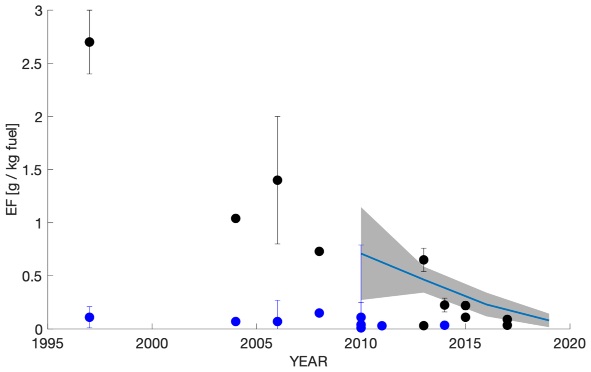
Figure 1 On-road measurements of emission factors from other studies. HDV (black) emission factors converge on LDV (blue) emission factors. Some studies do not give error bars. Gray patches and blue trend lines indicate findings from this study for the two highway sites (Redwood City, RWC, and San Rafael, SR) available during all time periods. The blue trend line shows the error-weighted mean of emission factors at these two sites during each time period. Gray patches indicate the estimated uncertainty in the error-weighted mean.

These prior observations show that typical heavy-duty, diesel-powered vehicles dominated on-road emissions of primary aerosol in the 1990s and early 2000s. However, in recent years, emission factors from typical heavy-duty vehicles have been dramatically reduced, such that PM_2.5 EFs of HDVs are now similar to those of light duty vehicles (LDVs) and have less than 0.05 g PM_2.5 kg⁻¹ of fuel burned. Control technologies, such as diesel particulate filters and selective catalytic reduction, are contributing to these reductions in EFs for HDVs.

While these improvements are seen in the typical HDVs, previous studies indicate that compliance of HDVs with emission technology requirements, and therefore HDV on-road emission factors, vary by up to an order of magnitude from location to location (Preble et al., 2018; Bishop, 2015; Haugen and Bishop, 2017, 2018). For example, Bishop (2015) and Haugen and Bishop (2017, 2018) found emission factors measured at the Port of Los Angeles were as much as an order of magnitude lower than those measured along a highway in Cottonwood, California, during the same season. While the gap between the two sites narrowed from 2013–2017, the mean emission factors measured in Cottonwood were still 3 times those measured at the Port of Los Angeles in 2017. Similarly, Preble (2018) found that, while 100 % of trucks at the Port of Oakland were registered by the state of California as being in compliance with HDV control technology regulations, compliance rates amongst HDVs at the Caldecott Tunnel (also in Oakland, CA) were below 90 %.

These studies highlight that variability in emission factors as a function of location may affect exposure. They point to the importance of characterizing the spatial variation in HDV emissions if we are to understand aggregate emissions from the sector and its localized impacts. To assess the potential for existing data sources to supply the needed information, here we explore the use of regulatory sensor networks (near-highway, hourly PM_2.5 and CO (or CO₂) measurements) paired with coincident traffic data, including LDV and HDV counts, to quantify the spatial variation in HDV EFs. Such data are widely available. For example, in the U.S., there are more than 550 regulatory sites at which PM_2.5 and CO are collocated, some of which have measurements spanning more than a decade (https://www.epa.gov/outdoor-air-quality-data, last access: 11 November 2020). Of these, 154 are located within 500 m of a highway. The large number of these sites and their longevity allow for examination of regional and temporal differences in EFs for HDVs across the United States. In the future, the approach we outline should be even more widely applicable when dense low-cost sensor networks, including aerosol and CO or CO₂, are available as a data source (e.g., Shusterman et al., 2016; Kim et al., 2018; Zimmerman et al., 2018). Because HDV emission control regulations vary regionally in the U.S., this method has the potential to shed light on regional differences in HDV EF trends.

We begin by describing a general method for using such data to derive the EFs of primary PM_2.5 from HDVs (Sect. 2). We then (Sect. 3) test our method by using data from four near-highway sites operated by the Bay Area Air Quality Management District (BAAQMD) in the San Francisco (SF) Bay area (Fig. 2a) over the period of 2009–2018. In Sect. 4, we discuss the relationship of these findings to measures of exposure.

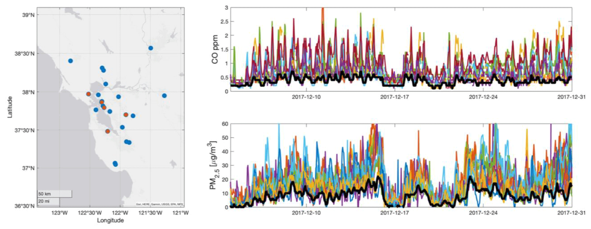
Figure 2 BAAQMD sites used in this study are shown in the left panel. Red dots show near-highway sites at which HDV emission factors were determined. Blue sites were used only for determining the regional signal. On the right-hand side, aerosol and CO at each BAAQMD site (various colors) are shown. The regional background (black), is defined as the lowest 10th percentile of all signals within a rolling 4 h window. Figure credit: Esri, HERE, Garmin, USGS, EPA, and NPS.

2 Data and methods

2.1 Aerosol and CO measurements

We use 1 h averaged observations from 18 of the BAAQMD regulatory sites which measure PM_2.5 using beta attenuation monitors and CO using the Thermo Fisher Scientific TE48i IR sensor. Some sites have been in operation since 2009, while others have been brought online as recently as 2018 or were operational for only a few years during this time period. Data were retrieved from https://aqs.epa.gov/aqsweb/documents/data_api.html (last access: 19 November 2021). Site locations are summarized, and example data are shown in Fig. 2. PM_2.5 and CO data from four near-highway sites (San Rafael, Redwood City, Berkeley Marina, and Pleasanton) are used to characterize EF_PM(HDV), and data from other sites are used to define regional signals.

2.2 Meteorology

Boundary layer height and wind speed and direction were retrieved from the European Centre for Meteorology and Weather Forecasting (ECMWF) ERA5 reanalysis (https://cds.climate.copernicus.eu/cdsapp#/dataset/reanalysis-era5-land?tab=form, last access: 12 October 2021). Typical diel cycles for boundary layer height and total wind speed are shown in Fig. S1.

We use this reanalysis to find wind speed, boundary layer height, and wind direction for each hour (2009–2020) at each of the BAAQMD sites. Wind data are then used for filtering PM_2.5 and CO measurements, as described below.

2.3 Traffic data

Total vehicle flow, fleet speed, and the percent of vehicles that are HDVs are taken from the Caltrans Performance Measurement System (PeMS) database (http://pems.dot.ca.gov, last access: 16 October 2021), which records these parameters at over 1800 locations on highways in the SF Bay area. We include all BAAQMD sites that are within 500 m of one major highway and use traffic count data from the PeMS measurement site closest to each air quality site. In cases of missing PeMS data, data were filled in with the median value associated with that parameter for a particular site in a particular year or, if not possible, retrieved from the second- or third-nearest sites. More details about the PeMS data, including a map of PeMS measurement sites, a list of sites used in this study, and example diels of truck flow and truck percent are presented in Figs. S2–S3 and Table S1.

2.4 The EMissions FACtor (EMFAC2017) model

In order to calculate EF_PM(HDV), as described in Sect. 2.5, we make use of the EMFAC2017 model to estimate both HDV and LDV emission factors for CO and a HDV and LDV fuel efficiency. We run this model for the four time periods of interest (2009–2011, 2012–2014, 2015–2017, and 2018–2020) by choosing the middle year for that period, specifying the location to be the nine counties under the BAAQMD's jurisdiction. We assign the vehicle class to either LDV or HDV by approximate vehicle length, as this is the manner in which PeMS classifies vehicles as being either LDVs or HDVs. These designations are summarized in the supplement of Fitzmaurice et al. (2022). We use EMFAC emission values across all speeds to obtain CO emission factor used to calculate EF_PM(HDV) for all sites during a given time period.

To estimate uncertainty in these emission factors at particular sites, we use the speed-dependent variance in EMFAC-derived emission factors. To do this, we first calculate speed-dependent CO emission factors (g CO kg⁻¹ fuel) and emission rates g CO₂ vkm⁻¹ for HDVs and LDVs for each time period as follows:

$$\begin{array}{}\text{(1)}& X_{\mathrm{speed},\mathrm{HDV}/\mathrm{LDV}}={\displaystyle \frac{{\sum }_{i=\mathrm{1}}^n{\mathrm{vkm}}_{i,\mathrm{speed}}{X}_{i,\mathrm{speed}}}{{\sum }_{i=\mathrm{1}}^n{\mathrm{vkm}}_{i,\mathrm{speed}}}}.\end{array}$$

Here, vkm is the EMFAC model's estimate of kilometers traveled per year by a particular vehicle class, and X is either the emission rate (g CO₂ vkm⁻¹) or emission factor in (g CO kg⁻¹ fuel). The EMFAC2017 model bins speeds (each 5 mph (8 km h⁻¹)), so we use spline interpolation to estimate the CO emission factor and emission rate hourly at each PeMS site corresponding to a BAAQMD site of interest. The 1σ variance of these estimates during times corresponding to those used to calculate EF_PM(HDV) are then used estimate uncertainty in emission rate and CO emission factors. These, in turn, are used to estimate uncertainty in EF_PM(HDV).

2.5 Derivation of EF_PM(HDV)

Our derivation of HDV EFs assumes that the relationship between the enhancement of PM_2.5 and CO, as observed near roads, can be scaled so that it represents particulate matter (PM) per unit of fuel burned by HDVs, as follows:

$$\begin{array}{}\text{(2)}& {\mathrm{EF}}_{\mathrm{PM}\left(\mathrm{HDV}\right)}=\mathit{\gamma }{\displaystyle \frac{{\mathrm{PM}}_{\mathrm{HDV}}}{{\mathrm{CO}}_{\mathrm{fleet}}}}{\displaystyle \frac{g{\mathrm{CO}}_{\mathrm{fleet}}}{\mathrm{kg}{\mathrm{fuel}}_{\mathrm{HDV}}}}.\end{array}$$

In this equation, γ=0.0008 and is the ideal gas law conversion factor, from (µg m⁻³ ppm⁻¹-CO) to ($g{\mathrm{PM}}_{\mathrm{2.5}}/g\mathrm{CO})$, where ppm is parts per million. A detailed derivation of Eq. (2) is described in Sect. S3. Below, we describe the steps used to calculate each term in Eq. (2).

The first term $\frac{{\mathrm{PM}}_{\mathrm{HDV}}}{{\mathrm{CO}}_{\mathrm{fleet}}}$ in the equation is derived from observations as the slope of a linear fit of near-road PM_2.5 (assumed to be primarily emitted by HDVs) and near-road CO (assumed to be emitted by both HDVs and LDVs). This term is derived by (1) isolating local enhancements of PM_2.5 and CO, (2) isolating roadway enhancements by using temporal and meteorological filters, and (3) fitting resulting roadway enhancements of PM_2.5 and CO to a line, as detailed below.

To isolate local enhancements from total signal PM_2.5 and CO, we first leverage the entire BAAQMD network to derive an hourly regional signal for each species. The regional signal is defined as the 10th percentile of the data across all 22 BAAQMD sites within a 5 h window of that hour (Fig. 2b). We choose the bottom 10th percentile rather than the absolute minimum in the hopes that the baseline captures regional mixing rather than just cleaner background air. In Sect. S4 in the Supplement, we show that, while the EF_PM(HDV) is slightly sensitive to the percentile and time window chosen, the sensitivity of EF_PM(HDV) to these parameters is smaller than estimated uncertainty in final EF_PM(HDV) values. This regional signal is assumed to be composed of background PM_2.5/CO transported to the region from elsewhere and region-wide sources of secondary aerosol/CO. We the find the enhancement by local primary emissions by subtracting the regional signal from total signal at each site.

We isolate primary emissions from on-road sources by considering only the morning commute times during fall and winter only and applying meteorological filters. These are times coinciding with relatively high traffic emissions and are too early in the day for the significant accumulation of new secondary aerosol. We find that the 06:00–08:00 LT (local time) period represents the optimal overlap of low boundary layer height (Fig. S1) and HDV emissions (Fig. S3). The combination of low boundary layer height and stable early morning conditions enhance the signal (Choi et al., 2012, 2014), allowing inferences about traffic from sites further away than would be possible during later morning or afternoon hours.

To avoid observations of stagnant air, we only include observations with wind speed above 0.5 m s⁻¹. Furthermore, for each site of interest, we exclude known fire events, and we filter out observations that occur when the BAAQMD site is upwind of the highway. An upwind event is defined as occurring when the wind direction deviates more than 90^∘ in either direction from the perpendicular line pointing from the highway nearest a BAAQMD site to that site. The result of these first two steps is enhancements in ΔPM_2.5 and ΔCO above the background.

The slope of a linear fit of all unfiltered ΔPM_2.5 and ΔCO (see Fig. 3) is defined as the enhancement ratio (units of µg m⁻³ ppm⁻¹ CO). Using the lengthy dataset, we can derive enhancement ratio for different percentages of HDVs in the vehicle fleet on the road. There are some high ΔPM_2.5 values uncorrelated with ΔCO, as shown in Fig. 3. In all cases, these points show little-to-no NO_x enhancement and thus are characteristic of a source that is not from HDVs. We make the assumption that LDV PM_2.5 EFs are negligible, and on-road primary emissions of aerosol are solely from HDV, implying that the enhancement ratio is equivalent to the term $\frac{{\mathrm{PM}}_{\mathrm{HDV}}}{{\mathrm{CO}}_{\mathrm{fleet}}}$. We discuss this assumption and the impact of correcting for LDV emissions further in Sect. 3.

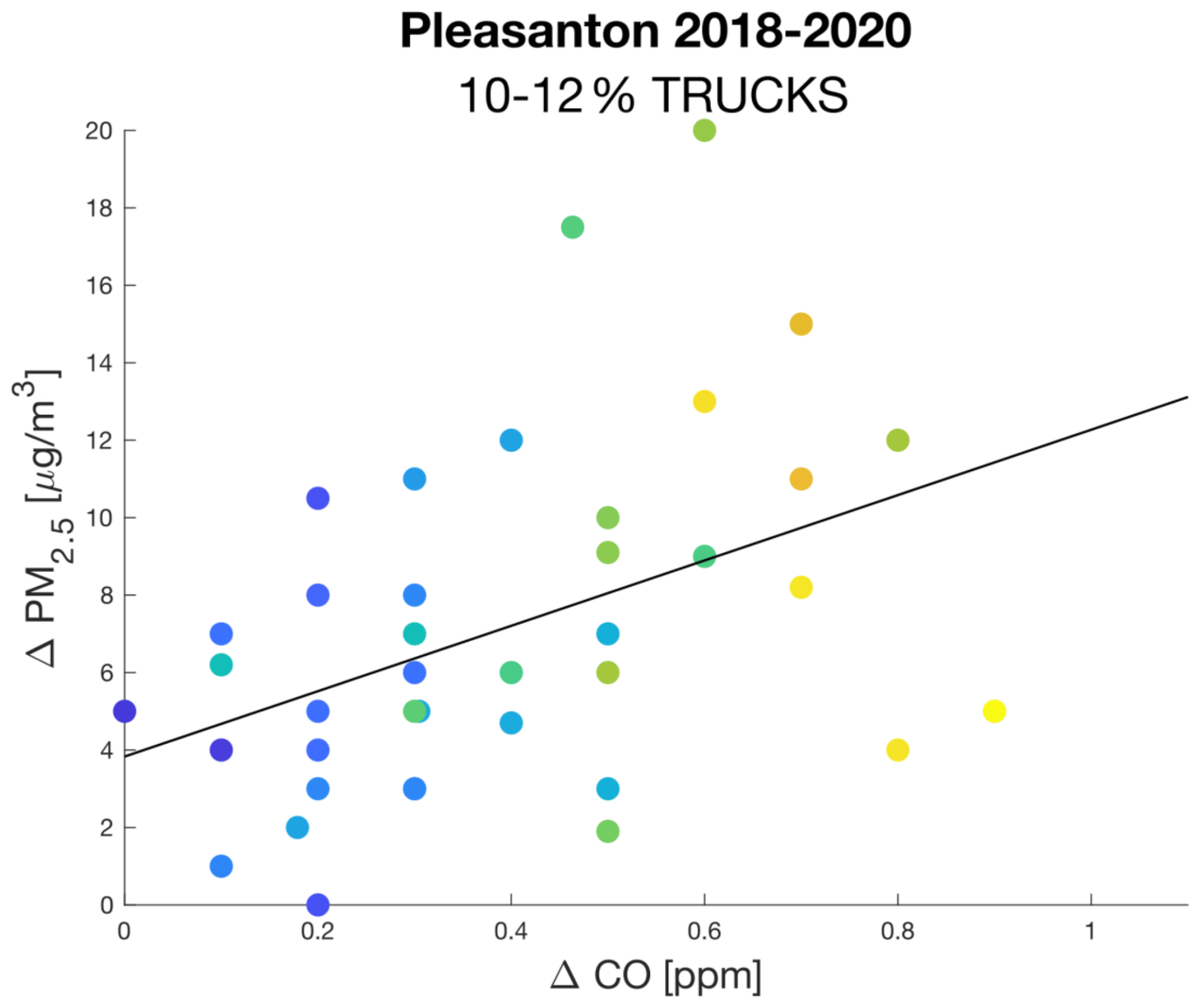
Figure 3 ΔPM vs. ΔCO at the Pleasanton site during the 2018–2020 time period, for which 10 %–12 % of traffic flow are trucks. Data are colored by NO_x concentration. These points are fit linearly to find the slope.

The term $\frac{g{\mathrm{CO}}_{\mathrm{fleet}}}{\mathrm{kg}{\mathrm{fuel}}_{\mathrm{HDV}}}$ can be calculated using the HDV fraction, t, and LDV and HDV CO emission factors (g CO kg⁻¹ fuel) and emission rates (g CO₂ km⁻¹) from EMFAC2017 model as follows:

$$\begin{array}{}\text{(3)}& {\displaystyle \frac{g{\mathrm{CO}}_{\mathrm{fleet}}}{\mathrm{kg}{\mathrm{fuel}}_{\mathrm{HDV}}}}={\displaystyle \frac{{\mathrm{EF}}_{\mathrm{CO}\left(\mathrm{HDV}\right)}t{E}_{\mathrm{HDV}}+{\mathrm{EF}}_{\mathrm{CO}\left(\mathrm{LDV}\right)}\left(\mathrm{1}-t\right)E_{\mathrm{LDV}}}{t{E}_{\mathrm{HDV}}}},\end{array}$$

where t is the HDV fraction, and E is emission rate.

Because, at a given site, we expect $\frac{{\mathrm{PM}}_{\mathrm{HDV}}}{{\mathrm{CO}}_{\mathrm{fleet}}}$ (but not EF_PM(HDV)) to vary linearly with the HDV fraction, we bin data by HDV fraction in increments of 0.02 and use the process above to calculate EF_PM(HDV) for each bin. Data and slopes for each bin are shown in Fig. S6. We then calculate EF_PM(HDV) for each site during a particular time period, using the average of the EF_PM(HDV) for each bin weighted by uncertainty. A detailed description of how we estimate the uncertainty in EF_PM(HDV) for each bin can be found in Sect. S6.

3 HDV emission factors from primary aerosols in the SF Bay area: 2009–2020

The result of this procedure is EF_PM(HDV) at four near-highway BAAQMD sties (Redwood City, Berkeley Marina, San Rafael, and Pleasanton) during the time periods of 2009–2011, 2012–2014, 2015–2017, and 2018–2020 (Fig. 4). We observe the EF_PM(HDV) decrease substantially over the decade (Figs. 1, 4), which amounts to a ∼ 9-fold reduction. We also observe substantial site-to-site differences in EF_PM(HDV). For example, during the 2018–2020 period, we see a range of a factor of ∼ 7 of 0.05 ± 0.06 g PM_2.5 kg⁻¹ fuel to a maximum of 0.35 ± 0.08 g PM_2.5 kg⁻¹ fuel. In addition, we observe different timing emission factor decreases between sites (e.g., Redwood City and San Rafael). For example, while emission factors at both Redwood City and Santa Rosa drop throughout the time period, values at San Rafael in the 2018–2020 time period are similar to those seen at Redwood City in 2012–2014, suggesting a difference in the timing of compliance to control technologies at each place. Both the temporal decrease and the site-to-site differences in EF_PM(HDV) are similar to prior reports derived using other approaches to data collection and interpretation (e.g., Haugen and Bishop, 2017, 2018).

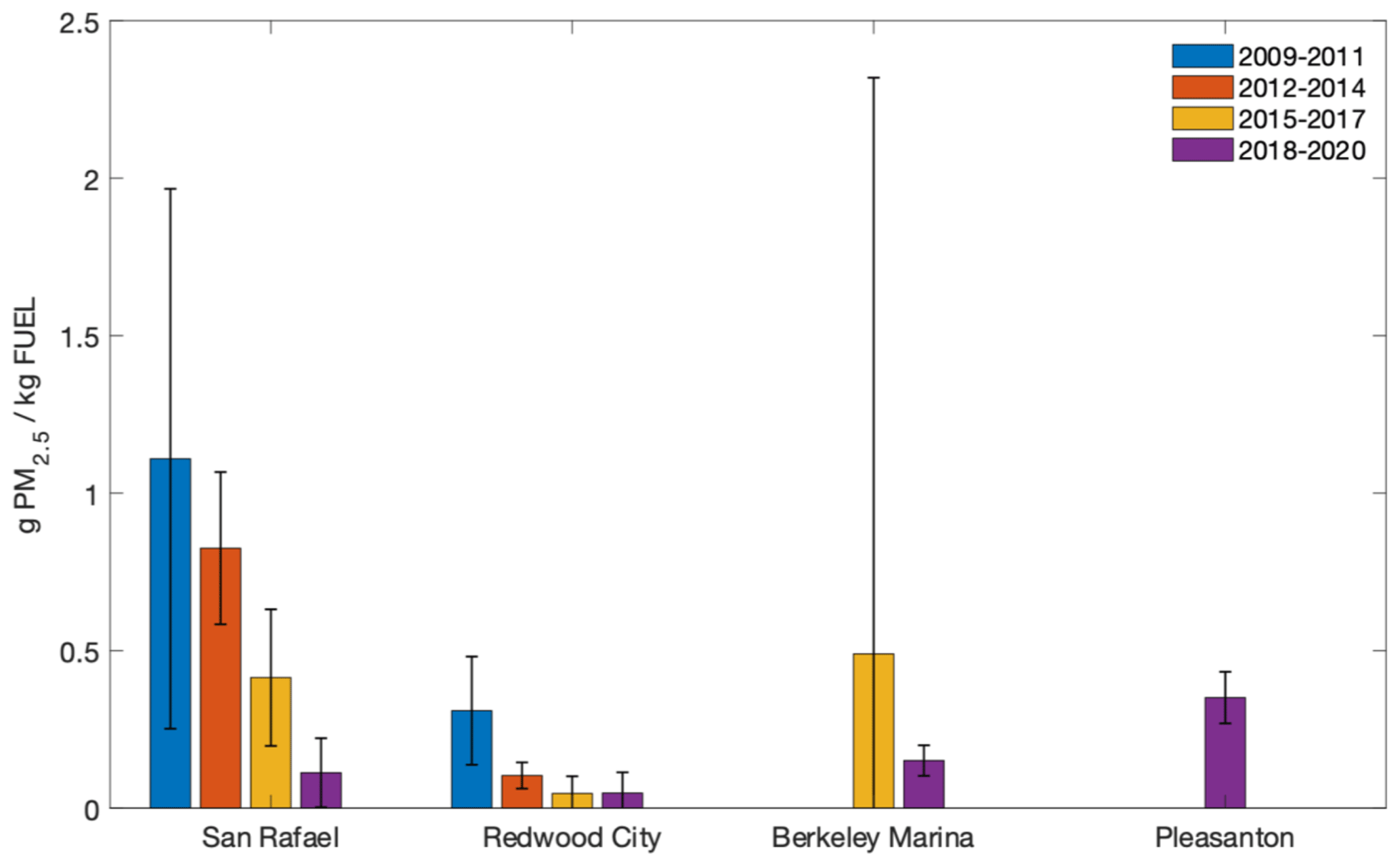
Figure 4 Fleet emission factors, derived from all sites, for all years, and binned by truck fraction are shown at the top. The HDV emission factor at near-highway sites during the 2009–2011, 2012–2014, 2015–2017, and 2018–2020 time periods.

In addition to being in line with observations from other studies, the observed decrease in EF_PM(HDV) follows progressively more stringent truck regulations by the state of California over that time. However, in the 2018–2020 period, observed EF_PM(HDV) are still higher than would be expected were all vehicles in compliance with Californian regulations. By 2020, California law required that all HDV models from the years 1995–2003 replace their engines with 2010 or newer models and that all HDV models from the year 1994 or newer use diesel particulate filters (DPFs; California Code of Regulations, 2022). Assuming that the fleet-wide average EF for models with 2010 or newer engines using DPFs is 0.03 g PM kg⁻¹ fuel, as observed by Haugen and Bishop (2018), we can use fuel usage by HDV model year in 2020 and emission factors for vehicles older than 1994 estimated by EMFAC2017 to estimate a fleet-wide average. Thus, a fleet-wide average should have an EF of 0.03–0.06 g PM kg⁻¹ fuel, if the trucks were fully compliant in 2018–2020. In contrast, we observe an average EF of 0.08 ± 0.03 g PM_2.5 kg⁻¹ fuel for 2018–2020. While our estimates overlap with the higher end of what is expected, counting uncertainty, it is larger than expected for a HDV fleet compliant with current regulations.

Non-exhaust vehicle emissions (e.g., tire wear and brake wear) may account for some of this discrepancy. However, we observe substantially higher emission factors at highways near the Pleasanton (0.35 ± 0.08 g PM kg⁻¹ fuel) and Berkeley Marina (0.15 ± 0.05 g PM_2.5 kg⁻¹ fuel) sites. Possible explanations for this discrepancy include exemptions from truck regulations, under which certain classes of HDVs traveling fewer than 15 000 miles (24 140.16 km) per year are eligible for exemptions, meaning that locally traveling HDVs may have higher emission factors than those traveling long distances (CARB, 2018b). The fact that HDVs registered in other states are not typically subject to Californian regulations, unless they enter specific areas, such as ports, and failure of or tampering with installed equipment is not taken into account.

In considering estimated EF_PM(HDV), it is important to consider two potential biases in our method, i.e., the impact of PM_2.5 emitted by LDVs and the potential for local sources to bias emissions estimates. As stated in Sect. 2, in calculating EF_PM(HDV), we assume that contribution of PM_2.5 from LDVs is negligible. This assumption is sound at the beginning of our period (2010s) of interest because reported values of EF_PM(HDV) were more than an order of magnitude higher than EF_PM(LDV) at that time (Fig. 1). More recently, as EF_PM(HDV) has decreased, this is less clear, especially without on-road estimates of EF_PM(LDV) and because LDVs also contribute non-tailpipe emissions of PM_2.5 from brake and tire wear. However, for 2020, EMFAC still estimates the ratio of EF_PM(HDV) : EF_PM(LDV) to be ∼ 8. Such a ratio would mean that even if only 5 % of vehicles were HDVs, then more than 60 % of PM_2.5 emissions are expected to be attributable to HDVs. This is an important concern, and we address it in two ways. First, we show that, even in the 2018–2020 period, the PM : CO enhancement ratio increases with the percent of HDVs regardless of total flow rate (Fig. 5a). We interpret the intercept of a linear fit with these data to be the PM_2.5 resulting from LDVs alone and note it to be much smaller than the impact of increasing HDVs by only a few percent. The observed PM_2.5 : CO intercept would correspond to an EF_PM(LDV) to be ∼ 0.01 g PM_2.5 kg⁻¹ fuel. This value is roughly consistent with tire and brake emission factors from EPA MOVES3 (EPA, 2020), although it is difficult to know the extent of braking at a given site, and estimates from previous studies of non-exhaust PM_2.5 by LDV vary widely (Fussell et al., 2022). Second, we explore the impact that LDV emissions might have on EF_PM(LDV). To understand the impact of LDV PM_2.5 emissions on our findings, we assume EF_PM(LDV) to be 0.01 g PM kg⁻¹ fuel and recalculate EF_PM(HDV). As shown in Fig. 5a, correction for LDV emissions in this way decreases estimated EF_PM(LDV), bringing the average value in the 2018–2020 period to 0.03, which is in line with what would be expected if all SF Bay area HDVs were in compliance with regulations during that period. However, even after this correction, EF_PM(HDV) at Pleasanton and Berkeley Marina are still substantially higher (0.32 ± 0.08 and 0.13 ± 0.05) than would be expected if all HDVs were compliant.

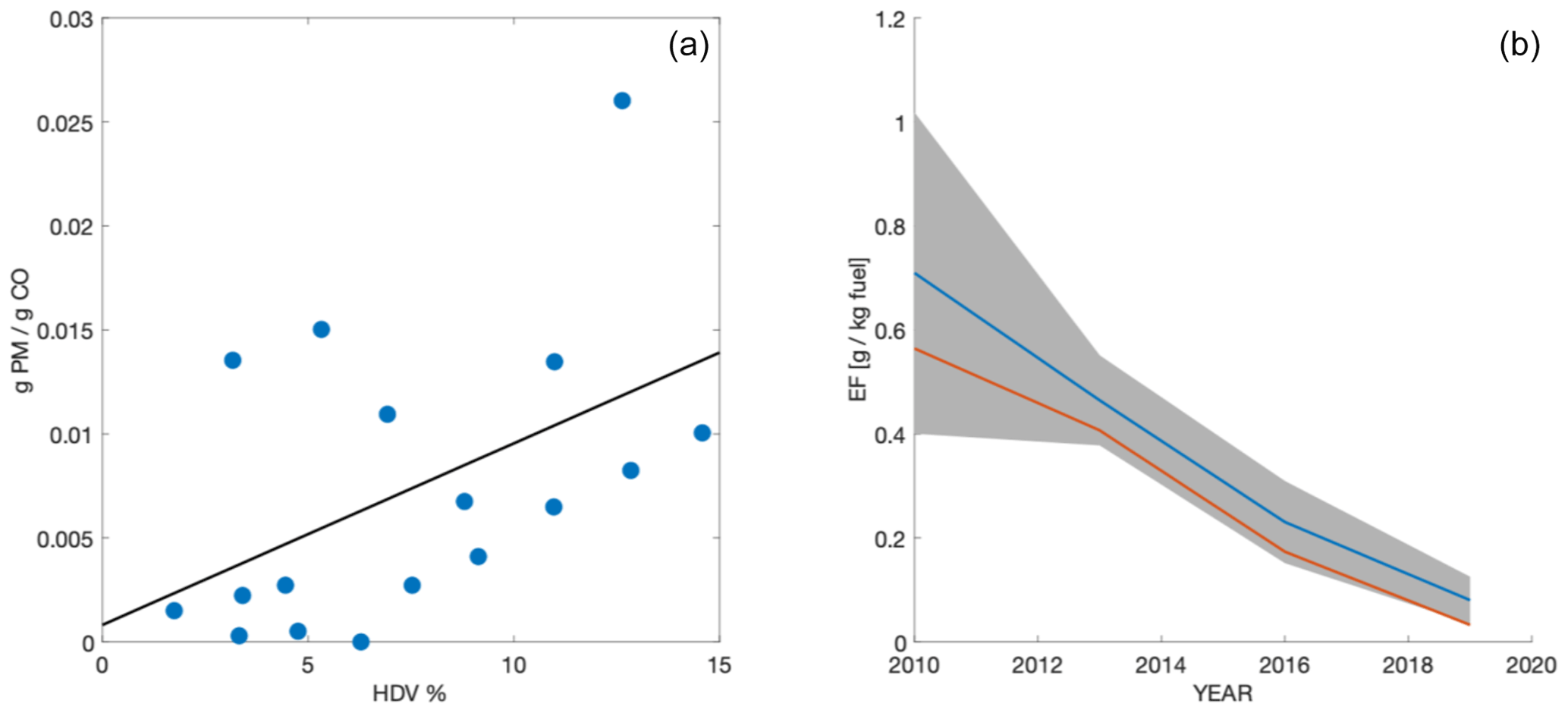
Figure 5 (a) Each point corresponds to the PM : CO enhancement ratio calculated via a linear fit between PM enhancement and CO enhancement at a particular near-highway site during the 2018–2020 time period for each bin of HDV (%). Laney College data are not included. The black line shows the linear fit corresponding to all points. (b) Trend in EF_PM(HDV) for RWC and SR (as shown in Fig. 1). The blue line indicates values calculated for the setting EF_PM(LDV)=0, while the orange line indicates values calculated using EF_PM(LDV)=0.002 g PM kg⁻¹ fuel. Gray patches indicate the estimated uncertainty in the error-weighted mean for the case where EF_PM(LDV)=0.

The second potential for bias in the method presented here is the influence of local, non-highway sources on measured PM_2.5 and CO enhancements. Because our method is dependent on finding the slope of PM_2.5 and CO, we expect this to eliminate contributions from non-combustion sources for which PM_2.5 and CO are uncorrelated. However, nearby combustion, such as non-highway vehicle sources, has the potential to influence EF_PM(HDV) results. For example, we consider the EF_HDV calculated for Laney College, a near-highway BAAQMD site not considered in the analysis above. The Laney College site instruments are located in a large parking lot. In the 2015–2017 and 2018–2020 period, we see significantly higher EF_HDV than observed at the four sites we deem to be reliably far from other sources. While it is possible that HDVs on the highway near Laney College are unusually high emitters, it is more likely that emissions from a nearby parking lot are responsible for the high inferred EFs. This is because PM_2.5 : CO emissions ratios are expected to be dramatically higher at low (parking lot) speeds compared to speeds typically seen on a highway, meaning that a comparatively small number of vehicles may contribute significantly to PM_2.5 : CO enhancement ratios (see Sect. S8 and Fig. S8). This example shows that, while the method developed in this paper has the potential to leverage existing data to highlight potential hotspots for EF_PM(HDV) non-compliance, care must be taken in interpretation of resulting emission factors.

4 Primary PM_2.5 exposure

To understand exposure from HDV PM_2.5, we calculate both a region-wide addition to aerosol burden by HDV emissions and an enhancement as a function of distance from a highway. Assuming a steady state, a box of 100 km in length, 160 m in height, and a wind speed of 1.2 m s⁻¹ (Fig. S6), and using fuel sales data (Moua, 2022) to estimate total HDV fuel used, we estimate a maximum region-wide enhancement of the order of 0.12 µg m⁻³ on a typical day in the 2018–2020 period, compared to an enhancement of 1.1 µg m⁻³ during the 2009–2011 period (Fig. S7). Decreases in emission factors over the past decade are countered by the increase in diesel fuel usage (70 %; Moua, 2022), such that there has been only a small change in typical regional exposure to primary PM from HDVs (see Fig. S1 for a diel cycle of the modeled region-wide enhancement). While an enhancement of 0.12 µg m⁻³ is small in comparison to average ambient PM_2.5 (8.3–14.4 µg m⁻³ for all BAAQMD sites in 2018), it is sizable in comparison to the average ambient BC (0.4–1 µg m⁻³ for all BAAQMD sites in 2018).

To gauge near-roadway exposure, PM_2.5 enhancement from HDVs was calculated as a function of distance from a highway, which was modeled by treating emissions from the highway as a Gaussian plume flowing perpendicular to a line source. Assuming that both the highway and point of measurement are at ground level, the simplified Gaussian plume dispersion for a line source yields the following:

$$\begin{array}{}\text{(4)}& \mathit{\lambda }{\mathrm{PM}}_{\mathrm{2.5}\mathrm{enh}}={\displaystyle \frac{\mathrm{2}}{\sqrt{\mathrm{2}\mathit{\pi }}u{\mathit{\sigma }}_z}},\end{array}$$

where λ is an emission rate per unit of highway length, u is the wind speed, and σ_z is a dispersion parameter. Using the average emission factor from the 2018–2020 time period, for a typical daytime HDV flow rate of 500 vehicles per hour (Fig. S2) and wind speed of 1.2 m s⁻¹ (Fig. S6), we calculate PM_2.5 enhancement as a function of perpendicular distance downwind of a highway. For unstable atmospheric conditions (${\mathit{\sigma }}_z=\frac{\mathrm{0.102}x}{{\left(\mathrm{1}+\frac{x}{\mathrm{927}}\right)}^{-\mathrm{1.92}}}$), enhancements drop to values of below 0.8 µg m⁻³ in the first 200 m. For stable conditions (${\mathit{\sigma }}_z=\frac{\mathrm{0.022}x}{{\left(\mathrm{1}+\frac{x}{\mathrm{1170}}\right)}^{\mathrm{0.7}}}$), such as those typical of early morning, enhancements of 1 µg m⁻³ are predicted up to a kilometer away.

5 Conclusions

We find that HDV EFs in the SF Bay area have decreased by about a factor of ∼ 9 over the last decade, consistent with trends reported in other analyses in this region and Los Angeles. We find that the spatial variation in HDV EFs remains large, indicating a wide range in the application of retrofit technologies and the possibility that vehicles legally exempt from compliance with the current standards are a significant portion of those on the road at the sampling sites. The method introduced in this paper has the potential to leverage existing regulatory (or other) data to examine long-term trends and highlight potential spatial heterogeneities in EF_PM(HDV).